Operational implementation of the ACCESS Numerical Weather Prediction systems · ·...

1

NMOC Operations Bulletin No. 83

Operational implementation of the ACCESS

Numerical Weather Prediction systems

21 September 2010

1. Introduction

On Tuesday 17 August 2010 the Bureau of Meteorology’s new operational “ACCESS” (Australian

Community Climate and Earth-System Simulator) Numerical Weather Prediction (NWP) systems

formally replaced the GASP, LAPS, TXLAPS and MESOLAPS NWP systems which were

switched off from that date. The ACCESS systems are based on the UK Met Office Unified

Model/Variational Assimilation (UM/VAR) system, and have been developed and tested by

research staff under the leadership of Dr Kamal Puri in the Earth System Modelling Programme of

the Centre for Australian Weather and Climate Research (CAWCR) and implemented

operationally by the Operational Development Subsection of National Meteorological &

Oceanographic Centre (NMOC).

This Bulletin provides an overview of the ACCESS NWP systems and output products and

expands on the preliminary ACCESS Operations Bulletin No. 80 of July 2009.

2. Background

For many years NMOC has run NWP models to provide a suite of analysis and prediction products

to support meteorological, oceanographic and climate services. Until recently these systems have

been developed in-house by the Bureau of Meteorology Research Centre (now the Centre for

Australian Weather and Climate Research, CAWCR). In 2005, in light of an increasing gap in the

performance of these local models compared with improving overseas model guidance, a decision

was made by the Bureau and CSIRO to jointly develop ACCESS, with the key aim to provide

world-class weather prediction and climate modelling capabilities to Australian users. Planning

for the development of ACCESS started in 2005 with the issue of two key documents, “Blueprint

for ACCESS” (Puri, June 2005) and “Project Plan for ACCESS” (Puri, September 2005).

The Blueprint provided an analysis of ACCESS stakeholder requirements and developed the scope

for ACCESS, based on these requirements and an analysis of Earth System Models in use at a

number of key international Centres. The Project Plan provided the scientific justification for

ACCESS and recommendations for the preferred options for the components together with an

estimate of the level of investment required for ACCESS to achieve its required objectives.

The development of ACCESS has followed the recommendations made in the Project Plan with

the key recommendation being to implement the Unified Modelling System(UMS) developed by

the United Kingdom Met Office (UKMO) which uses the Unified Model (UM) for atmospheric

prediction and variational (VAR) assimilation system.

Switching to UMS-based ACCESS systems has resulted in significant improvement in the

Bureau’s operational NWP forecast skill (see section 8 for verification results). The new system

2

also enables the incorporation of improvements developed by the UKMO, CAWCR and other

meteorological centres that have also adopted the UKMO model.

3. Key implementation dates

The ACCESS NWP components have been implemented via a progressive rollout schedule;

beginning on the Bureau’s previous NEC sx6 supercomputer and ending with implementation of

all systems on the new Oracle supercomputer “Solar”. Key implementation dates include:

• September 2009: Initial implementation of global, regional and tropical ACCESS domains

on the Bureau’s existing NEC supercomputer, running in parallel with the pre-existing

operational NWP models (GASP, LAPS, TXLAPS)

• 29 June 2010: Global, regional, tropical and Australian (mesoscale) ACCESS systems

declared operational on Solar and cessation of the NEC sx6 versions of these systems.

• 21 July 2010: Cessation of the ensemble-GASP system on the NEC sx6. Please note there

will be no replacement ACCESS-based ensemble system available for the time being.

• 17 August 2010: Final operational switchover to ACCESS-based systems. Cessation of

GASP, LAPS, TXLAPS, MESOLAPS, 5km MESOLAPS and TC-LAPS systems after the

afternoon 00UTC run, followed by decommissioning of the NEC sx6 supercomputer.

4. UM model description

Currently ACCESS uses version 6.4 of the Unified Model. Key features of various components

and physical parametrizations are outlined below.

4.1 Dynamics

Prognostic variables: u, v, w (zonal, meridional, vertical winds), density (specifically, the mass of

dry air per unit volume of moist air), potential temperature, and mixing-ratios of water-vapour,

cloud-liquid-water, and cloud-frozen-water, all with respect to dry-air. Equation set is non-

hydrostatic.

Grid: Arakawa-C grid in the horizontal, Charney-Phillips (thermodynamic and moisture variables

stored on half-levels) in the vertical. (Further details of the horizontal and vertical grid structure of

the ACCESS model are discussed in the appendix to this Bulletin.)

Advection: two-time-level semi-Lagrangian, with non-interpolating scheme for vertical advection

of temperature. Exception is density, which is treated in Eulerian fashion.

Acoustic terms: treated using a semi-implicit approach, yielding a Helmholtz equation for the

Exner pressure tendency, which is solved using a preconditioned generalised conjugate residual

method.

4.2 Cloud

Smith (1990) diagnostic cloud scheme based on conserved variables TL and qT (liquid/frozen

water temperature and total water content respectively) and a sub-grid scale probability distribution

of these variables, from which the cloud amounts and water contents are derived using an assumed

critical relative humidity. The scheme is modified such that only water clouds are defined from TL

and qT and a sub-grid probability distribution. Ice water content is determined by the prognostic

mixed phase microphysics scheme with ice cloud fraction calculated diagnostically from ice water

content. An additional parametrization to derive cloud area is included, where the approach is to

interpolate TL and qT to higher effective vertical resolution and use the cloud scheme on these

interpolated levels. The cloud on these sublayers is assumed to be maximally overlapped so that

the area cloud fraction that is seen by the radiation scheme is given by the maximum of the

sublayer values of the volume cloud fraction.

3

4.3 Radiation

Modified version of Edwards and Slingo (1996) scheme based on rigorous solution of the two-

stream scattering equations including partial cloud cover. Full treatment of scattering and aerosols.

Consistent treatment of cloud radiative properties in solar and thermal regions of spectrum. Ice

crystals are treated as non-spherical.

4.4 Boundary-Layer

Mixing in unstable layers uses the first order non-local scheme of Lock et al. (2000) that

parameterises eddy diffusivity profiles of unstable (well-mixed) layers driven either by fluxes at

the surface or by cloud-top processes.

Boundary layers are classified according to 7 separate types with unstable layers identified using a

parcel ascent/descent method. Cumulus mixing uses the mass-flux convection scheme.

Entrainment rates across the inversion at the top of the boundary layer are specified using an eddy

diffusivity scheme of Lock (1998; 2001) scaled using cloud-top cooling rates.

Mixing in stable boundary layers uses the local Richardson number first order closure of Louis

(1979) with stability dependent surface exchanges calculated using Monin-Obukhov Similarity.

4.5 Precipitation

Wilson and Ballard (1999) single-moment bulk microphysics scheme with explicit calculation of

transfers between vapour, liquid and ice phases. The one ice water prognostic variable is split by a

diagnostic relationship into ice crystals and aggregates, which are treated separately in the

microphysical transfer terms before being recombined after the calculations. The microphysical

processes calculated in the scheme are: sedimentation of ice and rain, heterogeneous and

homogeneous nucleation of ice particles, deposition and sublimation of ice, aggregation, riming

and melting of ice, collection of cloud droplets by raindrops, autoconversion and accretion

production of raindrops, and evaporation of rain (condensation and evaporation of cloud water is

performed by the cloud scheme).

4.6 Convection

Modified mass-flux scheme based on Gregory and Rowntree (1990).

Cumulus convection is diagnosed if air at the first model level is unstable to adiabatic ascent above

the lifting condensation level.

The cloud-base mass-flux is calculated based on the reduction to zero of convectively available

potential energy (CAPE) over a given timescale. A number of CAPE closure schemes are

available, and we use different options depending on the resolution of the particular NWP model.

The treatment of entrainment and detrainment for shallow convection is based on the similarity

theory developed by Grant and Brown (1999). For deep convection, entrainment is using

prescribed profiles, and detrainment is using an adaptive detrainment scheme.

The representation of convective momentum transport (CMT) for deep and shallow convection is

based on an eddy viscosity model.

4

4.7 Land Surface interaction

Met. Office Surface Exchange Scheme (MOSES) II: Additionally includes "tile" scheme with

separate surface-atmosphere fluxes calculated for each surface type present in a given gridbox.

4.8 Gravity-Wave Drag

Flow blocking scheme that simplifies diagnosis of hydrostatic gravity waves and low level drag

based on Froude Number.

5. Observational data assimilation

The ACCESS system uses a four-dimensional variational data assimilation scheme (4DVAR).

This scheme results in a much improved use of observations compared to the scheme used by the

GASP and LAPS systems, firstly by using more data and also by making better use of all data.

4DVAR systems take into account time differences between various observations, and also the

time differences between the observations and the nominal analysis time in a dynamically

consistent way. 4DVAR also allows for multiple reports from the same station to be used, in effect

assimilating tendency information as well the full observations. Finally, the variational approach

performs a dynamical initialization during the analysis – so that the initialization does not disrupt

the fit of the analysis to the observations.

Observations currently used by ACCESS include:

• Land surface stations, ships and drifting buoys: surface pressure, 2m temperature, 10m

winds and 2m relative humidity.

• Radiosondes: temperature, wind and relative humidity

• Pilot and profiler winds

• ATOVS radiances (HIRS, AMSU-A and AMSU-B)

• AIRS radiances (62 channels)

• Geostationary AMV winds including locally calculated 6 hourly cloud drift winds from

MTSAT-2

• Scatterometer winds (ASCAT)

• Aircraft (AMDAR) winds and temperatures

ACCESS does not currently assimilate the manually derived synthetic mean sea level pressure

“PAOB” data (Seaman and Hart 2003) previously used in GASP and LAPS. As a result, NMOC

ceased production and distribution of PAOBs as of 17 August 2010.

Observational data is subjected to various quality control checks including:

• Background checks – all observations are required to be within specified tolerances of the

background. The tolerances are a function of both observation and background error

variances. The background error variances are flow dependent – using a regression against

smoothed fields.

• Buddy checks between some observations:

o surface-surface,

o aircraft – aircraft,

o AMV – AMV,

o radiosonde – radiosonde and

o radiosonde – aircraft

5

• Satellite sounders (ATOVS and AIRS) subjected to:

o 1dVAR quality control checks

o Scan-dependent bias correction

o Fixed version of Harris and Kelly (2001) with 850-300 hPa thickness and 200-50

hPa thickness as the airmass bias predictors.

o Window channel checks

• AMSU-B data is also subjected to cirrus and scattering index checks

• All observations thinned in space and time.

• All observations are assigned a Probability of Gross Error (PGE) which is adjusted during

the variational minimization. Observations where PGE > 0.5 are given zero weight.

Data assimilation for most ACCESS systems (excepting the 5km ACCESS-C forecast-only

models) is performed every 6 hours (for basetimes at 00,06,12,18 UTC) using a centred 6 hour

observational data window. Due to forecast timeliness considerations, the ACCESS-R and

ACCESS-A systems commence their main data assimilation and forecast steps within 2 hours

of the nominal basetime for the model run (refer to table 2 in section 7 for timing details) and

before the end of the 6 hour data assimilation window. In order to assimilate all observational

data received for the full 6 hour window (and therefore improve the analysis accuracy), a

second “update” assimilation step is run 4 hours later. A short 6-hour forecast starting from

this update analysis provides the first guess for the next assimilation step. Compared with the

main run the update run assimilates considerably more satellite observations (e.g. AIRS,

ATOVS and QUIKSCAT) and aircraft observations (AMDAR and AIREP). Model timings

and nesting strategies are discussed further in section 7.

6. Main differences

From a user’s perspective, the main differences between the old numerical weather prediction

systems and the ACCESS systems include:

• Use of a hybrid vertical level structure in ACCESS rather than sigma levels. This will

affect any users of raw model data and is discussed further in Section 9 and the appendix.

• The horizontal and vertical staggering of fields on the native model grids, as discussed in

Section 4 and the appendix.

• The initial ACCESS model domains and spatial resolution are generally very similar to the

previous GASP/LAPS systems. The only significant changes to domains has been the

rationalization of the previous 0.125° MESO_LAPS and the 0.10° MA_LAPS mesoscale-

assimilation models to a single 0.11° ACCESS-A Australian mesoscale assimilation &

forecast system. See section 7 for a brief outline of system domains and resolutions.

• Evaporation and precipitation related fields are continuously accumulated throughout the

model run from the start of the assimilation window (currently set to 3 hours before the

analysis base-time). Hence fields such as accumulated precipitation will most likely be

non-zero at the analysis output step. NOTE: Most output fields are instantaneous ("snap-

shots" in time). For any time-averaged fields (e.g. average mean sea level pressure,

radiation fields, surface heat fluxes etc), as well as maximum and minimum screen

temperatures, the time period is the difference between the previous output time and the

field's validity time.

• Vertical velocity (m/s) replaces omega (Pa/s) as the parameter representing vertical motion

in the atmosphere although an approximately derived omega will be provided in the short-

term for users reliant on omega.

• Soil levels in ACCESS are at 0.1, 0.25, 0.65 and 2.0 m (whereas the previous LAPS levels

were at 0.035, 0.175, 0.64 and 1.945 m)

• New fields, including screen-level horizontal visibility, fog fraction and 10m wind gusts,

are available in the model outputs.

6

7. Operational ACCESS system configurations

It is envisaged that upgrades to ACCESS will be tested via semi-regular parallel test suites before

implementation. The initial ACCESS rollout has been designated as “Australian Parallel Suite 0”

(APS0) with domains and resolutions chosen to be similar to the existing operational NWP system

domains, as shown in Table 1 and Figure 1. Future model upgrades will be designated as APS1,

APS2 etc.

Figure 1: Domains of initial APS0 ACCESS models

NWP system Domain Type Resolution Domain limits S-N,W-E (lat x lon) Duration

(hours)

Runs

(UTC)

ACCESS-G Global Assim + Forc N144 (~80km) -90.00S to 90.00N, 0.00E to 358.75E (217x288) +240 00, 12

ACCESS-R Regional Assim + Forc 0.375° (~37.5 km) -65.00S to 17.125N, 65.00E to 184.625E (220x320) +72 00, 12

ACCESS-T Tropical Assim + Forc 0.375° (~37.5 km) -45.00S to 55.875N, 60.00E to 217.125E (270x420) +72 00, 12

ACCESS-A Australia Assim + Forc 0.11° (~12 km) -55.00S to 4.73N, 95.00E to 169.69E (544x680) +48 00, 06,

12, 18

Brisbane Forc 0.05° (~5 km) -31.00S to -22.05S, 148.00E to 155.95E (180x160)

Perth Forc 0.05° (~5 km) -37.00S to -28.05S, 112.00E to 119.95E (180x160)

Adelaide Forc 0.05° (~5 km) -39.50S to -30.55S, 132.00E to 141.95E (180x200)

VICTAS Forc 0.05° (~5 km) -46.00S to -34.05S, 139.00E to 150.95E (240x240)

ACCESS-C

Sydney Forc 0.05° (~5 km) -38.00S to -30.05S, 147.00E to 154.95E (160x160)

+36 00, 12

ACCESS-TC Tropical

Cyclone Assim + Forc 0.11° (~12 km) Relocatable within the ACCESS-T domain: 30°x30° +72 00, 12

Table 1: ACCESS APS0 model domains & resolutions. (NOTE: The ACCESS-TC system is

currently undergoing development prior to testing and implementation, expected before the

start of the 2010/2011 cyclone season.)

For APS0, data assimilation occurs 4 times daily for nominal assimilation basetimes of 00, 06, 12

and 18 UTC. However, for ACCESS-G, T, TC and C, full model forecasts are only run from the

00 and 12 UTC analyses. In contrast, for ACCESS-R & A full model forecasts are run 4 times

daily from the 00, 06, 12, 18 UTC analyses. For ACCESS-R & A, a second “update” data

assimilation step is run 4 hours later than the “main” run to make use of any additional

7

observational data that were not available at the time of the earlier “main” assimilation step.

Typical model runtimes and output data availability times are listed in Table 2. (Note that the

ACCESS-R, A & C systems are run at times to fit into the local forecast schedule which varies

with the advent of daylight savings time between early October to early April each year.)

NWP system Run (UTC) Boundary condition source Assimilation

start time (UTC)

Analysis/Forecast

product availability

time (UTC)

ACCESS-G

00 assim + forc

06 assim

12 assim + forc

18 assim

n.a. (not applicable)

n.a.

n.a.

n.a.

04:55

11:25

16:55

23:25

05:30 / 05:50

12:30 / n.a.

17:30 / 17:50

00:30 / n.a.

ACCESS-R

00 assim + forc

00 assim update

06 assim + forc

06 assim update

12 assim + forc

12 assim update

18 assim + forc

18 assim update

ACCESS-G (12UTC)

ACCESS-G (00UTC)

ACCESS-G (00UTC)

ACCESS-G (00UTC)

ACCESS-G (00UTC)

ACCESS-G (12UTC)

ACCESS-G (12UTC)

ACCESS-G (12UTC)

01:55*

05:55*

07:55*

11:55*

13:55*

17:55*

19:55*

23:55*

02:15* / 02:40*

08:15* / 08:40*

14:15* / 14:40*

20:15* / 20:40*

ACCESS-T

00 assim + forc

06 assim

12 assim + forc

18 assim

ACCESS-G (12UTC)

ACCESS-G (00UTC)

ACCESS-G (00UTC)

ACCESS-G (12UTC)

03:30

10:55

12:30

22:55

03:55 / 04:10

10:20 / n.a.

15:55 / 16:10

23:20 / n.a.

ACCESS-A

00 assim + forc

00 assim update

06 assim + forc

06 assim update

12 assim + forc

12 assim update

18 assim + forc

18 assim update

ACCESS-R (00UTC main)

ACCESS-R (00UTC update)







~02:25*

~06:15*

~08: 25*

~12:15*

~14: 25*

~18:15*

~20: 25*

~00:15*

03:05* / 04:10*

09:05* / 10:10*

15:05* / 16:10*

21:05* / 22:10*

ACCESS-VT 00 forc

12 forc



n.a.

n.a.

n.a. / 03:10*

n.a. / 15:10*

ACCESS-SY 00 forc

12 forc



n.a.

n.a.

n.a. / 03:00*

n.a. / 15:00*

ACCESS-BN 00 forc

12 forc



n.a.

n.a.

n.a. / 03:00*

n.a. / 15:00*

ACCESS-AD 00 forc

12 forc



n.a.

n.a.

n.a. / 03:00*

n.a. / 15:00*

ACCESS-PH 00 forc

12 forc



n.a.

n.a.

n.a. / 03:00*

n.a. / 15:00*

Table 2: Typical assimilation commencement (i.e. observational data cutoff) times and

output product availability times for APS0 ACCESS models. Any times marked with an

asterisk will be 1 hour earlier during the Australian summertime daylight savings period

(October to April)

8

8. Forecast performance

Detailed testing of the global (ACCESS-G; N144L50) and Australian region systems (ACCESS-R;

37.5kmL50) including 4DVAR has been ongoing since July 2008, and more recently ACCESS-A

(~12kmL50), ACCESS-T (37.5kmL50) and ACCESS-C (5kmL50) initially by CAWCR and then

NMOC. The suite of ACCESS systems is robust and continues to perform well and forecasts show

large improvements in skill relative to the Bureau’s previous operational global and regional

systems (GASP and LAPS).

8.1 Subjective evaluations of ACCESS-G, ACCESS-R and ACCESS-C

After an extensive period of assessment it has been found that ACCESS-G MSLP forecasts are

continuing to produce useful guidance to at least 144 hours and are a clear improvement on the

previous operational system (GASP). Often these forecasts are comparable with EC model output

in their ability to capture the “big picture” broad scale circulation in the medium range. However,

limitations in horizontal spatial resolution of ACCESS-G (~80km) compared to the UKMO

(~25km) and ECMWF (~16km) models are evident in cyclogenetic situations. For example,

ACCESS-G underestimates the forecast depth of cut off lows in the Tasman Sea, leading to a

negative bias in the associated gradient winds. Of particular note is the apparent deficiency in the

forecast evolution of the upper flow over the SE Indian Ocean as a result of underestimation of the

amplitude and intensity of upper troughs as they approach the WA region. This can lead to poor

forecasts of cyclogenesis to the south of WA, on occasions as early as +72 hours. Moreover, due

to the lack of sharpness of upper troughs potential cutting-off processes may be missed, leading to

forecast full latitude troughs progressing too fast across Australian longitudes. ECMWF and

UKMO models can display this deficiency also but they tend to recognise the cutting-off process

24 hours earlier in the forecast sequence than ACCESS-G. In addition, this occasional lack of

appropriate definition of upper features over WA early in the forecast sequence may lead to

amplitude errors of frontal systems in the longer term over SE Australia.

Rainfall forecasts in the longer term appear to be useful (forecast statistics are discussed in detail in

section 8.3). However it is noted that ACCESS-G tends to have excessive rainfall rates at +48/+72

hours in NW cloud bands.

ACCESS-R is performing well and is superior to the LAPS MSLP forecasts particularly at 48 and

72 hours. However, in westerly regimes errors propagating from the western boundary start to

become evident in Australian longitudes at +72 hours. Hence, in westerly regimes, the MSLP

guidance from ACCESS-G at +72 hours is likely to be more reliable than ACCESS-R in spite of

the differences in spatial resolution. Conversely, in cut-off low situations once the cutting-off

process has been captured, ACCESS-R is likely to produce deeper systems with more realistic

peripheral wind speeds than ACCESS-G.

Figure 2 illustrates the good guidance provided by an ACCESS-R 48-72 hour rainfall forecast for

14 July 2010, although maximum rainfall rate in SE NSW, shown in the analysis, was

underestimated. The forecast rainfall areas appear to be more sharply defined than in the analysis

leading to an underestimation of the number of grid points raining.

9

Figure 2: ACCESS-R 48-72 hour rainfall forecast with verifying analysis for 9am 14 July

ACCESS-C low level vector wind field analyses and forecasts appear to be realistic and provide

good guidance to 36 hours on the timing of changes over SE Australia. MSLP patterns appear to be

noisy in the regions of enhanced orography in enhanced westerly flow over SE Australia and over

Tasmania. These detailed MSLP patterns are not necessarily spurious. For a discussion of the

influence of enhanced orography on forecast MSLP patterns and rainfall see Mass et al 2002.

Excessive forecast rainfall rates have been noted particularly over SE Qld and eastern NSW in

areas of high topography. Recent model tuning in CAWCR has led to improved rainfall forecasts

in these regions. An example of an outstanding 24 hour forecast in the Vic-Tas region for 00 UTC

for 4 August 2010 is illustrated in Figure 3. Note the very good timing of the front across Victoria

and the location of the low SW of Tasmania and the peripheral wind field.

Figure 3: ACCESS-C (VicTas) 24 hour 10m vector wind field forecast for 00 UTC 4 August 2010

and verifying analysis.

10

The ACCESS-C (Vic-Tas) 24 hour rainfall forecast for 9 am 2 August 2010 is illustrated in figure

4. Maximum rainfall totals in this case were slightly underestimated in the Alps but the overall

coverage was very good.

Figure 4: ACCESS-C (VicTas) 24 hour rainfall forecast for 9am 2 August 2010 and verifying

observational analysis.

A comment on the recent performance of ACCESS-C for the weather event of 14/15 August 2010

over SE Australia from the Victoria Regional Office (VRO) of the Bureau stated that “the VRO

forecasters made very good use of the ACCESS fields during the wind and rain event a couple of

days ago. The diagnostics were very accurate for the short term overnight predictions. Staffing

and forecasting decisions were based on this information and everything went very well. So it

doesn’t just look good, it IS good – particularly in the short term.”

8.2 Verification of model forecasts versus own analysis

ACCESS-G global system

Figure 6 shows the anomaly correlation scores for the period 1 January to 31 March 2010 from

ACCESS-G (N144L50, which represents a horizontal resolution of ~80km), and other global

models. The differences in performance between ACCESS-G and the UKMO system can be

attributed to a number of factors; namely

(i) resolution differences: ACCESS-G is N144 while UKMO is N512 (~25 km),

(ii) differences in the amount of data used in the two systems; ACCESS-G does not

currently assimilate IASI and GPS-radio occultation data, and

(iii) UKMO changes to assimilate cloudy radiances have not yet been implemented in

ACCESS.

A long term time series of S1 Skill Scores for the various global models are shown in figure 6.

The dramatic improvement of ACCESS-G compared to GASP is very evident – this is expected to

improve even further when we upgrade to the high resolution APS1 system in 2011.

11

Figure 5: Anomaly correlations for global model mean sea level pressure forecasts for the

Australian region for the period 01 April 2010 to 30 June2010 for ACCESS-G, GASP,

European Centre ECSP, United States USAVM, UK Met Office UKGC and Japanese Met

Agency JMAGSM. Higher correlations indicate a better performance. The level of useful

skill has been empirically determined to be 60%. The useful skill of ACCESS G now extends

to around 6 days and ACCESS G is better performed than the former Bureau global model

GASP.

Figure 6: Comparison of ACCESS-G (green cross) Mean Sea Level pressure 48 hour

forecasts (S1 skill score) with GASP (green), US (light blue), JMA (blue), UK (magenta) and

ECMWF (red). There has been a significant improvement in the ACCESS-G skill score

(represented by the green cross which is a eight month mean only) compared to the previous

operational global model (GASP)

12

ACCESS-R regional system

ACCESS-R is performing well to 48 hours. However, model performance at 72 hours, while better

than LAPS, is generally not as skilful as the equivalent ACCESS-G forecast in a westerly regime.

Figures 7 and 8 show performance statistics from ACCESS-R and LAPS for the period 31 August

2009 to 13 August 2010. The improvements with ACCESS-R (lower S1 Skill Score, lower RMS

errors and smaller bias magnitudes) are quite dramatic. However, it can be seen in figure 8 that,

while ACCESS verifies considerably better in the low to mid levels, above 200 hPa it does tend to

display somewhat larger biases in the geopotential height and temperature fields. This is thought to

be related to the fact that GASP and LAPS required fairly heavy Newtonian-damping applied to

their upper levels to keep them stable whereas such damping has not been used at all in the current

ACCESS systems. Improved treatment of the upper levels has been flagged as an area for research

in the next APS1 model version – it is expected that assimilation of GPS-radio occultation data

will improve the high upper-level performance significantly.

a)

b)

c)

Figure 7: Verification of Regional model Mean Sea Level pressure forecasts for the

Australian Region averaged over the period 31 August 2009 to 13 August 2010 for LAPS

(red) and ACCESS-R (green) for a) S1 skill Score, b) RMS error, c) bias. All fields are self-

verified, i.e. the forecasts from each system are compared to the system's own analysis.

Calculations have been performed on the model grid, from 45°S to 10°S, and 110°E to 155°E.

The vertical scale is in units of 0.1 hPa

13

a)

b)

c)

Figure 8: Verification of Regional model upper level forecasts for the Australian Region

averaged over the period 31 August 2009 to 13 August 2010 for LAPS (red) and ACCESS-R

(green) for a) geopotential height (units=0.1 m), b) temperature (units=0.1 °C), c) wind speed

(units=0.1 m/sec), at forecast range +48 hours. RMS error is shown on left, bias on right. All

fields are self-verified, i.e. the forecasts from each system are compared to the system's own

analysis. Calculations have been performed on the model grid, from 45°S to 10°S, and 110°E

to 155°E.

14

ACCESS-T tropical system

ACCESS-T, which replaces TXLAPS, appears to be performing well, capturing and maintaining

relatively weak low-level tropical circulations. It has been noted however, that tropical cyclones in

the NW Pacific have not been well represented. One particular case of typhoon “Conson” which

passed across the northern Philippines in July 2010 with a significant impact, as a category 1 storm

with maximum sustained wind speeds of 80 kts, was barely represented as a weak tropical

circulation with a minimal MSLP signature. The synthetic vortex “bogussing” of tropical cyclones

circulations which has previously been used in TXLAPS analyses is currently under development

in CAWCR for inclusion in the ACCESS assimilation systems and should provide enhanced

guidance in the Australian tropical cyclone season of 2010/2011.

Figures 9 and 10 show a similar improvement in ACCESS-T over TXLAPS over the extended

tropics during the period 15 September 2009 to 13 August 2010.

a)

b)

c)

Figure 9: Verification of tropical model Mean Sea Level pressure forecasts (S1 skill score) for

the tropical region averaged over the period 15 September 2009 to 6 August 2010 for

TXLAPS (red) and ACCESS-T (green) for a) S1 skill Score, b) RMS error, c) bias. All fields

are self-verified, i.e. the forecasts from each system are compared to the system's own

analysis. Calculations have been performed on the model grid, from 40°S to 22°N, and 100°E

to 170°E. The vertical scale is in units of 0.1 hPa

15

a)

b)

c)

Figure 10: Verification of tropical model upper level forecasts for the tropical region

averaged over the period 15 September 2009 to 6 August 2010 at forecast range +48 hours

for TXLAPS (red) and ACCESS-T (green) for a) geopotential height (units=0.1 m), b)

temperature (units=0.1 °C), c) wind speed (units=0.1 m/sec). RMS error is shown on left,

bias on right All fields are self-verified, i.e. the forecasts from each system are compared to

the system's own analysis. Calculations have been performed on the model grid, from 40°S to

22°N, and 100°E to 170°E.

16

ACCESS-A Australian mesoscale system

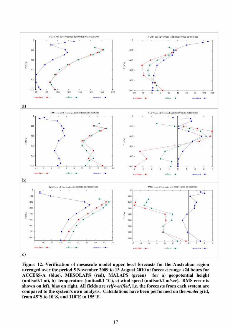
Figures 11 and 12 show a similar improvement in ACCESS-A over both MESOLAPS_PT125 and

MALAPS_PT100 over the Australian mesoscale domain during the period 15 September 2009 to

13 August 2010.

a)

b)

c)

Figure 11: Verification of mesoscale model Mean Sea Level pressure forecasts for the

Australian region averaged over the period 5 November 2009 to 13 August 2010 for

ACCESS-A (blue), MESOLAPS (red), MALAPS (green) for a) S1 skill Score, b) RMS error,

c) bias. All fields are self-verified, i.e. the forecasts from each system are compared to the

system's own analysis. Calculations have been performed on the model grid, from 45°S to

10°S, and 110°E to 155°E. Vertical scale is in units of 0.1 hPa

17

a)

b)

c)

Figure 12: Verification of mesoscale model upper level forecasts for the Australian region

averaged over the period 5 November 2009 to 13 August 2010 at forecast range +24 hours for

ACCESS-A (blue), MESOLAPS (red), MALAPS (green) for a) geopotential height

(units=0.1 m), b) temperature (units=0.1 °C), c) wind speed (units=0.1 m/sec). RMS error is

shown on left, bias on right. All fields are self-verified, i.e. the forecasts from each system are

compared to the system's own analysis. Calculations have been performed on the model grid,

from 45°S to 10°S, and 110°E to 155°E.

18

8.3 Rainfall verification

Rainfall verifications have been performed using the RAINVAL statistical verification package,

which verifies daily quantitative precipitation forecasts for NWP models against daily rainfall

analyses. RAINVAL was developed by Beth Ebert and John McBride of BMRC (McBride &

Ebert, 2000). A variety of statistical scores are available from this system for judging aspects of

rainfall forecast performance. Further details, including a glossary that explains the strengths and

weaknesses of the various statistical scores presented here, can be found at

http://www.bom.gov.au/bmrc/mdev/expt/rainval/rainval_gui/rainval_gui.shtml.

In brief, ideal values for the RAINVAL statistics presented below are as follows: Rain area,

average and maximum intensity, and volume should be the same as observed; the mean absolute

error, RMS error and False Alarm Ratio should be 0 (i.e. the smaller the better); and the

Correlation Coefficient, Critical Success Index, Hanssen & Kuipers Score and Equitable Threat

Score should be 1 (i.e. the larger the better). The Bias Score measures the relative rainfall area –

the closer to 1 the better.

Tables 3 to 10 present statistics for the various ACCESS model forecasts compared with their

previous GASP/LAPS etc counterparts. For ACCESS-G/R/A the results are averaged over all

Australian grid points for two different periods: a) the warm season from 1 November 2009 to 31

March 2010 and b) the cool season from 1 April 2010 to 6 August 2010. For the ACCESS-C

models the results are averaged over the grid points within each model’s domain for the cool

season period 21 May to 6 August 2010. (The final operational configuration of the ACCESS-C

convection scheme was implemented on 21 May 2010 – the use of a “W-based CAPE closure”

convection scheme from that date led to a substantial improvement in forecast skill compared to

the corresponding 5km MESOLAPS models.) In these tables, the ACCESS results are colour

coded with bold blue font indicating ACCESS results that are better than the corresponding

GASP/LAPS etc model results, whereas italicized red font indicates results that are worse.

Estimates of the statistical significance of these results are not currently available.

General Summary

It can be seen from the RAINVAL results presented below that the ACCESS forecasts tend to be

more skillful than the forecasts from the corresponding GASP/LAPS etc models. However, there

is a general tendency for the ACCESS models to under-forecast the average rainfall intensity and

total rain volume – this characteristic trait is seen in all ACCESS models and resolutions. For the

higher resolution ACCESS-A and C models there is also a tendency for the maximum intensity to

be over-predicted, particularly in the tropics during the warm season.

19

ACCESS-G

Observed GASP ACCESS-G

00-24 hr 24-48 hr 48-72 hr 00-24 hr 24-48 hr 48-72 hr

Rain Area (km2*10

3) 1574 1660 1679 1630 1562 1607 1582

Avg Intensity (mm/d) 11.27 8.43 8.76 8.60 8.33 8.47 8.50

Rain Volume (km3) 17.7 14.0 14.7 14.0 13.0 13.6 13.4

Max Intensity (mm/d) 71.59 40.68 46.12 45.85 52.47 55.51 54.66

Mean Abs Error (mm/d) 2.43 2.71 3.06 2.17 2.44 2.74

RMS Error (mm/d) 6.21 6.80 7.50 5.86 6.47 7.22

Correlation Coefficient 0.56 0.50 0.40 0.61 0.55 0.48

Bias Score 1.05 1.07 1.04 0.99 1.02 1.01

Probability of Detection 0.70 0.67 0.61 0.75 0.74 0.69

False Alarm Ratio 0.33 0.37 0.41 0.25 0.28 0.31

Critical Success Index 0.52 0.48 0.43 0.60 0.57 0.53

Hanssen & Kuipers Score 0.58 0.53 0.46 0.66 0.63 0.58

Equitable Threat Score 0.40 0.35 0.29 0.49 0.46 0.41

Table 3a: Rainfall verification statistics for ACCESS-G compared with GASP averaged over

the period 1 November 2009 to 31 March 2010. Grid resolution is 1°.

Observed GASP ACCESS-G

00-24 hr 24-48 hr 48-72 hr 00-24 hr 24-48 hr 48-72 hr

Rain Area (km2*10

3) 992 1278 1221 1208 857 850 852


Rain Volume (km3) 6.9 7.1 7.1 7.3 4.9 4.9 5.1



RMS Error (mm/d) 2.94 3.30 3.70 2.55 2.82 2.94


Bias Score 1.29 1.23 1.22 0.86 0.86 0.86






Table 3b: As for table 3a but for the period 1 April 2010 to 6 August 2010.

20

ACCESS-R

Observed LAPS_PT375 ACCESS-R

00-24 hr 24-48 hr 48-72 hr 00-24 hr 24-48 hr 48-72 hr

Rain Area (km2*10

3) 1450 1565 1547 1475 1556 1528 1485


Rain Volume (km3) 17.3 19.7 18.2 17.3 13.5 13.0 12.8



RMS Error (mm/d) 8.0 8.6 9.2 6.9 7.4 8.0


Bias Score 1.08 1.07 1.02 1.07 1.05 1.02






Table 4a: Rainfall verification statistics for ACCESS-R compared with LAPS_PT375

averaged over the period 1 November 2009 to 31 March 2010. Grid resolution is 0.375°.

Observed LAPS_PT375 ACCESS-R

00-24 hr 24-48 hr 48-72 hr 00-24 hr 24-48 hr 48-72 hr

Rain Area (km2*10

3) 938 752 766 749 885 831 825


Rain Volume (km3) 6.9 6.1 6.0 6.1 5.4 5.2 5.3



RMS Error (mm/d) 3.30 3.63 4.03 2.83 3.05 3.31


Bias Score 0.80 0.82 0.80 0.94 0.89 0.88







21

ACCESS-A

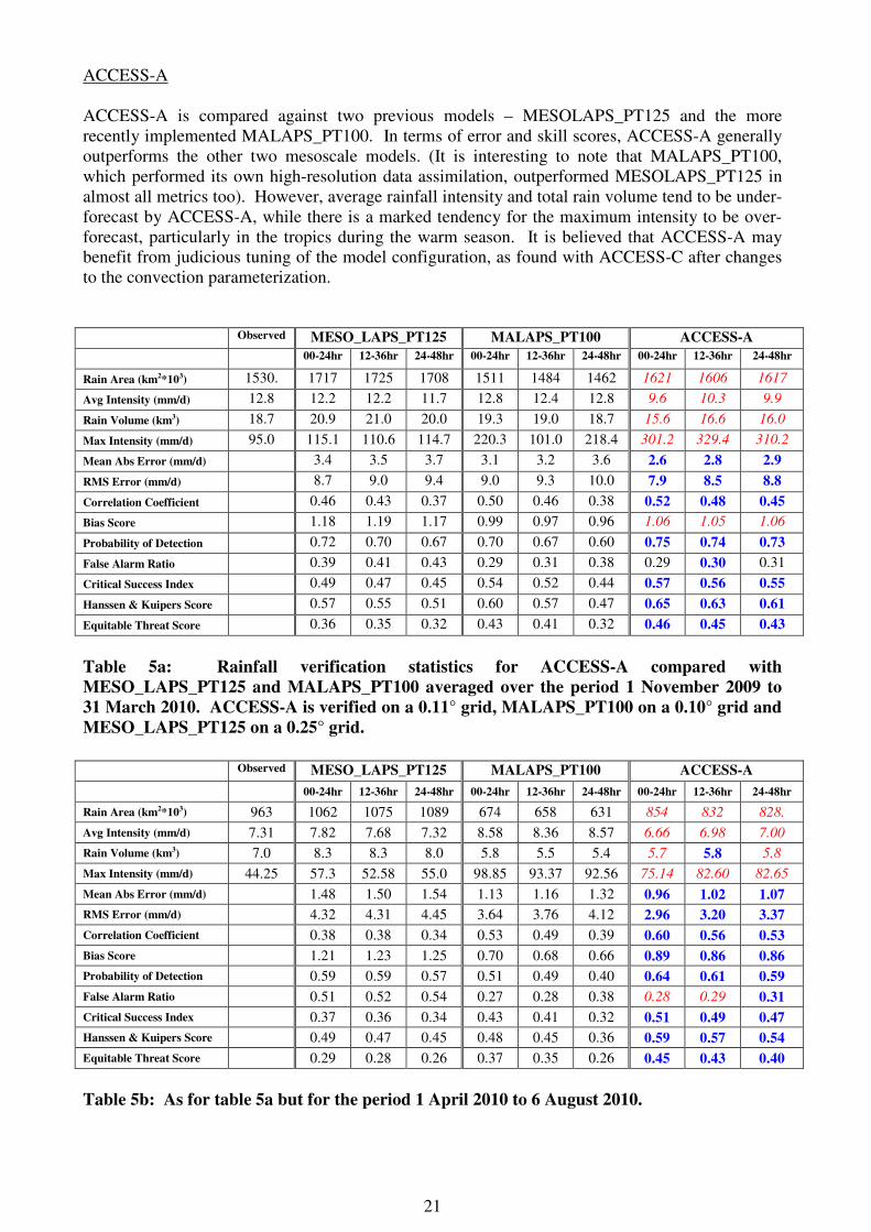
ACCESS-A is compared against two previous models – MESOLAPS_PT125 and the more

recently implemented MALAPS_PT100. In terms of error and skill scores, ACCESS-A generally

outperforms the other two mesoscale models. (It is interesting to note that MALAPS_PT100,

which performed its own high-resolution data assimilation, outperformed MESOLAPS_PT125 in

almost all metrics too). However, average rainfall intensity and total rain volume tend to be under-

forecast by ACCESS-A, while there is a marked tendency for the maximum intensity to be over-

forecast, particularly in the tropics during the warm season. It is believed that ACCESS-A may

benefit from judicious tuning of the model configuration, as found with ACCESS-C after changes

to the convection parameterization.

Observed MESO_LAPS_PT125 MALAPS_PT100 ACCESS-A

00-24hr 12-36hr 24-48hr 00-24hr 12-36hr 24-48hr 00-24hr 12-36hr 24-48hr

Rain Area (km2*103) 1530. 1717 1725 1708 1511 1484 1462 1621 1606 1617

Avg Intensity (mm/d) 12.8 12.2 12.2 11.7 12.8 12.4 12.8 9.6 10.3 9.9

Rain Volume (km3) 18.7 20.9 21.0 20.0 19.3 19.0 18.7 15.6 16.6 16.0

Max Intensity (mm/d) 95.0 115.1 110.6 114.7 220.3 101.0 218.4 301.2 329.4 310.2

Mean Abs Error (mm/d) 3.4 3.5 3.7 3.1 3.2 3.6 2.6 2.8 2.9

RMS Error (mm/d) 8.7 9.0 9.4 9.0 9.3 10.0 7.9 8.5 8.8

Correlation Coefficient 0.46 0.43 0.37 0.50 0.46 0.38 0.52 0.48 0.45

Bias Score 1.18 1.19 1.17 0.99 0.97 0.96 1.06 1.05 1.06

Probability of Detection 0.72 0.70 0.67 0.70 0.67 0.60 0.75 0.74 0.73

False Alarm Ratio 0.39 0.41 0.43 0.29 0.31 0.38 0.29 0.30 0.31

Critical Success Index 0.49 0.47 0.45 0.54 0.52 0.44 0.57 0.56 0.55

Hanssen & Kuipers Score 0.57 0.55 0.51 0.60 0.57 0.47 0.65 0.63 0.61

Equitable Threat Score 0.36 0.35 0.32 0.43 0.41 0.32 0.46 0.45 0.43

Table 5a: Rainfall verification statistics for ACCESS-A compared with

MESO_LAPS_PT125 and MALAPS_PT100 averaged over the period 1 November 2009 to

31 March 2010. ACCESS-A is verified on a 0.11° grid, MALAPS_PT100 on a 0.10° grid and

MESO_LAPS_PT125 on a 0.25° grid.

Observed MESO_LAPS_PT125 MALAPS_PT100 ACCESS-A

00-24hr 12-36hr 24-48hr 00-24hr 12-36hr 24-48hr 00-24hr 12-36hr 24-48hr

Rain Area (km2*103) 963 1062 1075 1089 674 658 631 854 832 828.

Avg Intensity (mm/d) 7.31 7.82 7.68 7.32 8.58 8.36 8.57 6.66 6.98 7.00

Rain Volume (km3) 7.0 8.3 8.3 8.0 5.8 5.5 5.4 5.7 5.8 5.8

Max Intensity (mm/d) 44.25 57.3 52.58 55.0 98.85 93.37 92.56 75.14 82.60 82.65

Mean Abs Error (mm/d) 1.48 1.50 1.54 1.13 1.16 1.32 0.96 1.02 1.07

RMS Error (mm/d) 4.32 4.31 4.45 3.64 3.76 4.12 2.96 3.20 3.37

Correlation Coefficient 0.38 0.38 0.34 0.53 0.49 0.39 0.60 0.56 0.53

Bias Score 1.21 1.23 1.25 0.70 0.68 0.66 0.89 0.86 0.86

Probability of Detection 0.59 0.59 0.57 0.51 0.49 0.40 0.64 0.61 0.59

False Alarm Ratio 0.51 0.52 0.54 0.27 0.28 0.38 0.28 0.29 0.31

Critical Success Index 0.37 0.36 0.34 0.43 0.41 0.32 0.51 0.49 0.47

Hanssen & Kuipers Score 0.49 0.47 0.45 0.48 0.45 0.36 0.59 0.57 0.54

Equitable Threat Score 0.29 0.28 0.26 0.37 0.35 0.26 0.45 0.43 0.40


22

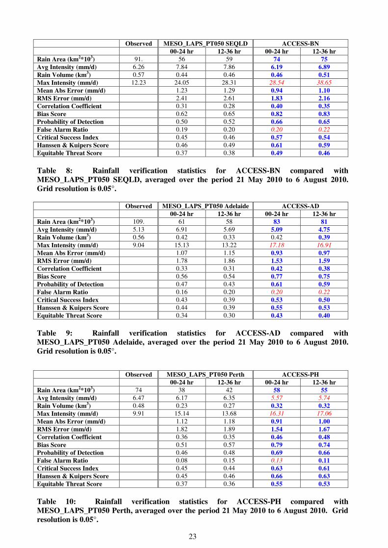
ACCESS-C

Tables 6 to 10 show the RAINVAL results for the various 5km ACCESS-C models compared with

the corresponding 5km MESOLAPS models for the period from 21 May 2010 to 6 Aug 2010.

Generally, ACCESS-C verifies very well and outperforms the equivalent MESOLAPS forecasts in

all metrics except for maximum rainfall intensity, which ACCESS-C tends to over-predict (as does

MESOLAPS although to a lesser extent). Total rain area and volume tend to be under-predicted

by ACCESS but performance is still better than MESOLAPS for these metrics.

Observed MESO_LAPS_PT050 VICTAS ACCESS-VT

00-24 hr 12-36 hr 00-24 hr 12-36 hr

Rain Area (km2*10

3) 180. 118 131 145 151

Avg Intensity (mm/d) 6.67 7.02 6.99 6.77 6.68

Rain Volume (km3) 1.20 0.83 0.92 0.99 1.01

Max Intensity (mm/d) 20.28 31.26 31.89 41.26 42.11

Mean Abs Error (mm/d) 1.58 1.70 1.32 1.44

RMS Error (mm/d) 2.91 3.05 2.49 2.69

Correlation Coefficient 0.51 0.49 0.60 0.57

Bias Score 0.65 0.73 0.81 0.84

Probability of Detection 0.56 0.60 0.70 0.70

False Alarm Ratio 0.14 0.18 0.14 0.17

Critical Success Index 0.51 0.53 0.63 0.61

Hanssen & Kuipers Score 0.51 0.53 0.64 0.62

Equitable Threat Score 0.39 0.39 0.50 0.48

Table 6: Rainfall verification statistics for ACCESS-VT compared with

MESO_LAPS_PT050 VICTAS, averaged over the period 21 May 2010 to 6 August 2010.

Grid resolution is 0.05°.

Observed MESO_LAPS_PT050 Sydney ACCESS-SY

00-24 hr 12-36 hr 00-24 hr 12-36 hr

Rain Area (km2*10

3) 111. 70 78 90 91


Rain Volume (km3) 0.89 0.64 0.70 0.72 0.73



RMS Error (mm/d) 3.71 3.81 2.81 3.10


Bias Score 0.63 0.70 0.82 0.83






Table 7: Rainfall verification statistics for ACCESS-SY compared with

MESO_LAPS_PT050 SYDNEY, averaged over the period 21 May 2010 to 6 August 2010.


23

Observed MESO_LAPS_PT050 SEQLD ACCESS-BN

00-24 hr 12-36 hr 00-24 hr 12-36 hr

Rain Area (km2*10

3) 91. 56 59 74 75


Rain Volume (km3) 0.57 0.44 0.46 0.46 0.51



RMS Error (mm/d) 2.41 2.61 1.83 2.16


Bias Score 0.62 0.65 0.82 0.83






Table 8: Rainfall verification statistics for ACCESS-BN compared with

MESO_LAPS_PT050 SEQLD, averaged over the period 21 May 2010 to 6 August 2010.


Observed MESO_LAPS_PT050 Adelaide ACCESS-AD

00-24 hr 12-36 hr 00-24 hr 12-36 hr

Rain Area (km2*10

3) 109. 61 58 83 81


Rain Volume (km3) 0.56 0.42 0.33 0.42 0.39



RMS Error (mm/d) 1.78 1.86 1.53 1.59


Bias Score 0.56 0.54 0.77 0.75






Table 9: Rainfall verification statistics for ACCESS-AD compared with

MESO_LAPS_PT050 Adelaide, averaged over the period 21 May 2010 to 6 August 2010.


Observed MESO_LAPS_PT050 Perth ACCESS-PH

00-24 hr 12-36 hr 00-24 hr 12-36 hr

Rain Area (km2*10

3) 74 38 42 58 55


Rain Volume (km3) 0.48 0.23 0.27 0.32 0.32



RMS Error (mm/d) 1.82 1.89 1.54 1.67


Bias Score 0.51 0.57 0.79 0.74






Table 10: Rainfall verification statistics for ACCESS-PH compared with

MESO_LAPS_PT050 Perth, averaged over the period 21 May 2010 to 6 August 2010. Grid

resolution is 0.05°.

24

8.4 Surface weather element verification

ACCESS-A mesoscale system

In the course of verifying the hourly high-resolution Mesoscale Surface Analysis System (MSAS),

short range (hours +3 to +8) ACCESS-A and MESOLAPS model forecasts of selected surface

weather elements have been validated against all available Australian surface observations for the

period 10 to 18 July 2010 by Tomasz Glowacki of CAWCR. Some results of that work are

presented in Figure 13 which shows forecast RMS error and bias of mean sea level pressure,

screen level temperature, screen level dewpoint temperature and the zonal and meridional

components of the 10m wind.

For MSAS, a mesoscale model (previously MESOLAPS but now ACCESS-A) is used to provide

the first guess for the surface analysis. At any particular hour of the day the latest available model

forecast for that time is used, so typically observations at 03,04,05,06,07,08 UTC were compared

against the +3,+4,+5,+6,+7,+8 hour forecasts from the 00Z model, whereas observations at

09,10,11,12,13,14 UTC are compared with the +3,+4,+5,+6,+7,+8 hour forecasts from the 06Z

model run, etc. The plots in Figure 7 therefore give an estimate of the average errors and biases

found in the short term forecasts available throughout the day.

It can be seen that, in general, ACCESS-A shows smaller RMS errors than MESOLAPS for most

hours of the day, particularly for the MSLP, temperature and wind fields. Biases are also

significantly better for most fields throughout the day, except for the 10m zonal wind component

which tends to display a slightly greater (0.1 to 0.2 m/s) negative bias than MESOLAPS during the

evening and overnight.

25

MSLP

0

0.4

0.8

1.2

1.6

2

0 1 2 3 4 5 6 7 8 9 10 11 12 13 14 15 16 17 18 19 20 21 22 23

hour ( UTC )

rmse ( h

Pa )

MSLP

-1

-0.5

0

0.5

1

1.5

0 1 2 3 4 5 6 7 8 9 10 11 12 13 14 15 16 17 18 19 20 21 22 23

hour ( UTC )

bia

s ( h

Pa )

PT

0

0.5

1

1.5

2

2.5

3

0 1 2 3 4 5 6 7 8 9 10 11 12 13 14 15 16 17 18 19 20 21 22 23

hour ( UTC )

rmse ( d

eg C

)

PT

-0.4

0

0.4

0.8

1.2

1.6

0 1 2 3 4 5 6 7 8 9 10 11 12 13 14 15 16 17 18 19 20 21 22 23

hour ( UTC )

bia

s ( d

eg C

)

D 2

0

0.5

1

1.5

2

2.5

3

0 1 2 3 4 5 6 7 8 9 10 11 12 13 14 15 16 17 18 19 20 21 22 23

hour ( UTC )

rmse ( d

eg C

)

D 2

-1.2

-0.8

-0.4

0

0.4

0.8

0 1 2 3 4 5 6 7 8 9 10 11 12 13 14 15 16 17 18 19 20 21 22 23

hour ( UTC )

bia

s ( d

eg C

)

U 10

0

0.5

1

1.5

2

2.5

3

0 1 2 3 4 5 6 7 8 9 10 11 12 13 14 15 16 17 18 19 20 21 22 23

hour ( UTC )

rmse ( m

/ s

ec )

U 10

-0.3

-0.2

-0.1

0

0.1

0.2

0.3

0.4

0.5

0 1 2 3 4 5 6 7 8 9 10 11 12 13 14 15 16 17 18 19 20 21 22 23

hour ( UTC )

bia

s ( m

/ s

ec )

V 10

0

0.5

1

1.5

2

2.5

3

0 1 2 3 4 5 6 7 8 9 10 11 12 13 14 15 16 17 18 19 20 21 22 23

hour ( UTC )

rmse ( m

/ s

ec )

V 10

-0.2

-0.1

0

0.1

0.2

0.3

0.4

0.5

0.6

0 1 2 3 4 5 6 7 8 9 10 11 12 13 14 15 16 17 18 19 20 21 22 23

hour ( UTC )

bia

s ( m

/ s

ec )

Figure 13: Comparison of hourly forecast RMSE (left) and bias (right) for ACCESS-A

(green) and MESOLAPS (black) against all available Australian surface observations of

surface weather elements Mean Sea Level pressure (mslp), screen level temperature (PT),

screen level dewpoint temperature( D2), zonal 10m wind component (U10), meridional 10m

wind component (V10). Results are averaged over the period 10 to 18 July 2010.

26

8.5 Known ACCESS problems

Excessive screen level specific humidities

Forecasters have noticed excessive values of the screen level (1.5m) specific humidity diagnostic

in ACCESS during situations of very low wind speeds just after sunset. From analysis of a number

of case studies, lines or confined areas of high specific humidity values tend to occur over inland

NSW and across inland WA associated with regions of surface convergence (trough lines) where

10m wind speed falls below 2m/s. Transition to excessive values can be rapid and severity is

greatest usually just after sunset (07-10Z in eastern states) and then dies down overnight after

about 12-14Z.

Currently, the operational display tool “Kenny” has an option of looking at the 20m humidity value

as an alternative to the screen level value. CAWCR scientists are currently testing a new

diagnostic algorithm for 1.5m specific humidity which better captures the decoupling of the

boundary layer during the evening transition period but until it becomes operational a crude

estimate of its effect can be made by taking a value halfway between the current 1.5m (screen

level) and the 20m value. It should be noted that the specific humidity errors are associated with

the calculation of the diagnostic only and are not used in the precipitation calculations. Currently,

all screen level (1.5m) diagnostics such as specific humidity, dew point and temperature should be

treated with caution as they are all calculated with the same coefficient in the model.

Noisy MSLP fields in ACCESS-C

It has been noted that occasionally there can be distortions which appear to be unrealistic in the

MSLP patterns over the Alps of SE Australia in the forecasts from ACCESS-C in strong NW to

SW flow. Nevertheless, it is clear that transitioning from the 37 km and 12 km grid spacing of

ACCESS-R and ACCESS-A respectively down to a 5km grid spacing in ACCESS-C allows an

improved definition of the major mesoscale topographic features and their corresponding

atmospheric circulations. Consequently, by decreasing the grid spacing as in ACCESS-C more

detailed atmospheric structure becomes evident. In addition, preliminary examination of the

boundary layer wind fields in strong westerly flow over SE Australia indicates that the wind fields

appear to be realistic.

The ACCESS-C systems are nested inside the regional ACCESS model ("ACCESS-R"), and hence

are expected to benefit from its already-established significantly improved forecast accuracy. The

ACCESS-C systems are also much less diffusive than their MESOLAPS counterparts - in fact,

they have no explicit diffusion applied at all, this despite the fact that they are using more accurate

(less smoothed) surface topography than the MESOLAPS systems. As a result, they produce more

finely detailed forecasts of MSLP, boundary-layer winds and rainfall despite the fact that the grid

resolution has not been increased. Whilst the interpretation of this additional detail will require

considerable care on the part of the forecaster, there is the potential for these systems to provide

additional value in alerting the forecaster to the possibility of significant, rapidly evolving,

features, such as rainfall.

27

Excessive daily rainfall rates in ACCESS-C and ACCESS-A

As discussed in section 8, there is a general tendency for the ACCESS models to under-forecast

the average rainfall intensity and total rain volume – this characteristic trait is seen in all ACCESS

models and resolutions. For the higher resolution ACCESS-A and C models there is also a

tendency for the maximum intensity to be over-predicted, particularly in the tropics during the

warm season. Nevertheless, ACCESS forecasts overall tend to be more skillful than the forecasts

from the corresponding GASP/LAPS etc models.

Boundary effects in regional models

All models except ACCESS-G use boundary conditions that are provided by a coarser resolution

ACCESS model, e.g. ACCESS-R and T are nested inside the previous run of ACCESS-G, while

ACCESS-A and C are nested inside the concurrent run of ACCESS-R (c.f. Table 2). Some

noticeable effects have been seen near the boundaries of the regional models, particularly in the

rainfall field. This is illustrated in figure 14 which shows examples of the 24-hour accumulated

precipitation field for two particular dates of some ACCESS runs when very sharp cutoffs were

noticed in the rainfall near the southern boundaries. These effects have been reported to CAWCR

for their investigation. In the meantime, users are advised to treat forecast fields near the model

boundaries with caution.

Figure 14. Examples of ACCESS 24-hour accumulated precipitation forecasts showing

anomalous rainfall amounts near the model boundaries. ACCESS-T (left) contour levels are

1,2,5,10,20,50,100 mm/day. An ACCESS-C (Adelaide) forecast is shown on the right.

9. Model output data

Model forecast data is written out from the UM in a proprietary UKMO format. The raw model

files are then converted to GRIB edition 1 before being stored in the MARS archival and retrieval

system. The GRIB files can be converted to NetCDF if required. A proposed upgrade to use GRIB

edition 2 will be investigated in 2011.

The “raw” model-level data is on a horizontally and vertically staggered grid (c.f. section 4 and the

appendix) and can be difficult to use without specially designed software. Most users will instead

opt to use data that has been “de-staggered”, i.e. interpolated to a common grid. Horizontally and

vertically de-staggered data with all fields interpolated to the model theta levels (with lower levels

28

at 20m, 80m, 180m etc, refer to Table 13 in the appendix for a full list of model theta levels) will

be made available to users.

As mentioned in section 4 and described in detail in the appendix, the model vertical levels are

“hybrid height” levels which approximate a constant height above terrain in the low levels, and

blend to constant heights above MSL above approximately 30km. For the first year or so, to

facilitate interfacing to legacy downstream systems, output interpolated to sigma levels

(sigma=P/Psurface) similar to the output from the previous MESOLAPS systems, will also be made

available. However, users should be aware that the conversion of the hybrid height levels to sigma

levels introduces interpolation errors. If possible, users of sigma level data should convert their

applications to use the hybrid model-level data instead.

Details of model field output frequency and the commencement date of the operational MARS

historical archive for each ACCESS system are shown in Table 11.

System Single-level field output

frequency

Upper-level field output

frequency

MARS archive

commencement

ACCESS-G 3-hourly out to +240 hours 3-hourly out to +120 hours, then

6-hourly out to +240 hours 27 Aug 2009

ACCESS-R 1-hourly out to +72 hours 3-hourly out to +72 hours 23 Aug 2009

ACCESS-T 1-hourly out to +72 hours 3-hourly out to +72 hours 18 Sep 2009

ACCESS-A 1-hourly out to +48 hours 1-hourly* out to +48 hours

(* due to resource limitations,

most upper fields can only be

distributed 3-hourly)

5 Nov 2009

ACCESS-C 1-hourly out to +36 hours 1-hourly out to +36 hours 21 May 2010

Table 11: Frequency of ACCESS model output and the commencement date of the

operational MARS historical archive for each system.

10. Output product availability

Graphical products

Graphical displays of ACCESS forecast fields are available on the Bureau of Meteorology’s

external website at http://www.bom.gov.au/australia/charts/viewer/. By default this page displays

a variety of ACCESS-R surface and upper levels fields over the Australian regional domain at 3-

hourly intervals out to the +72 hour (i.e. day 3) forecast period, followed by 6-hourly ACCESS-G

fields for forecast periods out to day 7. A screenshot of this web-based chart viewer is shown in

Figure 14. A dropdown menu allows the display of other ACCESS models over a variety of

domains.

For many years the Bureau has produced as series of black & white “difacs” charts to display

fields from our NWP models. It is felt that many of these charts are now redundant and can be

replaced by the new colour charts mentioned above. Registered user web pages that link to the old

difacs charts will be modified to point to new colour ACCESS charts. A limited number of black

& white charts required for marine and radiofax distribution will be retained. Users who require

ongoing provision of other difacs charts should contact the Bureau as soon as possible.

29

Figure 15. Screenshot of the web-based interactive ACCESS chart viewer for external users.

Gridded data

Gridded data from the various ACCESS systems are available in GRIB-1 and NetCDF formats for

registered users. Details of subscription fees and download costs will be made available soon at

http://reg.bom.gov.au/other/charges.shtml. Individual data files correspond to collections of data

valid at a single forecast time-step and include:

• Single-level fields interpolated to a single uniform (horizontally destaggered) grid

• Multi-level fields interpolated to selected pressure levels on a single uniform (destaggered)

grid

• Multi-level fields on the model native “theta” vertical coordinates, interpolated to a single

uniform (horizontally destaggered) grid. For convenience, the wind field components have

also been interpolated to the model “theta” levels, although the horizontally de-staggered

wind fields on the model “rho” vertical levels will also be made available for users who

specifically require them.

• Multi-level fields interpolated to sigma levels on a single uniform (destaggered) grid will

also be made available for a limited period of time to facilitate interfacing of ACCESS to

legacy downstream systems. The 29 sigma levels are similar to the levels output from the

previous MESOLAPS systems. However, users should be aware that the conversion of the

hybrid height levels to sigma levels introduces interpolation errors. If possible, users of

sigma level data should convert their applications to use the hybrid model-level data

instead.

30

• Multilevel fields on the “raw” model grid (i.e. staggered - horizontally and vertically) will

be made available upon request to advanced users who specifically require such data for

precision modelling work.

Further details of the ACCESS gridded products and product bundles, together with sample data

files, a description of the available fields contained within and associated grib table files are

available on the Bureau’s website at http://www.bom.gov.au/nwp/.

11. Future plans

• Operational implementation of ACCESS-TC before 2010/2011 cyclone season

• With the planned upgrade to APS1 in early 2011 the number of vertical levels for all

models will be increased to 70 and ACCESS-G will have an increased horizontal resolution

of N320 (~40 km). A subsequent further resolution increase to N512 (~25 km) is then

planned for APS2 expected in late 2011.

• In APS1, the ACCESS-R resolution will be increased to 0.11° (~12km) and ACCESS-R

will replace ACCESS-A completely.

• ACCESS-T is expected to be discontinued in APS1 (subject to satisfactory performance of

the N320 ACCESS-G in the tropics)

• Some adjustments and additions to the ACCESS-C domains may be included in APS1.

• An “AGREPS” ACCESS Global and Regional Ensemble Prediction System is currently

undergoing development and testing in CAWCR. Operational implementation of this

system may be considered for APS2.

• Upgrade to version 7.5 of the UM and 26.1 of OPS and VAR in APS1

• Use of new observational data types including 1-hourly local AMVs, IASI, GPS and

WINDSAT scatterometer.

• A proposed upgrade to use GRIB version 2 data will be investigated in 2011.

• Improved data selection tools for external users of gridded model data are under

development. These tools will allow users to specify required levels, forecast hours and

domains.

• Improved graphical products.

12. Acknowledgements

The assistance of various CAWCR research staff in the provision of verification data is gratefully

acknowledged. In particular, thanks go to Chris Tingwell for the provision of the forecast versus

analysis verification statistics, Tomasz Glowacki and Tim Hume for the MSAS surface verification

statistics and Beth Ebert for assistance with the RAINVAL verification package. The model and

variational data assimilation descriptions in sections 4 and 5 were supplied by the CAWCR Earth

System Modelling staff. Thanks are also due for helpful comments provided by Vaughan Barras,

Peter Steinle and Gary Dietachmayer.

31

13. References

Arakawa, A. & Lamb, V. R. 1977: “Computational design of the basic dynamical processes of the

UCLA general circulation model”, Methods in Comp. Phys. 17, 174–265.

Charney, J. G. & Phillips, N. A. 1953: “Numerical integration of the quasi-geostrophic equations

for barotropic and simple baroclinic flows”, J. Meteor. 10, 71–99.

Grant, A. L. M., & Brown, A. R. 1999: “A similarity hypothesis for shallow-cumulus transports“

Quart. J. Roy. Meteor. Soc., 125, 1913–1936.

Gregory, D., & P.R. Rowntree 1990: “A mass flux convection scheme with representation of cloud

ensemble characteristics and stability-dependent closure”, Mon. Weather Rev., 118, 1483–1506.

Harris, B. A. & Kelly, G. 2001: “A satellite radiance-bias correction scheme for data assimilation”,

Quart. J. Roy. Meteor. Soc., 127, 1453-1468.

Lock A. P. 1998: “The Parameterization of entrainment in cloudy boundary layers”, Quart. J. Roy.

Meteor. Soc., 124, 2729-2753.

Lock A. P., Brown, A. R., Bush, M. R., Martin, G. M. & Smith, R. N. B. 2000: “A new boundary

layer mixing scheme. Part I: Scheme description and single-column Model”, Mon. Wea. Rev., 128,

3187-3199.

Louis, J. F. 1979: “A parametric model of vertical eddy fluxes in the atmosphere”, Boun.-Layer

Meteor., 17, 187-202.

Mass C. et al 2002: “Does increasing horizontal resolution produce more skillful forecasts? The

results of two years of real time weather prediction over the Pacific Northwest”, Bull. Am.

Meteorol. Soc., 83, no. 3, 407-430.

McBride, J. and Ebert, E. 2000: “Verification of Quantitative Precipitation Forecasts from

Operational Numerical Weather Prediction Models over Australia”, Weather and Forecasting 15,

103-121.

Puri, K. 2005: “Blueprint for ACCESS”, June 2005, Bureau of Meteorology planning document

available from http://www.accessimulator.org.au/file/blueprint_access20050630.doc

Puri, K. 2005: “Project Plan for ACCESS”, September 2005, Bureau of Meteorology planning

document available from http://www.accessimulator.org.au/file/projplan_access20050916.doc

Seaman, R. & Hart, T. 2003: “The history of PAOBs in the Bureau of Meteorology” Aust. Met.

Mag., 52, 241-250.

Smith, R.N.B. 1990: “A scheme for predicting layer clouds and their water contents in a general

circulation model”, Quart. J. Roy. Meteor. Soc.,116, 435-460.

Wilson, D.R. & Ballard, S.P. 1999: “A microphysically based precipitation scheme for the UK

Meteorological Office Unified Model”, Quart. J. Roy. Meteor. Soc.,125, 1607-36.

32

APPENDIX: Horizontal and vertical grid structure of the ACCESS model

The UM system uses an Arakawa C-grid in the horizontal and a Charney-Phillips grid in the

vertical. This results in fields located on different grids displaced by half a grid spacing in both

vertical (height) and horizontal (longitude and latitude) directions. The vertical levels consist of

interleaved “theta” and “rho” levels, so named after the main variables stored on them. This

staggered arrangement of fields is designed to allow for accurate finite differencing; the exact

arrangement is detailed in table 12 and illustrated in figure 16 below.

Variable Grid location (longitude, latitude, height)

Pressure, Density i j k

Temperature, Humidity, Vertical Wind Speed i j k ± ½

Zonal Wind Speed i ± ½ j k

Meridional Wind Speed i j ± ½ k

Table 12: Grid positions of variables neighbouring a central point (i, j, k) in grid length units.

Figure 16: Model grid arrangement as per table 12. This staggered grid pattern has dimensions

of one grid unit on all sides and is repeated in all three dimensions to form the entire model grid.

The ACCESS models are configured such that each grid point in the horizontal is spaced a

constant latitude and longitude increment apart from adjacent grid points. The vertical levels are

constructed in a “hybrid” fashion so they conform to terrain heights near the surface and become

constant height surfaces in the upper atmosphere as per equation 1 (illustrated in figure 17).

≥

<−+=

Interfaceiforz

Interfaceiforzzz

Ti

Interface

i

sTi

i

η

η

ηη

2)1( Equation 1

where zi is the height above mean-sea-level (MSL) of model level i at a particular latitude and

longitude, zT is a constant corresponding to the height above MSL at the top of the model, zs is the

33

terrain height above MSL at the particular latitude and longitude, ηi is the “eta” value of model

level i and ηInterface is the “rho”-level η value at i = Interface. The current 50-level UM systems

running in NMOC have zT = 62918.64699999984 m, Interface = 30, and ηi values as per table 14.

It should also be noted that the UM assumes a spherical earth with radius (to MSL) equal to the

mean radius of the planet (6371229 m).

Users interested in model levels near the surface should be aware that the near surface levels are

not exactly terrain following but tend to be “compressed” somewhat over surface topography– the

magnitude of this compression is a consequence of the use of “flat” levels in the upper domain of

the model. Examples of this variation of model level height for 4 different underlying topographic

surface heights for the first 3 model “rho” levels are shown in table 13.

Level index η (rho level) Surface

topography

height (m)

Level height

above sea

level (m)

Level height

above surface

topography (m)

Level deviation

from zero

topography

case (m)

Percentage

deviation

from zero

topography

case (%)

0 130.00 130.00 0.00 0.0%

500 622.56 122.56 -7.44 -5.7%

1000 1115.12 115.12 -14.88 -11.4% 3 0.0020662

1500 1607.68 107.68 -23.32 -17.2%

0 50.00 50.00 0.00 0.0%

500 547.13 47.13 -2.87 -5.7%

1000 1044.27 44.27 -5.73 11.5% 2 0.0007947

1500 1541.40 41.40 -8.60 -17.2%

0 10.00 10.00 0.00 0.0%

500 509.42 9.42 -0.58 -5.8%

1000 1008.85 8.85 -1.15 -11.5% 1 0.0001589

1500 1508.28 8.28 -1.72 -17.2%

Table 13: Variation of model “rho” level heights above surface topography.

Figure 17: Schematic of hybrid coordinate system used in ACCESS UM models

34

Level index η (at theta levels) Height (m) η (at rho levels) Height (m)

50 1.0000000 62918 0.9531141 59968

49 .9062281 57018 0.8662998 54506

48 .8263715 51994 0.7923848 49855

47 .7583982 47717 0.7294412 45895

46 .7004842 44073 0.6757434 42516

45 .6510026 40960 0.6297574 39623

44 .6085122 38286 0.5901292 37130

43 .5717462 35973 0.5556734 34962

42 .5396007 33951 0.5253624 33055

41 .5111240 32159 0.4983146 31353

40 .4855051 30547 0.4737836 29810

39 .4620621 29072 0.4511468 28385

38 .4402316 27698 0.4298941 27048

37 .4195567 26398 0.4096167 25772

36 .3996766 25147 0.3899956 24538

35 .3803146 23929 0.3707909 23329

34 .3612672 22730 0.3518300 22136

33 .3423928 21543 0.3329966 20951

32 .3236004 20360 0.3142195 19770

31 .3048386 19180 0.2954611 18590

30 .2860837 18000 0.2767065 17410

29 .2673293 16820 0.2582700 16250

28 .2492107 15680 0.2404693 15130

27 .2317278 14580 0.2233042 14050

26 .2148807 13520 0.2067749 13010

25 .1986692 12500 0.1908814 12010

24 .1830936 11520 0.1756236 11050

23 .1681536 10580 0.1610016 10130

22 .1538495 9680 0.1470152 9250

21 .1401810 8820 0.1336647 8410

20 .1271483 8000 0.1209498 7610

19 .1147514 7220 0.1088707 6850

18 .1029901 6480 0.0974274 6130

17 .0918647 5780 0.0866198 5450

16 .0813749 5120 0.0764479 4810

15 .0715209 4500 0.0669118 4210

14 .0623027 3920 0.0580114 3650

13 .0537202 3380 0.0497468 3130

12 .0457734 2880 0.0421179 2650

11 .0384624 2420 0.0351247 2210

10 .0317871 2000 0.0287673 1810

9 .0257475 1620 0.0230456 1450

8 .0203437 1280 0.0179597 1130

7 .0155757 980 0.0135095 850

6 .0114433 720 0.0096951 610

5 .0079468 500 0.0065164 410

4 .0050859 320 0.0039734 250

3 .0028608 180 0.0020662 130

2 .0012715 80 0.0007947 50

1 .0003179 20 0.0001589 10

Table 14: Model vertical levels and equivalent heights in the absence of topography. The model

level structure used in the UM uses a “hybrid” coordinate system which is split between terrain-

following quadratic η surfaces near the surface and flat linear η surfaces above a specified level.

Currently level 30 is the lowest “constant height” rho level in the UM configuration used in NMOC.

Operational implementation of the ACCESS Numerical Weather Prediction systems · ·...

Documents

Transcript of Operational implementation of the ACCESS Numerical Weather Prediction systems · ·...