Title 3D Delaunay triangulation of non-uniform point distributions

Author(s) Lo, SH

Citation Finite Elements in Analysis and Design, 2014, v. 90, p. 113-130

Issued Date 2014

URL http://hdl.handle.net/10722/210702

Rights

Posting accepted manuscript (postprint):© 2014. This manuscript version is made available under the CC-BY-NC-ND 4.0 license http://creativecommons.org/licenses/by-nc-nd/4.0/; This work is licensed under a Creative CommonsAttribution-NonCommercial-NoDerivatives 4.0 InternationalLicense.

1

3D Delaunay triangulation of non-uniform point distributions

S.H. Lo

Department of Civil Engineering, the University of Hong Kong, Pokfulam, Hong Kong

(email: hreclsh@hku.hk)

ABSTRACT

In view of the simplicity and the linearity of regular grid insertion, a multi-grid insertion scheme is proposed for the three-dimensional Delaunay triangulation of non-uniform point distributions by recursive application of the regular grid insertion to an arbitrary subset of the original point set. The fundamentals and difficulties of three-dimensional Delaunay triangulation of highly non-uniformly distributed points by the insertion method are reviewed. Current strategies and methods of point insertions for non-uniformly distributed spatial points are discussed. An enhanced kd-tree insertion algorithm with a specified number of points in a cell and its natural sequence derived from a sandwich insertion scheme is also presented.

The regular grid insertion, the enhanced kd-tree insertion and the multi-grid insertion have been rigorously studied with benchmark non-uniform distributions of 0.4 to 20 million points. It is found that the kd-tree insertion is more efficient in locating the base tetrahedron, but it is also more sensitive to the triangulation of non-uniform point distributions with a large amount of conflicting elongated tetrahedra. Including the grid construction time, multi-grid insertion is the most stable and efficient for all the uniform and non-uniform point distributions tested.

KEY WORDS: 3D Delaunay triangulation, non-uniform point distributions, regular grid, multi-grid, kd-tree insertions

2

1. INTRODUCTION

Based on a simple geometrical concept, Delaunay triangulation has important applications in many fields, including data visualization, terrain modeling, finite element mesh generation, surface reconstruction, bio-medical modeling from images and structural networking for arbitrary point sets, etc. [1,2] The popularity of Delaunay triangulation is attributed to its sound geometric properties as a dual of Voronoi tessellation and the speed with which it can be constructed in two and higher dimensions. In view of its diverse applications, many strategies for its construction have been proposed. In a paper by Su and Drydale [3], numerical tests of uniformly and non-uniformly distributed point sets on several Delaunay triangulation algorithms, namely, divide-and conquer, sweep line algorithms, incremental algorithms, a fast incremental construction algorithm, gift wrapping algorithms and convex hull based algorithms were carried out and their performance were compared.

With a rapid increase in the problem size from thousands of points to millions of points, it is necessary to devise ever more efficient schemes for the construct of Delaunay triangulations. Uniform or mildly non-uniform distribution point sets can be efficiently handled by the insertion scheme with the aid of a regular grid [4,5]. However, for highly non-uniform point distributions, the triangulation time may be many times more than that is required by a uniform point distribution. For the Delaunay triangulation of severe non-uniform point distributions, the complexity is nonlinear, such that the triangulation time may be excessively long for large point sets of millions of points.

Relative to a uniform point distribution, non-uniform point sets are significantly more difficult due to the following intrinsic properties of non-uniformly distributed points. (i) More efficient space control or partition has to be applied to highly non-uniform distributed points so that each partitioned cell contains roughly equal number of points. (ii) In the location of the base tetrahedron by the point insertion algorithm, the CPU time taken or the number of tetrahedra examined before the base tetrahedron could be determined is much longer than the case of uniform distribution as there are many pointed tetrahedra in the triangulation. (iii) In the creation of the insertion cavity upon the introduction of a new point, many tetrahedra have to be removed and reconstructed as long thin tetrahedra have large circumspheres, and a point can be connected to many distant points through long stretching tetrahedra. (iv) There are problems of numerical stability both in the determination of the base tetrahedron and in the verification of the empty circumsphere criterion, and more CPU time has to be allowed to exercise additional consistency checks and precautions.

In this paper, the difficulties of Delaunay triangulation of non-uniform point distributions by the insertion algorithm are discussed, and versatile enhanced kd-tree and multi-grid insertion schemes are proposed and tested with large sets of highly non-uniformly distributed points.

3

1.1 Delaunay triangulation

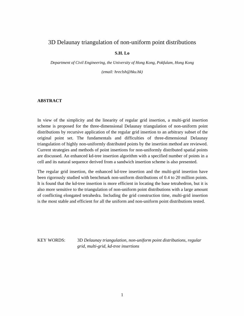
The Delaunay triangulation of a set of points on a plane is defined to be a triangulation such that the circumcircle of every triangle in the triangulation contains no point from the set in its interior. Such a triangulation exists for a given set of points, and it is the dual of the Voronoi tessellation. The triangulation is unique if the points are in general positions, i.e. no four points are cyclic. A triangle T is said to be Delaunay with respect to a point p if p does not lie inside the circumcircle of T. A triangle T in a triangulation of a set of points is call Delaunay triangle if T is Delaunay with respect to every point in the set. A triangulation of a set of points is called the Delaunay triangulation of the point set if every triangle in the triangulation is a Delaunay triangle as shown in Figure 1. The idea of Delaunay triangulation is very general, which can be easily extended to higher dimensions. For instance, the Delaunay triangulation in three dimensions is given by replacing triangle by tetrahedron, circle by sphere and 2D plane by 3D space. The following lemma provides the basis for many algorithms in the construction and verification of Delaunay triangulation.

Lemma of Delaunay [6]

Let T(S) be a triangulation of the point set S. The necessary and sufficient condition that no point of S is contained in the circumcircle of any triangle in the triangulation is that any two adjacent triangles in the triangulation are Delaunay with respect to each other’s vertices.

1.2 The Insertion Algorithm

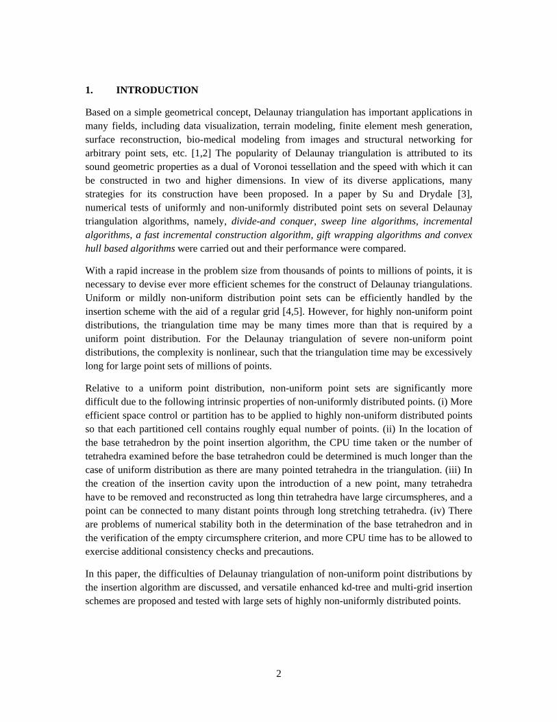
For the construction of Delaunay triangulation in three and higher dimensions, point insertion algorithm is the most popular, and many interesting methods have been proposed [2]. For a set of 3D points, the initial triangulation is a rectangular box consisting of five or six Delaunay tetrahedra large enough to contain all the given points as shown in Figure 2. The Delaunay triangulation is achieved by inserting points one by one into the initial triangulation. Each cycle of point

Figure 1. Delaunay triangulation of 14 points

Figure 2. Initial triangulation of five tetrahedra

Points to be inserted

4

insertion can be divided into three steps.

(i) For a newly inserted point, identify all the tetrahedra whose circumsphere contains the point in its interior. The CORE which is the cavity left behind upon removal of these tetrahedra forms a star-shaped insertion polyhedron.

(ii) Owing to the finite precision arithmetic, the triangulation facets on the boundary of the CORE have to be verified with the visibility check and corrected before they are connected with the inserted point to form tetrahedra.

(iii) The triangulation of the insertion polyhedron should be trivial. However, the adjacency relationship of the tetrahedra has to be established, which will be frequently referred to throughout the triangulation process.

The visibility test is a simple test to make sure that each triangular facet on the boundary of the CORE is visible to the insertion point P [2]. Once the boundary of the CORE is established by the sphere inclusion test, the CORE consists of all the non-Delaunay tetrahedra with respect to the insertion point P. One of the major difficulties in the implementation of the Delaunay triangulation by point insertion is to ensure consistency in the sphere inclusion test based on finite precision computations. An inconsistent decision in the sphere inclusion test may result in a disconnected CORE. Imprecise numerical calculation may also introduce tetrahedral with zero or negative volumes. Another type of degeneracy in three dimensions, which is due to the nature of Delaunay triangulation rather than the result of numerical error, can occur when four points are coplanar and cyclic. It is possible for these four points to form a tetrahedron of zero volume with non-zero edges and faces, which is known as sliver.

Using higher precision arithmetic can only postpone the problem to solve more cases which are near to degeneracy, but not to solve it completely. In 1992, Baker [26] proposed a solution in which tolerances depending on the values of the data and the machine precision are applied to all real number calculations. A more elegant solution is to use adaptive precision floating point arithmetic Shewchuk 1997 [27], Devillers and Preparata 1999 [28], which in theory would not introduce any numerical error for a wrong decision in case of nearly co-spherical points (i.e. five or more points on the circumsphere of a tetrahedron). However, exact integer arithmetic is not the panacea to all the problems, and the situation of exactly co-spherical points and natural degeneracy of sliver in Delaunay triangulation are still not resolved with robust geometric predicates Goliaz and Dutton 1997 [29]. Hardware and compilers may also prevent the algorithm from functioning properly, and even though a right decision is arrived for the sphere inclusion test, the connection is not unique and we do not have a systematic way in joining up any number of points on the surface of a sphere to produce a consistent triangulation, and sliver elements of zero or nearly zero volume will still be formed. Nevertheless, the visibility or the positive volume test appears to be simple and reliable in ensuring the CORE is connected and the volume of every tetrahedron is positive for a wide range of point distributions.

5

1.3 Efficient Insertion Scheme

When a new point p is inserted in a Delaunay triangulation, it is required to find all the tetrahedra whose circumsphere contains the point p. A simple method to determine those non-Delaunay tetrahedra is to scan through all the existing tetrahedra for those circumspheres containing the point p. However, a more efficient approach is to start with the tetrahedron which contains the inserted point p and find the others by means of the adjacency relationship. In this way, the boundary of the insertion polyhedron is given by the common faces of two tetrahedra for which one is positive in the sphere inclusion test while the other fails. The tetrahedron which contains the insertion point p is called the base, which is a core part of the insertion polyhedron.

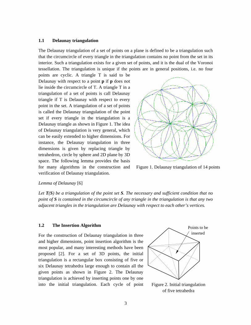
Although the end result of Delaunay triangulation of a set of n distinct points is independent of the order following which the points are inserted, the time taken or the complexity of triangulation is very sensitive to the sequence how points are processed. For the triangulation of randomly generated points by insertion, the complexity can vary from O(n) to O(n2) depending on the order of point insertion. For the 3D triangulation of 1 million points on a PC, if points are inserted following the natural order of point generation, triangulation time increased rapidly in a nonlinear manner with the number of points inserted as shown in Figure 3. On the other hand, also shown in Figure 3, if points are sorted and inserted more or less in a contiguous manner, a linear time relationship of the same set of points is resulted. For a 3D triangulation of 1 million points, it took 48 seconds for unsorted points but only 8 seconds for sorted points, and this quasi linear complexity can be sustained up to 50 million 3D points in 456 seconds.

Realizing that the point insertion sequence has a great impact on the time in locating the base tetrahedron, many schemes has been devised in determining how points should be ordered so as to reduce the time of triangulation [7-12]. This observation is in line with the second interesting remark under Notes and Discussion of the paper by Su and Drysdale [3], “A simple enhancement of the naïve incremental algorithm results in an easy to implement algorithm that runs in O(n) expected time for uniformly distributed sites. It is faster than previous incremental variants and competitive with other known algorithms for constructing the Delaunay triangulation for all but very bad sites”.

6

1.4 Fundamental and Strategies

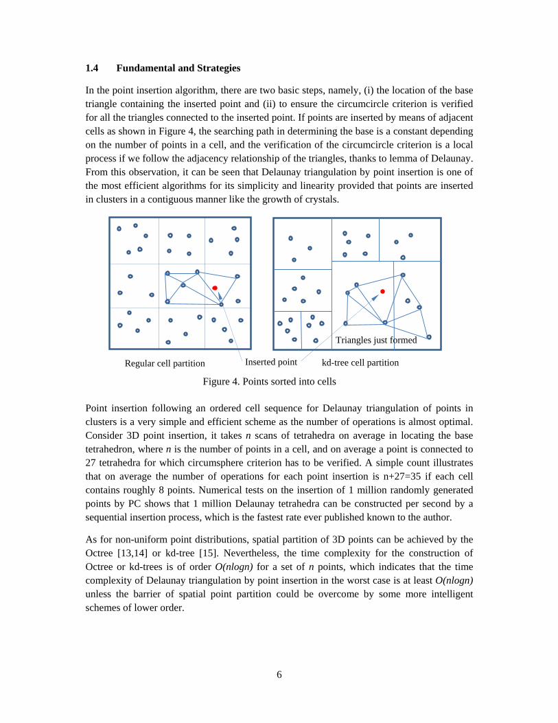
In the point insertion algorithm, there are two basic steps, namely, (i) the location of the base triangle containing the inserted point and (ii) to ensure the circumcircle criterion is verified for all the triangles connected to the inserted point. If points are inserted by means of adjacent cells as shown in Figure 4, the searching path in determining the base is a constant depending on the number of points in a cell, and the verification of the circumcircle criterion is a local process if we follow the adjacency relationship of the triangles, thanks to lemma of Delaunay. From this observation, it can be seen that Delaunay triangulation by point insertion is one of the most efficient algorithms for its simplicity and linearity provided that points are inserted in clusters in a contiguous manner like the growth of crystals.

Point insertion following an ordered cell sequence for Delaunay triangulation of points in clusters is a very simple and efficient scheme as the number of operations is almost optimal. Consider 3D point insertion, it takes n scans of tetrahedra on average in locating the base tetrahedron, where n is the number of points in a cell, and on average a point is connected to 27 tetrahedra for which circumsphere criterion has to be verified. A simple count illustrates that on average the number of operations for each point insertion is n+27=35 if each cell contains roughly 8 points. Numerical tests on the insertion of 1 million randomly generated points by PC shows that 1 million Delaunay tetrahedra can be constructed per second by a sequential insertion process, which is the fastest rate ever published known to the author.

As for non-uniform point distributions, spatial partition of 3D points can be achieved by the Octree [13,14] or kd-tree [15]. Nevertheless, the time complexity for the construction of Octree or kd-trees is of order O(nlogn) for a set of n points, which indicates that the time complexity of Delaunay triangulation by point insertion in the worst case is at least O(nlogn) unless the barrier of spatial point partition could be overcome by some more intelligent schemes of lower order.

Figure 4. Points sorted into cells

Regular cell partition kd-tree cell partition Inserted point

Triangles just formed

7

As for the identification of the insertion cavity, the number of tetrahedra checked and removed depends on the insertion sequence as well as the intrinsic characteristics and pattern of the point distributions. No theoretical results have been reported so far as how to devise an optimized order so as to minimize the number of conflicting tetrahedra in the entire triangulation process. While this is not an issue in uniform point distribution, for non-uniform point distributions, the total number of tetrahedra removed varies significantly with the order of point insertion. For highly non-uniform point distributions, over many parts, long thin tetrahedra with large circumscribing spheres exist. Upon the introduction of a newly inserted point near a cluster of elongated tetrahedra, a large number of tetrahedra have to be removed and reconstructed as shown in Figure 5. If points are to be inserted in a contiguous manner close to each other, the removal and reconstruction of elongated tetrahedra have to be repeated for each point insertion. Obviously, this is a rather time-consuming and perhaps unnecessary. The dilemma is that in order to reduce the time in searching for the base tetrahedron, points have to be inserted in a contiguous manner; however, in order not to remove and reconstruct elongated triangles in an excessive manner, points have to be inserted with sufficient separation. An effective algorithm ought to optimize both the search for the base and the conflicting tetrahedra in the creation of the insertion polyhedron (cavity).

Figure 5. Elongated tetrahedra over a spiral point distribution

8

2. REVIEW ON INSERTION SCHEMES

2.1 Random Order

In the earlier algorithms, points were introduced by the natural order (the order as their input) or sorted by a lexical axis-order [16]. This scheme has a tendency to produce intermediate triangulations of higher complexity than the final triangulation. The widely used random order was then devised to overcome the shortcomings of natural or lexical axis-order; it simply states that shuffle the points and insert them one by one [17]. There are several robust and efficient implementations of the incremental Delaunay triangulation construction based on random order point insertion, such as Clarkson's Hull [18] and that contained in the α -shapes software of Edelsbruner et al [19].

2.2 BRIO

Amenta N. et al presented a biased randomized insertion order (BRIO) in 2003[17]. Their argument was that since modern memory architecture is hierarchical and the paging policies favour programs that observe locality of reference, a major concern is cache coherence: a sequence of recent memory references should be clustered locally rather than randomly in the address space. A program implementing a randomized algorithm does not observe this rule and can be dramatically slowed down when its address space no longer fits in the main memory. The Biased Randomized Insertion Order (BRIO) preserves enough randomness in the input points so that the performance of a randomized incremental algorithm is unchanged but orders the points by spatial locality to improve cache coherence. However, from the reports of other researchers [8,9], the practical performance of BRIO is not promising. Indeed, Amenta et al considered BRIO a concept depending on the ever changing memory allocation schemes rather than a specific order, and BRIO could be implemented by merging with various insertion orders in a variety of ways.

2.3 Hilbert Curve

Recently, the pendulum seems to have swung back to the deterministic order. Due to the work of Liu and Snoeyink[8], Sheng Zhou and C.B. Jones[9], Samuel Hornus and J-D Boissonnat[10], Buchin, K [11,12], the space-filling curve orders are widely used for constructing Delaunay triangulations. Among them, the Hilbert curve order is considered to be the most efficient order because of its locality-preserving behaviour. In 2005, Liu and Snoeyink used the Hilbert curve order in their program tess3 for 3D Delaunay tessellation and compared it with qhull, CGAL2.4, pyramid and hull[8]. In their empirical comparisons, tess3 was the fastest for both uniform and non-uniform point distributions. Now the Hilbert curve order is also employed in the latest version of CGAL—CGAL3.7 [20], though mixing with the idea of BRIO in its implementation.

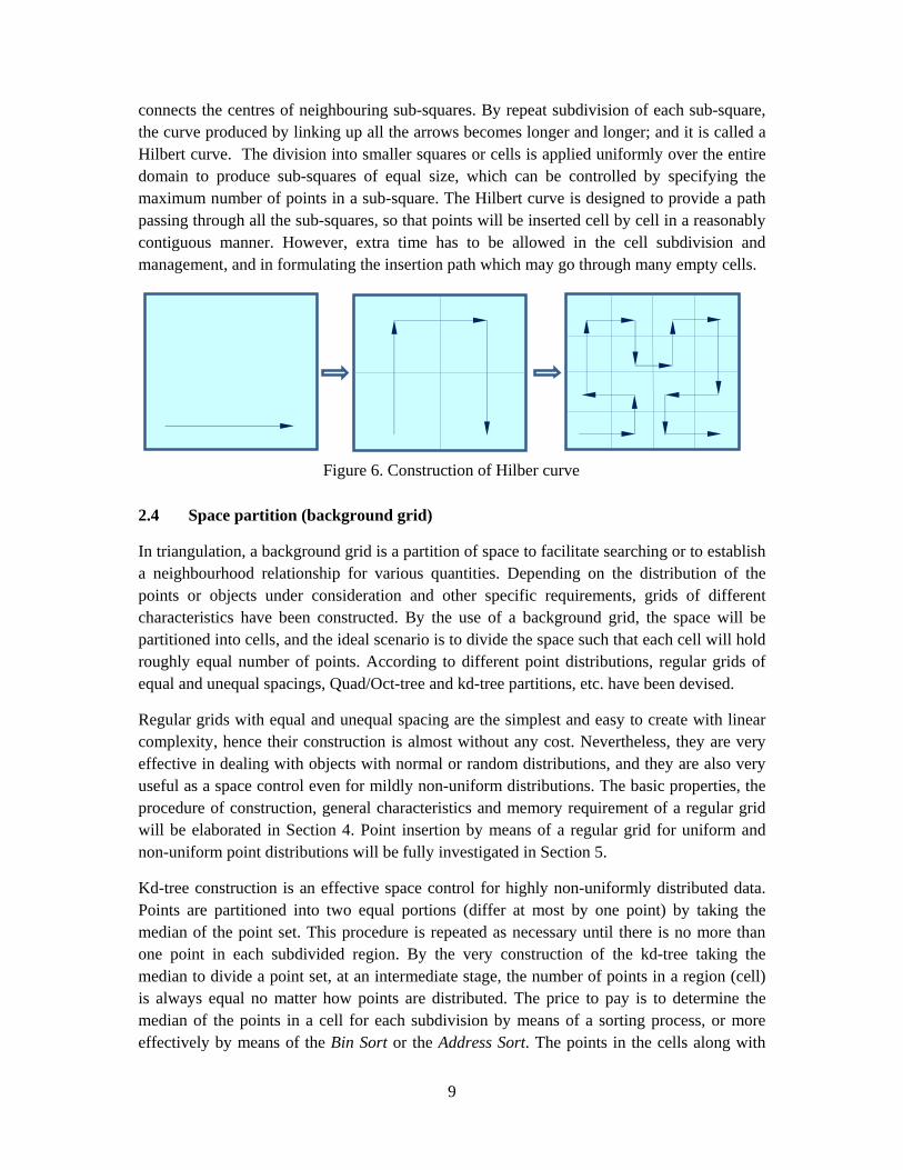
As a variant of the space-filling curve developed by Giuseppe Peano[21], the Hilbert curve is a fractal continuous space-filling curve first described by David Hilbert in 1891[22]. Its construction rule in the 2D case is shown in Figure 6. A square with an arrow is subdivided into four sub-squares. The ordering of the sub-squares is indicated by a blue arrow which

9

connects the centres of neighbouring sub-squares. By repeat subdivision of each sub-square, the curve produced by linking up all the arrows becomes longer and longer; and it is called a Hilbert curve. The division into smaller squares or cells is applied uniformly over the entire domain to produce sub-squares of equal size, which can be controlled by specifying the maximum number of points in a sub-square. The Hilbert curve is designed to provide a path passing through all the sub-squares, so that points will be inserted cell by cell in a reasonably contiguous manner. However, extra time has to be allowed in the cell subdivision and management, and in formulating the insertion path which may go through many empty cells.

2.4 Space partition (background grid)

In triangulation, a background grid is a partition of space to facilitate searching or to establish a neighbourhood relationship for various quantities. Depending on the distribution of the points or objects under consideration and other specific requirements, grids of different characteristics have been constructed. By the use of a background grid, the space will be partitioned into cells, and the ideal scenario is to divide the space such that each cell will hold roughly equal number of points. According to different point distributions, regular grids of equal and unequal spacings, Quad/Oct-tree and kd-tree partitions, etc. have been devised.

Regular grids with equal and unequal spacing are the simplest and easy to create with linear complexity, hence their construction is almost without any cost. Nevertheless, they are very effective in dealing with objects with normal or random distributions, and they are also very useful as a space control even for mildly non-uniform distributions. The basic properties, the procedure of construction, general characteristics and memory requirement of a regular grid will be elaborated in Section 4. Point insertion by means of a regular grid for uniform and non-uniform point distributions will be fully investigated in Section 5.

Kd-tree construction is an effective space control for highly non-uniformly distributed data. Points are partitioned into two equal portions (differ at most by one point) by taking the median of the point set. This procedure is repeated as necessary until there is no more than one point in each subdivided region. By the very construction of the kd-tree taking the median to divide a point set, at an intermediate stage, the number of points in a region (cell) is always equal no matter how points are distributed. The price to pay is to determine the median of the points in a cell for each subdivision by means of a sorting process, or more effectively by means of the Bin Sort or the Address Sort. The points in the cells along with

Figure 6. Construction of Hilber curve

10

the sequence of pivots of subdivision points form a sorted insertion order for the original point set. In a paper “A New Insertion Sequence for Incremental Delaunay Triangulation” by Liu et al [23], it is reported that kd-tree insertion is superior to Random, BRIO and Hilbert curve insertions up to 3 million 3D non-uniformly distributed points in various patterns such as cluster, disc, curved surface, line and spiral, etc.

In view of the better performance of kd-tree insertion over Random, BRIO and Hilbert curve insertions for a wide range of non-uniform point distributions, Random, BRIO and Hilbert curve will not be further explored in this paper. On the other hand, the regular grid insertion, the kd-tree insertion and its enhanced version developed in Section 3 will be rigorously tested against a wide range of data points from 0.4 to 20 million over a variety of non-uniform distribution patterns. In the light of the ease of construction of the regular grid and its linear characteristic for uniform distributed data, a new insertion scheme is proposed by recursive application of regular grid insertion to non-uniform distributed points partitioned into cells by regular grid or kd-tree. Exploiting the local homogeneity of non-uniformly distributed points, regular grid insertion is especially effective over uniform or non-uniform point distributions partitioned into tiny cells of a large number of points. The procedure of multi-grid insertion will be developed in Section 4, and the idea will be fully tested also in Section 5.

3. KD-TREE INSERTION SCHEME

3.1 Construction of Kd-tree

Based on the idea of space partition, a k-d tree (short form for k-dimensional tree) is a data structure in the form of a branching tree for organizing points in k-dimensional space. k-d trees provide a hierarchic spatial relationship between data points, which can be used to find nearest neighbours, locate points within a zone, and for other searching operations, such as construction and point insertion of Delaunay triangulation [24,25].

Construction of 2-d tree

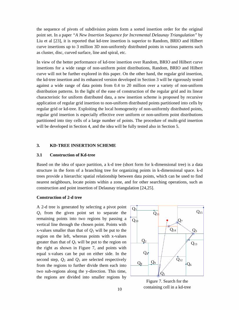
A 2-d tree is generated by selecting a pivot point Q1 from the given point set to separate the remaining points into two regions by passing a vertical line through the chosen point. Points with x-values smaller than that of Q1 will be put to the region on the left, whereas points with x-values greater than that of Q1 will be put to the region on the right as shown in Figure 7, and points with equal x-values can be put on either side. In the second step, Q2 and Q3 are selected respectively from the regions to further divide them each into two sub-regions along the y-direction. This time, the regions are divided into smaller regions by

Q1

Q2

Q3

Q4

Q5

Q6

Q7

Q8 Q9

Q10 Q11

Q12

Q13

Q14

Q15

Figure 7. Search for the containing cell in a kd-tree

11

horizontal lines passing points Q2 and Q3, so that roughly equal number of points are above and below the horizontal lines. Obviously, this subdivision process can be repeated by selecting one point from each region as pivot to create more sub-regions. As one point, the pivot, is taken away for each subdivision, for a set of N points there are N divisions and the space will be partitioned into N+1 regions.

A balanced tree will be resulted if the median is always selected as the pivot for each region sub-division, and in this case each region will contain approximately equal number of points (differ at most by one point). For a balanced tree construction, the level of subdivision can be calculated as the number of points in a region is reduced by half in each subdivision, and all the leaf nodes (nodes at the bottom of the tree) are about the same distance from the root. To construct a balanced k-d tree for a set of N points, the level of subdivision, L, is given by

.1)]([log)(log2 22 +=≥≥ ⇒⇒ NLNLNL where [ ] = Integral part Hence, L = 1, N = 1. L = 2, N = 2, 3. L = 3, N = 4, 5, 6, 7. L = 4, N = 8, 9, 10, 11, 12, 13, 14, 15, and so on. For a more symmetrical partition of space, the line of subdivision, vertical or horizontal, is rotated for each change of level of subdivision, i.e. L=1, vertical, L=2, horizontal, L=3, vertical, and so forth. Sequence of points A k-d tree can be conveniently defined by a proper sequencing of the given set of N points, P = {Pi, i = 1, N}. The following describes how a region Pi is divided into two sub-regions Pk and Pk+1. Find the median from Pi as pivot along the x-axis or y-axis depending on the level of subdivision. Set Qi = median, which divides Pi into Pk containing points on the left of Pi and Pk+1 containing points on the right of Pi. As Qi is the median in Pi, the number of points in Pk and the number of points in Pk+1 are given by

⎪⎩

⎪⎨

⎧ −

=⎪⎩

⎪⎨

⎧

−

−

= +.

2

,2

1

.12

,2

1

1evenisNifN

oddisNifN

NevenisNifN

oddisNifN

Ni

i

ii

k

ii

ii

k

where Ni = number of points in Pi. The subdivision will be carried out following the order of construction of the regions. As one point, Qi, is taken away for the subdivision of region Pi, the sequence {Qi, i = 1, N} will be established after exactly N subdivisions.

12

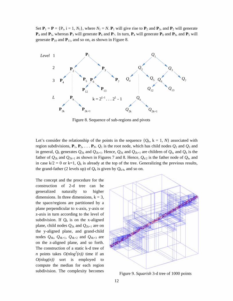
Set P1 = P = {Pi, i = 1, N1}, where N1 = N. P1 will give rise to P2 and P3, and P2 will generate P4 and P5, whereas P3 will generate P6 and P7. In turn, P4 will generate P8 and P9, and P5 will generate P10 and P11, and so on, as shown in Figure 8.

Let’s consider the relationship of the points in the sequence {Qk, k = 1, N} associated with region subdivisions, P1, P2, . . . PN. Q1 is the root node, which has child nodes Q2 and Q3 and in general, Qk generates Q2k and Q2k+1. Hence, Q2k and Q2k+1 are children of Qk, and Qk is the father of Q2k and Q2k+1 as shown in Figures 7 and 8. Hence, Qk/2 is the father node of Qk, and in case k/2 = 0 or k=1, Qk is already at the top of the tree. Generalizing the previous results, the grand-father (2 levels up) of Qk is given by Qk/4, and so on. The concept and the procedure for the construction of 2-d tree can be generalized naturally to higher dimensions. In three dimensions, k = 3, the space/regions are partitioned by a plane perpendicular to x-axis, y-axis or z-axis in turn according to the level of subdivision. If Qk is on the x-aligned plane, child nodes Q2k and Q2k+1 are on the y-aligned plane, and grand-child nodes Q4k, Q4k+1, Q4k+2 and Q4k+3 are on the z-aligned plane, and so forth. The construction of a static k-d tree of n points takes O(nlog2(n)) time if an O(nlog(n)) sort is employed to compute the median for each region subdivision. The complexity becomes

P1

P2 P3

P4 P5 P6 P7

Pk

P2k P2k+1

Q1

Q2 Q3

Q4 Q6 Q7

Qk

Q2k Q2k+1

Level 1

2

3

L k = 2L-1 . . . 2L - 1

Figure 8. Sequence of sub-regions and pivots

P12 P13 Q12 Q13

Q5

Figure 9. Squarish 3-d tree of 1000 points

13

O(nlog(n)) if a linear median finding algorithm is used [Lemaire 2000]. In the partition of regions, if the regions are cut along their longest side instead of rotating through the axes, the pattern and the performance of the k-d tree are quite different. The behaviour of the k-d trees are much better as points are more closely grouped together, and they are called squarish k-d trees [24]. It is noted that the construction of 2d-tree and 3d-tree takes roughly equal amount of CPU time, as the procedure is similar and the number of operations involved is exactly the same. A squarish 3d-tree of 1000 points distributed along a straight line is shown in Figure 9, in which small cells are found near the diagonal.

3.2 Kd-tree partition of points

A nice feature of kd-tree partition is that at any level of subdivision each region contains roughly equal number of points irrespective of the point distribution. In triangulation, it is not necessary to subdivide each region down to the lowest level, such that each region contains no point or only one point. A more general approach for point insertion by kd-tree partition is to allow each region to contain a specified number of points. Let N be the number of points in the set and n be the desirable number of points in a cell, the level of subdivision is given by

).2ln(/)ln(2nNLNnL == ⇒

The number of cells in the partition is given by

LcN 2=

Cells are labelled in a sequential order, and for a level L subdivision, cells are labelled as

}.12,,12,2{ 1 −+ +LLL L

3.3 Sequence of cell insertion

A 2d-tree is taken to illustrate the sequence of point insertion cell by cell, and the entire set of points will be inserted when all the cells and pivot points are processed. Unlike the regular grid scheme, there is no natural contiguous sequence for cells generated by a squarish kd-tree partition. However, the region splitting pivot points can serve as a link between two regions at a given level of subdivision. As shown in Figure 10b, for partition level L=2, the insertion sequence for the cells and pivot points is given by

{cell 4 – pivot 2 – cell 5 – pivot 1 – cell 6 – pivot 3 – cell 7}

In general, for a set of points partitioned into 2L cells the insertion sequence is also given by a cell-pivot-cell sandwiched scheme. The cells for a level L partition are given by

}12,,12,2{ 1 −+ +LLL L

and the pivot points are given by {1, 2, . . . , 2L – 1}

14

In the cell-pivot-cell sandwiched scheme, cells of points are inserted sequentially starting with cell 2L, and the pivot point k following cell j is given by

If j is divisible by 2, k = j/2, otherwise set j1 = j/2, and repeat the division process until jm is divisible by 2, then pivot k = jm/2. By the kd-tree construction, such a pivot point exists and is unique for all the cells between 2L and 2L+1 – 2.

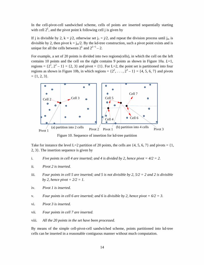
For example, a set of 20 points is divided into two regions(cells), in which the cell on the left contains 10 points and the cell on the right contains 9 points as shown in Figure 10a. L=1, regions = {21, 22 – 1} = {2, 3} and pivot = {1}. For L=2, the point set is partitioned into four regions as shown in Figure 10b, in which regions = {22, . . . , 23 – 1} = {4, 5, 6, 7} and pivots = {1, 2, 3}.

Take for instance the level L=2 partition of 20 points, the cells are {4, 5, 6, 7} and pivots = {1, 2, 3}. The insertion sequence is given by

i. Five points in cell 4 are inserted; and 4 is divided by 2, hence pivot = 4/2 = 2.

ii. Pivot 2 is inserted.

iii. Four points in cell 5 are inserted; and 5 is not divisible by 2, 5/2 = 2 and 2 is divisible by 2, hence pivot = 2/2 = 1.

iv. Pivot 1 is inserted.

v. Four points in cell 6 are inserted; and 6 is divisible by 2, hence pivot = 6/2 = 3.

vi. Pivot 3 is inserted.

vii. Four points in cell 7 are inserted.

viii. All the 20 points in the set have been processed.

By means of the simple cell-pivot-cell sandwiched scheme, points partitioned into kd-tree cells can be inserted in a reasonable contiguous manner without much computation.

Figure 10. Sequence of insertion for kd-tree partition

(a) partition into 2 cells Pivot 1

(b) partition into 4 cells

Cell 2 Cell 3

Cell 4

Cell 5

Cell 6

Cell 7

Pivot 1 Pivot 2 Pivot 3

15

3.4 Enhanced kd-tree insertion

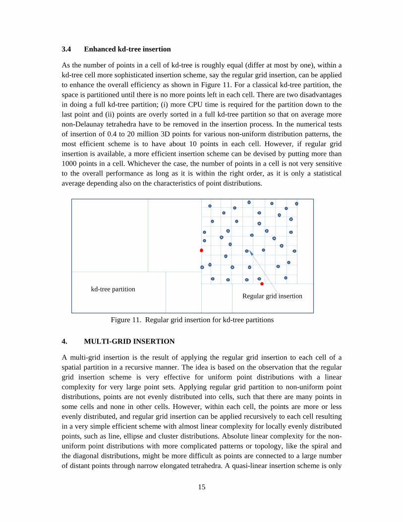
As the number of points in a cell of kd-tree is roughly equal (differ at most by one), within a kd-tree cell more sophisticated insertion scheme, say the regular grid insertion, can be applied to enhance the overall efficiency as shown in Figure 11. For a classical kd-tree partition, the space is partitioned until there is no more points left in each cell. There are two disadvantages in doing a full kd-tree partition; (i) more CPU time is required for the partition down to the last point and (ii) points are overly sorted in a full kd-tree partition so that on average more non-Delaunay tetrahedra have to be removed in the insertion process. In the numerical tests of insertion of 0.4 to 20 million 3D points for various non-uniform distribution patterns, the most efficient scheme is to have about 10 points in each cell. However, if regular grid insertion is available, a more efficient insertion scheme can be devised by putting more than 1000 points in a cell. Whichever the case, the number of points in a cell is not very sensitive to the overall performance as long as it is within the right order, as it is only a statistical average depending also on the characteristics of point distributions.

4. MULTI-GRID INSERTION

A multi-grid insertion is the result of applying the regular grid insertion to each cell of a spatial partition in a recursive manner. The idea is based on the observation that the regular grid insertion scheme is very effective for uniform point distributions with a linear complexity for very large point sets. Applying regular grid partition to non-uniform point distributions, points are not evenly distributed into cells, such that there are many points in some cells and none in other cells. However, within each cell, the points are more or less evenly distributed, and regular grid insertion can be applied recursively to each cell resulting in a very simple efficient scheme with almost linear complexity for locally evenly distributed points, such as line, ellipse and cluster distributions. Absolute linear complexity for the non-uniform point distributions with more complicated patterns or topology, like the spiral and the diagonal distributions, might be more difficult as points are connected to a large number of distant points through narrow elongated tetrahedra. A quasi-linear insertion scheme is only

Figure 11. Regular grid insertion for kd-tree partitions

kd-tree partition Regular grid insertion

16

possible unless the number of tetrahedra removed for each point insertion can be controlled in such a way that it does not increase with the number of points in the set.

4.1 Regular (Uniform) Grid (3D) 4.1.1 Construction of Regular Grid

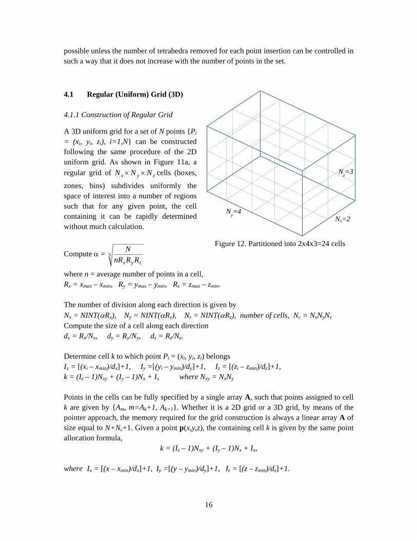
A 3D uniform grid for a set of N points {Pi = (xi, yi, zi), i=1,N} can be constructed following the same procedure of the 2D uniform grid. As shown in Figure 11a, a regular grid of zyx NNN ×× cells (boxes,

zones, bins) subdivides uniformly the space of interest into a number of regions such that for any given point, the cell containing it can be rapidly determined without much calculation.

Compute α = 3zyx RRnR

N

where n = average number of points in a cell, Rx = xmax – xmin, Ry = ymax – ymin, Rz = zmax – zmin. The number of division along each direction is given by Nx = NINT(αRx), Ny = NINT(αRy), Nz = NINT(αRz), number of cells, Nc = NxNyNz Compute the size of a cell along each direction dx = Rx/Nx, dy = Ry/Ny, dz = Rz/Nz. Determine cell k to which point Pi = (xi, yi, zi) belongs Ix = [(xi – xmin)/dx]+1, Iy =[(yi – ymin)/dy]+1, Iz = [(zi – zmin)/dz]+1, k = (Iz – 1)Nxy + (Iy – 1)Nx + Ix where Nxy = NxNy Points in the cells can be fully specified by a single array A, such that points assigned to cell k are given by {Am, m=Ak+1, Ak+1}. Whether it is a 2D grid or a 3D grid, by means of the pointer approach, the memory required for the grid construction is always a linear array A of size equal to N+Nc+1. Given a point p(x,y,z), the containing cell k is given by the same point allocation formula,

k = (Iz – 1)Nxy + (Iy – 1)Nx + Ix, where Ix = [(x – xmin)/dx]+1, Iy =[(y – ymin)/dy]+1, Iz = [(z – zmin)/dz]+1.

Figure 12. Partitioned into 2x4x3=24 cells

Ny=4 Nx=2

Nz=3

17

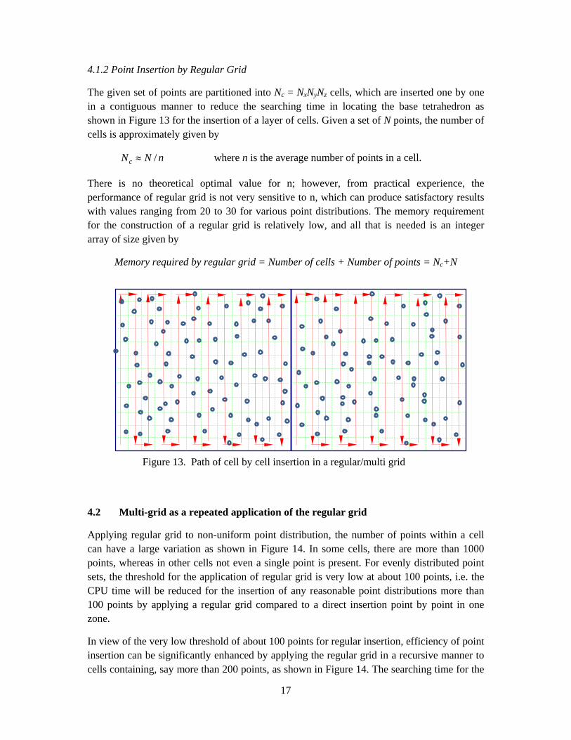
4.1.2 Point Insertion by Regular Grid

The given set of points are partitioned into Nc = NxNyNz cells, which are inserted one by one in a contiguous manner to reduce the searching time in locating the base tetrahedron as shown in Figure 13 for the insertion of a layer of cells. Given a set of N points, the number of cells is approximately given by

nNNc /≈ where n is the average number of points in a cell.

There is no theoretical optimal value for n; however, from practical experience, the performance of regular grid is not very sensitive to n, which can produce satisfactory results with values ranging from 20 to 30 for various point distributions. The memory requirement for the construction of a regular grid is relatively low, and all that is needed is an integer array of size given by

Memory required by regular grid = Number of cells + Number of points = Nc+N

4.2 Multi-grid as a repeated application of the regular grid

Applying regular grid to non-uniform point distribution, the number of points within a cell can have a large variation as shown in Figure 14. In some cells, there are more than 1000 points, whereas in other cells not even a single point is present. For evenly distributed point sets, the threshold for the application of regular grid is very low at about 100 points, i.e. the CPU time will be reduced for the insertion of any reasonable point distributions more than 100 points by applying a regular grid compared to a direct insertion point by point in one zone.

In view of the very low threshold of about 100 points for regular insertion, efficiency of point insertion can be significantly enhanced by applying the regular grid in a recursive manner to cells containing, say more than 200 points, as shown in Figure 14. The searching time for the

Figure 13. Path of cell by cell insertion in a regular/multi grid

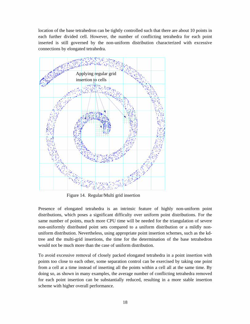
18

location of the base tetrahedron can be tightly controlled such that there are about 10 points in each further divided cell. However, the number of conflicting tetrahedra for each point inserted is still governed by the non-uniform distribution characterized with excessive connections by elongated tetrahedra.

Presence of elongated tetrahedra is an intrinsic feature of highly non-uniform point distributions, which poses a significant difficulty over uniform point distributions. For the same number of points, much more CPU time will be needed for the triangulation of severe non-uniformly distributed point sets compared to a uniform distribution or a mildly non-uniform distribution. Nevertheless, using appropriate point insertion schemes, such as the kd-tree and the multi-grid insertions, the time for the determination of the base tetrahedron would not be much more than the case of uniform distribution.

To avoid excessive removal of closely packed elongated tetrahedra in a point insertion with points too close to each other, some separation control can be exercised by taking one point from a cell at a time instead of inserting all the points within a cell all at the same time. By doing so, as shown in many examples, the average number of conflicting tetrahedra removed for each point insertion can be substantially reduced, resulting in a more stable insertion scheme with higher overall performance.

Figure 14. Regular/Multi grid insertion

Applying regular grid insertion to cells

19

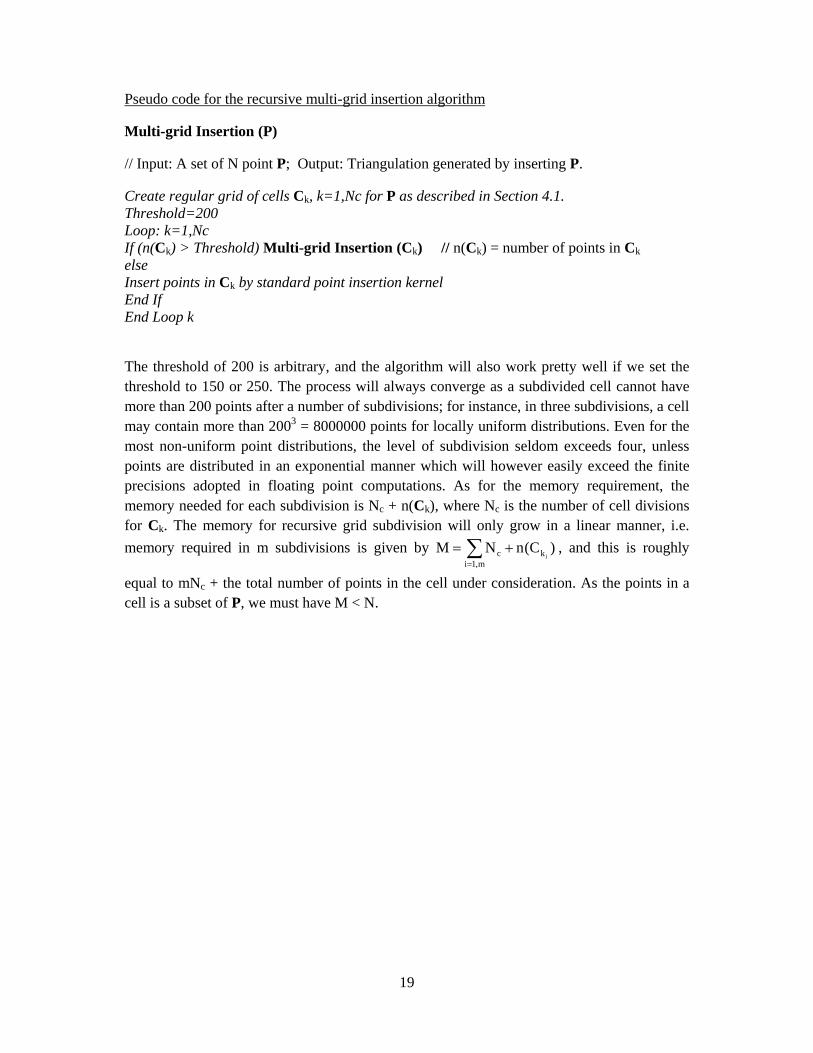
Pseudo code for the recursive multi-grid insertion algorithm

Multi-grid Insertion (P)

// Input: A set of N point P; Output: Triangulation generated by inserting P.

Create regular grid of cells Ck, k=1,Nc for P as described in Section 4.1. Threshold=200 Loop: k=1,Nc If (n(Ck) > Threshold) Multi-grid Insertion (Ck) // n(Ck) = number of points in Ck else Insert points in Ck by standard point insertion kernel End If End Loop k

The threshold of 200 is arbitrary, and the algorithm will also work pretty well if we set the threshold to 150 or 250. The process will always converge as a subdivided cell cannot have more than 200 points after a number of subdivisions; for instance, in three subdivisions, a cell may contain more than 2003 = 8000000 points for locally uniform distributions. Even for the most non-uniform point distributions, the level of subdivision seldom exceeds four, unless points are distributed in an exponential manner which will however easily exceed the finite precisions adopted in floating point computations. As for the memory requirement, the memory needed for each subdivision is Nc + n(Ck), where Nc is the number of cell divisions for Ck. The memory for recursive grid subdivision will only grow in a linear manner, i.e. memory required in m subdivisions is given by ∑

=

+=m,1i

kc )C(nNMi

, and this is roughly

equal to mNc + the total number of points in the cell under consideration. As the points in a cell is a subset of P, we must have M < N.

20

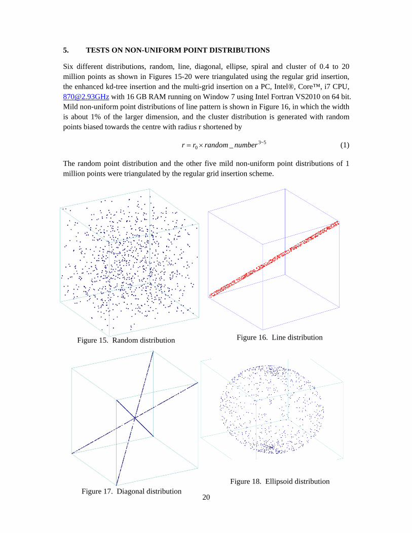
5. TESTS ON NON-UNIFORM POINT DISTRIBUTIONS

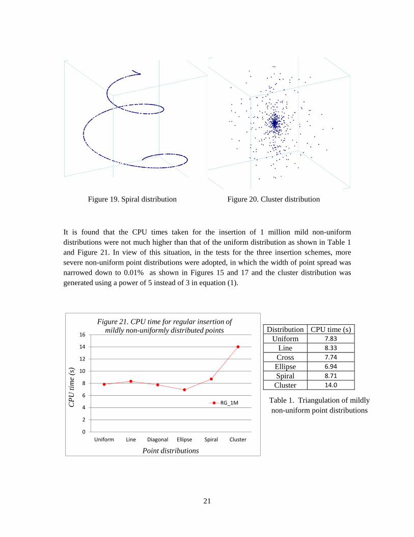
Six different distributions, random, line, diagonal, ellipse, spiral and cluster of 0.4 to 20 million points as shown in Figures 15-20 were triangulated using the regular grid insertion, the enhanced kd-tree insertion and the multi-grid insertion on a PC, Intel®, Core™, i7 CPU, 870@2.93GHz with 16 GB RAM running on Window 7 using Intel Fortran VS2010 on 64 bit. Mild non-uniform point distributions of line pattern is shown in Figure 16, in which the width is about 1% of the larger dimension, and the cluster distribution is generated with random points biased towards the centre with radius r shortened by

5~30 _ numberrandomrr ×= (1)

The random point distribution and the other five mild non-uniform point distributions of 1 million points were triangulated by the regular grid insertion scheme.

Figure 15. Random distribution Figure 16. Line distribution

Figure 17. Diagonal distribution Figure 18. Ellipsoid distribution

21

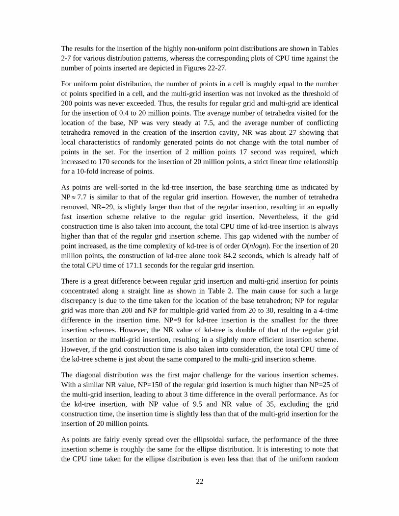
It is found that the CPU times taken for the insertion of 1 million mild non-uniform distributions were not much higher than that of the uniform distribution as shown in Table 1 and Figure 21. In view of this situation, in the tests for the three insertion schemes, more severe non-uniform point distributions were adopted, in which the width of point spread was narrowed down to 0.01% as shown in Figures 15 and 17 and the cluster distribution was generated using a power of 5 instead of 3 in equation (1).

0

2

4

6

8

10

12

14

16

Uniform Line Diagonal Ellipse Spiral Cluster

CPU

tim

e (s

)

Point distributions

Figure 21. CPU time for regular insertion of mildly non-uniformly distributed points

RG_1M

Distribution CPU time (s)Uniform 7.83 

Line 8.33 Cross 7.74 Ellipse 6.94 Spiral 8.71 Cluster 14.0 

Figure 19. Spiral distribution Figure 20. Cluster distribution

Table 1. Triangulation of mildly non-uniform point distributions

22

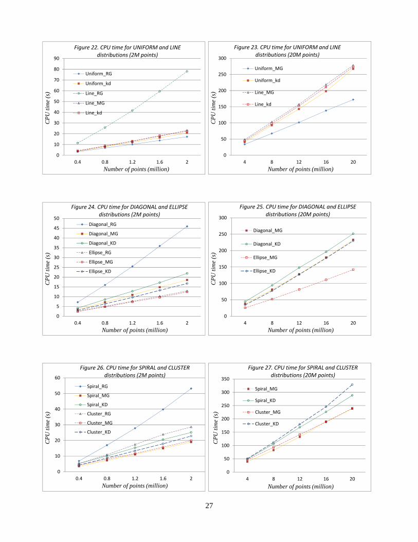
The results for the insertion of the highly non-uniform point distributions are shown in Tables 2-7 for various distribution patterns, whereas the corresponding plots of CPU time against the number of points inserted are depicted in Figures 22-27.

For uniform point distribution, the number of points in a cell is roughly equal to the number of points specified in a cell, and the multi-grid insertion was not invoked as the threshold of 200 points was never exceeded. Thus, the results for regular grid and multi-grid are identical for the insertion of 0.4 to 20 million points. The average number of tetrahedra visited for the location of the base, NP was very steady at 7.5, and the average number of conflicting tetrahedra removed in the creation of the insertion cavity, NR was about 27 showing that local characteristics of randomly generated points do not change with the total number of points in the set. For the insertion of 2 million points 17 second was required, which increased to 170 seconds for the insertion of 20 million points, a strict linear time relationship for a 10-fold increase of points.

As points are well-sorted in the kd-tree insertion, the base searching time as indicated by NP 7.7≈ is similar to that of the regular grid insertion. However, the number of tetrahedra removed, NR=29, is slightly larger than that of the regular insertion, resulting in an equally fast insertion scheme relative to the regular grid insertion. Nevertheless, if the grid construction time is also taken into account, the total CPU time of kd-tree insertion is always higher than that of the regular grid insertion scheme. This gap widened with the number of point increased, as the time complexity of kd-tree is of order O(nlogn). For the insertion of 20 million points, the construction of kd-tree alone took 84.2 seconds, which is already half of the total CPU time of 171.1 seconds for the regular grid insertion.

There is a great difference between regular grid insertion and multi-grid insertion for points concentrated along a straight line as shown in Table 2. The main cause for such a large discrepancy is due to the time taken for the location of the base tetrahedron; NP for regular grid was more than 200 and NP for multiple-grid varied from 20 to 30, resulting in a 4-time difference in the insertion time. NP=9 for kd-tree insertion is the smallest for the three insertion schemes. However, the NR value of kd-tree is double of that of the regular grid insertion or the multi-grid insertion, resulting in a slightly more efficient insertion scheme. However, if the grid construction time is also taken into consideration, the total CPU time of the kd-tree scheme is just about the same compared to the multi-grid insertion scheme.

The diagonal distribution was the first major challenge for the various insertion schemes. With a similar NR value, NP=150 of the regular grid insertion is much higher than NP=25 of the multi-grid insertion, leading to about 3 time difference in the overall performance. As for the kd-tree insertion, with NP value of 9.5 and NR value of 35, excluding the grid construction time, the insertion time is slightly less than that of the multi-grid insertion for the insertion of 20 million points.

As points are fairly evenly spread over the ellipsoidal surface, the performance of the three insertion scheme is roughly the same for the ellipse distribution. It is interesting to note that the CPU time taken for the ellipse distribution is even less than that of the uniform random

23

distribution for the insertion of 0.4 to 20 million points. A possible cause for this to happen is that may be the average number of points in a cell for the ellipse distribution is closer to the optimal number of insertion (20 – 30) compared to the case of uniform distribution, in which the specified number of points in a cell had been set equal to 8.

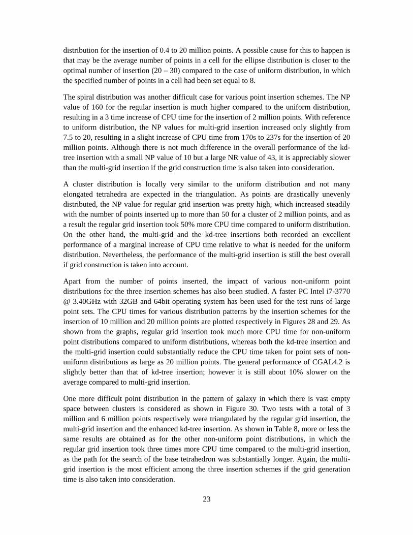
The spiral distribution was another difficult case for various point insertion schemes. The NP value of 160 for the regular insertion is much higher compared to the uniform distribution, resulting in a 3 time increase of CPU time for the insertion of 2 million points. With reference to uniform distribution, the NP values for multi-grid insertion increased only slightly from 7.5 to 20, resulting in a slight increase of CPU time from 170s to 237s for the insertion of 20 million points. Although there is not much difference in the overall performance of the kd-tree insertion with a small NP value of 10 but a large NR value of 43, it is appreciably slower than the multi-grid insertion if the grid construction time is also taken into consideration.

A cluster distribution is locally very similar to the uniform distribution and not many elongated tetrahedra are expected in the triangulation. As points are drastically unevenly distributed, the NP value for regular grid insertion was pretty high, which increased steadily with the number of points inserted up to more than 50 for a cluster of 2 million points, and as a result the regular grid insertion took 50% more CPU time compared to uniform distribution. On the other hand, the multi-grid and the kd-tree insertions both recorded an excellent performance of a marginal increase of CPU time relative to what is needed for the uniform distribution. Nevertheless, the performance of the multi-grid insertion is still the best overall if grid construction is taken into account.

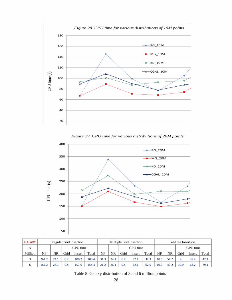
Apart from the number of points inserted, the impact of various non-uniform point distributions for the three insertion schemes has also been studied. A faster PC Intel i7-3770 @ 3.40GHz with 32GB and 64bit operating system has been used for the test runs of large point sets. The CPU times for various distribution patterns by the insertion schemes for the insertion of 10 million and 20 million points are plotted respectively in Figures 28 and 29. As shown from the graphs, regular grid insertion took much more CPU time for non-uniform point distributions compared to uniform distributions, whereas both the kd-tree insertion and the multi-grid insertion could substantially reduce the CPU time taken for point sets of non-uniform distributions as large as 20 million points. The general performance of CGAL4.2 is slightly better than that of kd-tree insertion; however it is still about 10% slower on the average compared to multi-grid insertion.

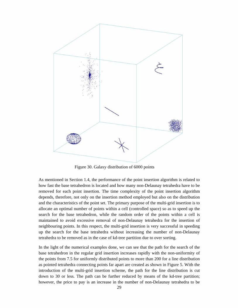
One more difficult point distribution in the pattern of galaxy in which there is vast empty space between clusters is considered as shown in Figure 30. Two tests with a total of 3 million and 6 million points respectively were triangulated by the regular grid insertion, the multi-grid insertion and the enhanced kd-tree insertion. As shown in Table 8, more or less the same results are obtained as for the other non-uniform point distributions, in which the regular grid insertion took three times more CPU time compared to the multi-grid insertion, as the path for the search of the base tetrahedron was substantially longer. Again, the multi-grid insertion is the most efficient among the three insertion schemes if the grid generation time is also taken into consideration.

24

UNIFORM  Regular Grid Insertion  Multiple Grid Insertion  kd‐tree Insertion N CPU time CPU time CPU time

(Million) NP NR Grid Insert Total NP NR Grid Insert Total NP NR Grid Insert Total 0.4  7.4  26.4  0.04  3.28  3.32  7.4  26.4 0.04  3.28  3.32  7.92 28.5 0.485  3.23  3.715 0.8  7.54  26.9  0.08  6.69  6.77  7.54 26.9 0.08  6.69  6.77  7.53 28.8 1.35  6.59  7.94 1.2  7.57  27.2  0.12  9.99  10.11  7.57 27.2 0.12  9.99  10.11  7.73 29.1 2.2  9.82  12.02 1.6 7.63  27.3  0.17  13.6  13.77  7.63 27.3 0.17  13.6  13.77  8.09 29.4 3.14  13.2  16.34 2  7.64  27.5  0.22  17  17.22  7.64 27.5 0.22  17  17.22  7.53 28.9 4.21  16.6  20.81 4            8.63 26.5 0.37  33.4  33.77  7.23 28.8 9.55  31  40.55 8            8.66 26.9 0.76  66.5  67.26  7.64 29.3 23.4  69.2  92.6 12           8.74 27.1 1.26  100.2  101.46  8.1  29.8 40.6  102.4  143 16            8.75 27.3 1.85  136.3  138.15  7.62 29.3 62.5  135.5  198 20            8.78 27.4 2.39  169.7  172.09  7.86 29.5 84.2  183.1  267.3 

LINE  Regular Grid Insertion  Multiple Grid Insertion  kd‐tree Insertion N CPU time CPU time CPU time

(Million) NP NR Grid Insert Total NP NR Grid Insert Total NP NR Grid Insert Total 0.4  211.7  18.8  0.03  11.3  11.33  30.6 18.8 0.03  3.85  3.88  8.91  38.2  0.36  3.89  4.25 0.8  226.7  19  0.06  25.7  25.76  28.9 19  0.06  8.3  8.36  9.06  38.3  0.92  7.75  8.67 1.2  231.9  19.1  0.08  41.5  41.58  26.8 19.1 0.08  12.9  12.98  8.72  38  1.58  11.6  13.18 1.6 237.1  19.2  0.1  59.3  59.4  25.3 19.2 0.1  17.7  17.8  9.06  38.4  2.35  15.9  18.25 2  238.4  19.3  0.12  77.9  78.02  25.1 19.3 0.12  23  23.12  8.5  37.9  3.16  19.3  22.46 4            23.5 19.4 0.26  48.2  48.46  8.51  38.1  7.32  37.5  44.82 8            22.6 19.6 0.49  102.5  102.99  9.44  38.4  18.5  79  97.5 12           21.5 19.6 0.76  156.6  157.36  9.01  38.6  32.5  120.1  152.6 16            21.6 19.7 1.03  217.6  218.63  9.46  38.5  46.5  164.6  211.1 20            21.2 19.7 1.28  277.2  278.48  9.37  38.7  66  207.5  273.5 

Table 2. Uniform distribution

Table 3. Line distribution

25

DIAGONAL  Regular Grid Insertion  Multiple Grid Insertion  kd‐tree Insertion N CPU time CPU time CPU time

(Million) NP NR Grid Insert Total NP NR Grid Insert Total NP NR Grid Insert Total 0.4  130.4  18.5  0.03  7.12  7.15  28.7 18.5 0.03  3.45  3.48  9.43  35.5  0.36  3.75  4.11 0.8  144.9  19  0.05  15.9  15.95  27.3 19  0.05  7.11  7.16  9.79  35.2  0.89  7.65  8.54 1.2  150.4  19.1  0.08  25.4  25.48  25.3 19.1 0.08  10.8  10.88  9.6  35.8  1.47  11.3  12.77 1.6 155  19.3  0.1  35.8  35.9  25.3 19.3 0.1  14.7  14.8  9.5  35.4  2.25  14.9  17.15 2  156.8  19.3  0.13  45.8  45.93  23.5 19.3 0.13  18.4  18.53  9.16  35  3.12  18.8  21.92 4            21.9 19.5 0.27  37.2  37.47  9.15  35.1  8.05  36.4  44.45 8            20.8 19.7 0.49  80.5  80.99  8.77  35.2  18.8  75.2  94 12           20.4 19.8 0.76  127.2  127.96  9.36  35.5  32.6  115.3  147.9 16            20  19.9 1.03  178  179.03  8.71  35.2  45.9  150.3  196.2 20            21.3 19.9 1.3  231.7  233  8.94  35.5  60.8  190.6  251.4 

ELLIPSE  Regular Grid Insertion  Multiple Grid Insertion  kd‐tree Insertion N CPU time CPU time CPU time

(Million) NP NR Grid Insert Total NP NR Grid Insert Total NP NR Grid Insert Total 0.4  12.6  17.7  0.03  2.56  2.59  9.81 17.7 0.03 2.38  2.41  6.93  23.3  0.48  2.55  3.03 0.8  13.4  17.2  0.06  5  5.06  9.66 17.2 0.06 4.76  4.82  6.97  23.1  1.19  5.14  6.33 1.2  13.8  17.2  0.08  7.61  7.69  9.41 17.2 0.08 7.26  7.34  6.81  23.1  2.09  7.53  9.62 1.6 14.4  17.2  0.1  10.1  10.2  9.3  17.2 0.1  9.55  9.65  7.06  23.6  2.93  10.3  13.23 2  14.7  17.3  0.12  12.8  12.92  9.24 17.3 0.12 12.3  12.42  6.82  23.5  3.94  12.8  16.74 4            9.33 18  0.26 25.2  25.46  6.98  24.5  8.91  25.4  34.31 8            9.69 18.8 0.48 51.7  52.18  7.21  25.7  23.4  54  77.4 12           9.92 19.2 0.76 80.5  81.26  7.64  26.7  39.1  88  127.1 16            10.1 19.5 1.03 109.9  110.93  7.44  26.9  58.9  118.3  177.2 20            10.2 19.8 1.29 140.8  142.09  7.66  27.4  79.3  150.6  229.9 

Table 4. Diagonal distribution

Table 5. Ellipse distribution

26

SPIRAL  Regular Grid Insertion  Multiple Grid Insertion  kd‐tree Insertion N CPU time CPU time CPU time

(Million) NP NR Grid Insert Total NP NR Grid Insert Total NP NR Grid Insert Total 0.4  109.3  22.6  0.03 6.82  6.85  18.8 22.6 0.03 3.43  3.46  10.1  48.3  0.38  4.8  5.18 0.8  141.4  21.6  0.05 16.9  16.95  20  21.6 0.05 7.15  7.2  10.2  44.8  0.98  9.12  10.1 1.2  157.3  21.4  0.08 27.7  27.78  20.4 21.4 0.08 11  11.08  10  43.2  1.7  13.6  15.3 1.6 167.8  21  0.1  39.7  39.8  20.7 21  0.1  14.8  14.9  10.2  42.4  2.53  18  20.53 2  177.3  20.9  0.13 53  53.13  20.9 20.9 0.13 18.8  18.93  10.1  41.5  3.43  21.7  25.13 4            21  20.5 0.26 39  39.26  9.74  40.5  7.93  41.4  49.33 8            21.5 20.4 0.48 82  82.48  9.5  39.5  19.9  86.2  106.1 12           22.2 20.3 0.76 131.8  132.56  9.98  39.2  35.7  132.7  168.4 16            21.7 20.3 1.03 188.1  189.13  9.55  38.9  52.8  173.4  226.2 20            22.2 20.3 1.29 236.7  237.99  9.61  38.8  70.9  217.5  288.4 

CLUSTER  Regular Grid Insertion  Multiple Grid Insertion  kd‐tree Insertion N CPU time CPU time CPU time

(Million) NP NR Grid Insert Total NP NR Grid Insert Total NP NR Grid Insert Total 0.4  43  23.4  0.03  5.25  5.28  14.5 23.4 0.03 4.06  4.09  11.4  33  0.46  3.77  4.23 0.8  43.8  24  0.05  10.8  10.85  14.3 24  0.05 7.99  8.04  12.1  33.5  1.15  7.59  8.74 1.2  53  23.9  0.08  17.3  17.38  14.3 23.9 0.08 11.5  11.58  12.2  33.7  1.93  11.4  13.33 1.6 53.3  24  0.11  23.7  23.81  14.8 24  0.11 15.6  15.71  12.8  34  2.65  15.2  17.85 2  50.1  24.4  0.13  28.5  28.63  14.8 24.4 0.13 19.8  19.93  13  34.2  3.6  19.2  22.8 4            15.1 24.5 0.27 46.7  46.97  14.4  34.7  9.24  41.2  50.44 8            15.4 24.8 0.49 92.5  92.99  16.1  35.3  22.8  89.1  111.9 12           15.4 24.9 0.76 140.3  141.06  17.8  35.7  39.8  140  179.8 16            15.5 25.1 1.03 187.8  188.83  18.5  35.9  58.5  187.2  245.7 20            15.4 25.2 1.3  238.5  239.8  19.3  36  78.9  250  328.9 

Table 6. Spiral distribution

Table 7. Cluster distribution

27

0

10

20

30

40

50

60

70

80

90

0.4 0.8 1.2 1.6 2

CPU

tim

e (s

)

Number of points (million)

Figure 22. CPU time for UNIFORM and LINE distributions (2M points)

Uniform_RG

Uniform_kd

Line_RG

Line_MG

Line_kd

0

50

100

150

200

250

300

4 8 12 16 20

CPU

tim

e (s

)

Number of points (million)

Figure 23. CPU time for UNIFORM and LINE distributions (20M points)

Uniform_MG

Uniform_kd

Line_MG

Line_kd

0

5

10

15

20

25

30

35

40

45

50

0.4 0.8 1.2 1.6 2

CPU

tim

e (s

)

Number of points (million)

Figure 24. CPU time for DIAGONAL and ELLIPSE distributions (2M points)

Diagonal_RG

Diagonal_MG

Diagonal_KD

Ellipse_RG

Ellipse_MG

Ellipse_KD

0

50

100

150

200

250

300

4 8 12 16 20

CPU

tim

e (s

)

Number of points (million)

Figure 25. CPU time for DIAGONAL and ELLIPSE distributions (20M points)

Diagonal_MG

Diagonal_KD

Ellipse_MG

Ellipse_KD

0

10

20

30

40

50

60

0.4 0.8 1.2 1.6 2

CPU

tim

e (s

)

Number of points (million)

Figure 26. CPU time for SPIRAL and CLUSTER distributions (2M points)

Spiral_RG

Spiral_MG

Spiral_KD

Cluster_RG

Cluster_MG

Cluster_KD

0

50

100

150

200

250

300

350

4 8 12 16 20

CPU

tim

e (s

)

Number of points (million)

Figure 27. CPU time for SPIRAL and CLUSTER distributions (20M points)

Spiral_MG

Spiral_KD

Cluster_MG

Cluster_KD

28

20

40

60

80

100

120

140

160

180

CPU

time (

s)

Figure 28. CPU time for various distributions of 10M points

RG_10M

MG_10M

KD_10M

CGAL_10M

50

100

150

200

250

300

350

400

CPU

time (

s)

Figure 29. CPU time for various distributions of 20M points

RG_20M

MG_20M

KD_20M

CGAL_20M

GALAXY  Regular Grid Insertion  Multiple Grid Insertion  kd‐tree Insertion 

N CPU time CPU time CPU time Million NP NR Grid Insert Total NP NR Grid Insert Total NP NR Grid Insert Total

3  261.2  24.1  0.2  100.2  100.4  31.3  24.1  0.2  32.1  32.3  10.5  54.7  4  38.4  42.4 

6  167.2  26.1  0.4  153.9  154.3  21.2  26.1  0.4  62.1  62.5  10.3  43.2  10.9  68.2  79.1 

Table 8. Galaxy distribution of 3 and 6 million points

29

As mentioned in Section 1.4, the performance of the point insertion algorithm is related to how fast the base tetrahedron is located and how many non-Delaunay tetrahedra have to be removed for each point insertion. The time complexity of the point insertion algorithm depends, therefore, not only on the insertion method employed but also on the distribution and the characteristics of the point set. The primary purpose of the multi-grid insertion is to allocate an optimal number of points within a cell (controlled space) so as to speed up the search for the base tetrahedron, while the random order of the points within a cell is maintained to avoid excessive removal of non-Delaunay tetrahedra for the insertion of neighbouring points. In this respect, the multi-grid insertion is very successful in speeding up the search for the base tetrahedra without increasing the number of non-Delaunay tetrahedra to be removed as in the case of kd-tree partition due to over sorting.

In the light of the numerical examples done, we can see that the path for the search of the base tetrahedron in the regular grid insertion increases rapidly with the non-uniformity of the points from 7.5 for uniformly distributed points to more than 200 for a line distribution as pointed tetrahedra connecting points far apart are created as shown in Figure 5. With the introduction of the multi-grid insertion scheme, the path for the line distribution is cut down to 30 or less. The path can be further reduced by means of the kd-tree partition; however, the price to pay is an increase in the number of non-Delaunay tetrahedra to be

Figure 30. Galaxy distribution of 6000 points

30

removed for each point insertion as points are so close to each other in a kd-tree partition, resulting in a more or less equally efficient insertion scheme without counting the grid construction time. It is an open question whether we could reduce the path to the level of that of the kd-tree without increasing the non-Delaunay tetrahedra to be removed for each point insertion. Nevertheless, the spiral and the galaxy point distributions may be among the worst cases as tetrahedra are connected to boundary points; but then even in these difficult cases, the CPU time needed is less than twice for that of a uniform point distribution by the multi-grid insertion algorithm.

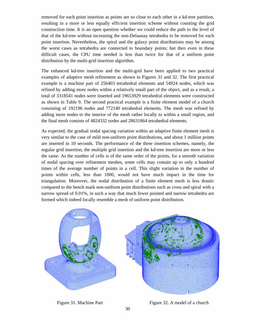
The enhanced kd-tree insertion and the multi-grid have been applied to two practical examples of adaptive mesh refinement as shown in Figures 31 and 32. The first practical example is a machine part of 256403 tetrahedral elements and 54924 nodes, which was refined by adding more nodes within a relatively small part of the object, and as a result, a total of 3318541 nodes were inserted and 19653929 tetrahedral elements were constructed as shown in Table 9. The second practical example is a finite element model of a church consisting of 192196 nodes and 772140 tetrahedral elements. The mesh was refined by adding more nodes to the interior of the mesh rather locally to within a small region, and the final mesh consists of 4824332 nodes and 28631864 tetrahedral elements.

As expected, the gradual nodal spacing variation within an adaptive finite element mesh is very similar to the case of mild non-uniform point distributions, and about 1 million points are inserted in 10 seconds. The performance of the three insertion schemes, namely, the regular grid insertion, the multiple grid insertion and the kd-tree insertion are more or less the same. As the number of cells is of the same order of the points, for a smooth variation of nodal spacing over refinement meshes, some cells may contain up to only a hundred times of the average number of points in a cell. This slight variation in the number of points within cells, less than 1000, would not have much impact in the time for triangulation. Moreover, the nodal distribution of a finite element mesh is less drastic compared to the bench mark non-uniform point distributions such as cross and spiral with a narrow spread of 0.01%, in such a way that much fewer pointed and narrow tetrahedra are formed which indeed locally resemble a mesh of uniform point distribution.

Figure 31. Machine Part Figure 32. A model of a church

31

Regular Grid Insertion Multiple Grid Insertion kd-tree Insertion CPU time CPU time CPU time NP NR Grid Insert Total NP NR Grid Insert Total NP NR Grid Insert Total

Machine 7.92  38.2  0.21  32.97  33.18  7.34  38.2  0.21  29.21  29.42  17.4  31.0  3.9  29.2  33.1 

Church 8.35  34.1  0.29  44.2  44.49  7.66  34.1  0.29  42.1  42.39  39.2  38.0  4.74  61.3  65.04 

6 POSSIBILITY FOR PARALLELIZATION

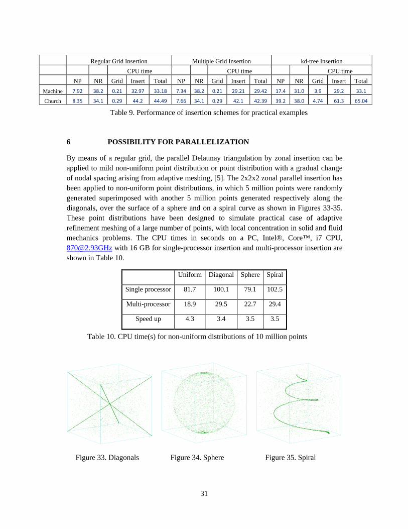
By means of a regular grid, the parallel Delaunay triangulation by zonal insertion can be applied to mild non-uniform point distribution or point distribution with a gradual change of nodal spacing arising from adaptive meshing, [5]. The 2x2x2 zonal parallel insertion has been applied to non-uniform point distributions, in which 5 million points were randomly generated superimposed with another 5 million points generated respectively along the diagonals, over the surface of a sphere and on a spiral curve as shown in Figures 33-35. These point distributions have been designed to simulate practical case of adaptive refinement meshing of a large number of points, with local concentration in solid and fluid mechanics problems. The CPU times in seconds on a PC, Intel®, Core™, i7 CPU, 870@2.93GHz with 16 GB for single-processor insertion and multi-processor insertion are shown in Table 10.

Uniform Diagonal Sphere Spiral

Single processor 81.7 100.1 79.1 102.5

Multi-processor 18.9 29.5 22.7 29.4

Speed up 4.3 3.4 3.5 3.5

Table 9. Performance of insertion schemes for practical examples

Table 10. CPU time(s) for non-uniform distributions of 10 million points

Figure 33. Diagonals Figure 34. Sphere Figure 35. Spiral

32

For highly non-uniform point distributions with point concentration within a region of 0.01% of the larger dimension, the multi-grid insertion could be applied. As the multi-grid is a just regular grid on top of another regular grid, the parallel insertion designed for regular grid can also be applied to multi-grid insertion. However, it is more difficult for the parallelization of kd-tree insertion, as the cells of a kd-tree partition is not in alignment going from one cell to the adjacent cells.

7 CONCLUSIONS AND DISCUSSIONS

The fundamentals for the Delaunay triangulations of non-uniformly distributed points by the insertion method are discussed. In the light of the simplicity and linearity of regular grid insertion, a multi-grid insertion scheme is proposed for the triangulation of uniform and non-uniform point distributions by recursive application of the regular grid insertion to an arbitrary subset of the original point set.

The performance of all the insertion schemes, namely, the regular grid, the multi-grid and the enhanced kd-tree is quite promising, in which only the regular grid insertion showed a poor performance for the line and the spiral distributions. The regular grid insertion is very sensitive to point distribution concentrated along a curve or towards a point, as the time taken in searching for the base tetrahedron increases rapidly with highly non-uniformly distributed points.

Excellent performance of the multi-grid and the enhanced kd-tree insertions is observed for large highly non-uniformly distributed point sets, such that the CPU time taken is no more than double of that of a uniform distribution for the insertion of 20 million points. Compared to the multi-grid insertion, the NP value of kd-tree insertion is usually smaller but this is often offset by a larger NR value for triangulations characterized with a large amount of elongated tetrahedra, resulting in a similar overall performance for the two schemes.

The multi-grid insertion is the most efficient and stable for all the distribution patterns tested among the three insertion schemes if the grid construction time is also taken into account. A quasi-linear complexity can be observed for the triangulation of distribution patterns with local features similar to those of a uniform point distribution, such as line, ellipse and cluster, etc. However, a bit more CPU time is needed for the triangulation of more difficult distribution patterns, such as diagonal and spiral, in which there are many elongated tetrahedra in the triangulation leading to a slightly nonlinear complexity. Nevertheless, with the multi-grid insertion, the triangulation time of the worst non-uniform distribution of 20 million points tested is about only 60% more than that of a uniform distribution, which is already a couple of times faster than existing triangulation schemes.

33

ACKNOWLEDGEMENTS

The financial support from the HKSAR GRF Grant to the research project HKU715110E on “Drifted based seismic fragility analysis of high-rise RC buildings with transfer structures” is greatly acknowledged.

REFERENCES

[1] Hans Meine, Ullrich Kothe, Peer Stelldinger, “A topological sampling theorem for robust boundary reconstruction and image segmentation”, Discrete Applied Mathematics, 157 (2009) 524-541

[2] H. Borouchaki and S.H. Lo, “Fast Delaunay triangulation in three dimensions”, Comput. Methods Appl. Mech. Engrg. 128 (1995) 153-167

[3] Peter Su and Robert L. Scot Drysdale, “A comparison of sequential Delaunay triangulation algorithms”, Computational Geometry, 7 (1997) 361-385

[4] S.H. Lo, “Parallel Delaunay triangulation – Application to two dimensions”, Finite Elements in Analysis and Design, 62 (2012) 37-48

[5] S.H. Lo, “Parallel Delaunay Triangulation in three dimensions”, Comput. Methods Appl. Mech. Engrg., 237 (2012) 88-106

[6] B. Delaunay, “Sur la sphere vide”, Bull. Acad. Sci. URSS, Class. Sc. Nat., 793-800, 193

[7] Amenta, N., Choi, S., Rote, G., Incremental constructions con BRIO. In: Proc. 19th Annu. ACM Sympos. Comput. Geom., pp. 211–219. ACM Press, New York (2003)

[8] Liu, Y., Snoeyink, J., A comparison of five implementations of 3d Delaunay tesselation. In: Goodman, J.E., Pach, J., Welzl, E. (eds.) Combinatorial and Computational Geometry. MSRI Publications, vol. 52, pp. 439–458. Cambridge University (2005)

[9] Zhou, S., Jones, C.B., HCPO: An efficient insertion order for incremental Delaunay triangulation, Inf. Process. Lett. 93(1), 37–42 (2005)

[10] J.D. Boissonnat, O. Devillers, S. Hornus, “Incremental construction of the Delaunay triangulation and the Delaunay graph in medium dimension”, 25th Annual Symposium on Computational Geometry, Aarhus, Denmark, 8-10 June 2009

[11] Buchin, K., Organizing Point Sets: Space-Filling Curves, Delaunay Tessellations of Random Point Sets, and Flow Complexes, PhD thesis, Free University Berlin (2007).

[12] Buchin, K. Constructing Delaunay triangulations along space-filling curves. In Proc. 2nd Internat. Sympos. Voronoi Diagrams in Science and Engineering, pages 184--195, Seoul, Korea, 2005.

[13] Kun Zhou, Minmin Gong, Xin Huang, Baining Guo, “Data-parallel Octree for surface reconstruction”, IEEE Transactions on Visualization and Computer Graphics, Vol. 17, No. 5, May 2011, 669-681

[14] Kun Zhou, Minmin Gong, Xin Huang, Baining Guo, “Data-parallel Octree for surface reconstruction”, IEEE Transactions on Visualization and Computer Graphics, Vol. 17, No. 5, May 2011, 669-681

[15] Lemaire C and Moreau JM (2000), “A probabilistic result on multi-dimensional Delaunay triangulations, and its application to the 2D case”, Computational Geometry, 17, 69-96

34

[16] B. Joe, Construction of three-dimensional Delaunay triangulations using local transformations, Computer Aided Geometric Design, 10(4), 123-142, 1989.

[17] H. Edelsbrunner and N. R. Shah, Incremental topological flipping works for regular triangulations. Algorithmica, 15:223–241, 1996.

[18] http://cm.bell-labs.com/netlib/voronoi/hull.html

[19] ftp://ftp.ncsa.uiuc.edu/Visualization/Alpha-shape/

[20] J.D. Boissonnat, O. Devillers, S. Pion, M. Teillaud, M. Yvinec, “Triangulation in CGAL”, Computational Geometry, 22, Issue 1-3, May 2002, 5-19

[21] G. Peano, Sur une courbe, qui remplit toute une aire plane, Mathematische Annalen 36 (1890) 157–160.

[22] D. Hilbert, Über die stetige Abbildung einer Linie auf ein Flächenstück, Mathematische Annalen 38 (1891), 459–460.

[23] Jianfei Liu, Jinhui Yan, S.H. Lo, “A new insertion sequence for incremental Delaunay triangulation”, ACTA Mechanica Sinica, 29, Issue 1 (Feb. 2013) 99-109

[24] Devroye L, Jabbour J, Zamora-Cura C (2000), “Squarish k-d trees”, SIAM Journal of Computing, 30, Issue 5, 1678-1700

[25] Devroye L, Lemaire C, Moreau JM (2004), “Expected time analysis for Delaunay point location”, Computational Geometry, 29, 61-89

[26] Baker TJ (1992) "Tetrahedral mesh generation by a constrained Delaunay triangulation", E.N. Houtis and J.R. Rice eds., Artificial Intelligence, Expert System and Symbolic Computing (Elsevier Science Publishers, B.V., North –Holland, 1992)

[27] Shewchuk JR (1997) "Adaptive precision floating-point arithmetic and fast robust geometric predicates", Discrete Comput. Geom., 18, 305-363.

[28] Devillers O and Preparata FP (1999) Further results on arithmetic filters for geometric predicates, Computational Geometry, 13, 141-148.

[29] Goliaz NA and Dutton RW (1997) Delaunay triangulation and 3D adaptive mesh generation, Finite Elements in Analysis and Design, 25, Issue 3-4, 331-341.