Time Series Forecasting

0Mu Sigma Confidential

Chicago, IL

Bangalore, India

www.mu-sigma.com

Proprietary Information

"This document and its attachments are confidential. Anyunauthorized copying, disclosure or distribution of the material is strictly forbidden"

Chicago, IL

Bangalore, India

www.mu-sigma.com

Proprietary Information

"This document and its attachments are confidential. Anyunauthorized copying, disclosure or distribution of the material is strictly forbidden"

Do The Math

Time Series Forecasting

April 2019

1Mu Sigma ConfidentialTIME SERIES MODELING


Tim

e S

eri

es M

od

elin

g

Time Series Basics

Basic Time Series Modeling

Exponential Smoothening

ARIMA

Dynamic Time Series Model

Croston’s Model

Model Selection

TOPICS TO BE COVERED


Cycle: Patterns which appear, like increase or decrease, but not at fixed interval of time. The time duration of repetition of these pattern is typically long, for example 2 years or so

SOME KEYWORDS

4Mu Sigma ConfidentialTIME SERIES DECOMPOSITION

Multiplicative Decomposition

𝒚𝒕 = 𝑺𝒕 ∗ 𝑻𝒕 ∗ 𝑹𝒕

Additive Decomposition

𝒚𝒕 = 𝑺𝒕 + 𝑻𝒕 +𝑹𝒕

Seasonally Adjusted Time Series: Time Series left after removing the seasonal component. Seasonally Adjusted component has trend-cycle and remainder component

Breaking down the time series into seasonal, trend-cycle and remainder component


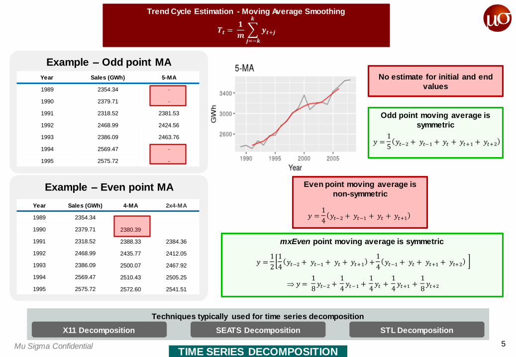
Example – Odd point MA

TIME SERIES DECOMPOSITION

Trend Cycle Estimation - Moving Average Smoothing

𝑻𝒕 =𝟏

𝒎

𝒋=−𝒌

𝒌

𝒚𝒕+𝒋

Year Sales (GWh) 5-MA

1989 2354.34 -

1990 2379.71 -

1991 2318.52 2381.53

1992 2468.99 2424.56

1993 2386.09 2463.76

1994 2569.47 -

1995 2575.72 -

No estimate for initial and end

values

Example – Even point MA

Year Sales (GWh) 4-MA 2x4-MA

1989 2354.34

1990 2379.71 2380.39

1991 2318.52 2388.33 2384.36

1992 2468.99 2435.77 2412.05

1993 2386.09 2500.07 2467.92

1994 2569.47 2510.43 2505.25

1995 2575.72 2572.60 2541.51

Odd point moving average is

symmetric

𝑦 =1

5𝑦𝑡−2 + 𝑦𝑡−1 + 𝑦𝑡 + 𝑦𝑡+1 + 𝑦𝑡+2

Even point moving average is

non-symmetric

𝑦 =1

4𝑦𝑡−2 + 𝑦𝑡−1 + 𝑦𝑡 + 𝑦𝑡+1

mxEven point moving average is symmetric

𝑦 =1

2

1

4𝑦𝑡−2 + 𝑦𝑡−1 + 𝑦𝑡 + 𝑦𝑡+1 +

1

4𝑦𝑡−1 + 𝑦𝑡 + 𝑦𝑡+1 + 𝑦𝑡+2

𝑦 =1

8𝑦𝑡−2 +

1

4𝑦𝑡−1 +

1

4𝑦𝑡 +

1

4𝑦𝑡+1 +

1

8𝑦𝑡+2

Techniques typically used for time series decomposition

X11 Decomposition SEATS Decomposition STL Decomposition

6Mu Sigma ConfidentialBASIC FORECASTING METHOD

BASIC FORECASTING METHOD

Average Method

Future values are same as average of the historical values

Naïve Method

Future values are same as last observation – also called as

random walk forecast

Seasonal Naïve Method

Future values are same as last season value – for e.g. future Feb value will be same as last year’s

Feb value

Drift Method

Future value are same as average change seen over time

in historical data

Average Method

𝑌𝑇+ℎ =𝑦1 + 𝑦2 + …+ 𝑦𝑇−1+ 𝑦𝑇

𝑇

Naïve Method

𝑌𝑇+ℎ = 𝑦𝑇

Seasonal Naïve Method

𝑌𝑇+ℎ =𝑌𝑇+ℎ −𝑚(𝑘+1)

Drift Method

𝑌𝑇+ℎ = 𝑦𝑇 +ℎ𝑦𝑇 − 𝑦1𝑇 − 1

7Mu Sigma ConfidentialBASIC FORECASTING METHOD

FORECASTING USING TIME SERIES DECOMPOSITION

Forecast Seasonal ComponentForecast Seasonally Adjusted

Component

Any non-seasonal forecasting method, like non-seasonal ARIMA, random walk with drift etc. can be used to forecast the

seasonally adjusted component

Seasonal Naïve is typically used to forecast seasonal component assuming

seasonal component doesn’t change much over time

8Mu Sigma ConfidentialEXPONENTIAL SMOOTHING

Forecasts produced using exponential smoothing methods are weighted averages of past observations, with the weights

decaying exponentially as the observations get older. In other words, the most recent observation would have highest weight and the older observations would have lower associated weight

Simple Exponential Smoothing(SES)

▪ Used when time series doesn’t have trend

and seasonality in it i.e. values hover

around the mean

▪ Flat forecast – i.e. all forecast values take

same value

ෝ𝒚𝑻+𝟏 = 𝜶𝒚𝑻 + 𝟏− 𝜶 ෝ𝒚𝑻

ෝ𝒚𝑻+𝟏 = ෝ𝒚𝑻 + 𝜶(𝒚𝑻 − ෝ𝒚𝑻)

0<α<1 is the smoothing parameter

• Forecast for new period is equal to last

smoothed (i.e. fitted) observation plus

some adjusted of error in last fitted and

actual observation

• Parameter is estimated by minimizing the

SSE

Let’s see

an

example

Month Sales (Billions) Alpha = 0.6

Jan-17 97.60 -

Feb-17 95.10 97.60

Mar-17 90.30 96.10

Apr-17 92.50 92.62

May-17 94.60 92.55

Jun-17 91.00 93.78

Jul-17 90.20 92.11

Aug-17 93.00 90.96

Sep-17 93.80 92.19

Oct-17 97.00 93.15

Nov-17 99.00 95.46

Dec-17 90.00 97.58

Jan-18 90.10 93.03

Feb-18 94.20 91.27

Mar-18 95.00 93.03

Apr-18 96.70 94.21

May-18 98.00 95.70

Jun-18 99.00 97.08

84

86

88

90

92

94

96

98

100

JA

N-

17

FE

B-

17

MA

R-1

7

AP

R-

17

MA

Y-

17

JU

N-1

7

JU

L-

17

AU

G-

17

SE

P-

17

OC

T-1

7

NO

V-

17

DE

C-1

7

JA

N-

18

FE

B-

18

MA

R-1

8

AP

R-

18

MA

Y-

18

JU

N-1

8

SIM PLE EXPON ENTIAL SM O OTHING

Actual Predicted

1-Step-Ahead

Forecast

Component form

▪ Forecast Equation

ෝ𝒚𝑻+𝒉 = 𝒍𝑻

▪ Smoothing Equation

𝒍𝑻 = 𝜶𝒚𝑻 + (𝟏 − 𝜶)𝒍𝑻−𝟏


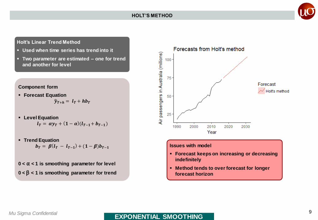
Holt’s Linear Trend Method

▪ Used when time series has trend into it

▪ Two parameter are estimated – one for trend

and another for level

Component form


ෝ𝒚𝑻+𝒉 = 𝒍𝑻+ 𝒉𝒃𝑻

▪ Level Equation

𝒍𝑻 = 𝜶𝒚𝑻 + 𝟏− 𝜶 (𝒍𝑻−𝟏+𝒃𝑻−𝟏)

▪ Trend Equation

𝒃𝑻 = 𝜷 𝒍𝑻 − 𝒍𝑻−𝟏 + (𝟏− 𝜷)𝒃𝑻−𝟏

0 < α < 1 is smoothing parameter for level

0 < < 1 is smoothing parameter for trend

Issues with model

▪ Forecast keeps on increasing or decreasing

indefinitely

▪ Method tends to over forecast for longer

forecast horizon

HOLT’S METHOD


HOLT’S METHOD

Holt’s Damped Trend Method

▪ Another parameter is introduced to dampen

the trend over time

▪ Three parameter are estimated – one for

trend, second for level and third for damping

the trend

Component form


ෝ𝒚𝑻+𝒉 = 𝒍𝑻+ (∅ + ∅𝟐 + …+ ∅𝒉)𝒃𝑻

▪ Level Equation

𝒍𝑻 = 𝜶𝒚𝑻 + 𝟏 −𝜶 (𝒍𝑻−𝟏+∅𝒃𝑻−𝟏)

▪ Trend Equation

𝒃𝑻 = 𝜷 𝒍𝑻 − 𝒍𝑻−𝟏 + (𝟏 − 𝜷)∅𝒃𝑻−𝟏



0 < < 1 is damping parameter

▪ Damping parameter equal to 1 leads to Holt’s

linear trend method

▪ Typically value of damping parameter is kept

between 0.8 to 0.98


HOLT WINTER’S METHOD

EXPONENTIAL SMOOTHING

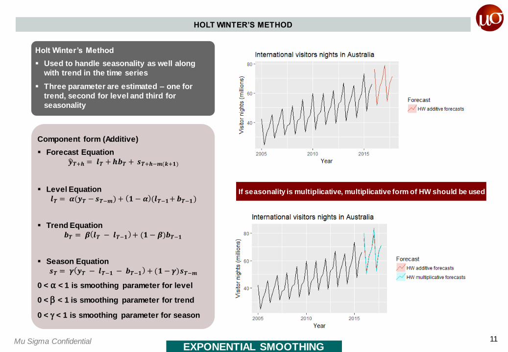
Holt Winter’s Method

▪ Used to handle seasonality as well along

with trend in the time series

▪ Three parameter are estimated – one for

trend, second for level and third for

seasonality

Component form (Additive)


ෝ𝒚𝑻+𝒉 = 𝒍𝑻 +𝒉𝒃𝑻 + 𝒔𝑻+𝒉−𝒎(𝒌+𝟏)

▪ Level Equation

𝒍𝑻 = 𝜶(𝒚𝑻 −𝒔𝑻−𝒎) + 𝟏 − 𝜶 (𝒍𝑻−𝟏+𝒃𝑻−𝟏)

▪ Trend Equation

𝒃𝑻 = 𝜷 𝒍𝑻 − 𝒍𝑻−𝟏 + (𝟏 − 𝜷)𝒃𝑻−𝟏

▪ Season Equation

𝒔𝑻 = 𝜸 𝒚𝑻 − 𝒍𝑻−𝟏 − 𝒃𝑻−𝟏 + (𝟏−𝜸)𝒔𝑻−𝒎



0 < < 1 is smoothing parameter for season

If seasonality is multiplicative, multiplicative form of HW should be used


Damping is also possible for both additive and multiplicative HW method

HOLT WINTER’S METHOD



INNOVATIONS – EXPONENTIAL SMOOTHING MODEL


ETS (Error, Trend, Seasonal) Model

▪ These provide prediction intervals along

with point forecasts

▪ Errors could be additive as well as

multiplicative

Forecast is equal to sum of previous period

forecast and adjustment of error associated

with it

ෝ𝒚𝑻+𝟏 = ෝ𝒚𝑻+ 𝜶(𝒚𝑻 −ෝ𝒚𝑻)

ෝ𝒚𝑻+𝟏 = ෝ𝒚𝑻 − 𝜶𝒆𝑻

Error - AdditiveSeasonality

N A M

Trend

N NN NA NM

A AN AA AM

Ad AdN AdA AdM

Error - MultiplicativeSeasonality

N A M

Trend

N NN NA NM

A AN AA AM

Ad AdN AdA AdM

▪ AIC, AICC, BIC values can be used for model

selection

▪ ETS in R (forecast package) estimates all the

parameters and not the forecast directly

▪ The parameters estimated can be used to

forecast using ‘forecast()’ function

14Mu Sigma ConfidentialARIMA MODEL

ACF AND PACF PLOT

Autocorrelation

▪ It is measure of linear relationship between

current and lagged observation

▪ Graphical representation of autocorrelation

coefficient is called ACF or correlogram

Partial Autocorrelation

▪ It is measure of correlation between current

and lagged observation by excluding

influence of interim observations

▪ Graphical representation of partial

autocorrelation coefficient is called PACF

For series w ith trend and

seasonality, peaks w ill be

observed at seasonal lag –

more like w aves

For series w ith trend only, ACF

w ill gradually move tow ards zero

value

For series w ith trend only, PACF

w ill suddenly drop to zero value

For series w ith trend and

seasonality, PACF w ill show

peaks at seasonal lags

Example Example


MAKING TIME SERIES STATIONARY

Stationary Time Series

▪ A stationary time series doesn’t have any

predictable pattern in long term

▪ Note that cycles are aperiodic and hence,

time series with cycles but no trend and

seasonality will be considered as stationary

Differencing

▪ Differencing helps in stabilizing the mean of

time series by removing changes in level of

the time series

▪ This in turn leads to removal of trend and

seasonality from the data

Non-Stationary

to

Stationary

Non-Stationary Time Series Non-stationarity can be validated from ACF plot

Time Series post First Order Differencing ACF of First Order Differenced Time Series

▪ Box test can be run to identify if original or transformed series is stationary (null hypothesis is of time series being stationary)

▪ Second order differencing, seasonal differencing can also be done

▪ Differencing can also be done post log transformation


AUTO REGRESSIVE INTEGRATED MOVING AVERAGE

Auto Regressive Model

Future values are forecasted by regressing it against linear combination of past values

𝑦𝑡 = 𝑐 + ∅1𝑦𝑡−1+ ∅2𝑦𝑡−2+ …+ ∅𝑛𝑦𝑡−𝑝 + 𝜀𝑡

Above equation would be referred as AR(p) model

Moving Average Model

Future values are forecasted by regressing it against linear combination of forecast errors

𝑦𝑡 = 𝑐 + 𝜃1𝜀𝑡−1+ 𝜃2𝜀𝑡−2+ …+ 𝜃𝑛𝜀𝑡−𝑞 + 𝜀𝑡

Above equation would be referred as MA(q) model

ARIMA Integration

Opposite of differencing

Expressing AR(p) as MA() and MA(q) as AR() is called invertibility of the model; this is an important property of ARIMA model along with stationarity

Value of p and q can be identified using ACF and PACF plots

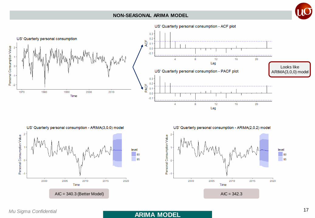
For an ARIMA(p,d,0) model, ACF and PACF plots of

differenced data would show:

▪ ACF exponentially decaying or sinusoidal

▪ Significant spike at lag p in the PACF, but non beyond p

For an ARIMA(0,d,q) model, ACF and PACF plots of

differenced data would show:

▪ PACF exponentially decaying or sinusoidal

▪ Significant spike at lag q in the ACF, but non beyond q

If both p and q are positive, then plots don’t help in finding value of p and q


NON-SEASONAL ARIMA MODEL

Looks like ARIMA(3,0,0) model

AIC = 340.3 (Better Model) AIC = 342.3


Non Seasonal Part of the Model

(p, d, q)

Seasonal Part of the Model

(P, D, Q)m

Seasonal ARIMA

Model

(p, d, q) are estimated using ACF and PACF plots as discussed previously

(P, D, Q) are estimated by observing peaks at the seasonal lags in ACF and PACF plots. For e.g.

ARIMA(0,0,0)(0,0,1)12 model will show:

• A spike at lag 12 of the ACF plot but no other significant peaks

• Exponential decay in seasonal lags of PACF plot

Differencing Seasonal Lag

Data

with

trend a

nd

seasonalit

y

Non-S

tatio

nary

aft

er

seasonal diffe

rencin

g

Dif

fere

ncin

g S

easo

na

l La

g

Dif

fere

nce

d d

ata

Sta

tionary

aft

er diffe

rencin

g t

he

seasonal la

g d

iffe

rence

▪ With peak at lag of 1 in ACF plot, it can be assumed as MA(1) non-seasonal model whereas peak at lag 4 suggests MA(1) seasonal model

▪ Therefore, the model could be ARIMA(0,1,1)(0,1,1)4

▪ Taking PACF plot as reference, ARIMA(1,1,0)(1,1,0)4 can also be created

ARIMA MODEL


SEASONAL ARIMA MODEL

ARIMA MODEL

▪ PACF plot has peaks at seasonal lags of 12, 24; hence, a seasonal AR(1) model can be created

▪ PACF plot also has peaks at 1, 2 and 3; hence, a non-seasonal AR(3) model can be created

▪ Nothing is coming out of ACF plot

▪ Therefore, creating ARIMA(3,0,0)(1,1,0)12

model

Data

with

trend a

nd

multi

plic

ativ

e

seasonalit

y

1

Log t

ransfo

rmatio

n t

o m

ake

seasonalit

y c

onsis

tent

2

Diffe

rencin

g logged d

ata

at

seasonal la

g o

f 12

3


Seasonal ARIMA based on observations made from ACF

and PACF plot

AIC = -464.48

SEASONAL ARIMA MODEL

ARIMA MODEL

Seasonal ARIMA using ‘auto.arima’ function in R

AIC = -486.99

Observations to be made

1)Time Series residuals look like white noise; 2)NO autocorrelation in residuals as per ACF plot; 3)Residuals follow bell curve


ARIMAX / DYNAMIC TIME SERIES MODEL

ARIMAX MODEL

ARIMAX is the extended version of ARIMA model which also includes external regressor into the modelD

aily

ele

ctr

icity

dem

and and

max t

em

pera

ture

tim

e s

eries

Quadra

tic r

ela

tionship

b/w

Dem

and

and tem

pera

ture

Assessing the model f it Forecast for next 14 w eeks

Future values of independent variables are required to

get the forecast; these can also be modeled separately

22Mu Sigma ConfidentialCROSTON MODEL

CROSTON MODEL

▪ Demand Series (q) – Series with non-

zeroes value

▪ Inter-Arrival Time Series (a) – Series

with periods between non-zero values

Application Croston Decomposition Forecasting Model

▪ Extensively used to model

the intermittent demand (multiple zero values) time

series

▪ Simple exponential smoothening

(SES) is done for q and a both

ෝ𝒚𝑻+𝒉 =𝒒𝒋+𝟏

𝒂𝒋+𝟏

j is the time for last observed positive

value

Year Jan Feb Mar Apr May Jun Jul Aug Sep Oct Nov Dec

1 0 2 0 1 0 11 0 0 0 0 2 0

2 6 3 0 0 0 0 0 7 0 0 0 0

3 0 0 0 3 1 0 0 1 0 1 0 0

i 1 2 3 4 5 6 7 8 9 10 11

q 2 1 11 2 6 3 7 3 1 1 1

a 2 2 2 5 2 1 6 8 1 3 2

Croston Decomposition into

Demand and Inter-arrival time

series

Croston model

Prediction intervals are not generated in the Croston methodDoesn’t give point forecast; forecast value is average forecast for the

period


Typically used accuracy metrics

MODEL SELECTION

MODEL FORECAST ACCURACY ASSESSMENT

Root Mean Squared Error

(RMSE)

Mean Absolute Error

(MAE)

Mean Absolute Percentage Error

(MAPE)

Mean Absolute Scaled Error

(MASE)

𝒎𝒆𝒂𝒏(𝒆𝒕𝟐)

▪ Difficult to calculate and

interpret

▪ Forecast method minimizing RMSE will lead to forecasts

of mean

Forecast error IS NOT same as residuals. Forecast error is calculated on test dataset whereas residuals are calculated

on training dataset

𝒆𝑻+𝒉 = 𝒚𝑻+𝒉 − ෝ𝒚𝑻+𝒉

𝒎𝒆𝒂𝒏 𝒆𝒕

▪ Easy to calculate and

interpret

▪ Forecast method minimizing MAE will lead to forecasts

of median

𝒎𝒆𝒂𝒏 𝒑𝒕

▪ Suffers from being equal to

infinite or undefined for yt = 0 or very small I value

𝒎𝒆𝒂𝒏𝒆𝒕

𝑻𝒓𝒂𝒊𝒏𝒊𝒏𝒈𝑴𝑨𝑬

▪ Extended version of MAPE

▪ Value greater than 1 means forecast is better than naïve

forecast and vice versa

Can’t be used when multiple time series

are available with different units as these metrics preserve the metric information

Can be used when multiple time series

are available with different units

At times different accuracy metrics may show different models to be best. In such a scenarios, select model based on business

context

24Mu Sigma ConfidentialMODEL SELECTION

MODEL FORECAST ACCURACY ASSESSMENT

Traditional Test and Train

Sampling

▪ Segregate data into test and

train sample

▪ Typically the split between

train and test is taken as 80-20% or 75-25% of

observations respectively

▪ Model is trained on full

training dataset and

forecast accuracy is

measured on test dataset

Time Series Cross Validation

▪ Multiple test sets are

created with one

observation each

▪ All the observations before

the test observation forms the training set

▪ Model is trained on the training set

▪ Model forecast accuracy is measured by averaging

value over different test sets

▪ The accuracy values

generated are more robust

to be communicated

Train Sample

(In-Sample)

Test Sample

(Held-out Sample)

A good way to choose the best forecasting model is to find the model with the smallest RMSE computed using time series cross-

validation

Time Series Forecasting

Documents

Transcript of Time Series Forecasting