Financial time series forecasting using support

vector machinesAuthor: Kyoung-jae Kim

2003 Elsevier B.V.

Outline

• Introduction to SVM

• Introduction to datasets

• Experimental settings

• Analysis of experimental results

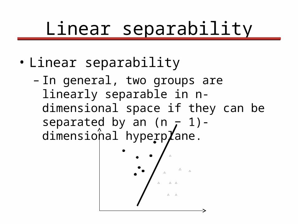
Linear separability

• Linear separability– In general, two groups are linearly separable in n-

dimensional space if they can be separated by an (n − 1)-dimensional hyperplane.

Support Vector Machines

• Maximum-margin hyperplanemaximum-margin hyperplane

Formalization

• Training data

• Hyperplane

• Parallel bounding hyperplanes

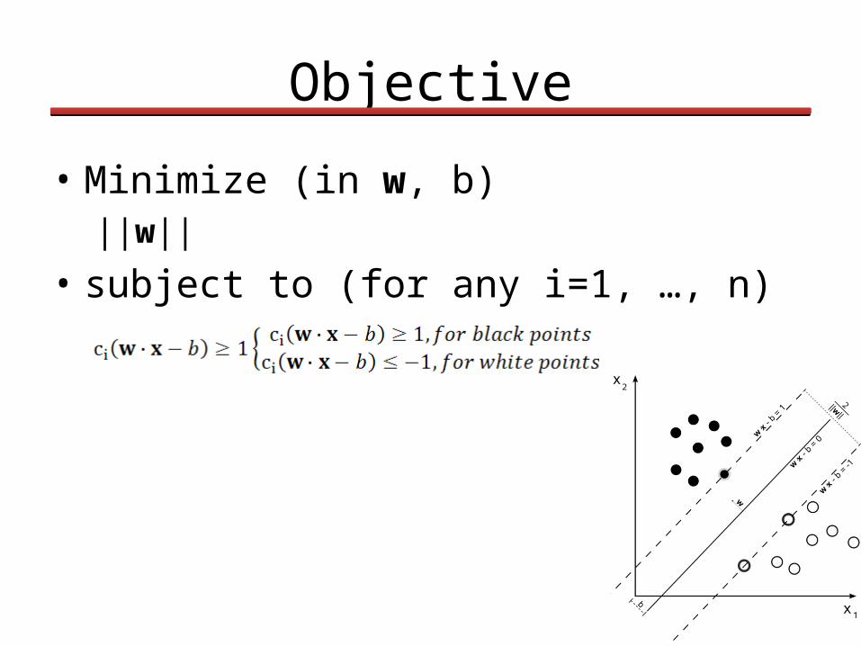
Objective

• Minimize (in w, b)||w||

• subject to (for any i=1, …, n)

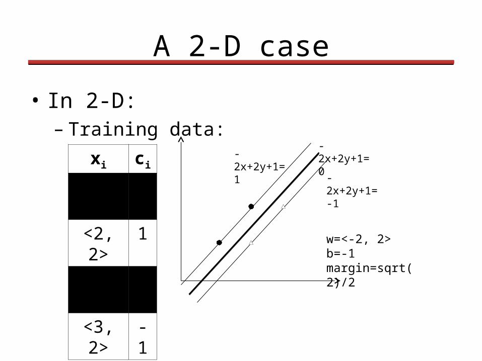
A 2-D case

• In 2-D:– Training data:

xi ci<1, 1> 1<2, 2> 1<2, 1> -1<3, 2> -1

-2x+2y+1=-1

-2x+2y+1=1-2x+2y+1=0

w=<-2, 2>b=-1margin=sqrt(2)/2

Not linear separable

• No hyperplane can separate the two groups

Soft Margin

• Choose a hyperplane that splits the examples as cleanly as possible

• Still maximizing the distance to the nearest cleanly split examples

• Introduce an error cost Cd*C

Higher dimensions

• Separation might be easier

Kernel Trick

• Build maximal margin hyperplanes in high-dimenisonal feature space depends on inner product: more cost

• Use a kernel function that lives in low dimensions, but behaves like an inner product in high dimensions

Kernels

• Polynomial– K(p, q) = (p•q + c)d

• Radial basis function– K(p, q) = exp(-γ||p-q||2)

• Gaussian radial basis– K(p, q) = exp(-||p-q||2/2δ2)

Tuning parameters

• Error weight– C

• Kernel parameters– δ2

– d

– c0

Underfitting & Overfitting

• Underfitting

• Overfitting

• High generalization ability

Datasets

• Input variables– 12 technical indicators

• Target attribute– Korea composite stock price index (KOSPI)

• 2928 trading days– 80% for training, 20% for holdout

Settings (1/3)

• SVM– kernels• polynomial kernel

• Gaussian radial basis function– δ2

– error cost C

Settings (2/3)• BP-Network– layers

• 3– number of hidden nodes

• 6, 12, 24– learning epochs per training example

• 50, 100, 200– learning rate

• 0.1– momentum

• 0.1– input nodes

• 12

Settings (3/3)

• Case-Based Reasoning– k-NN• k = 1, 2, 3, 4, 5

– distance evaluation• Euclidean distance

Experimental results

• The results of SVMs with various C where δ2 is fixed at 25

• Too small C• underfitting*

• Too large C• overfitting*

* F.E.H. Tay, L. Cao, Application of support vector machines in -nancial time series forecasting, Omega 29 (2001) 309–317

Experimental results

• The results of SVMs with various δ2 where C is fixed at 78

• Small value of δ2

• overfitting*

• Large value of δ2

• underfitting*

* F.E.H. Tay, L. Cao, Application of support vector machines in -nancial time series forecasting, Omega 29 (2001) 309–317

Experimental results and conclusion

• SVM outperformes BPN and CBR

• SVM minimizes structural risk

• SVM provides a promising alternative for financial time-series forecasting

• Issues– parameter tuning