Time Series and Forecasting Lecture 2 Nowcasting, Forecast ...bhansen/crete/crete2.pdf · Then a...

Time Series and ForecastingLecture 2

Nowcasting, Forecast Combination,Variance Forecasting

Bruce E. Hansen

Summer School in Economics and EconometricsUniversity of CreteJuly 23-27, 2012

Bruce Hansen (University of Wisconsin) Forecasting July 23-27, 2012 1 / 106

Today’s Schedule

Review

VARs

Nowcasting

Combination Forecasts

Variance Forecasting


Review

Optimal point forecast of yn+1 given information In is the conditionalmean E (yn+1|In)Linear model E (yn+1|In) ' β′xn is an approximationEstimate linear projections by least-squares

Model selection should focus on performance, not “truth”I Best forecast has smallest MSFEI Unknown, but MSFE can be estimatedI CV is a good estimator of MSFE

Good forecasts rely on selection of leading indicators


Vector Autoregresive Modelsyt is an p vectorxt are other variables (including lags)Ideal point forecast E (yn+1|In)Linear approximation

E (yn+1|In) ' A1yt + A2yt−1 + · · ·+ Akyt−k+1 + Bxt

Vector Autoregression (VAR)

yt+1 = A1yt + A2yt−1 + · · ·+ Akyt−k+1 + Bxt + et+1

Estimation: Least squares

yt+1 = A1yt + A2yt−1 + · · · +Akyt−k+1 + Bxt + et+1

One-Step-Ahead Point forecast

yn+1 = A1yn + A2yn−1 + · · ·+ Akyn−k+1 + Bxn


Vector Autoregresive versus Univariate Models

Let xt = (yt , yt−1, ..., xt )Then a VAR is a set of p regression models

y1t+1 = β′1xt + e1t...

ypt+1 = β′pxt + ept

All variables xt enter symmetrically in each equationSims (1980) argued that there is no a priori reason to include orexclude an individual variable from an individual equation.


Model Selection

Do not view selection as identification of “truth”

Rather, inclusion/exclusion is to improve finite sample performanceI minimize MSFE

Use selection methods, equation-by-equation


Example: VAR with 2 variables

y1t+1 = β11y1t + β12y1t−1 + β13y2t + e1t...

y2t+1 = β21y1t + β22y2t + β23y2t−1 + e2t

Selection picks y1t , y1t−1, y2t for equation for y1t+1Selection picks y1t , y2t , y2t−1 for equation for y2t+1The two equations have different variables


Same as system

yt+1 = A1yt + A2yt−1 + et+1

with

A1 =

[β11 β13β21 β22

]A2 =

[β12 00 β23

]The VAR system notation is still quite useful for many purposes(including multi-step forecasting)


Nowcasting

Forecasting current, near recent, or near future economic activity

For example, 2nd quarter GDP (April-June 2012)I So far, we have used information up through first quarterI We have a fair amount of informationI Quite a lot about the 2nd quarter itself


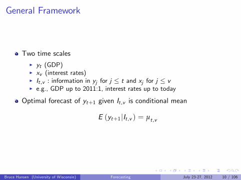
General Framework

Two time scalesI yt (GDP)I xv (interest rates)I It ,v : information in yj for j ≤ t and xj for j ≤ vI e.g., GDP up to 2011:1, interest rates up to today

Optimal forecast of yt+1 given It ,v is conditional mean

E (yt+1|It ,v ) = µt ,v


Standard Linear Approximation

Approximate conditional mean as linear and Markov

E (yt+1|It ,v ) = µt ,v≈ β0 + β1yt + · · ·+ βkyt−k+1

+γ0xv + γ1xv−1 + · · ·+ γpxv−p

Traditional solution (aggregate xv to frequency t)I Sets γj = 0 for periods v before quarter tI Sets γj = γk for periods j and k in common quarter tI Unreasonable restrictions

Unrestricted approximationI Non-parsimoniousI p may be very large


MIDAS

Ghysels, Santa-Clara, and Valkanov

Use parametric distributed-lag structure for coeffi cients γjDiffi cult to justify parametric restrictions


Example: GDP Nowcasting

Suppose we are interested in forecasting 2012 2nd quarter GDPgrowth

I Economic activity for April, May and June

For April, May and June, we have considerable informationI Interest ratesI unemployment ratesI Industrial ProductionI Housing startsI Building PermitsI Inflation


Growth Rate

xt = ln IPt − ln IPt−1


One Month Inflation Rate

INFt = lnCPIt − lnCPIt−1


Three Month Inflation Rate



One Year Inflation Rate



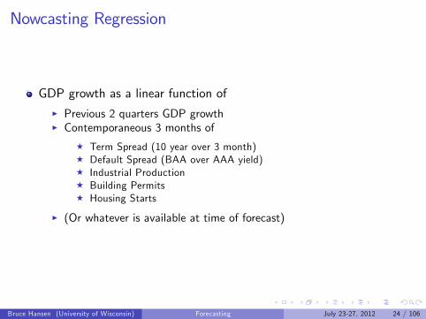
Nowcasting Regression

GDP growth as a linear function ofI Previous 2 quarters GDP growthI Contemporaneous 3 months of

F Term Spread (10 year over 3 month)F Default Spread (BAA over AAA yield)F Industrial ProductionF Building PermitsF Housing Starts

I (Or whatever is available at time of forecast)


Notation

t = year

q = quarter , q = 1, 2, 3, 4

m = month in quarter, m = 1, 2, 3

GDPt ,q= GDP in year t, quarter qI Convention: GDPt ,0 = GDPt−1,4

IPt ,q,m = IP in year t, quarter q, month m


Example Models

Monthly Data through First Month of Forecast Quarter

GDPt ,q = β1GDPt ,q−1 + β2GDPt ,q−2 + β3IPt ,q,1 + β4IPt ,q−1,3 + · · ·

Monthly Data through Second Month of Forecast Quarter

GDPt ,q = β1GDPt ,q−1 + β2GDPt ,q−2 + β3IPt ,q,2 + β4IPt ,q,1 + · · ·

Regressor Construction from Monthly VariablesI Divide into “first”, “second”and “third”months of quartersI Now you have 3 quarterly observations for each variable


Nowcasting Estimates

Based on data through April (first month of forecast quarter)

Selected variables:I ∆ log(GDPt ) (one lag)I IP1, IP3, IP2 (first, previous third, and previous second months)I HS1, HS3 (first and previous third months)

β s(β)Intercept 0.32 (0.62)∆ log(GDPt ) -0.07 (0.06)Industrial Production1 0.17 (0.02)Industrial Production3 0.07 (0.02)Industrial Production2 0.12 (0.03)Housing Starts1 4.00 (1.14)Housing Starts3 −2.64 (1.14)


Nowcasting Point Forecast

2nd Quarter GDP Growth: 2.93

Fitted model: CV = 5.339I Note that yesterday’s best fitting model had CV = 10.28I Point forecast changes from 1.53 to 2.93I Adding contemporaneous IP very useful


Flexibility

As each piece of information becomes available, that variable can beadded to regression

Sequence of nowcast estimates, updated with new information


Recommendation

Make use of higher frequency information

Be creative and flexible

Handling high-dimensional p is similar to many otherhigh-dimensional problems

I Model selection, combination, shrinkgae

Requires frequent re-estimation of distinct forecasting models as newinformation arises

I Requires significant empirical care and attention to detail


Combination Forecasts


Diversity of Forecasts

Model choice is criticalI Classic approach: SelectionI Modern approach: Combination

Issues:I How to select from a wide set of models/forecasts?

F Model selection criteria

I How to combine a wide set of models/forecasts?

F Weight selection criteria


Foundation

The ideal point forecast minimizes the MSFE

The goal of a good combination forecast is to minimize the MSFE


Forecast Selection

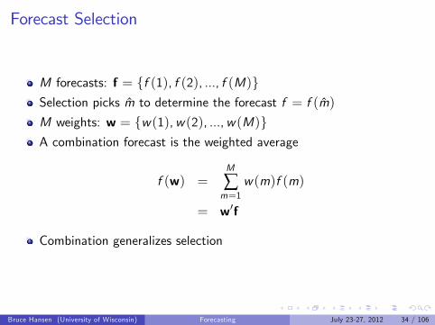
M forecasts: f = f (1), f (2), ..., f (M)Selection picks m to determine the forecast f = f (m)

M weights: w = w(1),w(2), ...,w(M)A combination forecast is the weighted average

f (w) =M

∑m=1

w(m)f (m)

= w′f

Combination generalizes selection


Possible restrictions on the weight vector

∑Mm=1 w(m) = 1I UnbiasednessI Typically improves performance

w(m) ≥ 0I nonnegativityI regularizationI Often critical for good performance

w(m) ∈ 0, 1I Equivalent to forecast selectionI f (w) = f (m)I Selection is a special case of combinationI Strong restriction


OOS Forecast Combination

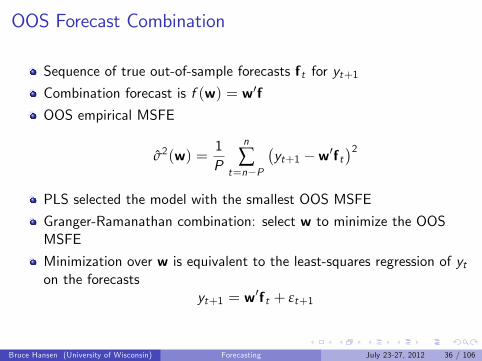
Sequence of true out-of-sample forecasts ft for yt+1Combination forecast is f (w) = w′fOOS empirical MSFE

σ2(w) =1P

n

∑t=n−P

(yt+1 −w′ft

)2PLS selected the model with the smallest OOS MSFE

Granger-Ramanathan combination: select w to minimize the OOSMSFE

Minimization over w is equivalent to the least-squares regression of yton the forecasts

yt+1 = w′ft + εt+1


Granger-Ramanathan (1984)

Unrestricted least-squares

w =

(n

∑t=n−P

ft f ′t

)−1 n

∑t=n−P

ftyt+1

This can produce weights far outside [0, 1] and don’t sum to one

Granger-Ramanathan’s intuition was that this flexibility is goodI But they provided no theory to support conjecture

Unrestricted weights are not regularizedI This results in poor sampling performance


Alternative Representation

Take yt+1 = w′ft + εt+1, subtract yt+1 from each side

0 = w′ft − yt+1 + εt+1

Impose restriction that weights to sum to one.

0 = w′ (ft − yt+1) + εt+1

Define et+1 = w′ (ft − yt+1) , the (negative) forecast errors. Then

0 = w′et+1 + εt+1

This is the regression of 0 on the forecast errors

But it is still better to also impose non-negativity w(m) ≥ 0


Constrained Granger-Ramanathan

The constrained GR weights solve the problem

minww′Aw

subject to

M

∑m=1

w(m) = 1

0 ≤ w(m) ≤ 1where

A = ∑tet+1e′t+1

is the M ×M matrix of forecast error empirical variances/covariances


Quadratic Programming (QP)

The weights lie on the unit simplex

The constrained GR weights minimize a quadratic over the unitsimplex

QP algorithms easily solve this problemI Gauss (qprog)I Matlab (quadprog)I R (quadprog)

Solution solution typicalI Many forecasts will receive zero weight


Bates-Granger (1969)

Assume A = ∑t et+1e′t+1 is diagonal.Then the regression with the coeffi cients constrained to sum to one

0 = w′et+1 + εt+1

has solution

w(m) =σ−2(m)

∑Mj=1 σ−2(j)

This are the Bates-Granger weights.

In many cases, they are close to equality, since OOS forecastvariances can be quite similar


Bayesian Model Averaging (BMA)

Put priors on individual models, and priors on the probability thatmodel m is the true model

Compute posterior probabilites w(m) that m is the true model

Forecast combination using w(m)

AdvantagesI Conceptually simpleI no theoretical analysis requiredI applies in broad contexts

DisadvantagesI Not designed to minimize forecast riskI Similar to BIC: asymptotically picks “true”finite modelsI does not distinguish between 1-step and multi-step forecast horizons


BMA Approximation

BIC weights

w(m) ∝ exp(−BIC (m)

2

)Simple approximation to full BMA method

Smoothed version of BIC selection

Works better than BIC selection in simulations


AIC Weights

Smooted AIC

w(m) ∝ exp(−AIC (m)

2

)Proposed by Buckland, Burnhamm and Augustin (1997)

Not theoretically motivated, but works better than AIC selection insimulations


Comments

Combination methods typically work better (lower MSFE) thancomparable selection methods

BIC and BMA not optimal for MSFE

Granger-Ramanathan has similar senstive as PLS to choice of P

Bates-Granger and weighted AIC have no theoretical grounding


Forecast Combination

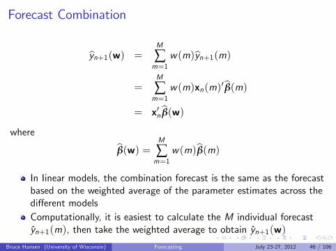
yn+1(w) =M

∑m=1

w(m)yn+1(m)

=M

∑m=1

w(m)xn(m)′ β(m)

= x′n β(w)

where

β(w) =M

∑m=1

w(m)β(m)

In Iinear models, the combination forecast is the same as the forecastbased on the weighted average of the parameter estimates across thedifferent modelsComputationally, it is easiest to calculate the M individual forecastyn+1(m), then take the weighted average to obtain yn+1(w)


Combination Residuals

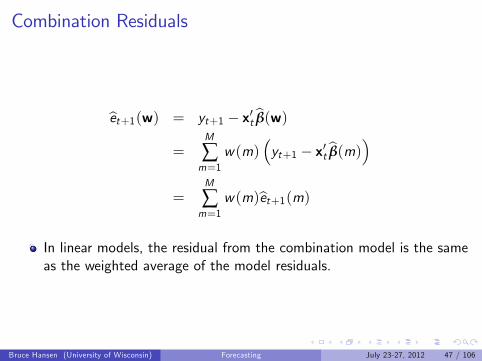
et+1(w) = yt+1 − x′t β(w)

=M

∑m=1

w(m)(yt+1 − x′t β(m)

)=

M

∑m=1

w(m)et+1(m)

In linear models, the residual from the combination model is the sameas the weighted average of the model residuals.


Residual variance

σ2(w) =1n

n

∑t=1

(M

∑m=1

w(m)et+1(m)

)2=

1n

n

∑t=1

(w′et+1

)2= w′Sw

where

S =1n

n

∑t=1et+1e′t+1

The residual variance is a quadratic function of the covariance matrixof the M model residuals.


Point Forecast and MSFE

Given yn+1(w) the forecast error is

yn+1 − yn+1(w) = x′nβ+ et+1 − x′n β(w)

= en+1 − x′n(

β(w)− β)

The mean-squared-forecast-error (MSFE) is

MSFE (w) = E(en+1 − x′n

(β(w)− β

))2' σ2 + E

((β(w)− β

)′Q(

β(w)− β))

Minimizing MSFE is the same as minimizing the MSE of thecoeffi cient estimate


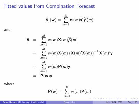
Fitted values from Combination Forecast

µt (w) =M

∑m=1

w(m)x′t β(m)

and

µ =M

∑m=1

w(m)X(m)β(m)

=M

∑m=1

w(m)X(m)(X(m)′X(m)

)−1 X(m)′y=

M

∑m=1

w(m)P(m)y

= P(w)y

where

P(w) =M

∑m=1

w(m)P(m)


Fitted values from Combination Forecast (con’t)

µ = P(w)y

P(w) =M

∑m=1

w(m)P(m)

In-sample fitted values are a linear operator on the dependent variable

The operator P(w) is not a projection matrixIt is a weighted average of projection matrices


Residual Fit

σ(w)2 =1n

n−1∑t=0

et+1(w)2

=1n

n−1∑t=0

e2t+1 +1n

n−1∑t=0

(x′t(

β(w)− β))2

−2n

n−1∑t=0

et+1x′t(

β(w)− β)

First two terms are estimates of

MSFE (w) = E(en+1 − x′n

(β(w)− β

))2


Third term is

n−1∑t=0

et+1x′t(

β(w)− β)=

M

∑m=1

w(m)n−1∑t=0

et+1x′t(

β(m)− β)

=M

∑m=1

w(m)e′P(m)e

= e′P(w)e

whereP(m) = X(m)

(X(m)′X(m)

)−1 X(m)′and

P(w) =M

∑m=1

w(m)P(m)


Residual Variance as Biased estimate of MSFE

E(σ(w)2

)' MSFEn(w)−

2nB(w)

where

B(w) = E(e′P(w)e

)=

M

∑m=1

w(m)E(e′P(m)e

)=

M

∑m=1

w(m)B(m)

Unbiased estimate of MSFE

Cn(w) = σ(w)2 +2nB(w)


Bias Term

B(w) =M

∑m=1

w(m)B(m)

B(m) = tr(Q(m)−1Ω(m)

)In homoskedastic case

B(m) = σ2k(m)

B(w) = σ2M

∑m=1

w(m)k(m)

a weighted average of the number of coeffi cients in each estimator.


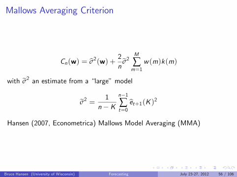
Mallows Averaging Criterion

Cn(w) = σ2(w) +2n

σ2M

∑m=1

w(m)k(m)

with σ2 an estimate from a “large”model

σ2 =1

n−Kn−1∑t=0

et+1(K )2

Hansen (2007, Econometrica) Mallows Model Averaging (MMA)


Mallows Weight Selection

WriteM

∑m=1

w(m)k(m) = w′K

where K = (k(1), ..., k(M))′. This is linear in wWe showed earlier that σ2(w) = w′Sw is quadratic.Linear/Quadratic criterion

Cn(w) = w′Sw+2n

σ2w′K


Forecast Model Averaging (FMA)

Hansen (Journal of Econometrics, 2008)

Cn(w) = w′Sw+2n

σ2w′K

Combination weights found by constrained minimization of Cn(w)

w = argminw

[w′Sw+

2n

σ2w′K]

subject to

M

∑m=1

w(m) = 1

0 ≤ w(m) ≤ 1Solution by Quadratic Programming (QP)


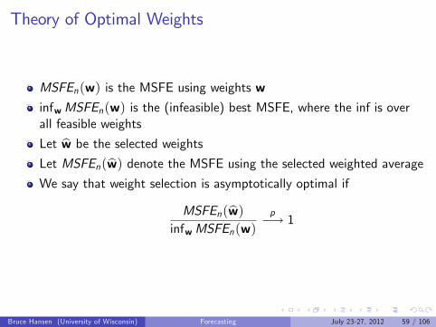
Theory of Optimal Weights

MSFEn(w) is the MSFE using weights winfwMSFEn(w) is the (infeasible) best MSFE, where the inf is overall feasible weights

Let w be the selected weightsLet MSFEn(w) denote the MSFE using the selected weighted averageWe say that weight selection is asymptotically optimal if

MSFEn(w)infwMSFEn(w)

p−→ 1


Theory of Optimal Weights

Hansen (2007, Econometrica)

Mallows weight selection is asymptotically optimal underhomoskedasticity

No optimality proof yet for dependent data


Comparison of Granger-Ramanathan and FMA

Both are solved by Quadratic Programming (QP)

Both typically yield corner solutions —many forecasts will receive zeroweight

GR uses empirical (OOS) forecast errors, FMA uses sample residuals

GR uses no penalty, FMA uses “average # of parameters”penalty

FMA is an estimate of MSFE for homoskedastic one-step forecasts,GR has no optimality


Robust Mallows

Cn(w) = σ2(w) +2n

M

∑m=1

w(m) tr(Q(m)−1Ω(m)

)Q(m) = E

(xt (m)xt (m)′

)Ω(m) = E

(xt (m)x′t (m)e

2t+1

)Sample estimate

C ∗n (w) = σ2(w) +2n

M

∑m=1

w(m) tr(Q(m)−1Ω(m)

)= w′Sw+

2nw′B

where

B =(

tr(Q(1)−1Ω(1)

), tr

(Q(2)−1Ω(2)

),... tr

(Q(K )−1Ω(K )

) )′is vector of correction terms from robust Mallows selection.Bruce Hansen (University of Wisconsin) Forecasting July 23-27, 2012 62 / 106

Cross-Validation

Leave-one-out estimator

β−t (w) =M

∑m=1

w(m)β−t (m)

=M

∑m=1

w(m)

(∑j 6=txj (m)xj (m)′

)−1 (∑j 6=txj (m)yj+1

)

Leave-one-out prediction residual

et+1(m) = yt+1 −M

∑m=1

w(m)β−t (w)′xt (m)

=M

∑m=1

w(m)et+1(m)

where the second equality holds since the weights sum to one.


CVn(w) =1n

∑n−1t=0 et+1(w)

2 is an estimate of MSFEn(m)

Cross-validation (CV) criterion for regression combination/averaging


Cross-validation criterion for combination forecasts

CVn(w) =1n

n

∑t=1et+1(w)2

=1n

n

∑t=1

(M

∑m=1

w(m)et+1(m)

)2

=M

∑m=1

M

∑`=1

w(m)w(`)1n

n

∑t=1et+1(m)et+1(`)

= w′Sw

whereS =

1ne ′e

is covariance matrix of leave-1-out residuals.


Cross-validation Weights

Combination weights found by constrained minimization of CVn(w)

minwCVn(w) = w′Sw

subject to

M

∑m=1

w(m) = 1

0 ≤ w(m) ≤ 1


Cross-validation for combination forecasts (theory)

Theorem: ECVn(w) ' Cn(w)For heteroskedastic forecasts, CV is a valid estimate of the one-stepMSFE from a combination forecast

Hansen and Racine (Journal of Econometrica, 2012) show that theCV weights are asymptotically optimal for cross-section data underheteroskedasticity

No optimality theory for dependent data


Computation (R)

Min (12w′Sw+ d ′w) subject to A′w ≥ b

Need quadprog packageI Install under packagesI library(quadprog)

QP <- solve.QP(D,d,A,b,b)

w <- QP$solution

w <- as.matrix(w)

help(solve.QP) for documentation

D = S = (e ′e)/n where e is n×M matrix of leave-one-out residuals


Summary: Forecast Combination Methods

Granger-Ramanathan (GR), forecast model averaging (FMA) andcross-validation (CV) all pick weight vectors by quadraticminimization

GR only needs actual forecasts, the method can be unknown or ablack box

CV can be computed for a wide variety of estimation methodsI optimality theory for linear estimation

FMA limited to homoskedastic one-step-ahead models

Smoothed AIC (SAIC) and BMA have no forecast optimality, and aredesigned for homoskedastic one-step-ahead forecasts.


Example: AR models for GDP Growth

Fit AR(1) and AR(2) only

Leave-one-out residuals e1t and e2tCovariance matrix

S =[10.72 10.4410.44 10.52

]The best-fitting single model is AR(2)

The best combination is w = (.22, .78)′

CV = 10.50


Example: AR models for GDP Growth

Fit AR(0) through AR(12)

AR(0) is constant only

Models with positive weight are AR(0), AR(1), AR(2)

w = (.06, .16, .78)′

S =

12.0 10.6 10.410.6 10.7 10.410.4 10.5 10.5

CV = 10.50 (essentially unchanged)


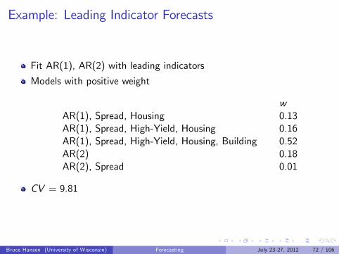
Example: Leading Indicator Forecasts

Fit AR(1), AR(2) with leading indicators

Models with positive weight

wAR(1), Spread, Housing 0.13AR(1), Spread, High-Yield, Housing 0.16AR(1), Spread, High-Yield, Housing, Building 0.52AR(2) 0.18AR(2), Spread 0.01

CV = 9.81


Example: Nowcasting

Models with positive weight areI w = .17 on ∆ log(GDPt ), IP1, IP3, IP2, HS1,I w = .83 on ∆ log(GDPt ), IP1, IP3, IP2, HS1, HS3

CV = 5.335

Point Forecast= 2.91

Essentially same as selected model


Summary: Forecast Combination by CVM forecasts fn+1(m) from n observations

For each estimate mI Define the leave-one-out prediction error

et+1(m) = yt+1 − β′(−t)(m)xt (m)

=et+1(m)1− htt (m)

I Store the n× 1 vector e(m)Construct the M ×M matrix

S =1ne ′e

Find the M × 1 weight vector w which minimizes w′SwI Use quadratic programming (quadprog) to find solution

The combination forecast is fn+1 = ∑Mm=1 w(m)fn+1(m)


Forecast Combination Criticisms

There has been considerable skepticism about formal forecastcombination method in the forecast literature

Many researchers have found that equal weighting: (wm = 1/M)works as well as formal methods

However, the formal methods which investigated areI Bates-Granger simple weights

F Not expected by theory to work well

I Unconstrained Granger-Ramanathan

F Without imposing [0, 1] weights, work terribly!

Furthermore, most investigations examine pseudo out-of-sampleperformance

I Identical to comparing models by PLS criterionI This is NOT an investigation of performanceI Just a ranking by PLS


Another Example - 10-Year Bond Rate

Estimated AR(1) through AR(24) models

CV Selection picked AR(2)

CV weight Selection: Models with positive weightI AR(0): w = 0.04I AR(1): w = 0.04I AR(2): w = 0.47I AR(6): w = 0.23I AR(22): w = 0.22

MInimizing CV = 0.0761 (slightly lower than 0.0768 from AR(2))

Point forecast 1.96 (same as from AR(2))


Variance Forecasting


Variance Forecasts

Forecast uncertaintyI Point forecasts insuffi cient!

σ2t+1 = var (yt+1|It )In the model yt+1 = β′xt + et+1

I σ2t+1 = var (et+1 |In) = E(e2t+1 |It

)


10-Year Bond Rate

Prediction Residuals

Squares


Figure: Leave-One-Out Prediction Residuals

1960 1970 1980 1990 2000 2010

1.5

1.0

0.5

0.0

0.5

1.0

1.5


Figure: Squared Prediction Residuals

1960 1970 1980 1990 2000 2010

0.0

0.5

1.0

1.5

2.0

2.5


Variance Forecast Methods

Constant Variance σ2t = σ2

I Uncertainty not state-dependent

GARCHI Common in financial dataI Estimated by MLE

Regression ApproachI σ2t = E

(e2t+1 |In

)≈ α′xt


2-Step Variance Estimation

Start with residuals et+1I Better choice: leave-one-out residuals et+1

Estimate variance model (constant, ARCH, or regression)

Obtain σ2n from fitted model


Which Residuals?

Least-squares residual variance biased toward zeroI Forecast variance biased towards zero

Leave-one-out residual variance estimates out-of-sample MSFEI This is appropriate


Joint Estimation: Mean and Variance

Alternative to two-step estimationI I prefer 2-step as the regression coeffi cients preserve their projectioninterpretation

I When the model is an approximation, the coeffi cient change theirmeaning under joint estimation


Constant Variance Model

σ2t = σ2

σ2n = σ2 =1

n− 1 ∑n−1t=1 e

2t+1


Regression Variance Model

σ2t ≈ α′xte2t+1 = α′xt + ηt

α =(∑n−1t=1 xtx

′t

)−1 (∑n−1t=1 xt e

2t+1

)σ2n = α′xn

I Easy, but not constrained to (0,∞)


GARCH Models

σ2t = ω+ βσ2t−1 + αe2tConditional variance of et+1Specifies conditional variance as function of recent squaredinnovations

Large innovations (in magnitude) raise conditional variance

Lagged variance smooths σ2t

Non-negativity constraints: ω > 0, β ≥ 0, α > 0


GARCH with Regressors

σ2t = ω+ βσ2t−1 + αe2t + γxtxt > 0 useful to constrain regressor to be positive


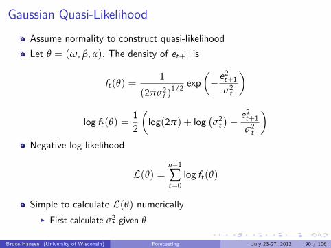
Gaussian Quasi-Likelihood

Assume normality to construct quasi-likelihood

Let θ = (ω, β, α). The density of et+1 is

ft (θ) =1

(2πσ2t )1/2 exp

(−e

2t+1

σ2t

)

log ft (θ) =12

(log(2π) + log

(σ2t)− e

2t+1

σ2t

)Negative log-likelihood

L(θ) =n−1∑t=0

log ft (θ)

Simple to calculate L(θ) numericallyI First calculate σ2t given θ


Gaussian QMLE

QMLE θ minimizes L(θ)I Easy using BFGS or other gradient methodI Constrained optimization can be used to impose non-negativeparameters

Can write L(θ) as a procedure and numerically minimizeI For each θ

F Calculate σ2t by recursion σ2t = ω+ βσ2t−1 + αe2t given σ20F Useful to trim σ2t >> 0F If σ2t ≤ σ20/100 then set σ2t = σ20/100F Calculate log ft (θ) and L(θ)


Computation (R)

Use tseries packageI Install under packagesI library(tseries)

x.arch <- garch(e,order=c(1,1))

x.arch <-garch(e,order=c(1,1),control=garch.control(start=st))

I st=starting values

archc=coef(x.arch)

sd=predict(x.arch)

like=logLik(x.arch)

help(garch)


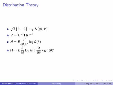
Distribution Theory

√n(

θ − θ)→d N((0,V )

V = H−1ΩH−1

H = E∂2

∂θ∂θ′log ft (θ)

Ω = E∂

∂θlog ft (θ)

∂

∂θlog ft (θ)′


Standard Errors

H =1n

∑n−1t=0

∂2

∂θ∂θ′log ft (θ) =

1n

∂2

∂θ∂θ′L(θ)

Ω =1n

∑n−1t=0

∂

∂θlog ft (θ)

∂

∂θlog ft (θ)′

Both can be calculated numerically

V = H−1ΩH−1

Standard errors are square roots of diagonal elements of n−1V


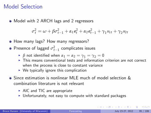
Model Selection

Model with 2 ARCH lags and 2 regressors

σ2t = ω+ βσ2t−1 + α1e2t + α2e2t−1 + γ1x1t + γ2x2t

How many lags? How many regressors?

Presence of lagged σ2t−1 complicates issuesI β not identified when α1 = α2 = γ1 = γ2 = 0I This means conventional tests and information criterion are not correctwhen the process is close to constant variance

I We typically ignore this complication

Since estimation is nonlinear MLE much of model selection &combination literature is not relevant

I AIC and TIC are appropriateI Unfortunately, not easy to compute with standard packages


AIC and TIC for GARCH models

If model m has parameter vector θ(m) with k(m) elements

AIC (m) = 2L(θ(m)) + 2k(m)TIC (m) = 2L(θ(m)) + 2 tr

(H(m)−1Ω(m)

)Not standard output


Variance Forecast from GARCH model

σ2n+1 = ω+ βσ2n + α1e2nσ2n+1 = ω+ βσ2n + α1 e2nσ2n+1 is estimated conditional variance of yn+1

Standard deviation√

σ2n+1


Example: 10-Year Bond Rate

GARCH(1,1)

σ2t = ω+ αe2t + βσ2t−1

Estimate s.e.ω 0.0001 0.0001α 0.200 0.041β 0.835 0.025


Variance Forecast

Conditional varianceI σ2n+1 = 0.054I σn+1 = 0.23

UnconditionalI σ2 = 0.076I σ = 0.28

The conditional variance at present is similar, but somewhat smallerthan the unconditional


Figure: Estimated Variance

1960 1970 1980 1990 2000 2010

0.0

0.2

0.4

0.6

0.8


Example: GDP Growth


Figure: GDP: Leave-One-Out Prediction Residuals

1970 1980 1990 2000 2010

10

50

510


Figure: GDP: Squared Prediction Residuals

1970 1980 1990 2000 2010

050

100

150


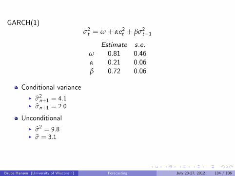
GARCH(1)σ2t = ω+ αe2t + βσ2t−1

Estimate s.e.ω 0.81 0.46α 0.21 0.06β 0.72 0.06

Conditional varianceI σ2n+1 = 4.1I σn+1 = 2.0

UnconditionalI σ2 = 9.8I σ = 3.1


Figure: GDP: Estimated Variance

1970 1980 1990 2000 2010

1020

3040


Assignment 2

Take your regression models from yesterday

Calculate forecast weights by cross-validation (CV).

Use these weights to make a one-step point forecast for July 2012.

Take the leave-one-out prediction residuals. Estimate a GARCH(1,1)model for the residuals. Calculate a one-step forecast standarddeviation from the GARCH model, and compare with theunconditional standard deviation.


Time Series and Forecasting Lecture 2 Nowcasting, Forecast ...bhansen/crete/crete2.pdf · Then a...

Documents

Transcript of Time Series and Forecasting Lecture 2 Nowcasting, Forecast ...bhansen/crete/crete2.pdf · Then a...