Time Series Analysis - Technical University of Denmarkhm/time.series.analysis/slides/lect10.pdf ·...
29
1 Henrik Madsen H. Madsen, Time Series Analysis, Chapmann Hall Time Series Analysis Henrik Madsen [email protected] Informatics and Mathematical Modelling Technical University of Denmark DK-2800 Kgs. Lyngby
Transcript of Time Series Analysis - Technical University of Denmarkhm/time.series.analysis/slides/lect10.pdf ·...
1Henrik Madsen
H. Madsen, Time Series Analysis, Chapmann Hall
Time Series Analysis
Henrik Madsen
Informatics and Mathematical Modelling
Technical University of Denmark
DK-2800 Kgs. Lyngby
2Henrik Madsen
H. Madsen, Time Series Analysis, Chapmann Hall
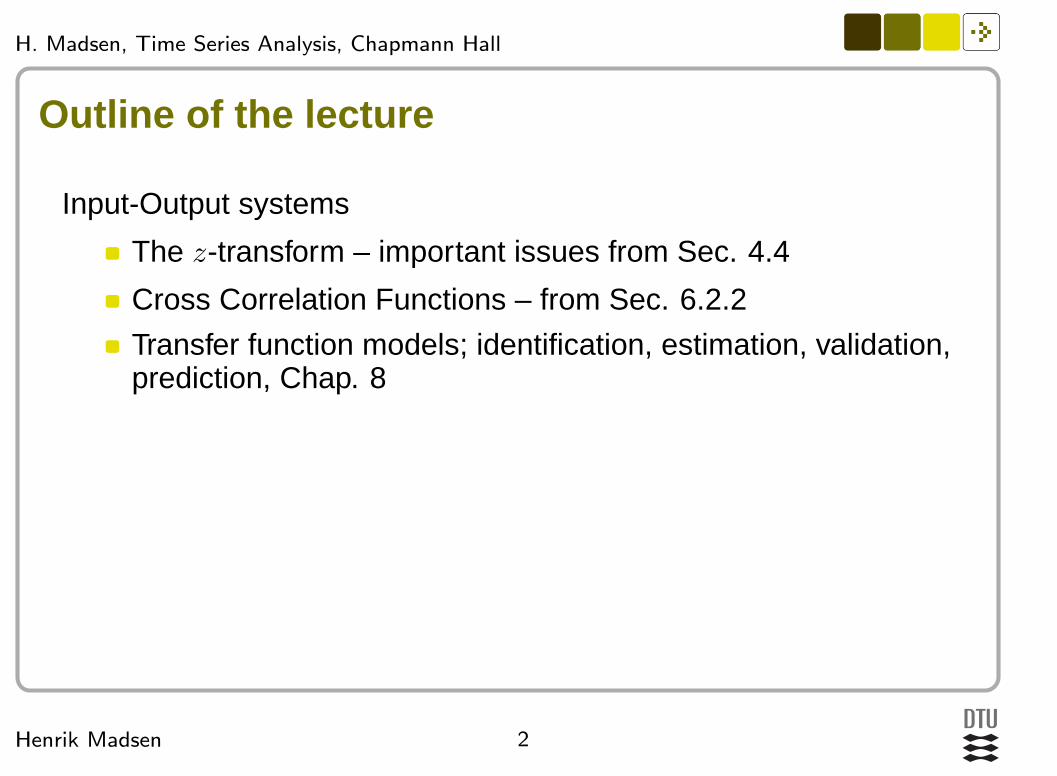
Outline of the lecture
Input-Output systems
The z-transform – important issues from Sec. 4.4
Cross Correlation Functions – from Sec. 6.2.2
Transfer function models; identification, estimation, validation,prediction, Chap. 8

3Henrik Madsen
H. Madsen, Time Series Analysis, Chapmann Hall
The z-transformA way to describe dynamical systems in discrete time
Z({xt}) = X(z) =∞∑
t=−∞
xtz−t (z complex)
The z-transform of a time delay: Z({xt−τ}) = z−τX(z)
The transfer function of the system is called H(z) =
∞∑
t=−∞
htz−t
yt =
∞∑
k=−∞
hkxt−k ⇔ Y (z) = H(z)X(z)
Relation to the frequency response function: H(ω) = H(eiω)
4Henrik Madsen
H. Madsen, Time Series Analysis, Chapmann Hall
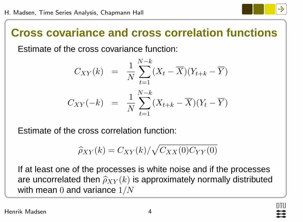
Cross covariance and cross correlation functionsEstimate of the cross covariance function:
CXY (k) =1
N
N−k∑
t=1
(Xt −X)(Yt+k − Y )
CXY (−k) =1
N
N−k∑
t=1
(Xt+k −X)(Yt − Y )
Estimate of the cross correlation function:
ρXY (k) = CXY (k)/√CXX(0)CY Y (0)
If at least one of the processes is white noise and if the processesare uncorrelated then ρXY (k) is approximately normally distributedwith mean 0 and variance 1/N
5Henrik Madsen
H. Madsen, Time Series Analysis, Chapmann Hall
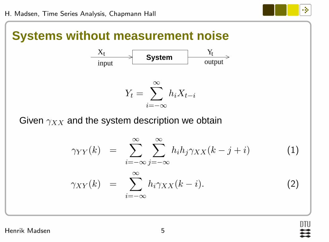
Systems without measurement noise
outputinputSystem tX Yt
Yt =∞∑
i=−∞
hiXt−i
Given γXX and the system description we obtain
γY Y (k) =
∞∑
i=−∞
∞∑
j=−∞
hihjγXX(k − j + i) (1)
γXY (k) =
∞∑
i=−∞
hiγXX(k − i). (2)
6Henrik Madsen
H. Madsen, Time Series Analysis, Chapmann Hall
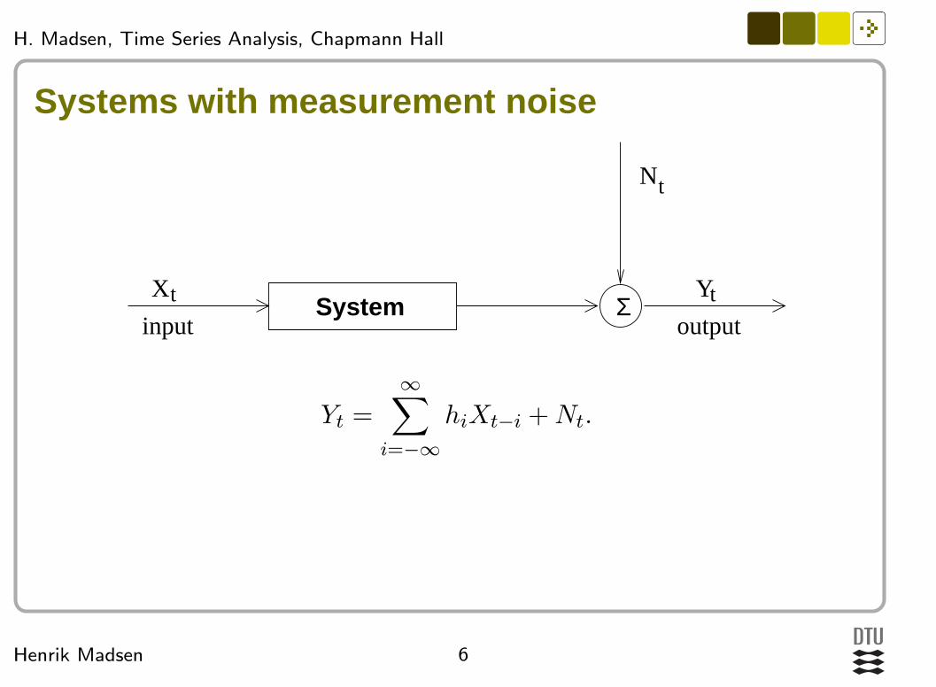
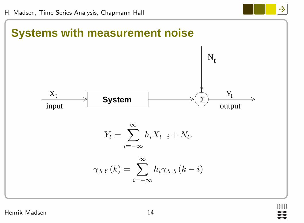
Systems with measurement noise
SystemXt
inputΣ
Yt
tN
output
Yt =∞∑
i=−∞
hiXt−i +Nt.
7Henrik Madsen
H. Madsen, Time Series Analysis, Chapmann Hall
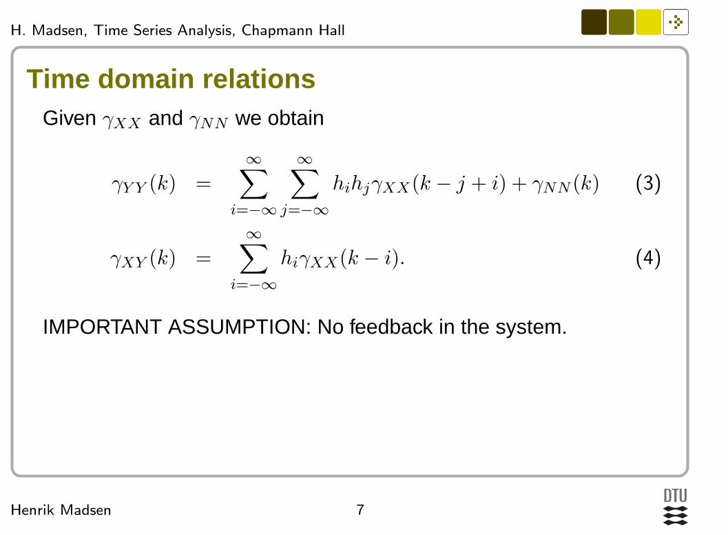
Time domain relationsGiven γXX and γNN we obtain
γY Y (k) =
∞∑
i=−∞
∞∑
j=−∞
hihjγXX(k − j + i) + γNN (k) (3)
γXY (k) =
∞∑
i=−∞
hiγXX(k − i). (4)
IMPORTANT ASSUMPTION: No feedback in the system.
8Henrik Madsen
H. Madsen, Time Series Analysis, Chapmann Hall
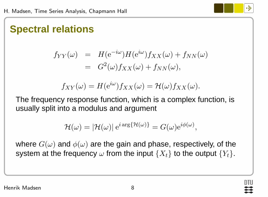
Spectral relations
fY Y (ω) = H(e−iω)H(eiω)fXX(ω) + fNN (ω)
= G2(ω)fXX(ω) + fNN (ω),
fXY (ω) = H(eiω)fXX(ω) = H(ω)fXX(ω).
The frequency response function, which is a complex function, isusually split into a modulus and argument
H(ω) = |H(ω)| ei arg{H(ω)} = G(ω)eiφ(ω),
where G(ω) and φ(ω) are the gain and phase, respectively, of thesystem at the frequency ω from the input {Xt} to the output {Yt}.

9Henrik Madsen
H. Madsen, Time Series Analysis, Chapmann Hall
Estimating the impulse responseThe poles and zeros characterize the impulse response(Appendix A and Chapter 8)
If we can estimate the impulse response from recordings ofinput an output we can get information that allows us tosuggest a structure for the transfer function
Lag
Tru
e Im
puls
e R
espo
nse
0 10 20 30
0.0
0.04
0.08
Lag
SC
CF
0 10 20 30
0.0
0.2
0.4
0.6
Lag
SC
CF
afte
r pr
e−w
hite
ning
0 10 20 30
0.0
0.1
0.2
0.3
0.4
10Henrik Madsen
H. Madsen, Time Series Analysis, Chapmann Hall
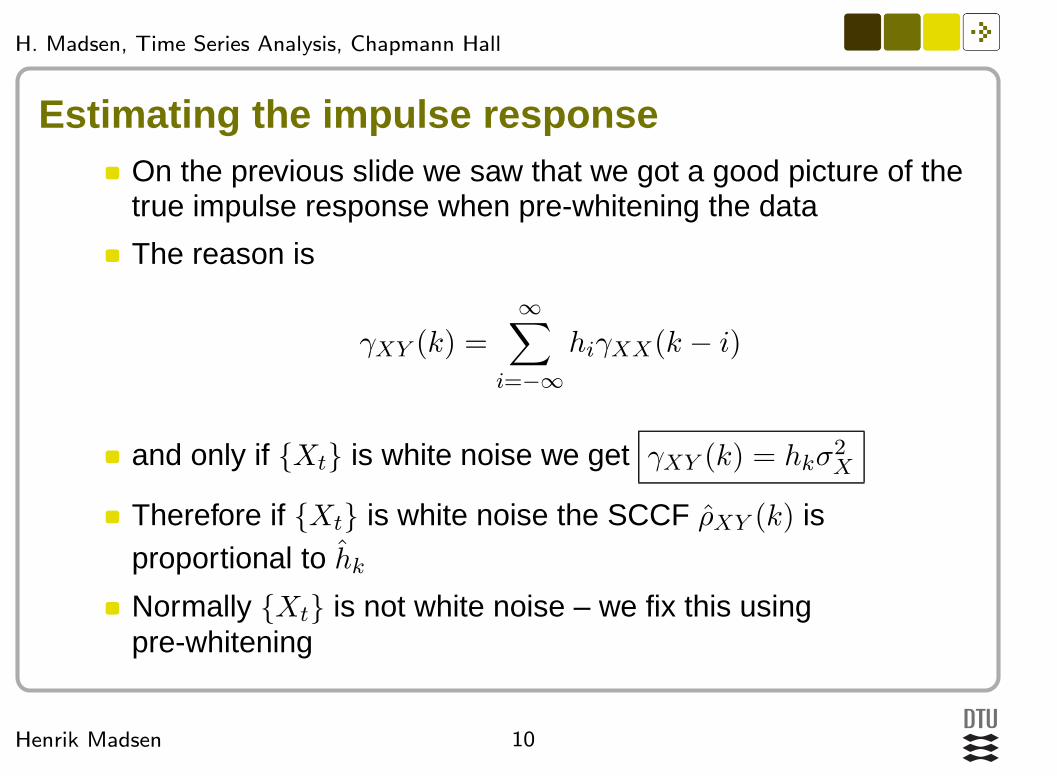
Estimating the impulse responseOn the previous slide we saw that we got a good picture of thetrue impulse response when pre-whitening the data
The reason is
γXY (k) =∞∑
i=−∞
hiγXX(k − i)
and only if {Xt} is white noise we get γXY (k) = hkσ2X
Therefore if {Xt} is white noise the SCCF ρXY (k) isproportional to hk
Normally {Xt} is not white noise – we fix this usingpre-whitening
11Henrik Madsen
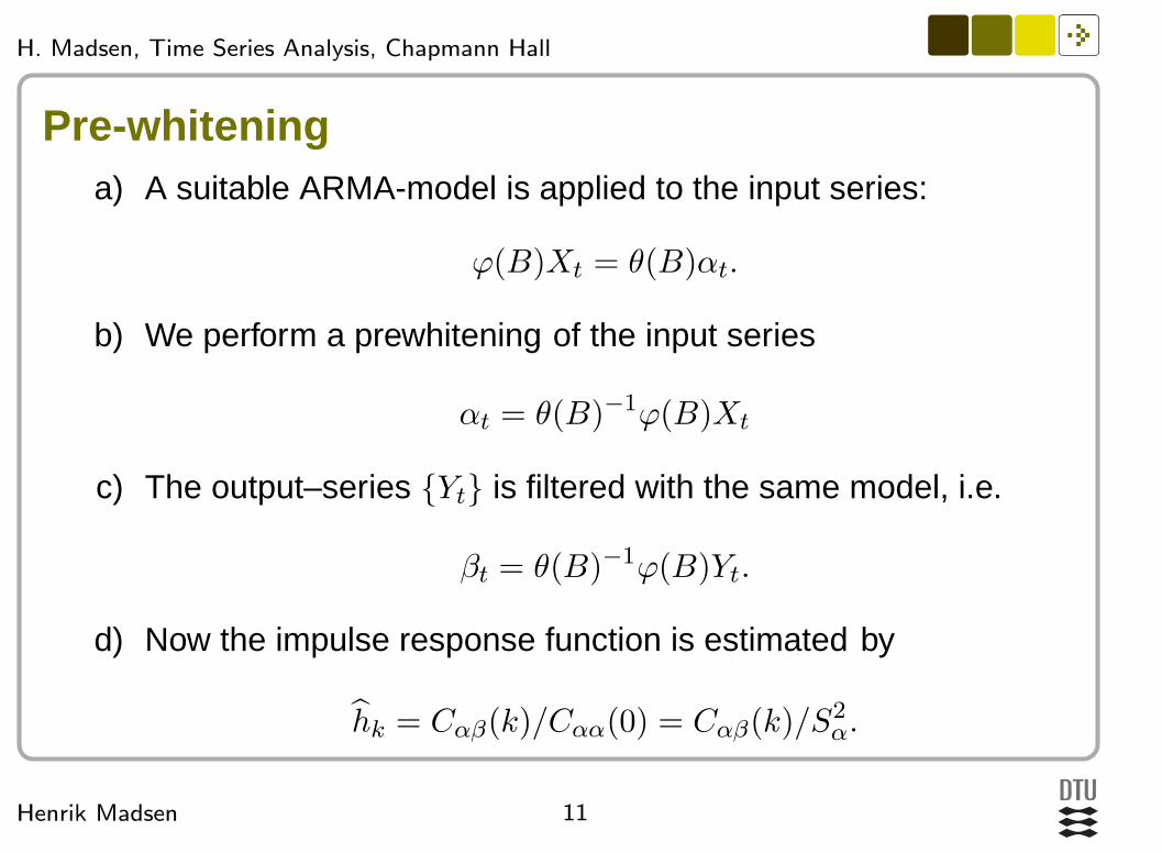
H. Madsen, Time Series Analysis, Chapmann Hall
Pre-whiteninga) A suitable ARMA-model is applied to the input series:
ϕ(B)Xt = θ(B)αt.
b) We perform a prewhitening of the input series
αt = θ(B)−1ϕ(B)Xt
c) The output–series {Yt} is filtered with the same model, i.e.
βt = θ(B)−1ϕ(B)Yt.
d) Now the impulse response function is estimated by
hk = Cαβ(k)/Cαα(0) = Cαβ(k)/S2α.

12Henrik Madsen
H. Madsen, Time Series Analysis, Chapmann Hall
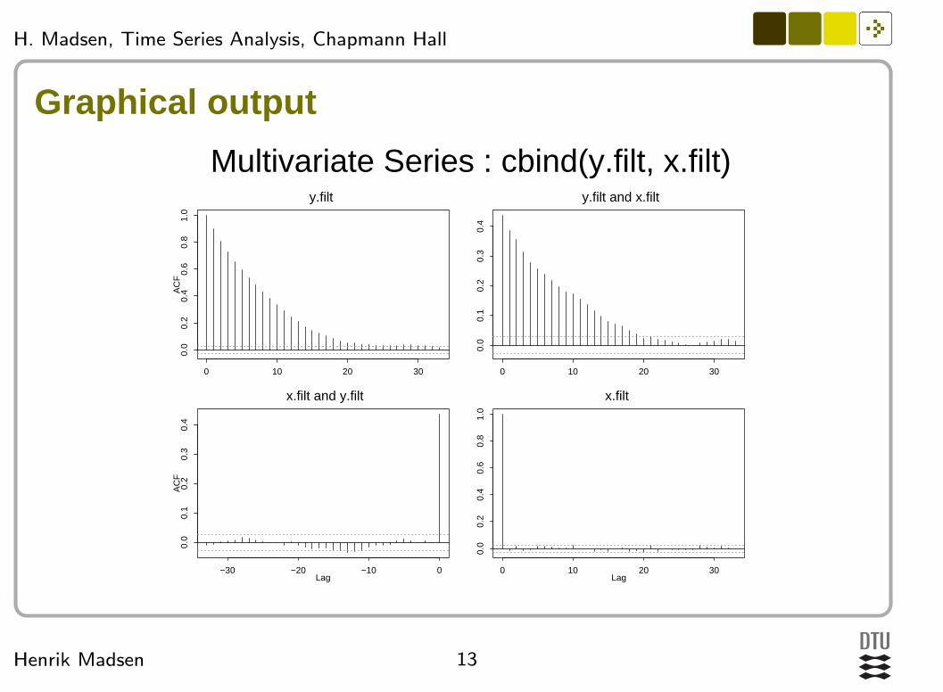
Example using S-PLUS## ARMA structure for x; AR(1)x.struct <- list(order=c(1,0,0))## Estimate the model (check for convergence):x.fit <- arima.mle(x - mean(x), model=x.struct)## Extract the model:x.mod <- x.fit$model## Filter x:x.start <- rep(mean(x), 1000)x.filt <- arima.sim(model=list(ma=x.mod$ar),
innov=x, start.innov = x.start)## Filter y:y.start <- rep(mean(y), 1000)y.filt <- arima.sim(model=list(ma=x.mod$ar),
innov=y, start.innov = y.start)## Estimate SCCF for the filtered series:acf(cbind(y.filt, x.filt))
13Henrik Madsen
H. Madsen, Time Series Analysis, Chapmann Hall
Graphical output
y.filt
AC
F
0 10 20 30
0.0
0.2
0.4
0.6
0.8
1.0
y.filt and x.filt
0 10 20 30
0.0
0.1
0.2
0.3
0.4
x.filt and y.filt
Lag
AC
F
−30 −20 −10 0
0.0
0.1
0.2
0.3
0.4
x.filt
Lag0 10 20 30
0.0
0.2
0.4
0.6
0.8
1.0
Multivariate Series : cbind(y.filt, x.filt)
14Henrik Madsen
H. Madsen, Time Series Analysis, Chapmann Hall
Systems with measurement noise
SystemXt
inputΣ
Yt
tN
output
Yt =∞∑
i=−∞
hiXt−i +Nt.
γXY (k) =
∞∑
i=−∞
hiγXX(k − i)
15Henrik Madsen
H. Madsen, Time Series Analysis, Chapmann Hall
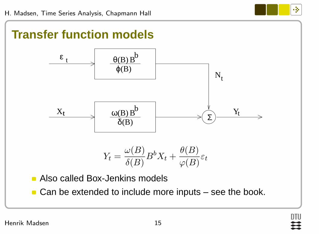
Transfer function models
Xt ΣYt
tN
bt
tε
δω
ϕθ(B)
(B)
(B)(B)
B
Bb
Yt =ω(B)
δ(B)BbXt +
θ(B)
ϕ(B)εt
Also called Box-Jenkins models
Can be extended to include more inputs – see the book.
16Henrik Madsen
H. Madsen, Time Series Analysis, Chapmann Hall
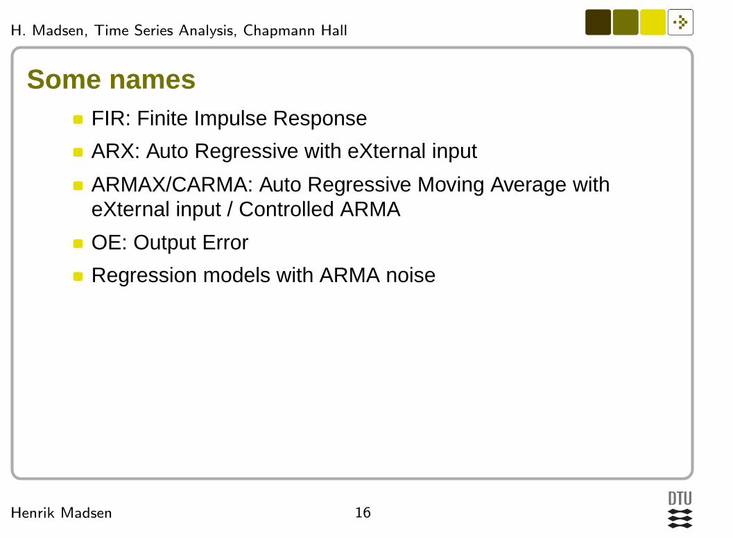
Some namesFIR: Finite Impulse Response
ARX: Auto Regressive with eXternal input
ARMAX/CARMA: Auto Regressive Moving Average witheXternal input / Controlled ARMA
OE: Output Error
Regression models with ARMA noise
17Henrik Madsen
H. Madsen, Time Series Analysis, Chapmann Hall
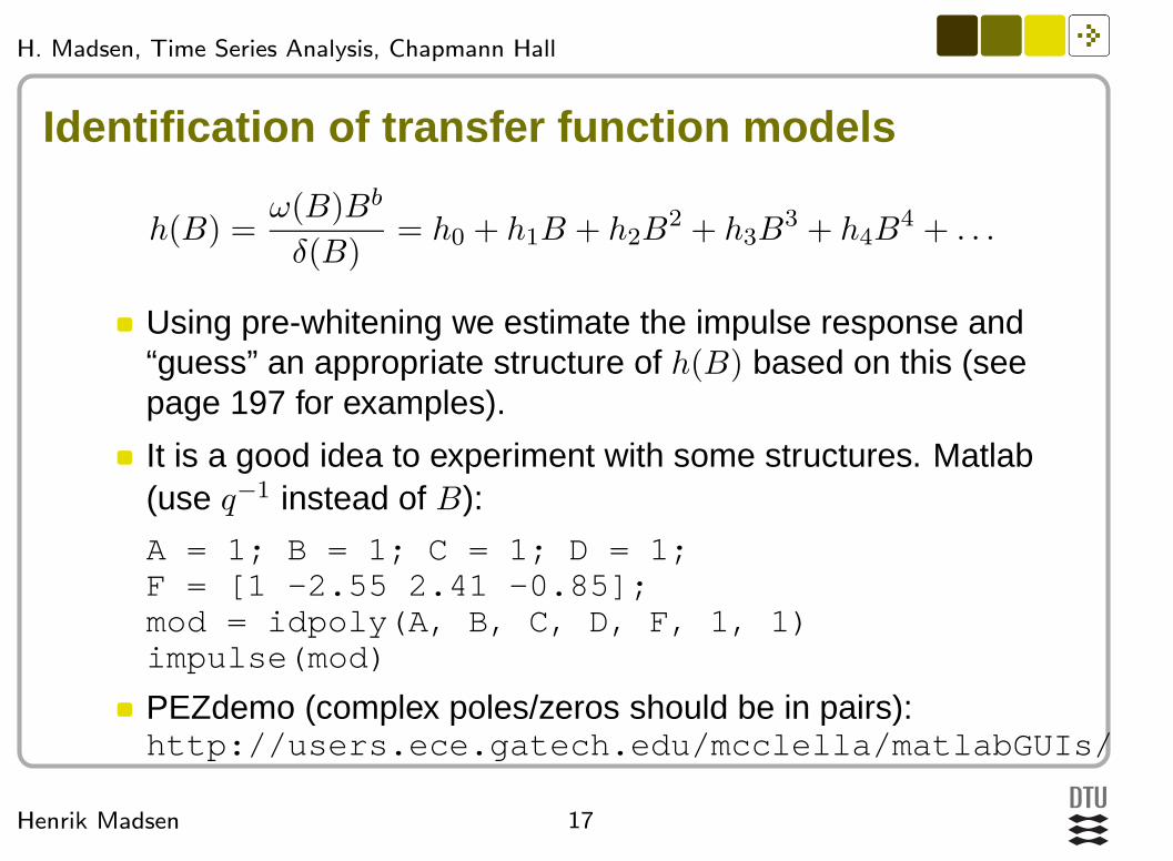
Identification of transfer function models
h(B) =ω(B)Bb
δ(B)= h0 + h1B + h2B
2 + h3B3 + h4B
4 + . . .
Using pre-whitening we estimate the impulse response and“guess” an appropriate structure of h(B) based on this (seepage 197 for examples).
It is a good idea to experiment with some structures. Matlab(use q−1 instead of B):
A = 1; B = 1; C = 1; D = 1;F = [1 -2.55 2.41 -0.85];mod = idpoly(A, B, C, D, F, 1, 1)impulse(mod)
PEZdemo (complex poles/zeros should be in pairs):http://users.ece.gatech.edu/mcclella/matlabGUIs/
18Henrik Madsen
H. Madsen, Time Series Analysis, Chapmann Hall
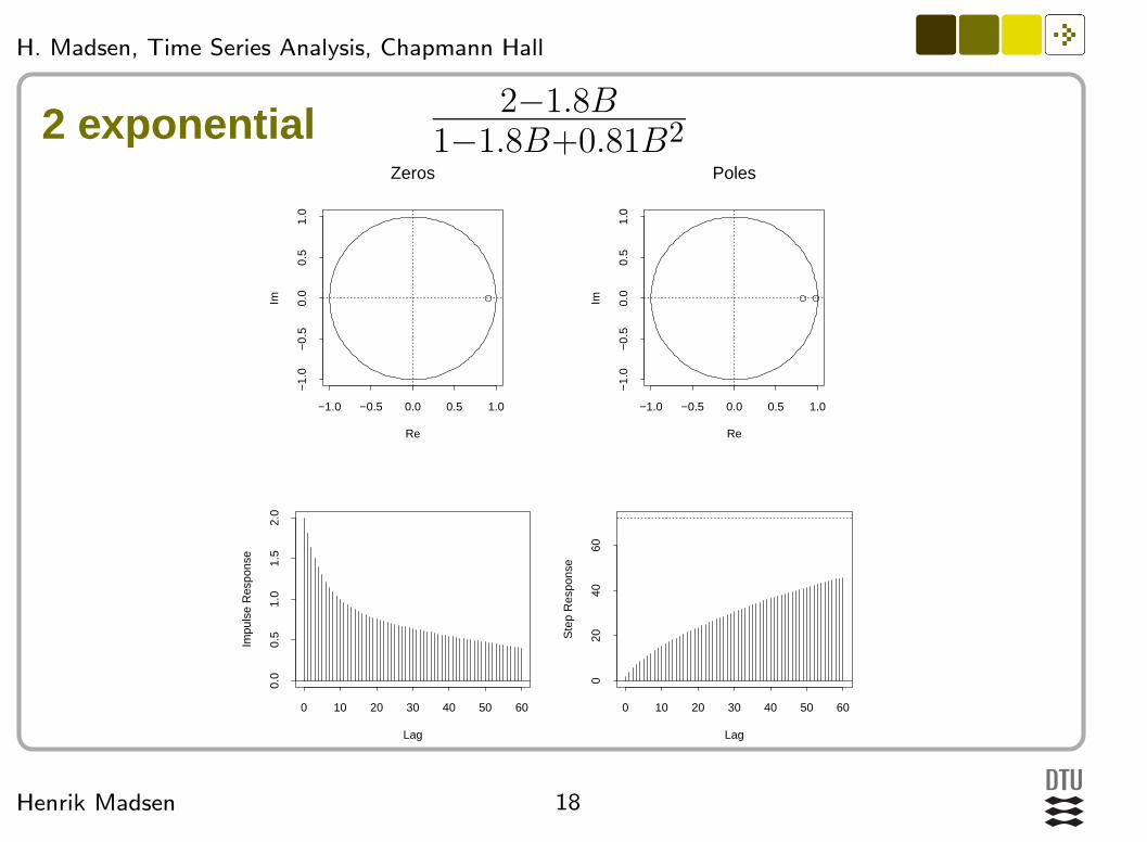
2 exponentialZeros
Re
Im
−1.0 −0.5 0.0 0.5 1.0
−1.
0−
0.5
0.0
0.5
1.0
Poles
Re
Im
−1.0 −0.5 0.0 0.5 1.0
−1.
0−
0.5
0.0
0.5
1.0
Lag
Impu
lse
Res
pons
e
0 10 20 30 40 50 60
0.0
0.5
1.0
1.5
2.0
Lag
Ste
p R
espo
nse
0 10 20 30 40 50 60
020
4060
2−1.8B
1−1.8B+0.81B2
19Henrik Madsen
H. Madsen, Time Series Analysis, Chapmann Hall
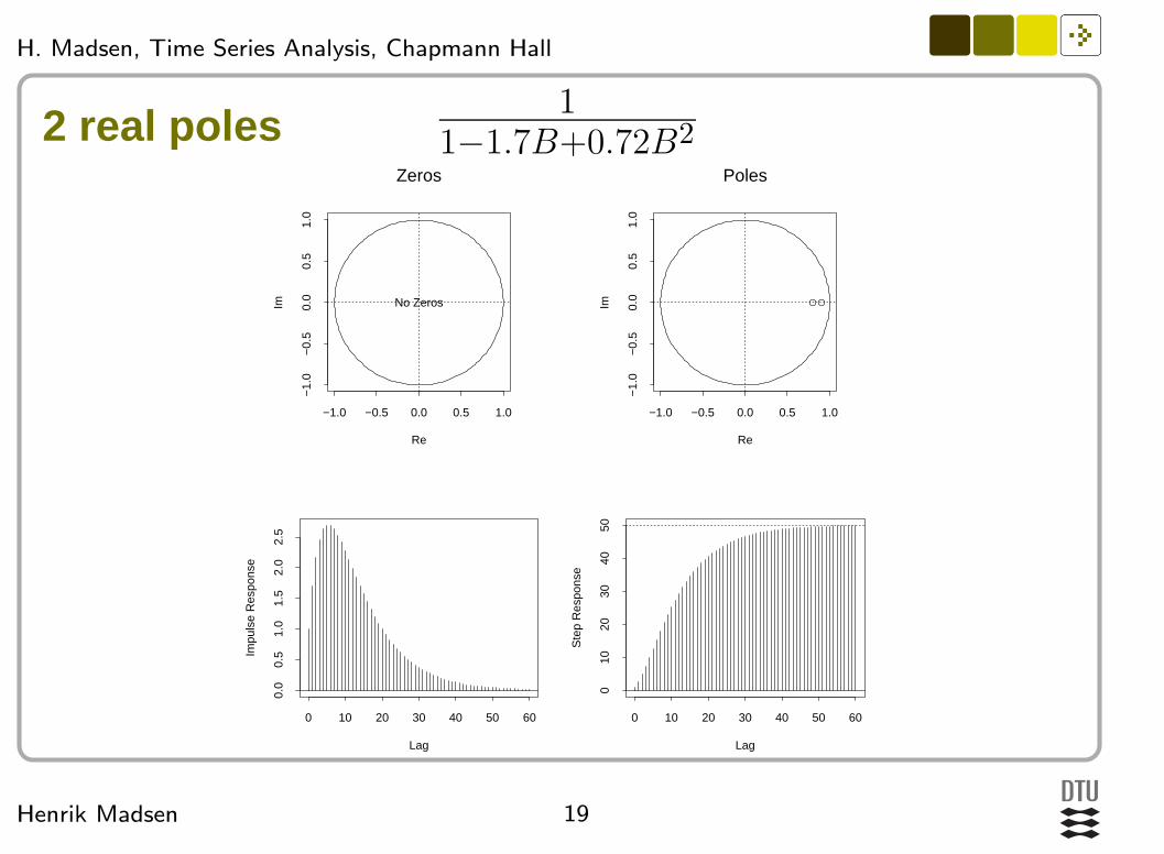
2 real polesZeros
Re
Im
−1.0 −0.5 0.0 0.5 1.0
−1.
0−
0.5
0.0
0.5
1.0
No Zeros
Poles
Re
Im
−1.0 −0.5 0.0 0.5 1.0
−1.
0−
0.5
0.0
0.5
1.0
Lag
Impu
lse
Res
pons
e
0 10 20 30 40 50 60
0.0
0.5
1.0
1.5
2.0
2.5
Lag
Ste
p R
espo
nse
0 10 20 30 40 50 60
010
2030
4050
1
1−1.7B+0.72B2

20Henrik Madsen
H. Madsen, Time Series Analysis, Chapmann Hall
2 complexZeros
Re
Im
−1.0 −0.5 0.0 0.5 1.0
−1.
0−
0.5
0.0
0.5
1.0
No Zeros
Poles
Re
Im
−1.0 −0.5 0.0 0.5 1.0
−1.
0−
0.5
0.0
0.5
1.0
Lag
Impu
lse
Res
pons
e
0 10 20 30
−0.
50.
00.
51.
01.
5
Lag
Ste
p R
espo
nse
0 10 20 30
01
23
45
1
1−1.5B+0.81B2
21Henrik Madsen
H. Madsen, Time Series Analysis, Chapmann Hall
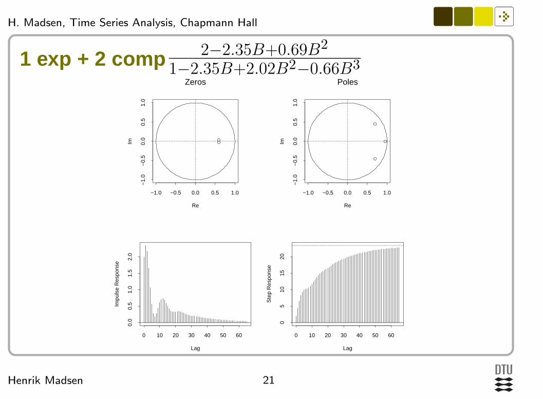
1 exp + 2 compZeros
Re
Im
−1.0 −0.5 0.0 0.5 1.0
−1.
0−
0.5
0.0
0.5
1.0
Poles
Re
Im
−1.0 −0.5 0.0 0.5 1.0
−1.
0−
0.5
0.0
0.5
1.0
Lag
Impu
lse
Res
pons
e
0 10 20 30 40 50 60
0.0
0.5
1.0
1.5
2.0
Lag
Ste
p R
espo
nse
0 10 20 30 40 50 60
05
1015
20
2−2.35B+0.69B2
1−2.35B+2.02B2−0.66B3

22Henrik Madsen
H. Madsen, Time Series Analysis, Chapmann Hall
Identification of the transfer function for the noiseAfter selection of the structure of the transfer function of theinput we estimate the parameters of the model
Yt =ω(B)
δ(B)BbXt +Nt
We extract the residuals {Nt} and identifies a structure for anARMA model of this series
Nt =θ(B)
ϕ(B)εt ⇔ ϕ(B)Nt = θ(B)εt
We then have the full structure of the model and we estimateall parameters simultaneously
23Henrik Madsen
H. Madsen, Time Series Analysis, Chapmann Hall
EstimationForm 1-step predictions, treating the input {Xt} as known inthe future (if {Xt} is really stochastic we condition on theobserved values)
Select the parameters so that the sum of squares of theseerrors is as small as possible
If {εt} is normal then the ML estimates are obtained
For FIR and ARX models we can write the model asY t = X
Tt θ + εt and use LS-estimates
Moment estimates: Based on the structure of the transferfunction we find the theoretical impulse response and wemake a match with the lowest lags in the estimated impulseresponse
Output error estimates . . .
24Henrik Madsen
H. Madsen, Time Series Analysis, Chapmann Hall
Model validationAs for ARMA models with the additions:
Test for cross correlation between the residuals and the input
ρεX(k) ∼ Norm(0, 1/N)
which is (approximately) correct when {εt} is white noise andwhen there is no correlation between the input and theresiduals
A Portmanteau test can also be performed
25Henrik Madsen
H. Madsen, Time Series Analysis, Chapmann Hall
Prediction Yt+k|t
We must consider two situations
The input is controllable, i.e. we can decide it and we canpredict under different input-scenarios. In this case theprediction error variance is originating from the ARMA-partonly (Nt).
The input is only known until the present time point t and topredict the output we must predict the input. In this case theprediction error variance depend also on the autocovariance ofthe input process. In the book the case where the input can bemodelled as an ARMA-process is considered.

26Henrik Madsen
H. Madsen, Time Series Analysis, Chapmann Hall
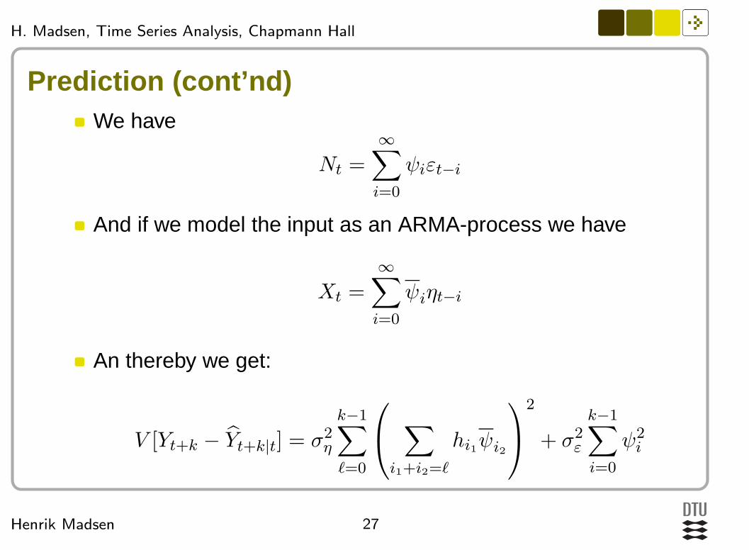
Prediction (cont’nd)
Yt+k|t =k−1∑
i=0
hiXt+k−i|t +∞∑
i=k
hiXt+k−i + Nt+k|t.
Yt+k − Yt+k|t =
k−1∑
i=0
hi(Xt+k−i − Xt+k−i|t) +Nt+k − Nt+k|t
If the input is controllable then Xt+k−i|t = Xt+k−i
The book also considers the case where output is known untiltime t and input until time t+ j
27Henrik Madsen
H. Madsen, Time Series Analysis, Chapmann Hall
Prediction (cont’nd)We have
Nt =
∞∑
i=0
ψiεt−i
And if we model the input as an ARMA-process we have
Xt =
∞∑
i=0
ψiηt−i
An thereby we get:
V [Yt+k − Yt+k|t] = σ2η
k−1∑
ℓ=0
∑
i1+i2=ℓ
hi1ψi2
2
+ σ2ε
k−1∑
i=0
ψ2i

28Henrik Madsen
H. Madsen, Time Series Analysis, Chapmann Hall
Yt =0.4
1−0.6BXt +1
1−0.4εt, σ2ε = 0.036
y x h xf N | y x h xf N
1 2.04 1.661 0.00403 2.21 -0.1645 | 2.04 1.661 0.00403 2.21 -0.1645
2 3.05 4.199 0.00672 3.00 0.0407 | 3.05 4.199 0.00672 3.00 0.0407
3 2.34 1.991 0.01120 2.60 -0.2566 | 2.34 1.991 0.01120 2.60 -0.2566
4 2.49 2.371 0.01866 2.51 -0.0186 | 2.49 2.371 0.01866 2.51 -0.0186
5 3.30 3.521 0.03110 2.91 0.3826 | 3.30 3.521 0.03110 2.91 0.3826
6 3.53 3.269 0.05184 3.06 0.4768 | 3.53 3.269 0.05184 3.06 0.4768
7 2.72 0.741 0.08640 2.13 0.5880 | 2.72 0.741 0.08640 2.13 0.5880
8 2.46 2.238 0.14400 2.17 0.2888 | 2.46 2.238 0.14400 2.17 0.2888
9 NA 2.544 0.24000 2.32 NA | 2.44 2.544 0.24000 2.32 0.1155
10 NA 3.201 0.40000 2.67 NA | 2.72 3.201 0.40000 2.67 0.0462
To forecast y (9,10) we must filter x as in xf, calc. N for the
historic data, forecast N and add that to xf (future values)
> Nfc <- arima.forecast(N[1:8], model=list(ar=0.4), sigma2=0.036, n=2)
> Nfc$mean:
[1] 0.1155 0.0462

29Henrik Madsen
H. Madsen, Time Series Analysis, Chapmann Hall
Intervention models
It =
{1 t = t00 t 6= t0
Yt =ω(B)
δ(B)It +
θ(B)
φ(B)εt
See a real life example in the book.