Tilburg University You'll Never Walk Alone Colella ... · legislation. In August 2013, as a matter...

Tilburg University

You'll Never Walk Alone

Colella, Fabrizio; Dalton, Patricio; Giusti, G.

Document version:Publisher's PDF, also known as Version of record

Publication date:2018

Link to publication

Citation for published version (APA):Colella, F., Dalton, P., & Giusti, G. (2018). You'll Never Walk Alone: The Effect of Moral Support onPerformance. (CentER Discussion Paper; Vol. 2018-026). Tilburg: CentER, Center for Economic Research.

General rightsCopyright and moral rights for the publications made accessible in the public portal are retained by the authors and/or other copyright ownersand it is a condition of accessing publications that users recognise and abide by the legal requirements associated with these rights.

- Users may download and print one copy of any publication from the public portal for the purpose of private study or research - You may not further distribute the material or use it for any profit-making activity or commercial gain - You may freely distribute the URL identifying the publication in the public portal

Take down policyIf you believe that this document breaches copyright, please contact us providing details, and we will remove access to the work immediatelyand investigate your claim.

Download date: 05. Jan. 2020

https://research.tilburguniversity.edu/en/publications/1dac53ca-9483-48f5-84b0-0ea70f06f80b

No. 2018-026

YOU’LL NEVER WALK ALONE: THE EFFECT OF MORAL SUPPORT ON PERFORMANCE

By

Fabrizio Colella, Patricio S. Dalton, Giovanni Giusti

16 July 2018

ISSN 0924-7815 ISSN 2213-9532

You’ll Never Walk Alone:

The Effect of Moral Support on Performance

Fabrizio Colella∗ Patricio S. Dalton† Giovanni Giusti‡

July 14, 2018

Abstract

This study presents evidence on the role of moral support on performance in a compet-itive environment. We take advantage of an unusual change in the Argentinean footballlegislation. In August 2013, as a matter of National security, the Argentinean govern-ment forced all the teams of the first division to play their games with only home teamsupporters. Supporters of the visiting teams were not allowed to be in stadiums duringleague games. We estimate the effect of this exogenous variation of supporters on teamperformance, and we find that visiting teams are, on average, about 20% more likely tolose without their supporters. Moreover, we find that the lack of supporters of the vis-iting team increased the score differential between the home team and the visitor. Theeffect of the ban is stronger for big teams, who have the highest number of supporterswhen playing away. In addition, we find no evidence of changes of referees’ decisions dueto the ban, suggesting that the effect on team performance is due to the loss of moralsupport rather than a change in referees hostility. As placebo test, we run the analysisusing contemporaneous cup matches, where the visiting team supporters were allowedto attend. We find no effect of the ban on the cup games, which provides additionalempirical support to our findings. Our results offer unique and novel empirical evidenceof the importance on moral support on performance.

JEL: D01, D91, J24.Keywords: Support, Encouragement, Motivation, Football, Team Performance, Non-monetary incentives, Competitive Environments

We thank Remco Geervliet for excellent research assistance. We also thank participants at the 2017Gerzensee Conference in Engelberg, the 2018 Spring Meetings of Young Economists in Palma de Mallorca,and the Labor Research Group Meeting in Lausanne. We are especially grateful to Johannes Buggle, RafaelLalive, Margaret Meyer, David Schindler and Jan Van Ours for useful comments and suggestions. The usualdisclaimer applies.∗Department of Economics, University of Lausanne; e-mail: [email protected]†Department of Economics, Tilburg University; e-mail: [email protected]‡Tecnocampus, Universitat Pompeu Fabra; e-mail: [email protected]

“Que serıa de un club sin el hincha. Una bolsa vacıa. El hincha es el alma de los colores,

es el que no se ve. Es el que da todo sin esperar nada. Eso es ser hincha. Ese soy yo.”

Enrique Santos Discepolo (Fragmento de la pelıcula “El Hincha”, 1951).

“What would be of a club without supporters? It would be an empty bag. Supporters are

the soul of the colors; they are those who are not seen. Those who give everything without

expecting nothing. That is being a supporter. That is who I am.”

Enrique Santos Discepolo (Part of the movie “El Hincha”, 1951).

1 Introduction

As humans, we spend considerable time providing moral support to others. We use pep

talks, encouraging words, and similar unverifiable soft information to boost confidence and

“motivate” others. Indeed, the use of encouragement, praise and motivation strategies is

a central theme in management, coaching, education and political marketing. Each year

billions of dollars are spent in books and counseling by people who want to be inspired

and motivated. Successful coaches are viewed as those who build up others’ confidence

(Kinlaw 1999). Even Barak Obama’s “Yes We Can” slogan has a gist of moral support on

it: to impinge a believe on his followers that an outcome that was previously thought to be

unattainable, is actually attainable now.

Why do people spend resources to morally support others? Social psychologists have

rationalized the supply of moral support with two main empirical facts. The first fact is that

self-confidence, defined as the belief to be able to succeed in a task, improves performance

(Bandura 1986). There is plenty of empirical evidence consistent with this fact within ed-

ucational, labor and competitive sports contexts (Stajkovic and Luthans (1998); Bandura

(2000); Bandura and Locke (2003)). The second fact is that self-confidence can be manipu-

lated externally. An example of this is a well-known phenomenon studied in the literature of

social-psychology coined “The Pygmalion” effect (Rosenthal and Jacobson 1968), whereby

others’ expectations about own ability to perform a task can shape self-confidence and have

an impact on performance. In economic jargon, these two facts give rise for a principal

(e.g. parent, spouse, friend, teacher, boss), who is interested in improving an agent’s per-

formance, to use moral support strategically. Indeed, Benabou and Tirole (2003) formalize

this idea in a principal-agent game theoretic model in which the agent has imperfect knowl-

edge about her own ability. The principal, who has a stake in her performance, has strong

incentives to send signals to the agent that she is of high ability. This would boost agents’

1

self-confidence, her interest in the task and consequently her performance. Moral support

is then formalized in economics as a confidence enhancement strategy of the principal.

Despite its prevalence and importance, the evidence of the causal effect of moral support

on performance is rather scarce. The major empirical challenge resides on the fact that

moral support is essentially endogenous. People strategically choose whether to supply or

demand moral support, how much of it, to whom to supply and from whom to demand.

For example, better performing people (being children, students, workers, or teams) attract

higher support (from parents, teachers, bosses or fans) and, at the same time, people who

receive more support perform better. This imposes a real challenge for identification of the

causal relationship between moral support and performance.

This paper addresses this challenge by taking advantage of an exogenous change in

moral support caused by an unexpected change of law in the Argentinean football league.

Following an incident in which a football supporter got killed, the authorities decided to

implement a drastic measure in the form of a ban (Act: 4810, 20 August, 2013) forbidding

the presence of teams visiting supporters during first division matches. Only local team

supporters could be at the stadium while the part destined to visitors remained empty.

This provides an unusually clean opportunity in a real-world environment to discern the

effect of moral support on performance.

Using data from 1320 matches played before and after the introduction of the ban, we

find that the probability for the visiting team to lose a match without their supporters

increases by about 20%. This effect is robust to different time and season fixed effects.

Moreover, we find that the lack of supporters of the visiting team increased the score

differential. The odds that the visiting team concedes an additional goal more than the

home team increases by 1.3 times with the law. The effect of the ban is stronger for big

teams, who have the highest number of supporters when playing away. In addition, we

find no evidence of changes of referees’ decisions due to the ban, suggesting that the effect

on team performance is due to the loss of moral support rather than a change in referees

hostility. As placebo test, we run the analysis using contemporaneous cup matches, where

the visitors supporters were allowed to attend. We find no effect of the ban on the cup

games, which provides additional empirical support to our findings.

We believe football provides a unique environment to study moral support. As stated by

Palacios-Huerta (2014, p. 2) “of the three ingredients that soccer offers, the most essential

to its success is neither the ball nor the players but the flag”. In football “you’ll never

walk alone” - unless it gets prohibited by law. According to Alabarces and Rodrigues

(1996), football is the major phenomenon of mass communication in the world, and one

2

of the strongest identification practices of the popular sectors in most of Latin America

countries. Supporting a particular club is a form of identity, and this is particularly strong

for Argentinean football supporters, who do not consider themselves as spectators, but as

the twelfth player. They invent hundreds of different elaborated songs to support their

teams, they jump singing these songs during the whole match, even (or specially) when

their team is losing. They move in big hordes of people, bringing their flags where the

team plays, even thousands of kilometers away, as a signal of fidelity and support to the

“colours they love”. This particular environment of social support combined with a sudden

exogenous ban, makes the Argentinean case an ideal natural experiment. To the best of our

knowledge, this paper is the first to empirically examine moral support and performance in

a highly competitive environment by using exogenous variation for this purpose.

The rest of the paper is structured as follows. Section 2 relates our paper to the existing

literature. Section 3 sketches a simple conceptual framework of the link between moral

support and performance. Section 4 introduces the institutional context and Section 5

describes the data and the empirical specification used for the analysis. Section 6 reports

the main empirical results and Section 7 concludes.

2 Related Literature

This paper contributes to several strands of literature in economics and psychology. First,

it relates to the literature highlighting the effectiveness of various forms of non-monetary

incentives on workers motivation (Deci (1971); Frey and Jegen (2001);Gneezy, Meier, and

Rey-Biel (2011)). Examples of effective non-monetary incentives are goals (Wu, Heath,

and Larrick (2008); Goerg and Kube (2012); Gomez-Minambres (2012); Corgnet, Gomez-

Minambres, and Hernan-Gonzalez (2015)), interpersonal ties (Bandiera, Barankay, and

Rasul 2010), symbolic awards (Kosfeld and Neckermann (2011), authority (Fehr, Herz,

and Wilkening (2013)) and autonomy (Falk and Kosfeld (2006)). We contribute to this

literature by showing unique evidence of the role of moral support as a novel non-monetary

incentive to increase workers performance.

Second, this paper contributes to the emerging literature that uses sport data to bring

insights into human behavior (for an excellent review, see Palacios-Huerta (2014)). Sport

data have been recently applied to the study of a variety of important problems such

as racial integration (Goff, McCormick, and Tollison 2002), competition in the workplace

(Brown 2011), national well-being (Kavetsos and Szymanski 2010), national culture on indi-

vidual violence (Miguel, Saiegh, and Satyanath 2008), favoritism and corruption (Garicano,

3

Palacios-Huerta, and Prendergast 2005) and behavioral biases (Gauriot and Page (2018);

Miller and Sanjurjo (2018)). Related to this paper, Apesteguia and Palacios-Huerta (2010)

use data on football penalty kicks to identify the effect of psychological pressure on the

probability of scoring, depending on the order of kicks.1 Feri, Innocenti, and Pin (2013)

find that the effect of psychological pressure in competitive environments is moderated by

individual differences on cognitive anxiety. Closely related to our paper, Garicano, Palacios-

Huerta, and Prendergast (2005) show that social pressure biases football referees’ toward

home teams. We show that this channel is not present in the context of our study, suggesting

that the effect of supporters on team performance is direct and not through a change of the

referees’ hostility towards visiting teams. In general, we contribute to this branch of litera-

ture by combining football data with an unusual change in a law to study an understudied

psychological factor that affects performance in a highly competitive environment.

Third, our paper is also indirectly related to the literature studying the effect of praise

and recognition on performance, as long as the presence of supporters in the stadium has

some feature of recognition too. Deci (1971) shows that providing praise increases students

willingness to work on a puzzle. More recently, in a controlled field experiment with stu-

dents, Bradler, Dur, Neckermann, and Non (2016) find that unexpected public recognition

by means of a thank-you card increases students group performance. This paper com-

plements this literature in that we study a setting with repeated interaction between the

principal (supporters) and the agent (team), during a long time span, in a very competitive

environment and where the stakes involved are substantially high.

Fourth, our paper relates, to some extent, to the psychological literature of “audience

effect”. This literature considers the mere presence of an audience as responsible for a

psychological arousal with direct impact on behavior. Zajonc (1968) finds that the perfor-

mance of cockroaches was positively affected in a simple task (finding food in a straight

maze) by the presence of an audience of cockroaches, while was negatively affected in a

complex task (finding food in a maze with several turns). A similar behavior was bound in

humans beings (Butler and Baumeister 1998). According to this literature, the effect of the

audience on individuals depends very much on the type of task and therefore performance

can be both enhanced (i.e. social support hypothesis) or impaired (i.e. social pressure hy-

pothesis). Recently, the audience effect has also began to gain attention among economists.

Filiz-Ozbay and Ozbay (2014) studied the effect of audience in a public good game finding

that if there are not strategic aspects involved in the game the result is not affected by the

audience. Charness, Rigotti, and Rustichini (2007) show that the presence of an audience

1See also Kocher, Lenz, and Sutter (2012) for a replication study.

4

affects substantially players’ choices in the Battle of Sexes game. Although supporters in

Argentine stadiums are technically considered as the audience, their role is more active than

the rather passive role of the type of audience studied in this literature.

Finally, this paper provides evidence of one understudied factor of a well-established

phenomenon in the sport economics literature: home advantage. Home advantage, refers to

a greater success rate in home versus away competitions. It is a robust phenomenon that has

been consistently highlighted in sport competition both individually (e.g. Koning (2011))

and in teams (e.g. Gomez and Pollard (2011); Liardi and Carron (2011)).2 According to

this literature, the main reasons for the existence of home advantage are: (a) influence

of the crowd, (b) familiarity with the context, (c) travel fatigue, (d) territoriality and (e)

referee bias. Related to our paper is the work of Smith and Groetzinger (2010). They

analyze the role of attendance in home-field advantage in Major League Baseball, and find

a positive association between attendance and team performance. However, their findings

suffer from endogeneity concerns. By leveraging the unique opportunity provided by the

sudden change in law, our paper identify the relative role of the supporters, fixing all the

other factors constant.

3 Framework and Hypothesis

How can moral support be conceptualized in an economic framework? In a canonical model

in which individuals respond only to monetary incentives and have perfect information about

their own ability and payoffs, moral support would not exist. Nobody would spend time

and effort trying to enhance others’ perception about their own abilities, simply because

there would be no scope to change that perception. However, in a model that allows

uncertainty about payoffs and imperfect knowledge about own ability, then moral support

can be sustained in equilibrium. This is the gist of Benabou and Tirole (2003) paper. In

their principal-agent model, the agents have imperfect knowledge about their own ability,

and engage in a costly project when they are sufficient confident about their ability to

succeed, and in the project’s net return. As a result, the principal, who has a stake in their

performance, have strong incentives to send signals to the agents that they are of good

ability. This boosts agents’ self-confidence, their interest in the task and consequently their

performance. Moral support is then formalized as a confidence enhancement strategy of the

principal.

Why would the agent believe the principal? For this to be an equilibrium outcome

2For a comprehensive review see Carron, Loughhead, and Bray (2005) and Pollard (2006).

5

the principal must have complementary private information about the task or the agents’

prospects from it. When the principal with private information makes a decision such as

encouraging the agents, it impacts agents’ willingness to perform the task as they take the

principal’s perspective in order to learn about themselves. The influence of the principal’s

decision on the agents’ behavior is then twofold: direct, through its impact on the agents’

payoff from accomplishing the task (keeping information constant), and indirect, through

the inference process. The idea is that by offering low-powered incentives, the principal

signals that she trusts the agent.

The model of Benabou and Tirole (2003) helps us understand why people spend re-

sources to provide moral support to others, and it serves as a framework to interpret the

support sport teams receive in a competitive setting. Linking the model to the context of

this study, the football players can be interpreted as the agents and the set of supporters as

the principal. The players have imperfect knowledge about their payoff from putting effort,

because they are uncertain about their own ability, or the team ability or the ability of

the other team. The supporters derive benefits from the players playing to their maximum

potential. The players play up to their potential only if they have sufficient confidence in

their own ability to succeed, and in the net return of their decisions. The supporters, with

a stake in the players’ performance, have strong incentives to manipulate signals relevant to

player’s self-knowledge, as higher self-confidence enhances players’ motivation and hence,

their performance. Supporters will want (and are willing to pay a cost) to boost players’

self-confidence, as well as their interest in winning the match. They do so by going to the

stadium and supporting the team with songs and banners. The hypothesis derived from

this framework is straightforward: teams with moral support are less likely to loose.

The framework of Benabou and Tirole (2003) may not be the only way to rationalize the

link between moral support and performance in our setting. In principle, the support in the

stadium could potentially increase visiting teams performance if, for example, it changes

the reference point of the players or players become risk seeker. These are all plausible

channels, but yet they are theoretical conjectures. The only existing formal model of moral

support and performance that we are aware of is that of Benabou and Tirole (2003). For

that reason, we motivate our research grounded on this theory without ruling out, of course,

other plausible theoretical mechanisms.

6

4 Institutional Context

Since the conception of professional football in Argentina in 1931, violence around football

games has been a constant real problem for the country. According to the NGO “Salvemos

al Futbol”, up to date, 323 people have died due to violence episodes in Argentinian foot-

ball matches. Despite the implementation of different safety measures, such as increasing

the number of police agents in games or installing security cameras in the stadiums, the

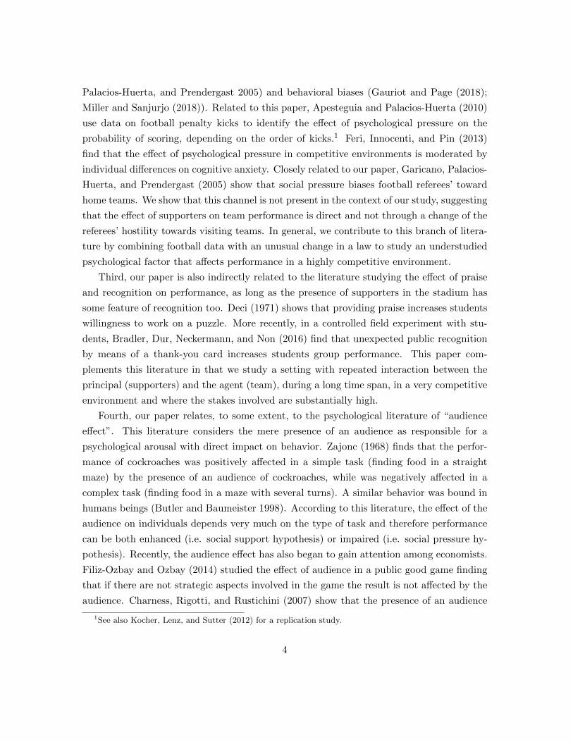
magnitude of the problem has only worsen with time. Figure 1 shows the evolution of

the number of victims in Argentinean football from the 1934 to the 2014. Excluding the

massive tragedy of 1968 during a River Plate vs. Boca Juniors match3, the overall trend

over the past century indicates an increasing number of deaths in stadiums during football

matches. Recently, the number of victims increased dramatically achieving its maximum in

the triennium 2012-2014.

Figure 1: Deaths from violence in Argentinean football

This Figure shows the number of deaths due to episodes of violence in stadiums during

professional football matches in Argentina. The database was constructed based on the

information provided by the NGO “Salvemos el futbol” and published by the newspaper

“La Nacion”

The 10th of June of 2013 marked a turning point in the history of Argentinean football.

During the match of the first division (Primera Division) between Club Atletico Lanus and

3This tragedy, known as “Tragedia de la puerta 12”, was originated by a locked exit: the pressure causedby the mass of Boca Juniors supporters trying to exit caused the death of seventy one supporters.

7

Estudiantes de La Plata, a Lanus supporter got killed by a police rubber balled shot. Follow-

ing this incident, the AFA (Asociacion de Futbol Argentino) together with the A.Pre.Vi.De

(Agencia Prevencion Violencia en el Deporte) decided to implement a drastic measure in

order to limit violence. The measure imposed was in the form of a ban forbidding the pres-

ence of visiting team supporters during first division matches (Act: 4810, 20 August, 2013).

Only local team supporters could be at the stadium while the part destined to visitors had

to remain empty. The measure is still in place at the moment, though it has been lifted by

the government in some selected matches after 2015.

5 Data and Identification Strategy

5.1 Data

To assess the impact of the ban on team performance, we collected data of Argentinean first

division matches that were played between August 2011 and December 2014. Our main web-

site of reference was www.mismarcadores.es. In total, the dataset constructed contains 1320

matches: 380 matches for each of the first three seasons (2011/2012, 2012/2013, 2013/2014)

and 180 matches for the season 2014/2015.4 For each match we recorded the final result,

the number of goals scored by each team and the number of red cards that referees held up

in front of players of each team.5 Importantly, we don’t include data after 2015 because,

since then, the government started to lift the ban in some selected matches as pilot exercises

and this would bring endogeneity to the analysis.

Table 1 presents summary statistics of the main variables of interest (Panel A) and of

ancillary variables (Panel B). For each variable, Table 1 reports its mean before and after

the ban, the mean difference, its standard error and the result of a mean comparison t-test.

The last columns show the number of matches for which each variable is observed both,

before and after the ban. Panel A gives preliminary overview of the main results of the

paper. The share of matches in which the visiting teams lose is on average greater after the

implementation of the ban, with the difference being statistically significant (p=0.06). The

score differences in favor of the home teams increased too (p=0.08), resulting mainly as a

consequences of the number of goals conceded by the visiting teams (p=0.06). Moreover,

there is no significant difference in the average number of red cards showed to players of

4In the first three seasons, teams played twice with each of the other team, whereas in the 2014/2015season called “Torneo Transicion” teams played only once against the other teams.

5In addition, we collected data on total shots, yellow cards, corners and ball possession, but we don’t usethese data for our analysis because data for those variables are not available for all the seasons before theban.

8

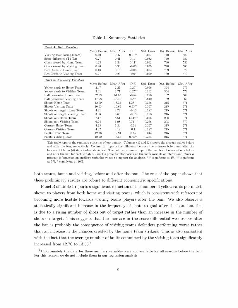
Table 1: Summary Statistics

Panel A: Main VariablesMean Before Mean After Diff. Std. Error Obs. Before Obs. After

Visiting team losing (share) 0.40 0.47 0.07∗∗ 0.027 740 580Score difference (T1-T2) 0.27 0.41 0.14∗ 0.082 740 580Goals scored by Home Team 1.23 1.34 0.11∗ 0.062 740 580Goals scored by Visiting Team 0.96 0.93 -0.03 0.055 740 580Red Cards to Home Team 0.18 0.15 -0.03 0.024 739 579Red Cards to Visiting Team 0.27 0.23 -0.04 0.029 739 579

Panel B: Ancilliary Variables

Mean Before Mean After Diff. Std. Error Obs. Before Obs. AfterYellow cards to Home Team 2.47 2.27 -0.20∗∗ 0.096 364 579Yellow cards to Visiting Team 3.01 2.77 -0.25∗∗ 0.102 364 579Ball possession Home Team 52.09 51.55 -0.54 0.796 132 569Ball possession Visiting Team 47.58 48.45 0.87 0.840 132 569Shoots Home Team 12.09 13.37 1.28∗∗∗ 0.356 215 571Shoots Visiting Team 10.03 10.66 0.63∗∗ 0.307 215 571Shoots on target Home Team 4.91 4.79 -0.13 0.182 215 571Shoots on target Visiting Team 3.86 3.68 -0.18 0.168 215 571Shoots out Home Team 7.17 8.61 1.44∗∗∗ 0.296 208 571Shoots out Visiting Team 6.24 6.98 0.74∗∗∗ 0.256 208 570Corners Home Team 4.93 5.24 0.31 0.207 215 571Corners Visiting Team 4.02 4.12 0.1 0.187 215 571Faults Home Team 12.36 12.91 0.55 0.344 215 571Faults Visiting Team 12.70 13.55 0.85∗∗ 0.355 215 571

This table reports the summary statistics of our dataset. Columns (1) and (2) report the average values beforeand after the ban, respectively. Column (3) reports the difference between the averages before and after theban and Column (4) its standard deviation. The last two columns report the number of observations beforeand after the ban for each variable. Panel A presents information on the main variable of interest and Panel Bpresents information on ancillary variables we use to support the analysis. *** significant at 1%, ** significantat 5%, * significant at 10%.

both teams, home and visiting, before and after the ban. The rest of the paper shows that

these preliminary results are robust to different econometric specifications.

Panel B of Table 1 reports a significant reduction of the number of yellow cards per match

shown to players from both home and visiting teams, which is consistent with referees not

becoming more hostile towards visiting teams players after the ban. We also observe a

statistically significant increase in the frequency of shots to goal after the ban, but this

is due to a rising number of shots out of target rather than an increase in the number of

shots on target. This suggests that the increase in the score differential we observe after

the ban is probably the consequence of visiting teams defenders performing worse rather

than an increase in the chances created by the home team strikers. This is also consistent

with the fact that the average number of faults committed by the visiting team significantly

increased from 12.70 to 13.55.6

6Unfortunately the data for these ancillary variables were not available for all seasons before the ban.For this reason, we do not include them in our regression analysis.

9

5.2 Identification Strategy

The aim of this study is to identify the effect on team performance of switching from

playing a football match as the visiting team in a stadium with both local and visiting

team supporters versus playing a football match as the visiting team in a stadium with

only local team supporters. The latent variable is overall performance of visiting teams.

As proxy for team performance we use the result of the match and the score difference,

calculated as the difference between the number of goals scored by the local team and

the goals scored by the visiting team. We estimate a Linear Probability model for the

probability of the visiting team losing a match, and an ordered Logit model for the score

difference. In both specifications, the dependent variable is regressed on a dummy variable

indicating whether the ban applies to that match or not.

Our empirical strategy essentially compares the results of the matches in the Argentinean

first league played before the ban to results of matches played after the ban was introduced.

The identification assumption relies on the non existence of other forces that could affect

the result of the matches and appear contemporaneously with the ban or in the period just

after. In other words, we assume that the expected result of every match played before the

day in which the law started to be in force and after that day would be the same if the ban

would have never been implemented.

In Section 6.6 we perform a variety of robustness checks to ensure the validity of our

results. We first conduct a placebo test using the matches from the national cup tournament

(“Copa Argentina”) instead of the league ones. The national cup is played every year

by teams from first and lower divisions of the AFA, and it fits perfectly as a placebo

experiment since the ban for visiting team supporters does not apply to the cup, plus the

games were played contemporaneously to the first division league. Second, we replicate the

main analysis dropping the matches played by teams that got promoted or relegated in

2013, and the ones played by teams that did not participate in all the four seasons. Third,

we re-run the first specification including season and round fixed effects, to control for

heterogeneity within a season, and we study the sensitivity of our results to the introduction

of time-specific fixed effects. We show that our results are robust to all these manipulations.

10

6 Results

6.1 Graphical Evidence

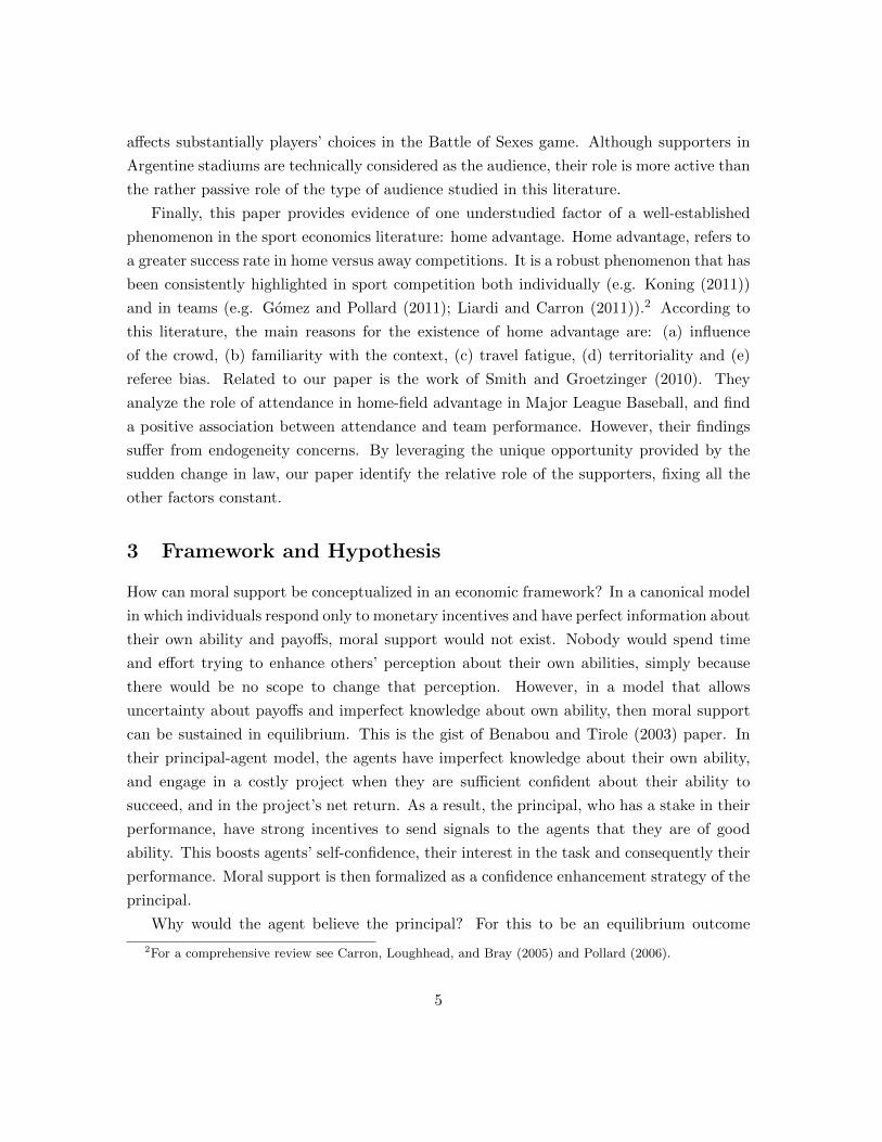
Figure 2 reports the share of matches in which the visiting teams lost by week (turn) and

its average, before and after the implementation of the ban. The evidence is based on

1,320 matches, i.e. 580 treated matches played after the implementation of the ban and 740

control matches played before. Before the ban, the probability that the away team looses a

match is around 40%.7 This probability increases to almost 47% with the ban, implying a

15.64% average increase in the probability that visiting teams lose after the ban.

Figure 2: Ratio of Matches with the Visiting Team Losing

This Figure shows the share of matches lost by visiting teams by week/turn (in dots) and its

average (the horizontal dotted lines) before and after the ban. The red vertical line represents the

date of the implementation of the law, the black vertical lines are end/beginning of each season.

7The remaining 60% is the sum of matches in which the visiting team win and draws.

11

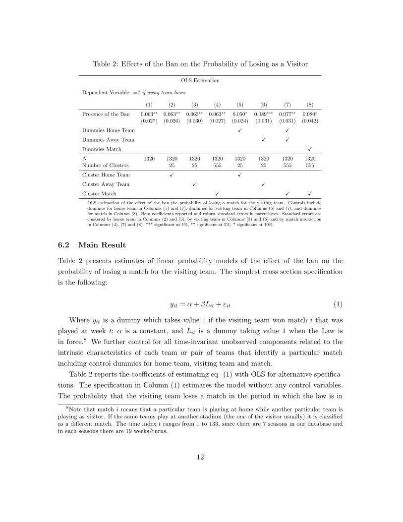
Table 2: Effects of the Ban on the Probability of Losing as a Visitor

OLS Estimation

Dependent Variable: =1 if away team loses

(1) (2) (3) (4) (5) (6) (7) (8)

Presence of the Ban 0.063∗∗ 0.063∗∗ 0.063∗∗ 0.063∗∗ 0.050∗ 0.089∗∗∗ 0.077∗∗ 0.080∗

(0.027) (0.026) (0.030) (0.027) (0.024) (0.031) (0.031) (0.042)

Dummies Home Team X X

Dummies Away Team X X

Dummies Match X

N 1320 1320 1320 1320 1320 1320 1320 1320Number of Clusters 25 25 555 25 25 555 555

Cluster Home Team X X

Cluster Away Team X X

Cluster Match X X X

OLS estimation of the effect of the ban the probability of losing a match for the visiting team. Controls includedummies for home team in Columns (5) and (7), dummies for visiting team in Columns (6) and (7), and dummiesfor match in Column (8). Beta coefficients reported and robust standard errors in parentheses. Standard errors areclustered by home team in Columns (2) and (5), by visiting team in Columns (3) and (6) and by match interactionin Columns (4), (7) and (8). *** significant at 1%, ** significant at 5%, * significant at 10%.

6.2 Main Result

Table 2 presents estimates of linear probability models of the effect of the ban on the

probability of losing a match for the visiting team. The simplest cross section specification

is the following:

yit = α+ βLit + εit (1)

Where yit is a dummy which takes value 1 if the visiting team won match i that was

played at week t; α is a constant, and Lit is a dummy taking value 1 when the Law is

in force.8 We further control for all time-invariant unobserved components related to the

intrinsic characteristics of each team or pair of teams that identify a particular match

including control dummies for home team, visiting team and match.

Table 2 reports the coefficients of estimating eq. (1) with OLS for alternative specifica-

tions. The specification in Column (1) estimates the model without any control variables.

The probability that the visiting team loses a match in the period in which the law is in

8Note that match i means that a particular team is playing at home while another particular team isplaying as visitor. If the same teams play at another stadium (the one of the visitor usually) it is classifiedas a different match. The time index t ranges from 1 to 133, since there are 7 seasons in our database andin each seasons there are 19 weeks/turns.

12

force is, on average, 6.3 percentage points greater than before, equivalent to an increase of

15.64%. Columns (2) to (4) reports OLS estimates of eq. (1) with standard errors clustered

by team or matches. This result holds also for different specifications. In the remaining

columns we add a dummy for the local team (Column 5), for the visiting team (Column

6), for both (Column 7) and for match (Column 8). In these last four specifications, the

size of the coefficient increase. Overall, Table 2 shows robust empirical evidence that the

ban increased the probability of losing a match when playing as an visiting team. Our

preferred specification is reported in Column (6), where we control for visiting team fixed

effect, because all the unobservable time invariant components related only to the visiting

team are taking into account. In this specification, the ban increases the probability of

losing a match for the visiting team by 22.1%. With this analysis we provide quantitative

evidence that the absence of teams’ supporters has a strong negative effect on the overall

performance of the team and as a consequence, in the presence of the ban, teams are more

likely to lose when playing as visitors.

Table A1 shows results from a Logit model estimating the likelihood of losing a match

for a visiting team in the presence of the ban. Again, Column (1) reports the coefficient

of the Law treatment without any additional controls. As for the linear regression model,

the presence of the ban has a positive and significant effect on the likelihood of losing a

match for the visiting team. Results do not change and remain significant at 1% level

when standard errors are clustered by home team, visiting team and matches and when

controlling for team and match fixed effect.

6.3 Score Difference

In this subsection we complement our main analysis by studying the effect of the ban on

another proxy of relative team performance: the difference between the number of goals

scored by the home team and the number of goals scored by the visiting team. We refer

to this measure as “score difference”. The specification that we use is exactly the same as

in equation (1), with the difference that as dependent variable we use the score difference

instead of a dummy for visiting team losing. Table 3 reports the estimated exponential

coefficients of an Ordered Logit model on the effect of the ban on the score difference. As

before, our preferred specification is in Column (6) where dummies for the visiting team are

included. We find that the odds that the visiting team concedes an additional goal more

than the opponent are 1.3 times greater after the ban.

In the Appendix (Table A2) we analyze the effect of the ban on the absolute number of

goals scored by each team separately. Concerning the number of goals scored by the local

13

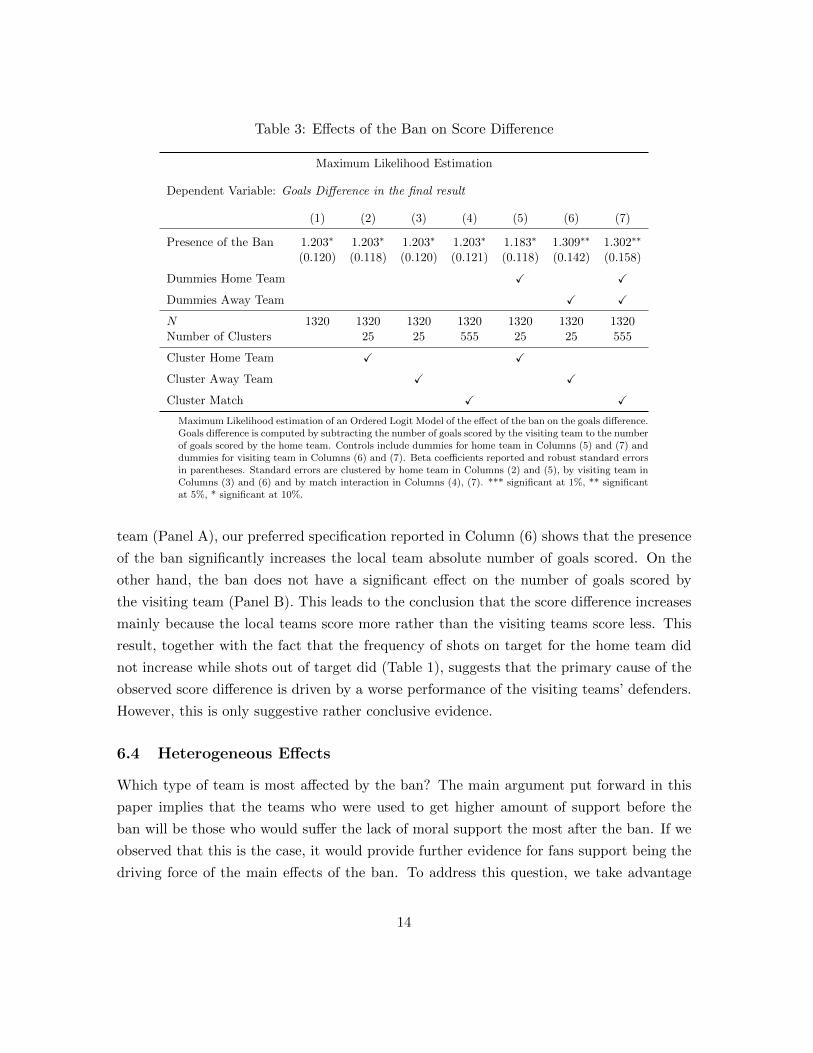
Table 3: Effects of the Ban on Score Difference

Maximum Likelihood Estimation

Dependent Variable: Goals Difference in the final result

(1) (2) (3) (4) (5) (6) (7)

Presence of the Ban 1.203∗ 1.203∗ 1.203∗ 1.203∗ 1.183∗ 1.309∗∗ 1.302∗∗

(0.120) (0.118) (0.120) (0.121) (0.118) (0.142) (0.158)



N 1320 1320 1320 1320 1320 1320 1320Number of Clusters 25 25 555 25 25 555



Cluster Match X X

Maximum Likelihood estimation of an Ordered Logit Model of the effect of the ban on the goals difference.Goals difference is computed by subtracting the number of goals scored by the visiting team to the numberof goals scored by the home team. Controls include dummies for home team in Columns (5) and (7) anddummies for visiting team in Columns (6) and (7). Beta coefficients reported and robust standard errorsin parentheses. Standard errors are clustered by home team in Columns (2) and (5), by visiting team inColumns (3) and (6) and by match interaction in Columns (4), (7). *** significant at 1%, ** significantat 5%, * significant at 10%.

team (Panel A), our preferred specification reported in Column (6) shows that the presence

of the ban significantly increases the local team absolute number of goals scored. On the

other hand, the ban does not have a significant effect on the number of goals scored by

the visiting team (Panel B). This leads to the conclusion that the score difference increases

mainly because the local teams score more rather than the visiting teams score less. This

result, together with the fact that the frequency of shots on target for the home team did

not increase while shots out of target did (Table 1), suggests that the primary cause of the

observed score difference is driven by a worse performance of the visiting teams’ defenders.

However, this is only suggestive rather conclusive evidence.

6.4 Heterogeneous Effects

Which type of team is most affected by the ban? The main argument put forward in this

paper implies that the teams who were used to get higher amount of support before the

ban will be those who would suffer the lack of moral support the most after the ban. If we

observed that this is the case, it would provide further evidence for fans support being the

driving force of the main effects of the ban. To address this question, we take advantage

14

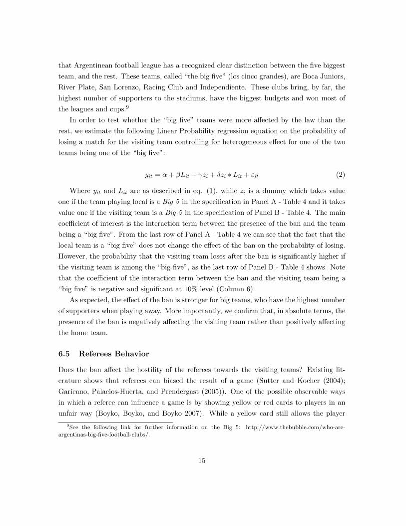
that Argentinean football league has a recognized clear distinction between the five biggest

team, and the rest. These teams, called “the big five” (los cinco grandes), are Boca Juniors,

River Plate, San Lorenzo, Racing Club and Independiente. These clubs bring, by far, the

highest number of supporters to the stadiums, have the biggest budgets and won most of

the leagues and cups.9

In order to test whether the “big five” teams were more affected by the law than the

rest, we estimate the following Linear Probability regression equation on the probability of

losing a match for the visiting team controlling for heterogeneous effect for one of the two

teams being one of the “big five”:

yit = α+ βLit + γzi + δzi ∗ Lit + εit (2)

Where yit and Lit are as described in eq. (1), while zi is a dummy which takes value

one if the team playing local is a Big 5 in the specification in Panel A - Table 4 and it takes

value one if the visiting team is a Big 5 in the specification of Panel B - Table 4. The main

coefficient of interest is the interaction term between the presence of the ban and the team

being a “big five”. From the last row of Panel A - Table 4 we can see that the fact that the

local team is a “big five” does not change the effect of the ban on the probability of losing.

However, the probability that the visiting team loses after the ban is significantly higher if

the visiting team is among the “big five”, as the last row of Panel B - Table 4 shows. Note

that the coefficient of the interaction term between the ban and the visiting team being a

“big five” is negative and significant at 10% level (Column 6).

As expected, the effect of the ban is stronger for big teams, who have the highest number

of supporters when playing away. More importantly, we confirm that, in absolute terms, the

presence of the ban is negatively affecting the visiting team rather than positively affecting

the home team.

6.5 Referees Behavior

Does the ban affect the hostility of the referees towards the visiting teams? Existing lit-

erature shows that referees can biased the result of a game (Sutter and Kocher (2004);

Garicano, Palacios-Huerta, and Prendergast (2005)). One of the possible observable ways

in which a referee can influence a game is by showing yellow or red cards to players in an

unfair way (Boyko, Boyko, and Boyko 2007). While a yellow card still allows the player

9See the following link for further information on the Big 5: http://www.thebubble.com/who-are-argentinas-big-five-football-clubs/.

15

Table 4: Heterogeneous Effects

OLS Estimation


(1) (2) (3) (4) (5) (6) (7)Panel A

Presence of the Ban 0.049 0.049∗ 0.049 0.049 0.037 0.076∗∗ 0.065∗

(0.031) (0.028) (0.033) (0.030) (0.027) (0.033) (0.034)

Local team is a big 5 0.056 0.056 0.056 0.056 0.083∗∗∗ 0.055 0.074(0.044) (0.045) (0.050) (0.043) (0.025) (0.049) (0.078)

Local team big 5 * Ban 0.064 0.064 0.064 0.064 0.056 0.056 0.047(0.066) (0.065) (0.074) (0.070) (0.058) (0.073) (0.072)

Panel B

Presence of the Ban 0.082∗∗∗ 0.082∗∗ 0.082∗∗ 0.082∗∗∗ 0.069∗∗ 0.111∗∗∗ 0.100∗∗∗

(0.031) (0.030) (0.035) (0.031) (0.029) (0.038) (0.035)

Visiting team is a big 5 -0.045 -0.045 -0.045 -0.045 -0.043 -0.173∗∗∗ -0.166∗∗

(0.043) (0.028) (0.049) (0.040) (0.028) (0.018) (0.078)

Visiting team big 5 * Ban -0.089 -0.089∗ -0.089 -0.089 -0.089 -0.096∗ -0.096(0.065) (0.052) (0.052) (0.065) (0.052) (0.047) (0.068)






Cluster Match X X

Panel A: OLS estimation of the effect of the ban the probability of losing a match for the visiting team controllingfor the local team being among the best five teams in the league. Panel B: OLS estimation of the effect of the banthe probability of losing a match for the visiting team controlling for the visiting team being among the best fiveteams in the league. Controls include dummies for home team in Columns (5) and (7) and dummies for visiting teamin Columns (6) and (7). Beta coefficients reported and robust standard errors in parentheses. Standard errors areclustered by home team in Columns (2) and (5), by visiting team in Columns (3) and (6) and by match interactionin Columns (4), (7). *** significant at 1%, ** significant at 5%, * significant at 10%.

16

Table 5: Effect of the ban on Red Cards

OLS Estimation

(1) (2) (3) (4) (5) (6) (7) (8)Panel A

Dependent Variable: Number of red cards shown to local team player

Presence of the Ban -0.029 -0.029 -0.029 -0.029 -0.037 -0.035 -0.042 -0.045(0.024) (0.024) (0.026) (0.023) (0.022) (0.029) (0.026) (0.034)

Panel B

Dependent Variable: Number of red cards shown to visiting team player

Presence of the Ban -0.044 -0.044 -0.044 -0.044 -0.042 -0.029 -0.029 -0.035(0.029) (0.027) (0.027) (0.029) (0.030) (0.028) (0.033) (0.046)

Controls



Dummies Match X




Cluster Match X X X

Panel A: OLS estimation of the effect of the ban on the number of red cards shown to local team players. Panel B:OLS estimation of the effect of the ban on the number of red cards shown to visiting team players. Controls includedummies for home team in Columns (5) and (7), dummies for visiting team in Columns (6) and (7), and dummiesfor match in Column (8). Beta coefficients reported and robust standard errors in parentheses. Standard errors areclustered by home team in Columns (2) and (5), by visiting team in Columns (3) and (6) and by match interactionin Columns (4), (7) and (8). *** significant at 1%, ** significant at 5%, * significant at 10%.

to stay in the game, a red one has a consequence that the player is immediately expelled

from the game.10 The lack of visiting supporters could in principle make the referees more

hostile towards the visiting team players. We test this conjecture by estimating eq. (1)

using as outcome variable the number of red cards shown by the referees in the matches in

our sample. Table 5 reports the results of an OLS estimation. Panel A presents the analysis

for red cards shown to the local team players and Panel B the red cards shown to the away

teams. On average the number of red cards went from 0.18 in a match before the ban, to

0.15, after the ban for home teams and from 0.27 in a match before the ban, to 0.23, after

the ban for visiting teams. Column (6) shows no significant change with respect to the

10The referee disposes of several other instruments to affect the result (e.g. adding extra time, increasingthe number of penalties). Unfortunately, we do not have access to these data over the period of analysis ofthis study.

17

number of red cards after ban with for both visiting and home teams. This result confirms

that there is no evidence of a change in referee behavior due to the ban, which supports the

hypothesis that the effect on team performance is due to the loss of moral support rather

than a change in referees hostility.

6.6 Robustness Checks

As discussed in Section 5.2, our identification strategy relies on the assumption that the

presence of the ban is orthogonal to determinants of team performance at the match-week

level. In this sub-section we perform three robustness checks which reinforce the internal

validity of our main result.

6.6.1 Counterfactual Experiment

The ideal counterfactual group for our empirical analysis would be one in which the same

teams play contemporaneously to the period we use for the analysis but in a context in

which the ban is not in place. Fortunately, the Argentine setting provides such an ideal

counterfactual. We exploit the fact that the AFA did not implement the ban for matches

played in the contemporaneous tournament “Copa Argentina”.11 This constitutes the per-

fect counterfactual, as they were games played at the same time span of the League, by

the same teams of the League but with the away supporters being allowed to attend the

stadiums. To test whether the ban had an effect on the probability of losing a match as a

visiting team, we estimate eq. (1) using matches played for the “Copa Argentina” instead

of matches played in the League. Table A3 presents the results. The coefficient of the OLS

estimation for the usual specification, reported in Column (6) is not statistically significant.

This provides further support for the fact that it is the lack of supporters that worsen vis-

iting teams performance, instead of being some unobserved factor contemporaneous to the

ban.

6.6.2 Excluding Promoted and Relegated Teams

The implementation of the ban started two weeks before the end of the season 2012/2013

and the beginning of the season 2013/2014. As mentioned in Section 5, there have been no

changes in the league structure or in the rules from one season to another. However, three

teams, Independiente, Union de Santa Fe and San Martın de Tucuman, got relegated to

the second division while three other teams, Olimpo de Bahıa Blanca, GELP and Rosario

11The “Copa Argentina” started in 2011, although other two editions were played in 1969 and 1970.

18

Central, got promoted to the first division. These two groups of teams may differ in ways

that are correlated with our dependent variable. Indeed, they do differ in the geographical

position of their stadium and the average number of visiting supporters. To account for

this concern, on top of including team fixed effects, we run as a robustness check the main

specification excluding all matches played by these six teams. As shown in table A4, our

main results remain robust to this specification.

As an extra robustness check, we perform the same analysis excluding all teams that got

promoted or relegated at least once in the study time span, restricting the sample to the

twelve teams that participated in all the seasons.12. Again, as Table A5 shows, our results

are robust to this analysis.

6.6.3 Time Fixed Effects

It is well known that football teams do not play every game at the same level. In particular,

if a team has to play several matches in short amount of time, players may put less effort in

some “less important” games, or coaches may reserve some players for particular matches.

The time of the season with higher frequency of games is not random, and the number

of matches the teams play (being league matches, national cup or continental cup) is not

random either. Usually, good teams play high frequency of games in the beginning of the

season, and only the best teams keep the same frequency until the end. Since the ban does

not apply to non-league matches, coaches may have decided to change the distribution of

energy between home matches and away matches among league, national cup, continental

cup, and this could become a confounding factor threatening our identification strategy.

In order to test whether our results are robust to a possible change in the coach strat-

egy for visiting teams within a season, we run two additional robustness checks. First

we estimate our main specification with half-season fixed effects (apertura/clausura) and

turn/week fixed effects (from 1 to 19). In this way every single turn/week within a season

is compared to the correspondent week/turn in other seasons. In a second regression, we

add month fixed effects (from 1 to 12) to compare all matches played in a particular month

of the year. Tables A6 and A7 report results of this analysis. As it can be seen, all the

coefficients of interest remain significant and the magnitude of the effect is approximately

the same as in the basic model of Table 2 for the first specification while increases by 1

percent in the second model. These results rule out any potential change of visiting teams

performance that could have happened due to time, other than the ban, confirming the

12The teams in the restricted sample are: Arsenal Sarandi, Atletico Rafaela, Belgrano, Boca Juniors,Estudiantes, Godoy Cruz, Lanus, Newell’s, Racing Club, San Lorenzo, Tigre, Velez

19

validity of our identification strategy.

7 Concluding Remarks

To the best of our knowledge, this paper provides the first empirical evidence on the effect

of moral support on performance in a natural competitive environment. Our identifica-

tion strategy takes advantage of an unusual change in the Argentinean football legislation

occurred in August 2013, which prohibited supporters to be present at the stadium when

their teams play away. We find that a sudden and unexpected lack of in-stadium support

increases, in average, 20% the probability that the visiting team looses and increases the

odds that the visiting team concedes an additional goal more than the home team by 1.3

times. Furthermore, we show that the effect of the ban is stronger for the biggest teams,

who were used to have high number of visiting supporters before the ban. In addition, we

find no evidence of changes of referees’ decisions due to the ban, suggesting that the effect

on team performance is due to the loss of moral support rather than a change in referees

hostility. As placebo test, we run the analysis using contemporaneous cup matches, where

the visiting team supporters were allowed to attend. We find no effect of the ban on the

cup games, which provides additional empirical support to our findings. Our results are

robust to a set of alternative specifications.

These findings are novel, and as such, they open new avenues for future research on

the effect of moral support on individual and team performance. The research topic is

only nascent. Laboratory and field experiments can be designed to study whether the

effect of moral support varies with the context, with the degree of competitiveness of the

environment, with the way moral support is provided or with who provides it. It would be

also interesting to study gender differences on the effect of moral support on performance,

and whether the effects are different depending on whether the agent receiving support is an

individual or a team. Finally, it would be interesting to test whether the effects we find in

the Argentinean football context can be replicated in other contexts, by using other sources

of naturally occurring exogenous shocks on moral support, such us weather conditions or

transport strikes.

20

References

Alabarces, P., and M. Rodrigues (1996): “Cuestion de Pelotas: Futbol, Deporte,Sociedad,” Cultura.

Apesteguia, J., and I. Palacios-Huerta (2010): “Psychological Pressure in Competi-tive Environments: Evidence From a Randomized Natural Experiment.,” American Eco-nomic Review, 100(5), 2548 –2564.

Bandiera, O., I. Barankay, and I. Rasul (2010): “Social incentives in the workplace,”The Review of Economic Studies, 77(2), 417–458.

Bandura, A. (1986): “The explanatory and predictive scope of self-efficacy theory,” Jour-nal of social and clinical psychology, 4(3), 359–373.

(2000): “Exercise of human agency through collective efficacy,” Current directionsin psychological science, 9(3), 75–78.

Bandura, A., and E. A. Locke (2003): “Negative self-efficacy and goal effects revisited.,”Journal of applied psychology, 88(1), 87.

Benabou, R., and J. Tirole (2003): “Intrinsic and extrinsic motivation,” The review ofeconomic studies, 70(3), 489–520.

Boyko, R. H., A. R. Boyko, and M. G. Boyko (2007): “Referee bias contributesto home advantage in English Premiership football,” Journal of sports sciences, 25(11),1185–1194.

Bradler, C., R. Dur, S. Neckermann, and A. Non (2016): “Employee recognitionand performance: A field experiment,” Management Science, 62(11), 3085–3099.

Brown, J. (2011): “Quitters never win: The (adverse) incentive effects of competing withsuperstars,” Journal of Political Economy, 119(5), 982–1013.

Butler, J. L., and R. F. Baumeister (1998): “The trouble with friendly faces: skilledperformance with a supportive audience.,” Journal of personality and social psychology,75(5), 1213.

Carron, A. V., T. M. Loughhead, and S. R. Bray (2005): “The home advantagein sport competitions: Courneya and Carron’s (1992) conceptual framework a decadelater,” Journal of sports sciences, 23(4), 395–407.

Charness, G., L. Rigotti, and A. Rustichini (2007): “Individual behavior and groupmembership,” The American Economic Review, 97(4), 1340–1352.

Corgnet, B., J. Gomez-Minambres, and R. Hernan-Gonzalez (2015): “Goal settingand monetary incentives: When large stakes are not enough,” Management Science,61(12), 2926–2944.

21

Deci, E. L. (1971): “Effects of externally mediated rewards on intrinsic motivation.,”Journal of personality and Social Psychology, 18(1), 105.

Falk, A., and M. Kosfeld (2006): “The hidden costs of control,” American EconomicReview, 96(5), 1611–1630.

Fehr, E., H. Herz, and T. Wilkening (2013): “The lure of authority: Motivation andincentive effects of power,” American Economic Review, 103(4), 1325–59.

Feri, F., A. Innocenti, and P. Pin (2013): “Is there psychological pressure in competi-tive environments?,” Journal of Economic Psychology, 39, 249–256.

Filiz-Ozbay, E., and E. Y. Ozbay (2014): “Effect of an audience in public goods provi-sion,” Experimental Economics, 17(2), 200–214.

Frey, B. S., and R. Jegen (2001): “Motivation crowding theory,” Journal of economicsurveys, 15(5), 589–611.

Garicano, L., I. Palacios-Huerta, and C. Prendergast (2005): “Favoritism undersocial pressure,” The Review of Economics and Statistics, 87(2), 208–216.

Gauriot, R., and L. Page (2018): “Fooled by performance randomness: over-rewardingluck,” The Review of Economics and Statistics, forthcoming.

Gneezy, U., S. Meier, and P. Rey-Biel (2011): “When and why incentives (don’t)work to modify behavior,” The Journal of Economic Perspectives, 25(4), 191–209.

Goerg, S., and S. Kube (2012): “Goals (th) at Work–Goals, Monetary Incentives, andWorkers Performance,” Unpublished manuscript.

Goff, B. L., R. E. McCormick, and R. D. Tollison (2002): “Racial integration as aninnovation: Empirical evidence from sports leagues,” American Economic Review, 92(1),16–26.

Gomez, M. A., and R. Pollard (2011): “Reduced home advantage for basketball teamsfrom capital cities in Europe,” European Journal of Sport Science, 11(2), 143–148.

Gomez-Minambres, J. (2012): “Motivation through goal setting,” Journal of EconomicPsychology, 33(6), 1223–1239.

Kavetsos, G., and S. Szymanski (2010): “National well-being and international sportsevents,” Journal of Economic Psychology, 31(2), 158–171.

Kinlaw, D. C. (1999): Coaching for commitment: Interpersonal strategies for obtainingsuperior performance from individuals and teams. Jossey-Bass/Pfeiffer.

Kocher, M. G., M. V. Lenz, and M. Sutter (2012): “Psychological pressure in compet-itive environments: New evidence from randomized natural experiments,” ManagementScience, 58(8), 1585–1591.

22

Koning, R. H. (2011): “Home advantage in professional tennis,” Journal of Sports Sci-ences, 29(1), 19–27.

Kosfeld, M., and S. Neckermann (2011): “Getting more work for nothing? Symbolicawards and worker performance,” American Economic Journal: Microeconomics, 3(3),86–99.

Liardi, V. L., and A. V. Carron (2011): “An analysis of National Hockey League face-offs: Implications for the home advantage,” International Journal of Sport and ExercisePsychology, 9(2), 102–109.

Miguel, E., S. M. Saiegh, and S. Satyanath (2008): “National Cultures and SoccerViolence,” NBER Working Papers 13968, National Bureau of Economic Research, Inc.

Miller, J. B., and A. Sanjurjo (2018): “Surprised by the hot hand fallacy? A truth inthe law of small numbers,” Econometrica, forthcoming.

Palacios-Huerta, I. (2014): Beautiful game theory: How soccer can help economics.Princeton University Press.

Pollard, R. (2006): “Home advantage in soccer: variations in its magnitude and a liter-ature review of the inter-related factors associated with its existence,” Journal of SportBehavior, 29(2), 169.

Rosenthal, R., and L. Jacobson (1968): “Pygmalion in the classroom,” The urbanreview, 3(1), 16–20.

Smith, E. E., and J. D. Groetzinger (2010): “Do fans matter? The effect of attendanceon the outcomes of major league baseball games,” Journal of Quantitative Analysis inSports, 1(6).

Stajkovic, A. D., and F. Luthans (1998): “Self-efficacy and work-related performance:A meta-analysis.,” Psychological bulletin, 124(2), 240.

Sutter, M., and M. G. Kocher (2004): “Favoritism of agentsthe case of referees’ homebias,” Journal of Economic Psychology, 25(4), 461–469.

Wu, G., C. Heath, and R. Larrick (2008): “A prospect theory model of goal behavior,”Unpublished manuscript.

Zajonc, R. B. (1968): “Attitudinal effects of mere exposure,” Journal of Personality andSocial Psychology, 9(2 Part 2), 1–27.

23

Appendix

Logit

Table A1: Logit



(1) (2) (3) (4) (5) (6) (7) (8)

Presence of the Ban (d) 0.063∗∗ 0.063∗∗ 0.063∗∗ 0.063∗∗ 0.032∗∗ 0.094∗∗∗ 0.064∗∗ 0.105∗∗

(0.027) (0.026) (0.030) (0.027) (0.016) (0.032) (0.031) (0.041)



Dummies Match X




Cluster Match X X X

Maximum likelihood estimation of a logit model of the effect of the ban the probability of losing a match for the visitingteam. Controls include dummies for home team in Columns (5) and (7), dummies for visiting team in Columns (6)and (7), and dummies for match in Column (8). Beta coefficients reported and robust standard errors in parentheses.Standard errors are clustered by home team in Columns (2) and (5), by visiting team in Columns (3) and (6) and bymatch interaction in Columns (4), (7) and (8). *** significant at 1%, ** significant at 5%, * significant at 10%.

24

Goals Scored

Table A2: Effect of the ban on Goals Scored


(1) (2) (3) (4) (5) (6) (7)Panel A

Dependent Variable: Number of goals scored by the local team

Presence of the Ban 1.195∗ 1.195∗∗ 1.195 1.195∗ 1.152 1.302∗∗ 1.265∗

(0.120) (0.109) (0.147) (0.119) (0.112) (0.172) (0.152)

Panel B

Dependent Variable: Number of goals scored by the visiting team

Presence of the Ban 0.944 0.944 0.944 0.944 0.940 0.901 0.894(0.0965) (0.103) (0.110) (0.0955) (0.114) (0.127) (0.112)

Controls






Cluster Match X X

]Panel A: Maximum Likelihood estimation of an ordered Logit Model of the effect of the ban on the numberof goals scored by the local team. Panel B:Maximum Likelihood Estimation of an ordered Logit Model ofthe effect of the ban on the number of goals scored by the visiting team. Controls include dummies forhome team in Columns (5) and (7) and dummies for visiting team in Columns (6) and (7). Beta coefficientsreported and robust standard errors in parentheses. Standard errors are clustered by home team in Columns(2) and (5), by visiting team in Columns (3) and (6) and by match interaction in Columns (4), (7). ***significant at 1%, ** significant at 5%, * significant at 10%.

25

Robustness

National Cup Placebo Test

Table A3: Main Regression using Cup Matches

OLS Estimation


(1) (2) (3) (4) (5) (6) (7)

Presence of the Ban 0.038 0.038 0.038 0.038 -0.038 0.123 0.202(0.083) (0.080) (0.083) (0.084) (0.112) (0.135) (0.254)






Cluster Match X X

OLS estimation of the effect of the ban on the probability of losing a match for the visiting team. Sample:all matches of the Copa Argentina between August 2011 and December 2015. Controls include dummiesfor home team in Columns (5) and (7) and dummies for visiting team in Columns (6) and (7). Betacoefficients reported and robust standard errors in parentheses. Standard errors are clustered by hometeam in Columns (2) and (5), by visiting team in Columns (3) and (6) and by match interaction inColumns (4), (7). *** significant at 1%, ** significant at 5%, * significant at 10%.

26

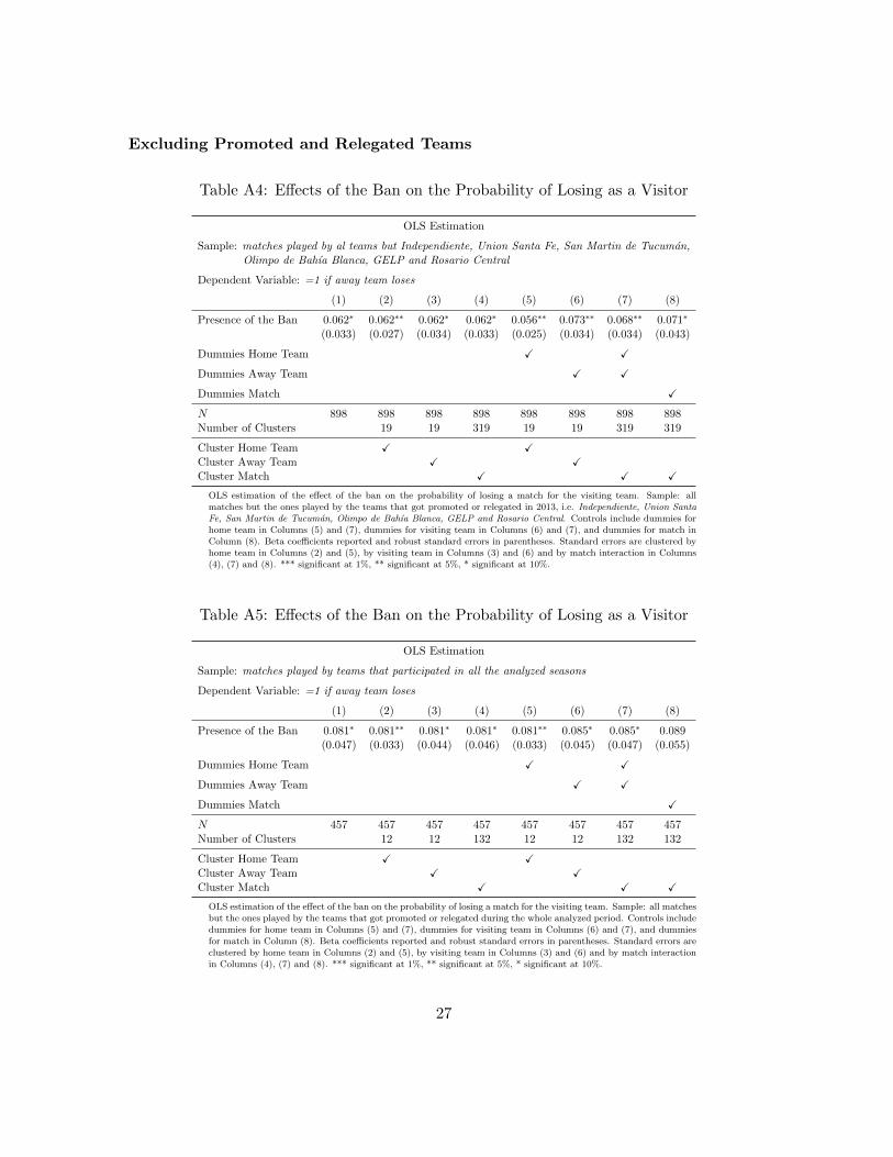
Excluding Promoted and Relegated Teams

Table A4: Effects of the Ban on the Probability of Losing as a Visitor

OLS Estimation

Sample: matches played by al teams but Independiente, Union Santa Fe, San Martin de Tucuman,Olimpo de Bahıa Blanca, GELP and Rosario Central


(1) (2) (3) (4) (5) (6) (7) (8)

Presence of the Ban 0.062∗ 0.062∗∗ 0.062∗ 0.062∗ 0.056∗∗ 0.073∗∗ 0.068∗∗ 0.071∗

(0.033) (0.027) (0.034) (0.033) (0.025) (0.034) (0.034) (0.043)



Dummies Match X


Cluster Home Team X XCluster Away Team X XCluster Match X X X

OLS estimation of the effect of the ban on the probability of losing a match for the visiting team. Sample: allmatches but the ones played by the teams that got promoted or relegated in 2013, i.e. Independiente, Union SantaFe, San Martin de Tucuman, Olimpo de Bahıa Blanca, GELP and Rosario Central. Controls include dummies forhome team in Columns (5) and (7), dummies for visiting team in Columns (6) and (7), and dummies for match inColumn (8). Beta coefficients reported and robust standard errors in parentheses. Standard errors are clustered byhome team in Columns (2) and (5), by visiting team in Columns (3) and (6) and by match interaction in Columns(4), (7) and (8). *** significant at 1%, ** significant at 5%, * significant at 10%.

Table A5: Effects of the Ban on the Probability of Losing as a Visitor

OLS Estimation

Sample: matches played by teams that participated in all the analyzed seasons


(1) (2) (3) (4) (5) (6) (7) (8)

Presence of the Ban 0.081∗ 0.081∗∗ 0.081∗ 0.081∗ 0.081∗∗ 0.085∗ 0.085∗ 0.089(0.047) (0.033) (0.044) (0.046) (0.033) (0.045) (0.047) (0.055)



Dummies Match X


Cluster Home Team X XCluster Away Team X XCluster Match X X X

OLS estimation of the effect of the ban on the probability of losing a match for the visiting team. Sample: all matchesbut the ones played by the teams that got promoted or relegated during the whole analyzed period. Controls includedummies for home team in Columns (5) and (7), dummies for visiting team in Columns (6) and (7), and dummiesfor match in Column (8). Beta coefficients reported and robust standard errors in parentheses. Standard errors areclustered by home team in Columns (2) and (5), by visiting team in Columns (3) and (6) and by match interactionin Columns (4), (7) and (8). *** significant at 1%, ** significant at 5%, * significant at 10%.

27

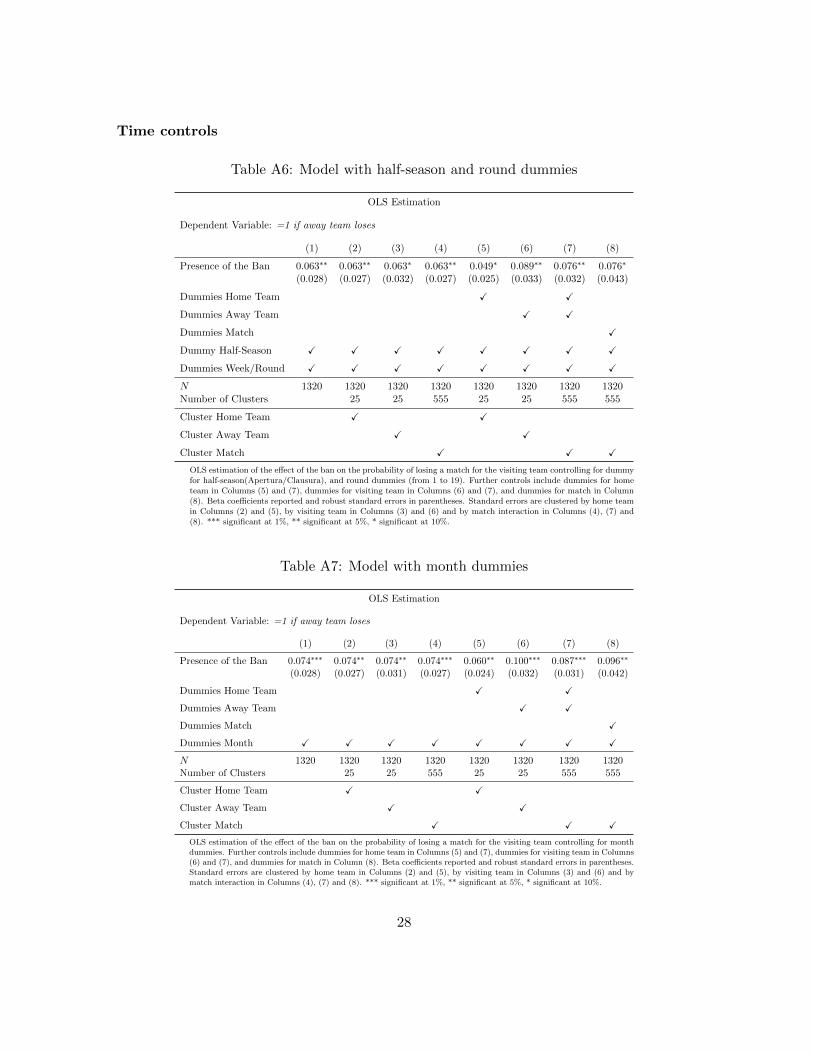
Time controls

Table A6: Model with half-season and round dummies

OLS Estimation


(1) (2) (3) (4) (5) (6) (7) (8)

Presence of the Ban 0.063∗∗ 0.063∗∗ 0.063∗ 0.063∗∗ 0.049∗ 0.089∗∗ 0.076∗∗ 0.076∗

(0.028) (0.027) (0.032) (0.027) (0.025) (0.033) (0.032) (0.043)



Dummies Match X

Dummy Half-Season X X X X X X X X

Dummies Week/Round X X X X X X X X




Cluster Match X X X

OLS estimation of the effect of the ban on the probability of losing a match for the visiting team controlling for dummyfor half-season(Apertura/Clausura), and round dummies (from 1 to 19). Further controls include dummies for hometeam in Columns (5) and (7), dummies for visiting team in Columns (6) and (7), and dummies for match in Column(8). Beta coefficients reported and robust standard errors in parentheses. Standard errors are clustered by home teamin Columns (2) and (5), by visiting team in Columns (3) and (6) and by match interaction in Columns (4), (7) and(8). *** significant at 1%, ** significant at 5%, * significant at 10%.

Table A7: Model with month dummies

OLS Estimation


(1) (2) (3) (4) (5) (6) (7) (8)

Presence of the Ban 0.074∗∗∗ 0.074∗∗ 0.074∗∗ 0.074∗∗∗ 0.060∗∗ 0.100∗∗∗ 0.087∗∗∗ 0.096∗∗

(0.028) (0.027) (0.031) (0.027) (0.024) (0.032) (0.031) (0.042)



Dummies Match X

Dummies Month X X X X X X X X




Cluster Match X X X

OLS estimation of the effect of the ban on the probability of losing a match for the visiting team controlling for monthdummies. Further controls include dummies for home team in Columns (5) and (7), dummies for visiting team in Columns(6) and (7), and dummies for match in Column (8). Beta coefficients reported and robust standard errors in parentheses.Standard errors are clustered by home team in Columns (2) and (5), by visiting team in Columns (3) and (6) and bymatch interaction in Columns (4), (7) and (8). *** significant at 1%, ** significant at 5%, * significant at 10%.

28

Tilburg University You'll Never Walk Alone Colella ... · legislation. In August 2013, as a matter...

Documents

Transcript of Tilburg University You'll Never Walk Alone Colella ... · legislation. In August 2013, as a matter...