Tier 1/IFIXX: Voltage Control Options on Low Voltage ...

Tier 1 / IFIXX (Voltage Control Options on Low Voltage Busbars)

1

Tier 1/IFIXX:

Voltage Control Options on Low Voltage Busbars

Version: 3.0

Report title:

Evaluation of voltage control options through simulations


2

Executive Summary

The aim of the voltage control options project is to deploy a range of voltage management

methods and techniques across several distribution substations which will be assessed in

terms of their ability and effectiveness to regulate line voltage in real-time in a safe and

economical manner. In addition, the ability to correct poor power factor and the feeder power

quality will also be assessed.

In order to produce the simulation model of the voltage control devices, studies need to be

carried out on operation of various voltage control options. This document describes the

operation principles and device schematics of the voltage control devices trialled for this

project. The results are also shown in the report.

In addition, due to increasing amount of distributed generation in the network, the simulation

model of active and reactive power controlled photovoltaic generator are also presented in

this report. The actual photovoltaic penetrations on the six trialled network are also discussed.

The works described in this document will provide detailed study on each voltage control

options in order to produce simulation models. The importance on distributed generation on

existing network is also being discussed.


3

Table of Contents:

1. Design and implementation of simulation models for evaluating the voltage control

algorithms .................................................................................................................................. 6

1.1 Introduction ................................................................................................................. 6

1.2 Modelling of active filter............................................................................................. 6

1.3 Modelling of distribution transformer with OLTC ................................................... 10

1.4 Modelling of powerPerfector (pP) unit ..................................................................... 18

2. Modelling of the load on the network .............................................................................. 23

2.1 A typical household load profile ............................................................................... 23

2.2 A typical household with photovoltaic...................................................................... 24

2.3 Understanding PV connected at 6 selected Electricity North West sites .................. 27

3. Conclusion ........................................................................................................................ 33


4

List of Figures:

Figure 1: Control algorithm of active filter model..................................................................... 6 Figure 2: Active filter modelling in PSCAD ............................................................................. 7 Figure 3: ABB active filter PQFS schematic ............................................................................. 8

Figure 4: ABB active filter PQFS .............................................................................................. 8 Figure 5: Control algorithm of active filter model..................................................................... 9 Figure 6: Overview of TAPCON voltage regulator ................................................................. 10 Figure 7: Voltage profile of unity tap (a) vs. -2.2% tap at Leicester Av feeder 260055783 (b)

.................................................................................................................................................. 11

Figure 8: Distribution transformer with OLTC installed for Landgate and Leicester Av

substations ................................................................................................................................ 12

Figure 9: Mayorlowe Ave Sub – WAY1 simulation model (unity load pf) ............................ 13

Figure 10: Voltage profile of different tap positions (unity load power factor) ...................... 14 Figure 11: Mayorlowe Ave Sub – WAY1 simulation model (0.97 load pf) ........................... 15 Figure 12: Voltage profile of different tap positions (0.97 load power factor) ....................... 15 Figure 13: Different load conditions comparison .................................................................... 16 Figure 14: Additional P and Q from grid to LV feeder vs. OLTC tap positions ..................... 16

Figure 15: Additional P and Q from grid to LV feeder vs. OLTC tap positions (0.97pf) ....... 17

Figure 16: powerPerfector winding configuration ................................................................... 18 Figure 17: Two winding schematic of a pP unit operation ...................................................... 19 Figure 18: Input vs. output of powerPerfector unit.................................................................. 20

Figure 19: Equivalent PSCAD model of pP+ for voltage step down and boost function ....... 21 Figure 20: powerPerfector model in PSCAD .......................................................................... 21

Figure 21: powerPerfector unit feeder connection ................................................................... 22 Figure 22: powerPerfector unit installed at Edge Green Lane substation ............................... 23

Figure 23: An example of Elexon load profile from 2010....................................................... 23 Figure 24: PV system schematic .............................................................................................. 24 Figure 25: PV system control schematic ................................................................................. 24

Figure 26: Mayorlowe Ave network with PV connection ....................................................... 25 Figure 27: Mayorlowe Ave Sub WAY1 with PV connection vs without PV ......................... 25

Figure 28: Single line study with PV connection .................................................................... 26 Figure 29: Effect of PV on single line ..................................................................................... 26 Figure 30: Voltage unbalance and harmonics .......................................................................... 27 Figure 31: Theoretical PV generation and load matching profile............................................ 28

Figure 32: Total PV and load number of all feeders ................................................................ 32

Figure 33: Total PV rating and load demand of all feeders ..................................................... 33


5

List of Tables:

Table 1: Mayorlowe Ave cable lengths ................................................................................... 13 Table 2: P and Q injection (1pf) .............................................................................................. 16 Table 3: P&Q at transformer output (0.97 load pf) ................................................................. 17

Table 4: powerPerfector unit operation ................................................................................... 20 Table 5: PV connections at Howard St .................................................................................... 27 Table 6: PV connections at Landgate ...................................................................................... 28 Table 7: PV connections at Landgate WAY7 .......................................................................... 29 Table 8: PV connections at Leicester Ave ............................................................................... 30

Table 9: PV connections at Edge Green Lane ......................................................................... 30 Table 10: PV connections at Dunton Green ............................................................................ 31


6

1. Design and implementation of simulation models for evaluating the voltage control

algorithms

1.1 Introduction

In order to implement voltage control topologies into the LV network, this report reviewed

several voltage control options. The operation topologies of varies voltage control options

such as distribution transformer with On Load Tap Changer (OLTC), powerPerfectors (pP)

and active filters are described in order to produce the equivalent simulation models. The

studies are based on the manufacturer datasheets and patent documents to give accurate

understanding.

1.2 Modelling of active filter

To simulate the behaviour of an active filter, a model was developed in PSCAD/EMTDC

based on the method proposed by [1] in 1991. The control algorithm of the model for

harmonic compensation is shown in Figure 1. Va, Vb and Vc are the voltage at the connection

bus, Ia, Ib, and Ic are the three phase ac currents at the harmonic load. The phase voltages and

currents are first measured and converted into p and q components, and then a filter is used to

filter out the instantaneous components. The harmonic current is calculated and then used by

an inverter PWM to force the compensation current into the network.

Figure 1: Control algorithm of active filter model

The load in the model is also acting as a harmonic source, where the active filter is connected

in parallel with it. The main circuit is a three phase voltage source PWM inverter using six

IGBTs. The PWM inverter has a dc capacitor. An LC filter (LR, CR) is used to suppress

switching ripples generated by the active filter. The active filter schematic in Figure 1 is

modelled in PSCAD/EMTDC software and shown in Figure 2.


7

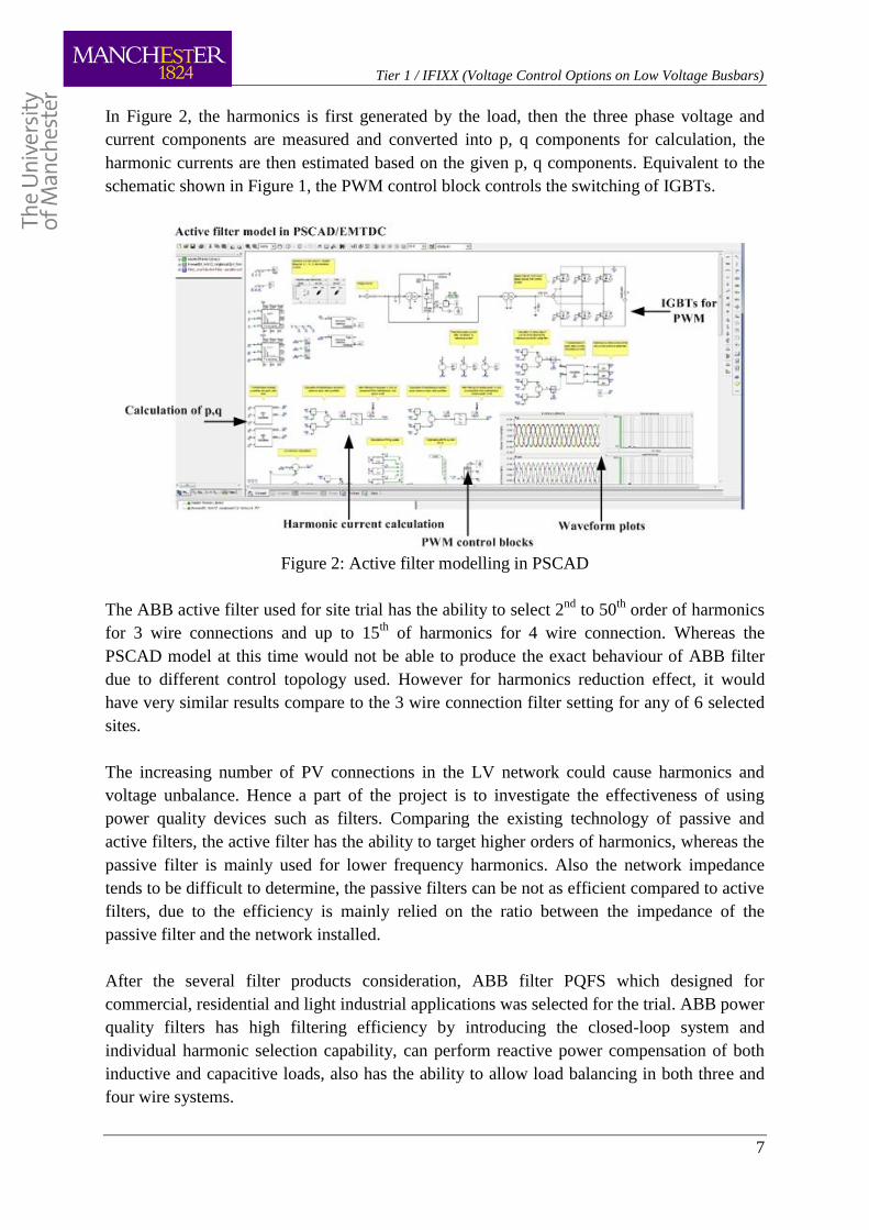
In Figure 2, the harmonics is first generated by the load, then the three phase voltage and

current components are measured and converted into p, q components for calculation, the

harmonic currents are then estimated based on the given p, q components. Equivalent to the

schematic shown in Figure 1, the PWM control block controls the switching of IGBTs.

Figure 2: Active filter modelling in PSCAD

The ABB active filter used for site trial has the ability to select 2nd

to 50th

order of harmonics

for 3 wire connections and up to 15th

of harmonics for 4 wire connection. Whereas the

PSCAD model at this time would not be able to produce the exact behaviour of ABB filter

due to different control topology used. However for harmonics reduction effect, it would

have very similar results compare to the 3 wire connection filter setting for any of 6 selected

sites.

The increasing number of PV connections in the LV network could cause harmonics and

voltage unbalance. Hence a part of the project is to investigate the effectiveness of using

power quality devices such as filters. Comparing the existing technology of passive and

active filters, the active filter has the ability to target higher orders of harmonics, whereas the

passive filter is mainly used for lower frequency harmonics. Also the network impedance

tends to be difficult to determine, the passive filters can be not as efficient compared to active

filters, due to the efficiency is mainly relied on the ratio between the impedance of the

passive filter and the network installed.

After the several filter products consideration, ABB filter PQFS which designed for

commercial, residential and light industrial applications was selected for the trial. ABB power

quality filters has high filtering efficiency by introducing the closed-loop system and

individual harmonic selection capability, can perform reactive power compensation of both

inductive and capacitive loads, also has the ability to allow load balancing in both three and

four wire systems.


8

The schematic of PQFS filter connection is shown in Figure 3. The input of the equipment is

connected with a current transformer (CT) which determines the current measurement. The

output feeds a compensation current into the network to reduce the harmonics. The filter

controller determines the anti-harmonic current to be injected based on the line current

measurements and the requirements from user. The equipment can also be set as either three

or four wire operation. Four-wire connection (three phase plus neutral) have the additional

function of voltage balancing compare to three-wire connection.

Figure 3: ABB active filter PQFS schematic

As shown in Figure 3, the line current measurements are obtained from the CT, which must

be connected upstream of the connection point of the filter and the loads. PQF current

generator converts the control signals generated by the filter controller into the filter

compensation current. The current generator is connected in parallel with the loads. The

detailed PQF main controller and current generator are shown in Figure 4 which consists of

an IGBT inverter.

Figure 4: ABB active filter PQFS


9

Information is sent to the IGBT from the filter controller. Each current generator consists of

an IGBT inverter bridge controlled by the PWM switching technology. The output of the

inverter generates a voltage waveform which contains the desired spectral components and

high frequency noise due to the IGBT switching. The PWM reactor and a high frequency

filter forms a coupling impedance. The high frequency rejection filter ensures the high

frequency noise is absorbed. The DC bus capacitor acts as storage reservoirs. The preload

resistor charges the DC capacitors once the auxiliary fuse box is closed, which prevents

excessive inrush currents at the filter start-up. In addition, up to four PQFS units may be

connected in parallel in one filter unit, one act as the master while others referred to as the

slave units.

To be able to simulate such equipment into PSCAD model, a typical active filter model based

on the method proposed by [1] was used. The control algorithm of the model for harmonic

compensation is shown in Figure 5. Va, Vb and Vc are the voltage at the connection bus, Ia, Ib,

and Ic are the three phase ac currents at the harmonic load. The phase voltages and currents

are first measured and converted into p and q components, and then a filter is used to filter

out the instantaneous components. The harmonic current is calculated and then used by an

inverter PWM to force the compensation current into the network.

Figure 5: Control algorithm of active filter model

The load in the model is also acting as a harmonic source, where the active filter is connected

in parallel with it. The main circuit is a three phase voltage source PWM inverter using six

IGBTs. The PWM inverter has a dc capacitor. An LC filter (LR, CR) is used to suppress

switching ripples generated by the active filter. When the active filter model has been

connected to the Electricity North West network model, the majority of the harmonics are

produced by the PVs from the network, hence the load shown in Figure 5 is removed.

The sites selected for this trial are at Dunton Green substation site (feeder feature number

260055770, 260055773, 260055780 and 260055783), and Howard Street substation site

(feeder feature number 216044694 and 216044696). Before each site trial, a pre-installation

data such as voltage, current and THD were collected by installing monitoring equipment.

After the active filter installation, similar set of data were again collected to carry out


10

comparison with the previous data. Each trial action will access a different filter setting such

as voltage balancing and harmonics filtering.

1.3 Modelling of distribution transformer with OLTC

There are very few distribution transformers with OLTC commercially available in the UK,

traditionally the tap position could only be changed when the transformer is off load. In

addition, the X/R ratio in LV distribution system is much lower than the HV system since LV

network mainly consists of resistive cables. Therefore, the control schemes based on reactive

power compensation and OLTCs in theory become less effective to regulate busbar voltages

in LV networks compare to MV networks. Their effectiveness will be investigated for this

voltage regulation project.

Several transformers with OLTC were considered for this voltage control options project, the

Maschinenfabrik Reinhausen (MR) iPOWER System was considered and system has the

ability to provide transformation, actuator, regulator, sensor, communication, data

management and intelligence system components for local substations.

MR voltage regulator TAPCON 230 pro was installed for the site trial, it is able to keep

constant the output voltage of a transformer with an OLTC. As shown in Figure 6, the device

compares the measured transformer output voltage with a defined desired voltage set point

[2]. The difference between the two voltages is the control deviation, if it is greater than

specified bandwidth, the device will emit a switching pulse after a defined delay time. The

switching pulse triggers a tap change which corrects the output voltage of the transformer.

The device parameters can be optimally adjusted to the line voltage behaviour to achieve a

balanced control response with a small number of tap-change operations of the OLTC [2].

Figure 6: Overview of TAPCON voltage regulator


11

In addition, TAPCON 230 pro will also be able to provide under voltage and overcurrent

blocking, overvoltage detection with high-speed return, line drop and voltage fluctuation

compensation. The equipment can operate in both auto and manual mode.

According to the actual settings of the tap changer transformer with nine tap positions, an

equivalent transformer with OLTC model was developed in PSCAD, the equipment model

are connected to Landgate and Leicester Av network. Figure 23 shows a tap setting of 0%

and -2.2% at Leicester Av feeder 260055783, as an example. The distribution transformer

with OLTC model is able to effectively step down the voltage by approximately 2.2% as

shown in Figure 7, such voltage can be validated against the actual voltage measurement on

the network at various cable locations. The transformer model parameters such as leakage

reactance are set according to the actual equipment datasheets.

(a) (b)

Figure 7: Voltage profile of unity tap (a) vs. -2.2% tap at Leicester Av feeder 260055783 (b)

It was found in simulation model that for different tap positions, the voltage profile steps

down in a nearly constant ratio according to the tap settings, this proves that the distribution

transformer with OLTC can effectively regulate the voltage in the LV network. The

effectiveness of the OLTC control option can be further studied with different load conditions,

this can be done by adjusting the load power factor or considering the load condition during a

sunny daytime when there are PV connected.

It was noted for heavier load conditions (lower load pf), voltages dropped more significantly

at every node in the network. The active and reactive power at transformer secondary for

different tap positions are also studied, it was found that the required active power (P)

increases with higher OLTC taps, whereas the reactive power shows very little changes. This

means that the grid needs to transfer more active power to the LV feeder with higher OLTC

tap positions.

To conclude, the distribution transformer with OLTC can effectively control the voltage

profile in the LV network, hence it is useful for voltage regulation and load demand


12

management on LV networks. In addition, for heavy loaded network there are much more

significant voltage drops, it is also useful to have voltage regulation devices such as LV

capacitors installed along the line, to achieve less significant voltage variation.

The distribution transformer with OLTC unit installed for this project also has the ability to

alter the tap settings automatically based on the instant voltage monitoring, as the load profile

is changing constantly. Whereas in the simulation model, the loads are considered as a

passive element for each simulation cycle, therefore it is not possible to implement the

automatic tap changing function of the OLTC. The each tap setting will be adjusted manually

for different case scenarios. Hence the project final objective is to evaluate the effectiveness

of transformer with OLTC for LV network, based on several different load conditions.

Figure 8: Distribution transformer with OLTC installed for Landgate and Leicester Av

substations

The effectiveness of using distribution transformer with OLTC on Electricity North West

network, a model for Mayorlowe Ave feeder Way1 was used to briefly investigate the effect

of different tap change position on the network as shown in Figure 9.


13

11kV

A

B C D E

12kW 27kW 1kW 9kW

2kW

2kW

8kW 2kW 2kW 2kW 6kW

2kW 2kW

5kW 7kW 1kW 2kW 1kW

F G L M N P Q

J K

R S T U V

L1

L2 L3 L4 L5

L6 L7 L8 L10 L11 L12 L13

L14

L16

L15

L17 L18 L19 L20

Mayorlowe Ave Sub – WAY1

L9H

OLTC Transformer (TX)

Figure 9: Mayorlowe Ave Sub – WAY1 simulation model (unity load pf)

The network shown in Figure 9 was simulated using PSCAD/EMTDC. In order to simplify

the network for analysis, the distributed loads along the line L1-L20 (Table 1) are being

considered as end loads at each node A-V. The output from 11kV/415V transformer (TX) is

the source, considering the network without any local distributed generation. The load is

considered to be at the maximum load demand condition (ADMD). The cable distances are

shown in Table 1.

Table 1: Mayorlowe Ave cable lengths

Line Cable description Length (m)

L1 3c 300 Consac 4

L2 0.1 Cu PILC (SNE) 189




















14

The simulation started with the transformer with OLTC tap position at 0%. The tap position

can then be changed to 1.25%, 2.5%, 3.75% and 5%, a snapshot of the voltage profile in per

unit of each node was simulated and plotted as shown in Figure 10.

Figure 10: Voltage profile of different tap positions (unity load power factor)

For different tap positions, the voltage profile steps up in a constant ratio, this proves that the

transformer with OLTC can effectively regulate the voltage in the LV network. The node SS

in Figure 10 gives the output voltage from the transformer TX secondary, it can be noted that

the voltages are just below 1.05, 1.0375, 1.025, 1.0125 and 1 per unit. Due to heavy load of

12kW and 27kW at node B and C, the voltage dropped more significantly for each tap

position. In real case, the majority of the load would be distributed along the line L2 and L3,

allowing a more smooth voltage decrease (smaller line slope between nodes A and C).

The second part of the study considers all the loads in the network have a 0.97 power factor,

the modified network schematic is shown in Figure 11. By repeating the simulation described

previously, the voltage profiles were again plotted by changing the OLTC tap position at

1.25%, 2.5%, 3.75% and 5%, this is shown in Figure 12.


15

11kV

A

B C D E

12kW

3.01kVAR

27kW

6.767kVAR

1kW

0.251kVAR9kW

2.256kVAR

2kW

0.501kVAR8kW

2.005kVAR

6kW

1.504kVAR

5kW

1.253kVAR

7kW

1.754kVAR

F G L M N P Q

J K

R S T U V

L1

L2 L3 L4 L5

L6 L7 L8 L10 L11 L12 L13

L14

L16

L15

L17 L18 L19 L20

Mayorlowe Ave Sub – WAY1

L9H

OLTC Transformer (TX)

2kW

0.501kVAR

2kW

0.501kVAR

2kW

0.501kVAR

2kW

0.501kVAR

1kW

0.251kVAR

1kW

0.251kVAR

2kW

0.501kVAR

2kW

0.501kVAR

2kW

0.501kVAR Figure 11: Mayorlowe Ave Sub – WAY1 simulation model (0.97 load pf)

Figure 12: Voltage profile of different tap positions (0.97 load power factor)

Figure 12 shows that the voltages dropped more significantly due to the heavier loads

(0.97pf), in which case is being considered as the worst scenario at the maximum load

demand. Comparing the unity power factor load and the load having a 0.97 power factor, two

models were simulated for 1pf load and 0.97pf load accordingly.


16

Figure 13: Different load conditions comparison

As shown in Figure 13, the voltages dropped more significantly at every node in the network

for loads with 0.97 power factor.

The active and reactive power at transformer secondary for different tap positions are given

in Table 2, it can be noted that the required active power (P) increases with higher OLTC taps,

the difference in active power between 0% tap position and 5% is approximately 9.32kW as

shown in Figure 14, whereas the reactive power shows very little changes (Table 2).

Table 2: P and Q injection (1pf)

P (kW) Q (kVAR)

Tap at 0% 91.18 0.4307

Tap at +1.25% 93.47 0.4415

Tap at +2.5% 95.79 0.4525

Tap at +3.75% 98.13 0.4635

Tap at +5% 100.5 0.4748

Figure 14: Additional P and Q from grid to LV feeder vs. OLTC tap positions


17

Figure 14 shows that the grid needs to transfer more active power to the LV feeder with

higher OLTC tap positions. In the case of 0.97 load power factor, the active and reactive

power at the distribution transformer secondary for different tap positions are given in Table

3. The difference in active power between 0% tap and 5% is approximately 9.13kW as shown

in Figure 15. However the difference in reactive power in this case is 2.29kVAR due to the

load reactance.

Table 3: P&Q at transformer output (0.97 load pf)

P (kW) Q (kVAR)

Tap at 0% 90.17 22.62

Tap at +1.25% 92.42 23.19

Tap at +2.5% 94.68 23.76

Tap at +3.75% 96.98 24.33

Tap at +5% 99.3 24.91

Figure 15: Additional P and Q from grid to LV feeder vs. OLTC tap positions (0.97pf)

To conclude, the distribution transformer with OLTC can effectively control the voltage

profile in the LV network, hence it is useful for voltage regulation and load demand

management on LV networks. In addition, for heavy loaded network there are much more

significant voltage drops, it is also useful to have voltage regulation devices such as LV

capacitors installed along the line, to achieve less significant voltage variation.

The standard distribution transformer with model in PSCAD will be considered for

implementation in the six selected LV networks. Due to the load used in the simulation

package is implemented as a passive component, this information is obtained by a typical

maximum and minimum load profile for each feeder, such implementation would produce the

an approximate voltage profile snapshot for each of the network based on the load demand at

a given time and a day.


18

The distribution transformer with OLTC unit installed for this project has the ability to alter

the tap settings automatically based on the instant measurement, as the load profile is

changing constantly. Whereas in the simulation model, the loads are considered to be fixed

for each simulation cycle, therefore it is not possible to implement the automatic tap changing

function of the OLTC. The each tap setting will be adjusted manually for different case

scenarios. Hence the project final recommendations will be based on the unit effectiveness

for several different load conditions, in addition to the conditions when the monitoring data is

being obtained.

1.4 Modelling of powerPerfector (pP) unit

As stated by manufacturer, the powerPerfector (pP) is designed to address a number of

common power supply problems. Optimising voltages reduces the reactance of some

electrical equipment, therefore overall improvement in power factor. The main benefit of

installing pP+ units is to maintain a stabilised output voltage for the load. In addition, the unit

is connected at the transformer secondary and has the ability to tap-changing feeder voltage

without the need to replace the existing transformer. The winding schematic of the pP was

shown in Figure 16.

Figure 16: powerPerfector winding configuration

In Figure 16, the primary winding is connected in series with the incoming power supply and

carries the load current on each phase, it is also constructed with low impedance and low

losses. This primary winding acts to filter harmonics entering the site from outside and is

rated to withstand transients up to 25kV, protecting the site from common external transient

events.

The interaction between the primary and secondary winding on each phase acts to reduce the

voltage by a fixed percentage. For example if input is 240V, output will be around 220V,

assuming an -8% optimisation setting. The connection between each phase has a current

flowing that is proportional to the difference between the three phase voltages. This

connection forms an unreferenced star point on the secondary as shown in Figure 16. By


19

configuring the pP in such way, it would be able to compensate the imbalanced phase

voltages without additional electronic or mechanical components. These are connected as a

closed delta configuration. The purpose of the closed loop is to provide a path to circulate

and dissipate harmonic currents on the input, thus attenuating and preventing them from

circulating into the downstream load (output). This winding has the same effect on harmonic

currents that are generated downstream of the pP unit, preventing harmonic currents on site

from circulating into the upstream load. The powerPerfector automatically adjusts a voltage

within a predetermined range to make stable output.

Figure 17: Two winding schematic of a pP unit operation

The schematic of the powerPerfector operation is as shown in Figure 17, where L1, L2, L5 and

L6 are the main coils, R and T are the input terminals, L3, L4, L7 and L8 are the exciting coil, r

and t are the output terminals, zero phase N and n are connected to one another. Thyristors

(1)-(8) are connected between coils respectively.

Thyristor 1 is connected between main coil L6 and exciting coil L3, thyristor 2 is connected

between main coil L2 and exciting coil L7, thyristor 3 is connected between main coil L2 and

exciting coil L3, thyristor 4 is connected between main coil L6 and exciting coil L7, thyristor 5

is connected between the exciting coil L3 and L7, thyristor 6 is connected between the

exciting coil L4 and L8, thyristor 7 is connected between main coil L2 and exciting coil L4,

and thyristor 8 is connected between main coil L6 and exciting coil L8. The thyristors are

switched ON/OFF by the voltage value detected in the voltage sensor. Figure 18 illustrates

the input and output voltage of a typical pP unit.


20

Figure 18: Input vs. output of powerPerfector unit

Assume the winding are defined as 0%, 3% and 6% drop or boost, the minimum voltage level

is set at 95V with the input voltage at 100V. As shown in Figure 18, R and T are two input

terminals, the voltage control operation is as shown in Table 4. Thyristors 1 and 2 are

switched on during voltage boost mode, and thyristors 3 and 4 are switched on for voltage

step down mode.

Table 4: powerPerfector unit operation

Input

voltage

(R&T)

Thyristor

ON

Main coil Exciting coil Voltage

Drop/Boost

(R+T)

Output voltage

(r&t)

105V 3,4,5 L1,L2,L5,L6 L3,L7 3V*4=12V (105V*2-12V)/2=99V

100V 3,4,6 L1,L2,L5,L6 L3,L4,L7,L8 1.5V*4=6V (100V*2-6V)/2=97V

98V 3,4,7,8 L1&L2,L5&L6 L3&L4,L7&L8 0V 98V

95V 1,2,6 L1,L2,L5,L6 L3,L4,L7,L8 1.5V*4=6V (95V*2+6V)/2=98V

90V 1,2,5 L1,L2,L5,L6 L3,L7 3V*4=12V (90V*2+12V)/2=96V

93V 1,2,6 L1,L2,L5,L6 L3,L4,L7,L8 1.5V*4=6V (93V*2+6V)/2=96V

96V 3,4,7,8 L1&L2,L5&L6 L3&L4,L7&L8 0V 96V

99V 3,4,6 L1,L2,L5,L6 L3,L7 3V*4=12V (99V*2+12V)/2=105V

Based on the pP winding configurations, two equivalent PSCAD models are developed by

UM, due to the pP unit uses different winding configuration for step down function in Figure

19(a) and boost function in Figure 19(b). The boost winding configuration was developed

based on the patent document from powerPerfector.


21

(a) (b)

Figure 19: Equivalent PSCAD model of pP+ for voltage step down and boost function

Figure 20: powerPerfector model in PSCAD

To be able to analyse this behaviour of pP unit, the specific details needs to be studied in

order to understand the basic principle of the equipment. Figure 21 shows the installation

configuration of the pP on site, the units are installed on the feeders at Greenside and Edge

Green Lane substation. The data can be monitored by connecting a Power Quality Meter

(PQM) at upstream and downstream of the pP unit. A link box is installed so that the pP unit

can be bypassed if needed.


22

Figure 21: powerPerfector unit feeder connection

Two 350kVA powerPerfector units are installed for site trials. The first will automatically

increase the voltage by 4%, maintain the voltage at 0% or decrease the voltage by -4%, -8%

and -12% according to the pre-set voltage reference level. The latter will automatically

increase the voltage by 2.7%, maintain the voltage at 0% or decrease the voltage by -2.7%, -

5.4% and -8.1%. The voltage tap is achieved by the thyristor based Automatic Voltage

Controller (AVC) connected in parallel to the optimiser, which will react with a time delay of

between 4 and 10 seconds before it responds to any change in the incoming voltage to avoid

hunting. Switching will occur in 0.001 seconds. The model parameters such as leakage

reactance are configured according to the datasheets received from the manufacturer.

The two network site developed for pP equipment trials are Greenside Lane and Edge Green

Lane. Similarly to other voltage regulation equipment trial, voltage, current, real and reactive

powers are recorded before and after the equipment installation. In addition to this monitoring

circuit, there are two PQM meters which are installed for each pP unit, which are connected

to input and output of the pP respectively. The pP unit can also be set in either auto or manual

operation mode, both settings are accessed during the site trial. A link box was also installed

by Electricity North West to allow redirection of the electrical supply through an alternative

route to the load, thereby allowing the unit to be taken out of circuit, hence the network can

also be operated without the pP+ unit if needed. Figure 22 shows the pP+ unit installed at

Edge Green substation.


23

Figure 22: powerPerfector unit installed at Edge Green Lane substation

2. Modelling of the load on the network

2.1 A typical household load profile

As the actual load profile at any points in the network changes constantly, the simulation

model needs to be adjusted in order to be more closed to a realistic scenario. Figure 23 shows

an example of peak load demand from Elexon for 2010. Such data would allow a snapshot of

the voltage profile at any time of the day in a year (half an hour interval). Therefore a typical

winter and summer load profile can be implemented separately in the network model. It

maximum and minimum load demand per customer was assumed to be between 0.5kW and

1kW, in some cases at 1.5W for the worst scenario.

Figure 23: An example of Elexon load profile from 2010


24

2.2 A typical household with photovoltaic

It was understood that for the selected Electricity North West sites, there are increasing

number of the household has PV installed. When the PV output exceeds the load demand, the

active power would feed back into the network at one phase. Therefore to create the load

model for Electricity North West network, a single phase PV model is needed.

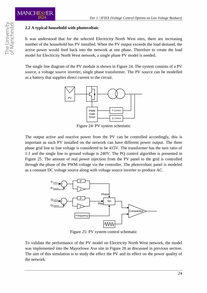
The single line diagram of the PV module is shown in Figure 24. The system consists of a PV

source, a voltage source inverter, single phase transformer. The PV source can be modelled

as a battery that supplies direct current to the circuit.

PV

P Control

Q Control

PWM

Gate

Drive

Figure 24: PV system schematic

The output active and reactive power from the PV can be controlled accordingly, this is

important as each PV installed on the network can have different power output. The three

phase grid line to line voltage is considered to be 415V. The transformer has the turn ratio of

1:1 and the single line to ground voltage is 240V. The PQ control algorithm is presented in

Figure 25. The amount of real power injection from the PV panel to the grid is controlled

through the phase of the PWM voltage via the controller. The photovoltaic panel is modeled

as a constant DC voltage source along with voltage source inverter to produce AC.

P

I

Pcontrol

+-

P

I

+-

Sin

Pmeasure

Qcontrol

Qmeasure

Comparator

Frequency

Phase

Mag

Figure 25: PV system control schematic

To validate the performance of the PV model on Electricity North West network, the model

was implemented into the Mayorlowe Ave site in Figure 26 as discussed in previous section.

The aim of this simulation is to study the effect the PV and its effect on the power quality of

the network.


25

Figure 26: Mayorlowe Ave network with PV connection

The voltage measurements are recorded at node E, Q, K and V shown in Figure 26, the nodes

are at end of each line where the voltage drop considered being at most significant. The

voltage profiles at Mayorlowe Ave with and without the PV connections are shown in Figure

27.

Figure 27: Mayorlowe Ave Sub WAY1 with PV connection vs without PV

In Figure 27, the voltage profile when the PVs are connected is higher than the one that

without, as the load demand is reduced due to the PV connection. However it is difficult to

analyse the effect on particular line in this voltage plot. To simplify the network shown in

Figure 26, only one line is considered to further analyse the effects of PV (Figure 28).


26

Figure 28: Single line study with PV connection

Figure 29: Effect of PV on single line

In can be noted from Figure 29 that the voltage profile in general has less significant drops

with increasing number of PV connected, hence having a PV installed has great benefits from

the household perspective, as less power are needed from the grid. However for network

DNOs, such effect would make the LV network voltages very difficult to determine. In

addition, due to the properties are connected per phase, each household may decide on

whichever sizes of the PV they prefer to install. Having different sizes of PV for each phase

on a three phase system would cause voltage unbalance, particular when the PVs are

operating at most their efficient (i.e daytime with sufficient sunlight).


27

Figure 30: Voltage unbalance and harmonics

In addition to the voltage unbalance, the switching components from the PV inverter could

feed back into the network as shown in Figure 30. Due to most of the selected feeders (31

feeders) has PV installed, to implement this PV into the model becomes essential to analyses

the network conditions. The details of the PV installed on the selected 31 feeders are given in

the next section.

2.3 Understanding PV connected at 6 selected Electricity North West sites

In order to understand the maximum PV output from each feeder, the number of PV

connections and their maximum output are summarised in Table 5 - Table 10. Table 5 shows

the PV connection at Howard Street. According to the data from the Electricity North West

network design sheets, there are 52 houses connected to WAY2 and 115 houses connected

for WAY3. Assume all loads are domestic restricted with ADMD of 1.5kW, the maximum

load demand for WAY2 would be 78kW and 172.5kW for WAY3. However the maximum

load demand tends to be in the evening (Figure 31), whereas the PV is most efficient during

the morning, therefore it is likely that the active power P will be injected back into the LV

network during the day time with sufficient sunlight.

Table 5: PV connections at Howard St

Howard St WAY 2

Phase A Phase B Phase C Total (kW)

1.25 kW 5 7 6 22.5 kW

2 kW 4 6 5 30 kW

52.5 kW

Howard St WAY 3


1.25 kW 7 7 6 25 kW


28

1.75 kW 1 1 - 3.5 kW

2 kW 3 0 3 12 kW

2.5 kW 1 2 1 10 kW

50.5 kW

Considering the PV connection at Landgate in Table 6, there are 49 houses connected to

WAY2, 28 and 30 houses for WAY3 and WAY4, 99 and 59 houses connected to WAY5 and

WAY6, and 75 houses connected to WAY7. Since WAY5 and WAY6 have the biggest

number of PVs connected, it is likely that the two feeders will have the most significant

voltage unbalancing and harmonic distortion.

Therefore during the daytime when there is sufficient sunlight, any power that generated by

PV which surpass the load demand at any time will be feed back into the network. The

network operator is then becomes responsible for the instantaneous load balancing and

reducing the harmonics caused by the PV inverters. This becomes challenging as DNO will

need to increase the amount of the monitoring at low voltage level, as the exact output from

PVs per phases are unknown.

Power

24 hours

Load

demand

PV output

Figure 31: Theoretical PV generation and load matching profile

Cullen et al [3] studied the risk associated with islanding of PV system within low voltage

distribution network. The report stated that in real case the load and generation profiles are

more dynamic than that shown in Figure 31. The rate of load change greater than PV output

change rate, hence there will be more load and generation matching period. However the

majority of the changes are due to transient loads, therefore it does not last very long (e.g.

<1s). In addition, the load has lagging power factor whereas the PV normally has leading

power factor. Therefore the PV output will always be noticeable in the network during the

period of low load demand. Table 6 and Table 7 list the number of PV connected at

Landgate.

Table 6: PV connections at Landgate

Landgate WAY 2

Phase A Phase B Phase C Unknown Total (kW)

2 kW 4 1 4 - 18 kW

2.5 kW - - 1 - 2.5 kW


29

2.88 kW 1 - 1 - 5.76 kW

3 kW - 3 - - 9 kW

3.2 kW 1 3 - - 12.8 kW

48.06 kW

Landgate WAY 3


2 kW 1 1 1 1 8 kW

2.5 kW 1 1 - 1 7.5 kW

2.66 kW - - 1 - 2.66 kW

3 kW 1 - - - 3 kW

3.2 kW - 1 - - 3.2 kW

24.36 kW

Landgate WAY 4


2 kW - - - 2 4 kW

2.28 kW - 1 - - 2.28 kW

2.5 kW - - - 1 2.5 kW

3 kW - - - 2 6 kW

14.78 kW

Landgate WAY 5


2 kW 2 4 4 1 22 kW

2.5 kW 3 2 2 - 17.5 kW

3 kW 1 1 2 - 12 kW

3.2 kW - 1 1 - 6.4 kW

57.9 kW

Landgate WAY 6


2 kW 1 - 1 - 4 kW

2.5 kW 2 - - - 5 kW

3 kW 4 - 4 2 36 kW

3.2 kW 3 2 - - 16 kW

61 kW

Table 7: PV connections at Landgate WAY7

Landgate WAY 7


2 kW 1 - - 2 6 kW

2.28 kW 1 - - - 2.28 kW

2.5 kW 1 1 1 - 7.5 kW

2.88 kW - 1 - - 2.88 kW

3 kW - 1 1 3 15 kW

33.66 kW


30

From Table 8, WAY2 of Leicester Ave has the most number of PV connected. The number

of domestic type of load on WAY2 is around 31. Hence there is likely to have a reverse

power flow on WAY2 on a sunny daytime.

Table 8: PV connections at Leicester Ave

Leicester Ave WAY 1


2.5 kW - 1 - - 2.5 kW

2.88 kW 1 - 1 7 25.92 kW

28.42 kW

Leicester Ave WAY 2


1.9 kW 2 - 1 - 5.7 kW

2.16 kW - - - 2 4.32 kW

2.28 kW - - - 1 2.28 kW

2.4 kW - 3 3 - 14.4 kW

2.64 kW 1 1 - - 5.28 kW

2.88 kW - - 1 4 14.4 kW

3.36 kW - - - 2 6.72 kW

3.4 kW 1 - - - 3.4 kW

3.56 kW 1 2 - - 10.68 kW

3.84 kW - - - 4 15.36 kW

82.54 kW

Leicester Ave WAY 3


3.36 kW - 1 - - 3.36 kW

Table 9: PV connections at Edge Green Lane

Edge Green Lane WAY 1


3.3 kW - - - 1 3.3 kW

3.36 kW - - - 1 3.36 kW

6.66 kW



2.4 kW 6 7 2 - 36 kW

2.5 kW 2 1 1 5 22.5 kW

3.3 kW 1 1 2 1 16.5 kW

75 kW



2.3 kW - - - 1 2.3 kW

2.4 kW - - - 1 2.4 kW

3.3 kW - - - 4 13.2 kW

17.9 kW


31

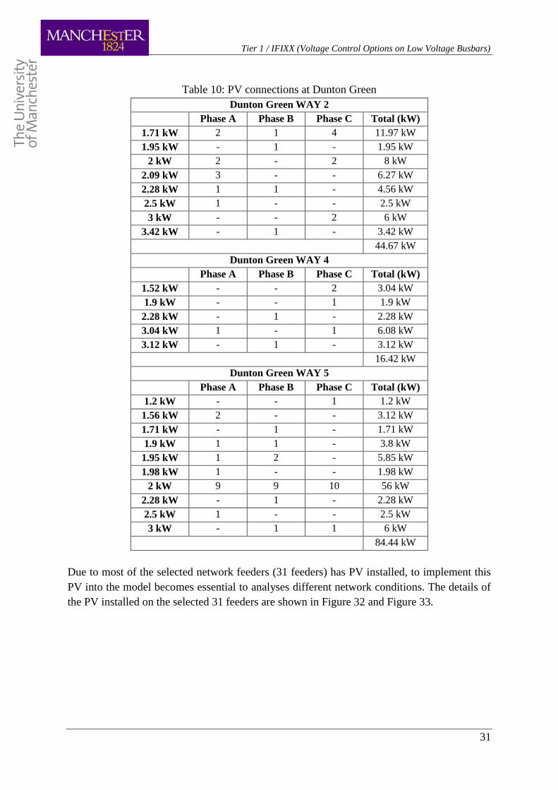
Table 10: PV connections at Dunton Green

Dunton Green WAY 2


1.71 kW 2 1 4 11.97 kW

1.95 kW - 1 - 1.95 kW

2 kW 2 - 2 8 kW

2.09 kW 3 - - 6.27 kW

2.28 kW 1 1 - 4.56 kW

2.5 kW 1 - - 2.5 kW

3 kW - - 2 6 kW

3.42 kW - 1 - 3.42 kW

44.67 kW

Dunton Green WAY 4


1.52 kW - - 2 3.04 kW

1.9 kW - - 1 1.9 kW

2.28 kW - 1 - 2.28 kW

3.04 kW 1 - 1 6.08 kW

3.12 kW - 1 - 3.12 kW

16.42 kW

Dunton Green WAY 5


1.2 kW - - 1 1.2 kW

1.56 kW 2 - - 3.12 kW

1.71 kW - 1 - 1.71 kW

1.9 kW 1 1 - 3.8 kW

1.95 kW 1 2 - 5.85 kW

1.98 kW 1 - - 1.98 kW

2 kW 9 9 10 56 kW

2.28 kW - 1 - 2.28 kW

2.5 kW 1 - - 2.5 kW

3 kW - 1 1 6 kW

84.44 kW

Due to most of the selected network feeders (31 feeders) has PV installed, to implement this

PV into the model becomes essential to analyses different network conditions. The details of

the PV installed on the selected 31 feeders are shown in Figure 32 and Figure 33.


32

Figure 32: Total PV and load number of all feeders

In order to understand the maximum PV output from each feeder, the number of PV

connections and their maximum ratings are summarised in Figure 32 and Figure 33

respectively. Figure 32 shows the number of houses connected to each feeder against the

number of PVs connected. It can be noted that a significant proportion of the trialled feeders

has the PV installed.

Assuming a 0.5kW ADMD for each house, the maximum load against the maximum PV

rating is shown in Figure 33. This can be treated as the scenario around the noon when the

load demand is relatively low and the PVs are at their most efficient. Hence in this particular

case, the network is likely to be able to sustain itself with some of the power (P&Q) likely to

reverse back into the grid. This behaviour is also confirmed in the results obtained from site

trial.

The feeder 63057171 for instance in Figure 33, the estimated load demand and the maximum

PV rating is very similar (15kW and 14.78kW), the power seen at the substation end is likely

to be close to zero. In case of the feeder 260055783, the maximum PV rating greatly exceeds

the estimated load demand, therefore the substation monitoring point is likely to notice a

reverse power flow when the PVs are at their most efficient.


33

Figure 33: Total PV rating and load demand of all feeders

3. Conclusion

This report provides the information of the voltage regulation equipment modelling based on

the researches carried out so far. After the exact network models of 31 feeders been

developed, the behaviours of these models will be further validated for any given load

conditions. For active filter models in particular, its ability to reduce the harmonics generated

by PVs will be investigated against the site trial data.

It was found in the simulation that when a significant proportion of the PV being installed,

the voltage profile in general has less significant drop. Hence having a PV installed has great

benefits from the household perspective, as less power is needed from the grid to provide

energy saving. However for network DNO, such effect would make the LV network voltages

very difficult to predict.

The challenges to have large penetration of PV generation in the distribution network, is that

it could cause the voltage to exceed the statutory limits at customer, and possibly overloading

the infrastructure (distribution transformer and cables), and also cause voltage unbalance and

harmonics, some study also suggests it could also lead to failure of the protection system.

Some of the substation networks could allow higher PV capacity, while some networks have

limited capacity for PV penetration. Installing voltage control equipment would be able to

help distribution network to cope with overvoltage phenomena with higher PV penetration.


34

Reference

[1] Hideaki Fujita and Hirohmi Akagi, “A Practical Approach to Harmonic Compensation in

Power Systems - Series Connection of Passive and Active Filters” IEEE TRANSACTIONS

ON INDUSTRY APPLICATIONS, VOL. 21, NO. 6, 1991

[2] MR TAPCON 230 Manual: http://www.reinhausen.com

[3] N. Cullen, et al., "Risk analysis of islanding of photovoltaic power systems within low

voltage distribution networks," Report IEA-PVPS T5-08, 2002

[4] D. Unger, and J. Myrzik, “Analysis of various voltage control methods for low voltage

networks with distributed generators,” CIRED 21st International Conference on Electricity

Distribution, Frankfurt, Jun 2011.

[5] V. Levi, M. Kay, M. Attree, and I. Povey, "Design of low voltage networks for premises

with small scale embedded generators," CIRED 18th International Conference on Electricity

Distribution, Turin, Jun 2005.

[6] P. Kadurek, J.F.G. Cobben, and W.L. Kling, "Smart MV/LV transformer for future

grids," International Symposium on Power Electronics Electrical Drives Automation and

Motion (SPEEDAM), Pisa, Jun 2010.

[7] B.O. Brewin, S.C.E. Jupe, M.G. Bartlett, K.T. Jackson, and C. Hanmer, "New

technologies for low voltage distribution networks," IEEE PES International Conference and

Exhibition on Innovative Smart Grid Technologies (ISGT Europe), Manchester, Dec 2011.

[8] J. Morren, S.W.H. Haan, and J.A. Ferreira, "Contribution of DG units to voltage control:

Active and reactive power limitations," IEEE Russia Power Tech, St.Petersburg, Jun 2005.

[9] P. Kadurek, J.F.G. Cobben, and W.L. Kling, "Future LV distribution network design and

current practices in the Netherlands," IEEE PES International Conference and Exhibition on

Innovative Smart Grid Technologies (ISGT Europe), Manchester, Dec 2011.

[10] E. Demirok, D. Sera, R. Teodorescu, P. Rodriguez, and U. Borup, "Clustered PV

inverters in LV networks: An overview of impacts and comparison of voltage control

strategies," IEEE Electrical Power & Energy Conference (EPEC), Montreal, Oct 2009.

http://www.reinhausen.com/

Tier 1/IFIXX: Voltage Control Options on Low Voltage ...

Documents

Transcript of Tier 1/IFIXX: Voltage Control Options on Low Voltage ...