
tic structural induction seman-pcousot/publications.www/... · tic structural inductionbased on...
14
POPL 2012, An Abstract Interpretation Framework for Termination © P. Cousot & R. Cousot POPL 2012, An Abstract Interpretation Framework for Termination © P. Cousot & R. Cousot POPL 2012: 39th ACM SIGPLAN-SIGACT Symposium on Principles of Programming Languages Philadelphia, USA, January 25-27, 2012 Patrick Cousot Radhia Cousot cims.nyu.edu/~pcousot/ www.di.ens.fr/~cousot/ www.di.ens.fr/~rcousot/ An Abstract Interpretation Framework for Termination 1 POPL 2012, An Abstract Interpretation Framework for Termination © P. Cousot & R. Cousot POPL 2012, An Abstract Interpretation Framework for Termination © P. Cousot & R. Cousot Three principles 2 POPL 2012, An Abstract Interpretation Framework for Termination © P. Cousot & R. Cousot Program verification methods (formal proof or static analysis methods) are abstract interpretations of a semantics of the programming language POPL 2012, An Abstract Interpretation Framework for Termination © P. Cousot & R. Cousot Principle I P. Cousot and R. Cousot. Abstract interpretation: a unified lattice model for static analysis of programs by construction or approximation of fixpoints. POPL, 238– 252, 1977. P. Cousot and R. Cousot. Systematic design of program analysis frameworks. POPL, 269–282, 1979. P. Cousot and R. Cousot. Constructive versions of Tarski’s fixed point theorems. 3 (*) (**) (*,**) POPL 2012, An Abstract Interpretation Framework for Termination © P. Cousot & R. Cousot POPL 2012, An Abstract Interpretation Framework for Termination © P. Cousot & R. Cousot Refinement to principle II Safety as well as termination verification methods are abstract interpretations of a maximal trace semantics of the programming language 4
Transcript of tic structural induction seman-pcousot/publications.www/... · tic structural inductionbased on...

POPL 2012, An Abstract Interpretation Framework for Termination © P. Cousot & R. CousotPOPL 2012, An Abstract Interpretation Framework for Termination © P. Cousot & R. Cousot
POPL 2012: 39th ACM SIGPLAN-SIGACT Symposium on Principles of Programming Languages
Philadelphia, USA, January 25-27, 2012
Patrick Cousot Radhia Cousotcims.nyu.edu/~pcousot/www.di.ens.fr/~cousot/
www.di.ens.fr/~rcousot/
An Abstract Interpretation Framework for Termination
1
POPL 2012, An Abstract Interpretation Framework for Termination © P. Cousot & R. CousotPOPL 2012, An Abstract Interpretation Framework for Termination © P. Cousot & R. Cousot
Three principles
2
POPL 2012, An Abstract Interpretation Framework for Termination © P. Cousot & R. Cousot
Program verification methods (formal proof or static analysis methods) are abstract interpretations of a semantics of the programming language
POPL 2012, An Abstract Interpretation Framework for Termination © P. Cousot & R. Cousot
Principle I
with widening/narrowing, as considered in this paper, are definitelystrictly more powerful than finite abstractions. The computationof variant functions by abstraction is new, and di↵erent from thecounter-example guided ways to find disjunctive ranking functions,used in tools like Terminator [7] and derivatives.
18. ConclusionAbstract interpretation has established constructive principles forreasoning about semantics. A semantics is a fixpoint so proving asemantic property at some level of abstraction consists in verifyingproperties of abstract fixpoints which have to be checked (inchecking/verification methods), guessed (in proof methods), orautomatically inferred or approximated (in static analysis methods).
This principle was mainly applied in the past to invariance andindirectly to termination by reduction to invariance. We have shownthat the abstract interpretation principle directly applies to bothsafety (generalizing invariance) and termination.
Moreover we have generalized the classical syntactic structuralinduction into the language-independent semantic concept of seman-tic structural induction based on (abstractions of) inductive tracecovers which includes induction on syntax, control states, mem-ory states, and execution trace segments and thus generalizes allverification and static analysis methods.
This methodology allowed us to establish new principles forproving termination by abstract interpretation of a terminationsemantics. It remains to design a suitable collection of abstractdomains beyond the examples proposed in this paper and thecorresponding implementations.
The present abstract interpretation termination framework has tobe extended to liveness [6, 53] and more generally to inevitabilityunder fairness hypotheses [35, 52, 55].
References[1] I. Balaban, A. Pnueli, and L. Zuck. Modular ranking abstraction. Int. J. Found.
Comput. Sci., 18(1):5–44, 2007.[2] A. Biere, A. Cimatti, E. Clarke, O. Strichman, and Y. Zhu. Bounded model
checking. Advances in Computers, 58:118–149, 2003.[3] R. Burstall. Program proving as hand simulation with a little induction. Informa-
tion Processing, 308–312. North-Holland, 1974.[4] E. Clarke, O. Grumberg, and D. Peled. Model Checking. MIT Press, 1999.[5] M. Clarkson and F. Schneider. Hyperproperties. Journal of Computer Security,
18(6):1157–1210, 2010.[6] B. Cook and E. Koskinen. Making prophecies with decision predicates. POPL,
399–410, 2011.[7] B. Cook, A. Gotsman, A. Podelski, A. Rybalchenko, and M. Vardi. Proving that
programs eventually do something good. POPL, 265–276, 2007.[8] B. Cook, S. Gulwani, T. Lev-Ami, A. Rybalchenko, and M. Sagiv. Proving
conditional termination. CAV, LNCS 5123, 328–340, 2008.[9] B. Cook, A. Podelski, and A. Rybalchenko. Summarization for termination: no
return! Form. Methods Syst. Des., 35:369–387, 2009.[10] S. Cook. Soundness and completeness of an axiom system for program verifica-
tion. SIAM J. Comput., 7:70–80, 1978.[11] P. Cousot. Méthodes itératives de construction et d’approximation de points fi-
xes d’opérateurs monotones sur un treillis, analyse sémantique de programmes.Thèse d’État ès sciences math., USMG, Grenoble, 1978.
[12] P. Cousot. Semantic foundations of program analysis. Program Flow Analysis:Theory and Applications, ch. 10, 303–342. Prentice-Hall, 1981.
[13] P. Cousot. The calculational design of a generic abstract interpreter. M. Broyand R. Steinbrüggen, eds., Calculational System Design. NATO ASI Series F.IOS Press, Amsterdam, 1999.
[14] P. Cousot. Partial completeness of abstract fixpoint checking. SARA, LNCS1864, 1–25, 2000.
[15] P. Cousot. Constructive design of a hierarchy of semantics of a transition systemby abstract interpretation. TCS, 277(1–2):47–103, 2002.
[16] P. Cousot. Verification by abstract interpretation. Proc. Int. Symp. on Verification– Theory & Practice, LNCS 2772, 243–268, 2003.
[17] P. Cousot. Proving program invariance and termination by parametric abstrac-tion, Lagrangian relaxation and semidefinite programming. VMCAI, LNCS 3385,1–24, 2005.
[18] P. Cousot and R. Cousot. Static determination of dynamic properties of programs.Proc. 2nd Int. Symp. on Programming, 106–130. Dunod, Paris, 1976.
[19] P. Cousot and R. Cousot. Abstract interpretation: a unified lattice model for staticanalysis of programs by construction or approximation of fixpoints. POPL, 238–252, 1977.
[20] P. Cousot and R. Cousot. Static determination of dynamic properties of recursiveprocedures. Formal Description of Programming Concepts, 237–277. North-Holland, 1977.
[21] P. Cousot and R. Cousot. Systematic design of program analysis frameworks.POPL, 269–282, 1979.
[22] P. Cousot and R. Cousot. Constructive versions of Tarski’s fixed point theorems.P. J. of Math., 82(1):43–57, 1979.
[23] P. Cousot and R. Cousot. Induction principles for proving invariance propertiesof programs. Tools & Notions for Program Construction: an Advanced Course,75–119. Cambridge University Press, Cambridge, UK, 1982.
[24] P. Cousot and R. Cousot. “À la Floyd” induction principles for proving in-evitability properties of programs. Algebraic methods in semantics, 277–312.Cambridge University Press, Cambridge, UK, 1985.
[25] P. Cousot and R. Cousot. Sometime = always + recursion ⌘ always, on theequivalence of the intermittent and invariant assertions methods for provinginevitability properties of programs. Acta Informatica, 24:1–31, 1987.
[26] P. Cousot and R. Cousot. Abstract interpretation frameworks. JLC, 2(4):511–547, 1992.
[27] P. Cousot and R. Cousot. Comparing the Galois connection and widening/nar-rowing approaches to abstract interpretation. PLILP, LNCS 631, 269–295, 1992.
[28] P. Cousot and R. Cousot. Inductive definitions, semantics and abstract interpre-tation. POPL, 83–94, 1992.
[29] P. Cousot and R. Cousot. “À la Burstall” intermittent assertions inductionprinciples for proving inevitable ability properties of programs. TCS, 120(1):123–155, 1993.
[30] P. Cousot and R. Cousot. Higher-order abstract interpretation (and application tocomportment analysis generalizing strictness, termination, projection and PERanalysis of functional languages). Int. Conf. on Comp. Lang., 95–112, 1994.
[31] P. Cousot and N. Halbwachs. Automatic discovery of linear restraints amongvariables of a program. POPL, 84–97, 1978.
[32] P. Cousot, R. Cousot, and L. Mauborgne. A scalable segmented decision treeabstract domain. Time for Verification, Essays in Memory of A. Pnueli, LNCS6200, 72–95, 2010.
[33] P. Cousot, R. Cousot, and F. Logozzo. A parametric segmentation functor forfully automatic and scalable array content analysis. POPL, 105–118, 2011.
[34] P. Cousot, R. Cousot, and F. Logozzo. Precondition inference from intermittentassertions and application to contracts on collections. VMCAI, LNCS 6538, 150–168, 2011.
[35] R. Cousot. Fondements des méthodes de preuve d’invariance et de fatalité deprogrammes parallèles. Thèse d’État ès sciences math, INPL, Nancy, 1985.
[36] B. Davey and H. Priestley. Introduction to Lattices and Order, 2nd Edition.Cambridge University Press, 2002.
[37] E. Dijkstra. Guarded commands, nondeterminacy and formal derivation ofprograms. CACM, 18(8):453–457, 1975.
[38] E. Dijkstra. A Discipline of Programming. Prentice-Hall, 1976.[39] J. Feret. The arithmetic-geometric progression abstract domain. VMCAI, LNCS
3385, 42–58, 2005.[40] R. Floyd. Assigning meaning to programs. Proc. Symp. in Applied Math., Vol. 19,
19–32. Amer. Math. Soc., 1967.[41] S. Graf and H. Saïdi. Construction of abstract state graphs with PVS. CAV,
LNCS 1254, 72–83, 1997.[42] M. Heizmann, J. Hoenicke, and A. Podelski. Refinement of trace abstraction.
SAS, LNCS 5673, 69–85, 2009.[43] C. Hoare. An axiomatic basis for computer programming. Communications of
the Association for Computing Machinery, 12(10):576–580, 1969.[44] Z. Manna and A. Pnueli. Axiomatic approach to total correctness of programs.
Acta Inf., 3:243–263, 1974.[45] K. McMillan and L. Zuck. Invisible invariants and abstract interpretation. SAS,
LNCS 6887, 249–262, 2011.[46] A. Miné. The octagon abstract domain. HOSC, 19:31–100, 2006.[47] D. Monniaux. Automatic modular abstractions for template numerical con-
straints. Logical Methods in Comp. Sci., 6(3), 2010.[48] J. Morris and B. Wegbreit. Subgoal induction. CACM, 20(4):209–222, 1977.[49] P. Naur. Proofs of algorithms by general snapshots. BIT, 6:310–316, 1966.[50] D. Pataria. A constructive proof of Tarski’s fixed-point theorem for DCPO’s.
Reported by M.H. Escardó in “Joins in the frame of nuclei”, Applied CategoricalStructures 11 (2) 117–124, 2003.
[51] G. Plotkin. A structural approach to operational semantics. Technical ReportDAIMI FN-19, Aarhus University, 1981.
[52] A. Pnueli, A. Podelski, and A. Rybalchenko. Separating fairness and well-foundedness for the analysis of fair discrete systems. TACAS, LNCS 3440, 124–139, 2005.
[53] A. Podelski and A. Rybalchenko. Transition invariants. LICS, 32–41, 2004.[54] A. Podelski and A. Rybalchenko. A complete method for the synthesis of linear
ranking functions. VMCAI, LNCS 2937, 239–251, 2004.[55] A. Podelski and A. Rybalchenko. Transition predicate abstraction and fair
termination. POPL, 132–144, 2005.[56] X. Rival and L. Mauborgne. The trace partitioning abstract domain. TOPLAS,
29(5), 2007.[57] D. Scott and C. Strachey. Towards a mathematical semantics for computer
languages. Tech. rep. PRG-6, Oxford Univ. Comp. Lab., 1971.[58] A. Tarski. A lattice theoretical fixpoint theorem and its applications. P. J. of
Math., 5:285–310, 1955.[59] R. Turing. Checking a large routine. Con. on High Speed Automatic Calculating
Machines, Math. Lab., Cambridge, UK, 67–69, 1949.with widening/narrowing, as considered in this paper, are definitelystrictly more powerful than finite abstractions. The computationof variant functions by abstraction is new, and di↵erent from thecounter-example guided ways to find disjunctive ranking functions,used in tools like Terminator [7] and derivatives.
18. ConclusionAbstract interpretation has established constructive principles forreasoning about semantics. A semantics is a fixpoint so proving asemantic property at some level of abstraction consists in verifyingproperties of abstract fixpoints which have to be checked (inchecking/verification methods), guessed (in proof methods), orautomatically inferred or approximated (in static analysis methods).
This principle was mainly applied in the past to invariance andindirectly to termination by reduction to invariance. We have shownthat the abstract interpretation principle directly applies to bothsafety (generalizing invariance) and termination.
Moreover we have generalized the classical syntactic structuralinduction into the language-independent semantic concept of seman-tic structural induction based on (abstractions of) inductive tracecovers which includes induction on syntax, control states, mem-ory states, and execution trace segments and thus generalizes allverification and static analysis methods.
This methodology allowed us to establish new principles forproving termination by abstract interpretation of a terminationsemantics. It remains to design a suitable collection of abstractdomains beyond the examples proposed in this paper and thecorresponding implementations.
The present abstract interpretation termination framework has tobe extended to liveness [6, 53] and more generally to inevitabilityunder fairness hypotheses [35, 52, 55].
References[1] I. Balaban, A. Pnueli, and L. Zuck. Modular ranking abstraction. Int. J. Found.
Comput. Sci., 18(1):5–44, 2007.[2] A. Biere, A. Cimatti, E. Clarke, O. Strichman, and Y. Zhu. Bounded model
checking. Advances in Computers, 58:118–149, 2003.[3] R. Burstall. Program proving as hand simulation with a little induction. Informa-
tion Processing, 308–312. North-Holland, 1974.[4] E. Clarke, O. Grumberg, and D. Peled. Model Checking. MIT Press, 1999.[5] M. Clarkson and F. Schneider. Hyperproperties. Journal of Computer Security,
18(6):1157–1210, 2010.[6] B. Cook and E. Koskinen. Making prophecies with decision predicates. POPL,
399–410, 2011.[7] B. Cook, A. Gotsman, A. Podelski, A. Rybalchenko, and M. Vardi. Proving that
programs eventually do something good. POPL, 265–276, 2007.[8] B. Cook, S. Gulwani, T. Lev-Ami, A. Rybalchenko, and M. Sagiv. Proving
conditional termination. CAV, LNCS 5123, 328–340, 2008.[9] B. Cook, A. Podelski, and A. Rybalchenko. Summarization for termination: no
return! Form. Methods Syst. Des., 35:369–387, 2009.[10] S. Cook. Soundness and completeness of an axiom system for program verifica-
tion. SIAM J. Comput., 7:70–80, 1978.[11] P. Cousot. Méthodes itératives de construction et d’approximation de points fi-
xes d’opérateurs monotones sur un treillis, analyse sémantique de programmes.Thèse d’État ès sciences math., USMG, Grenoble, 1978.
[12] P. Cousot. Semantic foundations of program analysis. Program Flow Analysis:Theory and Applications, ch. 10, 303–342. Prentice-Hall, 1981.
[13] P. Cousot. The calculational design of a generic abstract interpreter. M. Broyand R. Steinbrüggen, eds., Calculational System Design. NATO ASI Series F.IOS Press, Amsterdam, 1999.
[14] P. Cousot. Partial completeness of abstract fixpoint checking. SARA, LNCS1864, 1–25, 2000.
[15] P. Cousot. Constructive design of a hierarchy of semantics of a transition systemby abstract interpretation. TCS, 277(1–2):47–103, 2002.
[16] P. Cousot. Verification by abstract interpretation. Proc. Int. Symp. on Verification– Theory & Practice, LNCS 2772, 243–268, 2003.
[17] P. Cousot. Proving program invariance and termination by parametric abstrac-tion, Lagrangian relaxation and semidefinite programming. VMCAI, LNCS 3385,1–24, 2005.
[18] P. Cousot and R. Cousot. Static determination of dynamic properties of programs.Proc. 2nd Int. Symp. on Programming, 106–130. Dunod, Paris, 1976.
[19] P. Cousot and R. Cousot. Abstract interpretation: a unified lattice model for staticanalysis of programs by construction or approximation of fixpoints. POPL, 238–252, 1977.
[20] P. Cousot and R. Cousot. Static determination of dynamic properties of recursiveprocedures. Formal Description of Programming Concepts, 237–277. North-Holland, 1977.
[21] P. Cousot and R. Cousot. Systematic design of program analysis frameworks.POPL, 269–282, 1979.
[22] P. Cousot and R. Cousot. Constructive versions of Tarski’s fixed point theorems.P. J. of Math., 82(1):43–57, 1979.
[23] P. Cousot and R. Cousot. Induction principles for proving invariance propertiesof programs. Tools & Notions for Program Construction: an Advanced Course,75–119. Cambridge University Press, Cambridge, UK, 1982.
[24] P. Cousot and R. Cousot. “À la Floyd” induction principles for proving in-evitability properties of programs. Algebraic methods in semantics, 277–312.Cambridge University Press, Cambridge, UK, 1985.
[25] P. Cousot and R. Cousot. Sometime = always + recursion ⌘ always, on theequivalence of the intermittent and invariant assertions methods for provinginevitability properties of programs. Acta Informatica, 24:1–31, 1987.
[26] P. Cousot and R. Cousot. Abstract interpretation frameworks. JLC, 2(4):511–547, 1992.
[27] P. Cousot and R. Cousot. Comparing the Galois connection and widening/nar-rowing approaches to abstract interpretation. PLILP, LNCS 631, 269–295, 1992.
[28] P. Cousot and R. Cousot. Inductive definitions, semantics and abstract interpre-tation. POPL, 83–94, 1992.
[29] P. Cousot and R. Cousot. “À la Burstall” intermittent assertions inductionprinciples for proving inevitable ability properties of programs. TCS, 120(1):123–155, 1993.
[30] P. Cousot and R. Cousot. Higher-order abstract interpretation (and application tocomportment analysis generalizing strictness, termination, projection and PERanalysis of functional languages). Int. Conf. on Comp. Lang., 95–112, 1994.
[31] P. Cousot and N. Halbwachs. Automatic discovery of linear restraints amongvariables of a program. POPL, 84–97, 1978.
[32] P. Cousot, R. Cousot, and L. Mauborgne. A scalable segmented decision treeabstract domain. Time for Verification, Essays in Memory of A. Pnueli, LNCS6200, 72–95, 2010.
[33] P. Cousot, R. Cousot, and F. Logozzo. A parametric segmentation functor forfully automatic and scalable array content analysis. POPL, 105–118, 2011.
[34] P. Cousot, R. Cousot, and F. Logozzo. Precondition inference from intermittentassertions and application to contracts on collections. VMCAI, LNCS 6538, 150–168, 2011.
[35] R. Cousot. Fondements des méthodes de preuve d’invariance et de fatalité deprogrammes parallèles. Thèse d’État ès sciences math, INPL, Nancy, 1985.
[36] B. Davey and H. Priestley. Introduction to Lattices and Order, 2nd Edition.Cambridge University Press, 2002.
[37] E. Dijkstra. Guarded commands, nondeterminacy and formal derivation ofprograms. CACM, 18(8):453–457, 1975.
[38] E. Dijkstra. A Discipline of Programming. Prentice-Hall, 1976.[39] J. Feret. The arithmetic-geometric progression abstract domain. VMCAI, LNCS
3385, 42–58, 2005.[40] R. Floyd. Assigning meaning to programs. Proc. Symp. in Applied Math., Vol. 19,
19–32. Amer. Math. Soc., 1967.[41] S. Graf and H. Saïdi. Construction of abstract state graphs with PVS. CAV,
LNCS 1254, 72–83, 1997.[42] M. Heizmann, J. Hoenicke, and A. Podelski. Refinement of trace abstraction.
SAS, LNCS 5673, 69–85, 2009.[43] C. Hoare. An axiomatic basis for computer programming. Communications of
the Association for Computing Machinery, 12(10):576–580, 1969.[44] Z. Manna and A. Pnueli. Axiomatic approach to total correctness of programs.
Acta Inf., 3:243–263, 1974.[45] K. McMillan and L. Zuck. Invisible invariants and abstract interpretation. SAS,
LNCS 6887, 249–262, 2011.[46] A. Miné. The octagon abstract domain. HOSC, 19:31–100, 2006.[47] D. Monniaux. Automatic modular abstractions for template numerical con-
straints. Logical Methods in Comp. Sci., 6(3), 2010.[48] J. Morris and B. Wegbreit. Subgoal induction. CACM, 20(4):209–222, 1977.[49] P. Naur. Proofs of algorithms by general snapshots. BIT, 6:310–316, 1966.[50] D. Pataria. A constructive proof of Tarski’s fixed-point theorem for DCPO’s.
Reported by M.H. Escardó in “Joins in the frame of nuclei”, Applied CategoricalStructures 11 (2) 117–124, 2003.
[51] G. Plotkin. A structural approach to operational semantics. Technical ReportDAIMI FN-19, Aarhus University, 1981.
[52] A. Pnueli, A. Podelski, and A. Rybalchenko. Separating fairness and well-foundedness for the analysis of fair discrete systems. TACAS, LNCS 3440, 124–139, 2005.
[53] A. Podelski and A. Rybalchenko. Transition invariants. LICS, 32–41, 2004.[54] A. Podelski and A. Rybalchenko. A complete method for the synthesis of linear
ranking functions. VMCAI, LNCS 2937, 239–251, 2004.[55] A. Podelski and A. Rybalchenko. Transition predicate abstraction and fair
termination. POPL, 132–144, 2005.[56] X. Rival and L. Mauborgne. The trace partitioning abstract domain. TOPLAS,
29(5), 2007.[57] D. Scott and C. Strachey. Towards a mathematical semantics for computer
languages. Tech. rep. PRG-6, Oxford Univ. Comp. Lab., 1971.[58] A. Tarski. A lattice theoretical fixpoint theorem and its applications. P. J. of
Math., 5:285–310, 1955.[59] R. Turing. Checking a large routine. Con. on High Speed Automatic Calculating
Machines, Math. Lab., Cambridge, UK, 67–69, 1949.
3
(*)
(**)
(*,**)
POPL 2012, An Abstract Interpretation Framework for Termination © P. Cousot & R. CousotPOPL 2012, An Abstract Interpretation Framework for Termination © P. Cousot & R. Cousot
Refinement to principle II
Safety as well as termination verification methods are abstract interpretations of a maximal trace semantics of the programming language
4

POPL 2012, An Abstract Interpretation Framework for Termination © P. Cousot & R. CousotPOPL 2012, An Abstract Interpretation Framework for Termination © P. Cousot & R. Cousot
Comments on principle II• This is well-known for instances of safety (like
invariance) using prefix trace semantics
• This is proved in the paper for full safety (omitted in this presentation)
• New for termination
with widening/narrowing, as considered in this paper, are definitelystrictly more powerful than finite abstractions. The computationof variant functions by abstraction is new, and di↵erent from thecounter-example guided ways to find disjunctive ranking functions,used in tools like Terminator [7] and derivatives.
18. ConclusionAbstract interpretation has established constructive principles forreasoning about semantics. A semantics is a fixpoint so proving asemantic property at some level of abstraction consists in verifyingproperties of abstract fixpoints which have to be checked (inchecking/verification methods), guessed (in proof methods), orautomatically inferred or approximated (in static analysis methods).
This principle was mainly applied in the past to invariance andindirectly to termination by reduction to invariance. We have shownthat the abstract interpretation principle directly applies to bothsafety (generalizing invariance) and termination.
Moreover we have generalized the classical syntactic structuralinduction into the language-independent semantic concept of seman-tic structural induction based on (abstractions of) inductive tracecovers which includes induction on syntax, control states, mem-ory states, and execution trace segments and thus generalizes allverification and static analysis methods.
This methodology allowed us to establish new principles forproving termination by abstract interpretation of a terminationsemantics. It remains to design a suitable collection of abstractdomains beyond the examples proposed in this paper and thecorresponding implementations.
The present abstract interpretation termination framework has tobe extended to liveness [6, 53] and more generally to inevitabilityunder fairness hypotheses [35, 52, 55].
References[1] I. Balaban, A. Pnueli, and L. Zuck. Modular ranking abstraction. Int. J. Found.
Comput. Sci., 18(1):5–44, 2007.[2] A. Biere, A. Cimatti, E. Clarke, O. Strichman, and Y. Zhu. Bounded model
checking. Advances in Computers, 58:118–149, 2003.[3] R. Burstall. Program proving as hand simulation with a little induction. Informa-
tion Processing, 308–312. North-Holland, 1974.[4] E. Clarke, O. Grumberg, and D. Peled. Model Checking. MIT Press, 1999.[5] M. Clarkson and F. Schneider. Hyperproperties. Journal of Computer Security,
18(6):1157–1210, 2010.[6] B. Cook and E. Koskinen. Making prophecies with decision predicates. POPL,
399–410, 2011.[7] B. Cook, A. Gotsman, A. Podelski, A. Rybalchenko, and M. Vardi. Proving that
programs eventually do something good. POPL, 265–276, 2007.[8] B. Cook, S. Gulwani, T. Lev-Ami, A. Rybalchenko, and M. Sagiv. Proving
conditional termination. CAV, LNCS 5123, 328–340, 2008.[9] B. Cook, A. Podelski, and A. Rybalchenko. Summarization for termination: no
return! Form. Methods Syst. Des., 35:369–387, 2009.[10] S. Cook. Soundness and completeness of an axiom system for program verifica-
tion. SIAM J. Comput., 7:70–80, 1978.[11] P. Cousot. Méthodes itératives de construction et d’approximation de points fi-
xes d’opérateurs monotones sur un treillis, analyse sémantique de programmes.Thèse d’État ès sciences math., USMG, Grenoble, 1978.
[12] P. Cousot. Semantic foundations of program analysis. Program Flow Analysis:Theory and Applications, ch. 10, 303–342. Prentice-Hall, 1981.
[13] P. Cousot. The calculational design of a generic abstract interpreter. M. Broyand R. Steinbrüggen, eds., Calculational System Design. NATO ASI Series F.IOS Press, Amsterdam, 1999.
[14] P. Cousot. Partial completeness of abstract fixpoint checking. SARA, LNCS1864, 1–25, 2000.
[15] P. Cousot. Constructive design of a hierarchy of semantics of a transition systemby abstract interpretation. TCS, 277(1–2):47–103, 2002.
[16] P. Cousot. Verification by abstract interpretation. Proc. Int. Symp. on Verification– Theory & Practice, LNCS 2772, 243–268, 2003.
[17] P. Cousot. Proving program invariance and termination by parametric abstrac-tion, Lagrangian relaxation and semidefinite programming. VMCAI, LNCS 3385,1–24, 2005.
[18] P. Cousot and R. Cousot. Static determination of dynamic properties of programs.Proc. 2nd Int. Symp. on Programming, 106–130. Dunod, Paris, 1976.
[19] P. Cousot and R. Cousot. Abstract interpretation: a unified lattice model for staticanalysis of programs by construction or approximation of fixpoints. POPL, 238–252, 1977.
[20] P. Cousot and R. Cousot. Static determination of dynamic properties of recursiveprocedures. Formal Description of Programming Concepts, 237–277. North-Holland, 1977.
[21] P. Cousot and R. Cousot. Systematic design of program analysis frameworks.POPL, 269–282, 1979.
[22] P. Cousot and R. Cousot. Constructive versions of Tarski’s fixed point theorems.P. J. of Math., 82(1):43–57, 1979.
[23] P. Cousot and R. Cousot. Induction principles for proving invariance propertiesof programs. Tools & Notions for Program Construction: an Advanced Course,75–119. Cambridge University Press, Cambridge, UK, 1982.
[24] P. Cousot and R. Cousot. “À la Floyd” induction principles for proving in-evitability properties of programs. Algebraic methods in semantics, 277–312.Cambridge University Press, Cambridge, UK, 1985.
[25] P. Cousot and R. Cousot. Sometime = always + recursion ⌘ always, on theequivalence of the intermittent and invariant assertions methods for provinginevitability properties of programs. Acta Informatica, 24:1–31, 1987.
[26] P. Cousot and R. Cousot. Abstract interpretation frameworks. JLC, 2(4):511–547, 1992.
[27] P. Cousot and R. Cousot. Comparing the Galois connection and widening/nar-rowing approaches to abstract interpretation. PLILP, LNCS 631, 269–295, 1992.
[28] P. Cousot and R. Cousot. Inductive definitions, semantics and abstract interpre-tation. POPL, 83–94, 1992.
[29] P. Cousot and R. Cousot. “À la Burstall” intermittent assertions inductionprinciples for proving inevitable ability properties of programs. TCS, 120(1):123–155, 1993.
[30] P. Cousot and R. Cousot. Higher-order abstract interpretation (and application tocomportment analysis generalizing strictness, termination, projection and PERanalysis of functional languages). Int. Conf. on Comp. Lang., 95–112, 1994.
[31] P. Cousot and N. Halbwachs. Automatic discovery of linear restraints amongvariables of a program. POPL, 84–97, 1978.
[32] P. Cousot, R. Cousot, and L. Mauborgne. A scalable segmented decision treeabstract domain. Time for Verification, Essays in Memory of A. Pnueli, LNCS6200, 72–95, 2010.
[33] P. Cousot, R. Cousot, and F. Logozzo. A parametric segmentation functor forfully automatic and scalable array content analysis. POPL, 105–118, 2011.
[34] P. Cousot, R. Cousot, and F. Logozzo. Precondition inference from intermittentassertions and application to contracts on collections. VMCAI, LNCS 6538, 150–168, 2011.
[35] R. Cousot. Fondements des méthodes de preuve d’invariance et de fatalité deprogrammes parallèles. Thèse d’État ès sciences math, INPL, Nancy, 1985.
[36] B. Davey and H. Priestley. Introduction to Lattices and Order, 2nd Edition.Cambridge University Press, 2002.
[37] E. Dijkstra. Guarded commands, nondeterminacy and formal derivation ofprograms. CACM, 18(8):453–457, 1975.
[38] E. Dijkstra. A Discipline of Programming. Prentice-Hall, 1976.[39] J. Feret. The arithmetic-geometric progression abstract domain. VMCAI, LNCS
3385, 42–58, 2005.[40] R. Floyd. Assigning meaning to programs. Proc. Symp. in Applied Math., Vol. 19,
19–32. Amer. Math. Soc., 1967.[41] S. Graf and H. Saïdi. Construction of abstract state graphs with PVS. CAV,
LNCS 1254, 72–83, 1997.[42] M. Heizmann, J. Hoenicke, and A. Podelski. Refinement of trace abstraction.
SAS, LNCS 5673, 69–85, 2009.[43] C. Hoare. An axiomatic basis for computer programming. Communications of
the Association for Computing Machinery, 12(10):576–580, 1969.[44] Z. Manna and A. Pnueli. Axiomatic approach to total correctness of programs.
Acta Inf., 3:243–263, 1974.[45] K. McMillan and L. Zuck. Invisible invariants and abstract interpretation. SAS,
LNCS 6887, 249–262, 2011.[46] A. Miné. The octagon abstract domain. HOSC, 19:31–100, 2006.[47] D. Monniaux. Automatic modular abstractions for template numerical con-
straints. Logical Methods in Comp. Sci., 6(3), 2010.[48] J. Morris and B. Wegbreit. Subgoal induction. CACM, 20(4):209–222, 1977.[49] P. Naur. Proofs of algorithms by general snapshots. BIT, 6:310–316, 1966.[50] D. Pataria. A constructive proof of Tarski’s fixed-point theorem for DCPO’s.
Reported by M.H. Escardó in “Joins in the frame of nuclei”, Applied CategoricalStructures 11 (2) 117–124, 2003.
[51] G. Plotkin. A structural approach to operational semantics. Technical ReportDAIMI FN-19, Aarhus University, 1981.
[52] A. Pnueli, A. Podelski, and A. Rybalchenko. Separating fairness and well-foundedness for the analysis of fair discrete systems. TACAS, LNCS 3440, 124–139, 2005.
[53] A. Podelski and A. Rybalchenko. Transition invariants. LICS, 32–41, 2004.[54] A. Podelski and A. Rybalchenko. A complete method for the synthesis of linear
ranking functions. VMCAI, LNCS 2937, 239–251, 2004.[55] A. Podelski and A. Rybalchenko. Transition predicate abstraction and fair
termination. POPL, 132–144, 2005.[56] X. Rival and L. Mauborgne. The trace partitioning abstract domain. TOPLAS,
29(5), 2007.[57] D. Scott and C. Strachey. Towards a mathematical semantics for computer
languages. Tech. rep. PRG-6, Oxford Univ. Comp. Lab., 1971.[58] A. Tarski. A lattice theoretical fixpoint theorem and its applications. P. J. of
Math., 5:285–310, 1955.[59] R. Turing. Checking a large routine. Con. on High Speed Automatic Calculating
Machines, Math. Lab., Cambridge, UK, 67–69, 1949.
5
(*)
(*)
POPL 2012, An Abstract Interpretation Framework for Termination © P. Cousot & R. CousotPOPL 2012, An Abstract Interpretation Framework for Termination © P. Cousot & R. Cousot
New principle III
More expressive and powerful verification methods are derived by structuring the trace semantics (into a hierarchy of segments)
6
POPL 2012, An Abstract Interpretation Framework for Termination © P. Cousot & R. CousotPOPL 2012, An Abstract Interpretation Framework for Termination © P. Cousot & R. Cousot
Comments on principle III• Syntactic instances have been known for long
(different variant functions for nested loops, Hoare logic for total correctness,...)
• Semantic instances have been ignored for long (Burstall’s total correctness proof method using intermittent assertions) and very successful recently (Podelski-Rybalchenko)
with widening/narrowing, as considered in this paper, are definitelystrictly more powerful than finite abstractions. The computationof variant functions by abstraction is new, and di↵erent from thecounter-example guided ways to find disjunctive ranking functions,used in tools like Terminator [7] and derivatives.
18. ConclusionAbstract interpretation has established constructive principles forreasoning about semantics. A semantics is a fixpoint so proving asemantic property at some level of abstraction consists in verifyingproperties of abstract fixpoints which have to be checked (inchecking/verification methods), guessed (in proof methods), orautomatically inferred or approximated (in static analysis methods).
This principle was mainly applied in the past to invariance andindirectly to termination by reduction to invariance. We have shownthat the abstract interpretation principle directly applies to bothsafety (generalizing invariance) and termination.
Moreover we have generalized the classical syntactic structuralinduction into the language-independent semantic concept of seman-tic structural induction based on (abstractions of) inductive tracecovers which includes induction on syntax, control states, mem-ory states, and execution trace segments and thus generalizes allverification and static analysis methods.
This methodology allowed us to establish new principles forproving termination by abstract interpretation of a terminationsemantics. It remains to design a suitable collection of abstractdomains beyond the examples proposed in this paper and thecorresponding implementations.
The present abstract interpretation termination framework has tobe extended to liveness [6, 53] and more generally to inevitabilityunder fairness hypotheses [35, 52, 55].
References[1] I. Balaban, A. Pnueli, and L. Zuck. Modular ranking abstraction. Int. J. Found.
Comput. Sci., 18(1):5–44, 2007.[2] A. Biere, A. Cimatti, E. Clarke, O. Strichman, and Y. Zhu. Bounded model
checking. Advances in Computers, 58:118–149, 2003.[3] R. Burstall. Program proving as hand simulation with a little induction. Informa-
tion Processing, 308–312. North-Holland, 1974.[4] E. Clarke, O. Grumberg, and D. Peled. Model Checking. MIT Press, 1999.[5] M. Clarkson and F. Schneider. Hyperproperties. Journal of Computer Security,
18(6):1157–1210, 2010.[6] B. Cook and E. Koskinen. Making prophecies with decision predicates. POPL,
399–410, 2011.[7] B. Cook, A. Gotsman, A. Podelski, A. Rybalchenko, and M. Vardi. Proving that
programs eventually do something good. POPL, 265–276, 2007.[8] B. Cook, S. Gulwani, T. Lev-Ami, A. Rybalchenko, and M. Sagiv. Proving
conditional termination. CAV, LNCS 5123, 328–340, 2008.[9] B. Cook, A. Podelski, and A. Rybalchenko. Summarization for termination: no
return! Form. Methods Syst. Des., 35:369–387, 2009.[10] S. Cook. Soundness and completeness of an axiom system for program verifica-
tion. SIAM J. Comput., 7:70–80, 1978.[11] P. Cousot. Méthodes itératives de construction et d’approximation de points fi-
xes d’opérateurs monotones sur un treillis, analyse sémantique de programmes.Thèse d’État ès sciences math., USMG, Grenoble, 1978.
[12] P. Cousot. Semantic foundations of program analysis. Program Flow Analysis:Theory and Applications, ch. 10, 303–342. Prentice-Hall, 1981.
[13] P. Cousot. The calculational design of a generic abstract interpreter. M. Broyand R. Steinbrüggen, eds., Calculational System Design. NATO ASI Series F.IOS Press, Amsterdam, 1999.
[14] P. Cousot. Partial completeness of abstract fixpoint checking. SARA, LNCS1864, 1–25, 2000.
[15] P. Cousot. Constructive design of a hierarchy of semantics of a transition systemby abstract interpretation. TCS, 277(1–2):47–103, 2002.
[16] P. Cousot. Verification by abstract interpretation. Proc. Int. Symp. on Verification– Theory & Practice, LNCS 2772, 243–268, 2003.
[17] P. Cousot. Proving program invariance and termination by parametric abstrac-tion, Lagrangian relaxation and semidefinite programming. VMCAI, LNCS 3385,1–24, 2005.
[18] P. Cousot and R. Cousot. Static determination of dynamic properties of programs.Proc. 2nd Int. Symp. on Programming, 106–130. Dunod, Paris, 1976.
[19] P. Cousot and R. Cousot. Abstract interpretation: a unified lattice model for staticanalysis of programs by construction or approximation of fixpoints. POPL, 238–252, 1977.
[20] P. Cousot and R. Cousot. Static determination of dynamic properties of recursiveprocedures. Formal Description of Programming Concepts, 237–277. North-Holland, 1977.
[21] P. Cousot and R. Cousot. Systematic design of program analysis frameworks.POPL, 269–282, 1979.
[22] P. Cousot and R. Cousot. Constructive versions of Tarski’s fixed point theorems.P. J. of Math., 82(1):43–57, 1979.
[23] P. Cousot and R. Cousot. Induction principles for proving invariance propertiesof programs. Tools & Notions for Program Construction: an Advanced Course,75–119. Cambridge University Press, Cambridge, UK, 1982.
[24] P. Cousot and R. Cousot. “À la Floyd” induction principles for proving in-evitability properties of programs. Algebraic methods in semantics, 277–312.Cambridge University Press, Cambridge, UK, 1985.
[25] P. Cousot and R. Cousot. Sometime = always + recursion ⌘ always, on theequivalence of the intermittent and invariant assertions methods for provinginevitability properties of programs. Acta Informatica, 24:1–31, 1987.
[26] P. Cousot and R. Cousot. Abstract interpretation frameworks. JLC, 2(4):511–547, 1992.
[27] P. Cousot and R. Cousot. Comparing the Galois connection and widening/nar-rowing approaches to abstract interpretation. PLILP, LNCS 631, 269–295, 1992.
[28] P. Cousot and R. Cousot. Inductive definitions, semantics and abstract interpre-tation. POPL, 83–94, 1992.
[29] P. Cousot and R. Cousot. “À la Burstall” intermittent assertions inductionprinciples for proving inevitable ability properties of programs. TCS, 120(1):123–155, 1993.
[30] P. Cousot and R. Cousot. Higher-order abstract interpretation (and application tocomportment analysis generalizing strictness, termination, projection and PERanalysis of functional languages). Int. Conf. on Comp. Lang., 95–112, 1994.
[31] P. Cousot and N. Halbwachs. Automatic discovery of linear restraints amongvariables of a program. POPL, 84–97, 1978.
[32] P. Cousot, R. Cousot, and L. Mauborgne. A scalable segmented decision treeabstract domain. Time for Verification, Essays in Memory of A. Pnueli, LNCS6200, 72–95, 2010.
[33] P. Cousot, R. Cousot, and F. Logozzo. A parametric segmentation functor forfully automatic and scalable array content analysis. POPL, 105–118, 2011.
[34] P. Cousot, R. Cousot, and F. Logozzo. Precondition inference from intermittentassertions and application to contracts on collections. VMCAI, LNCS 6538, 150–168, 2011.
[35] R. Cousot. Fondements des méthodes de preuve d’invariance et de fatalité deprogrammes parallèles. Thèse d’État ès sciences math, INPL, Nancy, 1985.
[36] B. Davey and H. Priestley. Introduction to Lattices and Order, 2nd Edition.Cambridge University Press, 2002.
[37] E. Dijkstra. Guarded commands, nondeterminacy and formal derivation ofprograms. CACM, 18(8):453–457, 1975.
[38] E. Dijkstra. A Discipline of Programming. Prentice-Hall, 1976.[39] J. Feret. The arithmetic-geometric progression abstract domain. VMCAI, LNCS
3385, 42–58, 2005.[40] R. Floyd. Assigning meaning to programs. Proc. Symp. in Applied Math., Vol. 19,
19–32. Amer. Math. Soc., 1967.[41] S. Graf and H. Saïdi. Construction of abstract state graphs with PVS. CAV,
LNCS 1254, 72–83, 1997.[42] M. Heizmann, J. Hoenicke, and A. Podelski. Refinement of trace abstraction.
SAS, LNCS 5673, 69–85, 2009.[43] C. Hoare. An axiomatic basis for computer programming. Communications of
the Association for Computing Machinery, 12(10):576–580, 1969.[44] Z. Manna and A. Pnueli. Axiomatic approach to total correctness of programs.
Acta Inf., 3:243–263, 1974.[45] K. McMillan and L. Zuck. Invisible invariants and abstract interpretation. SAS,
LNCS 6887, 249–262, 2011.[46] A. Miné. The octagon abstract domain. HOSC, 19:31–100, 2006.[47] D. Monniaux. Automatic modular abstractions for template numerical con-
straints. Logical Methods in Comp. Sci., 6(3), 2010.[48] J. Morris and B. Wegbreit. Subgoal induction. CACM, 20(4):209–222, 1977.[49] P. Naur. Proofs of algorithms by general snapshots. BIT, 6:310–316, 1966.[50] D. Pataria. A constructive proof of Tarski’s fixed-point theorem for DCPO’s.
Reported by M.H. Escardó in “Joins in the frame of nuclei”, Applied CategoricalStructures 11 (2) 117–124, 2003.
[51] G. Plotkin. A structural approach to operational semantics. Technical ReportDAIMI FN-19, Aarhus University, 1981.
[52] A. Pnueli, A. Podelski, and A. Rybalchenko. Separating fairness and well-foundedness for the analysis of fair discrete systems. TACAS, LNCS 3440, 124–139, 2005.
[53] A. Podelski and A. Rybalchenko. Transition invariants. LICS, 32–41, 2004.[54] A. Podelski and A. Rybalchenko. A complete method for the synthesis of linear
ranking functions. VMCAI, LNCS 2937, 239–251, 2004.[55] A. Podelski and A. Rybalchenko. Transition predicate abstraction and fair
termination. POPL, 132–144, 2005.[56] X. Rival and L. Mauborgne. The trace partitioning abstract domain. TOPLAS,
29(5), 2007.[57] D. Scott and C. Strachey. Towards a mathematical semantics for computer
languages. Tech. rep. PRG-6, Oxford Univ. Comp. Lab., 1971.[58] A. Tarski. A lattice theoretical fixpoint theorem and its applications. P. J. of
Math., 5:285–310, 1955.[59] R. Turing. Checking a large routine. Con. on High Speed Automatic Calculating
Machines, Math. Lab., Cambridge, UK, 67–69, 1949.
7
POPL 2012, An Abstract Interpretation Framework for Termination © P. Cousot & R. CousotPOPL 2012, An Abstract Interpretation Framework for Termination © P. Cousot & R. Cousot
Maximal trace semantics
8

POPL 2012, An Abstract Interpretation Framework for Termination © P. Cousot & R. CousotPOPL 2012, An Abstract Interpretation Framework for Termination © P. Cousot & R. Cousot
Maximal trace semantics
• Program
infinite tracesin
Fixpoint induction follows immediately as a sound ((=) andcomplete (=)) proof method since for all S 2 A,
lfpva f v S () 9P 2 A : a v P ^ f (P) v P ^ P v S .
S is called a specification or invariant and P is an inductive invariant.The idea is that to prove an invariant S , one has to check (inchecking/verification methods), to guess (in proof methods) or tocompute (in analysis methods) a stronger inductive invariant P.
Following [19, 21], abstraction is formalized by Galois connec-tions7 hA, vi ���! ���↵
�hB, �i between posets hA, vi and hB, �imeaning
that ↵ 2 A 7! B, � 2 B 7! A and 8x 2 A : 8y 2 B : ↵(x) � y ()x v �(y). We write hA, vi ���!�! ����↵
�hB, �i when the abstraction ↵ is
surjective (hence the concretization � is injective), hA, vi ����! ����↵�hB,
�i when ↵ is injective (hence � is surjective), and hA, vi ���!�! ����↵�hB,
�i when ↵ is bijective.Given a concrete fixpoint characterization lfpva f of program
properties on complete lattices or cpos hA, vi with a v f (a) andan abstraction hA, vi ���! ���↵
�hB, �i, the su�cient commutation
condition ↵ � f = f � ↵ (respectively semi-commutation condition↵ � f � f � ↵)8 implies the fixpoint abstraction ↵(lfpva f ) =lfp�↵(a) f (resp. fixpoint approximation ↵(lfpva f ) � lfp�↵(a) f ) [21]. The[semi-]commutation condition can be restricted to the iterates off from a or to the elements of A which are v-less that or equal tolfpva f . The result also holds when ↵ is continuous [13]. In absenceof existence of a best abstraction, similar results can be obtainedusing only one of the abstraction or concretization functions [26].
3. Transition semanticsWe consider a programming language with nondeterministic pro-grams P. The set of all states of P is ⌃JPK. The transition relation⌧JPK 2 }(⌃JPK ⇥ ⌃JPK) describes the possible transitions betweena state and its immediate successor states during program execu-tion [11, 21]. The program small-step operational semantics is thetransition system h⌃JPK, ⌧JPKi. When restricting to initial statesIJPK 2 }(⌃JPK), we write h⌃JPK, IJPK, ⌧JPKi. The termination/block-ing states are �⌧JPK , �
s 2 ⌃JPK | 8s0 2 ⌃JPK : hs, s0i < ⌧JPK . Forbrevity we write X for XJPK e.g. h⌃, ⌧i, h⌃, I, ⌧i, or �⌧.
4. Trace semantics4.1 TracesWe let ⌃n (⌃0 , ;), ⌃+ = S
n2N ⌃n, ⌃⇤ , ⌃+ [ {"}, ⌃1, ⌃+1 ,
⌃+ [ ⌃1, and ⌃⇤1 , ⌃⇤ [ ⌃1 be the set of all finite traces of lengthn 2 N , non-empty finite, finite, infinite, non-empty finite or infinite,and finite or infinite traces over the states ⌃ where " is the emptytrace.
We define the following operations on traces, writing |�| for thelength of the trace � 2 ⌃+1, �[n,m], 0 6 n 6 m for the subtrace�n, �n+1, . . . , �min(m,|�|�1) of �, and ��0 for the concatenation of�,�0 2 ⌃⇤1 (with �" = "� = � and ��0 = � when � 2 ⌃1).
We define the following operations on sets of traces writing Sfor the set of traces {� 2 ⌃1 | �0 2 S } made of one state of S 2 }(⌃)(for example, the termination states �⌧ , {s 2 ⌃ | 8s0 2 ⌃ : hs,s0i < ⌧} can also be understood as traces of length one {� 2 ⌃1 |8s 2 ⌃ : h�0, si < ⌧}), t for the set of traces {� 2 ⌃2 | h�0,�1i 2 t} made of two consecutive states of the relation t 2 }(⌃ ⇥ ⌃),T+ , T \ ⌃+ for the selection of the non-empty finite traces ofT 2 }(⌃⇤1), T1 , T \ ⌃1 for the selection of the infinite traces of
7 [21] also introduced formalizations of abstraction using closure operators,ideals, congruences, etc. and showed all of them to be equivalent to Galoisconnections.8 v is the pointwise extension of a partial order v to maps f v g , 8x :f (x) v g(x).
T , TT 0 , {��0 | � 2 T ^ �0 2 T 0} for the concatenation of sets oftraces, and T # T 0 , {�s�0 | s 2 ⌃ ^ �s 2 T ^ s�0 2 T 0} for thesequencing of sets of traces T,T 0 2 }(⌃⇤1).
4.2 Partial and complete /maximal trace semanticsThe partial trace semantics ⇥+1JPK 2 }(⌃+1JPK) of a program P isa set of non-empty execution traces. In particular, the partial tracesemantics generated by a transition system h⌃, ⌧i is ⌧+1JPK suchthat9
⌧ nJPK ,n
� 2 ⌃n�
�
� 8i 2 [0, n � 1) : h�i, �i+1i 2 ⌧JPK o
, n > 0
⌧1JPK ,n
� 2 ⌃1�
�
� 8i 2 N : h�i, �i+1i 2 ⌧JPK o
⌧+JPK ,[
n>0
⌧ nJPK, ⌧+1JPK , ⌧+JPK [ ⌧1JPK .The complete or maximal trace semantics ⌧nJPK , ↵M(⌧ nJPK),⌧+JPK = ↵M(⌧+JPK) and ⌧+1JPK , ↵M(⌧+1JPK) are obtained by
the abstraction h}(⌃+1), ✓i ����!�! ������↵M
�M
h}(⌃+1), ✓i where
↵M(T ) ,[
n2N
n
� 2 T \ ⌃n�
�
� �n�1 2 �⌧JPK o
[ T1
eliminates those finite partial computations that are not terminated.
4.3 Fixpoint trace semanticsThe partial trace semantics of a program P can be given in fixpointform [28].
⌧+JPK = lfp✓; � � +⌧ JPK = lfp✓;
�!� +⌧ JPK, ⌧1JPK = gfp✓⌃1 �
� 1⌧ JPK
⌧+1JPK = lfp✓; � � +⌧ JPK [ gfp✓⌃1 �
� 1⌧ JPK = lfpv⌃1 �
� +1⌧ JPK
� � +⌧ JPKT , ⌃1 [ ⌧JPK # T �!
� +⌧ JPKT , ⌃1 [ T # ⌧JPK� � 1⌧ JPKT , ⌧JPK # T �
� +1⌧ JPKT , ⌃1 t ⌧JPK # T
where h}(⌃⇤1), v, ⌃1, ⌃⇤, t, ui is a complete lattice for thecomputational order (T1 v T2) , (T+1 ✓ T+2 ) ^ (T11 ◆ T12 ) and(T1 t T2) , (T+1 [ T+2 ) [ (T11 \ T12 ). The fixpoint complete tracesemantics of a program P is calculated by abstraction with ↵M .⌧+1JPK = lfp✓; �
� +⌧ JPK [ gfp✓⌃1 �
� 1⌧ JPK = lfpv⌃1 �
� +1⌧ JPK where
� � +⌧ JPKT , �⌧JPK [ ⌧JPK # T, and � � +1⌧ JPKT , �⌧JPK t ⌧JPK # T .
5. PropertiesFollowing [19, 21], properties are represented by the set of elementswhich have these properties. So the properties of programs whichsemantics are sets of traces in }(⌃+1) are sets of sets of traces in}(}(⌃+1)).
The collecting semantics�
⇥+1JPK 2 }(}(⌃+1)) is the strongestprogram property10 of a program with trace semantics ⇥+1JPK.
The trace property abstraction of program properties is h}(}(⌃+1)),✓i ����! ����↵⇥
�⇥ h}(⌃+1), ✓i such that
↵⇥(P) ,[
P and �⇥(Q) , }(Q) .
The traditional safety/liveness program properties are relativeto the trace property abstraction of the collecting semantics↵⇥
�{⇥+1JPK}� = ⇥+1JPK 2 }(⌃+1).Some program properties are not trace properties [5]. An exam-
ple is “all program executions are deterministic” which is�{�}
�
�
�
9 [n,m] , {n, n + 1, . . . ,m} is the closed interval, ; when m < n, while [n,m) , {n, n + 1, . . . ,m � 1} is left closed and right opened, ; when m 6 n.10 strongest in that the collecting semantics implies all other programproperties (where logical implication A =) B is interpreted as A ✓ B).
finite tracesin
Fixpoint induction follows immediately as a sound ((=) andcomplete (=)) proof method since for all S 2 A,
lfpva f v S () 9P 2 A : a v P ^ f (P) v P ^ P v S .
S is called a specification or invariant and P is an inductive invariant.The idea is that to prove an invariant S , one has to check (inchecking/verification methods), to guess (in proof methods) or tocompute (in analysis methods) a stronger inductive invariant P.
Following [19, 21], abstraction is formalized by Galois connec-tions7 hA, vi ���! ���↵
�hB, �i between posets hA, vi and hB, �imeaning
that ↵ 2 A 7! B, � 2 B 7! A and 8x 2 A : 8y 2 B : ↵(x) � y ()x v �(y). We write hA, vi ���!�! ����↵
�hB, �i when the abstraction ↵ is
surjective (hence the concretization � is injective), hA, vi ����! ����↵�hB,
�i when ↵ is injective (hence � is surjective), and hA, vi ���!�! ����↵�hB,
�i when ↵ is bijective.Given a concrete fixpoint characterization lfpva f of program
properties on complete lattices or cpos hA, vi with a v f (a) andan abstraction hA, vi ���! ���↵
�hB, �i, the su�cient commutation
condition ↵ � f = f � ↵ (respectively semi-commutation condition↵ � f � f � ↵)8 implies the fixpoint abstraction ↵(lfpva f ) =lfp�↵(a) f (resp. fixpoint approximation ↵(lfpva f ) � lfp�↵(a) f ) [21]. The[semi-]commutation condition can be restricted to the iterates off from a or to the elements of A which are v-less that or equal tolfpva f . The result also holds when ↵ is continuous [13]. In absenceof existence of a best abstraction, similar results can be obtainedusing only one of the abstraction or concretization functions [26].
3. Transition semanticsWe consider a programming language with nondeterministic pro-grams P. The set of all states of P is ⌃JPK. The transition relation⌧JPK 2 }(⌃JPK ⇥ ⌃JPK) describes the possible transitions betweena state and its immediate successor states during program execu-tion [11, 21]. The program small-step operational semantics is thetransition system h⌃JPK, ⌧JPKi. When restricting to initial statesIJPK 2 }(⌃JPK), we write h⌃JPK, IJPK, ⌧JPKi. The termination/block-ing states are �⌧JPK , �
s 2 ⌃JPK | 8s0 2 ⌃JPK : hs, s0i < ⌧JPK . Forbrevity we write X for XJPK e.g. h⌃, ⌧i, h⌃, I, ⌧i, or �⌧.
4. Trace semantics4.1 TracesWe let ⌃n (⌃0 , ;), ⌃+ = S
n2N ⌃n, ⌃⇤ , ⌃+ [ {"}, ⌃1, ⌃+1 ,
⌃+ [ ⌃1, and ⌃⇤1 , ⌃⇤ [ ⌃1 be the set of all finite traces of lengthn 2 N , non-empty finite, finite, infinite, non-empty finite or infinite,and finite or infinite traces over the states ⌃ where " is the emptytrace.
We define the following operations on traces, writing |�| for thelength of the trace � 2 ⌃+1, �[n,m], 0 6 n 6 m for the subtrace�n, �n+1, . . . , �min(m,|�|�1) of �, and ��0 for the concatenation of�,�0 2 ⌃⇤1 (with �" = "� = � and ��0 = � when � 2 ⌃1).
We define the following operations on sets of traces writing Sfor the set of traces {� 2 ⌃1 | �0 2 S } made of one state of S 2 }(⌃)(for example, the termination states �⌧ , {s 2 ⌃ | 8s0 2 ⌃ : hs,s0i < ⌧} can also be understood as traces of length one {� 2 ⌃1 |8s 2 ⌃ : h�0, si < ⌧}), t for the set of traces {� 2 ⌃2 | h�0,�1i 2 t} made of two consecutive states of the relation t 2 }(⌃ ⇥ ⌃),T+ , T \ ⌃+ for the selection of the non-empty finite traces ofT 2 }(⌃⇤1), T1 , T \ ⌃1 for the selection of the infinite traces of
7 [21] also introduced formalizations of abstraction using closure operators,ideals, congruences, etc. and showed all of them to be equivalent to Galoisconnections.8 v is the pointwise extension of a partial order v to maps f v g , 8x :f (x) v g(x).
T , TT 0 , {��0 | � 2 T ^ �0 2 T 0} for the concatenation of sets oftraces, and T # T 0 , {�s�0 | s 2 ⌃ ^ �s 2 T ^ s�0 2 T 0} for thesequencing of sets of traces T,T 0 2 }(⌃⇤1).
4.2 Partial and complete /maximal trace semanticsThe partial trace semantics ⇥+1JPK 2 }(⌃+1JPK) of a program P isa set of non-empty execution traces. In particular, the partial tracesemantics generated by a transition system h⌃, ⌧i is ⌧+1JPK suchthat9
⌧ nJPK ,n
� 2 ⌃n�
�
� 8i 2 [0, n � 1) : h�i, �i+1i 2 ⌧JPK o
, n > 0
⌧1JPK ,n
� 2 ⌃1�
�
� 8i 2 N : h�i, �i+1i 2 ⌧JPK o
⌧+JPK ,[
n>0
⌧ nJPK, ⌧+1JPK , ⌧+JPK [ ⌧1JPK .The complete or maximal trace semantics ⌧nJPK , ↵M(⌧ nJPK),⌧+JPK = ↵M(⌧+JPK) and ⌧+1JPK , ↵M(⌧+1JPK) are obtained by
the abstraction h}(⌃+1), ✓i ����!�! ������↵M
�M
h}(⌃+1), ✓i where
↵M(T ) ,[
n2N
n
� 2 T \ ⌃n�
�
� �n�1 2 �⌧JPK o
[ T1
eliminates those finite partial computations that are not terminated.
4.3 Fixpoint trace semanticsThe partial trace semantics of a program P can be given in fixpointform [28].
⌧+JPK = lfp✓; � � +⌧ JPK = lfp✓;
�!� +⌧ JPK, ⌧1JPK = gfp✓⌃1 �
� 1⌧ JPK
⌧+1JPK = lfp✓; � � +⌧ JPK [ gfp✓⌃1 �
� 1⌧ JPK = lfpv⌃1 �
� +1⌧ JPK
� � +⌧ JPKT , ⌃1 [ ⌧JPK # T �!
� +⌧ JPKT , ⌃1 [ T # ⌧JPK� � 1⌧ JPKT , ⌧JPK # T �
� +1⌧ JPKT , ⌃1 t ⌧JPK # T
where h}(⌃⇤1), v, ⌃1, ⌃⇤, t, ui is a complete lattice for thecomputational order (T1 v T2) , (T+1 ✓ T+2 ) ^ (T11 ◆ T12 ) and(T1 t T2) , (T+1 [ T+2 ) [ (T11 \ T12 ). The fixpoint complete tracesemantics of a program P is calculated by abstraction with ↵M .⌧+1JPK = lfp✓; �
� +⌧ JPK [ gfp✓⌃1 �
� 1⌧ JPK = lfpv⌃1 �
� +1⌧ JPK where
� � +⌧ JPKT , �⌧JPK [ ⌧JPK # T, and � � +1⌧ JPKT , �⌧JPK t ⌧JPK # T .
5. PropertiesFollowing [19, 21], properties are represented by the set of elementswhich have these properties. So the properties of programs whichsemantics are sets of traces in }(⌃+1) are sets of sets of traces in}(}(⌃+1)).
The collecting semantics�
⇥+1JPK 2 }(}(⌃+1)) is the strongestprogram property10 of a program with trace semantics ⇥+1JPK.
The trace property abstraction of program properties is h}(}(⌃+1)),✓i ����! ����↵⇥
�⇥ h}(⌃+1), ✓i such that
↵⇥(P) ,[
P and �⇥(Q) , }(Q) .
The traditional safety/liveness program properties are relativeto the trace property abstraction of the collecting semantics↵⇥
�{⇥+1JPK}� = ⇥+1JPK 2 }(⌃+1).Some program properties are not trace properties [5]. An exam-
ple is “all program executions are deterministic” which is�{�}
�
�
�
9 [n,m] , {n, n + 1, . . . ,m} is the closed interval, ; when m < n, while [n,m) , {n, n + 1, . . . ,m � 1} is left closed and right opened, ; when m 6 n.10 strongest in that the collecting semantics implies all other programproperties (where logical implication A =) B is interpreted as A ✓ B).
statesin
Fixpoint induction follows immediately as a sound ((=) andcomplete (=)) proof method since for all S 2 A,
lfpva f v S () 9P 2 A : a v P ^ f (P) v P ^ P v S .
S is called a specification or invariant and P is an inductive invariant.The idea is that to prove an invariant S , one has to check (inchecking/verification methods), to guess (in proof methods) or tocompute (in analysis methods) a stronger inductive invariant P.
Following [19, 21], abstraction is formalized by Galois connec-tions7 hA, vi ���! ���↵
�hB, �i between posets hA, vi and hB, �imeaning
that ↵ 2 A 7! B, � 2 B 7! A and 8x 2 A : 8y 2 B : ↵(x) � y ()x v �(y). We write hA, vi ���!�! ����↵
�hB, �i when the abstraction ↵ is
surjective (hence the concretization � is injective), hA, vi ����! ����↵�hB,
�i when ↵ is injective (hence � is surjective), and hA, vi ���!�! ����↵�hB,
�i when ↵ is bijective.Given a concrete fixpoint characterization lfpva f of program
properties on complete lattices or cpos hA, vi with a v f (a) andan abstraction hA, vi ���! ���↵
�hB, �i, the su�cient commutation
condition ↵ � f = f � ↵ (respectively semi-commutation condition↵ � f � f � ↵)8 implies the fixpoint abstraction ↵(lfpva f ) =lfp�↵(a) f (resp. fixpoint approximation ↵(lfpva f ) � lfp�↵(a) f ) [21]. The[semi-]commutation condition can be restricted to the iterates off from a or to the elements of A which are v-less that or equal tolfpva f . The result also holds when ↵ is continuous [13]. In absenceof existence of a best abstraction, similar results can be obtainedusing only one of the abstraction or concretization functions [26].
3. Transition semanticsWe consider a programming language with nondeterministic pro-grams P. The set of all states of P is ⌃JPK. The transition relation⌧JPK 2 }(⌃JPK ⇥ ⌃JPK) describes the possible transitions betweena state and its immediate successor states during program execu-tion [11, 21]. The program small-step operational semantics is thetransition system h⌃JPK, ⌧JPKi. When restricting to initial statesIJPK 2 }(⌃JPK), we write h⌃JPK, IJPK, ⌧JPKi. The termination/block-ing states are �⌧JPK , �
s 2 ⌃JPK | 8s0 2 ⌃JPK : hs, s0i < ⌧JPK . Forbrevity we write X for XJPK e.g. h⌃, ⌧i, h⌃, I, ⌧i, or �⌧.
4. Trace semantics4.1 TracesWe let ⌃n (⌃0 , ;), ⌃+ = S
n2N ⌃n, ⌃⇤ , ⌃+ [ {"}, ⌃1, ⌃+1 ,
⌃+ [ ⌃1, and ⌃⇤1 , ⌃⇤ [ ⌃1 be the set of all finite traces of lengthn 2 N , non-empty finite, finite, infinite, non-empty finite or infinite,and finite or infinite traces over the states ⌃ where " is the emptytrace.
We define the following operations on traces, writing |�| for thelength of the trace � 2 ⌃+1, �[n,m], 0 6 n 6 m for the subtrace�n, �n+1, . . . , �min(m,|�|�1) of �, and ��0 for the concatenation of�,�0 2 ⌃⇤1 (with �" = "� = � and ��0 = � when � 2 ⌃1).
We define the following operations on sets of traces writing Sfor the set of traces {� 2 ⌃1 | �0 2 S } made of one state of S 2 }(⌃)(for example, the termination states �⌧ , {s 2 ⌃ | 8s0 2 ⌃ : hs,s0i < ⌧} can also be understood as traces of length one {� 2 ⌃1 |8s 2 ⌃ : h�0, si < ⌧}), t for the set of traces {� 2 ⌃2 | h�0,�1i 2 t} made of two consecutive states of the relation t 2 }(⌃ ⇥ ⌃),T+ , T \ ⌃+ for the selection of the non-empty finite traces ofT 2 }(⌃⇤1), T1 , T \ ⌃1 for the selection of the infinite traces of
7 [21] also introduced formalizations of abstraction using closure operators,ideals, congruences, etc. and showed all of them to be equivalent to Galoisconnections.8 v is the pointwise extension of a partial order v to maps f v g , 8x :f (x) v g(x).
T , TT 0 , {��0 | � 2 T ^ �0 2 T 0} for the concatenation of sets oftraces, and T # T 0 , {�s�0 | s 2 ⌃ ^ �s 2 T ^ s�0 2 T 0} for thesequencing of sets of traces T,T 0 2 }(⌃⇤1).
4.2 Partial and complete /maximal trace semanticsThe partial trace semantics ⇥+1JPK 2 }(⌃+1JPK) of a program P isa set of non-empty execution traces. In particular, the partial tracesemantics generated by a transition system h⌃, ⌧i is ⌧+1JPK suchthat9
⌧ nJPK ,n
� 2 ⌃n�
�
� 8i 2 [0, n � 1) : h�i, �i+1i 2 ⌧JPK o
, n > 0
⌧1JPK ,n
� 2 ⌃1�
�
� 8i 2 N : h�i, �i+1i 2 ⌧JPK o
⌧+JPK ,[
n>0
⌧ nJPK, ⌧+1JPK , ⌧+JPK [ ⌧1JPK .The complete or maximal trace semantics ⌧nJPK , ↵M(⌧ nJPK),⌧+JPK = ↵M(⌧+JPK) and ⌧+1JPK , ↵M(⌧+1JPK) are obtained by
the abstraction h}(⌃+1), ✓i ����!�! ������↵M
�M
h}(⌃+1), ✓i where
↵M(T ) ,[
n2N
n
� 2 T \ ⌃n�
�
� �n�1 2 �⌧JPK o
[ T1
eliminates those finite partial computations that are not terminated.
4.3 Fixpoint trace semanticsThe partial trace semantics of a program P can be given in fixpointform [28].
⌧+JPK = lfp✓; � � +⌧ JPK = lfp✓;
�!� +⌧ JPK, ⌧1JPK = gfp✓⌃1 �
� 1⌧ JPK
⌧+1JPK = lfp✓; � � +⌧ JPK [ gfp✓⌃1 �
� 1⌧ JPK = lfpv⌃1 �
� +1⌧ JPK
� � +⌧ JPKT , ⌃1 [ ⌧JPK # T �!
� +⌧ JPKT , ⌃1 [ T # ⌧JPK� � 1⌧ JPKT , ⌧JPK # T �
� +1⌧ JPKT , ⌃1 t ⌧JPK # T
where h}(⌃⇤1), v, ⌃1, ⌃⇤, t, ui is a complete lattice for thecomputational order (T1 v T2) , (T+1 ✓ T+2 ) ^ (T11 ◆ T12 ) and(T1 t T2) , (T+1 [ T+2 ) [ (T11 \ T12 ). The fixpoint complete tracesemantics of a program P is calculated by abstraction with ↵M .⌧+1JPK = lfp✓; �
� +⌧ JPK [ gfp✓⌃1 �
� 1⌧ JPK = lfpv⌃1 �
� +1⌧ JPK where
� � +⌧ JPKT , �⌧JPK [ ⌧JPK # T, and � � +1⌧ JPKT , �⌧JPK t ⌧JPK # T .
5. PropertiesFollowing [19, 21], properties are represented by the set of elementswhich have these properties. So the properties of programs whichsemantics are sets of traces in }(⌃+1) are sets of sets of traces in}(}(⌃+1)).
The collecting semantics�
⇥+1JPK 2 }(}(⌃+1)) is the strongestprogram property10 of a program with trace semantics ⇥+1JPK.
The trace property abstraction of program properties is h}(}(⌃+1)),✓i ����! ����↵⇥
�⇥ h}(⌃+1), ✓i such that
↵⇥(P) ,[
P and �⇥(Q) , }(Q) .
The traditional safety/liveness program properties are relativeto the trace property abstraction of the collecting semantics↵⇥
�{⇥+1JPK}� = ⇥+1JPK 2 }(⌃+1).Some program properties are not trace properties [5]. An exam-
ple is “all program executions are deterministic” which is�{�}
�
�
�
9 [n,m] , {n, n + 1, . . . ,m} is the closed interval, ; when m < n, while [n,m) , {n, n + 1, . . . ,m � 1} is left closed and right opened, ; when m 6 n.10 strongest in that the collecting semantics implies all other programproperties (where logical implication A =) B is interpreted as A ✓ B).
blocking statesin
Fixpoint induction follows immediately as a sound ((=) andcomplete (=)) proof method since for all S 2 A,
lfpva f v S () 9P 2 A : a v P ^ f (P) v P ^ P v S .
S is called a specification or invariant and P is an inductive invariant.The idea is that to prove an invariant S , one has to check (inchecking/verification methods), to guess (in proof methods) or tocompute (in analysis methods) a stronger inductive invariant P.
Following [19, 21], abstraction is formalized by Galois connec-tions7 hA, vi ���! ���↵
�hB, �i between posets hA, vi and hB, �imeaning
that ↵ 2 A 7! B, � 2 B 7! A and 8x 2 A : 8y 2 B : ↵(x) � y ()x v �(y). We write hA, vi ���!�! ����↵
�hB, �i when the abstraction ↵ is
surjective (hence the concretization � is injective), hA, vi ����! ����↵�hB,
�i when ↵ is injective (hence � is surjective), and hA, vi ���!�! ����↵�hB,
�i when ↵ is bijective.Given a concrete fixpoint characterization lfpva f of program
properties on complete lattices or cpos hA, vi with a v f (a) andan abstraction hA, vi ���! ���↵
�hB, �i, the su�cient commutation
condition ↵ � f = f � ↵ (respectively semi-commutation condition↵ � f � f � ↵)8 implies the fixpoint abstraction ↵(lfpva f ) =lfp�↵(a) f (resp. fixpoint approximation ↵(lfpva f ) � lfp�↵(a) f ) [21]. The[semi-]commutation condition can be restricted to the iterates off from a or to the elements of A which are v-less that or equal tolfpva f . The result also holds when ↵ is continuous [13]. In absenceof existence of a best abstraction, similar results can be obtainedusing only one of the abstraction or concretization functions [26].
3. Transition semanticsWe consider a programming language with nondeterministic pro-grams P. The set of all states of P is ⌃JPK. The transition relation⌧JPK 2 }(⌃JPK ⇥ ⌃JPK) describes the possible transitions betweena state and its immediate successor states during program execu-tion [11, 21]. The program small-step operational semantics is thetransition system h⌃JPK, ⌧JPKi. When restricting to initial statesIJPK 2 }(⌃JPK), we write h⌃JPK, IJPK, ⌧JPKi. The termination/block-ing states are �⌧JPK , �
s 2 ⌃JPK | 8s0 2 ⌃JPK : hs, s0i < ⌧JPK . Forbrevity we write X for XJPK e.g. h⌃, ⌧i, h⌃, I, ⌧i, or �⌧.
4. Trace semantics4.1 TracesWe let ⌃n (⌃0 , ;), ⌃+ = S
n2N ⌃n, ⌃⇤ , ⌃+ [ {"}, ⌃1, ⌃+1 ,
⌃+ [ ⌃1, and ⌃⇤1 , ⌃⇤ [ ⌃1 be the set of all finite traces of lengthn 2 N , non-empty finite, finite, infinite, non-empty finite or infinite,and finite or infinite traces over the states ⌃ where " is the emptytrace.
We define the following operations on traces, writing |�| for thelength of the trace � 2 ⌃+1, �[n,m], 0 6 n 6 m for the subtrace�n, �n+1, . . . , �min(m,|�|�1) of �, and ��0 for the concatenation of�,�0 2 ⌃⇤1 (with �" = "� = � and ��0 = � when � 2 ⌃1).
We define the following operations on sets of traces writing Sfor the set of traces {� 2 ⌃1 | �0 2 S } made of one state of S 2 }(⌃)(for example, the termination states �⌧ , {s 2 ⌃ | 8s0 2 ⌃ : hs,s0i < ⌧} can also be understood as traces of length one {� 2 ⌃1 |8s 2 ⌃ : h�0, si < ⌧}), t for the set of traces {� 2 ⌃2 | h�0,�1i 2 t} made of two consecutive states of the relation t 2 }(⌃ ⇥ ⌃),T+ , T \ ⌃+ for the selection of the non-empty finite traces ofT 2 }(⌃⇤1), T1 , T \ ⌃1 for the selection of the infinite traces of
7 [21] also introduced formalizations of abstraction using closure operators,ideals, congruences, etc. and showed all of them to be equivalent to Galoisconnections.8 v is the pointwise extension of a partial order v to maps f v g , 8x :f (x) v g(x).
T , TT 0 , {��0 | � 2 T ^ �0 2 T 0} for the concatenation of sets oftraces, and T # T 0 , {�s�0 | s 2 ⌃ ^ �s 2 T ^ s�0 2 T 0} for thesequencing of sets of traces T,T 0 2 }(⌃⇤1).
4.2 Partial and complete /maximal trace semanticsThe partial trace semantics ⇥+1JPK 2 }(⌃+1JPK) of a program P isa set of non-empty execution traces. In particular, the partial tracesemantics generated by a transition system h⌃, ⌧i is ⌧+1JPK suchthat9
⌧ nJPK ,n
� 2 ⌃n�
�
� 8i 2 [0, n � 1) : h�i, �i+1i 2 ⌧JPK o
, n > 0
⌧1JPK ,n
� 2 ⌃1�
�
� 8i 2 N : h�i, �i+1i 2 ⌧JPK o
⌧+JPK ,[
n>0
⌧ nJPK, ⌧+1JPK , ⌧+JPK [ ⌧1JPK .The complete or maximal trace semantics ⌧nJPK , ↵M(⌧ nJPK),⌧+JPK = ↵M(⌧+JPK) and ⌧+1JPK , ↵M(⌧+1JPK) are obtained by
the abstraction h}(⌃+1), ✓i ����!�! ������↵M
�M
h}(⌃+1), ✓i where
↵M(T ) ,[
n2N
n
� 2 T \ ⌃n�
�
� �n�1 2 �⌧JPK o
[ T1
eliminates those finite partial computations that are not terminated.
4.3 Fixpoint trace semanticsThe partial trace semantics of a program P can be given in fixpointform [28].
⌧+JPK = lfp✓; � � +⌧ JPK = lfp✓;
�!� +⌧ JPK, ⌧1JPK = gfp✓⌃1 �
� 1⌧ JPK
⌧+1JPK = lfp✓; � � +⌧ JPK [ gfp✓⌃1 �
� 1⌧ JPK = lfpv⌃1 �
� +1⌧ JPK
� � +⌧ JPKT , ⌃1 [ ⌧JPK # T �!
� +⌧ JPKT , ⌃1 [ T # ⌧JPK� � 1⌧ JPKT , ⌧JPK # T �
� +1⌧ JPKT , ⌃1 t ⌧JPK # T
where h}(⌃⇤1), v, ⌃1, ⌃⇤, t, ui is a complete lattice for thecomputational order (T1 v T2) , (T+1 ✓ T+2 ) ^ (T11 ◆ T12 ) and(T1 t T2) , (T+1 [ T+2 ) [ (T11 \ T12 ). The fixpoint complete tracesemantics of a program P is calculated by abstraction with ↵M .⌧+1JPK = lfp✓; �
� +⌧ JPK [ gfp✓⌃1 �
� 1⌧ JPK = lfpv⌃1 �
� +1⌧ JPK where
� � +⌧ JPKT , �⌧JPK [ ⌧JPK # T, and � � +1⌧ JPKT , �⌧JPK t ⌧JPK # T .
5. PropertiesFollowing [19, 21], properties are represented by the set of elementswhich have these properties. So the properties of programs whichsemantics are sets of traces in }(⌃+1) are sets of sets of traces in}(}(⌃+1)).
The collecting semantics�
⇥+1JPK 2 }(}(⌃+1)) is the strongestprogram property10 of a program with trace semantics ⇥+1JPK.
The trace property abstraction of program properties is h}(}(⌃+1)),✓i ����! ����↵⇥
�⇥ h}(⌃+1), ✓i such that
↵⇥(P) ,[
P and �⇥(Q) , }(Q) .
The traditional safety/liveness program properties are relativeto the trace property abstraction of the collecting semantics↵⇥
�{⇥+1JPK}� = ⇥+1JPK 2 }(⌃+1).Some program properties are not trace properties [5]. An exam-
ple is “all program executions are deterministic” which is�{�}
�
�
�
9 [n,m] , {n, n + 1, . . . ,m} is the closed interval, ; when m < n, while [n,m) , {n, n + 1, . . . ,m � 1} is left closed and right opened, ; when m 6 n.10 strongest in that the collecting semantics implies all other programproperties (where logical implication A =) B is interpreted as A ✓ B).
transitionsin
Fixpoint induction follows immediately as a sound ((=) andcomplete (=)) proof method since for all S 2 A,
lfpva f v S () 9P 2 A : a v P ^ f (P) v P ^ P v S .
S is called a specification or invariant and P is an inductive invariant.The idea is that to prove an invariant S , one has to check (inchecking/verification methods), to guess (in proof methods) or tocompute (in analysis methods) a stronger inductive invariant P.
Following [19, 21], abstraction is formalized by Galois connec-tions7 hA, vi ���! ���↵
�hB, �i between posets hA, vi and hB, �imeaning
that ↵ 2 A 7! B, � 2 B 7! A and 8x 2 A : 8y 2 B : ↵(x) � y ()x v �(y). We write hA, vi ���!�! ����↵
�hB, �i when the abstraction ↵ is
surjective (hence the concretization � is injective), hA, vi ����! ����↵�hB,
�i when ↵ is injective (hence � is surjective), and hA, vi ���!�! ����↵�hB,
�i when ↵ is bijective.Given a concrete fixpoint characterization lfpva f of program
properties on complete lattices or cpos hA, vi with a v f (a) andan abstraction hA, vi ���! ���↵
�hB, �i, the su�cient commutation
condition ↵ � f = f � ↵ (respectively semi-commutation condition↵ � f � f � ↵)8 implies the fixpoint abstraction ↵(lfpva f ) =lfp�↵(a) f (resp. fixpoint approximation ↵(lfpva f ) � lfp�↵(a) f ) [21]. The[semi-]commutation condition can be restricted to the iterates off from a or to the elements of A which are v-less that or equal tolfpva f . The result also holds when ↵ is continuous [13]. In absenceof existence of a best abstraction, similar results can be obtainedusing only one of the abstraction or concretization functions [26].
3. Transition semanticsWe consider a programming language with nondeterministic pro-grams P. The set of all states of P is ⌃JPK. The transition relation⌧JPK 2 }(⌃JPK ⇥ ⌃JPK) describes the possible transitions betweena state and its immediate successor states during program execu-tion [11, 21]. The program small-step operational semantics is thetransition system h⌃JPK, ⌧JPKi. When restricting to initial statesIJPK 2 }(⌃JPK), we write h⌃JPK, IJPK, ⌧JPKi. The termination/block-ing states are �⌧JPK , �
s 2 ⌃JPK | 8s0 2 ⌃JPK : hs, s0i < ⌧JPK . Forbrevity we write X for XJPK e.g. h⌃, ⌧i, h⌃, I, ⌧i, or �⌧.
4. Trace semantics4.1 TracesWe let ⌃n (⌃0 , ;), ⌃+ = S
n2N ⌃n, ⌃⇤ , ⌃+ [ {"}, ⌃1, ⌃+1 ,
⌃+ [ ⌃1, and ⌃⇤1 , ⌃⇤ [ ⌃1 be the set of all finite traces of lengthn 2 N , non-empty finite, finite, infinite, non-empty finite or infinite,and finite or infinite traces over the states ⌃ where " is the emptytrace.
We define the following operations on traces, writing |�| for thelength of the trace � 2 ⌃+1, �[n,m], 0 6 n 6 m for the subtrace�n, �n+1, . . . , �min(m,|�|�1) of �, and ��0 for the concatenation of�,�0 2 ⌃⇤1 (with �" = "� = � and ��0 = � when � 2 ⌃1).
We define the following operations on sets of traces writing Sfor the set of traces {� 2 ⌃1 | �0 2 S } made of one state of S 2 }(⌃)(for example, the termination states �⌧ , {s 2 ⌃ | 8s0 2 ⌃ : hs,s0i < ⌧} can also be understood as traces of length one {� 2 ⌃1 |8s 2 ⌃ : h�0, si < ⌧}), t for the set of traces {� 2 ⌃2 | h�0,�1i 2 t} made of two consecutive states of the relation t 2 }(⌃ ⇥ ⌃),T+ , T \ ⌃+ for the selection of the non-empty finite traces ofT 2 }(⌃⇤1), T1 , T \ ⌃1 for the selection of the infinite traces of
7 [21] also introduced formalizations of abstraction using closure operators,ideals, congruences, etc. and showed all of them to be equivalent to Galoisconnections.8 v is the pointwise extension of a partial order v to maps f v g , 8x :f (x) v g(x).
T , TT 0 , {��0 | � 2 T ^ �0 2 T 0} for the concatenation of sets oftraces, and T # T 0 , {�s�0 | s 2 ⌃ ^ �s 2 T ^ s�0 2 T 0} for thesequencing of sets of traces T,T 0 2 }(⌃⇤1).
4.2 Partial and complete /maximal trace semanticsThe partial trace semantics ⇥+1JPK 2 }(⌃+1JPK) of a program P isa set of non-empty execution traces. In particular, the partial tracesemantics generated by a transition system h⌃, ⌧i is ⌧+1JPK suchthat9
⌧ nJPK ,n
� 2 ⌃n�
�
� 8i 2 [0, n � 1) : h�i, �i+1i 2 ⌧JPK o
, n > 0
⌧1JPK ,n
� 2 ⌃1�
�
� 8i 2 N : h�i, �i+1i 2 ⌧JPK o
⌧+JPK ,[
n>0
⌧ nJPK, ⌧+1JPK , ⌧+JPK [ ⌧1JPK .The complete or maximal trace semantics ⌧nJPK , ↵M(⌧ nJPK),⌧+JPK = ↵M(⌧+JPK) and ⌧+1JPK , ↵M(⌧+1JPK) are obtained by
the abstraction h}(⌃+1), ✓i ����!�! ������↵M
�M
h}(⌃+1), ✓i where
↵M(T ) ,[
n2N
n
� 2 T \ ⌃n�
�
� �n�1 2 �⌧JPK o
[ T1
eliminates those finite partial computations that are not terminated.
4.3 Fixpoint trace semanticsThe partial trace semantics of a program P can be given in fixpointform [28].
⌧+JPK = lfp✓; � � +⌧ JPK = lfp✓;
�!� +⌧ JPK, ⌧1JPK = gfp✓⌃1 �
� 1⌧ JPK
⌧+1JPK = lfp✓; � � +⌧ JPK [ gfp✓⌃1 �
� 1⌧ JPK = lfpv⌃1 �
� +1⌧ JPK
� � +⌧ JPKT , ⌃1 [ ⌧JPK # T �!
� +⌧ JPKT , ⌃1 [ T # ⌧JPK� � 1⌧ JPKT , ⌧JPK # T �
� +1⌧ JPKT , ⌃1 t ⌧JPK # T
where h}(⌃⇤1), v, ⌃1, ⌃⇤, t, ui is a complete lattice for thecomputational order (T1 v T2) , (T+1 ✓ T+2 ) ^ (T11 ◆ T12 ) and(T1 t T2) , (T+1 [ T+2 ) [ (T11 \ T12 ). The fixpoint complete tracesemantics of a program P is calculated by abstraction with ↵M .⌧+1JPK = lfp✓; �
� +⌧ JPK [ gfp✓⌃1 �
� 1⌧ JPK = lfpv⌃1 �
� +1⌧ JPK where
� � +⌧ JPKT , �⌧JPK [ ⌧JPK # T, and � � +1⌧ JPKT , �⌧JPK t ⌧JPK # T .
5. PropertiesFollowing [19, 21], properties are represented by the set of elementswhich have these properties. So the properties of programs whichsemantics are sets of traces in }(⌃+1) are sets of sets of traces in}(}(⌃+1)).
The collecting semantics�
⇥+1JPK 2 }(}(⌃+1)) is the strongestprogram property10 of a program with trace semantics ⇥+1JPK.
The trace property abstraction of program properties is h}(}(⌃+1)),✓i ����! ����↵⇥
�⇥ h}(⌃+1), ✓i such that
↵⇥(P) ,[
P and �⇥(Q) , }(Q) .
The traditional safety/liveness program properties are relativeto the trace property abstraction of the collecting semantics↵⇥
�{⇥+1JPK}� = ⇥+1JPK 2 }(⌃+1).Some program properties are not trace properties [5]. An exam-
ple is “all program executions are deterministic” which is�{�}
�
�
�
9 [n,m] , {n, n + 1, . . . ,m} is the closed interval, ; when m < n, while [n,m) , {n, n + 1, . . . ,m � 1} is left closed and right opened, ; when m 6 n.10 strongest in that the collecting semantics implies all other programproperties (where logical implication A =) B is interpreted as A ✓ B).
9
POPL 2012, An Abstract Interpretation Framework for Termination © P. Cousot & R. CousotPOPL 2012, An Abstract Interpretation Framework for Termination © P. Cousot & R. Cousot
Fixpoint maximal trace semantics• Complete lattice
• Computational ordering
• Fixpoint semantics
Fixpoint induction follows immediately as a sound ((=) andcomplete (=)) proof method since for all S 2 A,
lfpva f v S () 9P 2 A : a v P ^ f (P) v P ^ P v S .
S is called a specification or invariant and P is an inductive invariant.The idea is that to prove an invariant S , one has to check (inchecking/verification methods), to guess (in proof methods) or tocompute (in analysis methods) a stronger inductive invariant P.
Following [19, 21], abstraction is formalized by Galois connec-tions7 hA, vi ���! ���↵
�hB, �i between posets hA, vi and hB, �imeaning
that ↵ 2 A 7! B, � 2 B 7! A and 8x 2 A : 8y 2 B : ↵(x) � y ()x v �(y). We write hA, vi ���!�! ����↵
�hB, �i when the abstraction ↵ is
surjective (hence the concretization � is injective), hA, vi ����! ����↵�hB,
�i when ↵ is injective (hence � is surjective), and hA, vi ���!�! ����↵�hB,
�i when ↵ is bijective.Given a concrete fixpoint characterization lfpva f of program
properties on complete lattices or cpos hA, vi with a v f (a) andan abstraction hA, vi ���! ���↵
�hB, �i, the su�cient commutation
condition ↵ � f = f � ↵ (respectively semi-commutation condition↵ � f � f � ↵)8 implies the fixpoint abstraction ↵(lfpva f ) =lfp�↵(a) f (resp. fixpoint approximation ↵(lfpva f ) � lfp�↵(a) f ) [21]. The[semi-]commutation condition can be restricted to the iterates off from a or to the elements of A which are v-less that or equal tolfpva f . The result also holds when ↵ is continuous [13]. In absenceof existence of a best abstraction, similar results can be obtainedusing only one of the abstraction or concretization functions [26].
3. Transition semanticsWe consider a programming language with nondeterministic pro-grams P. The set of all states of P is ⌃JPK. The transition relation⌧JPK 2 }(⌃JPK ⇥ ⌃JPK) describes the possible transitions betweena state and its immediate successor states during program execu-tion [11, 21]. The program small-step operational semantics is thetransition system h⌃JPK, ⌧JPKi. When restricting to initial statesIJPK 2 }(⌃JPK), we write h⌃JPK, IJPK, ⌧JPKi. The termination/block-ing states are �⌧JPK , �
s 2 ⌃JPK | 8s0 2 ⌃JPK : hs, s0i < ⌧JPK . Forbrevity we write X for XJPK e.g. h⌃, ⌧i, h⌃, I, ⌧i, or �⌧.
4. Trace semantics4.1 TracesWe let ⌃n (⌃0 , ;), ⌃+ = S
n2N ⌃n, ⌃⇤ , ⌃+ [ {"}, ⌃1, ⌃+1 ,
⌃+ [ ⌃1, and ⌃⇤1 , ⌃⇤ [ ⌃1 be the set of all finite traces of lengthn 2 N , non-empty finite, finite, infinite, non-empty finite or infinite,and finite or infinite traces over the states ⌃ where " is the emptytrace.
We define the following operations on traces, writing |�| for thelength of the trace � 2 ⌃+1, �[n,m], 0 6 n 6 m for the subtrace�n, �n+1, . . . , �min(m,|�|�1) of �, and ��0 for the concatenation of�,�0 2 ⌃⇤1 (with �" = "� = � and ��0 = � when � 2 ⌃1).
We define the following operations on sets of traces writing Sfor the set of traces {� 2 ⌃1 | �0 2 S } made of one state of S 2 }(⌃)(for example, the termination states �⌧ , {s 2 ⌃ | 8s0 2 ⌃ : hs,s0i < ⌧} can also be understood as traces of length one {� 2 ⌃1 |8s 2 ⌃ : h�0, si < ⌧}), t for the set of traces {� 2 ⌃2 | h�0,�1i 2 t} made of two consecutive states of the relation t 2 }(⌃ ⇥ ⌃),T+ , T \ ⌃+ for the selection of the non-empty finite traces ofT 2 }(⌃⇤1), T1 , T \ ⌃1 for the selection of the infinite traces of
7 [21] also introduced formalizations of abstraction using closure operators,ideals, congruences, etc. and showed all of them to be equivalent to Galoisconnections.8 v is the pointwise extension of a partial order v to maps f v g , 8x :f (x) v g(x).
T , TT 0 , {��0 | � 2 T ^ �0 2 T 0} for the concatenation of sets oftraces, and T # T 0 , {�s�0 | s 2 ⌃ ^ �s 2 T ^ s�0 2 T 0} for thesequencing of sets of traces T,T 0 2 }(⌃⇤1).
4.2 Partial and complete /maximal trace semanticsThe partial trace semantics ⇥+1JPK 2 }(⌃+1JPK) of a program P isa set of non-empty execution traces. In particular, the partial tracesemantics generated by a transition system h⌃, ⌧i is ⌧+1JPK suchthat9
⌧ nJPK ,n
� 2 ⌃n�
�
� 8i 2 [0, n � 1) : h�i, �i+1i 2 ⌧JPK o
, n > 0
⌧1JPK ,n
� 2 ⌃1�
�
� 8i 2 N : h�i, �i+1i 2 ⌧JPK o
⌧+JPK ,[
n>0
⌧ nJPK, ⌧+1JPK , ⌧+JPK [ ⌧1JPK .The complete or maximal trace semantics ⌧nJPK , ↵M(⌧ nJPK),⌧+JPK = ↵M(⌧+JPK) and ⌧+1JPK , ↵M(⌧+1JPK) are obtained by
the abstraction h}(⌃+1), ✓i ����!�! ������↵M
�M
h}(⌃+1), ✓i where
↵M(T ) ,[
n2N
n
� 2 T \ ⌃n�
�
� �n�1 2 �⌧JPK o
[ T1
eliminates those finite partial computations that are not terminated.
4.3 Fixpoint trace semanticsThe partial trace semantics of a program P can be given in fixpointform [28].
⌧+JPK = lfp✓; � � +⌧ JPK = lfp✓;
�!� +⌧ JPK, ⌧1JPK = gfp✓⌃1 �
� 1⌧ JPK
⌧+1JPK = lfp✓; � � +⌧ JPK [ gfp✓⌃1 �
� 1⌧ JPK = lfpv⌃1 �
� +1⌧ JPK
� � +⌧ JPKT , ⌃1 [ ⌧JPK # T �!
� +⌧ JPKT , ⌃1 [ T # ⌧JPK� � 1⌧ JPKT , ⌧JPK # T �
� +1⌧ JPKT , ⌃1 t ⌧JPK # T
where h}(⌃⇤1), v, ⌃1, ⌃⇤, t, ui is a complete lattice for thecomputational order (T1 v T2) , (T+1 ✓ T+2 ) ^ (T11 ◆ T12 ) and(T1 t T2) , (T+1 [ T+2 ) [ (T11 \ T12 ). The fixpoint complete tracesemantics of a program P is calculated by abstraction with ↵M .⌧+1JPK = lfp✓; �
� +⌧ JPK [ gfp✓⌃1 �
� 1⌧ JPK = lfpv⌃1 �
� +1⌧ JPK where
� � +⌧ JPKT , �⌧JPK [ ⌧JPK # T, and � � +1⌧ JPKT , �⌧JPK t ⌧JPK # T .
5. PropertiesFollowing [19, 21], properties are represented by the set of elementswhich have these properties. So the properties of programs whichsemantics are sets of traces in }(⌃+1) are sets of sets of traces in}(}(⌃+1)).
The collecting semantics�
⇥+1JPK 2 }(}(⌃+1)) is the strongestprogram property10 of a program with trace semantics ⇥+1JPK.
The trace property abstraction of program properties is h}(}(⌃+1)),✓i ����! ����↵⇥
�⇥ h}(⌃+1), ✓i such that
↵⇥(P) ,[
P and �⇥(Q) , }(Q) .
The traditional safety/liveness program properties are relativeto the trace property abstraction of the collecting semantics↵⇥
�{⇥+1JPK}� = ⇥+1JPK 2 }(⌃+1).Some program properties are not trace properties [5]. An exam-
ple is “all program executions are deterministic” which is�{�}
�
�
�
9 [n,m] , {n, n + 1, . . . ,m} is the closed interval, ; when m < n, while [n,m) , {n, n + 1, . . . ,m � 1} is left closed and right opened, ; when m 6 n.10 strongest in that the collecting semantics implies all other programproperties (where logical implication A =) B is interpreted as A ✓ B).
10
Patrick Cousot, Radhia Cousot: Inductive Definitions, Semantics and Abstract Interpretation. POPL 1992: 83-94
POPL 2012, An Abstract Interpretation Framework for Termination © P. Cousot & R. CousotPOPL 2012, An Abstract Interpretation Framework for Termination © P. Cousot & R. Cousot
(Trace) properties
11
POPL 2012, An Abstract Interpretation Framework for Termination © P. Cousot & R. CousotPOPL 2012, An Abstract Interpretation Framework for Termination © P. Cousot & R. Cousot
• A program property is the set of semantics which have this property:
• Example:
• Strongest property of program :
Program propertiesFixpoint induction follows immediately as a sound ((=) and
complete (=)) proof method since for all S 2 A,lfpva f v S () 9P 2 A : a v P ^ f (P) v P ^ P v S .
S is called a specification or invariant and P is an inductive invariant.The idea is that to prove an invariant S , one has to check (inchecking/verification methods), to guess (in proof methods) or tocompute (in analysis methods) a stronger inductive invariant P.
Following [19, 21], abstraction is formalized by Galois connec-tions7 hA, vi ���! ���↵
�hB, �i between posets hA, vi and hB, �imeaning
that ↵ 2 A 7! B, � 2 B 7! A and 8x 2 A : 8y 2 B : ↵(x) � y ()x v �(y). We write hA, vi ���!�! ����↵
�hB, �i when the abstraction ↵ is
surjective (hence the concretization � is injective), hA, vi ����! ����↵�hB,
�i when ↵ is injective (hence � is surjective), and hA, vi ���!�! ����↵�hB,
�i when ↵ is bijective.Given a concrete fixpoint characterization lfpva f of program
properties on complete lattices or cpos hA, vi with a v f (a) andan abstraction hA, vi ���! ���↵
�hB, �i, the su�cient commutation
condition ↵ � f = f � ↵ (respectively semi-commutation condition↵ � f � f � ↵)8 implies the fixpoint abstraction ↵(lfpva f ) =lfp�↵(a) f (resp. fixpoint approximation ↵(lfpva f ) � lfp�↵(a) f ) [21]. The[semi-]commutation condition can be restricted to the iterates off from a or to the elements of A which are v-less that or equal tolfpva f . The result also holds when ↵ is continuous [13]. In absenceof existence of a best abstraction, similar results can be obtainedusing only one of the abstraction or concretization functions [26].
3. Transition semanticsWe consider a programming language with nondeterministic pro-grams P. The set of all states of P is ⌃JPK. The transition relation⌧JPK 2 }(⌃JPK ⇥ ⌃JPK) describes the possible transitions betweena state and its immediate successor states during program execu-tion [11, 21]. The program small-step operational semantics is thetransition system h⌃JPK, ⌧JPKi. When restricting to initial statesIJPK 2 }(⌃JPK), we write h⌃JPK, IJPK, ⌧JPKi. The termination/block-ing states are �⌧JPK , �
s 2 ⌃JPK | 8s0 2 ⌃JPK : hs, s0i < ⌧JPK . Forbrevity we write X for XJPK e.g. h⌃, ⌧i, h⌃, I, ⌧i, or �⌧.
4. Trace semantics4.1 TracesWe let ⌃n (⌃0 , ;), ⌃+ = S
n2N ⌃n, ⌃⇤ , ⌃+ [ {"}, ⌃1, ⌃+1 ,
⌃+ [ ⌃1, and ⌃⇤1 , ⌃⇤ [ ⌃1 be the set of all finite traces of lengthn 2 N , non-empty finite, finite, infinite, non-empty finite or infinite,and finite or infinite traces over the states ⌃ where " is the emptytrace.
We define the following operations on traces, writing |�| for thelength of the trace � 2 ⌃+1, �[n,m], 0 6 n 6 m for the subtrace�n, �n+1, . . . , �min(m,|�|�1) of �, and ��0 for the concatenation of�,�0 2 ⌃⇤1 (with �" = "� = � and ��0 = � when � 2 ⌃1).
We define the following operations on sets of traces writing Sfor the set of traces {� 2 ⌃1 | �0 2 S } made of one state of S 2 }(⌃)(for example, the termination states �⌧ , {s 2 ⌃ | 8s0 2 ⌃ : hs,s0i < ⌧} can also be understood as traces of length one {� 2 ⌃1 |8s 2 ⌃ : h�0, si < ⌧}), t for the set of traces {� 2 ⌃2 | h�0,�1i 2 t} made of two consecutive states of the relation t 2 }(⌃ ⇥ ⌃),T+ , T \ ⌃+ for the selection of the non-empty finite traces ofT 2 }(⌃⇤1), T1 , T \ ⌃1 for the selection of the infinite traces of
7 [21] also introduced formalizations of abstraction using closure operators,ideals, congruences, etc. and showed all of them to be equivalent to Galoisconnections.8 v is the pointwise extension of a partial order v to maps f v g , 8x :f (x) v g(x).
T , TT 0 , {��0 | � 2 T ^ �0 2 T 0} for the concatenation of sets oftraces, and T # T 0 , {�s�0 | s 2 ⌃ ^ �s 2 T ^ s�0 2 T 0} for thesequencing of sets of traces T,T 0 2 }(⌃⇤1).
4.2 Partial and complete /maximal trace semanticsThe partial trace semantics ⇥+1JPK 2 }(⌃+1JPK) of a program P isa set of non-empty execution traces. In particular, the partial tracesemantics generated by a transition system h⌃, ⌧i is ⌧+1JPK suchthat9
⌧ nJPK ,n
� 2 ⌃n�
�
� 8i 2 [0, n � 1) : h�i, �i+1i 2 ⌧JPK o
, n > 0
⌧1JPK ,n
� 2 ⌃1�
�
� 8i 2 N : h�i, �i+1i 2 ⌧JPK o
⌧+JPK ,[
n>0
⌧ nJPK, ⌧+1JPK , ⌧+JPK [ ⌧1JPK .The complete or maximal trace semantics ⌧nJPK , ↵M(⌧ nJPK),⌧+JPK = ↵M(⌧+JPK) and ⌧+1JPK , ↵M(⌧+1JPK) are obtained by
the abstraction h}(⌃+1), ✓i ����!�! ������↵M
�M
h}(⌃+1), ✓i where
↵M(T ) ,[
n2N
n
� 2 T \ ⌃n�
�
� �n�1 2 �⌧JPK o
[ T1
eliminates those finite partial computations that are not terminated.
4.3 Fixpoint trace semanticsThe partial trace semantics of a program P can be given in fixpointform [28].
⌧+JPK = lfp✓; � � +⌧ JPK = lfp✓;
�!� +⌧ JPK, ⌧1JPK = gfp✓⌃1 �
� 1⌧ JPK
⌧+1JPK = lfp✓; � � +⌧ JPK [ gfp✓⌃1 �
� 1⌧ JPK = lfpv⌃1 �
� +1⌧ JPK
� � +⌧ JPKT , ⌃1 [ ⌧JPK # T �!
� +⌧ JPKT , ⌃1 [ T # ⌧JPK� � 1⌧ JPKT , ⌧JPK # T �
� +1⌧ JPKT , ⌃1 t ⌧JPK # T
where h}(⌃⇤1), v, ⌃1, ⌃⇤, t, ui is a complete lattice for thecomputational order (T1 v T2) , (T+1 ✓ T+2 ) ^ (T11 ◆ T12 ) and(T1 t T2) , (T+1 [ T+2 ) [ (T11 \ T12 ). The fixpoint complete tracesemantics of a program P is calculated by abstraction with ↵M .⌧+1JPK = lfp✓; �
� +⌧ JPK [ gfp✓⌃1 �
� 1⌧ JPK = lfpv⌃1 �
� +1⌧ JPK where
� � +⌧ JPKT , �⌧JPK [ ⌧JPK # T, and � � +1⌧ JPKT , �⌧JPK t ⌧JPK # T .
5. PropertiesFollowing [19, 21], properties are represented by the set of elementswhich have these properties. So the properties of programs whichsemantics are sets of traces in }(⌃+1) are sets of sets of traces in}(}(⌃+1)).
The collecting semantics�
⇥+1JPK 2 }(}(⌃+1)) is the strongestprogram property10 of a program with trace semantics ⇥+1JPK.
The trace property abstraction of program properties is h}(}(⌃+1)),✓i ����! ����↵⇥
�⇥ h}(⌃+1), ✓i such that
↵⇥(P) ,[
P and �⇥(Q) , }(Q) .
The traditional safety/liveness program properties are relativeto the trace property abstraction of the collecting semantics↵⇥
�{⇥+1JPK}� = ⇥+1JPK 2 }(⌃+1).Some program properties are not trace properties [5]. An exam-
ple is “all program executions are deterministic” which is�{�}
�
�
�
9 [n,m] , {n, n + 1, . . . ,m} is the closed interval, ; when m < n, while [n,m) , {n, n + 1, . . . ,m � 1} is left closed and right opened, ; when m 6 n.10 strongest in that the collecting semantics implies all other programproperties (where logical implication A =) B is interpreted as A ✓ B).
Fixpoint induction follows immediately as a sound ((=) andcomplete (=)) proof method since for all S 2 A,
lfpva f v S () 9P 2 A : a v P ^ f (P) v P ^ P v S .
S is called a specification or invariant and P is an inductive invariant.The idea is that to prove an invariant S , one has to check (inchecking/verification methods), to guess (in proof methods) or tocompute (in analysis methods) a stronger inductive invariant P.
Following [19, 21], abstraction is formalized by Galois connec-tions7 hA, vi ���! ���↵
�hB, �i between posets hA, vi and hB, �imeaning
that ↵ 2 A 7! B, � 2 B 7! A and 8x 2 A : 8y 2 B : ↵(x) � y ()x v �(y). We write hA, vi ���!�! ����↵
�hB, �i when the abstraction ↵ is
surjective (hence the concretization � is injective), hA, vi ����! ����↵�hB,
�i when ↵ is injective (hence � is surjective), and hA, vi ���!�! ����↵�hB,
�i when ↵ is bijective.Given a concrete fixpoint characterization lfpva f of program
properties on complete lattices or cpos hA, vi with a v f (a) andan abstraction hA, vi ���! ���↵
�hB, �i, the su�cient commutation
condition ↵ � f = f � ↵ (respectively semi-commutation condition↵ � f � f � ↵)8 implies the fixpoint abstraction ↵(lfpva f ) =lfp�↵(a) f (resp. fixpoint approximation ↵(lfpva f ) � lfp�↵(a) f ) [21]. The[semi-]commutation condition can be restricted to the iterates off from a or to the elements of A which are v-less that or equal tolfpva f . The result also holds when ↵ is continuous [13]. In absenceof existence of a best abstraction, similar results can be obtainedusing only one of the abstraction or concretization functions [26].
3. Transition semanticsWe consider a programming language with nondeterministic pro-grams P. The set of all states of P is ⌃JPK. The transition relation⌧JPK 2 }(⌃JPK ⇥ ⌃JPK) describes the possible transitions betweena state and its immediate successor states during program execu-tion [11, 21]. The program small-step operational semantics is thetransition system h⌃JPK, ⌧JPKi. When restricting to initial statesIJPK 2 }(⌃JPK), we write h⌃JPK, IJPK, ⌧JPKi. The termination/block-ing states are �⌧JPK , �
s 2 ⌃JPK | 8s0 2 ⌃JPK : hs, s0i < ⌧JPK . Forbrevity we write X for XJPK e.g. h⌃, ⌧i, h⌃, I, ⌧i, or �⌧.
4. Trace semantics4.1 TracesWe let ⌃n (⌃0 , ;), ⌃+ = S
n2N ⌃n, ⌃⇤ , ⌃+ [ {"}, ⌃1, ⌃+1 ,
⌃+ [ ⌃1, and ⌃⇤1 , ⌃⇤ [ ⌃1 be the set of all finite traces of lengthn 2 N , non-empty finite, finite, infinite, non-empty finite or infinite,and finite or infinite traces over the states ⌃ where " is the emptytrace.
We define the following operations on traces, writing |�| for thelength of the trace � 2 ⌃+1, �[n,m], 0 6 n 6 m for the subtrace�n, �n+1, . . . , �min(m,|�|�1) of �, and ��0 for the concatenation of�,�0 2 ⌃⇤1 (with �" = "� = � and ��0 = � when � 2 ⌃1).
We define the following operations on sets of traces writing Sfor the set of traces {� 2 ⌃1 | �0 2 S } made of one state of S 2 }(⌃)(for example, the termination states �⌧ , {s 2 ⌃ | 8s0 2 ⌃ : hs,s0i < ⌧} can also be understood as traces of length one {� 2 ⌃1 |8s 2 ⌃ : h�0, si < ⌧}), t for the set of traces {� 2 ⌃2 | h�0,�1i 2 t} made of two consecutive states of the relation t 2 }(⌃ ⇥ ⌃),T+ , T \ ⌃+ for the selection of the non-empty finite traces ofT 2 }(⌃⇤1), T1 , T \ ⌃1 for the selection of the infinite traces of
7 [21] also introduced formalizations of abstraction using closure operators,ideals, congruences, etc. and showed all of them to be equivalent to Galoisconnections.8 v is the pointwise extension of a partial order v to maps f v g , 8x :f (x) v g(x).
T , TT 0 , {��0 | � 2 T ^ �0 2 T 0} for the concatenation of sets oftraces, and T # T 0 , {�s�0 | s 2 ⌃ ^ �s 2 T ^ s�0 2 T 0} for thesequencing of sets of traces T,T 0 2 }(⌃⇤1).
4.2 Partial and complete /maximal trace semanticsThe partial trace semantics ⇥+1JPK 2 }(⌃+1JPK) of a program P isa set of non-empty execution traces. In particular, the partial tracesemantics generated by a transition system h⌃, ⌧i is ⌧+1JPK suchthat9
⌧ nJPK ,n
� 2 ⌃n�
�
� 8i 2 [0, n � 1) : h�i, �i+1i 2 ⌧JPK o
, n > 0
⌧1JPK ,n
� 2 ⌃1�
�
� 8i 2 N : h�i, �i+1i 2 ⌧JPK o
⌧+JPK ,[
n>0
⌧ nJPK, ⌧+1JPK , ⌧+JPK [ ⌧1JPK .The complete or maximal trace semantics ⌧nJPK , ↵M(⌧ nJPK),⌧+JPK = ↵M(⌧+JPK) and ⌧+1JPK , ↵M(⌧+1JPK) are obtained by
the abstraction h}(⌃+1), ✓i ����!�! ������↵M
�M
h}(⌃+1), ✓i where
↵M(T ) ,[
n2N
n
� 2 T \ ⌃n�
�
� �n�1 2 �⌧JPK o
[ T1
eliminates those finite partial computations that are not terminated.
4.3 Fixpoint trace semanticsThe partial trace semantics of a program P can be given in fixpointform [28].
⌧+JPK = lfp✓; � � +⌧ JPK = lfp✓;
�!� +⌧ JPK, ⌧1JPK = gfp✓⌃1 �
� 1⌧ JPK
⌧+1JPK = lfp✓; � � +⌧ JPK [ gfp✓⌃1 �
� 1⌧ JPK = lfpv⌃1 �
� +1⌧ JPK
� � +⌧ JPKT , ⌃1 [ ⌧JPK # T �!
� +⌧ JPKT , ⌃1 [ T # ⌧JPK� � 1⌧ JPKT , ⌧JPK # T �
� +1⌧ JPKT , ⌃1 t ⌧JPK # T
where h}(⌃⇤1), v, ⌃1, ⌃⇤, t, ui is a complete lattice for thecomputational order (T1 v T2) , (T+1 ✓ T+2 ) ^ (T11 ◆ T12 ) and(T1 t T2) , (T+1 [ T+2 ) [ (T11 \ T12 ). The fixpoint complete tracesemantics of a program P is calculated by abstraction with ↵M .⌧+1JPK = lfp✓; �
� +⌧ JPK [ gfp✓⌃1 �
� 1⌧ JPK = lfpv⌃1 �
� +1⌧ JPK where
� � +⌧ JPKT , �⌧JPK [ ⌧JPK # T, and � � +1⌧ JPKT , �⌧JPK t ⌧JPK # T .
5. PropertiesFollowing [19, 21], properties are represented by the set of elementswhich have these properties. So the properties of programs whichsemantics are sets of traces in }(⌃+1) are sets of sets of traces in}(}(⌃+1)).
The collecting semantics�
⇥+1JPK 2 }(}(⌃+1)) is the strongestprogram property10 of a program with trace semantics ⇥+1JPK.
The trace property abstraction of program properties is h}(}(⌃+1)),✓i ����! ����↵⇥
�⇥ h}(⌃+1), ✓i such that
↵⇥(P) ,[
P and �⇥(Q) , }(Q) .
The traditional safety/liveness program properties are relativeto the trace property abstraction of the collecting semantics↵⇥
�{⇥+1JPK}� = ⇥+1JPK 2 }(⌃+1).Some program properties are not trace properties [5]. An exam-
ple is “all program executions are deterministic” which is�{�}
�
�
�
9 [n,m] , {n, n + 1, . . . ,m} is the closed interval, ; when m < n, while [n,m) , {n, n + 1, . . . ,m � 1} is left closed and right opened, ; when m 6 n.10 strongest in that the collecting semantics implies all other programproperties (where logical implication A =) B is interpreted as A ✓ B).
00
11
Fixpoint induction follows immediately as a sound ((=) andcomplete (=)) proof method since for all S 2 A,
lfpva f v S () 9P 2 A : a v P ^ f (P) v P ^ P v S .
S is called a specification or invariant and P is an inductive invariant.The idea is that to prove an invariant S , one has to check (inchecking/verification methods), to guess (in proof methods) or tocompute (in analysis methods) a stronger inductive invariant P.
Following [19, 21], abstraction is formalized by Galois connec-tions7 hA, vi ���! ���↵
�hB, �i between posets hA, vi and hB, �imeaning
that ↵ 2 A 7! B, � 2 B 7! A and 8x 2 A : 8y 2 B : ↵(x) � y ()x v �(y). We write hA, vi ���!�! ����↵
�hB, �i when the abstraction ↵ is
surjective (hence the concretization � is injective), hA, vi ����! ����↵�hB,
�i when ↵ is injective (hence � is surjective), and hA, vi ���!�! ����↵�hB,
�i when ↵ is bijective.Given a concrete fixpoint characterization lfpva f of program
properties on complete lattices or cpos hA, vi with a v f (a) andan abstraction hA, vi ���! ���↵
�hB, �i, the su�cient commutation
condition ↵ � f = f � ↵ (respectively semi-commutation condition↵ � f � f � ↵)8 implies the fixpoint abstraction ↵(lfpva f ) =lfp�↵(a) f (resp. fixpoint approximation ↵(lfpva f ) � lfp�↵(a) f ) [21]. The[semi-]commutation condition can be restricted to the iterates off from a or to the elements of A which are v-less that or equal tolfpva f . The result also holds when ↵ is continuous [13]. In absenceof existence of a best abstraction, similar results can be obtainedusing only one of the abstraction or concretization functions [26].
3. Transition semanticsWe consider a programming language with nondeterministic pro-grams P. The set of all states of P is ⌃JPK. The transition relation⌧JPK 2 }(⌃JPK ⇥ ⌃JPK) describes the possible transitions betweena state and its immediate successor states during program execu-tion [11, 21]. The program small-step operational semantics is thetransition system h⌃JPK, ⌧JPKi. When restricting to initial statesIJPK 2 }(⌃JPK), we write h⌃JPK, IJPK, ⌧JPKi. The termination/block-ing states are �⌧JPK , �
s 2 ⌃JPK | 8s0 2 ⌃JPK : hs, s0i < ⌧JPK . Forbrevity we write X for XJPK e.g. h⌃, ⌧i, h⌃, I, ⌧i, or �⌧.
4. Trace semantics4.1 TracesWe let ⌃n (⌃0 , ;), ⌃+ = S
n2N ⌃n, ⌃⇤ , ⌃+ [ {"}, ⌃1, ⌃+1 ,
⌃+ [ ⌃1, and ⌃⇤1 , ⌃⇤ [ ⌃1 be the set of all finite traces of lengthn 2 N , non-empty finite, finite, infinite, non-empty finite or infinite,and finite or infinite traces over the states ⌃ where " is the emptytrace.
We define the following operations on traces, writing |�| for thelength of the trace � 2 ⌃+1, �[n,m], 0 6 n 6 m for the subtrace�n, �n+1, . . . , �min(m,|�|�1) of �, and ��0 for the concatenation of�,�0 2 ⌃⇤1 (with �" = "� = � and ��0 = � when � 2 ⌃1).
We define the following operations on sets of traces writing Sfor the set of traces {� 2 ⌃1 | �0 2 S } made of one state of S 2 }(⌃)(for example, the termination states �⌧ , {s 2 ⌃ | 8s0 2 ⌃ : hs,s0i < ⌧} can also be understood as traces of length one {� 2 ⌃1 |8s 2 ⌃ : h�0, si < ⌧}), t for the set of traces {� 2 ⌃2 | h�0,�1i 2 t} made of two consecutive states of the relation t 2 }(⌃ ⇥ ⌃),T+ , T \ ⌃+ for the selection of the non-empty finite traces ofT 2 }(⌃⇤1), T1 , T \ ⌃1 for the selection of the infinite traces of
7 [21] also introduced formalizations of abstraction using closure operators,ideals, congruences, etc. and showed all of them to be equivalent to Galoisconnections.8 v is the pointwise extension of a partial order v to maps f v g , 8x :f (x) v g(x).
T , TT 0 , {��0 | � 2 T ^ �0 2 T 0} for the concatenation of sets oftraces, and T # T 0 , {�s�0 | s 2 ⌃ ^ �s 2 T ^ s�0 2 T 0} for thesequencing of sets of traces T,T 0 2 }(⌃⇤1).
4.2 Partial and complete /maximal trace semanticsThe partial trace semantics ⇥+1JPK 2 }(⌃+1JPK) of a program P isa set of non-empty execution traces. In particular, the partial tracesemantics generated by a transition system h⌃, ⌧i is ⌧+1JPK suchthat9
⌧ nJPK ,n
� 2 ⌃n�
�
� 8i 2 [0, n � 1) : h�i, �i+1i 2 ⌧JPK o
, n > 0
⌧1JPK ,n
� 2 ⌃1�
�
� 8i 2 N : h�i, �i+1i 2 ⌧JPK o
⌧+JPK ,[
n>0
⌧ nJPK, ⌧+1JPK , ⌧+JPK [ ⌧1JPK .The complete or maximal trace semantics ⌧nJPK , ↵M(⌧ nJPK),⌧+JPK = ↵M(⌧+JPK) and ⌧+1JPK , ↵M(⌧+1JPK) are obtained by
the abstraction h}(⌃+1), ✓i ����!�! ������↵M
�M
h}(⌃+1), ✓i where
↵M(T ) ,[
n2N
n
� 2 T \ ⌃n�
�
� �n�1 2 �⌧JPK o
[ T1
eliminates those finite partial computations that are not terminated.
4.3 Fixpoint trace semanticsThe partial trace semantics of a program P can be given in fixpointform [28].
⌧+JPK = lfp✓; � � +⌧ JPK = lfp✓;
�!� +⌧ JPK, ⌧1JPK = gfp✓⌃1 �
� 1⌧ JPK
⌧+1JPK = lfp✓; � � +⌧ JPK [ gfp✓⌃1 �
� 1⌧ JPK = lfpv⌃1 �
� +1⌧ JPK
� � +⌧ JPKT , ⌃1 [ ⌧JPK # T �!
� +⌧ JPKT , ⌃1 [ T # ⌧JPK� � 1⌧ JPKT , ⌧JPK # T �
� +1⌧ JPKT , ⌃1 t ⌧JPK # T
where h}(⌃⇤1), v, ⌃1, ⌃⇤, t, ui is a complete lattice for thecomputational order (T1 v T2) , (T+1 ✓ T+2 ) ^ (T11 ◆ T12 ) and(T1 t T2) , (T+1 [ T+2 ) [ (T11 \ T12 ). The fixpoint complete tracesemantics of a program P is calculated by abstraction with ↵M .⌧+1JPK = lfp✓; �
� +⌧ JPK [ gfp✓⌃1 �
� 1⌧ JPK = lfpv⌃1 �
� +1⌧ JPK where
� � +⌧ JPKT , �⌧JPK [ ⌧JPK # T, and � � +1⌧ JPKT , �⌧JPK t ⌧JPK # T .
5. PropertiesFollowing [19, 21], properties are represented by the set of elementswhich have these properties. So the properties of programs whichsemantics are sets of traces in }(⌃+1) are sets of sets of traces in}(}(⌃+1)).
The collecting semantics�
⇥+1JPK 2 }(}(⌃+1)) is the strongestprogram property10 of a program with trace semantics ⇥+1JPK.
The trace property abstraction of program properties is h}(}(⌃+1)),✓i ����! ����↵⇥
�⇥ h}(⌃+1), ✓i such that
↵⇥(P) ,[
P and �⇥(Q) , }(Q) .
The traditional safety/liveness program properties are relativeto the trace property abstraction of the collecting semantics↵⇥
�{⇥+1JPK}� = ⇥+1JPK 2 }(⌃+1).Some program properties are not trace properties [5]. An exam-
ple is “all program executions are deterministic” which is�{�}
�
�
�
9 [n,m] , {n, n + 1, . . . ,m} is the closed interval, ; when m < n, while [n,m) , {n, n + 1, . . . ,m � 1} is left closed and right opened, ; when m 6 n.10 strongest in that the collecting semantics implies all other programproperties (where logical implication A =) B is interpreted as A ✓ B).
12
with widening/narrowing, as considered in this paper, are definitelystrictly more powerful than finite abstractions. The computationof variant functions by abstraction is new, and di↵erent from thecounter-example guided ways to find disjunctive ranking functions,used in tools like Terminator [7] and derivatives.
18. ConclusionAbstract interpretation has established constructive principles forreasoning about semantics. A semantics is a fixpoint so proving asemantic property at some level of abstraction consists in verifyingproperties of abstract fixpoints which have to be checked (inchecking/verification methods), guessed (in proof methods), orautomatically inferred or approximated (in static analysis methods).
This principle was mainly applied in the past to invariance andindirectly to termination by reduction to invariance. We have shownthat the abstract interpretation principle directly applies to bothsafety (generalizing invariance) and termination.
Moreover we have generalized the classical syntactic structuralinduction into the language-independent semantic concept of seman-tic structural induction based on (abstractions of) inductive tracecovers which includes induction on syntax, control states, mem-ory states, and execution trace segments and thus generalizes allverification and static analysis methods.
This methodology allowed us to establish new principles forproving termination by abstract interpretation of a terminationsemantics. It remains to design a suitable collection of abstractdomains beyond the examples proposed in this paper and thecorresponding implementations.
The present abstract interpretation termination framework has tobe extended to liveness [6, 53] and more generally to inevitabilityunder fairness hypotheses [35, 52, 55].
References[1] I. Balaban, A. Pnueli, and L. Zuck. Modular ranking abstraction. Int. J. Found.
Comput. Sci., 18(1):5–44, 2007.[2] A. Biere, A. Cimatti, E. Clarke, O. Strichman, and Y. Zhu. Bounded model
checking. Advances in Computers, 58:118–149, 2003.[3] R. Burstall. Program proving as hand simulation with a little induction. Informa-
tion Processing, 308–312. North-Holland, 1974.[4] E. Clarke, O. Grumberg, and D. Peled. Model Checking. MIT Press, 1999.[5] M. Clarkson and F. Schneider. Hyperproperties. Journal of Computer Security,
18(6):1157–1210, 2010.[6] B. Cook and E. Koskinen. Making prophecies with decision predicates. POPL,
399–410, 2011.[7] B. Cook, A. Gotsman, A. Podelski, A. Rybalchenko, and M. Vardi. Proving that
programs eventually do something good. POPL, 265–276, 2007.[8] B. Cook, S. Gulwani, T. Lev-Ami, A. Rybalchenko, and M. Sagiv. Proving
conditional termination. CAV, LNCS 5123, 328–340, 2008.[9] B. Cook, A. Podelski, and A. Rybalchenko. Summarization for termination: no
return! Form. Methods Syst. Des., 35:369–387, 2009.[10] S. Cook. Soundness and completeness of an axiom system for program verifica-
tion. SIAM J. Comput., 7:70–80, 1978.[11] P. Cousot. Méthodes itératives de construction et d’approximation de points fi-
xes d’opérateurs monotones sur un treillis, analyse sémantique de programmes.Thèse d’État ès sciences math., USMG, Grenoble, 1978.
[12] P. Cousot. Semantic foundations of program analysis. Program Flow Analysis:Theory and Applications, ch. 10, 303–342. Prentice-Hall, 1981.
[13] P. Cousot. The calculational design of a generic abstract interpreter. M. Broyand R. Steinbrüggen, eds., Calculational System Design. NATO ASI Series F.IOS Press, Amsterdam, 1999.
[14] P. Cousot. Partial completeness of abstract fixpoint checking. SARA, LNCS1864, 1–25, 2000.
[15] P. Cousot. Constructive design of a hierarchy of semantics of a transition systemby abstract interpretation. TCS, 277(1–2):47–103, 2002.
[16] P. Cousot. Verification by abstract interpretation. Proc. Int. Symp. on Verification– Theory & Practice, LNCS 2772, 243–268, 2003.
[17] P. Cousot. Proving program invariance and termination by parametric abstrac-tion, Lagrangian relaxation and semidefinite programming. VMCAI, LNCS 3385,1–24, 2005.
[18] P. Cousot and R. Cousot. Static determination of dynamic properties of programs.Proc. 2nd Int. Symp. on Programming, 106–130. Dunod, Paris, 1976.
[19] P. Cousot and R. Cousot. Abstract interpretation: a unified lattice model for staticanalysis of programs by construction or approximation of fixpoints. POPL, 238–252, 1977.
[20] P. Cousot and R. Cousot. Static determination of dynamic properties of recursiveprocedures. Formal Description of Programming Concepts, 237–277. North-Holland, 1977.
[21] P. Cousot and R. Cousot. Systematic design of program analysis frameworks.POPL, 269–282, 1979.
[22] P. Cousot and R. Cousot. Constructive versions of Tarski’s fixed point theorems.P. J. of Math., 82(1):43–57, 1979.
[23] P. Cousot and R. Cousot. Induction principles for proving invariance propertiesof programs. Tools & Notions for Program Construction: an Advanced Course,75–119. Cambridge University Press, Cambridge, UK, 1982.
[24] P. Cousot and R. Cousot. “À la Floyd” induction principles for proving in-evitability properties of programs. Algebraic methods in semantics, 277–312.Cambridge University Press, Cambridge, UK, 1985.
[25] P. Cousot and R. Cousot. Sometime = always + recursion ⌘ always, on theequivalence of the intermittent and invariant assertions methods for provinginevitability properties of programs. Acta Informatica, 24:1–31, 1987.
[26] P. Cousot and R. Cousot. Abstract interpretation frameworks. JLC, 2(4):511–547, 1992.
[27] P. Cousot and R. Cousot. Comparing the Galois connection and widening/nar-rowing approaches to abstract interpretation. PLILP, LNCS 631, 269–295, 1992.
[28] P. Cousot and R. Cousot. Inductive definitions, semantics and abstract interpre-tation. POPL, 83–94, 1992.
[29] P. Cousot and R. Cousot. “À la Burstall” intermittent assertions inductionprinciples for proving inevitable ability properties of programs. TCS, 120(1):123–155, 1993.
[30] P. Cousot and R. Cousot. Higher-order abstract interpretation (and application tocomportment analysis generalizing strictness, termination, projection and PERanalysis of functional languages). Int. Conf. on Comp. Lang., 95–112, 1994.
[31] P. Cousot and N. Halbwachs. Automatic discovery of linear restraints amongvariables of a program. POPL, 84–97, 1978.
[32] P. Cousot, R. Cousot, and L. Mauborgne. A scalable segmented decision treeabstract domain. Time for Verification, Essays in Memory of A. Pnueli, LNCS6200, 72–95, 2010.
[33] P. Cousot, R. Cousot, and F. Logozzo. A parametric segmentation functor forfully automatic and scalable array content analysis. POPL, 105–118, 2011.
[34] P. Cousot, R. Cousot, and F. Logozzo. Precondition inference from intermittentassertions and application to contracts on collections. VMCAI, LNCS 6538, 150–168, 2011.
[35] R. Cousot. Fondements des méthodes de preuve d’invariance et de fatalité deprogrammes parallèles. Thèse d’État ès sciences math, INPL, Nancy, 1985.
[36] B. Davey and H. Priestley. Introduction to Lattices and Order, 2nd Edition.Cambridge University Press, 2002.
[37] E. Dijkstra. Guarded commands, nondeterminacy and formal derivation ofprograms. CACM, 18(8):453–457, 1975.
[38] E. Dijkstra. A Discipline of Programming. Prentice-Hall, 1976.[39] J. Feret. The arithmetic-geometric progression abstract domain. VMCAI, LNCS
3385, 42–58, 2005.[40] R. Floyd. Assigning meaning to programs. Proc. Symp. in Applied Math., Vol. 19,
19–32. Amer. Math. Soc., 1967.[41] S. Graf and H. Saïdi. Construction of abstract state graphs with PVS. CAV,
LNCS 1254, 72–83, 1997.[42] M. Heizmann, J. Hoenicke, and A. Podelski. Refinement of trace abstraction.
SAS, LNCS 5673, 69–85, 2009.[43] C. Hoare. An axiomatic basis for computer programming. Communications of
the Association for Computing Machinery, 12(10):576–580, 1969.[44] Z. Manna and A. Pnueli. Axiomatic approach to total correctness of programs.
Acta Inf., 3:243–263, 1974.[45] K. McMillan and L. Zuck. Invisible invariants and abstract interpretation. SAS,
LNCS 6887, 249–262, 2011.[46] A. Miné. The octagon abstract domain. HOSC, 19:31–100, 2006.[47] D. Monniaux. Automatic modular abstractions for template numerical con-
straints. Logical Methods in Comp. Sci., 6(3), 2010.[48] J. Morris and B. Wegbreit. Subgoal induction. CACM, 20(4):209–222, 1977.[49] P. Naur. Proofs of algorithms by general snapshots. BIT, 6:310–316, 1966.[50] D. Pataria. A constructive proof of Tarski’s fixed-point theorem for DCPO’s.
Reported by M.H. Escardó in “Joins in the frame of nuclei”, Applied CategoricalStructures 11 (2) 117–124, 2003.
[51] G. Plotkin. A structural approach to operational semantics. Technical ReportDAIMI FN-19, Aarhus University, 1981.
[52] A. Pnueli, A. Podelski, and A. Rybalchenko. Separating fairness and well-foundedness for the analysis of fair discrete systems. TACAS, LNCS 3440, 124–139, 2005.
[53] A. Podelski and A. Rybalchenko. Transition invariants. LICS, 32–41, 2004.[54] A. Podelski and A. Rybalchenko. A complete method for the synthesis of linear
ranking functions. VMCAI, LNCS 2937, 239–251, 2004.[55] A. Podelski and A. Rybalchenko. Transition predicate abstraction and fair
termination. POPL, 132–144, 2005.[56] X. Rival and L. Mauborgne. The trace partitioning abstract domain. TOPLAS,
29(5), 2007.[57] D. Scott and C. Strachey. Towards a mathematical semantics for computer
languages. Tech. rep. PRG-6, Oxford Univ. Comp. Lab., 1971.[58] A. Tarski. A lattice theoretical fixpoint theorem and its applications. P. J. of
Math., 5:285–310, 1955.[59] R. Turing. Checking a large routine. Con. on High Speed Automatic Calculating
Machines, Math. Lab., Cambridge, UK, 67–69, 1949.
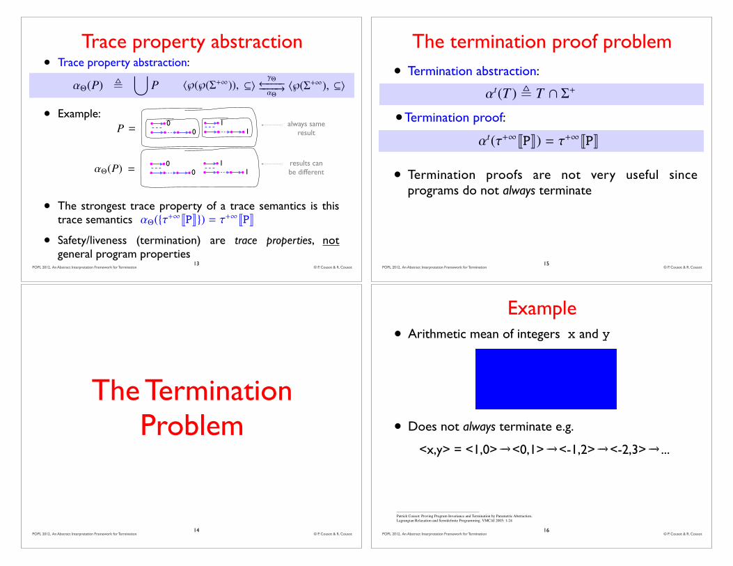
POPL 2012, An Abstract Interpretation Framework for Termination © P. Cousot & R. CousotPOPL 2012, An Abstract Interpretation Framework for Termination © P. Cousot & R. Cousot
Trace property abstraction• Trace property abstraction:
• Example:
• The strongest trace property of a trace semantics is this trace semantics
• Safety/liveness (termination) are trace properties, not general program properties
Fixpoint induction follows immediately as a sound ((=) andcomplete (=)) proof method since for all S 2 A,
lfpva f v S () 9P 2 A : a v P ^ f (P) v P ^ P v S .
S is called a specification or invariant and P is an inductive invariant.The idea is that to prove an invariant S , one has to check (inchecking/verification methods), to guess (in proof methods) or tocompute (in analysis methods) a stronger inductive invariant P.
Following [19, 21], abstraction is formalized by Galois connec-tions7 hA, vi ���! ���↵
�hB, �i between posets hA, vi and hB, �imeaning
that ↵ 2 A 7! B, � 2 B 7! A and 8x 2 A : 8y 2 B : ↵(x) � y ()x v �(y). We write hA, vi ���!�! ����↵
�hB, �i when the abstraction ↵ is
surjective (hence the concretization � is injective), hA, vi ����! ����↵�hB,
�i when ↵ is injective (hence � is surjective), and hA, vi ���!�! ����↵�hB,
�i when ↵ is bijective.Given a concrete fixpoint characterization lfpva f of program
properties on complete lattices or cpos hA, vi with a v f (a) andan abstraction hA, vi ���! ���↵
�hB, �i, the su�cient commutation
condition ↵ � f = f � ↵ (respectively semi-commutation condition↵ � f � f � ↵)8 implies the fixpoint abstraction ↵(lfpva f ) =lfp�↵(a) f (resp. fixpoint approximation ↵(lfpva f ) � lfp�↵(a) f ) [21]. The[semi-]commutation condition can be restricted to the iterates off from a or to the elements of A which are v-less that or equal tolfpva f . The result also holds when ↵ is continuous [13]. In absenceof existence of a best abstraction, similar results can be obtainedusing only one of the abstraction or concretization functions [26].
3. Transition semanticsWe consider a programming language with nondeterministic pro-grams P. The set of all states of P is ⌃JPK. The transition relation⌧JPK 2 }(⌃JPK ⇥ ⌃JPK) describes the possible transitions betweena state and its immediate successor states during program execu-tion [11, 21]. The program small-step operational semantics is thetransition system h⌃JPK, ⌧JPKi. When restricting to initial statesIJPK 2 }(⌃JPK), we write h⌃JPK, IJPK, ⌧JPKi. The termination/block-ing states are �⌧JPK , �
s 2 ⌃JPK | 8s0 2 ⌃JPK : hs, s0i < ⌧JPK . Forbrevity we write X for XJPK e.g. h⌃, ⌧i, h⌃, I, ⌧i, or �⌧.
4. Trace semantics4.1 TracesWe let ⌃n (⌃0 , ;), ⌃+ = S
n2N ⌃n, ⌃⇤ , ⌃+ [ {"}, ⌃1, ⌃+1 ,
⌃+ [ ⌃1, and ⌃⇤1 , ⌃⇤ [ ⌃1 be the set of all finite traces of lengthn 2 N , non-empty finite, finite, infinite, non-empty finite or infinite,and finite or infinite traces over the states ⌃ where " is the emptytrace.
We define the following operations on traces, writing |�| for thelength of the trace � 2 ⌃+1, �[n,m], 0 6 n 6 m for the subtrace�n, �n+1, . . . , �min(m,|�|�1) of �, and ��0 for the concatenation of�,�0 2 ⌃⇤1 (with �" = "� = � and ��0 = � when � 2 ⌃1).
We define the following operations on sets of traces writing Sfor the set of traces {� 2 ⌃1 | �0 2 S } made of one state of S 2 }(⌃)(for example, the termination states �⌧ , {s 2 ⌃ | 8s0 2 ⌃ : hs,s0i < ⌧} can also be understood as traces of length one {� 2 ⌃1 |8s 2 ⌃ : h�0, si < ⌧}), t for the set of traces {� 2 ⌃2 | h�0,�1i 2 t} made of two consecutive states of the relation t 2 }(⌃ ⇥ ⌃),T+ , T \ ⌃+ for the selection of the non-empty finite traces ofT 2 }(⌃⇤1), T1 , T \ ⌃1 for the selection of the infinite traces of
7 [21] also introduced formalizations of abstraction using closure operators,ideals, congruences, etc. and showed all of them to be equivalent to Galoisconnections.8 v is the pointwise extension of a partial order v to maps f v g , 8x :f (x) v g(x).
T , TT 0 , {��0 | � 2 T ^ �0 2 T 0} for the concatenation of sets oftraces, and T # T 0 , {�s�0 | s 2 ⌃ ^ �s 2 T ^ s�0 2 T 0} for thesequencing of sets of traces T,T 0 2 }(⌃⇤1).
4.2 Partial and complete /maximal trace semanticsThe partial trace semantics ⇥+1JPK 2 }(⌃+1JPK) of a program P isa set of non-empty execution traces. In particular, the partial tracesemantics generated by a transition system h⌃, ⌧i is ⌧+1JPK suchthat9
⌧ nJPK ,n
� 2 ⌃n�
�
� 8i 2 [0, n � 1) : h�i, �i+1i 2 ⌧JPK o
, n > 0
⌧1JPK ,n
� 2 ⌃1�
�
� 8i 2 N : h�i, �i+1i 2 ⌧JPK o
⌧+JPK ,[
n>0
⌧ nJPK, ⌧+1JPK , ⌧+JPK [ ⌧1JPK .The complete or maximal trace semantics ⌧nJPK , ↵M(⌧ nJPK),⌧+JPK = ↵M(⌧+JPK) and ⌧+1JPK , ↵M(⌧+1JPK) are obtained by
the abstraction h}(⌃+1), ✓i ����!�! ������↵M
�M
h}(⌃+1), ✓i where
↵M(T ) ,[
n2N
n
� 2 T \ ⌃n�
�
� �n�1 2 �⌧JPK o
[ T1
eliminates those finite partial computations that are not terminated.
4.3 Fixpoint trace semanticsThe partial trace semantics of a program P can be given in fixpointform [28].
⌧+JPK = lfp✓; � � +⌧ JPK = lfp✓;
�!� +⌧ JPK, ⌧1JPK = gfp✓⌃1 �
� 1⌧ JPK
⌧+1JPK = lfp✓; � � +⌧ JPK [ gfp✓⌃1 �
� 1⌧ JPK = lfpv⌃1 �
� +1⌧ JPK
� � +⌧ JPKT , ⌃1 [ ⌧JPK # T �!
� +⌧ JPKT , ⌃1 [ T # ⌧JPK� � 1⌧ JPKT , ⌧JPK # T �
� +1⌧ JPKT , ⌃1 t ⌧JPK # T
where h}(⌃⇤1), v, ⌃1, ⌃⇤, t, ui is a complete lattice for thecomputational order (T1 v T2) , (T+1 ✓ T+2 ) ^ (T11 ◆ T12 ) and(T1 t T2) , (T+1 [ T+2 ) [ (T11 \ T12 ). The fixpoint complete tracesemantics of a program P is calculated by abstraction with ↵M .⌧+1JPK = lfp✓; �
� +⌧ JPK [ gfp✓⌃1 �
� 1⌧ JPK = lfpv⌃1 �
� +1⌧ JPK where
� � +⌧ JPKT , �⌧JPK [ ⌧JPK # T, and � � +1⌧ JPKT , �⌧JPK t ⌧JPK # T .
5. PropertiesFollowing [19, 21], properties are represented by the set of elementswhich have these properties. So the properties of programs whichsemantics are sets of traces in }(⌃+1) are sets of sets of traces in}(}(⌃+1)).
The collecting semantics�
⇥+1JPK 2 }(}(⌃+1)) is the strongestprogram property10 of a program with trace semantics ⇥+1JPK.
The trace property abstraction of program properties is h}(}(⌃+1)),✓i ����! ����↵⇥
�⇥ h}(⌃+1), ✓i such that
↵⇥(P) ,[
P and �⇥(Q) , }(Q) .
The traditional safety/liveness program properties are relativeto the trace property abstraction of the collecting semantics↵⇥
�{⇥+1JPK}� = ⇥+1JPK 2 }(⌃+1).Some program properties are not trace properties [5]. An exam-
ple is “all program executions are deterministic” which is�{�}
�
�
�
9 [n,m] , {n, n + 1, . . . ,m} is the closed interval, ; when m < n, while [n,m) , {n, n + 1, . . . ,m � 1} is left closed and right opened, ; when m 6 n.10 strongest in that the collecting semantics implies all other programproperties (where logical implication A =) B is interpreted as A ✓ B).
00
11
Fixpoint induction follows immediately as a sound ((=) andcomplete (=)) proof method since for all S 2 A,
lfpva f v S () 9P 2 A : a v P ^ f (P) v P ^ P v S .
S is called a specification or invariant and P is an inductive invariant.The idea is that to prove an invariant S , one has to check (inchecking/verification methods), to guess (in proof methods) or tocompute (in analysis methods) a stronger inductive invariant P.
Following [19, 21], abstraction is formalized by Galois connec-tions7 hA, vi ���! ���↵
�hB, �i between posets hA, vi and hB, �imeaning
that ↵ 2 A 7! B, � 2 B 7! A and 8x 2 A : 8y 2 B : ↵(x) � y ()x v �(y). We write hA, vi ���!�! ����↵
�hB, �i when the abstraction ↵ is
surjective (hence the concretization � is injective), hA, vi ����! ����↵�hB,
�i when ↵ is injective (hence � is surjective), and hA, vi ���!�! ����↵�hB,
�i when ↵ is bijective.Given a concrete fixpoint characterization lfpva f of program
properties on complete lattices or cpos hA, vi with a v f (a) andan abstraction hA, vi ���! ���↵
�hB, �i, the su�cient commutation
condition ↵ � f = f � ↵ (respectively semi-commutation condition↵ � f � f � ↵)8 implies the fixpoint abstraction ↵(lfpva f ) =lfp�↵(a) f (resp. fixpoint approximation ↵(lfpva f ) � lfp�↵(a) f ) [21]. The[semi-]commutation condition can be restricted to the iterates off from a or to the elements of A which are v-less that or equal tolfpva f . The result also holds when ↵ is continuous [13]. In absenceof existence of a best abstraction, similar results can be obtainedusing only one of the abstraction or concretization functions [26].
3. Transition semanticsWe consider a programming language with nondeterministic pro-grams P. The set of all states of P is ⌃JPK. The transition relation⌧JPK 2 }(⌃JPK ⇥ ⌃JPK) describes the possible transitions betweena state and its immediate successor states during program execu-tion [11, 21]. The program small-step operational semantics is thetransition system h⌃JPK, ⌧JPKi. When restricting to initial statesIJPK 2 }(⌃JPK), we write h⌃JPK, IJPK, ⌧JPKi. The termination/block-ing states are �⌧JPK , �
s 2 ⌃JPK | 8s0 2 ⌃JPK : hs, s0i < ⌧JPK . Forbrevity we write X for XJPK e.g. h⌃, ⌧i, h⌃, I, ⌧i, or �⌧.
4. Trace semantics4.1 TracesWe let ⌃n (⌃0 , ;), ⌃+ = S
n2N ⌃n, ⌃⇤ , ⌃+ [ {"}, ⌃1, ⌃+1 ,
⌃+ [ ⌃1, and ⌃⇤1 , ⌃⇤ [ ⌃1 be the set of all finite traces of lengthn 2 N , non-empty finite, finite, infinite, non-empty finite or infinite,and finite or infinite traces over the states ⌃ where " is the emptytrace.
We define the following operations on traces, writing |�| for thelength of the trace � 2 ⌃+1, �[n,m], 0 6 n 6 m for the subtrace�n, �n+1, . . . , �min(m,|�|�1) of �, and ��0 for the concatenation of�,�0 2 ⌃⇤1 (with �" = "� = � and ��0 = � when � 2 ⌃1).
We define the following operations on sets of traces writing Sfor the set of traces {� 2 ⌃1 | �0 2 S } made of one state of S 2 }(⌃)(for example, the termination states �⌧ , {s 2 ⌃ | 8s0 2 ⌃ : hs,s0i < ⌧} can also be understood as traces of length one {� 2 ⌃1 |8s 2 ⌃ : h�0, si < ⌧}), t for the set of traces {� 2 ⌃2 | h�0,�1i 2 t} made of two consecutive states of the relation t 2 }(⌃ ⇥ ⌃),T+ , T \ ⌃+ for the selection of the non-empty finite traces ofT 2 }(⌃⇤1), T1 , T \ ⌃1 for the selection of the infinite traces of
7 [21] also introduced formalizations of abstraction using closure operators,ideals, congruences, etc. and showed all of them to be equivalent to Galoisconnections.8 v is the pointwise extension of a partial order v to maps f v g , 8x :f (x) v g(x).
T , TT 0 , {��0 | � 2 T ^ �0 2 T 0} for the concatenation of sets oftraces, and T # T 0 , {�s�0 | s 2 ⌃ ^ �s 2 T ^ s�0 2 T 0} for thesequencing of sets of traces T,T 0 2 }(⌃⇤1).
4.2 Partial and complete /maximal trace semanticsThe partial trace semantics ⇥+1JPK 2 }(⌃+1JPK) of a program P isa set of non-empty execution traces. In particular, the partial tracesemantics generated by a transition system h⌃, ⌧i is ⌧+1JPK suchthat9
⌧ nJPK ,n
� 2 ⌃n�
�
� 8i 2 [0, n � 1) : h�i, �i+1i 2 ⌧JPK o
, n > 0
⌧1JPK ,n
� 2 ⌃1�
�
� 8i 2 N : h�i, �i+1i 2 ⌧JPK o
⌧+JPK ,[
n>0
⌧ nJPK, ⌧+1JPK , ⌧+JPK [ ⌧1JPK .The complete or maximal trace semantics ⌧nJPK , ↵M(⌧ nJPK),⌧+JPK = ↵M(⌧+JPK) and ⌧+1JPK , ↵M(⌧+1JPK) are obtained by
the abstraction h}(⌃+1), ✓i ����!�! ������↵M
�M
h}(⌃+1), ✓i where
↵M(T ) ,[
n2N
n
� 2 T \ ⌃n�
�
� �n�1 2 �⌧JPK o
[ T1
eliminates those finite partial computations that are not terminated.
4.3 Fixpoint trace semanticsThe partial trace semantics of a program P can be given in fixpointform [28].
⌧+JPK = lfp✓; � � +⌧ JPK = lfp✓;
�!� +⌧ JPK, ⌧1JPK = gfp✓⌃1 �
� 1⌧ JPK
⌧+1JPK = lfp✓; � � +⌧ JPK [ gfp✓⌃1 �
� 1⌧ JPK = lfpv⌃1 �
� +1⌧ JPK
� � +⌧ JPKT , ⌃1 [ ⌧JPK # T �!
� +⌧ JPKT , ⌃1 [ T # ⌧JPK� � 1⌧ JPKT , ⌧JPK # T �
� +1⌧ JPKT , ⌃1 t ⌧JPK # T
where h}(⌃⇤1), v, ⌃1, ⌃⇤, t, ui is a complete lattice for thecomputational order (T1 v T2) , (T+1 ✓ T+2 ) ^ (T11 ◆ T12 ) and(T1 t T2) , (T+1 [ T+2 ) [ (T11 \ T12 ). The fixpoint complete tracesemantics of a program P is calculated by abstraction with ↵M .⌧+1JPK = lfp✓; �
� +⌧ JPK [ gfp✓⌃1 �
� 1⌧ JPK = lfpv⌃1 �
� +1⌧ JPK where
� � +⌧ JPKT , �⌧JPK [ ⌧JPK # T, and � � +1⌧ JPKT , �⌧JPK t ⌧JPK # T .
5. PropertiesFollowing [19, 21], properties are represented by the set of elementswhich have these properties. So the properties of programs whichsemantics are sets of traces in }(⌃+1) are sets of sets of traces in}(}(⌃+1)).
The collecting semantics�
⇥+1JPK 2 }(}(⌃+1)) is the strongestprogram property10 of a program with trace semantics ⇥+1JPK.
The trace property abstraction of program properties is h}(}(⌃+1)),✓i ����! ����↵⇥
�⇥ h}(⌃+1), ✓i such that
↵⇥(P) ,[
P and �⇥(Q) , }(Q) .
The traditional safety/liveness program properties are relativeto the trace property abstraction of the collecting semantics↵⇥
�{⇥+1JPK}� = ⇥+1JPK 2 }(⌃+1).Some program properties are not trace properties [5]. An exam-
ple is “all program executions are deterministic” which is�{�}
�
�
�
9 [n,m] , {n, n + 1, . . . ,m} is the closed interval, ; when m < n, while [n,m) , {n, n + 1, . . . ,m � 1} is left closed and right opened, ; when m 6 n.10 strongest in that the collecting semantics implies all other programproperties (where logical implication A =) B is interpreted as A ✓ B).
Fixpoint induction follows immediately as a sound ((=) andcomplete (=)) proof method since for all S 2 A,
lfpva f v S () 9P 2 A : a v P ^ f (P) v P ^ P v S .
S is called a specification or invariant and P is an inductive invariant.The idea is that to prove an invariant S , one has to check (inchecking/verification methods), to guess (in proof methods) or tocompute (in analysis methods) a stronger inductive invariant P.
Following [19, 21], abstraction is formalized by Galois connec-tions7 hA, vi ���! ���↵
�hB, �i between posets hA, vi and hB, �imeaning
that ↵ 2 A 7! B, � 2 B 7! A and 8x 2 A : 8y 2 B : ↵(x) � y ()x v �(y). We write hA, vi ���!�! ����↵
�hB, �i when the abstraction ↵ is
surjective (hence the concretization � is injective), hA, vi ����! ����↵�hB,
�i when ↵ is injective (hence � is surjective), and hA, vi ���!�! ����↵�hB,
�i when ↵ is bijective.Given a concrete fixpoint characterization lfpva f of program
properties on complete lattices or cpos hA, vi with a v f (a) andan abstraction hA, vi ���! ���↵
�hB, �i, the su�cient commutation
condition ↵ � f = f � ↵ (respectively semi-commutation condition↵ � f � f � ↵)8 implies the fixpoint abstraction ↵(lfpva f ) =lfp�↵(a) f (resp. fixpoint approximation ↵(lfpva f ) � lfp�↵(a) f ) [21]. The[semi-]commutation condition can be restricted to the iterates off from a or to the elements of A which are v-less that or equal tolfpva f . The result also holds when ↵ is continuous [13]. In absenceof existence of a best abstraction, similar results can be obtainedusing only one of the abstraction or concretization functions [26].
3. Transition semanticsWe consider a programming language with nondeterministic pro-grams P. The set of all states of P is ⌃JPK. The transition relation⌧JPK 2 }(⌃JPK ⇥ ⌃JPK) describes the possible transitions betweena state and its immediate successor states during program execu-tion [11, 21]. The program small-step operational semantics is thetransition system h⌃JPK, ⌧JPKi. When restricting to initial statesIJPK 2 }(⌃JPK), we write h⌃JPK, IJPK, ⌧JPKi. The termination/block-ing states are �⌧JPK , �
s 2 ⌃JPK | 8s0 2 ⌃JPK : hs, s0i < ⌧JPK . Forbrevity we write X for XJPK e.g. h⌃, ⌧i, h⌃, I, ⌧i, or �⌧.
4. Trace semantics4.1 TracesWe let ⌃n (⌃0 , ;), ⌃+ = S
n2N ⌃n, ⌃⇤ , ⌃+ [ {"}, ⌃1, ⌃+1 ,
⌃+ [ ⌃1, and ⌃⇤1 , ⌃⇤ [ ⌃1 be the set of all finite traces of lengthn 2 N , non-empty finite, finite, infinite, non-empty finite or infinite,and finite or infinite traces over the states ⌃ where " is the emptytrace.
We define the following operations on traces, writing |�| for thelength of the trace � 2 ⌃+1, �[n,m], 0 6 n 6 m for the subtrace�n, �n+1, . . . , �min(m,|�|�1) of �, and ��0 for the concatenation of�,�0 2 ⌃⇤1 (with �" = "� = � and ��0 = � when � 2 ⌃1).
We define the following operations on sets of traces writing Sfor the set of traces {� 2 ⌃1 | �0 2 S } made of one state of S 2 }(⌃)(for example, the termination states �⌧ , {s 2 ⌃ | 8s0 2 ⌃ : hs,s0i < ⌧} can also be understood as traces of length one {� 2 ⌃1 |8s 2 ⌃ : h�0, si < ⌧}), t for the set of traces {� 2 ⌃2 | h�0,�1i 2 t} made of two consecutive states of the relation t 2 }(⌃ ⇥ ⌃),T+ , T \ ⌃+ for the selection of the non-empty finite traces ofT 2 }(⌃⇤1), T1 , T \ ⌃1 for the selection of the infinite traces of
7 [21] also introduced formalizations of abstraction using closure operators,ideals, congruences, etc. and showed all of them to be equivalent to Galoisconnections.8 v is the pointwise extension of a partial order v to maps f v g , 8x :f (x) v g(x).
T , TT 0 , {��0 | � 2 T ^ �0 2 T 0} for the concatenation of sets oftraces, and T # T 0 , {�s�0 | s 2 ⌃ ^ �s 2 T ^ s�0 2 T 0} for thesequencing of sets of traces T,T 0 2 }(⌃⇤1).
4.2 Partial and complete /maximal trace semanticsThe partial trace semantics ⇥+1JPK 2 }(⌃+1JPK) of a program P isa set of non-empty execution traces. In particular, the partial tracesemantics generated by a transition system h⌃, ⌧i is ⌧+1JPK suchthat9
⌧ nJPK ,n
� 2 ⌃n�
�
� 8i 2 [0, n � 1) : h�i, �i+1i 2 ⌧JPK o
, n > 0
⌧1JPK ,n
� 2 ⌃1�
�
� 8i 2 N : h�i, �i+1i 2 ⌧JPK o
⌧+JPK ,[
n>0
⌧ nJPK, ⌧+1JPK , ⌧+JPK [ ⌧1JPK .The complete or maximal trace semantics ⌧nJPK , ↵M(⌧ nJPK),⌧+JPK = ↵M(⌧+JPK) and ⌧+1JPK , ↵M(⌧+1JPK) are obtained by
the abstraction h}(⌃+1), ✓i ����!�! ������↵M
�M
h}(⌃+1), ✓i where
↵M(T ) ,[
n2N
n
� 2 T \ ⌃n�
�
� �n�1 2 �⌧JPK o
[ T1
eliminates those finite partial computations that are not terminated.
4.3 Fixpoint trace semanticsThe partial trace semantics of a program P can be given in fixpointform [28].
⌧+JPK = lfp✓; � � +⌧ JPK = lfp✓;
�!� +⌧ JPK, ⌧1JPK = gfp✓⌃1 �
� 1⌧ JPK
⌧+1JPK = lfp✓; � � +⌧ JPK [ gfp✓⌃1 �
� 1⌧ JPK = lfpv⌃1 �
� +1⌧ JPK
� � +⌧ JPKT , ⌃1 [ ⌧JPK # T �!
� +⌧ JPKT , ⌃1 [ T # ⌧JPK� � 1⌧ JPKT , ⌧JPK # T �
� +1⌧ JPKT , ⌃1 t ⌧JPK # T
where h}(⌃⇤1), v, ⌃1, ⌃⇤, t, ui is a complete lattice for thecomputational order (T1 v T2) , (T+1 ✓ T+2 ) ^ (T11 ◆ T12 ) and(T1 t T2) , (T+1 [ T+2 ) [ (T11 \ T12 ). The fixpoint complete tracesemantics of a program P is calculated by abstraction with ↵M .⌧+1JPK = lfp✓; �
� +⌧ JPK [ gfp✓⌃1 �
� 1⌧ JPK = lfpv⌃1 �
� +1⌧ JPK where
� � +⌧ JPKT , �⌧JPK [ ⌧JPK # T, and � � +1⌧ JPKT , �⌧JPK t ⌧JPK # T .
5. PropertiesFollowing [19, 21], properties are represented by the set of elementswhich have these properties. So the properties of programs whichsemantics are sets of traces in }(⌃+1) are sets of sets of traces in}(}(⌃+1)).
The collecting semantics�
⇥+1JPK 2 }(}(⌃+1)) is the strongestprogram property10 of a program with trace semantics ⇥+1JPK.
The trace property abstraction of program properties is h}(}(⌃+1)),✓i ����! ����↵⇥
�⇥ h}(⌃+1), ✓i such that
↵⇥(P) ,[
P and �⇥(Q) , }(Q) .
The traditional safety/liveness program properties are relativeto the trace property abstraction of the collecting semantics↵⇥
�{⇥+1JPK}� = ⇥+1JPK 2 }(⌃+1).Some program properties are not trace properties [5]. An exam-
ple is “all program executions are deterministic” which is�{�}
�
�
�
9 [n,m] , {n, n + 1, . . . ,m} is the closed interval, ; when m < n, while [n,m) , {n, n + 1, . . . ,m � 1} is left closed and right opened, ; when m 6 n.10 strongest in that the collecting semantics implies all other programproperties (where logical implication A =) B is interpreted as A ✓ B).
Fixpoint induction follows immediately as a sound ((=) andcomplete (=)) proof method since for all S 2 A,
lfpva f v S () 9P 2 A : a v P ^ f (P) v P ^ P v S .
S is called a specification or invariant and P is an inductive invariant.The idea is that to prove an invariant S , one has to check (inchecking/verification methods), to guess (in proof methods) or tocompute (in analysis methods) a stronger inductive invariant P.
Following [19, 21], abstraction is formalized by Galois connec-tions7 hA, vi ���! ���↵
�hB, �i between posets hA, vi and hB, �imeaning
that ↵ 2 A 7! B, � 2 B 7! A and 8x 2 A : 8y 2 B : ↵(x) � y ()x v �(y). We write hA, vi ���!�! ����↵
�hB, �i when the abstraction ↵ is
surjective (hence the concretization � is injective), hA, vi ����! ����↵�hB,
�i when ↵ is injective (hence � is surjective), and hA, vi ���!�! ����↵�hB,
�i when ↵ is bijective.Given a concrete fixpoint characterization lfpva f of program
properties on complete lattices or cpos hA, vi with a v f (a) andan abstraction hA, vi ���! ���↵
�hB, �i, the su�cient commutation
condition ↵ � f = f � ↵ (respectively semi-commutation condition↵ � f � f � ↵)8 implies the fixpoint abstraction ↵(lfpva f ) =lfp�↵(a) f (resp. fixpoint approximation ↵(lfpva f ) � lfp�↵(a) f ) [21]. The[semi-]commutation condition can be restricted to the iterates off from a or to the elements of A which are v-less that or equal tolfpva f . The result also holds when ↵ is continuous [13]. In absenceof existence of a best abstraction, similar results can be obtainedusing only one of the abstraction or concretization functions [26].
3. Transition semanticsWe consider a programming language with nondeterministic pro-grams P. The set of all states of P is ⌃JPK. The transition relation⌧JPK 2 }(⌃JPK ⇥ ⌃JPK) describes the possible transitions betweena state and its immediate successor states during program execu-tion [11, 21]. The program small-step operational semantics is thetransition system h⌃JPK, ⌧JPKi. When restricting to initial statesIJPK 2 }(⌃JPK), we write h⌃JPK, IJPK, ⌧JPKi. The termination/block-ing states are �⌧JPK , �
s 2 ⌃JPK | 8s0 2 ⌃JPK : hs, s0i < ⌧JPK . Forbrevity we write X for XJPK e.g. h⌃, ⌧i, h⌃, I, ⌧i, or �⌧.
4. Trace semantics4.1 TracesWe let ⌃n (⌃0 , ;), ⌃+ = S
n2N ⌃n, ⌃⇤ , ⌃+ [ {"}, ⌃1, ⌃+1 ,
⌃+ [ ⌃1, and ⌃⇤1 , ⌃⇤ [ ⌃1 be the set of all finite traces of lengthn 2 N , non-empty finite, finite, infinite, non-empty finite or infinite,and finite or infinite traces over the states ⌃ where " is the emptytrace.
We define the following operations on traces, writing |�| for thelength of the trace � 2 ⌃+1, �[n,m], 0 6 n 6 m for the subtrace�n, �n+1, . . . , �min(m,|�|�1) of �, and ��0 for the concatenation of�,�0 2 ⌃⇤1 (with �" = "� = � and ��0 = � when � 2 ⌃1).
We define the following operations on sets of traces writing Sfor the set of traces {� 2 ⌃1 | �0 2 S } made of one state of S 2 }(⌃)(for example, the termination states �⌧ , {s 2 ⌃ | 8s0 2 ⌃ : hs,s0i < ⌧} can also be understood as traces of length one {� 2 ⌃1 |8s 2 ⌃ : h�0, si < ⌧}), t for the set of traces {� 2 ⌃2 | h�0,�1i 2 t} made of two consecutive states of the relation t 2 }(⌃ ⇥ ⌃),T+ , T \ ⌃+ for the selection of the non-empty finite traces ofT 2 }(⌃⇤1), T1 , T \ ⌃1 for the selection of the infinite traces of
7 [21] also introduced formalizations of abstraction using closure operators,ideals, congruences, etc. and showed all of them to be equivalent to Galoisconnections.8 v is the pointwise extension of a partial order v to maps f v g , 8x :f (x) v g(x).
T , TT 0 , {��0 | � 2 T ^ �0 2 T 0} for the concatenation of sets oftraces, and T # T 0 , {�s�0 | s 2 ⌃ ^ �s 2 T ^ s�0 2 T 0} for thesequencing of sets of traces T,T 0 2 }(⌃⇤1).
4.2 Partial and complete /maximal trace semanticsThe partial trace semantics ⇥+1JPK 2 }(⌃+1JPK) of a program P isa set of non-empty execution traces. In particular, the partial tracesemantics generated by a transition system h⌃, ⌧i is ⌧+1JPK suchthat9
⌧ nJPK ,n
� 2 ⌃n�
�
� 8i 2 [0, n � 1) : h�i, �i+1i 2 ⌧JPK o
, n > 0
⌧1JPK ,n
� 2 ⌃1�
�
� 8i 2 N : h�i, �i+1i 2 ⌧JPK o
⌧+JPK ,[
n>0
⌧ nJPK, ⌧+1JPK , ⌧+JPK [ ⌧1JPK .The complete or maximal trace semantics ⌧nJPK , ↵M(⌧ nJPK),⌧+JPK = ↵M(⌧+JPK) and ⌧+1JPK , ↵M(⌧+1JPK) are obtained by
the abstraction h}(⌃+1), ✓i ����!�! ������↵M
�M
h}(⌃+1), ✓i where
↵M(T ) ,[
n2N
n
� 2 T \ ⌃n�
�
� �n�1 2 �⌧JPK o
[ T1
eliminates those finite partial computations that are not terminated.
4.3 Fixpoint trace semanticsThe partial trace semantics of a program P can be given in fixpointform [28].
⌧+JPK = lfp✓; � � +⌧ JPK = lfp✓;
�!� +⌧ JPK, ⌧1JPK = gfp✓⌃1 �
� 1⌧ JPK
⌧+1JPK = lfp✓; � � +⌧ JPK [ gfp✓⌃1 �
� 1⌧ JPK = lfpv⌃1 �
� +1⌧ JPK
� � +⌧ JPKT , ⌃1 [ ⌧JPK # T �!
� +⌧ JPKT , ⌃1 [ T # ⌧JPK� � 1⌧ JPKT , ⌧JPK # T �
� +1⌧ JPKT , ⌃1 t ⌧JPK # T
where h}(⌃⇤1), v, ⌃1, ⌃⇤, t, ui is a complete lattice for thecomputational order (T1 v T2) , (T+1 ✓ T+2 ) ^ (T11 ◆ T12 ) and(T1 t T2) , (T+1 [ T+2 ) [ (T11 \ T12 ). The fixpoint complete tracesemantics of a program P is calculated by abstraction with ↵M .⌧+1JPK = lfp✓; �
� +⌧ JPK [ gfp✓⌃1 �
� 1⌧ JPK = lfpv⌃1 �
� +1⌧ JPK where
� � +⌧ JPKT , �⌧JPK [ ⌧JPK # T, and � � +1⌧ JPKT , �⌧JPK t ⌧JPK # T .
5. PropertiesFollowing [19, 21], properties are represented by the set of elementswhich have these properties. So the properties of programs whichsemantics are sets of traces in }(⌃+1) are sets of sets of traces in}(}(⌃+1)).
The collecting semantics�
⇥+1JPK 2 }(}(⌃+1)) is the strongestprogram property10 of a program with trace semantics ⇥+1JPK.
The trace property abstraction of program properties is h}(}(⌃+1)),✓i ����! ����↵⇥
�⇥ h}(⌃+1), ✓i such that
↵⇥(P) ,[
P and �⇥(Q) , }(Q) .
The traditional safety/liveness program properties are relativeto the trace property abstraction of the collecting semantics↵⇥
�{⇥+1JPK}� = ⇥+1JPK 2 }(⌃+1).Some program properties are not trace properties [5]. An exam-
ple is “all program executions are deterministic” which is�{�}
�
�
�
9 [n,m] , {n, n + 1, . . . ,m} is the closed interval, ; when m < n, while [n,m) , {n, n + 1, . . . ,m � 1} is left closed and right opened, ; when m 6 n.10 strongest in that the collecting semantics implies all other programproperties (where logical implication A =) B is interpreted as A ✓ B).
00
11
Fixpoint induction follows immediately as a sound ((=) andcomplete (=)) proof method since for all S 2 A,
lfpva f v S () 9P 2 A : a v P ^ f (P) v P ^ P v S .
S is called a specification or invariant and P is an inductive invariant.The idea is that to prove an invariant S , one has to check (inchecking/verification methods), to guess (in proof methods) or tocompute (in analysis methods) a stronger inductive invariant P.
Following [19, 21], abstraction is formalized by Galois connec-tions7 hA, vi ���! ���↵
�hB, �i between posets hA, vi and hB, �imeaning
that ↵ 2 A 7! B, � 2 B 7! A and 8x 2 A : 8y 2 B : ↵(x) � y ()x v �(y). We write hA, vi ���!�! ����↵
�hB, �i when the abstraction ↵ is
surjective (hence the concretization � is injective), hA, vi ����! ����↵�hB,
�i when ↵ is injective (hence � is surjective), and hA, vi ���!�! ����↵�hB,
�i when ↵ is bijective.Given a concrete fixpoint characterization lfpva f of program
properties on complete lattices or cpos hA, vi with a v f (a) andan abstraction hA, vi ���! ���↵
�hB, �i, the su�cient commutation
condition ↵ � f = f � ↵ (respectively semi-commutation condition↵ � f � f � ↵)8 implies the fixpoint abstraction ↵(lfpva f ) =lfp�↵(a) f (resp. fixpoint approximation ↵(lfpva f ) � lfp�↵(a) f ) [21]. The[semi-]commutation condition can be restricted to the iterates off from a or to the elements of A which are v-less that or equal tolfpva f . The result also holds when ↵ is continuous [13]. In absenceof existence of a best abstraction, similar results can be obtainedusing only one of the abstraction or concretization functions [26].
3. Transition semanticsWe consider a programming language with nondeterministic pro-grams P. The set of all states of P is ⌃JPK. The transition relation⌧JPK 2 }(⌃JPK ⇥ ⌃JPK) describes the possible transitions betweena state and its immediate successor states during program execu-tion [11, 21]. The program small-step operational semantics is thetransition system h⌃JPK, ⌧JPKi. When restricting to initial statesIJPK 2 }(⌃JPK), we write h⌃JPK, IJPK, ⌧JPKi. The termination/block-ing states are �⌧JPK , �
s 2 ⌃JPK | 8s0 2 ⌃JPK : hs, s0i < ⌧JPK . Forbrevity we write X for XJPK e.g. h⌃, ⌧i, h⌃, I, ⌧i, or �⌧.
4. Trace semantics4.1 TracesWe let ⌃n (⌃0 , ;), ⌃+ = S
n2N ⌃n, ⌃⇤ , ⌃+ [ {"}, ⌃1, ⌃+1 ,
⌃+ [ ⌃1, and ⌃⇤1 , ⌃⇤ [ ⌃1 be the set of all finite traces of lengthn 2 N , non-empty finite, finite, infinite, non-empty finite or infinite,and finite or infinite traces over the states ⌃ where " is the emptytrace.
We define the following operations on traces, writing |�| for thelength of the trace � 2 ⌃+1, �[n,m], 0 6 n 6 m for the subtrace�n, �n+1, . . . , �min(m,|�|�1) of �, and ��0 for the concatenation of�,�0 2 ⌃⇤1 (with �" = "� = � and ��0 = � when � 2 ⌃1).
We define the following operations on sets of traces writing Sfor the set of traces {� 2 ⌃1 | �0 2 S } made of one state of S 2 }(⌃)(for example, the termination states �⌧ , {s 2 ⌃ | 8s0 2 ⌃ : hs,s0i < ⌧} can also be understood as traces of length one {� 2 ⌃1 |8s 2 ⌃ : h�0, si < ⌧}), t for the set of traces {� 2 ⌃2 | h�0,�1i 2 t} made of two consecutive states of the relation t 2 }(⌃ ⇥ ⌃),T+ , T \ ⌃+ for the selection of the non-empty finite traces ofT 2 }(⌃⇤1), T1 , T \ ⌃1 for the selection of the infinite traces of
7 [21] also introduced formalizations of abstraction using closure operators,ideals, congruences, etc. and showed all of them to be equivalent to Galoisconnections.8 v is the pointwise extension of a partial order v to maps f v g , 8x :f (x) v g(x).
T , TT 0 , {��0 | � 2 T ^ �0 2 T 0} for the concatenation of sets oftraces, and T # T 0 , {�s�0 | s 2 ⌃ ^ �s 2 T ^ s�0 2 T 0} for thesequencing of sets of traces T,T 0 2 }(⌃⇤1).
4.2 Partial and complete /maximal trace semanticsThe partial trace semantics ⇥+1JPK 2 }(⌃+1JPK) of a program P isa set of non-empty execution traces. In particular, the partial tracesemantics generated by a transition system h⌃, ⌧i is ⌧+1JPK suchthat9
⌧ nJPK ,n
� 2 ⌃n�
�
� 8i 2 [0, n � 1) : h�i, �i+1i 2 ⌧JPK o
, n > 0
⌧1JPK ,n
� 2 ⌃1�
�
� 8i 2 N : h�i, �i+1i 2 ⌧JPK o
⌧+JPK ,[
n>0
⌧ nJPK, ⌧+1JPK , ⌧+JPK [ ⌧1JPK .The complete or maximal trace semantics ⌧nJPK , ↵M(⌧ nJPK),⌧+JPK = ↵M(⌧+JPK) and ⌧+1JPK , ↵M(⌧+1JPK) are obtained by
the abstraction h}(⌃+1), ✓i ����!�! ������↵M
�M
h}(⌃+1), ✓i where
↵M(T ) ,[
n2N
n
� 2 T \ ⌃n�
�
� �n�1 2 �⌧JPK o
[ T1
eliminates those finite partial computations that are not terminated.
4.3 Fixpoint trace semanticsThe partial trace semantics of a program P can be given in fixpointform [28].
⌧+JPK = lfp✓; � � +⌧ JPK = lfp✓;
�!� +⌧ JPK, ⌧1JPK = gfp✓⌃1 �
� 1⌧ JPK
⌧+1JPK = lfp✓; � � +⌧ JPK [ gfp✓⌃1 �
� 1⌧ JPK = lfpv⌃1 �
� +1⌧ JPK
� � +⌧ JPKT , ⌃1 [ ⌧JPK # T �!
� +⌧ JPKT , ⌃1 [ T # ⌧JPK� � 1⌧ JPKT , ⌧JPK # T �
� +1⌧ JPKT , ⌃1 t ⌧JPK # T
where h}(⌃⇤1), v, ⌃1, ⌃⇤, t, ui is a complete lattice for thecomputational order (T1 v T2) , (T+1 ✓ T+2 ) ^ (T11 ◆ T12 ) and(T1 t T2) , (T+1 [ T+2 ) [ (T11 \ T12 ). The fixpoint complete tracesemantics of a program P is calculated by abstraction with ↵M .⌧+1JPK = lfp✓; �
� +⌧ JPK [ gfp✓⌃1 �
� 1⌧ JPK = lfpv⌃1 �
� +1⌧ JPK where
� � +⌧ JPKT , �⌧JPK [ ⌧JPK # T, and � � +1⌧ JPKT , �⌧JPK t ⌧JPK # T .
5. PropertiesFollowing [19, 21], properties are represented by the set of elementswhich have these properties. So the properties of programs whichsemantics are sets of traces in }(⌃+1) are sets of sets of traces in}(}(⌃+1)).
The collecting semantics�
⇥+1JPK 2 }(}(⌃+1)) is the strongestprogram property10 of a program with trace semantics ⇥+1JPK.
The trace property abstraction of program properties is h}(}(⌃+1)),✓i ����! ����↵⇥
�⇥ h}(⌃+1), ✓i such that
↵⇥(P) ,[
P and �⇥(Q) , }(Q) .
The traditional safety/liveness program properties are relativeto the trace property abstraction of the collecting semantics↵⇥
�{⇥+1JPK}� = ⇥+1JPK 2 }(⌃+1).Some program properties are not trace properties [5]. An exam-
ple is “all program executions are deterministic” which is�{�}
�
�
�
9 [n,m] , {n, n + 1, . . . ,m} is the closed interval, ; when m < n, while [n,m) , {n, n + 1, . . . ,m � 1} is left closed and right opened, ; when m 6 n.10 strongest in that the collecting semantics implies all other programproperties (where logical implication A =) B is interpreted as A ✓ B).
Fixpoint induction follows immediately as a sound ((=) andcomplete (=)) proof method since for all S 2 A,
lfpva f v S () 9P 2 A : a v P ^ f (P) v P ^ P v S .
S is called a specification or invariant and P is an inductive invariant.The idea is that to prove an invariant S , one has to check (inchecking/verification methods), to guess (in proof methods) or tocompute (in analysis methods) a stronger inductive invariant P.
Following [19, 21], abstraction is formalized by Galois connec-tions7 hA, vi ���! ���↵
�hB, �i between posets hA, vi and hB, �imeaning
that ↵ 2 A 7! B, � 2 B 7! A and 8x 2 A : 8y 2 B : ↵(x) � y ()x v �(y). We write hA, vi ���!�! ����↵
�hB, �i when the abstraction ↵ is
surjective (hence the concretization � is injective), hA, vi ����! ����↵�hB,
�i when ↵ is injective (hence � is surjective), and hA, vi ���!�! ����↵�hB,
�i when ↵ is bijective.Given a concrete fixpoint characterization lfpva f of program
properties on complete lattices or cpos hA, vi with a v f (a) andan abstraction hA, vi ���! ���↵
�hB, �i, the su�cient commutation
condition ↵ � f = f � ↵ (respectively semi-commutation condition↵ � f � f � ↵)8 implies the fixpoint abstraction ↵(lfpva f ) =lfp�↵(a) f (resp. fixpoint approximation ↵(lfpva f ) � lfp�↵(a) f ) [21]. The[semi-]commutation condition can be restricted to the iterates off from a or to the elements of A which are v-less that or equal tolfpva f . The result also holds when ↵ is continuous [13]. In absenceof existence of a best abstraction, similar results can be obtainedusing only one of the abstraction or concretization functions [26].
3. Transition semanticsWe consider a programming language with nondeterministic pro-grams P. The set of all states of P is ⌃JPK. The transition relation⌧JPK 2 }(⌃JPK ⇥ ⌃JPK) describes the possible transitions betweena state and its immediate successor states during program execu-tion [11, 21]. The program small-step operational semantics is thetransition system h⌃JPK, ⌧JPKi. When restricting to initial statesIJPK 2 }(⌃JPK), we write h⌃JPK, IJPK, ⌧JPKi. The termination/block-ing states are �⌧JPK , �
s 2 ⌃JPK | 8s0 2 ⌃JPK : hs, s0i < ⌧JPK . Forbrevity we write X for XJPK e.g. h⌃, ⌧i, h⌃, I, ⌧i, or �⌧.
4. Trace semantics4.1 TracesWe let ⌃n (⌃0 , ;), ⌃+ = S
n2N ⌃n, ⌃⇤ , ⌃+ [ {"}, ⌃1, ⌃+1 ,
⌃+ [ ⌃1, and ⌃⇤1 , ⌃⇤ [ ⌃1 be the set of all finite traces of lengthn 2 N , non-empty finite, finite, infinite, non-empty finite or infinite,and finite or infinite traces over the states ⌃ where " is the emptytrace.
We define the following operations on traces, writing |�| for thelength of the trace � 2 ⌃+1, �[n,m], 0 6 n 6 m for the subtrace�n, �n+1, . . . , �min(m,|�|�1) of �, and ��0 for the concatenation of�,�0 2 ⌃⇤1 (with �" = "� = � and ��0 = � when � 2 ⌃1).
We define the following operations on sets of traces writing Sfor the set of traces {� 2 ⌃1 | �0 2 S } made of one state of S 2 }(⌃)(for example, the termination states �⌧ , {s 2 ⌃ | 8s0 2 ⌃ : hs,s0i < ⌧} can also be understood as traces of length one {� 2 ⌃1 |8s 2 ⌃ : h�0, si < ⌧}), t for the set of traces {� 2 ⌃2 | h�0,�1i 2 t} made of two consecutive states of the relation t 2 }(⌃ ⇥ ⌃),T+ , T \ ⌃+ for the selection of the non-empty finite traces ofT 2 }(⌃⇤1), T1 , T \ ⌃1 for the selection of the infinite traces of
7 [21] also introduced formalizations of abstraction using closure operators,ideals, congruences, etc. and showed all of them to be equivalent to Galoisconnections.8 v is the pointwise extension of a partial order v to maps f v g , 8x :f (x) v g(x).
T , TT 0 , {��0 | � 2 T ^ �0 2 T 0} for the concatenation of sets oftraces, and T # T 0 , {�s�0 | s 2 ⌃ ^ �s 2 T ^ s�0 2 T 0} for thesequencing of sets of traces T,T 0 2 }(⌃⇤1).
4.2 Partial and complete /maximal trace semanticsThe partial trace semantics ⇥+1JPK 2 }(⌃+1JPK) of a program P isa set of non-empty execution traces. In particular, the partial tracesemantics generated by a transition system h⌃, ⌧i is ⌧+1JPK suchthat9
⌧ nJPK ,n
� 2 ⌃n�
�
� 8i 2 [0, n � 1) : h�i, �i+1i 2 ⌧JPK o
, n > 0
⌧1JPK ,n
� 2 ⌃1�
�
� 8i 2 N : h�i, �i+1i 2 ⌧JPK o
⌧+JPK ,[
n>0
⌧ nJPK, ⌧+1JPK , ⌧+JPK [ ⌧1JPK .The complete or maximal trace semantics ⌧nJPK , ↵M(⌧ nJPK),⌧+JPK = ↵M(⌧+JPK) and ⌧+1JPK , ↵M(⌧+1JPK) are obtained by
the abstraction h}(⌃+1), ✓i ����!�! ������↵M
�M
h}(⌃+1), ✓i where
↵M(T ) ,[
n2N
n
� 2 T \ ⌃n�
�
� �n�1 2 �⌧JPK o
[ T1
eliminates those finite partial computations that are not terminated.
4.3 Fixpoint trace semanticsThe partial trace semantics of a program P can be given in fixpointform [28].
⌧+JPK = lfp✓; � � +⌧ JPK = lfp✓;
�!� +⌧ JPK, ⌧1JPK = gfp✓⌃1 �
� 1⌧ JPK
⌧+1JPK = lfp✓; � � +⌧ JPK [ gfp✓⌃1 �
� 1⌧ JPK = lfpv⌃1 �
� +1⌧ JPK
� � +⌧ JPKT , ⌃1 [ ⌧JPK # T �!
� +⌧ JPKT , ⌃1 [ T # ⌧JPK� � 1⌧ JPKT , ⌧JPK # T �
� +1⌧ JPKT , ⌃1 t ⌧JPK # T
where h}(⌃⇤1), v, ⌃1, ⌃⇤, t, ui is a complete lattice for thecomputational order (T1 v T2) , (T+1 ✓ T+2 ) ^ (T11 ◆ T12 ) and(T1 t T2) , (T+1 [ T+2 ) [ (T11 \ T12 ). The fixpoint complete tracesemantics of a program P is calculated by abstraction with ↵M .⌧+1JPK = lfp✓; �
� +⌧ JPK [ gfp✓⌃1 �
� 1⌧ JPK = lfpv⌃1 �
� +1⌧ JPK where
� � +⌧ JPKT , �⌧JPK [ ⌧JPK # T, and � � +1⌧ JPKT , �⌧JPK t ⌧JPK # T .
5. PropertiesFollowing [19, 21], properties are represented by the set of elementswhich have these properties. So the properties of programs whichsemantics are sets of traces in }(⌃+1) are sets of sets of traces in}(}(⌃+1)).
The collecting semantics�
⇥+1JPK 2 }(}(⌃+1)) is the strongestprogram property10 of a program with trace semantics ⇥+1JPK.
The trace property abstraction of program properties is h}(}(⌃+1)),✓i ����! ����↵⇥
�⇥ h}(⌃+1), ✓i such that
↵⇥(P) ,[
P and �⇥(Q) , }(Q) .
The traditional safety/liveness program properties are relativeto the trace property abstraction of the collecting semantics↵⇥
�{⇥+1JPK}� = ⇥+1JPK 2 }(⌃+1).Some program properties are not trace properties [5]. An exam-
ple is “all program executions are deterministic” which is�{�}
�
�
�
9 [n,m] , {n, n + 1, . . . ,m} is the closed interval, ; when m < n, while [n,m) , {n, n + 1, . . . ,m � 1} is left closed and right opened, ; when m 6 n.10 strongest in that the collecting semantics implies all other programproperties (where logical implication A =) B is interpreted as A ✓ B).
13
↵t(T ) , T \ ⌃+JPKP
↵t(⌧+1JPK) = ⌧+1JPKx � y
x > y
=)
()
↵rk
;
!
↵A
↵G
f1 vv f2
↵rk 2 }(⌃ ⇥ ⌃) 7! (⌃ 67! O)↵rk(r)s , 0 when 8s0 2 ⌃ : hs, s0i < r
↵rk(r)s , supn
↵rk(r)s0 + 1�
�
� 9s0 2 ⌃ : hs, s0i 2 r ^8s0 2 ⌃ : hs, s0i 2 r =) s0 2 dom(↵rk(r))
o
9k : ⌫(x, y) = k, x � y � 2k = 0, k > 0
k = ⌫(x, y)
↵⇥({⌧+1JPK}) = ⌧+1JPK
always sameresult
results canbe different
POPL 2012, An Abstract Interpretation Framework for Termination © P. Cousot & R. CousotPOPL 2012, An Abstract Interpretation Framework for Termination © P. Cousot & R. Cousot
The Termination Problem
14
POPL 2012, An Abstract Interpretation Framework for Termination © P. Cousot & R. Cousot
↵t(T ) , T \ ⌃+JPKP
↵t(⌧+1JPK) = ⌧+1JPK
• Termination abstraction:
•Termination proof:
• Termination proofs are not very useful since programs do not always terminate
POPL 2012, An Abstract Interpretation Framework for Termination © P. Cousot & R. Cousot
The termination proof problem
↵t(T ) , T \ ⌃+JPKP
↵t(⌧+1JPK) = ⌧+1JPK
15
POPL 2012, An Abstract Interpretation Framework for Termination © P. Cousot & R. CousotPOPL 2012, An Abstract Interpretation Framework for Termination © P. Cousot & R. Cousot
Example• Arithmetic mean of integers x and y
• Does not always terminate e.g.
<x,y> = <1,0> <0,1> <-1,2> <-2,3> ...
16
⌧mtJPK , ↵mt(⌧+1JPK) potential termination semantics
while the definite termination collecting semantics of a program Pis defined as
⌧MtJPK , ↵Mt(⌧+1JPK) definite termination semantics.8.4 Fixpoint termination trace semanticsBy abstraction of the fixpoint trace semantics of Sect. 4.3, thestrongest termination property of a program P with operationalsemantics h⌃JPK, ⌧JPKi and termination states �⌧JPK is
⌧mtJPK = lfp✓; � � mt⌧ JPK potential termination
� � mt⌧ JPKT , �⌧JPK [ ⌧JPK # T⌧MtJPK = lfp✓; �
� Mt⌧ JPK definite termination
� � Mt⌧ JPKT , �⌧JPK [ (⌧JPK # T \ ¬(⌧JPK # ¬T ))
where the term ¬(⌧JPK #¬T ) eliminates potential transitions towardsnon-terminating executions.8.5 Proofs in the termination trace domainFixpoint induction provides formal methods to check fixpointover-approximations, either ⌧mtJPK ✓ S or ⌧MtJPK ✓ S . Over-approximations yield necessary but not su�cient termination con-ditions which may introduce spurious infinite traces for which theproof cannot be done. The proof method is therefore useful to proveinvariance under termination assumptions19 but not for may/musttermination.
On the contrary, termination proofs require fixpoint under-approximations S ✓ ⌧mtJPK or S ✓ ⌧MtJPK. Under-approximationsyield su�cient but not necessary termination conditions and so mayeliminate some termination cases for which the termination proofcould have been done automatically. Fixpoint under-approximationproof methods have been proposed e.g. by [15, Sect. 11] and wouldyield the requested termination proof methods. More classically, wewill favor over-approximations for static analysis.
9. Termination domainPrograms may not always potentially/definitely terminate in allstates. So one problem is to determine for which states I 2 }(⌃) doexecutions starting from these states may/must terminate.9.1 Termination domain abstractionThis potential/definite termination domain semantics is provided bythe weakest precondition abstraction h}(⌃+1), ✓i ����! ����
↵w
�w
h}(⌃), ✓iof the termination trace semantics, such that
↵w(T ) , {�0 | � 2 T } precondition abstraction.
9.2 Termination domain semantics⌧wmtJPK , ↵w(⌧mtJPK) potential termination⌧wMtJPK , ↵w(⌧MtJPK) definite termination.
Using Dijkstra’s notations [37], ⌧wmtJPK = wlpJPKtrue and ⌧wMtJPK =wpJPKtrue.
9.3 Fixpoint termination domain semanticsBy fixpoint abstraction of the termination trace semantics in Sect. 8.4using transformer commutation, we get Dijkstra’s fixpoint weakest(liberal) termination precondition semantics [38]20
19 e.g. for Ex. 1, {b, e, l} is invariant, {b, e} is invariant under potentialtermination hypothesis, and {e} is invariant under definite terminationhypothesis.20 The pre-image of Y 2 }(A) by a relation r 2 }(A ⇥ B) is r�1[Y] , {x |9y 2 Y : hx, yi 2 r} also written pre[r]Y while ¬r�1[¬Y] , {x | 8y : y 2Y =) hx, yi 2 r} is gpre[r]Y .
⌧wmtJPK = lfp✓;�!� wmt⌧ JPK weakest liberal termin. precond.
�!� wmt⌧ JPK(R) , �⌧JPK [ ⌧JPK�1[R]
⌧wMtJPK = lfp✓;�!� wMt⌧ JPK weakest termination precondition
�!� wMt⌧ JPK(R) , �⌧JPK [ (⌧JPK�1[R] \ ¬⌧JPK�1[¬R]) .
9.4 Proof and static analysis in the termination domainAs was the case in Sect. 8.5, fixpoint induction is useful for over-approximations, which can be automatically inferred by static analy-sis [11, 12]. On the contrary, termination proofs require under-approximations [15, Sect. 11] proof methods. Although static under-approximation analysis is possible (e.g. [34]), this is not the termi-nation proof technique which is used in practice [38].
10. Termination proofs for the trace semanticsgenerated by a transition system
In practice a termination proof is decomposed in two parts. Firsta necessary termination condition is found by over-approximating⌧wmtJPK or ⌧wMtJPK. Then this necessary termination condition isshown to be su�cient by Floyd/Turing variant function method(e.g. [17]) or inversely (e.g. [8]). This corresponds to di↵erentabstractions, specific to the trace semantics generated by a transitionsystem, that we now elaborate.
10.1 Transition-based termination proofsA program which trace semantics is generated by a transition systemh⌃, ⌧i definitely terminates if and only if the program transitionrelation is well-founded21.
⌧+1JPK ✓ ⌃+JPK () h⌃, ⌧i is well-founded.
In practice one considers traces starting from initial states I 2 }(⌃),e.g. I is the termination domain of Sect. 9. In that case a programwhich trace semantics is generated by a transition system h⌃, ⌧idefinitely terminates for traces starting from initial states I 2 }(⌃)if and only if the program transition relation restricted to reachablestates is well-founded.
↵i(I)(⌧+1JPK) ✓ ⌃+JPK () h↵r(↵i(I)(⌧+1JPK)), ⌧i is well-founded
where the initialization abstraction h}(⌃+1), ✓i �����! �����↵i(I)
�i(I)h}(⌃+1),
✓i is↵i 2 }(⌃) 7! (⌃+1 7! ⌃+1) initialization abstraction
↵i(I)T , �
� 2 T | �0 2 I
and the reachable states abstraction h}(⌃+1), ✓i ����! ����↵r
�r
h}(⌃), ✓iis↵r(T ) , �
s | 9� 2 ⌃⇤,�0 2 ⌃⇤1 : �s�0 2 T
reachabilityabstraction.
The transition-based termination proof method is sound and com-plete. As noticed in Sect. 9, the precondition I can be inferred au-tomatically by static analysis. Moreover, an over-approximationR ◆ ↵r(↵i(I)(⌧+1JPK)) = ⌧JPK⇤[I] 22 of the reachable states can becomputed by classical abstract interpretation algorithms [19].
21 A relation � 2 }(W ⇥W) on a setW is well-founded if and only if thereis no strictly decreasing infinite chain x0 � x1 � . . . � xn � xn+1 � . . . ofelements x0, x1, . . . , xn, xn+1, . . . ofW. hW, �i is called a well-founded set.A (total) well-order is well-founded (total) strict order relation �. The set ofall well-founded relations in }(W ⇥W) is writtenWf(W ⇥W).22 t⇤ is the reflexive transitive closure of a binary relation t.
while (x <> y) { x := x - 1; y := y + 1}
Patrick Cousot: Proving Program Invariance and Termination by Parametric Abstraction, Lagrangian Relaxation and Semidefinite Programming. VMCAI 2005: 1-24

POPL 2012, An Abstract Interpretation Framework for Termination © P. Cousot & R. Cousot
• Determine a necessary condition for program termination and prove it sufficient
• Example:
• (1) Under which necessary conditions
does terminate?
• (2) Prove these conditions to be sufficient
while (x <> y) { x := x - 1; y := y + 1}
POPL 2012, An Abstract Interpretation Framework for Termination © P. Cousot & R. Cousot
The termination inference problem
17
POPL 2012, An Abstract Interpretation Framework for Termination © P. Cousot & R. Cousot
The Termination Inference Problem
18
POPL 2012, An Abstract Interpretation Framework for Termination © P. Cousot & R. CousotPOPL 2012, An Abstract Interpretation Framework for Termination © P. Cousot & R. Cousot
Potential termination• For non-deterministic programs, we may be
interested in potential termination
mayterminate
19
POPL 2012, An Abstract Interpretation Framework for Termination © P. Cousot & R. CousotPOPL 2012, An Abstract Interpretation Framework for Termination © P. Cousot & R. Cousot
Definite termination abstraction• or in definite termination
• Potential and definite termination coincide for deterministic programs. Only definite termination in this presentation.
mustterminate
20

POPL 2012, An Abstract Interpretation Framework for Termination © P. Cousot & R. CousotPOPL 2012, An Abstract Interpretation Framework for Termination © P. Cousot & R. Cousot
Definite termination trace abstraction• Prefix Abstraction
• Definite termination abstraction
� 2 ⌃+1 2 }(}(⌃+1)) 11. The corresponding trace property abstrac-tion is ↵⇥(
�{�}�
�
� � 2 ⌃+1
) = ⌃+1 2 }(⌃+1) which would allowany non-deterministic behavior so that determinism in the concretedomain }(}(⌃+1)) is completely lost in the abstract domain }(⌃+1).
For safety and termination and from now on, we only have toconsider trace properties, which form a complete Boolean latticeh}(⌃+1), ✓, ;, ⌃+1, [, \, ¬i where the partial order ✓ is logicalimplication and the complement is ¬X , ⌃+1 \ X 12.
6. Safety trace semanticsWe now illustrate the classical abstract interpretation framework bygeneralizing invariance verification and static analysis to arbitrarysafety properties. Safety properties are abstractions of program traceproperties (essentially forgetting about liveness properties).6.1 Safety abstractionThe prefix abstraction of a set T of traces is the topological closure13
pf(�) , �
�0 2 ⌃+1�
�
� 9�00 2 ⌃⇤1 : � = �0�00
pf(T ) ,[
�
pf(�)�
�
� � 2 T
.
The prefix abstraction expresses the fact that program executionscan only be observed for a finite period of time (8T : " < pf(T )).
The limit abstraction of a set of traces is the topological closure
lm(T ) , T [ �
� 2 ⌃1 | 8n 2 N : �[0, n] 2 T
.
The limit abstraction expresses the fact that when observing programexecutions for finite periods of time it is impossible to distinguishbetween non-terminating and unbounded finite executions.
The safety abstraction of a set of traces is the topological closuresf , lm � pf = pf � lm � pf .
The safety abstraction provides the strongest program propertyresulting from finite observations of program executions (excludingthe observation of infinite executions).
(Topological) closures ⇢ 2 A 7! A on a poset hA, 6i are abstrac-tions14 hA, 6i ����!�! �����
⇢
1A h⇢[A], 6i.6.2 Safety trace propertiesThe safety trace properties are
SF , sf[}(⌃+1)] =�
sf(P) | P 2}(⌃+1)
=�
P 2}(⌃+1) | sf(P) = P
.
We have the Galois isomorphism
hSF, ✓i ����!�! �����pf+
lm hpf+[}(⌃+)], ✓i
where pf+(T ) = pf(T )+ and so safety trace properties can equiva-lently be represented by their finite prefixes in Sect. 6.4 and 6.5.6.3 Safety semanticsThe safety semantics of a program P is its strongest safety property
⌧sfJPK , sf(⌧+1JPK) ' pf+ � sf(⌧+1JPK) .
6.4 Fixpoint safety semanticsIt follows, by fixpoint abstraction, that the safety semantics of aprogram P with operational semantics h⌃, ⌧i is
11 Assuming inputs, if any, to be part of the states.12 X \ Y , {x 2 X | x < Y} is the set di↵erence.13 A topological closure on a poset hA, 6, _i with partial-order 6 and lub_, if any, is a map ⇢ 2 A 7! A which is extensive 8x 2 A : x 6 ⇢(x),idempotent 8x 2 A : ⇢(⇢(x)) = ⇢(x), and finite lub-preserving 8x, y 2 A :⇢(x_y) = ⇢(x)_⇢(y). This implies that ⇢ is increasing. A closure is extensive,idempotent, and increasing.14 1A is the identity map (respectively relation) on the set A mapping anyelement x 2 A to itself 1A(x) = x (resp. 1A , {hx, xi | x 2 A}).
⌧sfJPK = lfp✓;�!� sf⌧ JPK = lfp✓; �
� sf⌧ JPK where
�!� sf⌧ JPKT , ⌃1 [ T # ⌧JPK forward trace transformer
� � sf⌧ JPKT , ⌃1 [ ⌧JPK # T backward trace transformer.
6.5 Proofs in the safety trace domainBy fixpoint induction, one immediately gets new forward andbackward sound and complete safety proof methods15 generalizinginvariance [37, 40, 48, 49]. For all safety specifications S 2 SF,⌧sfJPK ✓ S () 9P 2 SF : ⌃1 ✓ P ^ ⌧JPK # P ✓ P ^ P ✓ S
() 9P 2 SF : ⌃1 ✓ P ^ P # ⌧JPK ✓ P ^ P ✓ S .Observe that forward and backward safety semantics and proofmethods are respectively equivalent. This property is preserved byrelational abstractions in next Sect. 7, but this is not the generalcase (e.g. with abstractions of Sect. 7.6). [42] is an example of staticanalysis in the safety trace domain.
7. Invariance / reachability semanticsInvariance/reachability is an abstraction of safety and so invarianceproof methods are abstractions of safety proof methods.
7.1 Relational abstraction
The relational abstraction hSF, ✓i ����!�! �����↵R
�R
h}(⌃ ⇥ ⌃), ✓i such that
↵R(T ) , � h�0, �n�1i | n > 0 ^ � 2 ⌃n \ T
(1)�R(R) , �
� 2 ⌃n | n > 0 ^ h�0, �n�1i 2 R
abstracts traces by a relation between their initial and final states (sothat intermediate computations are lost in that abstraction).
7.2 Relational invariance / reachability abstractionApplied to a safety semantics which is prefix-closed, the relationalabstraction provides a relation between initial and current states(where, in particular, “initial” can be any state).
The abstraction ↵R � sf is therefore equal to the relational
reachability abstraction h}(⌃+1), ✓i �����!�! ������↵R⇤
�R⇤
h}(⌃ ⇥ ⌃), ✓i such
that↵R⇤ (T ) , � h�0, �ii | 9n : 0 6 i < n ^ � 2 ⌃n \ T
�R⇤ (R) , �
� 2 ⌃n | n > 0 ^ 8i 2 [0, n) : h�0, �ii 2 R
abstract traces by a relation between their initial and current states.
7.3 Relational invariance / reachability semanticsThe relational invariance/reachability semantics of a program P isits strongest relational reachability property
⌧RJPK , ↵R(⌧+1JPK)
⌧R⇤JPK , ↵R(⌧+1JPK) = ↵R⇤ (⌧+1JPK) = ↵R(⌧sfJPK) = ↵R⇤ (⌧sfJPK) .
7.4 Fixpoint relational invariance / reachability semanticsThe commutation condition applied to the transformer of the safetysemantics ⌧sfJPK yields the fixpoint characterization of the relationalreachability semantics of a program P with operational semanticsh⌃, ⌧i
⌧R⇤JPK = lfp✓;�!� R⇤⌧ JPK = lfp✓; �
� R⇤⌧ JPK
where16
15 In case a temporal logic is used for expressing the inductive safety invariant,this is relative completeness subject to an expressivity hypothesis of thetemporal logic ensuring P 2 SF to be expressible in the logic, see e.g. [10].16 The post-image (or right-image) of X 2 }(A) by a relation r 2 }(A ⇥ B) isr[X] , {y | 9x 2 X : hx, yi 2 r} also written post[r]X.
�!� R⇤⌧ JPK(R) , 1⌃ [ R � ⌧JPK forward transformer
� � R⇤⌧ JPK(R) , 1⌃ [ ⌧JPK � R backward transformer.
7.5 Relational invariance / reachability proof methodsApplying fixpoint induction to the fixpoint relational reachabilitysemantics, we get sound and complete forward and backwardproof methods for a specification S 2 }(⌃ ⇥ ⌃) [23], respectivelygeneralizing [40, 49] and [37, 48].
⌧R⇤JPK ✓ S () 9R 2 }(⌃ ⇥ ⌃) : 1⌃ ✓ R ^ R � ⌧JPK ✓ R ^ R ✓ S() 9R 2 }(⌃ ⇥ ⌃) : 1⌃ ✓ R ^ ⌧JPK � R ✓ R ^ R ✓ S .
7.6 Variations on invariance / reachability proof methodsFurther abstractions yield other classical proof methods. It is pos-sible to restrict to the initial states I 2 }(⌃), h}(⌃ ⇥ ⌃), ✓i ���!�! �����
↵I
�I
h}(⌃ ⇥ ⌃), ✓i where↵I(R) , {hs, s0i | s 2 I ^ hs, s0i 2 R} (2)
and the final states F 2 }(⌃), h}(⌃ ⇥ ⌃), ✓i ����!�! �����↵F
�F
h}(⌃ ⇥ ⌃), ✓iwhere
↵F(R) , {hs, s0i | hs, s0i 2 R ^ s 2 F} . (3)
It is also possible to use an invariant so as to restrict to the reachablestates h}(⌃ ⇥ ⌃), ✓i ����!�! �����
↵r
�r
h}(⌃), ✓i where
↵r(R) , {s0 | hs, s0i 2 R} . (4)Combining (2) and (4) we get forward invariance [40, 49] while (3)and the inverse of (4) yield backward invariance (called “subgoalinduction” in [48]).
Proofs by reductio ad absurdum [23, 35] are obtained by h}(⌃ ⇥⌃), ✓i ���!�! ����
e↵
e�h}(⌃ ⇥ ⌃), ◆i where e↵(R) , ¬R.
8. Termination trace collecting semanticsOur objective is now to apply the abstract interpretation methodol-ogy of Sect. 2, as illustrated in Sect. 6—7 for the safety propertiesand their invariance abstractions, to termination.
Starting from a collecting trace semantics, we define termina-tion properties by abstraction, derive fixpoint charaterizations byfixpoint abstraction, conceive proof and verification methods byfixpoint induction, and design static analysis methods by fixpointapproximation using widening [19].
8.1 Termination propertyThe termination property states either that all executions in the tracesemantics ⇥+1JPK of a program P must always be finite
⇥+1JPK ✓ ⌃+JPK definite termination
or that the trace semantics ⇥+1JPK may be finite (hence must notalways be infinite)
⇥+1JPK \ ⌃+JPK , ; potential termination.
The infinite extension abstraction
↵!(T ) , T [ {�1�2 2 ⌃1 | �1 2 ⌃+ ^ (9�02 2 ⌃1 : �1�02 2 T _
8�02 2 ⌃⇤ : �1�02 < T )}
is a topological closure and so h}(⌃+1), ✓i ����!�! �����↵!
�!
h↵![}(⌃+1)],✓i where �! is the identity. We have
⌧+1JPK ✓ ⌃+JPK () ↵!(⌧+1JPK) ✓ ⌃+JPK,⌧+1JPK \ ⌃+JPK , ; () ↵!(⌧+1JPK) \ ⌃+JPK , ;
and so, if necessary, we only need to consider semantics closed by↵!.
8.2 Termination trace abstractionThe termination trace abstraction eliminates the program executiontraces not starting by a state from which execution may/mustterminate.
Example 1. Consider the example of the non-deterministic program b:[ l:loop [] e:skip ]with states {b, l, e}, transitions {hb, li, hb, ei, hl, li}and complete trace semantics {be, e, bllll . . . , llll . . .}.
elb
8.2.1 Potential termination trace abstractionThe potential termination or may-terminate trace semantics elimi-nates infinite traces.
Example 2. The potential termination trace semantics of programb:[ l:loop [] e:skip ] in Ex. 1 is {be, e} since an execution start-ing in state b may terminate (by choosing a transition to state e).
The corresponding potential termination abstraction is h}(⌃+1),
✓i �����!�! ������↵mt
�mt
h}(⌃+), ✓i and h}(⌃+1), vi �����!�! ������↵mt
�0mt
h}(⌃+), ✓i where
↵mt(T ) , T \ ⌃+, �mt(S ) , S [ ⌃1 and �0mt(S ) , S .
The abstraction forgets about non-terminating executions. This ab-straction corresponds to Dijkstra’s weakest liberal/angelic precondi-tion [37]. It is considered in [11] (together with backward reachabil-ity) to automatically compute necessary conditions for termination(in example 1, this analysis would yield the potential terminationstates {b, e} proving definite non-termination in state l).
8.2.2 Definite termination trace abstractionThe definite termination or must-terminate trace semantics elimi-nates all traces potentially branching, through local non-determinism,to non-termination.
Example 3. The definite termination trace semantics of programb:[ l:loop [] e:skip ] in Ex. 1 is {e} since in state b there is apossibility of non-termination (by choosing a transition to statel).
A trace is in the definite termination semantics if and only if itis finite, independently of the potential non-deterministic choicesalong that trace. The corresponding definite termination abstractionis
↵Mt(T ) , {� 2 T+ | pf(�) \ pf(T1) = ;}↵Mt 2 h}(⌃+1), vi ,!! h}(⌃+), ✓i is a retract17 and onto but notcontinuous18. However, on the following we consider only transitionclosed semantics [35] i.e. generated by a transition system (seecounter example 5).
Example 4. If T = {ab, aba, ba, bb, ba!} then ↵mt(T ) = {ab, aba,ba, bb} and ↵Mt(T ) = {ab, aba} since pf(�) \ pf(ba!) = ; for� = ab, aba.
This abstraction corresponds to Dijkstra’s weakest/demonicprecondition that is to the definite termination analysis we are mostlyinterested in for transition systems.
8.3 Termination trace semanticsThe potential termination collecting semantics of a program P istherefore defined as
17 A retract r 2 hA, vi ,! hB, 6i where B ✓ A is increasing and idempotent.We write r 2 hA, vi ,!! hB, 6i when it is onto.18 Consider the v-increasing chain Tn , {0} [ {0i! | i > n}, n > 0.We have
F
n>0 ↵Mt(Tn) = ; while
T
n>0{0i! | i > n} = ; so that↵Mt(F
n>0 Tn) = ↵Mt({a}) = {a}.
21
POPL 2012, An Abstract Interpretation Framework for Termination © P. Cousot & R. CousotPOPL 2012, An Abstract Interpretation Framework for Termination © P. Cousot & R. Cousot
• The semantics/set of traces definitely terminates if and only if
Definite termination
�!� R⇤⌧ JPK(R) , 1⌃ [ R � ⌧JPK forward transformer
� � R⇤⌧ JPK(R) , 1⌃ [ ⌧JPK � R backward transformer.
7.5 Relational invariance / reachability proof methodsApplying fixpoint induction to the fixpoint relational reachabilitysemantics, we get sound and complete forward and backwardproof methods for a specification S 2 }(⌃ ⇥ ⌃) [23], respectivelygeneralizing [40, 49] and [37, 48].
⌧R⇤JPK ✓ S () 9R 2 }(⌃ ⇥ ⌃) : 1⌃ ✓ R ^ R � ⌧JPK ✓ R ^ R ✓ S() 9R 2 }(⌃ ⇥ ⌃) : 1⌃ ✓ R ^ ⌧JPK � R ✓ R ^ R ✓ S .
7.6 Variations on invariance / reachability proof methodsFurther abstractions yield other classical proof methods. It is pos-sible to restrict to the initial states I 2 }(⌃), h}(⌃ ⇥ ⌃), ✓i ���!�! �����
↵I
�I
h}(⌃ ⇥ ⌃), ✓i where↵I(R) , {hs, s0i | s 2 I ^ hs, s0i 2 R} (2)
and the final states F 2 }(⌃), h}(⌃ ⇥ ⌃), ✓i ����!�! �����↵F
�F
h}(⌃ ⇥ ⌃), ✓iwhere
↵F(R) , {hs, s0i | hs, s0i 2 R ^ s 2 F} . (3)
It is also possible to use an invariant so as to restrict to the reachablestates h}(⌃ ⇥ ⌃), ✓i ����!�! �����
↵r
�r
h}(⌃), ✓i where
↵r(R) , {s0 | hs, s0i 2 R} . (4)Combining (2) and (4) we get forward invariance [40, 49] while (3)and the inverse of (4) yield backward invariance (called “subgoalinduction” in [48]).
Proofs by reductio ad absurdum [23, 35] are obtained by h}(⌃ ⇥⌃), ✓i ���!�! ����
e↵
e�h}(⌃ ⇥ ⌃), ◆i where e↵(R) , ¬R.
8. Termination trace collecting semanticsOur objective is now to apply the abstract interpretation methodol-ogy of Sect. 2, as illustrated in Sect. 6—7 for the safety propertiesand their invariance abstractions, to termination.
Starting from a collecting trace semantics, we define termina-tion properties by abstraction, derive fixpoint charaterizations byfixpoint abstraction, conceive proof and verification methods byfixpoint induction, and design static analysis methods by fixpointapproximation using widening [19].
8.1 Termination propertyThe termination property states either that all executions in the tracesemantics ⇥+1JPK of a program P must always be finite
⇥+1JPK ✓ ⌃+JPK definite termination
or that the trace semantics ⇥+1JPK may be finite (hence must notalways be infinite)
⇥+1JPK \ ⌃+JPK , ; potential termination.
The infinite extension abstraction
↵!(T ) , T [ {�1�2 2 ⌃1 | �1 2 ⌃+ ^ (9�02 2 ⌃1 : �1�02 2 T _
8�02 2 ⌃⇤ : �1�02 < T )}
is a topological closure and so h}(⌃+1), ✓i ����!�! �����↵!
�!
h↵![}(⌃+1)],✓i where �! is the identity. We have
⌧+1JPK ✓ ⌃+JPK () ↵!(⌧+1JPK) ✓ ⌃+JPK,⌧+1JPK \ ⌃+JPK , ; () ↵!(⌧+1JPK) \ ⌃+JPK , ;
and so, if necessary, we only need to consider semantics closed by↵!.
8.2 Termination trace abstractionThe termination trace abstraction eliminates the program executiontraces not starting by a state from which execution may/mustterminate.
Example 1. Consider the example of the non-deterministic program b:[ l:loop [] e:skip ]with states {b, l, e}, transitions {hb, li, hb, ei, hl, li}and complete trace semantics {be, e, bllll . . . , llll . . .}.
elb
8.2.1 Potential termination trace abstractionThe potential termination or may-terminate trace semantics elimi-nates infinite traces.
Example 2. The potential termination trace semantics of programb:[ l:loop [] e:skip ] in Ex. 1 is {be, e} since an execution start-ing in state b may terminate (by choosing a transition to state e).
The corresponding potential termination abstraction is h}(⌃+1),
✓i �����!�! ������↵mt
�mt
h}(⌃+), ✓i and h}(⌃+1), vi �����!�! ������↵mt
�0mt
h}(⌃+), ✓i where
↵mt(T ) , T \ ⌃+, �mt(S ) , S [ ⌃1 and �0mt(S ) , S .
The abstraction forgets about non-terminating executions. This ab-straction corresponds to Dijkstra’s weakest liberal/angelic precondi-tion [37]. It is considered in [11] (together with backward reachabil-ity) to automatically compute necessary conditions for termination(in example 1, this analysis would yield the potential terminationstates {b, e} proving definite non-termination in state l).
8.2.2 Definite termination trace abstractionThe definite termination or must-terminate trace semantics elimi-nates all traces potentially branching, through local non-determinism,to non-termination.
Example 3. The definite termination trace semantics of programb:[ l:loop [] e:skip ] in Ex. 1 is {e} since in state b there is apossibility of non-termination (by choosing a transition to statel).
A trace is in the definite termination semantics if and only if itis finite, independently of the potential non-deterministic choicesalong that trace. The corresponding definite termination abstractionis
↵Mt(T ) , {� 2 T+ | pf(�) \ pf(T1) = ;}↵Mt 2 h}(⌃+1), vi ,!! h}(⌃+), ✓i is a retract17 and onto but notcontinuous18. However, on the following we consider only transitionclosed semantics [35] i.e. generated by a transition system (seecounter example 5).
Example 4. If T = {ab, aba, ba, bb, ba!} then ↵mt(T ) = {ab, aba,ba, bb} and ↵Mt(T ) = {ab, aba} since pf(�) \ pf(ba!) = ; for� = ab, aba.
This abstraction corresponds to Dijkstra’s weakest/demonicprecondition that is to the definite termination analysis we are mostlyinterested in for transition systems.
8.3 Termination trace semanticsThe potential termination collecting semantics of a program P istherefore defined as
17 A retract r 2 hA, vi ,! hB, 6i where B ✓ A is increasing and idempotent.We write r 2 hA, vi ,!! hB, 6i when it is onto.18 Consider the v-increasing chain Tn , {0} [ {0i! | i > n}, n > 0.We have
F
n>0 ↵Mt(Tn) = ; while
T
n>0{0i! | i > n} = ; so that↵Mt(F
n>0 Tn) = ↵Mt({a}) = {a}.
22
POPL 2012, An Abstract Interpretation Framework for Termination © P. Cousot & R. CousotPOPL 2012, An Abstract Interpretation Framework for Termination © P. Cousot & R. Cousot
Finite abstractions do not work• « Abstract and model-check » is impossible for
termination and unsound for non-termination of unbounded programs
• Unbounded executions:
• Finite homomorphic abstraction:
• Termination: impossible (lasso)
• Non-termination (lasso): unsound
23
(*)
(*) Excluding trivial solutions, see: Patrick Cousot: Partial Completeness of Abstract Fixpoint Checking. SARA 2000: 1-25
POPL 2012, An Abstract Interpretation Framework for Termination © P. Cousot & R. CousotPOPL 2012, An Abstract Interpretation Framework for Termination © P. Cousot & R. Cousot
Definite termination domain
24

POPL 2012, An Abstract Interpretation Framework for Termination © P. Cousot & R. CousotPOPL 2012, An Abstract Interpretation Framework for Termination © P. Cousot & R. Cousot
Reachability analysis• A forward invariance analysis infers states potentially
reachable from initial states (by over-approximating an abstract fixpoint )
with widening/narrowing, as considered in this paper, are definitelystrictly more powerful than finite abstractions. The computationof variant functions by abstraction is new, and di↵erent from thecounter-example guided ways to find disjunctive ranking functions,used in tools like Terminator [7] and derivatives.
18. ConclusionAbstract interpretation has established constructive principles forreasoning about semantics. A semantics is a fixpoint so proving asemantic property at some level of abstraction consists in verifyingproperties of abstract fixpoints which have to be checked (inchecking/verification methods), guessed (in proof methods), orautomatically inferred or approximated (in static analysis methods).
This principle was mainly applied in the past to invariance andindirectly to termination by reduction to invariance. We have shownthat the abstract interpretation principle directly applies to bothsafety (generalizing invariance) and termination.
Moreover we have generalized the classical syntactic structuralinduction into the language-independent semantic concept of seman-tic structural induction based on (abstractions of) inductive tracecovers which includes induction on syntax, control states, mem-ory states, and execution trace segments and thus generalizes allverification and static analysis methods.
This methodology allowed us to establish new principles forproving termination by abstract interpretation of a terminationsemantics. It remains to design a suitable collection of abstractdomains beyond the examples proposed in this paper and thecorresponding implementations.
The present abstract interpretation termination framework has tobe extended to liveness [6, 53] and more generally to inevitabilityunder fairness hypotheses [35, 52, 55].
References[1] I. Balaban, A. Pnueli, and L. Zuck. Modular ranking abstraction. Int. J. Found.
Comput. Sci., 18(1):5–44, 2007.[2] A. Biere, A. Cimatti, E. Clarke, O. Strichman, and Y. Zhu. Bounded model
checking. Advances in Computers, 58:118–149, 2003.[3] R. Burstall. Program proving as hand simulation with a little induction. Informa-
tion Processing, 308–312. North-Holland, 1974.[4] E. Clarke, O. Grumberg, and D. Peled. Model Checking. MIT Press, 1999.[5] M. Clarkson and F. Schneider. Hyperproperties. Journal of Computer Security,
18(6):1157–1210, 2010.[6] B. Cook and E. Koskinen. Making prophecies with decision predicates. POPL,
399–410, 2011.[7] B. Cook, A. Gotsman, A. Podelski, A. Rybalchenko, and M. Vardi. Proving that
programs eventually do something good. POPL, 265–276, 2007.[8] B. Cook, S. Gulwani, T. Lev-Ami, A. Rybalchenko, and M. Sagiv. Proving
conditional termination. CAV, LNCS 5123, 328–340, 2008.[9] B. Cook, A. Podelski, and A. Rybalchenko. Summarization for termination: no
return! Form. Methods Syst. Des., 35:369–387, 2009.[10] S. Cook. Soundness and completeness of an axiom system for program verifica-
tion. SIAM J. Comput., 7:70–80, 1978.[11] P. Cousot. Méthodes itératives de construction et d’approximation de points fi-
xes d’opérateurs monotones sur un treillis, analyse sémantique de programmes.Thèse d’État ès sciences math., USMG, Grenoble, 1978.
[12] P. Cousot. Semantic foundations of program analysis. Program Flow Analysis:Theory and Applications, ch. 10, 303–342. Prentice-Hall, 1981.
[13] P. Cousot. The calculational design of a generic abstract interpreter. M. Broyand R. Steinbrüggen, eds., Calculational System Design. NATO ASI Series F.IOS Press, Amsterdam, 1999.
[14] P. Cousot. Partial completeness of abstract fixpoint checking. SARA, LNCS1864, 1–25, 2000.
[15] P. Cousot. Constructive design of a hierarchy of semantics of a transition systemby abstract interpretation. TCS, 277(1–2):47–103, 2002.
[16] P. Cousot. Verification by abstract interpretation. Proc. Int. Symp. on Verification– Theory & Practice, LNCS 2772, 243–268, 2003.
[17] P. Cousot. Proving program invariance and termination by parametric abstrac-tion, Lagrangian relaxation and semidefinite programming. VMCAI, LNCS 3385,1–24, 2005.
[18] P. Cousot and R. Cousot. Static determination of dynamic properties of programs.Proc. 2nd Int. Symp. on Programming, 106–130. Dunod, Paris, 1976.
[19] P. Cousot and R. Cousot. Abstract interpretation: a unified lattice model for staticanalysis of programs by construction or approximation of fixpoints. POPL, 238–252, 1977.
[20] P. Cousot and R. Cousot. Static determination of dynamic properties of recursiveprocedures. Formal Description of Programming Concepts, 237–277. North-Holland, 1977.
[21] P. Cousot and R. Cousot. Systematic design of program analysis frameworks.POPL, 269–282, 1979.
[22] P. Cousot and R. Cousot. Constructive versions of Tarski’s fixed point theorems.P. J. of Math., 82(1):43–57, 1979.
[23] P. Cousot and R. Cousot. Induction principles for proving invariance propertiesof programs. Tools & Notions for Program Construction: an Advanced Course,75–119. Cambridge University Press, Cambridge, UK, 1982.
[24] P. Cousot and R. Cousot. “À la Floyd” induction principles for proving in-evitability properties of programs. Algebraic methods in semantics, 277–312.Cambridge University Press, Cambridge, UK, 1985.
[25] P. Cousot and R. Cousot. Sometime = always + recursion ⌘ always, on theequivalence of the intermittent and invariant assertions methods for provinginevitability properties of programs. Acta Informatica, 24:1–31, 1987.
[26] P. Cousot and R. Cousot. Abstract interpretation frameworks. JLC, 2(4):511–547, 1992.
[27] P. Cousot and R. Cousot. Comparing the Galois connection and widening/nar-rowing approaches to abstract interpretation. PLILP, LNCS 631, 269–295, 1992.
[28] P. Cousot and R. Cousot. Inductive definitions, semantics and abstract interpre-tation. POPL, 83–94, 1992.
[29] P. Cousot and R. Cousot. “À la Burstall” intermittent assertions inductionprinciples for proving inevitable ability properties of programs. TCS, 120(1):123–155, 1993.
[30] P. Cousot and R. Cousot. Higher-order abstract interpretation (and application tocomportment analysis generalizing strictness, termination, projection and PERanalysis of functional languages). Int. Conf. on Comp. Lang., 95–112, 1994.
[31] P. Cousot and N. Halbwachs. Automatic discovery of linear restraints amongvariables of a program. POPL, 84–97, 1978.
[32] P. Cousot, R. Cousot, and L. Mauborgne. A scalable segmented decision treeabstract domain. Time for Verification, Essays in Memory of A. Pnueli, LNCS6200, 72–95, 2010.
[33] P. Cousot, R. Cousot, and F. Logozzo. A parametric segmentation functor forfully automatic and scalable array content analysis. POPL, 105–118, 2011.
[34] P. Cousot, R. Cousot, and F. Logozzo. Precondition inference from intermittentassertions and application to contracts on collections. VMCAI, LNCS 6538, 150–168, 2011.
[35] R. Cousot. Fondements des méthodes de preuve d’invariance et de fatalité deprogrammes parallèles. Thèse d’État ès sciences math, INPL, Nancy, 1985.
[36] B. Davey and H. Priestley. Introduction to Lattices and Order, 2nd Edition.Cambridge University Press, 2002.
[37] E. Dijkstra. Guarded commands, nondeterminacy and formal derivation ofprograms. CACM, 18(8):453–457, 1975.
[38] E. Dijkstra. A Discipline of Programming. Prentice-Hall, 1976.[39] J. Feret. The arithmetic-geometric progression abstract domain. VMCAI, LNCS
3385, 42–58, 2005.[40] R. Floyd. Assigning meaning to programs. Proc. Symp. in Applied Math., Vol. 19,
19–32. Amer. Math. Soc., 1967.[41] S. Graf and H. Saïdi. Construction of abstract state graphs with PVS. CAV,
LNCS 1254, 72–83, 1997.[42] M. Heizmann, J. Hoenicke, and A. Podelski. Refinement of trace abstraction.
SAS, LNCS 5673, 69–85, 2009.[43] C. Hoare. An axiomatic basis for computer programming. Communications of
the Association for Computing Machinery, 12(10):576–580, 1969.[44] Z. Manna and A. Pnueli. Axiomatic approach to total correctness of programs.
Acta Inf., 3:243–263, 1974.[45] K. McMillan and L. Zuck. Invisible invariants and abstract interpretation. SAS,
LNCS 6887, 249–262, 2011.[46] A. Miné. The octagon abstract domain. HOSC, 19:31–100, 2006.[47] D. Monniaux. Automatic modular abstractions for template numerical con-
straints. Logical Methods in Comp. Sci., 6(3), 2010.[48] J. Morris and B. Wegbreit. Subgoal induction. CACM, 20(4):209–222, 1977.[49] P. Naur. Proofs of algorithms by general snapshots. BIT, 6:310–316, 1966.[50] D. Pataria. A constructive proof of Tarski’s fixed-point theorem for DCPO’s.
Reported by M.H. Escardó in “Joins in the frame of nuclei”, Applied CategoricalStructures 11 (2) 117–124, 2003.
[51] G. Plotkin. A structural approach to operational semantics. Technical ReportDAIMI FN-19, Aarhus University, 1981.
[52] A. Pnueli, A. Podelski, and A. Rybalchenko. Separating fairness and well-foundedness for the analysis of fair discrete systems. TACAS, LNCS 3440, 124–139, 2005.
[53] A. Podelski and A. Rybalchenko. Transition invariants. LICS, 32–41, 2004.[54] A. Podelski and A. Rybalchenko. A complete method for the synthesis of linear
ranking functions. VMCAI, LNCS 2937, 239–251, 2004.[55] A. Podelski and A. Rybalchenko. Transition predicate abstraction and fair
termination. POPL, 132–144, 2005.[56] X. Rival and L. Mauborgne. The trace partitioning abstract domain. TOPLAS,
29(5), 2007.[57] D. Scott and C. Strachey. Towards a mathematical semantics for computer
languages. Tech. rep. PRG-6, Oxford Univ. Comp. Lab., 1971.[58] A. Tarski. A lattice theoretical fixpoint theorem and its applications. P. J. of
Math., 5:285–310, 1955.[59] R. Turing. Checking a large routine. Con. on High Speed Automatic Calculating
Machines, Math. Lab., Cambridge, UK, 67–69, 1949.25
(*)
(*)
POPL 2012, An Abstract Interpretation Framework for Termination © P. Cousot & R. CousotPOPL 2012, An Abstract Interpretation Framework for Termination © P. Cousot & R. Cousot
Accessibility analysis• A backward invariance analysis infers states potentially /
definitely accessing final states (by over-approximating an abstract fixpoint xxxxx )x)
with widening/narrowing, as considered in this paper, are definitelystrictly more powerful than finite abstractions. The computationof variant functions by abstraction is new, and di↵erent from thecounter-example guided ways to find disjunctive ranking functions,used in tools like Terminator [7] and derivatives.
18. ConclusionAbstract interpretation has established constructive principles forreasoning about semantics. A semantics is a fixpoint so proving asemantic property at some level of abstraction consists in verifyingproperties of abstract fixpoints which have to be checked (inchecking/verification methods), guessed (in proof methods), orautomatically inferred or approximated (in static analysis methods).
This principle was mainly applied in the past to invariance andindirectly to termination by reduction to invariance. We have shownthat the abstract interpretation principle directly applies to bothsafety (generalizing invariance) and termination.
Moreover we have generalized the classical syntactic structuralinduction into the language-independent semantic concept of seman-tic structural induction based on (abstractions of) inductive tracecovers which includes induction on syntax, control states, mem-ory states, and execution trace segments and thus generalizes allverification and static analysis methods.
This methodology allowed us to establish new principles forproving termination by abstract interpretation of a terminationsemantics. It remains to design a suitable collection of abstractdomains beyond the examples proposed in this paper and thecorresponding implementations.
The present abstract interpretation termination framework has tobe extended to liveness [6, 53] and more generally to inevitabilityunder fairness hypotheses [35, 52, 55].
References[1] I. Balaban, A. Pnueli, and L. Zuck. Modular ranking abstraction. Int. J. Found.
Comput. Sci., 18(1):5–44, 2007.[2] A. Biere, A. Cimatti, E. Clarke, O. Strichman, and Y. Zhu. Bounded model
checking. Advances in Computers, 58:118–149, 2003.[3] R. Burstall. Program proving as hand simulation with a little induction. Informa-
tion Processing, 308–312. North-Holland, 1974.[4] E. Clarke, O. Grumberg, and D. Peled. Model Checking. MIT Press, 1999.[5] M. Clarkson and F. Schneider. Hyperproperties. Journal of Computer Security,
18(6):1157–1210, 2010.[6] B. Cook and E. Koskinen. Making prophecies with decision predicates. POPL,
399–410, 2011.[7] B. Cook, A. Gotsman, A. Podelski, A. Rybalchenko, and M. Vardi. Proving that
programs eventually do something good. POPL, 265–276, 2007.[8] B. Cook, S. Gulwani, T. Lev-Ami, A. Rybalchenko, and M. Sagiv. Proving
conditional termination. CAV, LNCS 5123, 328–340, 2008.[9] B. Cook, A. Podelski, and A. Rybalchenko. Summarization for termination: no
return! Form. Methods Syst. Des., 35:369–387, 2009.[10] S. Cook. Soundness and completeness of an axiom system for program verifica-
tion. SIAM J. Comput., 7:70–80, 1978.[11] P. Cousot. Méthodes itératives de construction et d’approximation de points fi-
xes d’opérateurs monotones sur un treillis, analyse sémantique de programmes.Thèse d’État ès sciences math., USMG, Grenoble, 1978.
[12] P. Cousot. Semantic foundations of program analysis. Program Flow Analysis:Theory and Applications, ch. 10, 303–342. Prentice-Hall, 1981.
[13] P. Cousot. The calculational design of a generic abstract interpreter. M. Broyand R. Steinbrüggen, eds., Calculational System Design. NATO ASI Series F.IOS Press, Amsterdam, 1999.
[14] P. Cousot. Partial completeness of abstract fixpoint checking. SARA, LNCS1864, 1–25, 2000.
[15] P. Cousot. Constructive design of a hierarchy of semantics of a transition systemby abstract interpretation. TCS, 277(1–2):47–103, 2002.
[16] P. Cousot. Verification by abstract interpretation. Proc. Int. Symp. on Verification– Theory & Practice, LNCS 2772, 243–268, 2003.
[17] P. Cousot. Proving program invariance and termination by parametric abstrac-tion, Lagrangian relaxation and semidefinite programming. VMCAI, LNCS 3385,1–24, 2005.
[18] P. Cousot and R. Cousot. Static determination of dynamic properties of programs.Proc. 2nd Int. Symp. on Programming, 106–130. Dunod, Paris, 1976.
[19] P. Cousot and R. Cousot. Abstract interpretation: a unified lattice model for staticanalysis of programs by construction or approximation of fixpoints. POPL, 238–252, 1977.
[20] P. Cousot and R. Cousot. Static determination of dynamic properties of recursiveprocedures. Formal Description of Programming Concepts, 237–277. North-Holland, 1977.
[21] P. Cousot and R. Cousot. Systematic design of program analysis frameworks.POPL, 269–282, 1979.
[22] P. Cousot and R. Cousot. Constructive versions of Tarski’s fixed point theorems.P. J. of Math., 82(1):43–57, 1979.
[23] P. Cousot and R. Cousot. Induction principles for proving invariance propertiesof programs. Tools & Notions for Program Construction: an Advanced Course,75–119. Cambridge University Press, Cambridge, UK, 1982.
[24] P. Cousot and R. Cousot. “À la Floyd” induction principles for proving in-evitability properties of programs. Algebraic methods in semantics, 277–312.Cambridge University Press, Cambridge, UK, 1985.
[25] P. Cousot and R. Cousot. Sometime = always + recursion ⌘ always, on theequivalence of the intermittent and invariant assertions methods for provinginevitability properties of programs. Acta Informatica, 24:1–31, 1987.
[26] P. Cousot and R. Cousot. Abstract interpretation frameworks. JLC, 2(4):511–547, 1992.
[27] P. Cousot and R. Cousot. Comparing the Galois connection and widening/nar-rowing approaches to abstract interpretation. PLILP, LNCS 631, 269–295, 1992.
[28] P. Cousot and R. Cousot. Inductive definitions, semantics and abstract interpre-tation. POPL, 83–94, 1992.
[29] P. Cousot and R. Cousot. “À la Burstall” intermittent assertions inductionprinciples for proving inevitable ability properties of programs. TCS, 120(1):123–155, 1993.
[30] P. Cousot and R. Cousot. Higher-order abstract interpretation (and application tocomportment analysis generalizing strictness, termination, projection and PERanalysis of functional languages). Int. Conf. on Comp. Lang., 95–112, 1994.
[31] P. Cousot and N. Halbwachs. Automatic discovery of linear restraints amongvariables of a program. POPL, 84–97, 1978.
[32] P. Cousot, R. Cousot, and L. Mauborgne. A scalable segmented decision treeabstract domain. Time for Verification, Essays in Memory of A. Pnueli, LNCS6200, 72–95, 2010.
[33] P. Cousot, R. Cousot, and F. Logozzo. A parametric segmentation functor forfully automatic and scalable array content analysis. POPL, 105–118, 2011.
[34] P. Cousot, R. Cousot, and F. Logozzo. Precondition inference from intermittentassertions and application to contracts on collections. VMCAI, LNCS 6538, 150–168, 2011.
[35] R. Cousot. Fondements des méthodes de preuve d’invariance et de fatalité deprogrammes parallèles. Thèse d’État ès sciences math, INPL, Nancy, 1985.
[36] B. Davey and H. Priestley. Introduction to Lattices and Order, 2nd Edition.Cambridge University Press, 2002.
[37] E. Dijkstra. Guarded commands, nondeterminacy and formal derivation ofprograms. CACM, 18(8):453–457, 1975.
[38] E. Dijkstra. A Discipline of Programming. Prentice-Hall, 1976.[39] J. Feret. The arithmetic-geometric progression abstract domain. VMCAI, LNCS
3385, 42–58, 2005.[40] R. Floyd. Assigning meaning to programs. Proc. Symp. in Applied Math., Vol. 19,
19–32. Amer. Math. Soc., 1967.[41] S. Graf and H. Saïdi. Construction of abstract state graphs with PVS. CAV,
LNCS 1254, 72–83, 1997.[42] M. Heizmann, J. Hoenicke, and A. Podelski. Refinement of trace abstraction.
SAS, LNCS 5673, 69–85, 2009.[43] C. Hoare. An axiomatic basis for computer programming. Communications of
the Association for Computing Machinery, 12(10):576–580, 1969.[44] Z. Manna and A. Pnueli. Axiomatic approach to total correctness of programs.
Acta Inf., 3:243–263, 1974.[45] K. McMillan and L. Zuck. Invisible invariants and abstract interpretation. SAS,
LNCS 6887, 249–262, 2011.[46] A. Miné. The octagon abstract domain. HOSC, 19:31–100, 2006.[47] D. Monniaux. Automatic modular abstractions for template numerical con-
straints. Logical Methods in Comp. Sci., 6(3), 2010.[48] J. Morris and B. Wegbreit. Subgoal induction. CACM, 20(4):209–222, 1977.[49] P. Naur. Proofs of algorithms by general snapshots. BIT, 6:310–316, 1966.[50] D. Pataria. A constructive proof of Tarski’s fixed-point theorem for DCPO’s.
Reported by M.H. Escardó in “Joins in the frame of nuclei”, Applied CategoricalStructures 11 (2) 117–124, 2003.
[51] G. Plotkin. A structural approach to operational semantics. Technical ReportDAIMI FN-19, Aarhus University, 1981.
[52] A. Pnueli, A. Podelski, and A. Rybalchenko. Separating fairness and well-foundedness for the analysis of fair discrete systems. TACAS, LNCS 3440, 124–139, 2005.
[53] A. Podelski and A. Rybalchenko. Transition invariants. LICS, 32–41, 2004.[54] A. Podelski and A. Rybalchenko. A complete method for the synthesis of linear
ranking functions. VMCAI, LNCS 2937, 239–251, 2004.[55] A. Podelski and A. Rybalchenko. Transition predicate abstraction and fair
termination. POPL, 132–144, 2005.[56] X. Rival and L. Mauborgne. The trace partitioning abstract domain. TOPLAS,
29(5), 2007.[57] D. Scott and C. Strachey. Towards a mathematical semantics for computer
languages. Tech. rep. PRG-6, Oxford Univ. Comp. Lab., 1971.[58] A. Tarski. A lattice theoretical fixpoint theorem and its applications. P. J. of
Math., 5:285–310, 1955.[59] R. Turing. Checking a large routine. Con. on High Speed Automatic Calculating
Machines, Math. Lab., Cambridge, UK, 67–69, 1949.
26
(*)
(*)
POPL 2012, An Abstract Interpretation Framework for Termination © P. Cousot & R. CousotPOPL 2012, An Abstract Interpretation Framework for Termination © P. Cousot & R. Cousot
Combined reachability/accessibility analyses
• An iterated forward/backward invariance analysis infers reachable states potentially/definitely accessing final states (by over-approximating )
with widening/narrowing, as considered in this paper, are definitelystrictly more powerful than finite abstractions. The computationof variant functions by abstraction is new, and di↵erent from thecounter-example guided ways to find disjunctive ranking functions,used in tools like Terminator [7] and derivatives.
18. ConclusionAbstract interpretation has established constructive principles forreasoning about semantics. A semantics is a fixpoint so proving asemantic property at some level of abstraction consists in verifyingproperties of abstract fixpoints which have to be checked (inchecking/verification methods), guessed (in proof methods), orautomatically inferred or approximated (in static analysis methods).
This principle was mainly applied in the past to invariance andindirectly to termination by reduction to invariance. We have shownthat the abstract interpretation principle directly applies to bothsafety (generalizing invariance) and termination.
Moreover we have generalized the classical syntactic structuralinduction into the language-independent semantic concept of seman-tic structural induction based on (abstractions of) inductive tracecovers which includes induction on syntax, control states, mem-ory states, and execution trace segments and thus generalizes allverification and static analysis methods.
This methodology allowed us to establish new principles forproving termination by abstract interpretation of a terminationsemantics. It remains to design a suitable collection of abstractdomains beyond the examples proposed in this paper and thecorresponding implementations.
The present abstract interpretation termination framework has tobe extended to liveness [6, 53] and more generally to inevitabilityunder fairness hypotheses [35, 52, 55].
References[1] I. Balaban, A. Pnueli, and L. Zuck. Modular ranking abstraction. Int. J. Found.
Comput. Sci., 18(1):5–44, 2007.[2] A. Biere, A. Cimatti, E. Clarke, O. Strichman, and Y. Zhu. Bounded model
checking. Advances in Computers, 58:118–149, 2003.[3] R. Burstall. Program proving as hand simulation with a little induction. Informa-
tion Processing, 308–312. North-Holland, 1974.[4] E. Clarke, O. Grumberg, and D. Peled. Model Checking. MIT Press, 1999.[5] M. Clarkson and F. Schneider. Hyperproperties. Journal of Computer Security,
18(6):1157–1210, 2010.[6] B. Cook and E. Koskinen. Making prophecies with decision predicates. POPL,
399–410, 2011.[7] B. Cook, A. Gotsman, A. Podelski, A. Rybalchenko, and M. Vardi. Proving that
programs eventually do something good. POPL, 265–276, 2007.[8] B. Cook, S. Gulwani, T. Lev-Ami, A. Rybalchenko, and M. Sagiv. Proving
conditional termination. CAV, LNCS 5123, 328–340, 2008.[9] B. Cook, A. Podelski, and A. Rybalchenko. Summarization for termination: no
return! Form. Methods Syst. Des., 35:369–387, 2009.[10] S. Cook. Soundness and completeness of an axiom system for program verifica-
tion. SIAM J. Comput., 7:70–80, 1978.[11] P. Cousot. Méthodes itératives de construction et d’approximation de points fi-
xes d’opérateurs monotones sur un treillis, analyse sémantique de programmes.Thèse d’État ès sciences math., USMG, Grenoble, 1978.
[12] P. Cousot. Semantic foundations of program analysis. Program Flow Analysis:Theory and Applications, ch. 10, 303–342. Prentice-Hall, 1981.
[13] P. Cousot. The calculational design of a generic abstract interpreter. M. Broyand R. Steinbrüggen, eds., Calculational System Design. NATO ASI Series F.IOS Press, Amsterdam, 1999.
[14] P. Cousot. Partial completeness of abstract fixpoint checking. SARA, LNCS1864, 1–25, 2000.
[15] P. Cousot. Constructive design of a hierarchy of semantics of a transition systemby abstract interpretation. TCS, 277(1–2):47–103, 2002.
[16] P. Cousot. Verification by abstract interpretation. Proc. Int. Symp. on Verification– Theory & Practice, LNCS 2772, 243–268, 2003.
[17] P. Cousot. Proving program invariance and termination by parametric abstrac-tion, Lagrangian relaxation and semidefinite programming. VMCAI, LNCS 3385,1–24, 2005.
[18] P. Cousot and R. Cousot. Static determination of dynamic properties of programs.Proc. 2nd Int. Symp. on Programming, 106–130. Dunod, Paris, 1976.
[19] P. Cousot and R. Cousot. Abstract interpretation: a unified lattice model for staticanalysis of programs by construction or approximation of fixpoints. POPL, 238–252, 1977.
[20] P. Cousot and R. Cousot. Static determination of dynamic properties of recursiveprocedures. Formal Description of Programming Concepts, 237–277. North-Holland, 1977.
[21] P. Cousot and R. Cousot. Systematic design of program analysis frameworks.POPL, 269–282, 1979.
[22] P. Cousot and R. Cousot. Constructive versions of Tarski’s fixed point theorems.P. J. of Math., 82(1):43–57, 1979.
[23] P. Cousot and R. Cousot. Induction principles for proving invariance propertiesof programs. Tools & Notions for Program Construction: an Advanced Course,75–119. Cambridge University Press, Cambridge, UK, 1982.
[24] P. Cousot and R. Cousot. “À la Floyd” induction principles for proving in-evitability properties of programs. Algebraic methods in semantics, 277–312.Cambridge University Press, Cambridge, UK, 1985.
[25] P. Cousot and R. Cousot. Sometime = always + recursion ⌘ always, on theequivalence of the intermittent and invariant assertions methods for provinginevitability properties of programs. Acta Informatica, 24:1–31, 1987.
[26] P. Cousot and R. Cousot. Abstract interpretation frameworks. JLC, 2(4):511–547, 1992.
[27] P. Cousot and R. Cousot. Comparing the Galois connection and widening/nar-rowing approaches to abstract interpretation. PLILP, LNCS 631, 269–295, 1992.
[28] P. Cousot and R. Cousot. Inductive definitions, semantics and abstract interpre-tation. POPL, 83–94, 1992.
[29] P. Cousot and R. Cousot. “À la Burstall” intermittent assertions inductionprinciples for proving inevitable ability properties of programs. TCS, 120(1):123–155, 1993.
[30] P. Cousot and R. Cousot. Higher-order abstract interpretation (and application tocomportment analysis generalizing strictness, termination, projection and PERanalysis of functional languages). Int. Conf. on Comp. Lang., 95–112, 1994.
[31] P. Cousot and N. Halbwachs. Automatic discovery of linear restraints amongvariables of a program. POPL, 84–97, 1978.
[32] P. Cousot, R. Cousot, and L. Mauborgne. A scalable segmented decision treeabstract domain. Time for Verification, Essays in Memory of A. Pnueli, LNCS6200, 72–95, 2010.
[33] P. Cousot, R. Cousot, and F. Logozzo. A parametric segmentation functor forfully automatic and scalable array content analysis. POPL, 105–118, 2011.
[34] P. Cousot, R. Cousot, and F. Logozzo. Precondition inference from intermittentassertions and application to contracts on collections. VMCAI, LNCS 6538, 150–168, 2011.
[35] R. Cousot. Fondements des méthodes de preuve d’invariance et de fatalité deprogrammes parallèles. Thèse d’État ès sciences math, INPL, Nancy, 1985.
[36] B. Davey and H. Priestley. Introduction to Lattices and Order, 2nd Edition.Cambridge University Press, 2002.
[37] E. Dijkstra. Guarded commands, nondeterminacy and formal derivation ofprograms. CACM, 18(8):453–457, 1975.
[38] E. Dijkstra. A Discipline of Programming. Prentice-Hall, 1976.[39] J. Feret. The arithmetic-geometric progression abstract domain. VMCAI, LNCS
3385, 42–58, 2005.[40] R. Floyd. Assigning meaning to programs. Proc. Symp. in Applied Math., Vol. 19,
19–32. Amer. Math. Soc., 1967.[41] S. Graf and H. Saïdi. Construction of abstract state graphs with PVS. CAV,
LNCS 1254, 72–83, 1997.[42] M. Heizmann, J. Hoenicke, and A. Podelski. Refinement of trace abstraction.
SAS, LNCS 5673, 69–85, 2009.[43] C. Hoare. An axiomatic basis for computer programming. Communications of
the Association for Computing Machinery, 12(10):576–580, 1969.[44] Z. Manna and A. Pnueli. Axiomatic approach to total correctness of programs.
Acta Inf., 3:243–263, 1974.[45] K. McMillan and L. Zuck. Invisible invariants and abstract interpretation. SAS,
LNCS 6887, 249–262, 2011.[46] A. Miné. The octagon abstract domain. HOSC, 19:31–100, 2006.[47] D. Monniaux. Automatic modular abstractions for template numerical con-
straints. Logical Methods in Comp. Sci., 6(3), 2010.[48] J. Morris and B. Wegbreit. Subgoal induction. CACM, 20(4):209–222, 1977.[49] P. Naur. Proofs of algorithms by general snapshots. BIT, 6:310–316, 1966.[50] D. Pataria. A constructive proof of Tarski’s fixed-point theorem for DCPO’s.
Reported by M.H. Escardó in “Joins in the frame of nuclei”, Applied CategoricalStructures 11 (2) 117–124, 2003.
[51] G. Plotkin. A structural approach to operational semantics. Technical ReportDAIMI FN-19, Aarhus University, 1981.
[52] A. Pnueli, A. Podelski, and A. Rybalchenko. Separating fairness and well-foundedness for the analysis of fair discrete systems. TACAS, LNCS 3440, 124–139, 2005.
[53] A. Podelski and A. Rybalchenko. Transition invariants. LICS, 32–41, 2004.[54] A. Podelski and A. Rybalchenko. A complete method for the synthesis of linear
ranking functions. VMCAI, LNCS 2937, 239–251, 2004.[55] A. Podelski and A. Rybalchenko. Transition predicate abstraction and fair
termination. POPL, 132–144, 2005.[56] X. Rival and L. Mauborgne. The trace partitioning abstract domain. TOPLAS,
29(5), 2007.[57] D. Scott and C. Strachey. Towards a mathematical semantics for computer
languages. Tech. rep. PRG-6, Oxford Univ. Comp. Lab., 1971.[58] A. Tarski. A lattice theoretical fixpoint theorem and its applications. P. J. of
Math., 5:285–310, 1955.[59] R. Turing. Checking a large routine. Con. on High Speed Automatic Calculating
Machines, Math. Lab., Cambridge, UK, 67–69, 1949.
27
(*)
(*) P. Cousot & R. Cousot. Abstract interpretation and application to logic programs. J. Log. Program. 13 (2 & 3): 103–179 (1992)
(*)
POPL 2012, An Abstract Interpretation Framework for Termination © P. Cousot & R. CousotPOPL 2012, An Abstract Interpretation Framework for Termination © P. Cousot & R. Cousot
Example (cont'd)• Arithmetic mean of two integers and
• Necessarily for proper termination
↵t(T ) , T \ ⌃+JPKP
↵t(⌧+1JPK) = ⌧+1JPKx � y
x > y
28

POPL 2012, An Abstract Interpretation Framework for Termination © P. Cousot & R. CousotPOPL 2012, An Abstract Interpretation Framework for Termination © P. Cousot & R. Cousot
• Arithmetic mean of two integers and (cont’d)
• The difference must initially be even for pro-per termination
Example (cont'd)
29
auxiliary counter ↵t(T ) , T \ ⌃+JPKP
↵t(⌧+1JPK) = ⌧+1JPKx � y
POPL 2012, An Abstract Interpretation Framework for Termination © P. Cousot & R. CousotPOPL 2012, An Abstract Interpretation Framework for Termination © P. Cousot & R. Cousot
• Arithmetic mean of two integers and (cont’d)
• The difference must initially be even for pro-per termination
↵t(T ) , T \ ⌃+JPKP
↵t(⌧+1JPK) = ⌧+1JPKx � y
Example (cont'd)
30
auxiliary counter
POPL 2012, An Abstract Interpretation Framework for Termination © P. Cousot & R. Cousot
• k provides the value of the variant function in the sense of Turing/Floyd
• The constraints on k (hence the variant function) are computed backwards
a backward analysis should be able to infer the variant function
POPL 2012, An Abstract Interpretation Framework for Termination © P. Cousot & R. Cousot
Observations
↵t(T ) , T \ ⌃+JPKP
↵t(⌧+1JPK) = ⌧+1JPKx � y
x > y
=)
31
with widening/narrowing, as considered in this paper, are definitelystrictly more powerful than finite abstractions. The computationof variant functions by abstraction is new, and di↵erent from thecounter-example guided ways to find disjunctive ranking functions,used in tools like Terminator [7] and derivatives.
18. ConclusionAbstract interpretation has established constructive principles forreasoning about semantics. A semantics is a fixpoint so proving asemantic property at some level of abstraction consists in verifyingproperties of abstract fixpoints which have to be checked (inchecking/verification methods), guessed (in proof methods), orautomatically inferred or approximated (in static analysis methods).
This principle was mainly applied in the past to invariance andindirectly to termination by reduction to invariance. We have shownthat the abstract interpretation principle directly applies to bothsafety (generalizing invariance) and termination.
Moreover we have generalized the classical syntactic structuralinduction into the language-independent semantic concept of seman-tic structural induction based on (abstractions of) inductive tracecovers which includes induction on syntax, control states, mem-ory states, and execution trace segments and thus generalizes allverification and static analysis methods.
This methodology allowed us to establish new principles forproving termination by abstract interpretation of a terminationsemantics. It remains to design a suitable collection of abstractdomains beyond the examples proposed in this paper and thecorresponding implementations.
The present abstract interpretation termination framework has tobe extended to liveness [6, 53] and more generally to inevitabilityunder fairness hypotheses [35, 52, 55].
References[1] I. Balaban, A. Pnueli, and L. Zuck. Modular ranking abstraction. Int. J. Found.
Comput. Sci., 18(1):5–44, 2007.[2] A. Biere, A. Cimatti, E. Clarke, O. Strichman, and Y. Zhu. Bounded model
checking. Advances in Computers, 58:118–149, 2003.[3] R. Burstall. Program proving as hand simulation with a little induction. Informa-
tion Processing, 308–312. North-Holland, 1974.[4] E. Clarke, O. Grumberg, and D. Peled. Model Checking. MIT Press, 1999.[5] M. Clarkson and F. Schneider. Hyperproperties. Journal of Computer Security,
18(6):1157–1210, 2010.[6] B. Cook and E. Koskinen. Making prophecies with decision predicates. POPL,
399–410, 2011.[7] B. Cook, A. Gotsman, A. Podelski, A. Rybalchenko, and M. Vardi. Proving that
programs eventually do something good. POPL, 265–276, 2007.[8] B. Cook, S. Gulwani, T. Lev-Ami, A. Rybalchenko, and M. Sagiv. Proving
conditional termination. CAV, LNCS 5123, 328–340, 2008.[9] B. Cook, A. Podelski, and A. Rybalchenko. Summarization for termination: no
return! Form. Methods Syst. Des., 35:369–387, 2009.[10] S. Cook. Soundness and completeness of an axiom system for program verifica-
tion. SIAM J. Comput., 7:70–80, 1978.[11] P. Cousot. Méthodes itératives de construction et d’approximation de points fi-
xes d’opérateurs monotones sur un treillis, analyse sémantique de programmes.Thèse d’État ès sciences math., USMG, Grenoble, 1978.
[12] P. Cousot. Semantic foundations of program analysis. Program Flow Analysis:Theory and Applications, ch. 10, 303–342. Prentice-Hall, 1981.
[13] P. Cousot. The calculational design of a generic abstract interpreter. M. Broyand R. Steinbrüggen, eds., Calculational System Design. NATO ASI Series F.IOS Press, Amsterdam, 1999.
[14] P. Cousot. Partial completeness of abstract fixpoint checking. SARA, LNCS1864, 1–25, 2000.
[15] P. Cousot. Constructive design of a hierarchy of semantics of a transition systemby abstract interpretation. TCS, 277(1–2):47–103, 2002.
[16] P. Cousot. Verification by abstract interpretation. Proc. Int. Symp. on Verification– Theory & Practice, LNCS 2772, 243–268, 2003.
[17] P. Cousot. Proving program invariance and termination by parametric abstrac-tion, Lagrangian relaxation and semidefinite programming. VMCAI, LNCS 3385,1–24, 2005.
[18] P. Cousot and R. Cousot. Static determination of dynamic properties of programs.Proc. 2nd Int. Symp. on Programming, 106–130. Dunod, Paris, 1976.
[19] P. Cousot and R. Cousot. Abstract interpretation: a unified lattice model for staticanalysis of programs by construction or approximation of fixpoints. POPL, 238–252, 1977.
[20] P. Cousot and R. Cousot. Static determination of dynamic properties of recursiveprocedures. Formal Description of Programming Concepts, 237–277. North-Holland, 1977.
[21] P. Cousot and R. Cousot. Systematic design of program analysis frameworks.POPL, 269–282, 1979.
[22] P. Cousot and R. Cousot. Constructive versions of Tarski’s fixed point theorems.P. J. of Math., 82(1):43–57, 1979.
[23] P. Cousot and R. Cousot. Induction principles for proving invariance propertiesof programs. Tools & Notions for Program Construction: an Advanced Course,75–119. Cambridge University Press, Cambridge, UK, 1982.
[24] P. Cousot and R. Cousot. “À la Floyd” induction principles for proving in-evitability properties of programs. Algebraic methods in semantics, 277–312.Cambridge University Press, Cambridge, UK, 1985.
[25] P. Cousot and R. Cousot. Sometime = always + recursion ⌘ always, on theequivalence of the intermittent and invariant assertions methods for provinginevitability properties of programs. Acta Informatica, 24:1–31, 1987.
[26] P. Cousot and R. Cousot. Abstract interpretation frameworks. JLC, 2(4):511–547, 1992.
[27] P. Cousot and R. Cousot. Comparing the Galois connection and widening/nar-rowing approaches to abstract interpretation. PLILP, LNCS 631, 269–295, 1992.
[28] P. Cousot and R. Cousot. Inductive definitions, semantics and abstract interpre-tation. POPL, 83–94, 1992.
[29] P. Cousot and R. Cousot. “À la Burstall” intermittent assertions inductionprinciples for proving inevitable ability properties of programs. TCS, 120(1):123–155, 1993.
[30] P. Cousot and R. Cousot. Higher-order abstract interpretation (and application tocomportment analysis generalizing strictness, termination, projection and PERanalysis of functional languages). Int. Conf. on Comp. Lang., 95–112, 1994.
[31] P. Cousot and N. Halbwachs. Automatic discovery of linear restraints amongvariables of a program. POPL, 84–97, 1978.
[32] P. Cousot, R. Cousot, and L. Mauborgne. A scalable segmented decision treeabstract domain. Time for Verification, Essays in Memory of A. Pnueli, LNCS6200, 72–95, 2010.
[33] P. Cousot, R. Cousot, and F. Logozzo. A parametric segmentation functor forfully automatic and scalable array content analysis. POPL, 105–118, 2011.
[34] P. Cousot, R. Cousot, and F. Logozzo. Precondition inference from intermittentassertions and application to contracts on collections. VMCAI, LNCS 6538, 150–168, 2011.
[35] R. Cousot. Fondements des méthodes de preuve d’invariance et de fatalité deprogrammes parallèles. Thèse d’État ès sciences math, INPL, Nancy, 1985.
[36] B. Davey and H. Priestley. Introduction to Lattices and Order, 2nd Edition.Cambridge University Press, 2002.
[37] E. Dijkstra. Guarded commands, nondeterminacy and formal derivation ofprograms. CACM, 18(8):453–457, 1975.
[38] E. Dijkstra. A Discipline of Programming. Prentice-Hall, 1976.[39] J. Feret. The arithmetic-geometric progression abstract domain. VMCAI, LNCS
3385, 42–58, 2005.[40] R. Floyd. Assigning meaning to programs. Proc. Symp. in Applied Math., Vol. 19,
19–32. Amer. Math. Soc., 1967.[41] S. Graf and H. Saïdi. Construction of abstract state graphs with PVS. CAV,
LNCS 1254, 72–83, 1997.[42] M. Heizmann, J. Hoenicke, and A. Podelski. Refinement of trace abstraction.
SAS, LNCS 5673, 69–85, 2009.[43] C. Hoare. An axiomatic basis for computer programming. Communications of
the Association for Computing Machinery, 12(10):576–580, 1969.[44] Z. Manna and A. Pnueli. Axiomatic approach to total correctness of programs.
Acta Inf., 3:243–263, 1974.[45] K. McMillan and L. Zuck. Invisible invariants and abstract interpretation. SAS,
LNCS 6887, 249–262, 2011.[46] A. Miné. The octagon abstract domain. HOSC, 19:31–100, 2006.[47] D. Monniaux. Automatic modular abstractions for template numerical con-
straints. Logical Methods in Comp. Sci., 6(3), 2010.[48] J. Morris and B. Wegbreit. Subgoal induction. CACM, 20(4):209–222, 1977.[49] P. Naur. Proofs of algorithms by general snapshots. BIT, 6:310–316, 1966.[50] D. Pataria. A constructive proof of Tarski’s fixed-point theorem for DCPO’s.
Reported by M.H. Escardó in “Joins in the frame of nuclei”, Applied CategoricalStructures 11 (2) 117–124, 2003.
[51] G. Plotkin. A structural approach to operational semantics. Technical ReportDAIMI FN-19, Aarhus University, 1981.
[52] A. Pnueli, A. Podelski, and A. Rybalchenko. Separating fairness and well-foundedness for the analysis of fair discrete systems. TACAS, LNCS 3440, 124–139, 2005.
[53] A. Podelski and A. Rybalchenko. Transition invariants. LICS, 32–41, 2004.[54] A. Podelski and A. Rybalchenko. A complete method for the synthesis of linear
ranking functions. VMCAI, LNCS 2937, 239–251, 2004.[55] A. Podelski and A. Rybalchenko. Transition predicate abstraction and fair
termination. POPL, 132–144, 2005.[56] X. Rival and L. Mauborgne. The trace partitioning abstract domain. TOPLAS,
29(5), 2007.[57] D. Scott and C. Strachey. Towards a mathematical semantics for computer
languages. Tech. rep. PRG-6, Oxford Univ. Comp. Lab., 1971.[58] A. Tarski. A lattice theoretical fixpoint theorem and its applications. P. J. of
Math., 5:285–310, 1955.[59] R. Turing. Checking a large routine. Con. on High Speed Automatic Calculating
Machines, Math. Lab., Cambridge, UK, 67–69, 1949.
A
POPL 2012, An Abstract Interpretation Framework for Termination © P. Cousot & R. CousotPOPL 2012, An Abstract Interpretation Framework for Termination © P. Cousot & R. Cousot
The Turing-Floyd termination proof
method
32
with widening/narrowing, as considered in this paper, are definitelystrictly more powerful than finite abstractions. The computationof variant functions by abstraction is new, and di↵erent from thecounter-example guided ways to find disjunctive ranking functions,used in tools like Terminator [7] and derivatives.
18. ConclusionAbstract interpretation has established constructive principles forreasoning about semantics. A semantics is a fixpoint so proving asemantic property at some level of abstraction consists in verifyingproperties of abstract fixpoints which have to be checked (inchecking/verification methods), guessed (in proof methods), orautomatically inferred or approximated (in static analysis methods).
This principle was mainly applied in the past to invariance andindirectly to termination by reduction to invariance. We have shownthat the abstract interpretation principle directly applies to bothsafety (generalizing invariance) and termination.
Moreover we have generalized the classical syntactic structuralinduction into the language-independent semantic concept of seman-tic structural induction based on (abstractions of) inductive tracecovers which includes induction on syntax, control states, mem-ory states, and execution trace segments and thus generalizes allverification and static analysis methods.
This methodology allowed us to establish new principles forproving termination by abstract interpretation of a terminationsemantics. It remains to design a suitable collection of abstractdomains beyond the examples proposed in this paper and thecorresponding implementations.
The present abstract interpretation termination framework has tobe extended to liveness [6, 53] and more generally to inevitabilityunder fairness hypotheses [35, 52, 55].
References[1] I. Balaban, A. Pnueli, and L. Zuck. Modular ranking abstraction. Int. J. Found.
Comput. Sci., 18(1):5–44, 2007.[2] A. Biere, A. Cimatti, E. Clarke, O. Strichman, and Y. Zhu. Bounded model
checking. Advances in Computers, 58:118–149, 2003.[3] R. Burstall. Program proving as hand simulation with a little induction. Informa-
tion Processing, 308–312. North-Holland, 1974.[4] E. Clarke, O. Grumberg, and D. Peled. Model Checking. MIT Press, 1999.[5] M. Clarkson and F. Schneider. Hyperproperties. Journal of Computer Security,
18(6):1157–1210, 2010.[6] B. Cook and E. Koskinen. Making prophecies with decision predicates. POPL,
399–410, 2011.[7] B. Cook, A. Gotsman, A. Podelski, A. Rybalchenko, and M. Vardi. Proving that
programs eventually do something good. POPL, 265–276, 2007.[8] B. Cook, S. Gulwani, T. Lev-Ami, A. Rybalchenko, and M. Sagiv. Proving
conditional termination. CAV, LNCS 5123, 328–340, 2008.[9] B. Cook, A. Podelski, and A. Rybalchenko. Summarization for termination: no
return! Form. Methods Syst. Des., 35:369–387, 2009.[10] S. Cook. Soundness and completeness of an axiom system for program verifica-
tion. SIAM J. Comput., 7:70–80, 1978.[11] P. Cousot. Méthodes itératives de construction et d’approximation de points fi-
xes d’opérateurs monotones sur un treillis, analyse sémantique de programmes.Thèse d’État ès sciences math., USMG, Grenoble, 1978.
[12] P. Cousot. Semantic foundations of program analysis. Program Flow Analysis:Theory and Applications, ch. 10, 303–342. Prentice-Hall, 1981.
[13] P. Cousot. The calculational design of a generic abstract interpreter. M. Broyand R. Steinbrüggen, eds., Calculational System Design. NATO ASI Series F.IOS Press, Amsterdam, 1999.
[14] P. Cousot. Partial completeness of abstract fixpoint checking. SARA, LNCS1864, 1–25, 2000.
[15] P. Cousot. Constructive design of a hierarchy of semantics of a transition systemby abstract interpretation. TCS, 277(1–2):47–103, 2002.
[16] P. Cousot. Verification by abstract interpretation. Proc. Int. Symp. on Verification– Theory & Practice, LNCS 2772, 243–268, 2003.
[17] P. Cousot. Proving program invariance and termination by parametric abstrac-tion, Lagrangian relaxation and semidefinite programming. VMCAI, LNCS 3385,1–24, 2005.
[18] P. Cousot and R. Cousot. Static determination of dynamic properties of programs.Proc. 2nd Int. Symp. on Programming, 106–130. Dunod, Paris, 1976.
[19] P. Cousot and R. Cousot. Abstract interpretation: a unified lattice model for staticanalysis of programs by construction or approximation of fixpoints. POPL, 238–252, 1977.
[20] P. Cousot and R. Cousot. Static determination of dynamic properties of recursiveprocedures. Formal Description of Programming Concepts, 237–277. North-Holland, 1977.
[21] P. Cousot and R. Cousot. Systematic design of program analysis frameworks.POPL, 269–282, 1979.
[22] P. Cousot and R. Cousot. Constructive versions of Tarski’s fixed point theorems.P. J. of Math., 82(1):43–57, 1979.
[23] P. Cousot and R. Cousot. Induction principles for proving invariance propertiesof programs. Tools & Notions for Program Construction: an Advanced Course,75–119. Cambridge University Press, Cambridge, UK, 1982.
[24] P. Cousot and R. Cousot. “À la Floyd” induction principles for proving in-evitability properties of programs. Algebraic methods in semantics, 277–312.Cambridge University Press, Cambridge, UK, 1985.
[25] P. Cousot and R. Cousot. Sometime = always + recursion ⌘ always, on theequivalence of the intermittent and invariant assertions methods for provinginevitability properties of programs. Acta Informatica, 24:1–31, 1987.
[26] P. Cousot and R. Cousot. Abstract interpretation frameworks. JLC, 2(4):511–547, 1992.
[27] P. Cousot and R. Cousot. Comparing the Galois connection and widening/nar-rowing approaches to abstract interpretation. PLILP, LNCS 631, 269–295, 1992.
[28] P. Cousot and R. Cousot. Inductive definitions, semantics and abstract interpre-tation. POPL, 83–94, 1992.
[29] P. Cousot and R. Cousot. “À la Burstall” intermittent assertions inductionprinciples for proving inevitable ability properties of programs. TCS, 120(1):123–155, 1993.
[30] P. Cousot and R. Cousot. Higher-order abstract interpretation (and application tocomportment analysis generalizing strictness, termination, projection and PERanalysis of functional languages). Int. Conf. on Comp. Lang., 95–112, 1994.
[31] P. Cousot and N. Halbwachs. Automatic discovery of linear restraints amongvariables of a program. POPL, 84–97, 1978.
[32] P. Cousot, R. Cousot, and L. Mauborgne. A scalable segmented decision treeabstract domain. Time for Verification, Essays in Memory of A. Pnueli, LNCS6200, 72–95, 2010.
[33] P. Cousot, R. Cousot, and F. Logozzo. A parametric segmentation functor forfully automatic and scalable array content analysis. POPL, 105–118, 2011.
[34] P. Cousot, R. Cousot, and F. Logozzo. Precondition inference from intermittentassertions and application to contracts on collections. VMCAI, LNCS 6538, 150–168, 2011.
[35] R. Cousot. Fondements des méthodes de preuve d’invariance et de fatalité deprogrammes parallèles. Thèse d’État ès sciences math, INPL, Nancy, 1985.
[36] B. Davey and H. Priestley. Introduction to Lattices and Order, 2nd Edition.Cambridge University Press, 2002.
[37] E. Dijkstra. Guarded commands, nondeterminacy and formal derivation ofprograms. CACM, 18(8):453–457, 1975.
[38] E. Dijkstra. A Discipline of Programming. Prentice-Hall, 1976.[39] J. Feret. The arithmetic-geometric progression abstract domain. VMCAI, LNCS
3385, 42–58, 2005.[40] R. Floyd. Assigning meaning to programs. Proc. Symp. in Applied Math., Vol. 19,
19–32. Amer. Math. Soc., 1967.[41] S. Graf and H. Saïdi. Construction of abstract state graphs with PVS. CAV,
LNCS 1254, 72–83, 1997.[42] M. Heizmann, J. Hoenicke, and A. Podelski. Refinement of trace abstraction.
SAS, LNCS 5673, 69–85, 2009.[43] C. Hoare. An axiomatic basis for computer programming. Communications of
the Association for Computing Machinery, 12(10):576–580, 1969.[44] Z. Manna and A. Pnueli. Axiomatic approach to total correctness of programs.
Acta Inf., 3:243–263, 1974.[45] K. McMillan and L. Zuck. Invisible invariants and abstract interpretation. SAS,
LNCS 6887, 249–262, 2011.[46] A. Miné. The octagon abstract domain. HOSC, 19:31–100, 2006.[47] D. Monniaux. Automatic modular abstractions for template numerical con-
straints. Logical Methods in Comp. Sci., 6(3), 2010.[48] J. Morris and B. Wegbreit. Subgoal induction. CACM, 20(4):209–222, 1977.[49] P. Naur. Proofs of algorithms by general snapshots. BIT, 6:310–316, 1966.[50] D. Pataria. A constructive proof of Tarski’s fixed-point theorem for DCPO’s.
Reported by M.H. Escardó in “Joins in the frame of nuclei”, Applied CategoricalStructures 11 (2) 117–124, 2003.
[51] G. Plotkin. A structural approach to operational semantics. Technical ReportDAIMI FN-19, Aarhus University, 1981.
[52] A. Pnueli, A. Podelski, and A. Rybalchenko. Separating fairness and well-foundedness for the analysis of fair discrete systems. TACAS, LNCS 3440, 124–139, 2005.
[53] A. Podelski and A. Rybalchenko. Transition invariants. LICS, 32–41, 2004.[54] A. Podelski and A. Rybalchenko. A complete method for the synthesis of linear
ranking functions. VMCAI, LNCS 2937, 239–251, 2004.[55] A. Podelski and A. Rybalchenko. Transition predicate abstraction and fair
termination. POPL, 132–144, 2005.[56] X. Rival and L. Mauborgne. The trace partitioning abstract domain. TOPLAS,
29(5), 2007.[57] D. Scott and C. Strachey. Towards a mathematical semantics for computer
languages. Tech. rep. PRG-6, Oxford Univ. Comp. Lab., 1971.[58] A. Tarski. A lattice theoretical fixpoint theorem and its applications. P. J. of
Math., 5:285–310, 1955.[59] R. Turing. Checking a large routine. Con. on High Speed Automatic Calculating
Machines, Math. Lab., Cambridge, UK, 67–69, 1949.
A

POPL 2012, An Abstract Interpretation Framework for Termination © P. Cousot & R. CousotPOPL 2012, An Abstract Interpretation Framework for Termination © P. Cousot & R. Cousot
• Maximal trace concrete backward trace semantics
Definite termination abstract backward trace semantics
Weakest pre-condition abstract backward state semantics (termination domain)
Variant function abstract ordinal backward semantics
�!� R⇤⌧ JPK(R) , 1⌃ [ R � ⌧JPK forward transformer
� � R⇤⌧ JPK(R) , 1⌃ [ ⌧JPK � R backward transformer.
7.5 Relational invariance / reachability proof methodsApplying fixpoint induction to the fixpoint relational reachabilitysemantics, we get sound and complete forward and backwardproof methods for a specification S 2 }(⌃ ⇥ ⌃) [23], respectivelygeneralizing [40, 49] and [37, 48].
⌧R⇤JPK ✓ S () 9R 2 }(⌃ ⇥ ⌃) : 1⌃ ✓ R ^ R � ⌧JPK ✓ R ^ R ✓ S() 9R 2 }(⌃ ⇥ ⌃) : 1⌃ ✓ R ^ ⌧JPK � R ✓ R ^ R ✓ S .
7.6 Variations on invariance / reachability proof methodsFurther abstractions yield other classical proof methods. It is pos-sible to restrict to the initial states I 2 }(⌃), h}(⌃ ⇥ ⌃), ✓i ���!�! �����
↵I
�I
h}(⌃ ⇥ ⌃), ✓i where↵I(R) , {hs, s0i | s 2 I ^ hs, s0i 2 R} (2)
and the final states F 2 }(⌃), h}(⌃ ⇥ ⌃), ✓i ����!�! �����↵F
�F
h}(⌃ ⇥ ⌃), ✓iwhere
↵F(R) , {hs, s0i | hs, s0i 2 R ^ s 2 F} . (3)
It is also possible to use an invariant so as to restrict to the reachablestates h}(⌃ ⇥ ⌃), ✓i ����!�! �����
↵r
�r
h}(⌃), ✓i where
↵r(R) , {s0 | hs, s0i 2 R} . (4)Combining (2) and (4) we get forward invariance [40, 49] while (3)and the inverse of (4) yield backward invariance (called “subgoalinduction” in [48]).
Proofs by reductio ad absurdum [23, 35] are obtained by h}(⌃ ⇥⌃), ✓i ���!�! ����
e↵
e�h}(⌃ ⇥ ⌃), ◆i where e↵(R) , ¬R.
8. Termination trace collecting semanticsOur objective is now to apply the abstract interpretation methodol-ogy of Sect. 2, as illustrated in Sect. 6—7 for the safety propertiesand their invariance abstractions, to termination.
Starting from a collecting trace semantics, we define termina-tion properties by abstraction, derive fixpoint charaterizations byfixpoint abstraction, conceive proof and verification methods byfixpoint induction, and design static analysis methods by fixpointapproximation using widening [19].
8.1 Termination propertyThe termination property states either that all executions in the tracesemantics ⇥+1JPK of a program P must always be finite
⇥+1JPK ✓ ⌃+JPK definite termination
or that the trace semantics ⇥+1JPK may be finite (hence must notalways be infinite)
⇥+1JPK \ ⌃+JPK , ; potential termination.
The infinite extension abstraction
↵!(T ) , T [ {�1�2 2 ⌃1 | �1 2 ⌃+ ^ (9�02 2 ⌃1 : �1�02 2 T _
8�02 2 ⌃⇤ : �1�02 < T )}
is a topological closure and so h}(⌃+1), ✓i ����!�! �����↵!
�!
h↵![}(⌃+1)],✓i where �! is the identity. We have
⌧+1JPK ✓ ⌃+JPK () ↵!(⌧+1JPK) ✓ ⌃+JPK,⌧+1JPK \ ⌃+JPK , ; () ↵!(⌧+1JPK) \ ⌃+JPK , ;
and so, if necessary, we only need to consider semantics closed by↵!.
8.2 Termination trace abstractionThe termination trace abstraction eliminates the program executiontraces not starting by a state from which execution may/mustterminate.
Example 1. Consider the example of the non-deterministic program b:[ l:loop [] e:skip ]with states {b, l, e}, transitions {hb, li, hb, ei, hl, li}and complete trace semantics {be, e, bllll . . . , llll . . .}.
elb
8.2.1 Potential termination trace abstractionThe potential termination or may-terminate trace semantics elimi-nates infinite traces.
Example 2. The potential termination trace semantics of programb:[ l:loop [] e:skip ] in Ex. 1 is {be, e} since an execution start-ing in state b may terminate (by choosing a transition to state e).
The corresponding potential termination abstraction is h}(⌃+1),
✓i �����!�! ������↵mt
�mt
h}(⌃+), ✓i and h}(⌃+1), vi �����!�! ������↵mt
�0mt
h}(⌃+), ✓i where
↵mt(T ) , T \ ⌃+, �mt(S ) , S [ ⌃1 and �0mt(S ) , S .
The abstraction forgets about non-terminating executions. This ab-straction corresponds to Dijkstra’s weakest liberal/angelic precondi-tion [37]. It is considered in [11] (together with backward reachabil-ity) to automatically compute necessary conditions for termination(in example 1, this analysis would yield the potential terminationstates {b, e} proving definite non-termination in state l).
8.2.2 Definite termination trace abstractionThe definite termination or must-terminate trace semantics elimi-nates all traces potentially branching, through local non-determinism,to non-termination.
Example 3. The definite termination trace semantics of programb:[ l:loop [] e:skip ] in Ex. 1 is {e} since in state b there is apossibility of non-termination (by choosing a transition to statel).
A trace is in the definite termination semantics if and only if itis finite, independently of the potential non-deterministic choicesalong that trace. The corresponding definite termination abstractionis
↵Mt(T ) , {� 2 T+ | pf(�) \ pf(T1) = ;}↵Mt 2 h}(⌃+1), vi ,!! h}(⌃+), ✓i is a retract17 and onto but notcontinuous18. However, on the following we consider only transitionclosed semantics [35] i.e. generated by a transition system (seecounter example 5).
Example 4. If T = {ab, aba, ba, bb, ba!} then ↵mt(T ) = {ab, aba,ba, bb} and ↵Mt(T ) = {ab, aba} since pf(�) \ pf(ba!) = ; for� = ab, aba.
This abstraction corresponds to Dijkstra’s weakest/demonicprecondition that is to the definite termination analysis we are mostlyinterested in for transition systems.
8.3 Termination trace semanticsThe potential termination collecting semantics of a program P istherefore defined as
17 A retract r 2 hA, vi ,! hB, 6i where B ✓ A is increasing and idempotent.We write r 2 hA, vi ,!! hB, 6i when it is onto.18 Consider the v-increasing chain Tn , {0} [ {0i! | i > n}, n > 0.We have
F
n>0 ↵Mt(Tn) = ; while
T
n>0{0i! | i > n} = ; so that↵Mt(F
n>0 Tn) = ↵Mt({a}) = {a}.
⌧mtJPK , ↵mt(⌧+1JPK) potential termination semantics
while the definite termination collecting semantics of a program Pis defined as
⌧MtJPK , ↵Mt(⌧+1JPK) definite termination semantics.8.4 Fixpoint termination trace semanticsBy abstraction of the fixpoint trace semantics of Sect. 4.3, thestrongest termination property of a program P with operationalsemantics h⌃JPK, ⌧JPKi and termination states �⌧JPK is
⌧mtJPK = lfp✓; � � mt⌧ JPK potential termination
� � mt⌧ JPKT , �⌧JPK [ ⌧JPK # T⌧MtJPK = lfp✓; �
� Mt⌧ JPK definite termination
� � Mt⌧ JPKT , �⌧JPK [ (⌧JPK # T \ ¬(⌧JPK # ¬T ))
where the term ¬(⌧JPK #¬T ) eliminates potential transitions towardsnon-terminating executions.8.5 Proofs in the termination trace domainFixpoint induction provides formal methods to check fixpointover-approximations, either ⌧mtJPK ✓ S or ⌧MtJPK ✓ S . Over-approximations yield necessary but not su�cient termination con-ditions which may introduce spurious infinite traces for which theproof cannot be done. The proof method is therefore useful to proveinvariance under termination assumptions19 but not for may/musttermination.
On the contrary, termination proofs require fixpoint under-approximations S ✓ ⌧mtJPK or S ✓ ⌧MtJPK. Under-approximationsyield su�cient but not necessary termination conditions and so mayeliminate some termination cases for which the termination proofcould have been done automatically. Fixpoint under-approximationproof methods have been proposed e.g. by [15, Sect. 11] and wouldyield the requested termination proof methods. More classically, wewill favor over-approximations for static analysis.
9. Termination domainPrograms may not always potentially/definitely terminate in allstates. So one problem is to determine for which states I 2 }(⌃) doexecutions starting from these states may/must terminate.9.1 Termination domain abstractionThis potential/definite termination domain semantics is provided bythe weakest precondition abstraction h}(⌃+1), ✓i ����! ����
↵w
�w
h}(⌃), ✓iof the termination trace semantics, such that
↵w(T ) , {�0 | � 2 T } precondition abstraction.
9.2 Termination domain semantics⌧wmtJPK , ↵w(⌧mtJPK) potential termination⌧wMtJPK , ↵w(⌧MtJPK) definite termination.
Using Dijkstra’s notations [37], ⌧wmtJPK = wlpJPKtrue and ⌧wMtJPK =wpJPKtrue.
9.3 Fixpoint termination domain semanticsBy fixpoint abstraction of the termination trace semantics in Sect. 8.4using transformer commutation, we get Dijkstra’s fixpoint weakest(liberal) termination precondition semantics [38]20
19 e.g. for Ex. 1, {b, e, l} is invariant, {b, e} is invariant under potentialtermination hypothesis, and {e} is invariant under definite terminationhypothesis.20 The pre-image of Y 2 }(A) by a relation r 2 }(A ⇥ B) is r�1[Y] , {x |9y 2 Y : hx, yi 2 r} also written pre[r]Y while ¬r�1[¬Y] , {x | 8y : y 2Y =) hx, yi 2 r} is gpre[r]Y .
⌧wmtJPK = lfp✓;�!� wmt⌧ JPK weakest liberal termin. precond.
�!� wmt⌧ JPK(R) , �⌧JPK [ ⌧JPK�1[R]
⌧wMtJPK = lfp✓;�!� wMt⌧ JPK weakest termination precondition
�!� wMt⌧ JPK(R) , �⌧JPK [ (⌧JPK�1[R] \ ¬⌧JPK�1[¬R]) .
9.4 Proof and static analysis in the termination domainAs was the case in Sect. 8.5, fixpoint induction is useful for over-approximations, which can be automatically inferred by static analy-sis [11, 12]. On the contrary, termination proofs require under-approximations [15, Sect. 11] proof methods. Although static under-approximation analysis is possible (e.g. [34]), this is not the termi-nation proof technique which is used in practice [38].
10. Termination proofs for the trace semanticsgenerated by a transition system
In practice a termination proof is decomposed in two parts. Firsta necessary termination condition is found by over-approximating⌧wmtJPK or ⌧wMtJPK. Then this necessary termination condition isshown to be su�cient by Floyd/Turing variant function method(e.g. [17]) or inversely (e.g. [8]). This corresponds to di↵erentabstractions, specific to the trace semantics generated by a transitionsystem, that we now elaborate.
10.1 Transition-based termination proofsA program which trace semantics is generated by a transition systemh⌃, ⌧i definitely terminates if and only if the program transitionrelation is well-founded21.
⌧+1JPK ✓ ⌃+JPK () h⌃, ⌧i is well-founded.
In practice one considers traces starting from initial states I 2 }(⌃),e.g. I is the termination domain of Sect. 9. In that case a programwhich trace semantics is generated by a transition system h⌃, ⌧idefinitely terminates for traces starting from initial states I 2 }(⌃)if and only if the program transition relation restricted to reachablestates is well-founded.
↵i(I)(⌧+1JPK) ✓ ⌃+JPK () h↵r(↵i(I)(⌧+1JPK)), ⌧i is well-founded
where the initialization abstraction h}(⌃+1), ✓i �����! �����↵i(I)
�i(I)h}(⌃+1),
✓i is↵i 2 }(⌃) 7! (⌃+1 7! ⌃+1) initialization abstraction
↵i(I)T , �
� 2 T | �0 2 I
and the reachable states abstraction h}(⌃+1), ✓i ����! ����↵r
�r
h}(⌃), ✓iis↵r(T ) , �
s | 9� 2 ⌃⇤,�0 2 ⌃⇤1 : �s�0 2 T
reachabilityabstraction.
The transition-based termination proof method is sound and com-plete. As noticed in Sect. 9, the precondition I can be inferred au-tomatically by static analysis. Moreover, an over-approximationR ◆ ↵r(↵i(I)(⌧+1JPK)) = ⌧JPK⇤[I] 22 of the reachable states can becomputed by classical abstract interpretation algorithms [19].
21 A relation � 2 }(W ⇥W) on a setW is well-founded if and only if thereis no strictly decreasing infinite chain x0 � x1 � . . . � xn � xn+1 � . . . ofelements x0, x1, . . . , xn, xn+1, . . . ofW. hW, �i is called a well-founded set.A (total) well-order is well-founded (total) strict order relation �. The set ofall well-founded relations in }(W ⇥W) is writtenWf(W ⇥W).22 t⇤ is the reflexive transitive closure of a binary relation t.
10.2 Transition abstractionIf the program semantics ⇥+1JPK is not generated by a transitionsystem we might consider the transition abstraction h⌃, �!↵ (⇥+1JPK)iwhere the transition abstraction h}(⌃+1), ✓i ���! ����!↵
�!�h}(⌃ ⇥ ⌃), ✓i
is�!↵ (T ) , {hs, s0i | 9�,�0 : �ss0�0 2 T } transition abstraction
but the following counter-example shows that the condition issu�cient but not necessary.
Counter-example 5. Let T , {ab, ba} be a trace semantics. Thecorresponding transition relation ⌧ , �!↵ (T ) = {ha, bi, hb, ai}generates the infinite trace abababa . . . and so the transition relation⌧ restricted to the reachable states {a, b} is not well-founded.
Another counter-example is fairness [35]. In the following, weconsider complete/maximal trace semantics T that are transitionclosed (also generated by a transition system) that is �!↵ (T ) = T orequivalently T is closed by elimination of strict prefixes, closed byextension by fusion, and closed by limits [35, Th. 2.6.8].
11. Variant semanticsIt remains to design verification and static analysis methods to showthat hR, ⌧i is well-founded where
R ◆ ↵r(↵i(I)(⌧+1JPK)) = ⌧JPK⇤[I ]
over-approximates the reachable states. There are two importantremarks.
1. If ⌧ ✓ r and hR, ri is well-founded then hR, ⌧i is well-founded.2. hR, ⌧i is well-founded if and only if there exists a variant function⌫ 2 ⌃ 67!W 23 into a well-founded set hW, �i which domain isR 24.
So for the traces generated by a transition system, termination canbe proved by mapping invariant states to a well-founded relationwhich is the principle of Floyd/Turing variant function method.
11.1 Variant functionA variant function ⌫ 2 ⌃ 67! W is a partial function from theset of states into a well-founded set hW, �i where � is a well-founded relation on the set W (and 4 is its non-strict version). Withappropriate hypotheses on states and the transition relation, the co-domain of the variant function can be fixed a priori and the variantfunction can be found by constraint solving e.g. [17, 54]. However,these methods are not as general as Floyd/Turing’s method.
In mathematics, the ordinals provide a standard well-foundedset thanks to ranking functions mapping each element of a well-founded set to its ordinal rank. So, up to a ranking function, thewell-founded set hW, �i can always be chosen as the class hO, <iof ordinals. The intuition is that any execution � starting in a state�0 2 dom(⌫) must terminate in “at most” ⌫(�0) execution stepswhile an execution � starting in a state �0 < dom(⌫) might notterminate. We have ⌧ ✓ {hs, s0i 2 ⌃2 | s 2 dom(⌫) ^ ⌫(s) � ⌫(s0)}and this relation is well-founded on states, proving termination.
11.2 Variant abstractionA variant function is an abstraction of a set of finite traces. It is apartial function which domain is the set of terminating states. Its
23 A 67! B (resp. A 7! B) is the set of partial (resp. total) maps from set Ainto set B. We write dom( f ) for the domain of a partial function f 2 A 67! Band codom( f ) for its co-domain. If f 2 A 7! B then dom( f ) = A.24 For a proof, take hW, �i to be the ordinals hO, <i and ⌫ to be the ordinalrank of elements of R for the well-founded relation ⌧.
value is an upper bound of the remaining number of “steps” totermination. It may be transfinite for unbounded non-determinismwith unbounded execution trace lengths. Let us define
↵rk 2 }(⌃ ⇥ ⌃) 7! (⌃ 67! O) ranking abstraction↵rk(r)s , 0 when 8s0 2 ⌃ : hs, s0i < r
↵rk(r)s , supn
↵rk(r)s0 + 1�
�
� s0 2 dom(↵rk(r)) ^ hs, s0i 2 ro
25 .
↵rk(r)s extracts the well-founded part of relation r and provides therank of the elements s of its domain. ↵v(T ) does the same for thetransition relation by abstracting the set T of finite traces
↵v 2 }(⌃+) 7! (⌃ 67!W) variant abstraction↵v(T ) , � s .↵rk(�!↵ (T ))s .
It follows that the abstraction h}(⌃+1), vi ��������!�! ���������↵v �↵mt
�0mt � �v
h⌃ 67!W, vvi
holds for potential termination and h}(⌃+1), vi ! h⌃ 67!W, vvifor definite termination. These abstractions state, by def. of v, thatadding finite execution traces or suppressing infinite traces can only,by def. of vv, augment the termination domain and, maybe, increaseexecution times. It follows that the computational variant order is
⌫ vv ⌫0 , dom(⌫) ✓ dom(⌫0) ^ 8x 2 dom(⌫) : ⌫(x) 4 ⌫0(x) .
11.3 Variant semanticsA variant function can always be found by abstraction of thetermination semantics into a variant semantics
⌧mvJPK , ↵v(⌧mtJPK) potential termination variant⌧MvJPK , ↵v(⌧MtJPK) definite termination variant.
This yields new termination proof methods and static analysismethods by abstraction of this fixpoint definition.
11.4 Fixpoint variant semanticsBy fixpoint abstraction of the fixpoint termination trace semanticsof Sect. 8.4, we get the fixpoint characterization of the variantsemantics26 ,27
⌧mvJPK = lfpvv
; � � mv⌧ JPK potential termination
� � mv⌧ JPK(⌫)s , ( s 2 �⌧JPK ? 0 : sup
n
⌫(s0) + 1�
�
�
s0 2 dom(⌫) ^ hs, s0i 2 ⌧JPK o )⌧MvJPK = lfpv
v
; � � Mv⌧ JPK definite termination
� � Mv⌧ JPK(⌫)s , ( s 2 �⌧JPK ? 0 : sup
n
⌫(s0) + 1�
�
�
s0 2 dom(⌫) ^ hs, s0i 2 ⌧JPK ^8s00 : hs, s00i 2 ⌧JPK =) s00 2 dom(⌫)
o
) .Example 6. Consider the trace semantics as rep-resented on the right. We have represented belowthe fixpoint iterates for the corresponding potentialand definite variant functions. Unlabelled statesare outside the variant function domain.
0
0
0
0
11
0
0
12
3
0
0
12
2
0
0
0
0
12
0
0
12
0
0
1
0
0
0
0
11
0
0
12
3
0
0
12
2
0
0
0
0
12
0
0
12
0
0
1
Potential termination
25 This can be generalized from hO, <i to well-orders hW,�i using succ(x) ,{y 2 W | x < y ^ @z 2 W : x < z < y} and sup is an upper-bound. Forordinals succ(x) = {x + 1} is the successor ordinal and sup is the lub.26 The partial map ; 2 ⌃ 67! O is totally undefined and has dom(;) , ;.27 The conditional is ( true ? a : b ) , a and ( false ? a : b ) , b.
The hierarchy of termination semantics
33
POPL 2012, An Abstract Interpretation Framework for Termination © P. Cousot & R. Cousot
• extracts the well-founded part of relation
• provides the rank of the elements in its domain
• strictly decreasing with transitions of relation
POPL 2012, An Abstract Interpretation Framework for Termination © P. Cousot & R. Cousot
The ranking abstraction10.2 Transition abstractionIf the program semantics ⇥+1JPK is not generated by a transitionsystem we might consider the transition abstraction h⌃, �!↵ (⇥+1JPK)iwhere the transition abstraction h}(⌃+1), ✓i ���! ����!↵
�!�h}(⌃ ⇥ ⌃), ✓i
is�!↵ (T ) , {hs, s0i | 9�,�0 : �ss0�0 2 T } transition abstraction
but the following counter-example shows that the condition issu�cient but not necessary.
Counter-example 5. Let T , {ab, ba} be a trace semantics. Thecorresponding transition relation ⌧ , �!↵ (T ) = {ha, bi, hb, ai}generates the infinite trace abababa . . . and so the transition relation⌧ restricted to the reachable states {a, b} is not well-founded.
Another counter-example is fairness [35]. In the following, weconsider complete/maximal trace semantics T that are transitionclosed (also generated by a transition system) that is �!↵ (T ) = T orequivalently T is closed by elimination of strict prefixes, closed byextension by fusion, and closed by limits [35, Th. 2.6.8].
11. Variant semanticsIt remains to design verification and static analysis methods to showthat hR, ⌧i is well-founded where
R ◆ ↵r(↵i(I)(⌧+1JPK)) = ⌧JPK⇤[I ]
over-approximates the reachable states. There are two importantremarks.
1. If ⌧ ✓ r and hR, ri is well-founded then hR, ⌧i is well-founded.2. hR, ⌧i is well-founded if and only if there exists a variant function⌫ 2 ⌃ 67!W 23 into a well-founded set hW, �i which domain isR 24.
So for the traces generated by a transition system, termination canbe proved by mapping invariant states to a well-founded relationwhich is the principle of Floyd/Turing variant function method.
11.1 Variant functionA variant function ⌫ 2 ⌃ 67! W is a partial function from theset of states into a well-founded set hW, �i where � is a well-founded relation on the set W (and 4 is its non-strict version). Withappropriate hypotheses on states and the transition relation, the co-domain of the variant function can be fixed a priori and the variantfunction can be found by constraint solving e.g. [17, 54]. However,these methods are not as general as Floyd/Turing’s method.
In mathematics, the ordinals provide a standard well-foundedset thanks to ranking functions mapping each element of a well-founded set to its ordinal rank. So, up to a ranking function, thewell-founded set hW, �i can always be chosen as the class hO, <iof ordinals. The intuition is that any execution � starting in a state�0 2 dom(⌫) must terminate in “at most” ⌫(�0) execution stepswhile an execution � starting in a state �0 < dom(⌫) might notterminate. We have ⌧ ✓ {hs, s0i 2 ⌃2 | s 2 dom(⌫) ^ ⌫(s) � ⌫(s0)}and this relation is well-founded on states, proving termination.
11.2 Variant abstractionA variant function is an abstraction of a set of finite traces. It is apartial function which domain is the set of terminating states. Its
23 A 67! B (resp. A 7! B) is the set of partial (resp. total) maps from set Ainto set B. We write dom( f ) for the domain of a partial function f 2 A 67! Band codom( f ) for its co-domain. If f 2 A 7! B then dom( f ) = A.24 For a proof, take hW, �i to be the ordinals hO, <i and ⌫ to be the ordinalrank of elements of R for the well-founded relation ⌧.
value is an upper bound of the remaining number of “steps” totermination. It may be transfinite for unbounded non-determinismwith unbounded execution trace lengths. Let us define
↵rk 2 }(⌃ ⇥ ⌃) 7! (⌃ 67! O) ranking abstraction↵rk(r)s , 0 when 8s0 2 ⌃ : hs, s0i < r
↵rk(r)s , supn
↵rk(r)s0 + 1�
�
� s0 2 dom(↵rk(r)) ^ hs, s0i 2 ro
25 .
↵rk(r)s extracts the well-founded part of relation r and provides therank of the elements s of its domain. ↵v(T ) does the same for thetransition relation by abstracting the set T of finite traces
↵v 2 }(⌃+) 7! (⌃ 67!W) variant abstraction↵v(T ) , � s .↵rk(�!↵ (T ))s .
It follows that the abstraction h}(⌃+1), vi ��������!�! ���������↵v �↵mt
�0mt � �v
h⌃ 67!W, vvi
holds for potential termination and h}(⌃+1), vi ! h⌃ 67!W, vvifor definite termination. These abstractions state, by def. of v, thatadding finite execution traces or suppressing infinite traces can only,by def. of vv, augment the termination domain and, maybe, increaseexecution times. It follows that the computational variant order is
⌫ vv ⌫0 , dom(⌫) ✓ dom(⌫0) ^ 8x 2 dom(⌫) : ⌫(x) 4 ⌫0(x) .
11.3 Variant semanticsA variant function can always be found by abstraction of thetermination semantics into a variant semantics
⌧mvJPK , ↵v(⌧mtJPK) potential termination variant⌧MvJPK , ↵v(⌧MtJPK) definite termination variant.
This yields new termination proof methods and static analysismethods by abstraction of this fixpoint definition.
11.4 Fixpoint variant semanticsBy fixpoint abstraction of the fixpoint termination trace semanticsof Sect. 8.4, we get the fixpoint characterization of the variantsemantics26 ,27
⌧mvJPK = lfpvv
; � � mv⌧ JPK potential termination
� � mv⌧ JPK(⌫)s , ( s 2 �⌧JPK ? 0 : sup
n
⌫(s0) + 1�
�
�
s0 2 dom(⌫) ^ hs, s0i 2 ⌧JPK o )⌧MvJPK = lfpv
v
; � � Mv⌧ JPK definite termination
� � Mv⌧ JPK(⌫)s , ( s 2 �⌧JPK ? 0 : sup
n
⌫(s0) + 1�
�
�
s0 2 dom(⌫) ^ hs, s0i 2 ⌧JPK ^8s00 : hs, s00i 2 ⌧JPK =) s00 2 dom(⌫)
o
) .Example 6. Consider the trace semantics as rep-resented on the right. We have represented belowthe fixpoint iterates for the corresponding potentialand definite variant functions. Unlabelled statesare outside the variant function domain.
0
0
0
0
11
0
0
12
3
0
0
12
2
0
0
0
0
12
0
0
12
0
0
1
0
0
0
0
11
0
0
12
3
0
0
12
2
0
0
0
0
12
0
0
12
0
0
1
Potential termination
25 This can be generalized from hO, <i to well-orders hW,�i using succ(x) ,{y 2 W | x < y ^ @z 2 W : x < z < y} and sup is an upper-bound. Forordinals succ(x) = {x + 1} is the successor ordinal and sup is the lub.26 The partial map ; 2 ⌃ 67! O is totally undefined and has dom(;) , ;.27 The conditional is ( true ? a : b ) , a and ( false ? a : b ) , b.
10.2 Transition abstractionIf the program semantics ⇥+1JPK is not generated by a transitionsystem we might consider the transition abstraction h⌃, �!↵ (⇥+1JPK)iwhere the transition abstraction h}(⌃+1), ✓i ���! ����!↵
�!�h}(⌃ ⇥ ⌃), ✓i
is�!↵ (T ) , {hs, s0i | 9�,�0 : �ss0�0 2 T } transition abstraction
but the following counter-example shows that the condition issu�cient but not necessary.
Counter-example 5. Let T , {ab, ba} be a trace semantics. Thecorresponding transition relation ⌧ , �!↵ (T ) = {ha, bi, hb, ai}generates the infinite trace abababa . . . and so the transition relation⌧ restricted to the reachable states {a, b} is not well-founded.
Another counter-example is fairness [35]. In the following, weconsider complete/maximal trace semantics T that are transitionclosed (also generated by a transition system) that is �!↵ (T ) = T orequivalently T is closed by elimination of strict prefixes, closed byextension by fusion, and closed by limits [35, Th. 2.6.8].
11. Variant semanticsIt remains to design verification and static analysis methods to showthat hR, ⌧i is well-founded where
R ◆ ↵r(↵i(I)(⌧+1JPK)) = ⌧JPK⇤[I ]
over-approximates the reachable states. There are two importantremarks.
1. If ⌧ ✓ r and hR, ri is well-founded then hR, ⌧i is well-founded.2. hR, ⌧i is well-founded if and only if there exists a variant function⌫ 2 ⌃ 67!W 23 into a well-founded set hW, �i which domain isR 24.
So for the traces generated by a transition system, termination canbe proved by mapping invariant states to a well-founded relationwhich is the principle of Floyd/Turing variant function method.
11.1 Variant functionA variant function ⌫ 2 ⌃ 67! W is a partial function from theset of states into a well-founded set hW, �i where � is a well-founded relation on the set W (and 4 is its non-strict version). Withappropriate hypotheses on states and the transition relation, the co-domain of the variant function can be fixed a priori and the variantfunction can be found by constraint solving e.g. [17, 54]. However,these methods are not as general as Floyd/Turing’s method.
In mathematics, the ordinals provide a standard well-foundedset thanks to ranking functions mapping each element of a well-founded set to its ordinal rank. So, up to a ranking function, thewell-founded set hW, �i can always be chosen as the class hO, <iof ordinals. The intuition is that any execution � starting in a state�0 2 dom(⌫) must terminate in “at most” ⌫(�0) execution stepswhile an execution � starting in a state �0 < dom(⌫) might notterminate. We have ⌧ ✓ {hs, s0i 2 ⌃2 | s 2 dom(⌫) ^ ⌫(s) � ⌫(s0)}and this relation is well-founded on states, proving termination.
11.2 Variant abstractionA variant function is an abstraction of a set of finite traces. It is apartial function which domain is the set of terminating states. Its
23 A 67! B (resp. A 7! B) is the set of partial (resp. total) maps from set Ainto set B. We write dom( f ) for the domain of a partial function f 2 A 67! Band codom( f ) for its co-domain. If f 2 A 7! B then dom( f ) = A.24 For a proof, take hW, �i to be the ordinals hO, <i and ⌫ to be the ordinalrank of elements of R for the well-founded relation ⌧.
value is an upper bound of the remaining number of “steps” totermination. It may be transfinite for unbounded non-determinismwith unbounded execution trace lengths. Let us define
↵rk 2 }(⌃ ⇥ ⌃) 7! (⌃ 67! O) ranking abstraction↵rk(r)s , 0 when 8s0 2 ⌃ : hs, s0i < r
↵rk(r)s , supn
↵rk(r)s0 + 1�
�
� s0 2 dom(↵rk(r)) ^ hs, s0i 2 ro
25 .
↵rk(r)s extracts the well-founded part of relation r and provides therank of the elements s of its domain. ↵v(T ) does the same for thetransition relation by abstracting the set T of finite traces
↵v 2 }(⌃+) 7! (⌃ 67!W) variant abstraction↵v(T ) , � s .↵rk(�!↵ (T ))s .
It follows that the abstraction h}(⌃+1), vi ��������!�! ���������↵v �↵mt
�0mt � �v
h⌃ 67!W, vvi
holds for potential termination and h}(⌃+1), vi ! h⌃ 67!W, vvifor definite termination. These abstractions state, by def. of v, thatadding finite execution traces or suppressing infinite traces can only,by def. of vv, augment the termination domain and, maybe, increaseexecution times. It follows that the computational variant order is
⌫ vv ⌫0 , dom(⌫) ✓ dom(⌫0) ^ 8x 2 dom(⌫) : ⌫(x) 4 ⌫0(x) .
11.3 Variant semanticsA variant function can always be found by abstraction of thetermination semantics into a variant semantics
⌧mvJPK , ↵v(⌧mtJPK) potential termination variant⌧MvJPK , ↵v(⌧MtJPK) definite termination variant.
This yields new termination proof methods and static analysismethods by abstraction of this fixpoint definition.
11.4 Fixpoint variant semanticsBy fixpoint abstraction of the fixpoint termination trace semanticsof Sect. 8.4, we get the fixpoint characterization of the variantsemantics26 ,27
⌧mvJPK = lfpvv
; � � mv⌧ JPK potential termination
� � mv⌧ JPK(⌫)s , ( s 2 �⌧JPK ? 0 : sup
n
⌫(s0) + 1�
�
�
s0 2 dom(⌫) ^ hs, s0i 2 ⌧JPK o )⌧MvJPK = lfpv
v
; � � Mv⌧ JPK definite termination
� � Mv⌧ JPK(⌫)s , ( s 2 �⌧JPK ? 0 : sup
n
⌫(s0) + 1�
�
�
s0 2 dom(⌫) ^ hs, s0i 2 ⌧JPK ^8s00 : hs, s00i 2 ⌧JPK =) s00 2 dom(⌫)
o
) .Example 6. Consider the trace semantics as rep-resented on the right. We have represented belowthe fixpoint iterates for the corresponding potentialand definite variant functions. Unlabelled statesare outside the variant function domain.
0
0
0
0
11
0
0
12
3
0
0
12
2
0
0
0
0
12
0
0
12
0
0
1
0
0
0
0
11
0
0
12
3
0
0
12
2
0
0
0
0
12
0
0
12
0
0
1
Potential termination
25 This can be generalized from hO, <i to well-orders hW,�i using succ(x) ,{y 2 W | x < y ^ @z 2 W : x < z < y} and sup is an upper-bound. Forordinals succ(x) = {x + 1} is the successor ordinal and sup is the lub.26 The partial map ; 2 ⌃ 67! O is totally undefined and has dom(;) , ;.27 The conditional is ( true ? a : b ) , a and ( false ? a : b ) , b.
↵t(T ) , T \ ⌃+JPKP
↵t(⌧+1JPK) = ⌧+1JPKx � y
x > y
=)
34
↵t(T ) , T \ ⌃+JPKP
↵t(⌧+1JPK) = ⌧+1JPKx � y
x > y
=)
()
↵rk
;
!
↵A
↵G
f1 vv f2
↵rk 2 }(⌃ ⇥ ⌃) 7! (⌃ 67! O)↵rk(r)s , 0 when 8s0 2 ⌃ : hs, s0i < r
↵rk(r)s , supn
↵rk(r)s0 + 1�
�
� 9s0 2 ⌃ : hs, s0i 2 r ^8s0 2 ⌃ : hs, s0i 2 r =) s0 2 dom(↵rk(r))
o
the most precise variant function
POPL 2012, An Abstract Interpretation Framework for Termination © P. Cousot & R. CousotPOPL 2012, An Abstract Interpretation Framework for Termination © P. Cousot & R. Cousot
Fixpoint definition of the variant function
• The maximal trace semantics has a fixpoint definition
• The variant function is an abstraction of the maximal trace semantics
• With this abstraction, we construct a fixpoint definition of the abstract variant semantics
We now apply the abstract interpretation methodology:
35
Fixpoint induction provides a termination proof method
Further abstractions and widenings provide a static analysis method
↵t(T ) , T \ ⌃+JPKP
↵t(⌧+1JPK) = ⌧+1JPKx � y
x > y
=)
↵t(T ) , T \ ⌃+JPKP
↵t(⌧+1JPK) = ⌧+1JPKx � y
x > y
=)
POPL 2012, An Abstract Interpretation Framework for Termination © P. Cousot & R. CousotPOPL 2012, An Abstract Interpretation Framework for Termination © P. Cousot & R. Cousot
Example I• Maximal trace semantics:
• Ranking fixpoint iterates:
10.2 Transition abstractionIf the program semantics ⇥+1JPK is not generated by a transitionsystem we might consider the transition abstraction h⌃, �!↵ (⇥+1JPK)iwhere the transition abstraction h}(⌃+1), ✓i ���! ����!↵
�!�h}(⌃ ⇥ ⌃), ✓i
is�!↵ (T ) , {hs, s0i | 9�,�0 : �ss0�0 2 T } transition abstraction
but the following counter-example shows that the condition issu�cient but not necessary.
Counter-example 5. Let T , {ab, ba} be a trace semantics. Thecorresponding transition relation ⌧ , �!↵ (T ) = {ha, bi, hb, ai}generates the infinite trace abababa . . . and so the transition relation⌧ restricted to the reachable states {a, b} is not well-founded.
Another counter-example is fairness [35]. In the following, weconsider complete/maximal trace semantics T that are transitionclosed (also generated by a transition system) that is �!↵ (T ) = T orequivalently T is closed by elimination of strict prefixes, closed byextension by fusion, and closed by limits [35, Th. 2.6.8].
11. Variant semanticsIt remains to design verification and static analysis methods to showthat hR, ⌧i is well-founded where
R ◆ ↵r(↵i(I)(⌧+1JPK)) = ⌧JPK⇤[I ]
over-approximates the reachable states. There are two importantremarks.
1. If ⌧ ✓ r and hR, ri is well-founded then hR, ⌧i is well-founded.2. hR, ⌧i is well-founded if and only if there exists a variant function⌫ 2 ⌃ 67!W 23 into a well-founded set hW, �i which domain isR 24.
So for the traces generated by a transition system, termination canbe proved by mapping invariant states to a well-founded relationwhich is the principle of Floyd/Turing variant function method.
11.1 Variant functionA variant function ⌫ 2 ⌃ 67! W is a partial function from theset of states into a well-founded set hW, �i where � is a well-founded relation on the set W (and 4 is its non-strict version). Withappropriate hypotheses on states and the transition relation, the co-domain of the variant function can be fixed a priori and the variantfunction can be found by constraint solving e.g. [17, 54]. However,these methods are not as general as Floyd/Turing’s method.
In mathematics, the ordinals provide a standard well-foundedset thanks to ranking functions mapping each element of a well-founded set to its ordinal rank. So, up to a ranking function, thewell-founded set hW, �i can always be chosen as the class hO, <iof ordinals. The intuition is that any execution � starting in a state�0 2 dom(⌫) must terminate in “at most” ⌫(�0) execution stepswhile an execution � starting in a state �0 < dom(⌫) might notterminate. We have ⌧ ✓ {hs, s0i 2 ⌃2 | s 2 dom(⌫) ^ ⌫(s) � ⌫(s0)}and this relation is well-founded on states, proving termination.
11.2 Variant abstractionA variant function is an abstraction of a set of finite traces. It is apartial function which domain is the set of terminating states. Its
23 A 67! B (resp. A 7! B) is the set of partial (resp. total) maps from set Ainto set B. We write dom( f ) for the domain of a partial function f 2 A 67! Band codom( f ) for its co-domain. If f 2 A 7! B then dom( f ) = A.24 For a proof, take hW, �i to be the ordinals hO, <i and ⌫ to be the ordinalrank of elements of R for the well-founded relation ⌧.
value is an upper bound of the remaining number of “steps” totermination. It may be transfinite for unbounded non-determinismwith unbounded execution trace lengths. Let us define
↵rk 2 }(⌃ ⇥ ⌃) 7! (⌃ 67! O) ranking abstraction↵rk(r)s , 0 when 8s0 2 ⌃ : hs, s0i < r
↵rk(r)s , supn
↵rk(r)s0 + 1�
�
� s0 2 dom(↵rk(r)) ^ hs, s0i 2 ro
25 .
↵rk(r)s extracts the well-founded part of relation r and provides therank of the elements s of its domain. ↵v(T ) does the same for thetransition relation by abstracting the set T of finite traces
↵v 2 }(⌃+) 7! (⌃ 67!W) variant abstraction↵v(T ) , � s .↵rk(�!↵ (T ))s .
It follows that the abstraction h}(⌃+1), vi ��������!�! ���������↵v �↵mt
�0mt � �v
h⌃ 67!W, vvi
holds for potential termination and h}(⌃+1), vi ! h⌃ 67!W, vvifor definite termination. These abstractions state, by def. of v, thatadding finite execution traces or suppressing infinite traces can only,by def. of vv, augment the termination domain and, maybe, increaseexecution times. It follows that the computational variant order is
⌫ vv ⌫0 , dom(⌫) ✓ dom(⌫0) ^ 8x 2 dom(⌫) : ⌫(x) 4 ⌫0(x) .
11.3 Variant semanticsA variant function can always be found by abstraction of thetermination semantics into a variant semantics
⌧mvJPK , ↵v(⌧mtJPK) potential termination variant⌧MvJPK , ↵v(⌧MtJPK) definite termination variant.
This yields new termination proof methods and static analysismethods by abstraction of this fixpoint definition.
11.4 Fixpoint variant semanticsBy fixpoint abstraction of the fixpoint termination trace semanticsof Sect. 8.4, we get the fixpoint characterization of the variantsemantics26 ,27
⌧mvJPK = lfpvv
; � � mv⌧ JPK potential termination
� � mv⌧ JPK(⌫)s , ( s 2 �⌧JPK ? 0 : sup
n
⌫(s0) + 1�
�
�
s0 2 dom(⌫) ^ hs, s0i 2 ⌧JPK o )⌧MvJPK = lfpv
v
; � � Mv⌧ JPK definite termination
� � Mv⌧ JPK(⌫)s , ( s 2 �⌧JPK ? 0 : sup
n
⌫(s0) + 1�
�
�
s0 2 dom(⌫) ^ hs, s0i 2 ⌧JPK ^8s00 : hs, s00i 2 ⌧JPK =) s00 2 dom(⌫)
o
) .Example 6. Consider the trace semantics as rep-resented on the right. We have represented belowthe fixpoint iterates for the corresponding potentialand definite variant functions. Unlabelled statesare outside the variant function domain.
0
0
0
0
11
0
0
12
3
0
0
12
2
0
0
0
0
12
0
0
12
0
0
1
0
0
0
0
11
0
0
12
3
0
0
12
2
0
0
0
0
12
0
0
12
0
0
1
Potential termination
25 This can be generalized from hO, <i to well-orders hW,�i using succ(x) ,{y 2 W | x < y ^ @z 2 W : x < z < y} and sup is an upper-bound. Forordinals succ(x) = {x + 1} is the successor ordinal and sup is the lub.26 The partial map ; 2 ⌃ 67! O is totally undefined and has dom(;) , ;.27 The conditional is ( true ? a : b ) , a and ( false ? a : b ) , b.
iterate 1 iterate 2 iterate 3 iterate 4
fixpoint
10.2 Transition abstractionIf the program semantics ⇥+1JPK is not generated by a transitionsystem we might consider the transition abstraction h⌃, �!↵ (⇥+1JPK)iwhere the transition abstraction h}(⌃+1), ✓i ���! ����!↵
�!�h}(⌃ ⇥ ⌃), ✓i
is�!↵ (T ) , {hs, s0i | 9�,�0 : �ss0�0 2 T } transition abstraction
but the following counter-example shows that the condition issu�cient but not necessary.
Counter-example 5. Let T , {ab, ba} be a trace semantics. Thecorresponding transition relation ⌧ , �!↵ (T ) = {ha, bi, hb, ai}generates the infinite trace abababa . . . and so the transition relation⌧ restricted to the reachable states {a, b} is not well-founded.
Another counter-example is fairness [35]. In the following, weconsider complete/maximal trace semantics T that are transitionclosed (also generated by a transition system) that is �!↵ (T ) = T orequivalently T is closed by elimination of strict prefixes, closed byextension by fusion, and closed by limits [35, Th. 2.6.8].
11. Variant semanticsIt remains to design verification and static analysis methods to showthat hR, ⌧i is well-founded where
R ◆ ↵r(↵i(I)(⌧+1JPK)) = ⌧JPK⇤[I ]
over-approximates the reachable states. There are two importantremarks.
1. If ⌧ ✓ r and hR, ri is well-founded then hR, ⌧i is well-founded.2. hR, ⌧i is well-founded if and only if there exists a variant function⌫ 2 ⌃ 67!W 23 into a well-founded set hW, �i which domain isR 24.
So for the traces generated by a transition system, termination canbe proved by mapping invariant states to a well-founded relationwhich is the principle of Floyd/Turing variant function method.
11.1 Variant functionA variant function ⌫ 2 ⌃ 67! W is a partial function from theset of states into a well-founded set hW, �i where � is a well-founded relation on the set W (and 4 is its non-strict version). Withappropriate hypotheses on states and the transition relation, the co-domain of the variant function can be fixed a priori and the variantfunction can be found by constraint solving e.g. [17, 54]. However,these methods are not as general as Floyd/Turing’s method.
In mathematics, the ordinals provide a standard well-foundedset thanks to ranking functions mapping each element of a well-founded set to its ordinal rank. So, up to a ranking function, thewell-founded set hW, �i can always be chosen as the class hO, <iof ordinals. The intuition is that any execution � starting in a state�0 2 dom(⌫) must terminate in “at most” ⌫(�0) execution stepswhile an execution � starting in a state �0 < dom(⌫) might notterminate. We have ⌧ ✓ {hs, s0i 2 ⌃2 | s 2 dom(⌫) ^ ⌫(s) � ⌫(s0)}and this relation is well-founded on states, proving termination.
11.2 Variant abstractionA variant function is an abstraction of a set of finite traces. It is apartial function which domain is the set of terminating states. Its
23 A 67! B (resp. A 7! B) is the set of partial (resp. total) maps from set Ainto set B. We write dom( f ) for the domain of a partial function f 2 A 67! Band codom( f ) for its co-domain. If f 2 A 7! B then dom( f ) = A.24 For a proof, take hW, �i to be the ordinals hO, <i and ⌫ to be the ordinalrank of elements of R for the well-founded relation ⌧.
value is an upper bound of the remaining number of “steps” totermination. It may be transfinite for unbounded non-determinismwith unbounded execution trace lengths. Let us define
↵rk 2 }(⌃ ⇥ ⌃) 7! (⌃ 67! O) ranking abstraction↵rk(r)s , 0 when 8s0 2 ⌃ : hs, s0i < r
↵rk(r)s , supn
↵rk(r)s0 + 1�
�
� s0 2 dom(↵rk(r)) ^ hs, s0i 2 ro
25 .
↵rk(r)s extracts the well-founded part of relation r and provides therank of the elements s of its domain. ↵v(T ) does the same for thetransition relation by abstracting the set T of finite traces
↵v 2 }(⌃+) 7! (⌃ 67!W) variant abstraction↵v(T ) , � s .↵rk(�!↵ (T ))s .
It follows that the abstraction h}(⌃+1), vi ��������!�! ���������↵v �↵mt
�0mt � �v
h⌃ 67!W, vvi
holds for potential termination and h}(⌃+1), vi ! h⌃ 67!W, vvifor definite termination. These abstractions state, by def. of v, thatadding finite execution traces or suppressing infinite traces can only,by def. of vv, augment the termination domain and, maybe, increaseexecution times. It follows that the computational variant order is
⌫ vv ⌫0 , dom(⌫) ✓ dom(⌫0) ^ 8x 2 dom(⌫) : ⌫(x) 4 ⌫0(x) .
11.3 Variant semanticsA variant function can always be found by abstraction of thetermination semantics into a variant semantics
⌧mvJPK , ↵v(⌧mtJPK) potential termination variant⌧MvJPK , ↵v(⌧MtJPK) definite termination variant.
This yields new termination proof methods and static analysismethods by abstraction of this fixpoint definition.
11.4 Fixpoint variant semanticsBy fixpoint abstraction of the fixpoint termination trace semanticsof Sect. 8.4, we get the fixpoint characterization of the variantsemantics26 ,27
⌧mvJPK = lfpvv
; � � mv⌧ JPK potential termination
� � mv⌧ JPK(⌫)s , ( s 2 �⌧JPK ? 0 : sup
n
⌫(s0) + 1�
�
�
s0 2 dom(⌫) ^ hs, s0i 2 ⌧JPK o )⌧MvJPK = lfpv
v
; � � Mv⌧ JPK definite termination
� � Mv⌧ JPK(⌫)s , ( s 2 �⌧JPK ? 0 : sup
n
⌫(s0) + 1�
�
�
s0 2 dom(⌫) ^ hs, s0i 2 ⌧JPK ^8s00 : hs, s00i 2 ⌧JPK =) s00 2 dom(⌫)
o
) .Example 6. Consider the trace semantics as rep-resented on the right. We have represented belowthe fixpoint iterates for the corresponding potentialand definite variant functions. Unlabelled statesare outside the variant function domain.
0
0
0
0
11
0
0
12
3
0
0
12
2
0
0
0
0
12
0
0
12
0
0
1
0
0
0
0
11
0
0
12
3
0
0
12
2
0
0
0
0
12
0
0
12
0
0
1
Potential termination
25 This can be generalized from hO, <i to well-orders hW,�i using succ(x) ,{y 2 W | x < y ^ @z 2 W : x < z < y} and sup is an upper-bound. Forordinals succ(x) = {x + 1} is the successor ordinal and sup is the lub.26 The partial map ; 2 ⌃ 67! O is totally undefined and has dom(;) , ;.27 The conditional is ( true ? a : b ) , a and ( false ? a : b ) , b.
↵t(T ) , T \ ⌃+JPKP
↵t(⌧+1JPK) = ⌧+1JPKx � y
x > y
=)
↵rk
;
36

POPL 2012, An Abstract Interpretation Framework for Termination © P. Cousot & R. CousotPOPL 2012, An Abstract Interpretation Framework for Termination © P. Cousot & R. Cousot
Example II• Program
• Fixpoint
• Iterates
0
0
0
0
11
0
0
12
3
0
0
12
2
0
0
0
0
12
0
0
12
0
0
1
Definite terminationThe potential variant can be used as a run-time check of definitenon-termination (since beyond 4 execution steps termination isinevitable). This general observation is not in contradiction with thefact that termination is not checkable at runtime since here it relieson a prior static analysis considering all possible executions.
Example 7. The definite termination variant semantics lfpvv
; � � Mv⌧ JPK
of the following program P
int main () { int x; while (x > 0) { x = x - 2; }}
is the limit ⌫! of the iterates ⌫n, n 2 N of � � Mv⌧ JPK from ;.
Considering only one loop head control point so that the state canbe reduced to the value x of x, we have
� � Mv⌧ JPK(⌫)x , ( x 6 0 ? 0 : sup { ⌫(x � 2) + 1 | x � 2 2 dom(⌫)} ) .
The program being deterministic, the potential termination equation⌫ = � � mv⌧ JPK(⌫) is similar. The fixpoint iterates are28 ,29
⌫0 = ;⌫1 = � x 2 [�1, 0] . 0⌫2 = � x 2 [�1, 0] . 0 [ � x 2 [1, 2] . 1⌫3 = � x 2 [�1, 0] . 0 [ � x 2 [1, 2] . 1 [ � x 2 [3, 4] . 2. . .⌫n = � x 2 [�1, 0] . 0 [ � x 2 [1, 2 ⇥ (n � 1)] . (x + 1) ÷ 2. . .⌫! = � x 2 [�1, 0] . 0 [ � x 2 [1,+1] . (x + 1) ÷ 2 .
11.5 Termination proof methodThe variant semantics is sound and complete to prove terminationof a program P for initial states I since
↵i(I)(⌧+1JPK) ✓ ⌃+JPK () I ✓ dom(⌧MvJPK)
() 9⌫ 2 ⌃ 67! O : lfpvv
; � � Mv⌧ JPK vv ⌫ ^ I ✓ dom(⌫)
↵i(I)(⌧+1JPK) \ ⌃+JPK , ; () I ✓ dom(⌧mvJPK)
() 9⌫ 2 ⌃ 67! O : lfpvv
; � � mv⌧ JPK vv ⌫ ^ I ✓ dom(⌫)
Applying fixpoint induction to check for the least fixpoint over-approximation, we get a termination proof method. We have
9⌫ 2 ⌃ 67! O : ⌧MvJPK vv ⌫
,9⌫ : lfpvv
; � � Mv⌧ JPK vv ⌫ Hfixpoint semantics of Sect. 11.4I
,9⌫ : 9⌫0 : ; vv ⌫0 ^ � � Mv⌧ JPK⌫0 vv ⌫0 ^ ⌫0 vv ⌫ Hfixpoint ind.I
,9⌫0 : � � Mv⌧ JPK⌫0 vv ⌫0 Hdef. vv and choosing ⌫ = ⌫0I
,9⌫ : � s . ( s 2 �⌧JPK ? 0 : sup{⌫(s0) + 1 | 9s0 : hs,s0i 2 ⌧JPK ^ s0 2 dom(⌫) ^ 8s0 : hs, s0i 2 ⌧JPK =) s0 2dom(⌫)} ) vv ⌫ Hdef. � � Mv
⌧ JPKI,9⌫ : � s . sup{⌫(s0)+ 1 | 9s0 : hs, s0i 2 ⌧JPK^ s0 2 dom(⌫)^8s0 :hs, s0i 2 ⌧JPK =) s0 2 dom(⌫)} vv ⌫Hsince 8s : ⌫(s0) > 0 and 9s0 : hs, s0i 2 ⌧JPK implies s < �⌧JPKI
,9⌫ : dom(� s . sup{⌫(s0) + 1 | 9s0 : hs, s0i 2 ⌧JPK ^ s0 2dom(⌫) ^ 8s0 : hs, s0i 2 ⌧JPK =) s0 2 dom(⌫)}) ✓dom(⌫)^8s 2 dom(⌫) : sup{⌫(s0)+1 | 9s0 : hs, s0i 2 ⌧JPK^ s0 2dom(⌫) ^ 8s0 : hs, s0i 2 ⌧JPK =) s0 2 dom(⌫)} 6 ⌫(s)
28 [ joins partial functions with disjoint domains f1 [ f2(x) , f1(x) ifx 2 dom( f1) and f1 [ f2(x) , f2(x) if x 2 dom( f2) where dom( f1) \dom( f2) = ;.29÷ is the integer division.
Hdef. vv for ordinalsI,9⌫ : 8s 2 dom(⌫) :
⇣
9s0 2 dom(⌫) : hs, s0i 2 ⌧JPK⌘ =) ⇣
8s0 :
hs, s0i 2 ⌧JPK =) s0 2 dom(⌫) ^ ⌫(s0) < ⌫(s)⌘ Hdef. supI
,9hW, �i : 9⌫ 2 ⌃ 67! W : 8s 2 dom(⌫) :⇣
9s0 2 dom(⌫) : hs,s0i 2 ⌧JPK⌘ =) ⇣
8s0 : hs, s0i 2 ⌧JPK =) s0 2 dom(⌫)^⌫(s0) �⌫(s)⌘ Hsince an ordinal is the order type of a well-founded setI
,9I 2 }(⌃) : 9hW, �i : 9⌫ 2 ⌃ 67! W : 8s 2 I :⇣
9s0 2 I : hs,s0i 2 ⌧JPK⌘ =) ⇣
8s0 : hs, s0i 2 ⌧JPK =) s0 2 I ^ ⌫(s0) � ⌫(s)⌘
Hchoosing I = dom(⌫).IThis calculational design yields the following definite terminationinduction principle
↵i(I)(⌧+1JPK) ✓ ⌃+JPK definite termination proof()9I 2 }(⌃) : 9hW, �i : 9⌫ 2 ⌃ 67!W : I ✓ dom(⌫) ^ 8s 2 I :⇣
9s0 2 I : hs, s0i 2 ⌧JPK⌘ =)⇣
8s0 : hs, s0i 2 ⌧JPK =) s0 2 I ^ ⌫(s0) � ⌫(s)⌘
.
A similar calculational design, yields the potential terminationinduction principle
↵i(I)(⌧+1JPK) \ ⌃+JPK , ; potential termination proof()9I 2 }(⌃) : 9hW, �i : 9⌫ 2 ⌃ 67!W : I ✓ dom(⌫) ^ 8s 2 I :�9s0 2 I : hs, s0i 2 ⌧JPK� =)�9s00 2 I : hs, s00i 2 ⌧JPK ^ s00 2 I ^ ⌫(s00) � ⌫(s)
�
.
Observe that the fixpoint variant semantics of Sect. 11.4 is calculatedbackwards (the variant function increases on previous steps) but thatthe termination induction principles proceed forward (the variantfunction decreases on next steps).
Example 8. A similar induction principle is proposed in [35, Ch.5.2.3] for relational inevitability proofs (a state must be reachedthat relates to the initial state as given by a specification relation ). The following example is used in [35, Ch. 5.2.5] to show that,the invariant and variant function must also be relational, that isrelate the current and initial state: ⌃ , {1, 2, 3}, I , {1, 2}, ⌧ , {hx,x + 1i | x, x + 1 2 ⌃}, , ⌧. We can prove termination withassertions, no relational invariants being needed. For the aboveexample, choose I = ⌃, hW, �i = h⌃, <i, ⌫(1) = 2, ⌫(2) = 1,⌫(3) = 0. This example shows that termination proofs are simplerthan inevitability proofs.
Example 9. For the program of Ex. 7, the definite termination prooffor the simplified transition system
⌧JPK , {hx, x0i | x > 0 ^ x0 = x + 1}requires guessing I = Z, hW, �i = hN, <i, ⌫ = � x . ( x 6 0 ? 0 :(x + 1) ÷ 2 ) and proving 8x, x0 2 Z : (x > 0 ^ x0 = x + 1) =)(8x00 : x00 = x + 1 =) ⌫(x00) < ⌫(x)).
Because Turing/Floyd method uses the reachability abstraction↵r of (4), it is not possible to directly relate states occurring atdi↵erent times during computations. This is why the program istransformed by using auxiliary variables to relate the current valuesof the variables to their past values. This induces a transformedtransition system, which under the reachability abstraction ↵r isequivalent to the relational abstraction of the original transitionsystem by the relational abstraction (1).
Example 10. Continuing Ex. 9, the program is transformed into
int main () { int x, x0;
while (x > 0) { x0 = x; x = x - 2; }}
which consists in reasoning on the transformed transition system
0
0
0
0
11
0
0
12
3
0
0
12
2
0
0
0
0
12
0
0
12
0
0
1
Definite terminationThe potential variant can be used as a run-time check of definitenon-termination (since beyond 4 execution steps termination isinevitable). This general observation is not in contradiction with thefact that termination is not checkable at runtime since here it relieson a prior static analysis considering all possible executions.
Example 7. The definite termination variant semantics lfpvv
; � � Mv⌧ JPK
of the following program P
int main () { int x; while (x > 0) { x = x - 2; }}
is the limit ⌫! of the iterates ⌫n, n 2 N of � � Mv⌧ JPK from ;.
Considering only one loop head control point so that the state canbe reduced to the value x of x, we have
� � Mv⌧ JPK(⌫)x , ( x 6 0 ? 0 : sup { ⌫(x � 2) + 1 | x � 2 2 dom(⌫)} ) .
The program being deterministic, the potential termination equation⌫ = � � mv⌧ JPK(⌫) is similar. The fixpoint iterates are28 ,29
⌫0 = ;⌫1 = � x 2 [�1, 0] . 0⌫2 = � x 2 [�1, 0] . 0 [ � x 2 [1, 2] . 1⌫3 = � x 2 [�1, 0] . 0 [ � x 2 [1, 2] . 1 [ � x 2 [3, 4] . 2. . .⌫n = � x 2 [�1, 0] . 0 [ � x 2 [1, 2 ⇥ (n � 1)] . (x + 1) ÷ 2. . .⌫! = � x 2 [�1, 0] . 0 [ � x 2 [1,+1] . (x + 1) ÷ 2 .
11.5 Termination proof methodThe variant semantics is sound and complete to prove terminationof a program P for initial states I since
↵i(I)(⌧+1JPK) ✓ ⌃+JPK () I ✓ dom(⌧MvJPK)
() 9⌫ 2 ⌃ 67! O : lfpvv
; � � Mv⌧ JPK vv ⌫ ^ I ✓ dom(⌫)
↵i(I)(⌧+1JPK) \ ⌃+JPK , ; () I ✓ dom(⌧mvJPK)
() 9⌫ 2 ⌃ 67! O : lfpvv
; � � mv⌧ JPK vv ⌫ ^ I ✓ dom(⌫)
Applying fixpoint induction to check for the least fixpoint over-approximation, we get a termination proof method. We have
9⌫ 2 ⌃ 67! O : ⌧MvJPK vv ⌫
,9⌫ : lfpvv
; � � Mv⌧ JPK vv ⌫ Hfixpoint semantics of Sect. 11.4I
,9⌫ : 9⌫0 : ; vv ⌫0 ^ � � Mv⌧ JPK⌫0 vv ⌫0 ^ ⌫0 vv ⌫ Hfixpoint ind.I
,9⌫0 : � � Mv⌧ JPK⌫0 vv ⌫0 Hdef. vv and choosing ⌫ = ⌫0I
,9⌫ : � s . ( s 2 �⌧JPK ? 0 : sup{⌫(s0) + 1 | 9s0 : hs,s0i 2 ⌧JPK ^ s0 2 dom(⌫) ^ 8s0 : hs, s0i 2 ⌧JPK =) s0 2dom(⌫)} ) vv ⌫ Hdef. � � Mv
⌧ JPKI,9⌫ : � s . sup{⌫(s0)+ 1 | 9s0 : hs, s0i 2 ⌧JPK^ s0 2 dom(⌫)^8s0 :hs, s0i 2 ⌧JPK =) s0 2 dom(⌫)} vv ⌫Hsince 8s : ⌫(s0) > 0 and 9s0 : hs, s0i 2 ⌧JPK implies s < �⌧JPKI
,9⌫ : dom(� s . sup{⌫(s0) + 1 | 9s0 : hs, s0i 2 ⌧JPK ^ s0 2dom(⌫) ^ 8s0 : hs, s0i 2 ⌧JPK =) s0 2 dom(⌫)}) ✓dom(⌫)^8s 2 dom(⌫) : sup{⌫(s0)+1 | 9s0 : hs, s0i 2 ⌧JPK^ s0 2dom(⌫) ^ 8s0 : hs, s0i 2 ⌧JPK =) s0 2 dom(⌫)} 6 ⌫(s)
28 [ joins partial functions with disjoint domains f1 [ f2(x) , f1(x) ifx 2 dom( f1) and f1 [ f2(x) , f2(x) if x 2 dom( f2) where dom( f1) \dom( f2) = ;.29÷ is the integer division.
Hdef. vv for ordinalsI,9⌫ : 8s 2 dom(⌫) :
⇣
9s0 2 dom(⌫) : hs, s0i 2 ⌧JPK⌘ =) ⇣
8s0 :
hs, s0i 2 ⌧JPK =) s0 2 dom(⌫) ^ ⌫(s0) < ⌫(s)⌘ Hdef. supI
,9hW, �i : 9⌫ 2 ⌃ 67! W : 8s 2 dom(⌫) :⇣
9s0 2 dom(⌫) : hs,s0i 2 ⌧JPK⌘ =) ⇣
8s0 : hs, s0i 2 ⌧JPK =) s0 2 dom(⌫)^⌫(s0) �⌫(s)⌘ Hsince an ordinal is the order type of a well-founded setI
,9I 2 }(⌃) : 9hW, �i : 9⌫ 2 ⌃ 67! W : 8s 2 I :⇣
9s0 2 I : hs,s0i 2 ⌧JPK⌘ =) ⇣
8s0 : hs, s0i 2 ⌧JPK =) s0 2 I ^ ⌫(s0) � ⌫(s)⌘
Hchoosing I = dom(⌫).IThis calculational design yields the following definite terminationinduction principle
↵i(I)(⌧+1JPK) ✓ ⌃+JPK definite termination proof()9I 2 }(⌃) : 9hW, �i : 9⌫ 2 ⌃ 67!W : I ✓ dom(⌫) ^ 8s 2 I :⇣
9s0 2 I : hs, s0i 2 ⌧JPK⌘ =)⇣
8s0 : hs, s0i 2 ⌧JPK =) s0 2 I ^ ⌫(s0) � ⌫(s)⌘
.
A similar calculational design, yields the potential terminationinduction principle
↵i(I)(⌧+1JPK) \ ⌃+JPK , ; potential termination proof()9I 2 }(⌃) : 9hW, �i : 9⌫ 2 ⌃ 67!W : I ✓ dom(⌫) ^ 8s 2 I :�9s0 2 I : hs, s0i 2 ⌧JPK� =)�9s00 2 I : hs, s00i 2 ⌧JPK ^ s00 2 I ^ ⌫(s00) � ⌫(s)
�
.
Observe that the fixpoint variant semantics of Sect. 11.4 is calculatedbackwards (the variant function increases on previous steps) but thatthe termination induction principles proceed forward (the variantfunction decreases on next steps).
Example 8. A similar induction principle is proposed in [35, Ch.5.2.3] for relational inevitability proofs (a state must be reachedthat relates to the initial state as given by a specification relation ). The following example is used in [35, Ch. 5.2.5] to show that,the invariant and variant function must also be relational, that isrelate the current and initial state: ⌃ , {1, 2, 3}, I , {1, 2}, ⌧ , {hx,x + 1i | x, x + 1 2 ⌃}, , ⌧. We can prove termination withassertions, no relational invariants being needed. For the aboveexample, choose I = ⌃, hW, �i = h⌃, <i, ⌫(1) = 2, ⌫(2) = 1,⌫(3) = 0. This example shows that termination proofs are simplerthan inevitability proofs.
Example 9. For the program of Ex. 7, the definite termination prooffor the simplified transition system
⌧JPK , {hx, x0i | x > 0 ^ x0 = x + 1}requires guessing I = Z, hW, �i = hN, <i, ⌫ = � x . ( x 6 0 ? 0 :(x + 1) ÷ 2 ) and proving 8x, x0 2 Z : (x > 0 ^ x0 = x + 1) =)(8x00 : x00 = x + 1 =) ⌫(x00) < ⌫(x)).
Because Turing/Floyd method uses the reachability abstraction↵r of (4), it is not possible to directly relate states occurring atdi↵erent times during computations. This is why the program istransformed by using auxiliary variables to relate the current valuesof the variables to their past values. This induces a transformedtransition system, which under the reachability abstraction ↵r isequivalent to the relational abstraction of the original transitionsystem by the relational abstraction (1).
Example 10. Continuing Ex. 9, the program is transformed into
int main () { int x, x0;
while (x > 0) { x0 = x; x = x - 2; }}
which consists in reasoning on the transformed transition system
37
POPL 2012, An Abstract Interpretation Framework for Termination © P. Cousot & R. Cousot
POPL 2012, An Abstract Interpretation Framework for Termination © P. Cousot & R. Cousot
Computational order on functions
10.2 Transition abstractionIf the program semantics ⇥+1JPK is not generated by a transitionsystem we might consider the transition abstraction h⌃, �!↵ (⇥+1JPK)iwhere the transition abstraction h}(⌃+1), ✓i ���! ����!↵
�!�h}(⌃ ⇥ ⌃), ✓i
is�!↵ (T ) , {hs, s0i | 9�,�0 : �ss0�0 2 T } transition abstraction
but the following counter-example shows that the condition issu�cient but not necessary.
Counter-example 5. Let T , {ab, ba} be a trace semantics. Thecorresponding transition relation ⌧ , �!↵ (T ) = {ha, bi, hb, ai}generates the infinite trace abababa . . . and so the transition relation⌧ restricted to the reachable states {a, b} is not well-founded.
Another counter-example is fairness [35]. In the following, weconsider complete/maximal trace semantics T that are transitionclosed (also generated by a transition system) that is �!↵ (T ) = T orequivalently T is closed by elimination of strict prefixes, closed byextension by fusion, and closed by limits [35, Th. 2.6.8].
11. Variant semanticsIt remains to design verification and static analysis methods to showthat hR, ⌧i is well-founded where
R ◆ ↵r(↵i(I)(⌧+1JPK)) = ⌧JPK⇤[I ]
over-approximates the reachable states. There are two importantremarks.
1. If ⌧ ✓ r and hR, ri is well-founded then hR, ⌧i is well-founded.2. hR, ⌧i is well-founded if and only if there exists a variant function⌫ 2 ⌃ 67!W 23 into a well-founded set hW, �i which domain isR 24.
So for the traces generated by a transition system, termination canbe proved by mapping invariant states to a well-founded relationwhich is the principle of Floyd/Turing variant function method.
11.1 Variant functionA variant function ⌫ 2 ⌃ 67! W is a partial function from theset of states into a well-founded set hW, �i where � is a well-founded relation on the set W (and 4 is its non-strict version). Withappropriate hypotheses on states and the transition relation, the co-domain of the variant function can be fixed a priori and the variantfunction can be found by constraint solving e.g. [17, 54]. However,these methods are not as general as Floyd/Turing’s method.
In mathematics, the ordinals provide a standard well-foundedset thanks to ranking functions mapping each element of a well-founded set to its ordinal rank. So, up to a ranking function, thewell-founded set hW, �i can always be chosen as the class hO, <iof ordinals. The intuition is that any execution � starting in a state�0 2 dom(⌫) must terminate in “at most” ⌫(�0) execution stepswhile an execution � starting in a state �0 < dom(⌫) might notterminate. We have ⌧ ✓ {hs, s0i 2 ⌃2 | s 2 dom(⌫) ^ ⌫(s) � ⌫(s0)}and this relation is well-founded on states, proving termination.
11.2 Variant abstractionA variant function is an abstraction of a set of finite traces. It is apartial function which domain is the set of terminating states. Its
23 A 67! B (resp. A 7! B) is the set of partial (resp. total) maps from set Ainto set B. We write dom( f ) for the domain of a partial function f 2 A 67! Band codom( f ) for its co-domain. If f 2 A 7! B then dom( f ) = A.24 For a proof, take hW, �i to be the ordinals hO, <i and ⌫ to be the ordinalrank of elements of R for the well-founded relation ⌧.
value is an upper bound of the remaining number of “steps” totermination. It may be transfinite for unbounded non-determinismwith unbounded execution trace lengths. Let us define
↵rk 2 }(⌃ ⇥ ⌃) 7! (⌃ 67! O) ranking abstraction↵rk(r)s , 0 when 8s0 2 ⌃ : hs, s0i < r
↵rk(r)s , supn
↵rk(r)s0 + 1�
�
� s0 2 dom(↵rk(r)) ^ hs, s0i 2 ro
25 .
↵rk(r)s extracts the well-founded part of relation r and provides therank of the elements s of its domain. ↵v(T ) does the same for thetransition relation by abstracting the set T of finite traces
↵v 2 }(⌃+) 7! (⌃ 67!W) variant abstraction↵v(T ) , � s .↵rk(�!↵ (T ))s .
It follows that the abstraction h}(⌃+1), vi ��������!�! ���������↵v �↵mt
�0mt � �v
h⌃ 67!W, vvi
holds for potential termination and h}(⌃+1), vi ! h⌃ 67!W, vvifor definite termination. These abstractions state, by def. of v, thatadding finite execution traces or suppressing infinite traces can only,by def. of vv, augment the termination domain and, maybe, increaseexecution times. It follows that the computational variant order is
⌫ vv ⌫0 , dom(⌫) ✓ dom(⌫0) ^ 8x 2 dom(⌫) : ⌫(x) 4 ⌫0(x) .
11.3 Variant semanticsA variant function can always be found by abstraction of thetermination semantics into a variant semantics
⌧mvJPK , ↵v(⌧mtJPK) potential termination variant⌧MvJPK , ↵v(⌧MtJPK) definite termination variant.
This yields new termination proof methods and static analysismethods by abstraction of this fixpoint definition.
11.4 Fixpoint variant semanticsBy fixpoint abstraction of the fixpoint termination trace semanticsof Sect. 8.4, we get the fixpoint characterization of the variantsemantics26 ,27
⌧mvJPK = lfpvv
; � � mv⌧ JPK potential termination
� � mv⌧ JPK(⌫)s , ( s 2 �⌧JPK ? 0 : sup
n
⌫(s0) + 1�
�
�
s0 2 dom(⌫) ^ hs, s0i 2 ⌧JPK o )⌧MvJPK = lfpv
v
; � � Mv⌧ JPK definite termination
� � Mv⌧ JPK(⌫)s , ( s 2 �⌧JPK ? 0 : sup
n
⌫(s0) + 1�
�
�
s0 2 dom(⌫) ^ hs, s0i 2 ⌧JPK ^8s00 : hs, s00i 2 ⌧JPK =) s00 2 dom(⌫)
o
) .Example 6. Consider the trace semantics as rep-resented on the right. We have represented belowthe fixpoint iterates for the corresponding potentialand definite variant functions. Unlabelled statesare outside the variant function domain.
0
0
0
0
11
0
0
12
3
0
0
12
2
0
0
0
0
12
0
0
12
0
0
1
0
0
0
0
11
0
0
12
3
0
0
12
2
0
0
0
0
12
0
0
12
0
0
1
Potential termination
25 This can be generalized from hO, <i to well-orders hW,�i using succ(x) ,{y 2 W | x < y ^ @z 2 W : x < z < y} and sup is an upper-bound. Forordinals succ(x) = {x + 1} is the successor ordinal and sup is the lub.26 The partial map ; 2 ⌃ 67! O is totally undefined and has dom(;) , ;.27 The conditional is ( true ? a : b ) , a and ( false ? a : b ) , b.
38
POPL 2012, An Abstract Interpretation Framework for Termination © P. Cousot & R. CousotPOPL 2012, An Abstract Interpretation Framework for Termination © P. Cousot & R. Cousot
• Program:
• Iterates (linear abstraction):
Example III{ even(x-y), x >= y }while (x <> y) { x := x - 1; y := y + 1} { x = y }
x = y
0
1
x
y
2
x+1
y-1
x+2
y-2
39
↵t(T ) , T \ ⌃+JPKP
↵t(⌧+1JPK) = ⌧+1JPKx � y
x > y
=)
()
↵rk
;
!
↵A
↵G
f1 vv f2
↵rk 2 }(⌃ ⇥ ⌃) 7! (⌃ 67! O)↵rk(r)s , 0 when 8s0 2 ⌃ : hs, s0i < r
↵rk(r)s , supn
↵rk(r)s0 + 1�
�
� 9s0 2 ⌃ : hs, s0i 2 r ^8s0 2 ⌃ : hs, s0i 2 r =) s0 2 dom(↵rk(r))
o
⌫(x, y) = k, x � y � 2k = 0, k > 0
k = ⌫(x, y)
↵t(T ) , T \ ⌃+JPKP
↵t(⌧+1JPK) = ⌧+1JPKx � y
x > y
=)
()
↵rk
;
!
↵A
↵G
f1 vv f2
↵rk 2 }(⌃ ⇥ ⌃) 7! (⌃ 67! O)↵rk(r)s , 0 when 8s0 2 ⌃ : hs, s0i < r
↵rk(r)s , supn
↵rk(r)s0 + 1�
�
� 9s0 2 ⌃ : hs, s0i 2 r ^8s0 2 ⌃ : hs, s0i 2 r =) s0 2 dom(↵rk(r))
o
9k : ⌫(x, y) = k, x � y � 2k = 0, k > 0
k = ⌫(x, y)
POPL 2012, An Abstract Interpretation Framework for Termination © P. Cousot & R. Cousot
Example IV• In general a widening is needed to enforce
convergence
• Program:
• Iterates with widening:
0
0
0
0
11
0
0
12
3
0
0
12
2
0
0
0
0
12
0
0
12
0
0
1
Definite terminationThe potential variant can be used as a run-time check of definitenon-termination (since beyond 4 execution steps termination isinevitable). This general observation is not in contradiction with thefact that termination is not checkable at runtime since here it relieson a prior static analysis considering all possible executions.
Example 7. The definite termination variant semantics lfpvv
; � � Mv⌧ JPK
of the following program P
int main () { int x; while (x > 0) { x = x - 2; }}
is the limit ⌫! of the iterates ⌫n, n 2 N of � � Mv⌧ JPK from ;.
Considering only one loop head control point so that the state canbe reduced to the value x of x, we have
� � Mv⌧ JPK(⌫)x , ( x 6 0 ? 0 : sup { ⌫(x � 2) + 1 | x � 2 2 dom(⌫)} ) .
The program being deterministic, the potential termination equation⌫ = � � mv⌧ JPK(⌫) is similar. The fixpoint iterates are28 ,29
⌫0 = ;⌫1 = � x 2 [�1, 0] . 0⌫2 = � x 2 [�1, 0] . 0 [ � x 2 [1, 2] . 1⌫3 = � x 2 [�1, 0] . 0 [ � x 2 [1, 2] . 1 [ � x 2 [3, 4] . 2. . .⌫n = � x 2 [�1, 0] . 0 [ � x 2 [1, 2 ⇥ (n � 1)] . (x + 1) ÷ 2. . .⌫! = � x 2 [�1, 0] . 0 [ � x 2 [1,+1] . (x + 1) ÷ 2 .
11.5 Termination proof methodThe variant semantics is sound and complete to prove terminationof a program P for initial states I since
↵i(I)(⌧+1JPK) ✓ ⌃+JPK () I ✓ dom(⌧MvJPK)
() 9⌫ 2 ⌃ 67! O : lfpvv
; � � Mv⌧ JPK vv ⌫ ^ I ✓ dom(⌫)
↵i(I)(⌧+1JPK) \ ⌃+JPK , ; () I ✓ dom(⌧mvJPK)
() 9⌫ 2 ⌃ 67! O : lfpvv
; � � mv⌧ JPK vv ⌫ ^ I ✓ dom(⌫)
Applying fixpoint induction to check for the least fixpoint over-approximation, we get a termination proof method. We have
9⌫ 2 ⌃ 67! O : ⌧MvJPK vv ⌫
,9⌫ : lfpvv
; � � Mv⌧ JPK vv ⌫ Hfixpoint semantics of Sect. 11.4I
,9⌫ : 9⌫0 : ; vv ⌫0 ^ � � Mv⌧ JPK⌫0 vv ⌫0 ^ ⌫0 vv ⌫ Hfixpoint ind.I
,9⌫0 : � � Mv⌧ JPK⌫0 vv ⌫0 Hdef. vv and choosing ⌫ = ⌫0I
,9⌫ : � s . ( s 2 �⌧JPK ? 0 : sup{⌫(s0) + 1 | 9s0 : hs,s0i 2 ⌧JPK ^ s0 2 dom(⌫) ^ 8s0 : hs, s0i 2 ⌧JPK =) s0 2dom(⌫)} ) vv ⌫ Hdef. � � Mv
⌧ JPKI,9⌫ : � s . sup{⌫(s0)+ 1 | 9s0 : hs, s0i 2 ⌧JPK^ s0 2 dom(⌫)^8s0 :hs, s0i 2 ⌧JPK =) s0 2 dom(⌫)} vv ⌫Hsince 8s : ⌫(s0) > 0 and 9s0 : hs, s0i 2 ⌧JPK implies s < �⌧JPKI
,9⌫ : dom(� s . sup{⌫(s0) + 1 | 9s0 : hs, s0i 2 ⌧JPK ^ s0 2dom(⌫) ^ 8s0 : hs, s0i 2 ⌧JPK =) s0 2 dom(⌫)}) ✓dom(⌫)^8s 2 dom(⌫) : sup{⌫(s0)+1 | 9s0 : hs, s0i 2 ⌧JPK^ s0 2dom(⌫) ^ 8s0 : hs, s0i 2 ⌧JPK =) s0 2 dom(⌫)} 6 ⌫(s)
28 [ joins partial functions with disjoint domains f1 [ f2(x) , f1(x) ifx 2 dom( f1) and f1 [ f2(x) , f2(x) if x 2 dom( f2) where dom( f1) \dom( f2) = ;.29÷ is the integer division.
Hdef. vv for ordinalsI,9⌫ : 8s 2 dom(⌫) :
⇣
9s0 2 dom(⌫) : hs, s0i 2 ⌧JPK⌘ =) ⇣
8s0 :
hs, s0i 2 ⌧JPK =) s0 2 dom(⌫) ^ ⌫(s0) < ⌫(s)⌘ Hdef. supI
,9hW, �i : 9⌫ 2 ⌃ 67! W : 8s 2 dom(⌫) :⇣
9s0 2 dom(⌫) : hs,s0i 2 ⌧JPK⌘ =) ⇣
8s0 : hs, s0i 2 ⌧JPK =) s0 2 dom(⌫)^⌫(s0) �⌫(s)⌘ Hsince an ordinal is the order type of a well-founded setI
,9I 2 }(⌃) : 9hW, �i : 9⌫ 2 ⌃ 67! W : 8s 2 I :⇣
9s0 2 I : hs,s0i 2 ⌧JPK⌘ =) ⇣
8s0 : hs, s0i 2 ⌧JPK =) s0 2 I ^ ⌫(s0) � ⌫(s)⌘
Hchoosing I = dom(⌫).IThis calculational design yields the following definite terminationinduction principle
↵i(I)(⌧+1JPK) ✓ ⌃+JPK definite termination proof()9I 2 }(⌃) : 9hW, �i : 9⌫ 2 ⌃ 67!W : I ✓ dom(⌫) ^ 8s 2 I :⇣
9s0 2 I : hs, s0i 2 ⌧JPK⌘ =)⇣
8s0 : hs, s0i 2 ⌧JPK =) s0 2 I ^ ⌫(s0) � ⌫(s)⌘
.
A similar calculational design, yields the potential terminationinduction principle
↵i(I)(⌧+1JPK) \ ⌃+JPK , ; potential termination proof()9I 2 }(⌃) : 9hW, �i : 9⌫ 2 ⌃ 67!W : I ✓ dom(⌫) ^ 8s 2 I :�9s0 2 I : hs, s0i 2 ⌧JPK� =)�9s00 2 I : hs, s00i 2 ⌧JPK ^ s00 2 I ^ ⌫(s00) � ⌫(s)
�
.
Observe that the fixpoint variant semantics of Sect. 11.4 is calculatedbackwards (the variant function increases on previous steps) but thatthe termination induction principles proceed forward (the variantfunction decreases on next steps).
Example 8. A similar induction principle is proposed in [35, Ch.5.2.3] for relational inevitability proofs (a state must be reachedthat relates to the initial state as given by a specification relation ). The following example is used in [35, Ch. 5.2.5] to show that,the invariant and variant function must also be relational, that isrelate the current and initial state: ⌃ , {1, 2, 3}, I , {1, 2}, ⌧ , {hx,x + 1i | x, x + 1 2 ⌃}, , ⌧. We can prove termination withassertions, no relational invariants being needed. For the aboveexample, choose I = ⌃, hW, �i = h⌃, <i, ⌫(1) = 2, ⌫(2) = 1,⌫(3) = 0. This example shows that termination proofs are simplerthan inevitability proofs.
Example 9. For the program of Ex. 7, the definite termination prooffor the simplified transition system
⌧JPK , {hx, x0i | x > 0 ^ x0 = x + 1}requires guessing I = Z, hW, �i = hN, <i, ⌫ = � x . ( x 6 0 ? 0 :(x + 1) ÷ 2 ) and proving 8x, x0 2 Z : (x > 0 ^ x0 = x + 1) =)(8x00 : x00 = x + 1 =) ⌫(x00) < ⌫(x)).
Because Turing/Floyd method uses the reachability abstraction↵r of (4), it is not possible to directly relate states occurring atdi↵erent times during computations. This is why the program istransformed by using auxiliary variables to relate the current valuesof the variables to their past values. This induces a transformedtransition system, which under the reachability abstraction ↵r isequivalent to the relational abstraction of the original transitionsystem by the relational abstraction (1).
Example 10. Continuing Ex. 9, the program is transformed into
int main () { int x, x0;
while (x > 0) { x0 = x; x = x - 2; }}
which consists in reasoning on the transformed transition system
12.1.4 Piecewise linear variant abstract join
Similarly, the join ⌫1 tv⌫2 first unifies blocks of the partitioned
domains of ⌫1 and ⌫2 into a common refined partition. Then thelinear expressions are joined blockwise. This blockwise join tv is~a.~x defined for each block ` j1
1 . . . `jii . . . `
jnn , i 2 [1, n], ji 2 [1,mi] of
the partition such that 8i 2 [1, n], 8xi 2 [` jii , `
ji+1i ], 8~a 0 2 Qn+1,
• ~a `j11 ...`
jii ...`
jnn .~x 6 ~a.~x
• ~a `j11 ...`
jii ...`
jnn .~x 6 ~a 0.~x =) ~a.~x 6 ~a 0.~x .
Example 14.
,9⌫ : 8s 2 dom(⌫) :⇣
9s0 2 dom(⌫) : hs, s0i 2 ⌧JPK⌘ =) ⇣
8s0 :
hs, s0i 2 ⌧JPK =) s0 2 dom(⌫) ^ ⌫(s0) < ⌫(s)⌘ Hdef. supI
,9hW, �i : 9⌫ 2 ⌃ 67! W : 8s 2 dom(⌫) :⇣
9s0 2 dom(⌫) : hs,s0i 2 ⌧JPK⌘ =) ⇣
8s0 : hs, s0i 2 ⌧JPK =) s0 2 dom(⌫)^⌫(s0) �⌫(s)⌘ Hsince an ordinal is the order type of a well-founded setI
,9I 2 }(⌃) : 9hW, �i : 9⌫ 2 ⌃ 67! W : 8s 2 I :⇣
9s0 2 I : hs,s0i 2 ⌧JPK⌘ =) ⇣
8s0 : hs, s0i 2 ⌧JPK =) s0 2 I ^ ⌫(s0) � ⌫(s)⌘
Hchoosing I = dom(⌫).IBy calculational design, we get the definite termination inductionprinciple
↵i(⇥+1⌧ JPK)I ✓ ⌃+JPK definite termination proof()9I 2 }(⌃) : 9hW, �i : 9⌫ 2 ⌃ 67! W : 8s 2 I :⇣
9s0 2 I : hs, s0i 2 ⌧JPK⌘ =)⇣
8s0 : hs, s0i 2 ⌧JPK =) s0 2 I ^ ⌫(s0) � ⌫(s)⌘
.
A similar calculational design, yields the potential terminationinduction principle
↵i(⇥+1⌧ JPK)I \ ⌃+JPK , ; potential termination proof()9I 2 }(⌃) : 9hW, �i : 9⌫ 2 ⌃ 67! W : 8s 2 I : 9s0 2 I :hs, s0i 2 ⌧JPK ^ s0 2 I ^ ⌫(s0) � ⌫(s) .
Example 7. For the program of Ex. 6, the definite terminationproof for the simplified transition system
⌧JPK , {hx, x0i | x > 0 ^ x0 = x + 1}
requires guessing I = Z, hW, �i = hN, <i, ⌫ = � x . ( x 6 0 ? 0 :(x + 1) ÷ 2 ) and proving 8x, x0 2 Z : (x > 0 ^ x0 = x + 1) =)(8x00 : x00 = x + 1 =) ⌫(x00) < ⌫(x)).
Because Turing/Floyd method uses the reachability abstraction↵r of (2), it is not possible to directly relate states occurring atdi↵erent times during computations. This is why the program istransformed by using auxiliary variables to relate the current valueof the variables to their past value. This induces a transformedtransition system, which under the reachability abstraction ↵r isequivalent to the relational abstraction of the original transitionsystem by the relational abstraction (1).
Example 8. Continuing Ex. 7, the program is transformed into
int main () { int x;
while (x > 0) { x0 = x; x = x - 2; }}
which consists in reasoning on the transformed transition system
⌧0JPK , {hhx0, xi, hx00, x0ii | x00 = x ^ hx, x0i 2 ⌧JPK} .This is an abstraction h}(⌃⇥⌃), ✓i ����! ����
↵0
�0
h}(⌃2⇥⌃2), ✓i such that
↵0(⌧) , {hhx0, xi, hx00, x0ii | x00 = x ^ hx, x0i 2 ⌧} .
The benefit is that a relational abstraction ↵R used with ⌧ is equiva-lent to a non-relational reachability abstraction ↵r for ↵0(⌧). How-ever, in both cases, a limitation is that, for a given control point, itis only possible to refer to one past instant of time when control isat that program point, which is a limitation when compared to themore flexible reasoning by induction on traces.
TODO:Je me pose la question: incompletude si on ne referepas a l’etat initial
11. Variant abstraction analysisWe get a termination analysis by abstraction of the variant seman-tics. We need an abstraction h⌃ 67! O, vvi ���! ���↵
�hA, vi of functions.
Many abstractions of functions have been proposed e.g. [14, 20]that can be reused for termination static analysis.
Example 9. Let us consider a program with integer variables= x1, . . . , xn, n > 0. We first apply an abstraction of states
extracting the numerical variables in the form of an environment↵ 2 ⌃ 7! ( 7! Z) so that, be composition, we are leftwith an abstraction h( 7! Z) 67! O, vvi ���! ���↵
�hA, vi. By
encoding of partial map by a total map (using "? for undefinedand abstracting higher-order ordinal but > (unknown, e.g. in caseof non-termination or unbounded nondeterminism), we can choose( 7! Z) 7! N[{?,>}. There is no loss of information for boundeddeterminism. We can now further abstracted by piecewise linearfunctions.
The values xi of each variable xi 2 , i 2 [1, n] are segmentedinto `1i = �1 < · · · < `
jii < · · · < `
mii = +1. This provides
a partition of the space Zn of values x1, . . . , xn of the variablesx1, . . . , xn. The blocks of the partition are therefore [` ji
i , `ji+1i (, i 2
[1, n], ji 2 [1,mi(.The positive value of the variant function for elements ~x =
x1, . . . , xn of each block [` jii , `
ji+1i ( of the partition is a linear ex-
pression ~a `j11 ...`
jii ...`
jnn .~x of the form
a`
j11 ...`
jii ...`
jnn
1 x1 + . . . + a`
j11 ...`
jii ...`
jnn
i xi + . . . + a`
j11 ...`
jii ...`
jnn
n xn + a`
j11 ...`
jii ...`
jnn
n+1
where the coe�cients a`
j11 ...`
jii ...`
jnn
k 2 Q, k 2 [1, n + 1] are rationals.For example, in two dimensions
`11 = �1 `21 `31 `41 = +1 m1 = 4
�1 = `12`22 a
`21`22
1 x1 + a`21`
22
2 x2 + a`21`
22
3
`32m2 = 4 +1 = `42
The abstract domain is therefore
A ,n
� ~x 2 Zn . �
v
i 2 [1, n],ji 2 [1,mi(
( ` jii 6 xi < `
ji+1i ? ~a `
j11 ...`
jii ...`
jnn
1 .~x : ? )
�
�
�
�
8i 2 [1, n] : `1i = �1 < · · · < ` jii < · · · < `
mii = +1^
~a `j11 ...`
jii ...`
jnn 2 Qn+1 ^
8 ji 2 [1,mi(, xi 2 [` jii , `
ji+1i (: ~a
`j11 ...`
jii ...`
jnn
1 .~x > 0o
When the ` jii 2 Q, i 2 [1, n], ji 2 [1,mi] are rationals, this ab-
straction essentially reuses the classical abstractions of intervals[12, 13], linear inequalities [21] and segmentation [23]. An imme-diate generalization consists in using consecutive segments withsymbolic bounds as done in [23] for array content analysis. A fur-ther generalization consists in using decision trees [22] instead of asegmentation of the domain of the abstract variant function.
The abstract order vv first unifies segments of the domain intoa common refined partition by segmentation of each variable (see[23, 11.4: Segmentation unification]) and then compares the linearexpressions blockwise, assume ? is the infimum and > is thesupremum (so that the domain comparison is done implicitly bythe fact that ? is used for undefined).
Similarly, the join first unifies segments of the domain into acommon refined partition. However a coarser partition can also beused (see [23, 11.4: Segmentation unification]) which is less precise
7 2011/6/19
A coarser partition can also be used in the join (as in [33, Sect. 11.4:Segmentation unification]) which is less precise but enforces fasterconvergence.
12.1.5 Piecewise linear variant abstract widening
Finally, the widening ⌫1 Ov⌫2 follows the idea introduced in [20] of
widening functions by widening the domain of their parameters witha domain widening O
vd and then their results with a range widening
Ov
r . So the blocks of the partitioned domains of ⌫1 and ⌫2 are firstwidened using e.g. interval widening O
vd (possibly with thresholds)
of the blocks with respect to their neighbors in all directions.
Example 15. An interval widening for a two-dimensional domainhx, yi 2 Z2 yields
,9⌫ : 8s 2 dom(⌫) :⇣
9s0 2 dom(⌫) : hs, s0i 2 ⌧JPK⌘ =) ⇣
8s0 :
hs, s0i 2 ⌧JPK =) s0 2 dom(⌫) ^ ⌫(s0) < ⌫(s)⌘ Hdef. supI
,9hW, �i : 9⌫ 2 ⌃ 67! W : 8s 2 dom(⌫) :⇣
9s0 2 dom(⌫) : hs,s0i 2 ⌧JPK⌘ =) ⇣
8s0 : hs, s0i 2 ⌧JPK =) s0 2 dom(⌫)^⌫(s0) �⌫(s)⌘ Hsince an ordinal is the order type of a well-founded setI
,9I 2 }(⌃) : 9hW, �i : 9⌫ 2 ⌃ 67! W : 8s 2 I :⇣
9s0 2 I : hs,s0i 2 ⌧JPK⌘ =) ⇣
8s0 : hs, s0i 2 ⌧JPK =) s0 2 I ^ ⌫(s0) � ⌫(s)⌘
Hchoosing I = dom(⌫).IBy calculational design, we get the definite termination inductionprinciple
↵i(⇥+1⌧ JPK)I ✓ ⌃+JPK definite termination proof()9I 2 }(⌃) : 9hW, �i : 9⌫ 2 ⌃ 67! W : 8s 2 I :⇣
9s0 2 I : hs, s0i 2 ⌧JPK⌘ =)⇣
8s0 : hs, s0i 2 ⌧JPK =) s0 2 I ^ ⌫(s0) � ⌫(s)⌘
.
A similar calculational design, yields the potential terminationinduction principle
↵i(⇥+1⌧ JPK)I \ ⌃+JPK , ; potential termination proof()9I 2 }(⌃) : 9hW, �i : 9⌫ 2 ⌃ 67! W : 8s 2 I : 9s0 2 I :hs, s0i 2 ⌧JPK ^ s0 2 I ^ ⌫(s0) � ⌫(s) .
Example 7. For the program of Ex. 6, the definite terminationproof for the simplified transition system
⌧JPK , {hx, x0i | x > 0 ^ x0 = x + 1}
requires guessing I = Z, hW, �i = hN, <i, ⌫ = � x . ( x 6 0 ? 0 :(x + 1) ÷ 2 ) and proving 8x, x0 2 Z : (x > 0 ^ x0 = x + 1) =)(8x00 : x00 = x + 1 =) ⌫(x00) < ⌫(x)).
Because Turing/Floyd method uses the reachability abstraction↵r of (2), it is not possible to directly relate states occurring atdi↵erent times during computations. This is why the program istransformed by using auxiliary variables to relate the current valueof the variables to their past value. This induces a transformedtransition system, which under the reachability abstraction ↵r isequivalent to the relational abstraction of the original transitionsystem by the relational abstraction (1).
Example 8. Continuing Ex. 7, the program is transformed into
int main () { int x;
while (x > 0) { x0 = x; x = x - 2; }}
which consists in reasoning on the transformed transition system
⌧0JPK , {hhx0, xi, hx00, x0ii | x00 = x ^ hx, x0i 2 ⌧JPK} .This is an abstraction h}(⌃⇥⌃), ✓i ����! ����
↵0
�0
h}(⌃2⇥⌃2), ✓i such that
↵0(⌧) , {hhx0, xi, hx00, x0ii | x00 = x ^ hx, x0i 2 ⌧} .
The benefit is that a relational abstraction ↵R used with ⌧ is equiva-lent to a non-relational reachability abstraction ↵r for ↵0(⌧). How-ever, in both cases, a limitation is that, for a given control point, itis only possible to refer to one past instant of time when control isat that program point, which is a limitation when compared to themore flexible reasoning by induction on traces.
TODO:Je me pose la question: incompletude si on ne referepas a l’etat initial
11. Variant abstraction analysisWe get a termination analysis by abstraction of the variant seman-tics. We need an abstraction h⌃ 67! O, vvi ���! ���↵
�hA, vi of functions.
Many abstractions of functions have been proposed e.g. [14, 20]that can be reused for termination static analysis.
Example 9. Let us consider a program with integer variables= x1, . . . , xn, n > 0. We first apply an abstraction of states
extracting the numerical variables in the form of an environment↵ 2 ⌃ 7! ( 7! Z) so that, be composition, we are leftwith an abstraction h( 7! Z) 67! O, vvi ���! ���↵
�hA, vi. By
encoding of partial map by a total map (using "? for undefinedand abstracting higher-order ordinal but > (unknown, e.g. in caseof non-termination or unbounded nondeterminism), we can choose( 7! Z) 7! N[{?,>}. There is no loss of information for boundeddeterminism. We can now further abstracted by piecewise linearfunctions.
The values xi of each variable xi 2 , i 2 [1, n] are segmentedinto `1i = �1 < · · · < `
jii < · · · < `
mii = +1. This provides
a partition of the space Zn of values x1, . . . , xn of the variablesx1, . . . , xn. The blocks of the partition are therefore [` ji
i , `ji+1i (, i 2
[1, n], ji 2 [1,mi(.The positive value of the variant function for elements ~x =
x1, . . . , xn of each block [` jii , `
ji+1i ( of the partition is a linear ex-
pression ~a `j11 ...`
jii ...`
jnn .~x of the form
a`
j11 ...`
jii ...`
jnn
1 x1 + . . . + a`
j11 ...`
jii ...`
jnn
i xi + . . . + a`
j11 ...`
jii ...`
jnn
n xn + a`
j11 ...`
jii ...`
jnn
n+1
where the coe�cients a`
j11 ...`
jii ...`
jnn
k 2 Q, k 2 [1, n + 1] are rationals.For example, in two dimensions
`11 = �1 `21 `31 `41 = +1 m1 = 4
�1 = `12`22 a
`21`22
1 x1 + a`21`
22
2 x2 + a`21`
22
3
`32m2 = 4 +1 = `42
The abstract domain is therefore
A ,n
� ~x 2 Zn . �
v
i 2 [1, n],ji 2 [1,mi(
( ` jii 6 xi < `
ji+1i ? ~a `
j11 ...`
jii ...`
jnn
1 .~x : ? )
�
�
�
�
8i 2 [1, n] : `1i = �1 < · · · < ` jii < · · · < `
mii = +1^
~a `j11 ...`
jii ...`
jnn 2 Qn+1 ^
8 ji 2 [1,mi(, xi 2 [` jii , `
ji+1i (: ~a
`j11 ...`
jii ...`
jnn
1 .~x > 0o
When the ` jii 2 Q, i 2 [1, n], ji 2 [1,mi] are rationals, this ab-
straction essentially reuses the classical abstractions of intervals[12, 13], linear inequalities [21] and segmentation [23]. An imme-diate generalization consists in using consecutive segments withsymbolic bounds as done in [23] for array content analysis. A fur-ther generalization consists in using decision trees [22] instead of asegmentation of the domain of the abstract variant function.
The abstract order vv first unifies segments of the domain intoa common refined partition by segmentation of each variable (see[23, 11.4: Segmentation unification]) and then compares the linearexpressions blockwise, assume ? is the infimum and > is thesupremum (so that the domain comparison is done implicitly bythe fact that ? is used for undefined).
Similarly, the join first unifies segments of the domain into acommon refined partition. However a coarser partition can also beused (see [23, 11.4: Segmentation unification]) which is less precise
7 2011/6/19
11.1.2 Piecewise linear variant abstract transformersThe abstract transformer �]
� mv⌧ JPK abstracting the concrete trans-
former � � mv⌧ JPK of Sect. 10.4 is applied blockwise by computing
the abstract pre-image of each block by assignments or tests. Thecondition in tests may split the block into sub-blocks for which thecondition is true or false.
Example 9. Here is an example of the backward termination analy-sis of an exit preceded by a test. The exit enforces terminationin 0 steps. The initialization of the fixpoint iterates by � x . ( x 2[�1,+1] ? ? ) indicates potential non-termination. The test splitsthe block [�1,+1] into [�1, 0] and [1,+1].
/* � x . ( x 2 [�1, 0] ? 0 : x 2 [1,+1] ? ? ) */if (x <= 0) {
/* � x . ( x 2 [�1,+1] ? 0 ) */exit;
/* � x . ( x 2 [�1,+1] ? ? ) */}
else
{ /* � x . ( x 2 [�1,+1] ? ? ) */... }
An assignment backward propagates the linear variant functions byblocks which are incremented by 1 step, but for those correspond-ing to non-termination.
Example 10. Here is an example of the backward terminationanalysis of an assignment (assuming �1 � 2 = �1 and +1 + 2 =+1.)
/* � x . ( x 2 [�1, 2] ? 1 : x 2 [3,+1] ? ? ) */x = x - 2;/* � x . ( x 2 [�1, 0] ? 0 : x 2 [1,+1] ? ? ) */
11.1.3 Piecewise linear variant abstract orderThe abstract order vv first unifies segments of the domain into acommon refined partition by segmentation of each variable (see[23, Sect. 11.4: Segmentation unification]) and then compares thelinear expressions blockwise, assuming ? is the infimum and > isthe supremum (so that the domain comparison is done implicitlyby the fact that ? is used outside this domain for undefined).
Example 11.
x
y
!!(x) !"(x)
[ [
[ )
)
))
[
!!(x)
!"(x)
Example 9. Here is an example of the backward termination analy-sis of an exit preceded by a test. The exit enforces terminationin 0 steps. The initialization of the fixpoint iterates by � x . ( x 2[�1,+1] ? ? ) indicates potential non-termination. The test splitsthe block [�1,+1] into [�1, 0] and [1,+1].
/* � x . ( x 2 [�1, 0] ? 0 : x 2 [1,+1] ? ? ) */if (x <= 0) {
/* � x . ( x 2 [�1,+1] ? 0 ) */exit;
/* � x . ( x 2 [�1,+1] ? ? ) */}
else
{ /* � x . ( x 2 [�1,+1] ? ? ) */... }
An assignment backward propagates the linear variant functions byblocks which are incremented by 1 step, but for those correspond-ing to non-termination.
Example 10. Here is an example of the backward terminationanalysis of an assignment (assuming �1 � 2 = �1 and +1 + 2 =+1.)
/* � x . ( x 2 [�1, 2] ? 1 : x 2 [3,+1] ? ? ) */x = x - 2;/* � x . ( x 2 [�1, 0] ? 0 : x 2 [1,+1] ? ? ) */
The abstract order vv first unifies segments of the domain intoa common refined partition by segmentation of each variable (see[23, Sect. 11.4: Segmentation unification]) and then compares thelinear expressions blockwise, assume ? is the infimum and > is thesupremum (so that the domain comparison is done implicitly by thefact that ? is used outside this domain for undefined).
Similarly, the join P tvQ first unifies blocks of the partitioned
domains of P and Q into a common refined partition. Then thelinear expressions are joined blockwise. This blockwise join tv isdefined for each block ` j1
1 . . . `jii . . . `
jnn , i 2 [1, n], ji 2 [1,mi] of the
partition by
min�
~a�
�
� 8i 2 [1, n] : xi 2 [` jii , `
ji+1i ) ^ ~a `
j11 ...`
jii ...`
jnn .~x 6 ~a.~x
For example
,9⌫ : 8s 2 dom(⌫) :⇣
9s0 2 dom(⌫) : hs, s0i 2 ⌧JPK⌘ =) ⇣
8s0 :
hs, s0i 2 ⌧JPK =) s0 2 dom(⌫) ^ ⌫(s0) < ⌫(s)⌘ Hdef. supI
,9hW, �i : 9⌫ 2 ⌃ 67! W : 8s 2 dom(⌫) :⇣
9s0 2 dom(⌫) : hs,s0i 2 ⌧JPK⌘ =) ⇣
8s0 : hs, s0i 2 ⌧JPK =) s0 2 dom(⌫)^⌫(s0) �⌫(s)⌘ Hsince an ordinal is the order type of a well-founded setI
,9I 2 }(⌃) : 9hW, �i : 9⌫ 2 ⌃ 67! W : 8s 2 I :⇣
9s0 2 I : hs,s0i 2 ⌧JPK⌘ =) ⇣
8s0 : hs, s0i 2 ⌧JPK =) s0 2 I ^ ⌫(s0) � ⌫(s)⌘
Hchoosing I = dom(⌫).IBy calculational design, we get the definite termination inductionprinciple
↵i(⇥+1⌧ JPK)I ✓ ⌃+JPK definite termination proof()9I 2 }(⌃) : 9hW, �i : 9⌫ 2 ⌃ 67! W : 8s 2 I :⇣
9s0 2 I : hs, s0i 2 ⌧JPK⌘ =)⇣
8s0 : hs, s0i 2 ⌧JPK =) s0 2 I ^ ⌫(s0) � ⌫(s)⌘
.
A similar calculational design, yields the potential terminationinduction principle
↵i(⇥+1⌧ JPK)I \ ⌃+JPK , ; potential termination proof()9I 2 }(⌃) : 9hW, �i : 9⌫ 2 ⌃ 67! W : 8s 2 I : 9s0 2 I :hs, s0i 2 ⌧JPK ^ s0 2 I ^ ⌫(s0) � ⌫(s) .
Example 7. For the program of Ex. 6, the definite terminationproof for the simplified transition system
⌧JPK , {hx, x0i | x > 0 ^ x0 = x + 1}
requires guessing I = Z, hW, �i = hN, <i, ⌫ = � x . ( x 6 0 ? 0 :(x + 1) ÷ 2 ) and proving 8x, x0 2 Z : (x > 0 ^ x0 = x + 1) =)(8x00 : x00 = x + 1 =) ⌫(x00) < ⌫(x)).
Because Turing/Floyd method uses the reachability abstraction↵r of (2), it is not possible to directly relate states occurring atdi↵erent times during computations. This is why the program istransformed by using auxiliary variables to relate the current valueof the variables to their past value. This induces a transformedtransition system, which under the reachability abstraction ↵r isequivalent to the relational abstraction of the original transitionsystem by the relational abstraction (1).
Example 8. Continuing Ex. 7, the program is transformed into
int main () { int x;
while (x > 0) { x0 = x; x = x - 2; }}
which consists in reasoning on the transformed transition system
⌧0JPK , {hhx0, xi, hx00, x0ii | x00 = x ^ hx, x0i 2 ⌧JPK} .This is an abstraction h}(⌃⇥⌃), ✓i ����! ����
↵0
�0
h}(⌃2⇥⌃2), ✓i such that
↵0(⌧) , {hhx0, xi, hx00, x0ii | x00 = x ^ hx, x0i 2 ⌧} .
The benefit is that a relational abstraction ↵R used with ⌧ is equiva-lent to a non-relational reachability abstraction ↵r for ↵0(⌧). How-ever, in both cases, a limitation is that, for a given control point, itis only possible to refer to one past instant of time when control isat that program point, which is a limitation when compared to themore flexible reasoning by induction on traces.
TODO:Je me pose la question: incompletude si on ne referepas a l’etat initial
11. Variant abstraction analysisWe get a termination analysis by abstraction of the variant seman-tics. We need an abstraction h⌃ 67! O, vvi ���! ���↵
�hA, vi of functions.
Many abstractions of functions have been proposed e.g. [14, 20]that can be reused for termination static analysis.
Example 9. Let us consider a program with integer variables= x1, . . . , xn, n > 0. We first apply an abstraction of states
extracting the numerical variables in the form of an environment↵ 2 ⌃ 7! ( 7! Z) so that, be composition, we are leftwith an abstraction h( 7! Z) 67! O, vvi ���! ���↵
�hA, vi. By
encoding of partial map by a total map (using "? for undefinedand abstracting higher-order ordinal but > (unknown, e.g. in caseof non-termination or unbounded nondeterminism), we can choose( 7! Z) 7! N[{?,>}. There is no loss of information for boundeddeterminism. We can now further abstracted by piecewise linearfunctions.
The values xi of each variable xi 2 , i 2 [1, n] are segmentedinto `1i = �1 < · · · < `
jii < · · · < `
mii = +1. This provides
a partition of the space Zn of values x1, . . . , xn of the variablesx1, . . . , xn. The blocks of the partition are therefore [` ji
i , `ji+1i (, i 2
[1, n], ji 2 [1,mi(.The positive value of the variant function for elements ~x =
x1, . . . , xn of each block [` jii , `
ji+1i ( of the partition is a linear ex-
pression ~a `j11 ...`
jii ...`
jnn .~x of the form
a`
j11 ...`
jii ...`
jnn
1 x1 + . . . + a`
j11 ...`
jii ...`
jnn
i xi + . . . + a`
j11 ...`
jii ...`
jnn
n xn + a`
j11 ...`
jii ...`
jnn
n+1
where the coe�cients a`
j11 ...`
jii ...`
jnn
k 2 Q, k 2 [1, n + 1] are rationals.For example, in two dimensions
`11 = �1 `21 `31 `41 = +1 m1 = 4
�1 = `12`22 a
`21`22
1 x1 + a`21`
22
2 x2 + a`21`
22
3
`32m2 = 4 +1 = `42
The abstract domain is therefore
A ,n
� ~x 2 Zn . �v
i 2 [1, n],ji 2 [1,mi(
( ` jii 6 xi < `
ji+1i ? ~a `
j11 ...`
jii ...`
jnn
1 .~x : ? )
�
�
�
�
8i 2 [1, n] : `1i = �1 < · · · < ` jii < · · · < `
mii = +1^
~a `j11 ...`
jii ...`
jnn 2 Qn+1 ^
8 ji 2 [1,mi(, xi 2 [` jii , `
ji+1i (: ~a
`j11 ...`
jii ...`
jnn
1 .~x > 0o
When the ` jii 2 Q, i 2 [1, n], ji 2 [1,mi] are rationals, this ab-
straction essentially reuses the classical abstractions of intervals[12, 13], linear inequalities [21] and segmentation [23]. An imme-diate generalization consists in using consecutive segments withsymbolic bounds as done in [23] for array content analysis. A fur-ther generalization consists in using decision trees [22] instead of asegmentation of the domain of the abstract variant function.
The abstract order vv first unifies segments of the domain intoa common refined partition by segmentation of each variable (see[23, 11.4: Segmentation unification]) and then compares the linearexpressions blockwise, assume ? is the infimum and > is thesupremum (so that the domain comparison is done implicitly bythe fact that ? is used for undefined).
Similarly, the join first unifies segments of the domain into acommon refined partition. However a coarser partition can also beused (see [23, 11.4: Segmentation unification]) which is less precise
7 2011/6/19
A coarser partition can also be used in the join (see [23, Sect. 11.4:Segmentation unification]) which is less precise but enforces fasterconvergence.
Finally, the widening P Ov
Q first unifies blocks of the parti-tioned domains of P and Q into a common coarser partition. Thelinear expression of each block of the coarser partition for PO
vQ is
obtained by joining the sub-blocks of of P and Q it originates from.Then the linear expressions of each block of P O
vQ is repeatedly
widened with respect to the blocks of its immediate neighborhood.TODO: To enforce convergence, the widening skips to finitely
many given thresholds for slopes before abandoning the constraintto >.
Example 11. We use two loop unrollings to stabilize iterationsbefore widening [38].
⌫0A = � x . ( x 2 [�1,+1] ? ? )⌫1
A = � x . ( x 2 [�1, 0] ? 0 : x 2 [1,+1] ? ? )⌫2
A = � x 2 [�1, 0] . 0 [ � x 2 [1, 2] . 1 [ � x 2 [3,+1] .?⌫03A = � x . ( x 2 [�1, 0] ? 0 : x 2 [1, 2] ? 1 : x 2 [3, 4] ? 2
: x 2 [5,+1] ? ? )⌫3
A = ⌫2A O
v⌫03A
⌫04A = � x . ( x 2 [�1, 0] ? 0 : x 2 [1, 2] ? 1 : x 2 [3, 4] ? 2
: x 2 [5,+1] ? x2+ 1 )
⌫4A = ⌫3
A .
The over-approximation ⌫ of in Ex. 6, by ⌫A is as follows
x
y!A(x)
v(x)
[
[
[ )
[
[
)
)
)
)
x
y!A(x)
v(x)
[
[
[ )
[
[
)
)
)
)
!"
!
.
TODO:Why termination is proved: post-fixpoint for abstract or-der
13. Relational variant semanticsClassical relational abstractions (e.g. octagons [32], polyhedra [21],polynomials [33], exponentials [28], etc) o↵er a larger choice ofabstractions than the abstract variant functions considered in Sect.11. To use relational abstractions for static termination analysis, wefurther abstract variant functions into relations.
13.1 Relational variant abstractionA variant function ⌫ can be abstracted as the pair of an abstractionof its domain dom(⌫) by a set abstraction (such as e.g. intervals) andan abstraction of its value by (a relational abstraction of) the down-closed relation r which over-approximates the variant function onits domain that is 8s 2 dom(⌫),w 2 ⌃ : hs, wi 2 r =) w 4 ⌫(s).The abstraction is therefore (the first component is redundant butuseful for static analysis)
↵rv(⌫) , hdom(⌫), ↵#({hs, ⌫(s)i | s 2 dom(⌫)})iwhere the down-closure of a relation r 2 }(⌃ ⇥W) is
↵#(r) , {hs, w0i | 9w : w0 4 w ^ hs, wi 2 r} .Observe that the e↵ect of the down-closure is to replace equalitiesby inequalities for which numerous abstract domains are available.Moreover an over approximation of the first component is knownby Sect. 8 but for correction we either need an under-approximationor prove termination for this over-approximation, which is the op-tion we choose. For the second component, an over-approximationis correct (this over-estimates the termination time). We have19
h⌃ 67! W, vvi ����! ����↵v
�v
h}(⌃) ⇥ ↵#[}(⌃ ⇥W)], ✓ ⇥ ✓i .
Proof.
19 6⇥v is the componentwise partial order hx, yi 6 ⇥ v hx0, y0i () x 6x0 ^ y v y0.
8 2011/6/21
11.1.4 Piecewise linear variant abstract join
Similarly, the join ⌫1 tv⌫2 first unifies blocks of the partitioned
domains of ⌫1 and ⌫2 into a common refined partition. Then thelinear expressions are joined blockwise. This blockwise join tv is~a.~x defined for each block ` j1
1 . . . `jii . . . `
jnn , i 2 [1, n], ji 2 [1,mi] of
the partition such that 8i 2 [1, n], 8xi 2 [` jii , `
ji+1i ), 8~a 0 2 Qn+1,
• ~a `j11 ...`
jii ...`
jnn .~x 6 ~a.~x
• ~a `j11 ...`
jii ...`
jnn .~x 6 ~a 0.~x =) ~a.~x 6 ~a 0.~x .
Example 12.
,9⌫ : 8s 2 dom(⌫) :⇣
9s0 2 dom(⌫) : hs, s0i 2 ⌧JPK⌘ =) ⇣
8s0 :
hs, s0i 2 ⌧JPK =) s0 2 dom(⌫) ^ ⌫(s0) < ⌫(s)⌘ Hdef. supI
,9hW, �i : 9⌫ 2 ⌃ 67! W : 8s 2 dom(⌫) :⇣
9s0 2 dom(⌫) : hs,s0i 2 ⌧JPK⌘ =) ⇣
8s0 : hs, s0i 2 ⌧JPK =) s0 2 dom(⌫)^⌫(s0) �⌫(s)⌘ Hsince an ordinal is the order type of a well-founded setI
,9I 2 }(⌃) : 9hW, �i : 9⌫ 2 ⌃ 67! W : 8s 2 I :⇣
9s0 2 I : hs,s0i 2 ⌧JPK⌘ =) ⇣
8s0 : hs, s0i 2 ⌧JPK =) s0 2 I ^ ⌫(s0) � ⌫(s)⌘
Hchoosing I = dom(⌫).IBy calculational design, we get the definite termination inductionprinciple
↵i(⇥+1⌧ JPK)I ✓ ⌃+JPK definite termination proof()9I 2 }(⌃) : 9hW, �i : 9⌫ 2 ⌃ 67! W : 8s 2 I :⇣
9s0 2 I : hs, s0i 2 ⌧JPK⌘ =)⇣
8s0 : hs, s0i 2 ⌧JPK =) s0 2 I ^ ⌫(s0) � ⌫(s)⌘
.
A similar calculational design, yields the potential terminationinduction principle
↵i(⇥+1⌧ JPK)I \ ⌃+JPK , ; potential termination proof()9I 2 }(⌃) : 9hW, �i : 9⌫ 2 ⌃ 67! W : 8s 2 I : 9s0 2 I :hs, s0i 2 ⌧JPK ^ s0 2 I ^ ⌫(s0) � ⌫(s) .
Example 7. For the program of Ex. 6, the definite terminationproof for the simplified transition system
⌧JPK , {hx, x0i | x > 0 ^ x0 = x + 1}
requires guessing I = Z, hW, �i = hN, <i, ⌫ = � x . ( x 6 0 ? 0 :(x + 1) ÷ 2 ) and proving 8x, x0 2 Z : (x > 0 ^ x0 = x + 1) =)(8x00 : x00 = x + 1 =) ⌫(x00) < ⌫(x)).
Because Turing/Floyd method uses the reachability abstraction↵r of (2), it is not possible to directly relate states occurring atdi↵erent times during computations. This is why the program istransformed by using auxiliary variables to relate the current valueof the variables to their past value. This induces a transformedtransition system, which under the reachability abstraction ↵r isequivalent to the relational abstraction of the original transitionsystem by the relational abstraction (1).
Example 8. Continuing Ex. 7, the program is transformed into
int main () { int x;
while (x > 0) { x0 = x; x = x - 2; }}
which consists in reasoning on the transformed transition system
⌧0JPK , {hhx0, xi, hx00, x0ii | x00 = x ^ hx, x0i 2 ⌧JPK} .This is an abstraction h}(⌃⇥⌃), ✓i ����! ����
↵0
�0
h}(⌃2⇥⌃2), ✓i such that
↵0(⌧) , {hhx0, xi, hx00, x0ii | x00 = x ^ hx, x0i 2 ⌧} .
The benefit is that a relational abstraction ↵R used with ⌧ is equiva-lent to a non-relational reachability abstraction ↵r for ↵0(⌧). How-ever, in both cases, a limitation is that, for a given control point, itis only possible to refer to one past instant of time when control isat that program point, which is a limitation when compared to themore flexible reasoning by induction on traces.
TODO:Je me pose la question: incompletude si on ne referepas a l’etat initial
11. Variant abstraction analysisWe get a termination analysis by abstraction of the variant seman-tics. We need an abstraction h⌃ 67! O, vvi ���! ���↵
�hA, vi of functions.
Many abstractions of functions have been proposed e.g. [14, 20]that can be reused for termination static analysis.
Example 9. Let us consider a program with integer variables= x1, . . . , xn, n > 0. We first apply an abstraction of states
extracting the numerical variables in the form of an environment↵ 2 ⌃ 7! ( 7! Z) so that, be composition, we are leftwith an abstraction h( 7! Z) 67! O, vvi ���! ���↵
�hA, vi. By
encoding of partial map by a total map (using "? for undefinedand abstracting higher-order ordinal but > (unknown, e.g. in caseof non-termination or unbounded nondeterminism), we can choose( 7! Z) 7! N[{?,>}. There is no loss of information for boundeddeterminism. We can now further abstracted by piecewise linearfunctions.
The values xi of each variable xi 2 , i 2 [1, n] are segmentedinto `1i = �1 < · · · < `
jii < · · · < `
mii = +1. This provides
a partition of the space Zn of values x1, . . . , xn of the variablesx1, . . . , xn. The blocks of the partition are therefore [` ji
i , `ji+1i (, i 2
[1, n], ji 2 [1,mi(.The positive value of the variant function for elements ~x =
x1, . . . , xn of each block [` jii , `
ji+1i ( of the partition is a linear ex-
pression ~a `j11 ...`
jii ...`
jnn .~x of the form
a`
j11 ...`
jii ...`
jnn
1 x1 + . . . + a`
j11 ...`
jii ...`
jnn
i xi + . . . + a`
j11 ...`
jii ...`
jnn
n xn + a`
j11 ...`
jii ...`
jnn
n+1
where the coe�cients a`
j11 ...`
jii ...`
jnn
k 2 Q, k 2 [1, n + 1] are rationals.For example, in two dimensions
`11 = �1 `21 `31 `41 = +1 m1 = 4
�1 = `12`22 a
`21`22
1 x1 + a`21`
22
2 x2 + a`21`
22
3
`32m2 = 4 +1 = `42
The abstract domain is therefore
A ,n
� ~x 2 Zn . �v
i 2 [1, n],ji 2 [1,mi(
( ` jii 6 xi < `
ji+1i ? ~a `
j11 ...`
jii ...`
jnn
1 .~x : ? )
�
�
�
�
8i 2 [1, n] : `1i = �1 < · · · < ` jii < · · · < `
mii = +1^
~a `j11 ...`
jii ...`
jnn 2 Qn+1 ^
8 ji 2 [1,mi(, xi 2 [` jii , `
ji+1i (: ~a
`j11 ...`
jii ...`
jnn
1 .~x > 0o
When the ` jii 2 Q, i 2 [1, n], ji 2 [1,mi] are rationals, this ab-
straction essentially reuses the classical abstractions of intervals[12, 13], linear inequalities [21] and segmentation [23]. An imme-diate generalization consists in using consecutive segments withsymbolic bounds as done in [23] for array content analysis. A fur-ther generalization consists in using decision trees [22] instead of asegmentation of the domain of the abstract variant function.
The abstract order vv first unifies segments of the domain intoa common refined partition by segmentation of each variable (see[23, 11.4: Segmentation unification]) and then compares the linearexpressions blockwise, assume ? is the infimum and > is thesupremum (so that the domain comparison is done implicitly bythe fact that ? is used for undefined).
Similarly, the join first unifies segments of the domain into acommon refined partition. However a coarser partition can also beused (see [23, 11.4: Segmentation unification]) which is less precise
7 2011/6/19
,9⌫ : 8s 2 dom(⌫) :⇣
9s0 2 dom(⌫) : hs, s0i 2 ⌧JPK⌘ =) ⇣
8s0 :
hs, s0i 2 ⌧JPK =) s0 2 dom(⌫) ^ ⌫(s0) < ⌫(s)⌘ Hdef. supI
,9hW, �i : 9⌫ 2 ⌃ 67! W : 8s 2 dom(⌫) :⇣
9s0 2 dom(⌫) : hs,s0i 2 ⌧JPK⌘ =) ⇣
8s0 : hs, s0i 2 ⌧JPK =) s0 2 dom(⌫)^⌫(s0) �⌫(s)⌘ Hsince an ordinal is the order type of a well-founded setI
,9I 2 }(⌃) : 9hW, �i : 9⌫ 2 ⌃ 67! W : 8s 2 I :⇣
9s0 2 I : hs,s0i 2 ⌧JPK⌘ =) ⇣
8s0 : hs, s0i 2 ⌧JPK =) s0 2 I ^ ⌫(s0) � ⌫(s)⌘
Hchoosing I = dom(⌫).IBy calculational design, we get the definite termination inductionprinciple
↵i(⇥+1⌧ JPK)I ✓ ⌃+JPK definite termination proof()9I 2 }(⌃) : 9hW, �i : 9⌫ 2 ⌃ 67! W : 8s 2 I :⇣
9s0 2 I : hs, s0i 2 ⌧JPK⌘ =)⇣
8s0 : hs, s0i 2 ⌧JPK =) s0 2 I ^ ⌫(s0) � ⌫(s)⌘
.
A similar calculational design, yields the potential terminationinduction principle
↵i(⇥+1⌧ JPK)I \ ⌃+JPK , ; potential termination proof()9I 2 }(⌃) : 9hW, �i : 9⌫ 2 ⌃ 67! W : 8s 2 I : 9s0 2 I :hs, s0i 2 ⌧JPK ^ s0 2 I ^ ⌫(s0) � ⌫(s) .
Example 7. For the program of Ex. 6, the definite terminationproof for the simplified transition system
⌧JPK , {hx, x0i | x > 0 ^ x0 = x + 1}
requires guessing I = Z, hW, �i = hN, <i, ⌫ = � x . ( x 6 0 ? 0 :(x + 1) ÷ 2 ) and proving 8x, x0 2 Z : (x > 0 ^ x0 = x + 1) =)(8x00 : x00 = x + 1 =) ⌫(x00) < ⌫(x)).
Because Turing/Floyd method uses the reachability abstraction↵r of (2), it is not possible to directly relate states occurring atdi↵erent times during computations. This is why the program istransformed by using auxiliary variables to relate the current valueof the variables to their past value. This induces a transformedtransition system, which under the reachability abstraction ↵r isequivalent to the relational abstraction of the original transitionsystem by the relational abstraction (1).
Example 8. Continuing Ex. 7, the program is transformed into
int main () { int x;
while (x > 0) { x0 = x; x = x - 2; }}
which consists in reasoning on the transformed transition system
⌧0JPK , {hhx0, xi, hx00, x0ii | x00 = x ^ hx, x0i 2 ⌧JPK} .This is an abstraction h}(⌃⇥⌃), ✓i ����! ����
↵0
�0
h}(⌃2⇥⌃2), ✓i such that
↵0(⌧) , {hhx0, xi, hx00, x0ii | x00 = x ^ hx, x0i 2 ⌧} .
The benefit is that a relational abstraction ↵R used with ⌧ is equiva-lent to a non-relational reachability abstraction ↵r for ↵0(⌧). How-ever, in both cases, a limitation is that, for a given control point, itis only possible to refer to one past instant of time when control isat that program point, which is a limitation when compared to themore flexible reasoning by induction on traces.
TODO:Je me pose la question: incompletude si on ne referepas a l’etat initial
11. Variant abstraction analysisWe get a termination analysis by abstraction of the variant seman-tics. We need an abstraction h⌃ 67! O, vvi ���! ���↵
�hA, vi of functions.
Many abstractions of functions have been proposed e.g. [14, 20]that can be reused for termination static analysis.
Example 9. Let us consider a program with integer variables= x1, . . . , xn, n > 0. We first apply an abstraction of states
extracting the numerical variables in the form of an environment↵ 2 ⌃ 7! ( 7! Z) so that, be composition, we are leftwith an abstraction h( 7! Z) 67! O, vvi ���! ���↵
�hA, vi. By
encoding of partial map by a total map (using "? for undefinedand abstracting higher-order ordinal but > (unknown, e.g. in caseof non-termination or unbounded nondeterminism), we can choose( 7! Z) 7! N[{?,>}. There is no loss of information for boundeddeterminism. We can now further abstracted by piecewise linearfunctions.
The values xi of each variable xi 2 , i 2 [1, n] are segmentedinto `1i = �1 < · · · < `
jii < · · · < `
mii = +1. This provides
a partition of the space Zn of values x1, . . . , xn of the variablesx1, . . . , xn. The blocks of the partition are therefore [` ji
i , `ji+1i (, i 2
[1, n], ji 2 [1,mi(.The positive value of the variant function for elements ~x =
x1, . . . , xn of each block [` jii , `
ji+1i ( of the partition is a linear ex-
pression ~a `j11 ...`
jii ...`
jnn .~x of the form
a`
j11 ...`
jii ...`
jnn
1 x1 + . . . + a`
j11 ...`
jii ...`
jnn
i xi + . . . + a`
j11 ...`
jii ...`
jnn
n xn + a`
j11 ...`
jii ...`
jnn
n+1
where the coe�cients a`
j11 ...`
jii ...`
jnn
k 2 Q, k 2 [1, n + 1] are rationals.For example, in two dimensions
`11 = �1 `21 `31 `41 = +1 m1 = 4
�1 = `12`22 a
`21`22
1 x1 + a`21`
22
2 x2 + a`21`
22
3
`32m2 = 4 +1 = `42
The abstract domain is therefore
A ,n
� ~x 2 Zn . �
v
i 2 [1, n],ji 2 [1,mi(
( ` jii 6 xi < `
ji+1i ? ~a `
j11 ...`
jii ...`
jnn
1 .~x : ? )
�
�
�
�
8i 2 [1, n] : `1i = �1 < · · · < ` jii < · · · < `
mii = +1^
~a `j11 ...`
jii ...`
jnn 2 Qn+1 ^
8 ji 2 [1,mi(, xi 2 [` jii , `
ji+1i (: ~a
`j11 ...`
jii ...`
jnn
1 .~x > 0o
When the ` jii 2 Q, i 2 [1, n], ji 2 [1,mi] are rationals, this ab-
straction essentially reuses the classical abstractions of intervals[12, 13], linear inequalities [21] and segmentation [23]. An imme-diate generalization consists in using consecutive segments withsymbolic bounds as done in [23] for array content analysis. A fur-ther generalization consists in using decision trees [22] instead of asegmentation of the domain of the abstract variant function.
The abstract order vv first unifies segments of the domain intoa common refined partition by segmentation of each variable (see[23, 11.4: Segmentation unification]) and then compares the linearexpressions blockwise, assume ? is the infimum and > is thesupremum (so that the domain comparison is done implicitly bythe fact that ? is used for undefined).
Similarly, the join first unifies segments of the domain into acommon refined partition. However a coarser partition can also beused (see [23, 11.4: Segmentation unification]) which is less precise
7 2011/6/19
A coarser partition can also be used in the join (see [23, Sect. 11.4:Segmentation unification]) which is less precise but enforces fasterconvergence. The number of blocks in the partitions can also belimited to favor e�ciency to the detriment of precison.
11.1.5 Piecewise linear variant abstract widening
Finally, the widening ⌫1 Ov⌫2 first widens the blocks of the parti-
tioned domains of ⌫1 and ⌫2 using e.g. interval widening (possiblywith thresholds).
Finally, the widening P Ov
Q first unifies blocks of the parti-tioned domains of ⌫1 and ⌫2 into a common coarser partition. Thelinear expression of each block of the coarser partition for ⌫1O
v⌫2 is
obtained by joining the sub-blocks of of ⌫1 and ⌫2 it originates from.Then the linear expressions of each block of ⌫1 O
v⌫2 is repeatedly
widened with respect to the blocks of its immediate neighborhood.TODO: To enforce convergence, the widening skips to finitely
many given thresholds for slopes before abandoning the constraintto >.
Example 13. We use two loop unrollings to stabilize iterationsbefore widening [38].
⌫0A = � x . ( x 2 [�1,+1] ? ? )⌫1
A = � x . ( x 2 [�1, 0] ? 0 : x 2 [1,+1] ? ? )⌫2
A = � x 2 [�1, 0] . 0 [ � x 2 [1, 2] . 1 [ � x 2 [3,+1] .?⌫03A = � x . ( x 2 [�1, 0] ? 0 : x 2 [1, 2] ? 1 : x 2 [3, 4] ? 2
: x 2 [5,+1] ? ? )⌫3
A = ⌫2A O
v⌫03A
⌫04A = � x . ( x 2 [�1, 0] ? 0 : x 2 [1, 2] ? 1 : x 2 [3, 4] ? 2
: x 2 [5,+1] ? x2+ 1 )
⌫4A = ⌫3
A .
The over-approximation ⌫ of in Ex. 6, by ⌫A is as follows
x
y!A(x)
!(x)
[
[
[ )
[
[
)
)
)
)! "
"
x
y!A(x)
!(x)
[
[
[ )
[
[
)
)
)
)"!
"
.
TODO:Why termination is proved: post-fixpoint for abstract or-der
12. Relational variant semanticsClassical relational abstractions (e.g. octagons [32], polyhedra [21],polynomials [33], exponentials [28], etc) o↵er a larger choice ofabstractions than the abstract variant functions considered in Sect.11. To use relational abstractions for static termination analysis, wefurther abstract variant functions into relations.
8 2011/6/21
x
y
d...
Then the range-widening Ov
r increases the gradient (i.e. slope in twodimensions) of the variant function of each block in the directions ofits domain-widened neighbors to over-approximate their respectivevariants functions (extended to the widened domains).
Example 16.
,9⌫ : 8s 2 dom(⌫) :⇣
9s0 2 dom(⌫) : hs, s0i 2 ⌧JPK⌘ =) ⇣
8s0 :
hs, s0i 2 ⌧JPK =) s0 2 dom(⌫) ^ ⌫(s0) < ⌫(s)⌘ Hdef. supI
,9hW, �i : 9⌫ 2 ⌃ 67! W : 8s 2 dom(⌫) :⇣
9s0 2 dom(⌫) : hs,s0i 2 ⌧JPK⌘ =) ⇣
8s0 : hs, s0i 2 ⌧JPK =) s0 2 dom(⌫)^⌫(s0) �⌫(s)⌘ Hsince an ordinal is the order type of a well-founded setI
,9I 2 }(⌃) : 9hW, �i : 9⌫ 2 ⌃ 67! W : 8s 2 I :⇣
9s0 2 I : hs,s0i 2 ⌧JPK⌘ =) ⇣
8s0 : hs, s0i 2 ⌧JPK =) s0 2 I ^ ⌫(s0) � ⌫(s)⌘
Hchoosing I = dom(⌫).IBy calculational design, we get the definite termination inductionprinciple
↵i(⇥+1⌧ JPK)I ✓ ⌃+JPK definite termination proof()9I 2 }(⌃) : 9hW, �i : 9⌫ 2 ⌃ 67! W : 8s 2 I :⇣
9s0 2 I : hs, s0i 2 ⌧JPK⌘ =)⇣
8s0 : hs, s0i 2 ⌧JPK =) s0 2 I ^ ⌫(s0) � ⌫(s)⌘
.
A similar calculational design, yields the potential terminationinduction principle
↵i(⇥+1⌧ JPK)I \ ⌃+JPK , ; potential termination proof()9I 2 }(⌃) : 9hW, �i : 9⌫ 2 ⌃ 67! W : 8s 2 I : 9s0 2 I :hs, s0i 2 ⌧JPK ^ s0 2 I ^ ⌫(s0) � ⌫(s) .
Example 7. For the program of Ex. 6, the definite terminationproof for the simplified transition system
⌧JPK , {hx, x0i | x > 0 ^ x0 = x + 1}
requires guessing I = Z, hW, �i = hN, <i, ⌫ = � x . ( x 6 0 ? 0 :(x + 1) ÷ 2 ) and proving 8x, x0 2 Z : (x > 0 ^ x0 = x + 1) =)(8x00 : x00 = x + 1 =) ⌫(x00) < ⌫(x)).
Because Turing/Floyd method uses the reachability abstraction↵r of (2), it is not possible to directly relate states occurring atdi↵erent times during computations. This is why the program istransformed by using auxiliary variables to relate the current valueof the variables to their past value. This induces a transformedtransition system, which under the reachability abstraction ↵r isequivalent to the relational abstraction of the original transitionsystem by the relational abstraction (1).
Example 8. Continuing Ex. 7, the program is transformed into
int main () { int x;
while (x > 0) { x0 = x; x = x - 2; }}
which consists in reasoning on the transformed transition system
⌧0JPK , {hhx0, xi, hx00, x0ii | x00 = x ^ hx, x0i 2 ⌧JPK} .This is an abstraction h}(⌃⇥⌃), ✓i ����! ����
↵0
�0
h}(⌃2⇥⌃2), ✓i such that
↵0(⌧) , {hhx0, xi, hx00, x0ii | x00 = x ^ hx, x0i 2 ⌧} .
The benefit is that a relational abstraction ↵R used with ⌧ is equiva-lent to a non-relational reachability abstraction ↵r for ↵0(⌧). How-ever, in both cases, a limitation is that, for a given control point, itis only possible to refer to one past instant of time when control isat that program point, which is a limitation when compared to themore flexible reasoning by induction on traces.
TODO:Je me pose la question: incompletude si on ne referepas a l’etat initial
11. Variant abstraction analysisWe get a termination analysis by abstraction of the variant seman-tics. We need an abstraction h⌃ 67! O, vvi ���! ���↵
�hA, vi of functions.
Many abstractions of functions have been proposed e.g. [14, 20]that can be reused for termination static analysis.
Example 9. Let us consider a program with integer variables= x1, . . . , xn, n > 0. We first apply an abstraction of states
extracting the numerical variables in the form of an environment↵ 2 ⌃ 7! ( 7! Z) so that, be composition, we are leftwith an abstraction h( 7! Z) 67! O, vvi ���! ���↵
�hA, vi. By
encoding of partial map by a total map (using "? for undefinedand abstracting higher-order ordinal but > (unknown, e.g. in caseof non-termination or unbounded nondeterminism), we can choose( 7! Z) 7! N[{?,>}. There is no loss of information for boundeddeterminism. We can now further abstracted by piecewise linearfunctions.
The values xi of each variable xi 2 , i 2 [1, n] are segmentedinto `1i = �1 < · · · < `
jii < · · · < `
mii = +1. This provides
a partition of the space Zn of values x1, . . . , xn of the variablesx1, . . . , xn. The blocks of the partition are therefore [` ji
i , `ji+1i (, i 2
[1, n], ji 2 [1,mi(.The positive value of the variant function for elements ~x =
x1, . . . , xn of each block [` jii , `
ji+1i ( of the partition is a linear ex-
pression ~a `j11 ...`
jii ...`
jnn .~x of the form
a`
j11 ...`
jii ...`
jnn
1 x1 + . . . + a`
j11 ...`
jii ...`
jnn
i xi + . . . + a`
j11 ...`
jii ...`
jnn
n xn + a`
j11 ...`
jii ...`
jnn
n+1
where the coe�cients a`
j11 ...`
jii ...`
jnn
k 2 Q, k 2 [1, n + 1] are rationals.For example, in two dimensions
`11 = �1 `21 `31 `41 = +1 m1 = 4
�1 = `12`22 a
`21`22
1 x1 + a`21`
22
2 x2 + a`21`
22
3
`32m2 = 4 +1 = `42
The abstract domain is therefore
A ,n
� ~x 2 Zn . �
v
i 2 [1, n],ji 2 [1,mi(
( ` jii 6 xi < `
ji+1i ? ~a `
j11 ...`
jii ...`
jnn
1 .~x : ? )
�
�
�
�
8i 2 [1, n] : `1i = �1 < · · · < ` jii < · · · < `
mii = +1^
~a `j11 ...`
jii ...`
jnn 2 Qn+1 ^
8 ji 2 [1,mi(, xi 2 [` jii , `
ji+1i (: ~a
`j11 ...`
jii ...`
jnn
1 .~x > 0o
When the ` jii 2 Q, i 2 [1, n], ji 2 [1,mi] are rationals, this ab-
straction essentially reuses the classical abstractions of intervals[12, 13], linear inequalities [21] and segmentation [23]. An imme-diate generalization consists in using consecutive segments withsymbolic bounds as done in [23] for array content analysis. A fur-ther generalization consists in using decision trees [22] instead of asegmentation of the domain of the abstract variant function.
The abstract order vv first unifies segments of the domain intoa common refined partition by segmentation of each variable (see[23, 11.4: Segmentation unification]) and then compares the linearexpressions blockwise, assume ? is the infimum and > is thesupremum (so that the domain comparison is done implicitly bythe fact that ? is used for undefined).
Similarly, the join first unifies segments of the domain into acommon refined partition. However a coarser partition can also beused (see [23, 11.4: Segmentation unification]) which is less precise
7 2011/6/19
11.1.2 Piecewise linear variant abstract transformersThe abstract transformer �]
� mv⌧ JPK abstracting the concrete trans-
former � � mv⌧ JPK of Sect. 10.4 is applied blockwise by computing
the abstract pre-image of each block by assignments or tests. Thecondition in tests may split the block into sub-blocks for which thecondition is true or false.
Example 9. Here is an example of the backward termination analy-sis of an exit preceded by a test. The exit enforces terminationin 0 steps. The initialization of the fixpoint iterates by � x . ( x 2[�1,+1] ? ? ) indicates potential non-termination. The test splitsthe block [�1,+1] into [�1, 0] and [1,+1].
/* � x . ( x 2 [�1, 0] ? 0 : x 2 [1,+1] ? ? ) */if (x <= 0) {
/* � x . ( x 2 [�1,+1] ? 0 ) */exit;
/* � x . ( x 2 [�1,+1] ? ? ) */}
else
{ /* � x . ( x 2 [�1,+1] ? ? ) */... }
An assignment backward propagates the linear variant functions byblocks which are incremented by 1 step, but for those correspond-ing to non-termination.
Example 10. Here is an example of the backward terminationanalysis of an assignment (assuming �1 � 2 = �1 and +1 + 2 =+1.)
/* � x . ( x 2 [�1, 2] ? 1 : x 2 [3,+1] ? ? ) */x = x - 2;/* � x . ( x 2 [�1, 0] ? 0 : x 2 [1,+1] ? ? ) */
11.1.3 Piecewise linear variant abstract orderThe abstract order vv first unifies segments of the domain into acommon refined partition by segmentation of each variable (see[23, Sect. 11.4: Segmentation unification]) and then compares thelinear expressions blockwise, assuming ? is the infimum and > isthe supremum (so that the domain comparison is done implicitlyby the fact that ? is used outside this domain for undefined).
Example 11.
11.1.4 Piecewise linear variant abstract join
Similarly, the join ⌫1 tv⌫2 first unifies blocks of the partitioned
domains of ⌫1 and ⌫2 into a common refined partition. Then thelinear expressions are joined blockwise. This blockwise join tv is~a.~x defined for each block ` j1
1 . . . `jii . . . `
jnn , i 2 [1, n], ji 2 [1,mi] of
the partition such that 8i 2 [1, n], 8xi 2 [` jii , `
ji+1i ), 8~a 0 2 Qn+1,
• ~a `j11 ...`
jii ...`
jnn .~x 6 ~a.~x
• ~a `j11 ...`
jii ...`
jnn .~x 6 ~a 0.~x =) ~a.~x 6 ~a 0.~x .
Example 12.
A coarser partition can also be used in the join (see [23, Sect. 11.4:Segmentation unification]) which is less precise but enforces fasterconvergence. The number of blocks in the partitions can also belimited to favor e�ciency to the detriment of precison.
11.1.5 Piecewise linear variant abstract widening
Finally, the widening ⌫1 Ov⌫2 first widens the blocks of the parti-
tioned domains of ⌫1 and ⌫2 using e.g. interval widening (possiblywith thresholds).
Finally, the widening P Ov
Q first unifies blocks of the parti-tioned domains of ⌫1 and ⌫2 into a common coarser partition. Thelinear expression of each block of the coarser partition for ⌫1O
v⌫2 is
obtained by joining the sub-blocks of of ⌫1 and ⌫2 it originates from.Then the linear expressions of each block of ⌫1 O
v⌫2 is repeatedly
widened with respect to the blocks of its immediate neighborhood.TODO: To enforce convergence, the widening skips to finitely
many given thresholds for slopes before abandoning the constraintto >.
Example 13. We use two loop unrollings to stabilize iterationsbefore widening [38].
⌫0A = � x . ( x 2 [�1,+1] ? ? )⌫1
A = � x . ( x 2 [�1, 0] ? 0 : x 2 [1,+1] ? ? )⌫2
A = � x 2 [�1, 0] . 0 [ � x 2 [1, 2] . 1 [ � x 2 [3,+1] .?⌫03A = � x . ( x 2 [�1, 0] ? 0 : x 2 [1, 2] ? 1 : x 2 [3, 4] ? 2
: x 2 [5,+1] ? ? )⌫3
A = ⌫2A O
v⌫03A
⌫04A = � x . ( x 2 [�1, 0] ? 0 : x 2 [1, 2] ? 1 : x 2 [3, 4] ? 2
: x 2 [5,+1] ? x2+ 1 )
⌫4A = ⌫3
A .
The over-approximation ⌫ of in Ex. 6, by ⌫A is as follows
.
TODO:Why termination is proved: post-fixpoint for abstract or-der
12. Relational variant semanticsClassical relational abstractions (e.g. octagons [32], polyhedra [21],polynomials [33], exponentials [28], etc) o↵er a larger choice ofabstractions than the abstract variant functions considered in Sect.11. To use relational abstractions for static termination analysis, wefurther abstract variant functions into relations.
8 2011/6/21
x
!(x)
11.1.2 Piecewise linear variant abstract transformersThe abstract transformer �]
� mv⌧ JPK abstracting the concrete trans-
former � � mv⌧ JPK of Sect. 10.4 is applied blockwise by computing
the abstract pre-image of each block by assignments or tests. Thecondition in tests may split the block into sub-blocks for which thecondition is true or false.
Example 9. Here is an example of the backward termination analy-sis of an exit preceded by a test. The exit enforces terminationin 0 steps. The initialization of the fixpoint iterates by � x . ( x 2[�1,+1] ? ? ) indicates potential non-termination. The test splitsthe block [�1,+1] into [�1, 0] and [1,+1].
/* � x . ( x 2 [�1, 0] ? 0 : x 2 [1,+1] ? ? ) */if (x <= 0) {
/* � x . ( x 2 [�1,+1] ? 0 ) */exit;
/* � x . ( x 2 [�1,+1] ? ? ) */}
else
{ /* � x . ( x 2 [�1,+1] ? ? ) */... }
An assignment backward propagates the linear variant functions byblocks which are incremented by 1 step, but for those correspond-ing to non-termination.
Example 10. Here is an example of the backward terminationanalysis of an assignment (assuming �1 � 2 = �1 and +1 + 2 =+1.)
/* � x . ( x 2 [�1, 2] ? 1 : x 2 [3,+1] ? ? ) */x = x - 2;/* � x . ( x 2 [�1, 0] ? 0 : x 2 [1,+1] ? ? ) */
11.1.3 Piecewise linear variant abstract orderThe abstract order vv first unifies segments of the domain into acommon refined partition by segmentation of each variable (see[23, Sect. 11.4: Segmentation unification]) and then compares thelinear expressions blockwise, assuming ? is the infimum and > isthe supremum (so that the domain comparison is done implicitlyby the fact that ? is used outside this domain for undefined).
Example 11.
11.1.4 Piecewise linear variant abstract join
Similarly, the join ⌫1 tv⌫2 first unifies blocks of the partitioned
domains of ⌫1 and ⌫2 into a common refined partition. Then thelinear expressions are joined blockwise. This blockwise join tv is~a.~x defined for each block ` j1
1 . . . `jii . . . `
jnn , i 2 [1, n], ji 2 [1,mi] of
the partition such that 8i 2 [1, n], 8xi 2 [` jii , `
ji+1i ), 8~a 0 2 Qn+1,
• ~a `j11 ...`
jii ...`
jnn .~x 6 ~a.~x
• ~a `j11 ...`
jii ...`
jnn .~x 6 ~a 0.~x =) ~a.~x 6 ~a 0.~x .
Example 12.
A coarser partition can also be used in the join (see [23, Sect. 11.4:Segmentation unification]) which is less precise but enforces fasterconvergence.
11.1.5 Piecewise linear variant abstract widening
Finally, the widening ⌫1 Ov⌫2 follows the idea introduced by [14]
of widening functions by widening the domain of their parameterswith a domain widening O
vd and then their results with a range
widening Ov
r . So the blocks of the partitioned domains of ⌫1 and⌫2 are first widened using e.g. interval widening O
vd (possibly with
thresholds) of the blocks with respect to their neiborghs.
Example 13. An interval widening for a two-dimensions domainhx, yi 2 Z2 yields
Then the range-widening Ov
r
Example 14.
Finally, the widening P Ov
Q first unifies blocks of the parti-tioned domains of ⌫1 and ⌫2 into a common coarser partition. Thelinear expression of each block of the coarser partition for ⌫1O
v⌫2 is
obtained by joining the sub-blocks of of ⌫1 and ⌫2 it originates from.Then the linear expressions of each block of ⌫1 O
v⌫2 is repeatedly
widened with respect to the blocks of its immediate neighborhood.TODO: To enforce convergence, the widening skips to finitely
many given thresholds for slopes before abandoning the constraintto >.
Example 15. We use two loop unrollings to stabilize iterationsbefore widening [38].
⌫0A = � x . ( x 2 [�1,+1] ? ? )⌫1
A = � x . ( x 2 [�1, 0] ? 0 : x 2 [1,+1] ? ? )⌫2
A = � x 2 [�1, 0] . 0 [ � x 2 [1, 2] . 1 [ � x 2 [3,+1] .?⌫03A = � x . ( x 2 [�1, 0] ? 0 : x 2 [1, 2] ? 1 : x 2 [3, 4] ? 2
: x 2 [5,+1] ? ? )⌫3
A = ⌫2A O
v⌫03A
⌫04A = � x . ( x 2 [�1, 0] ? 0 : x 2 [1, 2] ? 1 : x 2 [3, 4] ? 2
: x 2 [5,+1] ? x2+ 1 )
⌫4A = ⌫3
A .
The over-approximation ⌫ of in Ex. 6, by ⌫A is as follows
8 2011/6/21
11.1.2 Piecewise linear variant abstract transformersThe abstract transformer �]
� mv⌧ JPK abstracting the concrete trans-
former � � mv⌧ JPK of Sect. 10.4 is applied blockwise by computing
the abstract pre-image of each block by assignments or tests. Thecondition in tests may split the block into sub-blocks for which thecondition is true or false.
Example 9. Here is an example of the backward termination analy-sis of an exit preceded by a test. The exit enforces terminationin 0 steps. The initialization of the fixpoint iterates by � x . ( x 2[�1,+1] ? ? ) indicates potential non-termination. The test splitsthe block [�1,+1] into [�1, 0] and [1,+1].
/* � x . ( x 2 [�1, 0] ? 0 : x 2 [1,+1] ? ? ) */if (x <= 0) {
/* � x . ( x 2 [�1,+1] ? 0 ) */exit;
/* � x . ( x 2 [�1,+1] ? ? ) */}
else
{ /* � x . ( x 2 [�1,+1] ? ? ) */... }
An assignment backward propagates the linear variant functions byblocks which are incremented by 1 step, but for those correspond-ing to non-termination.
Example 10. Here is an example of the backward terminationanalysis of an assignment (assuming �1 � 2 = �1 and +1 + 2 =+1.)
/* � x . ( x 2 [�1, 2] ? 1 : x 2 [3,+1] ? ? ) */x = x - 2;/* � x . ( x 2 [�1, 0] ? 0 : x 2 [1,+1] ? ? ) */
11.1.3 Piecewise linear variant abstract orderThe abstract order vv first unifies segments of the domain into acommon refined partition by segmentation of each variable (see[23, Sect. 11.4: Segmentation unification]) and then compares thelinear expressions blockwise, assuming ? is the infimum and > isthe supremum (so that the domain comparison is done implicitlyby the fact that ? is used outside this domain for undefined).
Example 11.
11.1.4 Piecewise linear variant abstract join
Similarly, the join ⌫1 tv⌫2 first unifies blocks of the partitioned
domains of ⌫1 and ⌫2 into a common refined partition. Then thelinear expressions are joined blockwise. This blockwise join tv is~a.~x defined for each block ` j1
1 . . . `jii . . . `
jnn , i 2 [1, n], ji 2 [1,mi] of
the partition such that 8i 2 [1, n], 8xi 2 [` jii , `
ji+1i ), 8~a 0 2 Qn+1,
• ~a `j11 ...`
jii ...`
jnn .~x 6 ~a.~x
• ~a `j11 ...`
jii ...`
jnn .~x 6 ~a 0.~x =) ~a.~x 6 ~a 0.~x .
Example 12.
A coarser partition can also be used in the join (see [23, Sect. 11.4:Segmentation unification]) which is less precise but enforces fasterconvergence. The number of blocks in the partitions can also belimited to favor e�ciency to the detriment of precison.
11.1.5 Piecewise linear variant abstract widening
Finally, the widening ⌫1 Ov⌫2 first widens the blocks of the parti-
tioned domains of ⌫1 and ⌫2 using e.g. interval widening (possiblywith thresholds).
Finally, the widening P Ov
Q first unifies blocks of the parti-tioned domains of ⌫1 and ⌫2 into a common coarser partition. Thelinear expression of each block of the coarser partition for ⌫1O
v⌫2 is
obtained by joining the sub-blocks of of ⌫1 and ⌫2 it originates from.Then the linear expressions of each block of ⌫1 O
v⌫2 is repeatedly
widened with respect to the blocks of its immediate neighborhood.TODO: To enforce convergence, the widening skips to finitely
many given thresholds for slopes before abandoning the constraintto >.
Example 13. We use two loop unrollings to stabilize iterationsbefore widening [38].
⌫0A = � x . ( x 2 [�1,+1] ? ? )⌫1
A = � x . ( x 2 [�1, 0] ? 0 : x 2 [1,+1] ? ? )⌫2
A = � x 2 [�1, 0] . 0 [ � x 2 [1, 2] . 1 [ � x 2 [3,+1] .?⌫03A = � x . ( x 2 [�1, 0] ? 0 : x 2 [1, 2] ? 1 : x 2 [3, 4] ? 2
: x 2 [5,+1] ? ? )⌫3
A = ⌫2A O
v⌫03A
⌫04A = � x . ( x 2 [�1, 0] ? 0 : x 2 [1, 2] ? 1 : x 2 [3, 4] ? 2
: x 2 [5,+1] ? x2+ 1 )
⌫4A = ⌫3
A .
The over-approximation ⌫ of in Ex. 6, by ⌫A is as follows
.
TODO:Why termination is proved: post-fixpoint for abstract or-der
12. Relational variant semanticsClassical relational abstractions (e.g. octagons [32], polyhedra [21],polynomials [33], exponentials [28], etc) o↵er a larger choice ofabstractions than the abstract variant functions considered in Sect.11. To use relational abstractions for static termination analysis, wefurther abstract variant functions into relations.
8 2011/6/21
r
11.1.2 Piecewise linear variant abstract transformersThe abstract transformer �]
� mv⌧ JPK abstracting the concrete trans-
former � � mv⌧ JPK of Sect. 10.4 is applied blockwise by computing
the abstract pre-image of each block by assignments or tests. Thecondition in tests may split the block into sub-blocks for which thecondition is true or false.
Example 9. Here is an example of the backward termination analy-sis of an exit preceded by a test. The exit enforces terminationin 0 steps. The initialization of the fixpoint iterates by � x . ( x 2[�1,+1] ? ? ) indicates potential non-termination. The test splitsthe block [�1,+1] into [�1, 0] and [1,+1].
/* � x . ( x 2 [�1, 0] ? 0 : x 2 [1,+1] ? ? ) */if (x <= 0) {
/* � x . ( x 2 [�1,+1] ? 0 ) */exit;
/* � x . ( x 2 [�1,+1] ? ? ) */}
else
{ /* � x . ( x 2 [�1,+1] ? ? ) */... }
An assignment backward propagates the linear variant functions byblocks which are incremented by 1 step, but for those correspond-ing to non-termination.
Example 10. Here is an example of the backward terminationanalysis of an assignment (assuming �1 � 2 = �1 and +1 + 2 =+1.)
/* � x . ( x 2 [�1, 2] ? 1 : x 2 [3,+1] ? ? ) */x = x - 2;/* � x . ( x 2 [�1, 0] ? 0 : x 2 [1,+1] ? ? ) */
11.1.3 Piecewise linear variant abstract orderThe abstract order vv first unifies segments of the domain into acommon refined partition by segmentation of each variable (see[23, Sect. 11.4: Segmentation unification]) and then compares thelinear expressions blockwise, assuming ? is the infimum and > isthe supremum (so that the domain comparison is done implicitlyby the fact that ? is used outside this domain for undefined).
Example 11.
11.1.4 Piecewise linear variant abstract join
Similarly, the join ⌫1 tv⌫2 first unifies blocks of the partitioned
domains of ⌫1 and ⌫2 into a common refined partition. Then thelinear expressions are joined blockwise. This blockwise join tv is~a.~x defined for each block ` j1
1 . . . `jii . . . `
jnn , i 2 [1, n], ji 2 [1,mi] of
the partition such that 8i 2 [1, n], 8xi 2 [` jii , `
ji+1i ), 8~a 0 2 Qn+1,
• ~a `j11 ...`
jii ...`
jnn .~x 6 ~a.~x
• ~a `j11 ...`
jii ...`
jnn .~x 6 ~a 0.~x =) ~a.~x 6 ~a 0.~x .
Example 12.
A coarser partition can also be used in the join (see [23, Sect. 11.4:Segmentation unification]) which is less precise but enforces fasterconvergence. The number of blocks in the partitions can also belimited to favor e�ciency to the detriment of precison.
11.1.5 Piecewise linear variant abstract widening
Finally, the widening ⌫1 Ov⌫2 first widens the blocks of the parti-
tioned domains of ⌫1 and ⌫2 using e.g. interval widening (possiblywith thresholds).
Finally, the widening P Ov
Q first unifies blocks of the parti-tioned domains of ⌫1 and ⌫2 into a common coarser partition. Thelinear expression of each block of the coarser partition for ⌫1O
v⌫2 is
obtained by joining the sub-blocks of of ⌫1 and ⌫2 it originates from.Then the linear expressions of each block of ⌫1 O
v⌫2 is repeatedly
widened with respect to the blocks of its immediate neighborhood.TODO: To enforce convergence, the widening skips to finitely
many given thresholds for slopes before abandoning the constraintto >.
Example 13. We use two loop unrollings to stabilize iterationsbefore widening [38].
⌫0A = � x . ( x 2 [�1,+1] ? ? )⌫1
A = � x . ( x 2 [�1, 0] ? 0 : x 2 [1,+1] ? ? )⌫2
A = � x 2 [�1, 0] . 0 [ � x 2 [1, 2] . 1 [ � x 2 [3,+1] .?⌫03A = � x . ( x 2 [�1, 0] ? 0 : x 2 [1, 2] ? 1 : x 2 [3, 4] ? 2
: x 2 [5,+1] ? ? )⌫3
A = ⌫2A O
v⌫03A
⌫04A = � x . ( x 2 [�1, 0] ? 0 : x 2 [1, 2] ? 1 : x 2 [3, 4] ? 2
: x 2 [5,+1] ? x2+ 1 )
⌫4A = ⌫3
A .
The over-approximation ⌫ of in Ex. 6, by ⌫A is as follows
.
TODO:Why termination is proved: post-fixpoint for abstract or-der
12. Relational variant semanticsClassical relational abstractions (e.g. octagons [32], polyhedra [21],polynomials [33], exponentials [28], etc) o↵er a larger choice ofabstractions than the abstract variant functions considered in Sect.11. To use relational abstractions for static termination analysis, wefurther abstract variant functions into relations.
8 2011/6/21
d
To enforce convergence, the widening may have to skip to finitelymany given thresholds of gradients before abandoning the constraintto >.
Example 17. We use two loop unrollings to stabilize iterationsbefore widening [56].
⌫0A = � x 2 [�1,+1] .?⌫1
A = � x . ( x 2 [�1, 0] ? 0 : x 2 [1,+1] ? ? )⌫2
A = � x 2 [�1, 0] . 0 [ � x 2 [1, 2] . 1 [ � x 2 [3,+1] .?⌫03A = � x . ( x 2 [�1, 0] ? 0 : x 2 [1, 2] ? 1 : x 2 [3, 4] ? 2
: x 2 [5,+1] ? ? )⌫3
A = ⌫2A O
v⌫03A
⌫04A = � x . ( x 2 [�1, 0] ? 0 : x 2 [1, 2] ? 1 : x 2 [3,+1] ? x2+ 1 )
⌫4A = ⌫
3A .
The over-approximation of ⌫ in Ex. 7, by ⌫A is as follows
x
y!A(x)
!(x)
[
[
[ )
[
[
)
)
)
)! "
"
x
y!A(x)
!(x)
[
[
[ )
[
[
)
)
)
)"!
"
.
Notice that the domain of termination is widened which is an over-approximation which might include non-termination cases. However,the iterates with widening stop at a post-fixpoint ⌫A
�] � mv⌧ JPK(⌫A) vv
⌫A
which, by definition of the abstract partial order vv ensures that⌫A is decreasing on blocks for which it is defined. Termination istherefore proven for blocks with either 0 or a strictly decreasingvariant. By undecidability, there might be blocks which variant valueis > indicating insu�cient precision to conclude.
12.2 Non-linear variant abstractionBesides classical linear relational abstractions (e.g. octagons [46],polyhedra [31], etc.) which can be used pointwise as in Sect. 12.1,the variant function in each block of the partition can also be non-linear (e.g. polynomials [47], exponentials [39], etc.).
13. Relational variant semanticsTo use relational abstractions for static termination analysis, we canfurther abstract variant functions into relations.
13.1 Relational variant abstractionA variant function ⌫ can be abstracted as the pair of an abstractionof its domain dom(⌫) by a set abstraction (such as e.g. intervals) andan abstraction of its value by (a relational abstraction of) the down-closed relation r which over-approximates the variant function onits domain that is 8s 2 dom(⌫),w 2 ⌃ : hs, wi 2 r =) w 4 ⌫(s).The abstraction is therefore (the first component is redundant butuseful for static analysis)
↵rv(⌫) , hdom(⌫), ↵#({hs, ⌫(s)i | s 2 dom(⌫)})iwhere the down-closure of a relation r 2 }(⌃ ⇥W) is
↵#(r) , {hs, w0i | 9w : w0 4 w ^ hs, wi 2 r} .Observe that the e↵ect of the down-closure is to replace equalitiesby inequalities for which numerous abstract domains are available.Moreover, an over-approximation of the first component is knownby Sect. 9 but for correction we either need an under-approximationor prove termination for this over-approximation, which is the usualoption. For the second component, an over-approximation is correct(this over-estimates the termination time). We have31
h⌃ 67!W, vvi ����! ����↵v
�v
h}(⌃) ⇥ ↵#[}(⌃ ⇥W)], ✓ ⇥ ✓i .
13.2 Relational variant semanticsThe relational variant semantics of a program P is
⌧mrvJPK , ↵rv(⌧mvJPK) potential termination relational variant⌧MrvJPK , ↵rv(⌧MtJPK) definite termination relational variant.
31 6⇥v is the componentwise partial order hx, yi 6 ⇥ v hx0, y0i () x 6x0 ^ y v y0.
partitioning
40

POPL 2012, An Abstract Interpretation Framework for Termination © P. Cousot & R. CousotPOPL 2012, An Abstract Interpretation Framework for Termination © P. Cousot & R. Cousot
Objection 1: Turing/Floyd's method goes forward not backward!
• An analysis can be inverted using auxiliary variables
int x, x0;while (c(x)) { x0 := x; x := f(x)}
Backward variant ν: Forward variant ν:ν(x0) = ν(x) + 1
ν(x0) = ν(f(x0)) + 1
beforeafter
ν(xbefore) = ν(xafter) + 1
ν(xbefore) = ν(f(xbefore)) + 1
↵t(T ) , T \ ⌃+JPKP
↵t(⌧+1JPK) = ⌧+1JPKx � y
x > y
=)
()
↵rk
;
!
with widening/narrowing, as considered in this paper, are definitelystrictly more powerful than finite abstractions. The computationof variant functions by abstraction is new, and di↵erent from thecounter-example guided ways to find disjunctive ranking functions,used in tools like Terminator [7] and derivatives.
18. ConclusionAbstract interpretation has established constructive principles forreasoning about semantics. A semantics is a fixpoint so proving asemantic property at some level of abstraction consists in verifyingproperties of abstract fixpoints which have to be checked (inchecking/verification methods), guessed (in proof methods), orautomatically inferred or approximated (in static analysis methods).
This principle was mainly applied in the past to invariance andindirectly to termination by reduction to invariance. We have shownthat the abstract interpretation principle directly applies to bothsafety (generalizing invariance) and termination.
Moreover we have generalized the classical syntactic structuralinduction into the language-independent semantic concept of seman-tic structural induction based on (abstractions of) inductive tracecovers which includes induction on syntax, control states, mem-ory states, and execution trace segments and thus generalizes allverification and static analysis methods.
This methodology allowed us to establish new principles forproving termination by abstract interpretation of a terminationsemantics. It remains to design a suitable collection of abstractdomains beyond the examples proposed in this paper and thecorresponding implementations.
The present abstract interpretation termination framework has tobe extended to liveness [6, 53] and more generally to inevitabilityunder fairness hypotheses [35, 52, 55].
References[1] I. Balaban, A. Pnueli, and L. Zuck. Modular ranking abstraction. Int. J. Found.
Comput. Sci., 18(1):5–44, 2007.[2] A. Biere, A. Cimatti, E. Clarke, O. Strichman, and Y. Zhu. Bounded model
checking. Advances in Computers, 58:118–149, 2003.[3] R. Burstall. Program proving as hand simulation with a little induction. Informa-
tion Processing, 308–312. North-Holland, 1974.[4] E. Clarke, O. Grumberg, and D. Peled. Model Checking. MIT Press, 1999.[5] M. Clarkson and F. Schneider. Hyperproperties. Journal of Computer Security,
18(6):1157–1210, 2010.[6] B. Cook and E. Koskinen. Making prophecies with decision predicates. POPL,
399–410, 2011.[7] B. Cook, A. Gotsman, A. Podelski, A. Rybalchenko, and M. Vardi. Proving that
programs eventually do something good. POPL, 265–276, 2007.[8] B. Cook, S. Gulwani, T. Lev-Ami, A. Rybalchenko, and M. Sagiv. Proving
conditional termination. CAV, LNCS 5123, 328–340, 2008.[9] B. Cook, A. Podelski, and A. Rybalchenko. Summarization for termination: no
return! Form. Methods Syst. Des., 35:369–387, 2009.[10] S. Cook. Soundness and completeness of an axiom system for program verifica-
tion. SIAM J. Comput., 7:70–80, 1978.[11] P. Cousot. Méthodes itératives de construction et d’approximation de points fi-
xes d’opérateurs monotones sur un treillis, analyse sémantique de programmes.Thèse d’État ès sciences math., USMG, Grenoble, 1978.
[12] P. Cousot. Semantic foundations of program analysis. Program Flow Analysis:Theory and Applications, ch. 10, 303–342. Prentice-Hall, 1981.
[13] P. Cousot. The calculational design of a generic abstract interpreter. M. Broyand R. Steinbrüggen, eds., Calculational System Design. NATO ASI Series F.IOS Press, Amsterdam, 1999.
[14] P. Cousot. Partial completeness of abstract fixpoint checking. SARA, LNCS1864, 1–25, 2000.
[15] P. Cousot. Constructive design of a hierarchy of semantics of a transition systemby abstract interpretation. TCS, 277(1–2):47–103, 2002.
[16] P. Cousot. Verification by abstract interpretation. Proc. Int. Symp. on Verification– Theory & Practice, LNCS 2772, 243–268, 2003.
[17] P. Cousot. Proving program invariance and termination by parametric abstrac-tion, Lagrangian relaxation and semidefinite programming. VMCAI, LNCS 3385,1–24, 2005.
[18] P. Cousot and R. Cousot. Static determination of dynamic properties of programs.Proc. 2nd Int. Symp. on Programming, 106–130. Dunod, Paris, 1976.
[19] P. Cousot and R. Cousot. Abstract interpretation: a unified lattice model for staticanalysis of programs by construction or approximation of fixpoints. POPL, 238–252, 1977.
[20] P. Cousot and R. Cousot. Static determination of dynamic properties of recursiveprocedures. Formal Description of Programming Concepts, 237–277. North-Holland, 1977.
[21] P. Cousot and R. Cousot. Systematic design of program analysis frameworks.POPL, 269–282, 1979.
[22] P. Cousot and R. Cousot. Constructive versions of Tarski’s fixed point theorems.P. J. of Math., 82(1):43–57, 1979.
[23] P. Cousot and R. Cousot. Induction principles for proving invariance propertiesof programs. Tools & Notions for Program Construction: an Advanced Course,75–119. Cambridge University Press, Cambridge, UK, 1982.
[24] P. Cousot and R. Cousot. “À la Floyd” induction principles for proving in-evitability properties of programs. Algebraic methods in semantics, 277–312.Cambridge University Press, Cambridge, UK, 1985.
[25] P. Cousot and R. Cousot. Sometime = always + recursion ⌘ always, on theequivalence of the intermittent and invariant assertions methods for provinginevitability properties of programs. Acta Informatica, 24:1–31, 1987.
[26] P. Cousot and R. Cousot. Abstract interpretation frameworks. JLC, 2(4):511–547, 1992.
[27] P. Cousot and R. Cousot. Comparing the Galois connection and widening/nar-rowing approaches to abstract interpretation. PLILP, LNCS 631, 269–295, 1992.
[28] P. Cousot and R. Cousot. Inductive definitions, semantics and abstract interpre-tation. POPL, 83–94, 1992.
[29] P. Cousot and R. Cousot. “À la Burstall” intermittent assertions inductionprinciples for proving inevitable ability properties of programs. TCS, 120(1):123–155, 1993.
[30] P. Cousot and R. Cousot. Higher-order abstract interpretation (and application tocomportment analysis generalizing strictness, termination, projection and PERanalysis of functional languages). Int. Conf. on Comp. Lang., 95–112, 1994.
[31] P. Cousot and N. Halbwachs. Automatic discovery of linear restraints amongvariables of a program. POPL, 84–97, 1978.
[32] P. Cousot, R. Cousot, and L. Mauborgne. A scalable segmented decision treeabstract domain. Time for Verification, Essays in Memory of A. Pnueli, LNCS6200, 72–95, 2010.
[33] P. Cousot, R. Cousot, and F. Logozzo. A parametric segmentation functor forfully automatic and scalable array content analysis. POPL, 105–118, 2011.
[34] P. Cousot, R. Cousot, and F. Logozzo. Precondition inference from intermittentassertions and application to contracts on collections. VMCAI, LNCS 6538, 150–168, 2011.
[35] R. Cousot. Fondements des méthodes de preuve d’invariance et de fatalité deprogrammes parallèles. Thèse d’État ès sciences math, INPL, Nancy, 1985.
[36] B. Davey and H. Priestley. Introduction to Lattices and Order, 2nd Edition.Cambridge University Press, 2002.
[37] E. Dijkstra. Guarded commands, nondeterminacy and formal derivation ofprograms. CACM, 18(8):453–457, 1975.
[38] E. Dijkstra. A Discipline of Programming. Prentice-Hall, 1976.[39] J. Feret. The arithmetic-geometric progression abstract domain. VMCAI, LNCS
3385, 42–58, 2005.[40] R. Floyd. Assigning meaning to programs. Proc. Symp. in Applied Math., Vol. 19,
19–32. Amer. Math. Soc., 1967.[41] S. Graf and H. Saïdi. Construction of abstract state graphs with PVS. CAV,
LNCS 1254, 72–83, 1997.[42] M. Heizmann, J. Hoenicke, and A. Podelski. Refinement of trace abstraction.
SAS, LNCS 5673, 69–85, 2009.[43] C. Hoare. An axiomatic basis for computer programming. Communications of
the Association for Computing Machinery, 12(10):576–580, 1969.[44] Z. Manna and A. Pnueli. Axiomatic approach to total correctness of programs.
Acta Inf., 3:243–263, 1974.[45] K. McMillan and L. Zuck. Invisible invariants and abstract interpretation. SAS,
LNCS 6887, 249–262, 2011.[46] A. Miné. The octagon abstract domain. HOSC, 19:31–100, 2006.[47] D. Monniaux. Automatic modular abstractions for template numerical con-
straints. Logical Methods in Comp. Sci., 6(3), 2010.[48] J. Morris and B. Wegbreit. Subgoal induction. CACM, 20(4):209–222, 1977.[49] P. Naur. Proofs of algorithms by general snapshots. BIT, 6:310–316, 1966.[50] D. Pataria. A constructive proof of Tarski’s fixed-point theorem for DCPO’s.
Reported by M.H. Escardó in “Joins in the frame of nuclei”, Applied CategoricalStructures 11 (2) 117–124, 2003.
[51] G. Plotkin. A structural approach to operational semantics. Technical ReportDAIMI FN-19, Aarhus University, 1981.
[52] A. Pnueli, A. Podelski, and A. Rybalchenko. Separating fairness and well-foundedness for the analysis of fair discrete systems. TACAS, LNCS 3440, 124–139, 2005.
[53] A. Podelski and A. Rybalchenko. Transition invariants. LICS, 32–41, 2004.[54] A. Podelski and A. Rybalchenko. A complete method for the synthesis of linear
ranking functions. VMCAI, LNCS 2937, 239–251, 2004.[55] A. Podelski and A. Rybalchenko. Transition predicate abstraction and fair
termination. POPL, 132–144, 2005.[56] X. Rival and L. Mauborgne. The trace partitioning abstract domain. TOPLAS,
29(5), 2007.[57] D. Scott and C. Strachey. Towards a mathematical semantics for computer
languages. Tech. rep. PRG-6, Oxford Univ. Comp. Lab., 1971.[58] A. Tarski. A lattice theoretical fixpoint theorem and its applications. P. J. of
Math., 5:285–310, 1955.[59] R. Turing. Checking a large routine. Con. on High Speed Automatic Calculating
Machines, Math. Lab., Cambridge, UK, 67–69, 1949.
41
(*)
(*)
int x;while (c(x)) { x := f(x)}
↵t(T ) , T \ ⌃+JPKP
↵t(⌧+1JPK) = ⌧+1JPKx � y
x > y
=)
()
↵rk
;
!
POPL 2012, An Abstract Interpretation Framework for Termination © P. Cousot & R. CousotPOPL 2012, An Abstract Interpretation Framework for Termination © P. Cousot & R. Cousot
• Example: x := ?; while (x >= 0) do x := x - 1 od
• Ranking:
• To avoid transfinite ordinals/well-founded orders (*) for unbounded non-determinism, the computations need to be structured!
Objection II: you need ordinals!
0
0
00
1
1
1
2 n
n-1... ... ... ...
... ...
↵t(T ) , T \ ⌃+JPKP
↵t(⌧+1JPK) = ⌧+1JPKx � y
x > y
=)
↵rk
;
!
0 ... ...
42
... ...
with widening/narrowing, as considered in this paper, are definitelystrictly more powerful than finite abstractions. The computationof variant functions by abstraction is new, and di↵erent from thecounter-example guided ways to find disjunctive ranking functions,used in tools like Terminator [7] and derivatives.
18. ConclusionAbstract interpretation has established constructive principles forreasoning about semantics. A semantics is a fixpoint so proving asemantic property at some level of abstraction consists in verifyingproperties of abstract fixpoints which have to be checked (inchecking/verification methods), guessed (in proof methods), orautomatically inferred or approximated (in static analysis methods).
This principle was mainly applied in the past to invariance andindirectly to termination by reduction to invariance. We have shownthat the abstract interpretation principle directly applies to bothsafety (generalizing invariance) and termination.
Moreover we have generalized the classical syntactic structuralinduction into the language-independent semantic concept of seman-tic structural induction based on (abstractions of) inductive tracecovers which includes induction on syntax, control states, mem-ory states, and execution trace segments and thus generalizes allverification and static analysis methods.
This methodology allowed us to establish new principles forproving termination by abstract interpretation of a terminationsemantics. It remains to design a suitable collection of abstractdomains beyond the examples proposed in this paper and thecorresponding implementations.
The present abstract interpretation termination framework has tobe extended to liveness [6, 53] and more generally to inevitabilityunder fairness hypotheses [35, 52, 55].
References[1] I. Balaban, A. Pnueli, and L. Zuck. Modular ranking abstraction. Int. J. Found.
Comput. Sci., 18(1):5–44, 2007.[2] A. Biere, A. Cimatti, E. Clarke, O. Strichman, and Y. Zhu. Bounded model
checking. Advances in Computers, 58:118–149, 2003.[3] R. Burstall. Program proving as hand simulation with a little induction. Informa-
tion Processing, 308–312. North-Holland, 1974.[4] E. Clarke, O. Grumberg, and D. Peled. Model Checking. MIT Press, 1999.[5] M. Clarkson and F. Schneider. Hyperproperties. Journal of Computer Security,
18(6):1157–1210, 2010.[6] B. Cook and E. Koskinen. Making prophecies with decision predicates. POPL,
399–410, 2011.[7] B. Cook, A. Gotsman, A. Podelski, A. Rybalchenko, and M. Vardi. Proving that
programs eventually do something good. POPL, 265–276, 2007.[8] B. Cook, S. Gulwani, T. Lev-Ami, A. Rybalchenko, and M. Sagiv. Proving
conditional termination. CAV, LNCS 5123, 328–340, 2008.[9] B. Cook, A. Podelski, and A. Rybalchenko. Summarization for termination: no
return! Form. Methods Syst. Des., 35:369–387, 2009.[10] S. Cook. Soundness and completeness of an axiom system for program verifica-
tion. SIAM J. Comput., 7:70–80, 1978.[11] P. Cousot. Méthodes itératives de construction et d’approximation de points fi-
xes d’opérateurs monotones sur un treillis, analyse sémantique de programmes.Thèse d’État ès sciences math., USMG, Grenoble, 1978.
[12] P. Cousot. Semantic foundations of program analysis. Program Flow Analysis:Theory and Applications, ch. 10, 303–342. Prentice-Hall, 1981.
[13] P. Cousot. The calculational design of a generic abstract interpreter. M. Broyand R. Steinbrüggen, eds., Calculational System Design. NATO ASI Series F.IOS Press, Amsterdam, 1999.
[14] P. Cousot. Partial completeness of abstract fixpoint checking. SARA, LNCS1864, 1–25, 2000.
[15] P. Cousot. Constructive design of a hierarchy of semantics of a transition systemby abstract interpretation. TCS, 277(1–2):47–103, 2002.
[16] P. Cousot. Verification by abstract interpretation. Proc. Int. Symp. on Verification– Theory & Practice, LNCS 2772, 243–268, 2003.
[17] P. Cousot. Proving program invariance and termination by parametric abstrac-tion, Lagrangian relaxation and semidefinite programming. VMCAI, LNCS 3385,1–24, 2005.
[18] P. Cousot and R. Cousot. Static determination of dynamic properties of programs.Proc. 2nd Int. Symp. on Programming, 106–130. Dunod, Paris, 1976.
[19] P. Cousot and R. Cousot. Abstract interpretation: a unified lattice model for staticanalysis of programs by construction or approximation of fixpoints. POPL, 238–252, 1977.
[20] P. Cousot and R. Cousot. Static determination of dynamic properties of recursiveprocedures. Formal Description of Programming Concepts, 237–277. North-Holland, 1977.
[21] P. Cousot and R. Cousot. Systematic design of program analysis frameworks.POPL, 269–282, 1979.
[22] P. Cousot and R. Cousot. Constructive versions of Tarski’s fixed point theorems.P. J. of Math., 82(1):43–57, 1979.
[23] P. Cousot and R. Cousot. Induction principles for proving invariance propertiesof programs. Tools & Notions for Program Construction: an Advanced Course,75–119. Cambridge University Press, Cambridge, UK, 1982.
[24] P. Cousot and R. Cousot. “À la Floyd” induction principles for proving in-evitability properties of programs. Algebraic methods in semantics, 277–312.Cambridge University Press, Cambridge, UK, 1985.
[25] P. Cousot and R. Cousot. Sometime = always + recursion ⌘ always, on theequivalence of the intermittent and invariant assertions methods for provinginevitability properties of programs. Acta Informatica, 24:1–31, 1987.
[26] P. Cousot and R. Cousot. Abstract interpretation frameworks. JLC, 2(4):511–547, 1992.
[27] P. Cousot and R. Cousot. Comparing the Galois connection and widening/nar-rowing approaches to abstract interpretation. PLILP, LNCS 631, 269–295, 1992.
[28] P. Cousot and R. Cousot. Inductive definitions, semantics and abstract interpre-tation. POPL, 83–94, 1992.
[29] P. Cousot and R. Cousot. “À la Burstall” intermittent assertions inductionprinciples for proving inevitable ability properties of programs. TCS, 120(1):123–155, 1993.
[30] P. Cousot and R. Cousot. Higher-order abstract interpretation (and application tocomportment analysis generalizing strictness, termination, projection and PERanalysis of functional languages). Int. Conf. on Comp. Lang., 95–112, 1994.
[31] P. Cousot and N. Halbwachs. Automatic discovery of linear restraints amongvariables of a program. POPL, 84–97, 1978.
[32] P. Cousot, R. Cousot, and L. Mauborgne. A scalable segmented decision treeabstract domain. Time for Verification, Essays in Memory of A. Pnueli, LNCS6200, 72–95, 2010.
[33] P. Cousot, R. Cousot, and F. Logozzo. A parametric segmentation functor forfully automatic and scalable array content analysis. POPL, 105–118, 2011.
[34] P. Cousot, R. Cousot, and F. Logozzo. Precondition inference from intermittentassertions and application to contracts on collections. VMCAI, LNCS 6538, 150–168, 2011.
[35] R. Cousot. Fondements des méthodes de preuve d’invariance et de fatalité deprogrammes parallèles. Thèse d’État ès sciences math, INPL, Nancy, 1985.
[36] B. Davey and H. Priestley. Introduction to Lattices and Order, 2nd Edition.Cambridge University Press, 2002.
[37] E. Dijkstra. Guarded commands, nondeterminacy and formal derivation ofprograms. CACM, 18(8):453–457, 1975.
[38] E. Dijkstra. A Discipline of Programming. Prentice-Hall, 1976.[39] J. Feret. The arithmetic-geometric progression abstract domain. VMCAI, LNCS
3385, 42–58, 2005.[40] R. Floyd. Assigning meaning to programs. Proc. Symp. in Applied Math., Vol. 19,
19–32. Amer. Math. Soc., 1967.[41] S. Graf and H. Saïdi. Construction of abstract state graphs with PVS. CAV,
LNCS 1254, 72–83, 1997.[42] M. Heizmann, J. Hoenicke, and A. Podelski. Refinement of trace abstraction.
SAS, LNCS 5673, 69–85, 2009.[43] C. Hoare. An axiomatic basis for computer programming. Communications of
the Association for Computing Machinery, 12(10):576–580, 1969.[44] Z. Manna and A. Pnueli. Axiomatic approach to total correctness of programs.
Acta Inf., 3:243–263, 1974.[45] K. McMillan and L. Zuck. Invisible invariants and abstract interpretation. SAS,
LNCS 6887, 249–262, 2011.[46] A. Miné. The octagon abstract domain. HOSC, 19:31–100, 2006.[47] D. Monniaux. Automatic modular abstractions for template numerical con-
straints. Logical Methods in Comp. Sci., 6(3), 2010.[48] J. Morris and B. Wegbreit. Subgoal induction. CACM, 20(4):209–222, 1977.[49] P. Naur. Proofs of algorithms by general snapshots. BIT, 6:310–316, 1966.[50] D. Pataria. A constructive proof of Tarski’s fixed-point theorem for DCPO’s.
Reported by M.H. Escardó in “Joins in the frame of nuclei”, Applied CategoricalStructures 11 (2) 117–124, 2003.
[51] G. Plotkin. A structural approach to operational semantics. Technical ReportDAIMI FN-19, Aarhus University, 1981.
[52] A. Pnueli, A. Podelski, and A. Rybalchenko. Separating fairness and well-foundedness for the analysis of fair discrete systems. TACAS, LNCS 3440, 124–139, 2005.
[53] A. Podelski and A. Rybalchenko. Transition invariants. LICS, 32–41, 2004.[54] A. Podelski and A. Rybalchenko. A complete method for the synthesis of linear
ranking functions. VMCAI, LNCS 2937, 239–251, 2004.[55] A. Podelski and A. Rybalchenko. Transition predicate abstraction and fair
termination. POPL, 132–144, 2005.[56] X. Rival and L. Mauborgne. The trace partitioning abstract domain. TOPLAS,
29(5), 2007.[57] D. Scott and C. Strachey. Towards a mathematical semantics for computer
languages. Tech. rep. PRG-6, Oxford Univ. Comp. Lab., 1971.[58] A. Tarski. A lattice theoretical fixpoint theorem and its applications. P. J. of
Math., 5:285–310, 1955.[59] R. Turing. Checking a large routine. Con. on High Speed Automatic Calculating
Machines, Math. Lab., Cambridge, UK, 67–69, 1949.
(*)
(*)
POPL 2012, An Abstract Interpretation Framework for Termination © P. Cousot & R. CousotPOPL 2012, An Abstract Interpretation Framework for Termination © P. Cousot & R. Cousot
Structuring trace semantics with
segments
43
POPL 2012, An Abstract Interpretation Framework for Termination © P. Cousot & R. CousotPOPL 2012, An Abstract Interpretation Framework for Termination © P. Cousot & R. Cousot
Floyd/Turing termination proof method
• Trivial postfix structuring of traces into segments
• Also used for termination of straight-line code (no need for variant functions)
44

POPL 2012, An Abstract Interpretation Framework for Termination © P. Cousot & R. Cousot
• The trace semantics is recursively structured in segments according to loop nesting
(equivalent to lexicographic orderings)
POPL 2012, An Abstract Interpretation Framework for Termination © P. Cousot & R. Cousot
Floyd with nested loops
15.2 Examples of semantic structural induction15.2.1 Loop invariants and variantsIn Floyd’s total correctness proof method,one typically provides a loop invariant anda loop variant function for termination. Itis not necessary for the variant functionto strictly decrease at each program stepbut only once around each loop iterate.This corresponds to a cover of the statesof the loop according to their controlcomponent which induces a decompositionof executions into trace segments for theloop containing trace segments for theloop body considered as one step in theinductive reasoning on loop iterations.
b
c
B
F
LE
P
…
C
D
a
P
L F
E D
B C
b B
L
…
...
a
c
d
...
...
...
a b c b b bc c c d…mercredi 22 juin 2011
b
c
B
F
LE
P
…
C
D
a
P
L F
E D
B C
b B
L
…
...
a
c
d
...
...
...
a b c b b bc c c d…mercredi 22 juin 2011Moreover a di↵erent variant function is used for each loop so that
this decomposition is applied recursively for nested loops.
15.2.2 Hoare logicInductive definition/verification in the form of structural inductionon the program syntax originates from axiomatic semantics [43],denotational semantics [57], and operational semantics [51].
Hoare logic for a structured imperative language [43], andits extension to total correctness [44], can be understood as theinductive state cover based on the control states of a command(ignoring its memory states). For example, a while loop can becovered by the states which control is in the condition and the stateswhich control is in the loop body. The states of the loop body canthemselves be covered recursively, by structural induction on theprogram syntax. This structural induction on the program syntaxcan be understood as induction on a state cover which itself inducesa cover of the execution traces by segments which states are in ablock of the state cover. A termination proof by structural inductionon the program syntax [44] has the advantage, a.o., to be able tohandle unbounded non-determinism without requiring transfiniteordinals (equivalent to a lexicographic ordering on nested loops).
b
c
B
F
LE
P
…
C
D
a
P
L F
E D
B C
b
c
B
F
LE
P
…
P
L F
E D
C
D
a
B C
{ P, PF, PL, PLE, PLD,PLDB, PLDC }
15.2.3 Burstall intermittent assertion proof methodBurstall’s total correctness proof method [3, 29] can be understoodas an inductive reasoning by recurrence on data (as well as controlas in Floyd/Turing and Hoare’s methods). Although Burstall’s proofmethod [3] is equivalent in power to Floyd/Turing’s method [25],it is much easier to use in practice. The formalization of Burstall’stotal correctness proof method [3] in [25] can be understood asa tree cover on both control and data. The example below showshow hand-simulation/symbolic execution (HS ) and lemmas (L1, L2)apply to a particular execution trace.
HS!HS" HS#
L!0
!L"
!-1L"
L"0
P
HS! HS" HS#
!-1L!
L!0
"-1L"
L"0
P
L!!
L""
L!!
!-1L!
The inductive cover contains the pro-gram P, the hand-simulation/symbol-ic execution blocks P HS 1, P HS 2,P HS 3, and two lemmas with re-spective blocks P L�1, P L�1 L��1
1 , . . . .P L�1 L��1
1 · · · L01 and P L⌘2, P L⌘2 L⌘�1
2 ,. . . , P L⌘2 L⌘�1
2 · · · L02 corresponding to
proofs by recurrence on the data withrespective ranks � and ⌘.
HS!HS" HS#
L!0
!L" !-1L"
L"0
P
HS! HS" HS#!-1L!
L!0
L""-1
L"
L"0
P
L!! "
Observe that the termination analysis method of [9] can be seen asimplicitly relying on Burstall’s proof method.
15.3 Trace-based semantic structural inductionThe previous examples of Sect. 15.2 show the need to go beyondpurely syntactic, language-dependent induction and that inductionon states can be generalized to induction on trace segments. Con-sequently, we introduce a general form of inductive reasoning onthe semantic structure of computations, first starting by inductionon blocks of trace segments and then their abstractions in Sect. 16.
15.3.1 Trace segment abstractionWe first observe that considering segments of traces is an abstraction.The segment abstraction h}(⌃+1), ✓i ����! ����
↵+
�+
h}(⌃+1), ✓i↵+(T ) , {� 2 ⌃+1 | 9�0 2 ⌃⇤,�00 2 ⌃⇤1 : �0��00 2 T }
is the set of segments of traces of T . If T,T 0 2 }(⌃+1), we defineT F T 0 , T ✓ ↵+(T 0) = 8� 2 T : 9�0,�00 : �0��00 2 T 0
to mean that all traces of T are segments of the traces of T 0. Wedefine the join]
i 2�Ti , �+
⇣
[
i 2�Ti
⌘
= {�i1 . . .�in | 8k 2 [1, n] : �ik 2 Tik }
to be the set of all the traces made out of segments in the Ti, i 2 �.
15.3.2 Inductive trace segment coverDefinition 2. An inductive trace segment cover of a non-empty set� 2 }(⌃+1) of traces is a set C 2 C(�) of sequences S of membersB of }(↵+(�)) such that
1. if S S 0 2 C then S 2 C (prefix-closure)2. if S 2 C then 9S 0 : S = �S 0 (root)3. if S BB0 2 C then B E B0 (well-foundedness)4. if S BB0 2 C then B ✓
]
S BB02CB0 (cover).
Example 19. An example of inductive trace segment cover is tracepartitioning [56].
Example 20. A variant function ⌫ 2 ⌃ 67! N defines a trivialinductive trace cover. Each value v 2 codom(⌫) defines segmentsstarting with states � such that ⌫(�) = v of length at most v.
The following definitions are classical for trees C 2 C(�).root(C) , �
leaves(C) , {B 2 }(�) | 9S : S B 2 C ^ 8S 0 : S BS 0 < C}inner(C) , {B 2 }(�) | 9S , B0, S 0 : S BB0S 0 2 C}
nodes(C) , leaves(C) [ inner(C)sonsC(B) , {B0 2 nodes(C) | 9S , S 0 : S BB0S 0 2 C} .
Prove termination of outer loop assuming termination of body/nested inner loops
15.2 Examples of semantic structural induction15.2.1 Loop invariants and variantsIn Floyd’s total correctness proof method,one typically provides a loop invariant anda loop variant function for termination. Itis not necessary for the variant functionto strictly decrease at each program stepbut only once around each loop iterate.This corresponds to a cover of the statesof the loop according to their controlcomponent which induces a decompositionof executions into trace segments for theloop containing trace segments for theloop body considered as one step in theinductive reasoning on loop iterations.
b
c
B
F
LE
P
…
C
D
a
P
L F
E D
B C
b B
L
…
...
a
c
d
...
...
...
a b c b b bc c c d…mercredi 22 juin 2011
b
c
B
F
LE
P
…
C
D
a
P
L F
E D
B C
b B
L
…
...
a
c
d
...
...
...
a b c b b bc c c d…mercredi 22 juin 2011Moreover a di↵erent variant function is used for each loop so that
this decomposition is applied recursively for nested loops.
15.2.2 Hoare logicInductive definition/verification in the form of structural inductionon the program syntax originates from axiomatic semantics [43],denotational semantics [57], and operational semantics [51].
Hoare logic for a structured imperative language [43], andits extension to total correctness [44], can be understood as theinductive state cover based on the control states of a command(ignoring its memory states). For example, a while loop can becovered by the states which control is in the condition and the stateswhich control is in the loop body. The states of the loop body canthemselves be covered recursively, by structural induction on theprogram syntax. This structural induction on the program syntaxcan be understood as induction on a state cover which itself inducesa cover of the execution traces by segments which states are in ablock of the state cover. A termination proof by structural inductionon the program syntax [44] has the advantage, a.o., to be able tohandle unbounded non-determinism without requiring transfiniteordinals (equivalent to a lexicographic ordering on nested loops).
b
c
B
F
LE
P
…
C
D
a
P
L F
E D
B C
b
c
B
F
LE
P
…
P
L F
E D
C
D
a
B C
{ P, PF, PL, PLE, PLD,PLDB, PLDC }
15.2.3 Burstall intermittent assertion proof methodBurstall’s total correctness proof method [3, 29] can be understoodas an inductive reasoning by recurrence on data (as well as controlas in Floyd/Turing and Hoare’s methods). Although Burstall’s proofmethod [3] is equivalent in power to Floyd/Turing’s method [25],it is much easier to use in practice. The formalization of Burstall’stotal correctness proof method [3] in [25] can be understood asa tree cover on both control and data. The example below showshow hand-simulation/symbolic execution (HS ) and lemmas (L1, L2)apply to a particular execution trace.
HS!HS" HS#
L!0
!L"
!-1L"
L"0
P
HS! HS" HS#
!-1L!
L!0
"-1L"
L"0
P
L!!
L""
L!!
!-1L!
The inductive cover contains the pro-gram P, the hand-simulation/symbol-ic execution blocks P HS 1, P HS 2,P HS 3, and two lemmas with re-spective blocks P L�1, P L�1 L��1
1 , . . . .P L�1 L��1
1 · · · L01 and P L⌘2, P L⌘2 L⌘�1
2 ,. . . , P L⌘2 L⌘�1
2 · · · L02 corresponding to
proofs by recurrence on the data withrespective ranks � and ⌘.
HS!HS" HS#
L!0
!L" !-1L"
L"0
P
HS! HS" HS#!-1L!
L!0
L""-1
L"
L"0
P
L!! "
Observe that the termination analysis method of [9] can be seen asimplicitly relying on Burstall’s proof method.
15.3 Trace-based semantic structural inductionThe previous examples of Sect. 15.2 show the need to go beyondpurely syntactic, language-dependent induction and that inductionon states can be generalized to induction on trace segments. Con-sequently, we introduce a general form of inductive reasoning onthe semantic structure of computations, first starting by inductionon blocks of trace segments and then their abstractions in Sect. 16.
15.3.1 Trace segment abstractionWe first observe that considering segments of traces is an abstraction.The segment abstraction h}(⌃+1), ✓i ����! ����
↵+
�+
h}(⌃+1), ✓i↵+(T ) , {� 2 ⌃+1 | 9�0 2 ⌃⇤,�00 2 ⌃⇤1 : �0��00 2 T }
is the set of segments of traces of T . If T,T 0 2 }(⌃+1), we defineT F T 0 , T ✓ ↵+(T 0) = 8� 2 T : 9�0,�00 : �0��00 2 T 0
to mean that all traces of T are segments of the traces of T 0. Wedefine the join]
i 2�Ti , �+
⇣
[
i 2�Ti
⌘
= {�i1 . . .�in | 8k 2 [1, n] : �ik 2 Tik }
to be the set of all the traces made out of segments in the Ti, i 2 �.
15.3.2 Inductive trace segment coverDefinition 2. An inductive trace segment cover of a non-empty set� 2 }(⌃+1) of traces is a set C 2 C(�) of sequences S of membersB of }(↵+(�)) such that
1. if S S 0 2 C then S 2 C (prefix-closure)2. if S 2 C then 9S 0 : S = �S 0 (root)3. if S BB0 2 C then B E B0 (well-foundedness)4. if S BB0 2 C then B ✓
]
S BB02CB0 (cover).
Example 19. An example of inductive trace segment cover is tracepartitioning [56].
Example 20. A variant function ⌫ 2 ⌃ 67! N defines a trivialinductive trace cover. Each value v 2 codom(⌫) defines segmentsstarting with states � such that ⌫(�) = v of length at most v.
The following definitions are classical for trees C 2 C(�).root(C) , �
leaves(C) , {B 2 }(�) | 9S : S B 2 C ^ 8S 0 : S BS 0 < C}inner(C) , {B 2 }(�) | 9S , B0, S 0 : S BB0S 0 2 C}
nodes(C) , leaves(C) [ inner(C)sonsC(B) , {B0 2 nodes(C) | 9S , S 0 : S BB0S 0 2 C} .
45
POPL 2012, An Abstract Interpretation Framework for Termination © P. Cousot & R. CousotPOPL 2012, An Abstract Interpretation Framework for Termination © P. Cousot & R. Cousot
Hoare logic• The trace semantics is recursively structured in
segments according to the program syntax
•while (c) { b; a }...
15.2 Examples of semantic structural induction15.2.1 Loop invariants and variantsIn Floyd’s total correctness proof method,one typically provides a loop invariant anda loop variant function for termination. Itis not necessary for the variant functionto strictly decrease at each program stepbut only once around each loop iterate.This corresponds to a cover of the statesof the loop according to their controlcomponent which induces a decompositionof executions into trace segments for theloop containing trace segments for theloop body considered as one step in theinductive reasoning on loop iterations.
b
c
B
F
LE
P
…
C
D
a
P
L F
E D
B C
b B
L
…
...
a
c
d
...
...
...
a b c b b bc c c d…mercredi 22 juin 2011
b
c
B
F
LE
P
…
C
D
a
P
L F
E D
B C
b B
L
…
...
a
c
d
...
...
...
a b c b b bc c c d…mercredi 22 juin 2011Moreover a di↵erent variant function is used for each loop so that
this decomposition is applied recursively for nested loops.
15.2.2 Hoare logicInductive definition/verification in the form of structural inductionon the program syntax originates from axiomatic semantics [43],denotational semantics [57], and operational semantics [51].
Hoare logic for a structured imperative language [43], andits extension to total correctness [44], can be understood as theinductive state cover based on the control states of a command(ignoring its memory states). For example, a while loop can becovered by the states which control is in the condition and the stateswhich control is in the loop body. The states of the loop body canthemselves be covered recursively, by structural induction on theprogram syntax. This structural induction on the program syntaxcan be understood as induction on a state cover which itself inducesa cover of the execution traces by segments which states are in ablock of the state cover. A termination proof by structural inductionon the program syntax [44] has the advantage, a.o., to be able tohandle unbounded non-determinism without requiring transfiniteordinals (equivalent to a lexicographic ordering on nested loops).
b
c
B
F
LE
P
…
C
D
a
P
L F
E D
B C
b
c
B
F
LE
P
…
P
L F
E D
C
D
a
B C
{ P, PF, PL, PLE, PLD,PLDB, PLDC }
15.2.3 Burstall intermittent assertion proof methodBurstall’s total correctness proof method [3, 29] can be understoodas an inductive reasoning by recurrence on data (as well as controlas in Floyd/Turing and Hoare’s methods). Although Burstall’s proofmethod [3] is equivalent in power to Floyd/Turing’s method [25],it is much easier to use in practice. The formalization of Burstall’stotal correctness proof method [3] in [25] can be understood asa tree cover on both control and data. The example below showshow hand-simulation/symbolic execution (HS ) and lemmas (L1, L2)apply to a particular execution trace.
HS!HS" HS#
L!0
!L"
!-1L"
L"0
P
HS! HS" HS#
!-1L!
L!0
"-1L"
L"0
P
L!!
L""
L!!
!-1L!
The inductive cover contains the pro-gram P, the hand-simulation/symbol-ic execution blocks P HS 1, P HS 2,P HS 3, and two lemmas with re-spective blocks P L�1, P L�1 L��1
1 , . . . .P L�1 L��1
1 · · · L01 and P L⌘2, P L⌘2 L⌘�1
2 ,. . . , P L⌘2 L⌘�1
2 · · · L02 corresponding to
proofs by recurrence on the data withrespective ranks � and ⌘.
HS!HS" HS#
L!0
!L" !-1L"
L"0
P
HS! HS" HS#!-1L!
L!0
L""-1
L"
L"0
P
L!! "
Observe that the termination analysis method of [9] can be seen asimplicitly relying on Burstall’s proof method.
15.3 Trace-based semantic structural inductionThe previous examples of Sect. 15.2 show the need to go beyondpurely syntactic, language-dependent induction and that inductionon states can be generalized to induction on trace segments. Con-sequently, we introduce a general form of inductive reasoning onthe semantic structure of computations, first starting by inductionon blocks of trace segments and then their abstractions in Sect. 16.
15.3.1 Trace segment abstractionWe first observe that considering segments of traces is an abstraction.The segment abstraction h}(⌃+1), ✓i ����! ����
↵+
�+
h}(⌃+1), ✓i↵+(T ) , {� 2 ⌃+1 | 9�0 2 ⌃⇤,�00 2 ⌃⇤1 : �0��00 2 T }
is the set of segments of traces of T . If T,T 0 2 }(⌃+1), we defineT F T 0 , T ✓ ↵+(T 0) = 8� 2 T : 9�0,�00 : �0��00 2 T 0
to mean that all traces of T are segments of the traces of T 0. Wedefine the join]
i 2�Ti , �+
⇣
[
i 2�Ti
⌘
= {�i1 . . .�in | 8k 2 [1, n] : �ik 2 Tik }
to be the set of all the traces made out of segments in the Ti, i 2 �.
15.3.2 Inductive trace segment coverDefinition 2. An inductive trace segment cover of a non-empty set� 2 }(⌃+1) of traces is a set C 2 C(�) of sequences S of membersB of }(↵+(�)) such that
1. if S S 0 2 C then S 2 C (prefix-closure)2. if S 2 C then 9S 0 : S = �S 0 (root)3. if S BB0 2 C then B E B0 (well-foundedness)4. if S BB0 2 C then B ✓
]
S BB02CB0 (cover).
Example 19. An example of inductive trace segment cover is tracepartitioning [56].
Example 20. A variant function ⌫ 2 ⌃ 67! N defines a trivialinductive trace cover. Each value v 2 codom(⌫) defines segmentsstarting with states � such that ⌫(�) = v of length at most v.
The following definitions are classical for trees C 2 C(�).root(C) , �
leaves(C) , {B 2 }(�) | 9S : S B 2 C ^ 8S 0 : S BS 0 < C}inner(C) , {B 2 }(�) | 9S , B0, S 0 : S BB0S 0 2 C}
nodes(C) , leaves(C) [ inner(C)sonsC(B) , {B0 2 nodes(C) | 9S , S 0 : S BB0S 0 2 C} .
with widening/narrowing, as considered in this paper, are definitelystrictly more powerful than finite abstractions. The computationof variant functions by abstraction is new, and di↵erent from thecounter-example guided ways to find disjunctive ranking functions,used in tools like Terminator [7] and derivatives.
18. ConclusionAbstract interpretation has established constructive principles forreasoning about semantics. A semantics is a fixpoint so proving asemantic property at some level of abstraction consists in verifyingproperties of abstract fixpoints which have to be checked (inchecking/verification methods), guessed (in proof methods), orautomatically inferred or approximated (in static analysis methods).
This principle was mainly applied in the past to invariance andindirectly to termination by reduction to invariance. We have shownthat the abstract interpretation principle directly applies to bothsafety (generalizing invariance) and termination.
Moreover we have generalized the classical syntactic structuralinduction into the language-independent semantic concept of seman-tic structural induction based on (abstractions of) inductive tracecovers which includes induction on syntax, control states, mem-ory states, and execution trace segments and thus generalizes allverification and static analysis methods.
This methodology allowed us to establish new principles forproving termination by abstract interpretation of a terminationsemantics. It remains to design a suitable collection of abstractdomains beyond the examples proposed in this paper and thecorresponding implementations.
The present abstract interpretation termination framework has tobe extended to liveness [6, 53] and more generally to inevitabilityunder fairness hypotheses [35, 52, 55].
References[1] I. Balaban, A. Pnueli, and L. Zuck. Modular ranking abstraction. Int. J. Found.
Comput. Sci., 18(1):5–44, 2007.[2] A. Biere, A. Cimatti, E. Clarke, O. Strichman, and Y. Zhu. Bounded model
checking. Advances in Computers, 58:118–149, 2003.[3] R. Burstall. Program proving as hand simulation with a little induction. Informa-
tion Processing, 308–312. North-Holland, 1974.[4] E. Clarke, O. Grumberg, and D. Peled. Model Checking. MIT Press, 1999.[5] M. Clarkson and F. Schneider. Hyperproperties. Journal of Computer Security,
18(6):1157–1210, 2010.[6] B. Cook and E. Koskinen. Making prophecies with decision predicates. POPL,
399–410, 2011.[7] B. Cook, A. Gotsman, A. Podelski, A. Rybalchenko, and M. Vardi. Proving that
programs eventually do something good. POPL, 265–276, 2007.[8] B. Cook, S. Gulwani, T. Lev-Ami, A. Rybalchenko, and M. Sagiv. Proving
conditional termination. CAV, LNCS 5123, 328–340, 2008.[9] B. Cook, A. Podelski, and A. Rybalchenko. Summarization for termination: no
return! Form. Methods Syst. Des., 35:369–387, 2009.[10] S. Cook. Soundness and completeness of an axiom system for program verifica-
tion. SIAM J. Comput., 7:70–80, 1978.[11] P. Cousot. Méthodes itératives de construction et d’approximation de points fi-
xes d’opérateurs monotones sur un treillis, analyse sémantique de programmes.Thèse d’État ès sciences math., USMG, Grenoble, 1978.
[12] P. Cousot. Semantic foundations of program analysis. Program Flow Analysis:Theory and Applications, ch. 10, 303–342. Prentice-Hall, 1981.
[13] P. Cousot. The calculational design of a generic abstract interpreter. M. Broyand R. Steinbrüggen, eds., Calculational System Design. NATO ASI Series F.IOS Press, Amsterdam, 1999.
[14] P. Cousot. Partial completeness of abstract fixpoint checking. SARA, LNCS1864, 1–25, 2000.
[15] P. Cousot. Constructive design of a hierarchy of semantics of a transition systemby abstract interpretation. TCS, 277(1–2):47–103, 2002.
[16] P. Cousot. Verification by abstract interpretation. Proc. Int. Symp. on Verification– Theory & Practice, LNCS 2772, 243–268, 2003.
[17] P. Cousot. Proving program invariance and termination by parametric abstrac-tion, Lagrangian relaxation and semidefinite programming. VMCAI, LNCS 3385,1–24, 2005.
[18] P. Cousot and R. Cousot. Static determination of dynamic properties of programs.Proc. 2nd Int. Symp. on Programming, 106–130. Dunod, Paris, 1976.
[19] P. Cousot and R. Cousot. Abstract interpretation: a unified lattice model for staticanalysis of programs by construction or approximation of fixpoints. POPL, 238–252, 1977.
[20] P. Cousot and R. Cousot. Static determination of dynamic properties of recursiveprocedures. Formal Description of Programming Concepts, 237–277. North-Holland, 1977.
[21] P. Cousot and R. Cousot. Systematic design of program analysis frameworks.POPL, 269–282, 1979.
[22] P. Cousot and R. Cousot. Constructive versions of Tarski’s fixed point theorems.P. J. of Math., 82(1):43–57, 1979.
[23] P. Cousot and R. Cousot. Induction principles for proving invariance propertiesof programs. Tools & Notions for Program Construction: an Advanced Course,75–119. Cambridge University Press, Cambridge, UK, 1982.
[24] P. Cousot and R. Cousot. “À la Floyd” induction principles for proving in-evitability properties of programs. Algebraic methods in semantics, 277–312.Cambridge University Press, Cambridge, UK, 1985.
[25] P. Cousot and R. Cousot. Sometime = always + recursion ⌘ always, on theequivalence of the intermittent and invariant assertions methods for provinginevitability properties of programs. Acta Informatica, 24:1–31, 1987.
[26] P. Cousot and R. Cousot. Abstract interpretation frameworks. JLC, 2(4):511–547, 1992.
[27] P. Cousot and R. Cousot. Comparing the Galois connection and widening/nar-rowing approaches to abstract interpretation. PLILP, LNCS 631, 269–295, 1992.
[28] P. Cousot and R. Cousot. Inductive definitions, semantics and abstract interpre-tation. POPL, 83–94, 1992.
[29] P. Cousot and R. Cousot. “À la Burstall” intermittent assertions inductionprinciples for proving inevitable ability properties of programs. TCS, 120(1):123–155, 1993.
[30] P. Cousot and R. Cousot. Higher-order abstract interpretation (and application tocomportment analysis generalizing strictness, termination, projection and PERanalysis of functional languages). Int. Conf. on Comp. Lang., 95–112, 1994.
[31] P. Cousot and N. Halbwachs. Automatic discovery of linear restraints amongvariables of a program. POPL, 84–97, 1978.
[32] P. Cousot, R. Cousot, and L. Mauborgne. A scalable segmented decision treeabstract domain. Time for Verification, Essays in Memory of A. Pnueli, LNCS6200, 72–95, 2010.
[33] P. Cousot, R. Cousot, and F. Logozzo. A parametric segmentation functor forfully automatic and scalable array content analysis. POPL, 105–118, 2011.
[34] P. Cousot, R. Cousot, and F. Logozzo. Precondition inference from intermittentassertions and application to contracts on collections. VMCAI, LNCS 6538, 150–168, 2011.
[35] R. Cousot. Fondements des méthodes de preuve d’invariance et de fatalité deprogrammes parallèles. Thèse d’État ès sciences math, INPL, Nancy, 1985.
[36] B. Davey and H. Priestley. Introduction to Lattices and Order, 2nd Edition.Cambridge University Press, 2002.
[37] E. Dijkstra. Guarded commands, nondeterminacy and formal derivation ofprograms. CACM, 18(8):453–457, 1975.
[38] E. Dijkstra. A Discipline of Programming. Prentice-Hall, 1976.[39] J. Feret. The arithmetic-geometric progression abstract domain. VMCAI, LNCS
3385, 42–58, 2005.[40] R. Floyd. Assigning meaning to programs. Proc. Symp. in Applied Math., Vol. 19,
19–32. Amer. Math. Soc., 1967.[41] S. Graf and H. Saïdi. Construction of abstract state graphs with PVS. CAV,
LNCS 1254, 72–83, 1997.[42] M. Heizmann, J. Hoenicke, and A. Podelski. Refinement of trace abstraction.
SAS, LNCS 5673, 69–85, 2009.[43] C. Hoare. An axiomatic basis for computer programming. Communications of
the Association for Computing Machinery, 12(10):576–580, 1969.[44] Z. Manna and A. Pnueli. Axiomatic approach to total correctness of programs.
Acta Inf., 3:243–263, 1974.[45] K. McMillan and L. Zuck. Invisible invariants and abstract interpretation. SAS,
LNCS 6887, 249–262, 2011.[46] A. Miné. The octagon abstract domain. HOSC, 19:31–100, 2006.[47] D. Monniaux. Automatic modular abstractions for template numerical con-
straints. Logical Methods in Comp. Sci., 6(3), 2010.[48] J. Morris and B. Wegbreit. Subgoal induction. CACM, 20(4):209–222, 1977.[49] P. Naur. Proofs of algorithms by general snapshots. BIT, 6:310–316, 1966.[50] D. Pataria. A constructive proof of Tarski’s fixed-point theorem for DCPO’s.
Reported by M.H. Escardó in “Joins in the frame of nuclei”, Applied CategoricalStructures 11 (2) 117–124, 2003.
[51] G. Plotkin. A structural approach to operational semantics. Technical ReportDAIMI FN-19, Aarhus University, 1981.
[52] A. Pnueli, A. Podelski, and A. Rybalchenko. Separating fairness and well-foundedness for the analysis of fair discrete systems. TACAS, LNCS 3440, 124–139, 2005.
[53] A. Podelski and A. Rybalchenko. Transition invariants. LICS, 32–41, 2004.[54] A. Podelski and A. Rybalchenko. A complete method for the synthesis of linear
ranking functions. VMCAI, LNCS 2937, 239–251, 2004.[55] A. Podelski and A. Rybalchenko. Transition predicate abstraction and fair
termination. POPL, 132–144, 2005.[56] X. Rival and L. Mauborgne. The trace partitioning abstract domain. TOPLAS,
29(5), 2007.[57] D. Scott and C. Strachey. Towards a mathematical semantics for computer
languages. Tech. rep. PRG-6, Oxford Univ. Comp. Lab., 1971.[58] A. Tarski. A lattice theoretical fixpoint theorem and its applications. P. J. of
Math., 5:285–310, 1955.[59] R. Turing. Checking a large routine. Con. on High Speed Automatic Calculating
Machines, Math. Lab., Cambridge, UK, 67–69, 1949.
46
tree structureof the segmentation:
POPL 2012, An Abstract Interpretation Framework for Termination © P. Cousot & R. CousotPOPL 2012, An Abstract Interpretation Framework for Termination © P. Cousot & R. Cousot
Burstall’s proof method by hand-simulation and a little induction
• Program
• Proof chart
with widening/narrowing, as considered in this paper, are definitelystrictly more powerful than finite abstractions. The computationof variant functions by abstraction is new, and di↵erent from thecounter-example guided ways to find disjunctive ranking functions,used in tools like Terminator [7] and derivatives.
18. ConclusionAbstract interpretation has established constructive principles forreasoning about semantics. A semantics is a fixpoint so proving asemantic property at some level of abstraction consists in verifyingproperties of abstract fixpoints which have to be checked (inchecking/verification methods), guessed (in proof methods), orautomatically inferred or approximated (in static analysis methods).
This principle was mainly applied in the past to invariance andindirectly to termination by reduction to invariance. We have shownthat the abstract interpretation principle directly applies to bothsafety (generalizing invariance) and termination.
Moreover we have generalized the classical syntactic structuralinduction into the language-independent semantic concept of seman-tic structural induction based on (abstractions of) inductive tracecovers which includes induction on syntax, control states, mem-ory states, and execution trace segments and thus generalizes allverification and static analysis methods.
This methodology allowed us to establish new principles forproving termination by abstract interpretation of a terminationsemantics. It remains to design a suitable collection of abstractdomains beyond the examples proposed in this paper and thecorresponding implementations.
The present abstract interpretation termination framework has tobe extended to liveness [6, 53] and more generally to inevitabilityunder fairness hypotheses [35, 52, 55].
References[1] I. Balaban, A. Pnueli, and L. Zuck. Modular ranking abstraction. Int. J. Found.
Comput. Sci., 18(1):5–44, 2007.[2] A. Biere, A. Cimatti, E. Clarke, O. Strichman, and Y. Zhu. Bounded model
checking. Advances in Computers, 58:118–149, 2003.[3] R. Burstall. Program proving as hand simulation with a little induction. Informa-
tion Processing, 308–312. North-Holland, 1974.[4] E. Clarke, O. Grumberg, and D. Peled. Model Checking. MIT Press, 1999.[5] M. Clarkson and F. Schneider. Hyperproperties. Journal of Computer Security,
18(6):1157–1210, 2010.[6] B. Cook and E. Koskinen. Making prophecies with decision predicates. POPL,
399–410, 2011.[7] B. Cook, A. Gotsman, A. Podelski, A. Rybalchenko, and M. Vardi. Proving that
programs eventually do something good. POPL, 265–276, 2007.[8] B. Cook, S. Gulwani, T. Lev-Ami, A. Rybalchenko, and M. Sagiv. Proving
conditional termination. CAV, LNCS 5123, 328–340, 2008.[9] B. Cook, A. Podelski, and A. Rybalchenko. Summarization for termination: no
return! Form. Methods Syst. Des., 35:369–387, 2009.[10] S. Cook. Soundness and completeness of an axiom system for program verifica-
tion. SIAM J. Comput., 7:70–80, 1978.[11] P. Cousot. Méthodes itératives de construction et d’approximation de points fi-
xes d’opérateurs monotones sur un treillis, analyse sémantique de programmes.Thèse d’État ès sciences math., USMG, Grenoble, 1978.
[12] P. Cousot. Semantic foundations of program analysis. Program Flow Analysis:Theory and Applications, ch. 10, 303–342. Prentice-Hall, 1981.
[13] P. Cousot. The calculational design of a generic abstract interpreter. M. Broyand R. Steinbrüggen, eds., Calculational System Design. NATO ASI Series F.IOS Press, Amsterdam, 1999.
[14] P. Cousot. Partial completeness of abstract fixpoint checking. SARA, LNCS1864, 1–25, 2000.
[15] P. Cousot. Constructive design of a hierarchy of semantics of a transition systemby abstract interpretation. TCS, 277(1–2):47–103, 2002.
[16] P. Cousot. Verification by abstract interpretation. Proc. Int. Symp. on Verification– Theory & Practice, LNCS 2772, 243–268, 2003.
[17] P. Cousot. Proving program invariance and termination by parametric abstrac-tion, Lagrangian relaxation and semidefinite programming. VMCAI, LNCS 3385,1–24, 2005.
[18] P. Cousot and R. Cousot. Static determination of dynamic properties of programs.Proc. 2nd Int. Symp. on Programming, 106–130. Dunod, Paris, 1976.
[19] P. Cousot and R. Cousot. Abstract interpretation: a unified lattice model for staticanalysis of programs by construction or approximation of fixpoints. POPL, 238–252, 1977.
[20] P. Cousot and R. Cousot. Static determination of dynamic properties of recursiveprocedures. Formal Description of Programming Concepts, 237–277. North-Holland, 1977.
[21] P. Cousot and R. Cousot. Systematic design of program analysis frameworks.POPL, 269–282, 1979.
[22] P. Cousot and R. Cousot. Constructive versions of Tarski’s fixed point theorems.P. J. of Math., 82(1):43–57, 1979.
[23] P. Cousot and R. Cousot. Induction principles for proving invariance propertiesof programs. Tools & Notions for Program Construction: an Advanced Course,75–119. Cambridge University Press, Cambridge, UK, 1982.
[24] P. Cousot and R. Cousot. “À la Floyd” induction principles for proving in-evitability properties of programs. Algebraic methods in semantics, 277–312.Cambridge University Press, Cambridge, UK, 1985.
[25] P. Cousot and R. Cousot. Sometime = always + recursion ⌘ always, on theequivalence of the intermittent and invariant assertions methods for provinginevitability properties of programs. Acta Informatica, 24:1–31, 1987.
[26] P. Cousot and R. Cousot. Abstract interpretation frameworks. JLC, 2(4):511–547, 1992.
[27] P. Cousot and R. Cousot. Comparing the Galois connection and widening/nar-rowing approaches to abstract interpretation. PLILP, LNCS 631, 269–295, 1992.
[28] P. Cousot and R. Cousot. Inductive definitions, semantics and abstract interpre-tation. POPL, 83–94, 1992.
[29] P. Cousot and R. Cousot. “À la Burstall” intermittent assertions inductionprinciples for proving inevitable ability properties of programs. TCS, 120(1):123–155, 1993.
[30] P. Cousot and R. Cousot. Higher-order abstract interpretation (and application tocomportment analysis generalizing strictness, termination, projection and PERanalysis of functional languages). Int. Conf. on Comp. Lang., 95–112, 1994.
[31] P. Cousot and N. Halbwachs. Automatic discovery of linear restraints amongvariables of a program. POPL, 84–97, 1978.
[32] P. Cousot, R. Cousot, and L. Mauborgne. A scalable segmented decision treeabstract domain. Time for Verification, Essays in Memory of A. Pnueli, LNCS6200, 72–95, 2010.
[33] P. Cousot, R. Cousot, and F. Logozzo. A parametric segmentation functor forfully automatic and scalable array content analysis. POPL, 105–118, 2011.
[34] P. Cousot, R. Cousot, and F. Logozzo. Precondition inference from intermittentassertions and application to contracts on collections. VMCAI, LNCS 6538, 150–168, 2011.
[35] R. Cousot. Fondements des méthodes de preuve d’invariance et de fatalité deprogrammes parallèles. Thèse d’État ès sciences math, INPL, Nancy, 1985.
[36] B. Davey and H. Priestley. Introduction to Lattices and Order, 2nd Edition.Cambridge University Press, 2002.
[37] E. Dijkstra. Guarded commands, nondeterminacy and formal derivation ofprograms. CACM, 18(8):453–457, 1975.
[38] E. Dijkstra. A Discipline of Programming. Prentice-Hall, 1976.[39] J. Feret. The arithmetic-geometric progression abstract domain. VMCAI, LNCS
3385, 42–58, 2005.[40] R. Floyd. Assigning meaning to programs. Proc. Symp. in Applied Math., Vol. 19,
19–32. Amer. Math. Soc., 1967.[41] S. Graf and H. Saïdi. Construction of abstract state graphs with PVS. CAV,
LNCS 1254, 72–83, 1997.[42] M. Heizmann, J. Hoenicke, and A. Podelski. Refinement of trace abstraction.
SAS, LNCS 5673, 69–85, 2009.[43] C. Hoare. An axiomatic basis for computer programming. Communications of
the Association for Computing Machinery, 12(10):576–580, 1969.[44] Z. Manna and A. Pnueli. Axiomatic approach to total correctness of programs.
Acta Inf., 3:243–263, 1974.[45] K. McMillan and L. Zuck. Invisible invariants and abstract interpretation. SAS,
LNCS 6887, 249–262, 2011.[46] A. Miné. The octagon abstract domain. HOSC, 19:31–100, 2006.[47] D. Monniaux. Automatic modular abstractions for template numerical con-
straints. Logical Methods in Comp. Sci., 6(3), 2010.[48] J. Morris and B. Wegbreit. Subgoal induction. CACM, 20(4):209–222, 1977.[49] P. Naur. Proofs of algorithms by general snapshots. BIT, 6:310–316, 1966.[50] D. Pataria. A constructive proof of Tarski’s fixed-point theorem for DCPO’s.
Reported by M.H. Escardó in “Joins in the frame of nuclei”, Applied CategoricalStructures 11 (2) 117–124, 2003.
[51] G. Plotkin. A structural approach to operational semantics. Technical ReportDAIMI FN-19, Aarhus University, 1981.
[52] A. Pnueli, A. Podelski, and A. Rybalchenko. Separating fairness and well-foundedness for the analysis of fair discrete systems. TACAS, LNCS 3440, 124–139, 2005.
[53] A. Podelski and A. Rybalchenko. Transition invariants. LICS, 32–41, 2004.[54] A. Podelski and A. Rybalchenko. A complete method for the synthesis of linear
ranking functions. VMCAI, LNCS 2937, 239–251, 2004.[55] A. Podelski and A. Rybalchenko. Transition predicate abstraction and fair
termination. POPL, 132–144, 2005.[56] X. Rival and L. Mauborgne. The trace partitioning abstract domain. TOPLAS,
29(5), 2007.[57] D. Scott and C. Strachey. Towards a mathematical semantics for computer
languages. Tech. rep. PRG-6, Oxford Univ. Comp. Lab., 1971.[58] A. Tarski. A lattice theoretical fixpoint theorem and its applications. P. J. of
Math., 5:285–310, 1955.[59] R. Turing. Checking a large routine. Con. on High Speed Automatic Calculating
Machines, Math. Lab., Cambridge, UK, 67–69, 1949.
47
POPL 2012, An Abstract Interpretation Framework for Termination © P. Cousot & R. Cousot
Burstall’s proof method by hand-simulation and a little induction
• Program
• Proof chart
with widening/narrowing, as considered in this paper, are definitelystrictly more powerful than finite abstractions. The computationof variant functions by abstraction is new, and di↵erent from thecounter-example guided ways to find disjunctive ranking functions,used in tools like Terminator [7] and derivatives.
18. ConclusionAbstract interpretation has established constructive principles forreasoning about semantics. A semantics is a fixpoint so proving asemantic property at some level of abstraction consists in verifyingproperties of abstract fixpoints which have to be checked (inchecking/verification methods), guessed (in proof methods), orautomatically inferred or approximated (in static analysis methods).
This principle was mainly applied in the past to invariance andindirectly to termination by reduction to invariance. We have shownthat the abstract interpretation principle directly applies to bothsafety (generalizing invariance) and termination.
Moreover we have generalized the classical syntactic structuralinduction into the language-independent semantic concept of seman-tic structural induction based on (abstractions of) inductive tracecovers which includes induction on syntax, control states, mem-ory states, and execution trace segments and thus generalizes allverification and static analysis methods.
This methodology allowed us to establish new principles forproving termination by abstract interpretation of a terminationsemantics. It remains to design a suitable collection of abstractdomains beyond the examples proposed in this paper and thecorresponding implementations.
The present abstract interpretation termination framework has tobe extended to liveness [6, 53] and more generally to inevitabilityunder fairness hypotheses [35, 52, 55].
References[1] I. Balaban, A. Pnueli, and L. Zuck. Modular ranking abstraction. Int. J. Found.
Comput. Sci., 18(1):5–44, 2007.[2] A. Biere, A. Cimatti, E. Clarke, O. Strichman, and Y. Zhu. Bounded model
checking. Advances in Computers, 58:118–149, 2003.[3] R. Burstall. Program proving as hand simulation with a little induction. Informa-
tion Processing, 308–312. North-Holland, 1974.[4] E. Clarke, O. Grumberg, and D. Peled. Model Checking. MIT Press, 1999.[5] M. Clarkson and F. Schneider. Hyperproperties. Journal of Computer Security,
18(6):1157–1210, 2010.[6] B. Cook and E. Koskinen. Making prophecies with decision predicates. POPL,
399–410, 2011.[7] B. Cook, A. Gotsman, A. Podelski, A. Rybalchenko, and M. Vardi. Proving that
programs eventually do something good. POPL, 265–276, 2007.[8] B. Cook, S. Gulwani, T. Lev-Ami, A. Rybalchenko, and M. Sagiv. Proving
conditional termination. CAV, LNCS 5123, 328–340, 2008.[9] B. Cook, A. Podelski, and A. Rybalchenko. Summarization for termination: no
return! Form. Methods Syst. Des., 35:369–387, 2009.[10] S. Cook. Soundness and completeness of an axiom system for program verifica-
tion. SIAM J. Comput., 7:70–80, 1978.[11] P. Cousot. Méthodes itératives de construction et d’approximation de points fi-
xes d’opérateurs monotones sur un treillis, analyse sémantique de programmes.Thèse d’État ès sciences math., USMG, Grenoble, 1978.
[12] P. Cousot. Semantic foundations of program analysis. Program Flow Analysis:Theory and Applications, ch. 10, 303–342. Prentice-Hall, 1981.
[13] P. Cousot. The calculational design of a generic abstract interpreter. M. Broyand R. Steinbrüggen, eds., Calculational System Design. NATO ASI Series F.IOS Press, Amsterdam, 1999.
[14] P. Cousot. Partial completeness of abstract fixpoint checking. SARA, LNCS1864, 1–25, 2000.
[15] P. Cousot. Constructive design of a hierarchy of semantics of a transition systemby abstract interpretation. TCS, 277(1–2):47–103, 2002.
[16] P. Cousot. Verification by abstract interpretation. Proc. Int. Symp. on Verification– Theory & Practice, LNCS 2772, 243–268, 2003.
[17] P. Cousot. Proving program invariance and termination by parametric abstrac-tion, Lagrangian relaxation and semidefinite programming. VMCAI, LNCS 3385,1–24, 2005.
[18] P. Cousot and R. Cousot. Static determination of dynamic properties of programs.Proc. 2nd Int. Symp. on Programming, 106–130. Dunod, Paris, 1976.
[19] P. Cousot and R. Cousot. Abstract interpretation: a unified lattice model for staticanalysis of programs by construction or approximation of fixpoints. POPL, 238–252, 1977.
[20] P. Cousot and R. Cousot. Static determination of dynamic properties of recursiveprocedures. Formal Description of Programming Concepts, 237–277. North-Holland, 1977.
[21] P. Cousot and R. Cousot. Systematic design of program analysis frameworks.POPL, 269–282, 1979.
[22] P. Cousot and R. Cousot. Constructive versions of Tarski’s fixed point theorems.P. J. of Math., 82(1):43–57, 1979.
[23] P. Cousot and R. Cousot. Induction principles for proving invariance propertiesof programs. Tools & Notions for Program Construction: an Advanced Course,75–119. Cambridge University Press, Cambridge, UK, 1982.
[24] P. Cousot and R. Cousot. “À la Floyd” induction principles for proving in-evitability properties of programs. Algebraic methods in semantics, 277–312.Cambridge University Press, Cambridge, UK, 1985.
[25] P. Cousot and R. Cousot. Sometime = always + recursion ⌘ always, on theequivalence of the intermittent and invariant assertions methods for provinginevitability properties of programs. Acta Informatica, 24:1–31, 1987.
[26] P. Cousot and R. Cousot. Abstract interpretation frameworks. JLC, 2(4):511–547, 1992.
[27] P. Cousot and R. Cousot. Comparing the Galois connection and widening/nar-rowing approaches to abstract interpretation. PLILP, LNCS 631, 269–295, 1992.
[28] P. Cousot and R. Cousot. Inductive definitions, semantics and abstract interpre-tation. POPL, 83–94, 1992.
[29] P. Cousot and R. Cousot. “À la Burstall” intermittent assertions inductionprinciples for proving inevitable ability properties of programs. TCS, 120(1):123–155, 1993.
[30] P. Cousot and R. Cousot. Higher-order abstract interpretation (and application tocomportment analysis generalizing strictness, termination, projection and PERanalysis of functional languages). Int. Conf. on Comp. Lang., 95–112, 1994.
[31] P. Cousot and N. Halbwachs. Automatic discovery of linear restraints amongvariables of a program. POPL, 84–97, 1978.
[32] P. Cousot, R. Cousot, and L. Mauborgne. A scalable segmented decision treeabstract domain. Time for Verification, Essays in Memory of A. Pnueli, LNCS6200, 72–95, 2010.
[33] P. Cousot, R. Cousot, and F. Logozzo. A parametric segmentation functor forfully automatic and scalable array content analysis. POPL, 105–118, 2011.
[34] P. Cousot, R. Cousot, and F. Logozzo. Precondition inference from intermittentassertions and application to contracts on collections. VMCAI, LNCS 6538, 150–168, 2011.
[35] R. Cousot. Fondements des méthodes de preuve d’invariance et de fatalité deprogrammes parallèles. Thèse d’État ès sciences math, INPL, Nancy, 1985.
[36] B. Davey and H. Priestley. Introduction to Lattices and Order, 2nd Edition.Cambridge University Press, 2002.
[37] E. Dijkstra. Guarded commands, nondeterminacy and formal derivation ofprograms. CACM, 18(8):453–457, 1975.
[38] E. Dijkstra. A Discipline of Programming. Prentice-Hall, 1976.[39] J. Feret. The arithmetic-geometric progression abstract domain. VMCAI, LNCS
3385, 42–58, 2005.[40] R. Floyd. Assigning meaning to programs. Proc. Symp. in Applied Math., Vol. 19,
19–32. Amer. Math. Soc., 1967.[41] S. Graf and H. Saïdi. Construction of abstract state graphs with PVS. CAV,
LNCS 1254, 72–83, 1997.[42] M. Heizmann, J. Hoenicke, and A. Podelski. Refinement of trace abstraction.
SAS, LNCS 5673, 69–85, 2009.[43] C. Hoare. An axiomatic basis for computer programming. Communications of
the Association for Computing Machinery, 12(10):576–580, 1969.[44] Z. Manna and A. Pnueli. Axiomatic approach to total correctness of programs.
Acta Inf., 3:243–263, 1974.[45] K. McMillan and L. Zuck. Invisible invariants and abstract interpretation. SAS,
LNCS 6887, 249–262, 2011.[46] A. Miné. The octagon abstract domain. HOSC, 19:31–100, 2006.[47] D. Monniaux. Automatic modular abstractions for template numerical con-
straints. Logical Methods in Comp. Sci., 6(3), 2010.[48] J. Morris and B. Wegbreit. Subgoal induction. CACM, 20(4):209–222, 1977.[49] P. Naur. Proofs of algorithms by general snapshots. BIT, 6:310–316, 1966.[50] D. Pataria. A constructive proof of Tarski’s fixed-point theorem for DCPO’s.
Reported by M.H. Escardó in “Joins in the frame of nuclei”, Applied CategoricalStructures 11 (2) 117–124, 2003.
[51] G. Plotkin. A structural approach to operational semantics. Technical ReportDAIMI FN-19, Aarhus University, 1981.
[52] A. Pnueli, A. Podelski, and A. Rybalchenko. Separating fairness and well-foundedness for the analysis of fair discrete systems. TACAS, LNCS 3440, 124–139, 2005.
[53] A. Podelski and A. Rybalchenko. Transition invariants. LICS, 32–41, 2004.[54] A. Podelski and A. Rybalchenko. A complete method for the synthesis of linear
ranking functions. VMCAI, LNCS 2937, 239–251, 2004.[55] A. Podelski and A. Rybalchenko. Transition predicate abstraction and fair
termination. POPL, 132–144, 2005.[56] X. Rival and L. Mauborgne. The trace partitioning abstract domain. TOPLAS,
29(5), 2007.[57] D. Scott and C. Strachey. Towards a mathematical semantics for computer
languages. Tech. rep. PRG-6, Oxford Univ. Comp. Lab., 1971.[58] A. Tarski. A lattice theoretical fixpoint theorem and its applications. P. J. of
Math., 5:285–310, 1955.[59] R. Turing. Checking a large routine. Con. on High Speed Automatic Calculating
Machines, Math. Lab., Cambridge, UK, 67–69, 1949.
with widening/narrowing, as considered in this paper, are definitelystrictly more powerful than finite abstractions. The computationof variant functions by abstraction is new, and di↵erent from thecounter-example guided ways to find disjunctive ranking functions,used in tools like Terminator [7] and derivatives.
18. ConclusionAbstract interpretation has established constructive principles forreasoning about semantics. A semantics is a fixpoint so proving asemantic property at some level of abstraction consists in verifyingproperties of abstract fixpoints which have to be checked (inchecking/verification methods), guessed (in proof methods), orautomatically inferred or approximated (in static analysis methods).
This principle was mainly applied in the past to invariance andindirectly to termination by reduction to invariance. We have shownthat the abstract interpretation principle directly applies to bothsafety (generalizing invariance) and termination.
Moreover we have generalized the classical syntactic structuralinduction into the language-independent semantic concept of seman-tic structural induction based on (abstractions of) inductive tracecovers which includes induction on syntax, control states, mem-ory states, and execution trace segments and thus generalizes allverification and static analysis methods.
This methodology allowed us to establish new principles forproving termination by abstract interpretation of a terminationsemantics. It remains to design a suitable collection of abstractdomains beyond the examples proposed in this paper and thecorresponding implementations.
The present abstract interpretation termination framework has tobe extended to liveness [6, 53] and more generally to inevitabilityunder fairness hypotheses [35, 52, 55].
References[1] I. Balaban, A. Pnueli, and L. Zuck. Modular ranking abstraction. Int. J. Found.
Comput. Sci., 18(1):5–44, 2007.[2] A. Biere, A. Cimatti, E. Clarke, O. Strichman, and Y. Zhu. Bounded model
checking. Advances in Computers, 58:118–149, 2003.[3] R. Burstall. Program proving as hand simulation with a little induction. Informa-
tion Processing, 308–312. North-Holland, 1974.[4] E. Clarke, O. Grumberg, and D. Peled. Model Checking. MIT Press, 1999.[5] M. Clarkson and F. Schneider. Hyperproperties. Journal of Computer Security,
18(6):1157–1210, 2010.[6] B. Cook and E. Koskinen. Making prophecies with decision predicates. POPL,
399–410, 2011.[7] B. Cook, A. Gotsman, A. Podelski, A. Rybalchenko, and M. Vardi. Proving that
programs eventually do something good. POPL, 265–276, 2007.[8] B. Cook, S. Gulwani, T. Lev-Ami, A. Rybalchenko, and M. Sagiv. Proving
conditional termination. CAV, LNCS 5123, 328–340, 2008.[9] B. Cook, A. Podelski, and A. Rybalchenko. Summarization for termination: no
return! Form. Methods Syst. Des., 35:369–387, 2009.[10] S. Cook. Soundness and completeness of an axiom system for program verifica-
tion. SIAM J. Comput., 7:70–80, 1978.[11] P. Cousot. Méthodes itératives de construction et d’approximation de points fi-
xes d’opérateurs monotones sur un treillis, analyse sémantique de programmes.Thèse d’État ès sciences math., USMG, Grenoble, 1978.
[12] P. Cousot. Semantic foundations of program analysis. Program Flow Analysis:Theory and Applications, ch. 10, 303–342. Prentice-Hall, 1981.
[13] P. Cousot. The calculational design of a generic abstract interpreter. M. Broyand R. Steinbrüggen, eds., Calculational System Design. NATO ASI Series F.IOS Press, Amsterdam, 1999.
[14] P. Cousot. Partial completeness of abstract fixpoint checking. SARA, LNCS1864, 1–25, 2000.
[15] P. Cousot. Constructive design of a hierarchy of semantics of a transition systemby abstract interpretation. TCS, 277(1–2):47–103, 2002.
[16] P. Cousot. Verification by abstract interpretation. Proc. Int. Symp. on Verification– Theory & Practice, LNCS 2772, 243–268, 2003.
[17] P. Cousot. Proving program invariance and termination by parametric abstrac-tion, Lagrangian relaxation and semidefinite programming. VMCAI, LNCS 3385,1–24, 2005.
[18] P. Cousot and R. Cousot. Static determination of dynamic properties of programs.Proc. 2nd Int. Symp. on Programming, 106–130. Dunod, Paris, 1976.
[19] P. Cousot and R. Cousot. Abstract interpretation: a unified lattice model for staticanalysis of programs by construction or approximation of fixpoints. POPL, 238–252, 1977.
[20] P. Cousot and R. Cousot. Static determination of dynamic properties of recursiveprocedures. Formal Description of Programming Concepts, 237–277. North-Holland, 1977.
[21] P. Cousot and R. Cousot. Systematic design of program analysis frameworks.POPL, 269–282, 1979.
[22] P. Cousot and R. Cousot. Constructive versions of Tarski’s fixed point theorems.P. J. of Math., 82(1):43–57, 1979.
[23] P. Cousot and R. Cousot. Induction principles for proving invariance propertiesof programs. Tools & Notions for Program Construction: an Advanced Course,75–119. Cambridge University Press, Cambridge, UK, 1982.
[24] P. Cousot and R. Cousot. “À la Floyd” induction principles for proving in-evitability properties of programs. Algebraic methods in semantics, 277–312.Cambridge University Press, Cambridge, UK, 1985.
[25] P. Cousot and R. Cousot. Sometime = always + recursion ⌘ always, on theequivalence of the intermittent and invariant assertions methods for provinginevitability properties of programs. Acta Informatica, 24:1–31, 1987.
[26] P. Cousot and R. Cousot. Abstract interpretation frameworks. JLC, 2(4):511–547, 1992.
[27] P. Cousot and R. Cousot. Comparing the Galois connection and widening/nar-rowing approaches to abstract interpretation. PLILP, LNCS 631, 269–295, 1992.
[28] P. Cousot and R. Cousot. Inductive definitions, semantics and abstract interpre-tation. POPL, 83–94, 1992.
[29] P. Cousot and R. Cousot. “À la Burstall” intermittent assertions inductionprinciples for proving inevitable ability properties of programs. TCS, 120(1):123–155, 1993.
[30] P. Cousot and R. Cousot. Higher-order abstract interpretation (and application tocomportment analysis generalizing strictness, termination, projection and PERanalysis of functional languages). Int. Conf. on Comp. Lang., 95–112, 1994.
[31] P. Cousot and N. Halbwachs. Automatic discovery of linear restraints amongvariables of a program. POPL, 84–97, 1978.
[32] P. Cousot, R. Cousot, and L. Mauborgne. A scalable segmented decision treeabstract domain. Time for Verification, Essays in Memory of A. Pnueli, LNCS6200, 72–95, 2010.
[33] P. Cousot, R. Cousot, and F. Logozzo. A parametric segmentation functor forfully automatic and scalable array content analysis. POPL, 105–118, 2011.
[34] P. Cousot, R. Cousot, and F. Logozzo. Precondition inference from intermittentassertions and application to contracts on collections. VMCAI, LNCS 6538, 150–168, 2011.
[35] R. Cousot. Fondements des méthodes de preuve d’invariance et de fatalité deprogrammes parallèles. Thèse d’État ès sciences math, INPL, Nancy, 1985.
[36] B. Davey and H. Priestley. Introduction to Lattices and Order, 2nd Edition.Cambridge University Press, 2002.
[37] E. Dijkstra. Guarded commands, nondeterminacy and formal derivation ofprograms. CACM, 18(8):453–457, 1975.
[38] E. Dijkstra. A Discipline of Programming. Prentice-Hall, 1976.[39] J. Feret. The arithmetic-geometric progression abstract domain. VMCAI, LNCS
3385, 42–58, 2005.[40] R. Floyd. Assigning meaning to programs. Proc. Symp. in Applied Math., Vol. 19,
19–32. Amer. Math. Soc., 1967.[41] S. Graf and H. Saïdi. Construction of abstract state graphs with PVS. CAV,
LNCS 1254, 72–83, 1997.[42] M. Heizmann, J. Hoenicke, and A. Podelski. Refinement of trace abstraction.
SAS, LNCS 5673, 69–85, 2009.[43] C. Hoare. An axiomatic basis for computer programming. Communications of
the Association for Computing Machinery, 12(10):576–580, 1969.[44] Z. Manna and A. Pnueli. Axiomatic approach to total correctness of programs.
Acta Inf., 3:243–263, 1974.[45] K. McMillan and L. Zuck. Invisible invariants and abstract interpretation. SAS,
LNCS 6887, 249–262, 2011.[46] A. Miné. The octagon abstract domain. HOSC, 19:31–100, 2006.[47] D. Monniaux. Automatic modular abstractions for template numerical con-
straints. Logical Methods in Comp. Sci., 6(3), 2010.[48] J. Morris and B. Wegbreit. Subgoal induction. CACM, 20(4):209–222, 1977.[49] P. Naur. Proofs of algorithms by general snapshots. BIT, 6:310–316, 1966.[50] D. Pataria. A constructive proof of Tarski’s fixed-point theorem for DCPO’s.
Reported by M.H. Escardó in “Joins in the frame of nuclei”, Applied CategoricalStructures 11 (2) 117–124, 2003.
[51] G. Plotkin. A structural approach to operational semantics. Technical ReportDAIMI FN-19, Aarhus University, 1981.
[52] A. Pnueli, A. Podelski, and A. Rybalchenko. Separating fairness and well-foundedness for the analysis of fair discrete systems. TACAS, LNCS 3440, 124–139, 2005.
[53] A. Podelski and A. Rybalchenko. Transition invariants. LICS, 32–41, 2004.[54] A. Podelski and A. Rybalchenko. A complete method for the synthesis of linear
ranking functions. VMCAI, LNCS 2937, 239–251, 2004.[55] A. Podelski and A. Rybalchenko. Transition predicate abstraction and fair
termination. POPL, 132–144, 2005.[56] X. Rival and L. Mauborgne. The trace partitioning abstract domain. TOPLAS,
29(5), 2007.[57] D. Scott and C. Strachey. Towards a mathematical semantics for computer
languages. Tech. rep. PRG-6, Oxford Univ. Comp. Lab., 1971.[58] A. Tarski. A lattice theoretical fixpoint theorem and its applications. P. J. of
Math., 5:285–310, 1955.[59] R. Turing. Checking a large routine. Con. on High Speed Automatic Calculating
Machines, Math. Lab., Cambridge, UK, 67–69, 1949.
do odd(x) and x ≥ 3 → x := x+1□ even (x) and x ≥ 2 → x := x/2od
45
POPL 2012, An Abstract Interpretation Framework for Termination © P. Cousot & R. CousotPOPL 2012, An Abstract Interpretation Framework for Termination © P. Cousot & R. Cousot
Burstall’s proof method by hand-simulation and a little induction
15.2 Examples of semantic structural induction15.2.1 Loop invariants and variantsIn Floyd’s total correctness proof method,one typically provides a loop invariant anda loop variant function for termination. Itis not necessary for the variant functionto strictly decrease at each program stepbut only once around each loop iterate.This corresponds to a cover of the statesof the loop according to their controlcomponent which induces a decompositionof executions into trace segments for theloop containing trace segments for theloop body considered as one step in theinductive reasoning on loop iterations.
b
c
B
F
LE
P
…
C
D
a
P
L F
E D
B C
b B
L
…
...
a
c
d
...
...
...
a b c b b bc c c d…mercredi 22 juin 2011
b
c
B
F
LE
P
…
C
D
a
P
L F
E D
B C
b B
L
…
...
a
c
d
...
...
...
a b c b b bc c c d…mercredi 22 juin 2011Moreover a di↵erent variant function is used for each loop so that
this decomposition is applied recursively for nested loops.
15.2.2 Hoare logicInductive definition/verification in the form of structural inductionon the program syntax originates from axiomatic semantics [43],denotational semantics [57], and operational semantics [51].
Hoare logic for a structured imperative language [43], andits extension to total correctness [44], can be understood as theinductive state cover based on the control states of a command(ignoring its memory states). For example, a while loop can becovered by the states which control is in the condition and the stateswhich control is in the loop body. The states of the loop body canthemselves be covered recursively, by structural induction on theprogram syntax. This structural induction on the program syntaxcan be understood as induction on a state cover which itself inducesa cover of the execution traces by segments which states are in ablock of the state cover. A termination proof by structural inductionon the program syntax [44] has the advantage, a.o., to be able tohandle unbounded non-determinism without requiring transfiniteordinals (equivalent to a lexicographic ordering on nested loops).
b
c
B
F
LE
P
…
C
D
a
P
L F
E D
B C
b
c
B
F
LE
P
…
P
L F
E D
C
D
a
B C
{ P, PF, PL, PLE, PLD,PLDB, PLDC }
15.2.3 Burstall intermittent assertion proof methodBurstall’s total correctness proof method [3, 29] can be understoodas an inductive reasoning by recurrence on data (as well as controlas in Floyd/Turing and Hoare’s methods). Although Burstall’s proofmethod [3] is equivalent in power to Floyd/Turing’s method [25],it is much easier to use in practice. The formalization of Burstall’stotal correctness proof method [3] in [25] can be understood asa tree cover on both control and data. The example below showshow hand-simulation/symbolic execution (HS ) and lemmas (L1, L2)apply to a particular execution trace.
HS!HS" HS#
L!0
!L"
!-1L"
L"0
P
HS! HS" HS#
!-1L!
L!0
"-1L"
L"0
P
L!!
L""
L!!
!-1L!
The inductive cover contains the pro-gram P, the hand-simulation/symbol-ic execution blocks P HS 1, P HS 2,P HS 3, and two lemmas with re-spective blocks P L�1, P L�1 L��1
1 , . . . .P L�1 L��1
1 · · · L01 and P L⌘2, P L⌘2 L⌘�1
2 ,. . . , P L⌘2 L⌘�1
2 · · · L02 corresponding to
proofs by recurrence on the data withrespective ranks � and ⌘.
HS!HS" HS#
L!0
!L" !-1L"
L"0
P
HS! HS" HS#!-1L!
L!0
L""-1
L"
L"0
P
L!! "
Observe that the termination analysis method of [9] can be seen asimplicitly relying on Burstall’s proof method.
15.3 Trace-based semantic structural inductionThe previous examples of Sect. 15.2 show the need to go beyondpurely syntactic, language-dependent induction and that inductionon states can be generalized to induction on trace segments. Con-sequently, we introduce a general form of inductive reasoning onthe semantic structure of computations, first starting by inductionon blocks of trace segments and then their abstractions in Sect. 16.
15.3.1 Trace segment abstractionWe first observe that considering segments of traces is an abstraction.The segment abstraction h}(⌃+1), ✓i ����! ����
↵+
�+
h}(⌃+1), ✓i↵+(T ) , {� 2 ⌃+1 | 9�0 2 ⌃⇤,�00 2 ⌃⇤1 : �0��00 2 T }
is the set of segments of traces of T . If T,T 0 2 }(⌃+1), we defineT F T 0 , T ✓ ↵+(T 0) = 8� 2 T : 9�0,�00 : �0��00 2 T 0
to mean that all traces of T are segments of the traces of T 0. Wedefine the join]
i 2�Ti , �+
⇣
[
i 2�Ti
⌘
= {�i1 . . .�in | 8k 2 [1, n] : �ik 2 Tik }
to be the set of all the traces made out of segments in the Ti, i 2 �.
15.3.2 Inductive trace segment coverDefinition 2. An inductive trace segment cover of a non-empty set� 2 }(⌃+1) of traces is a set C 2 C(�) of sequences S of membersB of }(↵+(�)) such that
1. if S S 0 2 C then S 2 C (prefix-closure)2. if S 2 C then 9S 0 : S = �S 0 (root)3. if S BB0 2 C then B E B0 (well-foundedness)4. if S BB0 2 C then B ✓
]
S BB02CB0 (cover).
Example 19. An example of inductive trace segment cover is tracepartitioning [56].
Example 20. A variant function ⌫ 2 ⌃ 67! N defines a trivialinductive trace cover. Each value v 2 codom(⌫) defines segmentsstarting with states � such that ⌫(�) = v of length at most v.
The following definitions are classical for trees C 2 C(�).root(C) , �
leaves(C) , {B 2 }(�) | 9S : S B 2 C ^ 8S 0 : S BS 0 < C}inner(C) , {B 2 }(�) | 9S , B0, S 0 : S BB0S 0 2 C}
nodes(C) , leaves(C) [ inner(C)sonsC(B) , {B0 2 nodes(C) | 9S , S 0 : S BB0S 0 2 C} .
• Iterative program but recursive proof structure
• Inductive trace cover by segments
48

POPL 2012, An Abstract Interpretation Framework for Termination © P. Cousot & R. CousotPOPL 2012, An Abstract Interpretation Framework for Termination © P. Cousot & R. Cousot
• Transition invariants are abstractions of trace segments covering the trace semantics by their extremities
• Termination based on Ramsey theorem on colored edges of a complete graph, no recursive structure
Podelski-Rybalchenko
with widening/narrowing, as considered in this paper, are definitelystrictly more powerful than finite abstractions. The computationof variant functions by abstraction is new, and di↵erent from thecounter-example guided ways to find disjunctive ranking functions,used in tools like Terminator [7] and derivatives.
18. ConclusionAbstract interpretation has established constructive principles forreasoning about semantics. A semantics is a fixpoint so proving asemantic property at some level of abstraction consists in verifyingproperties of abstract fixpoints which have to be checked (inchecking/verification methods), guessed (in proof methods), orautomatically inferred or approximated (in static analysis methods).
This principle was mainly applied in the past to invariance andindirectly to termination by reduction to invariance. We have shownthat the abstract interpretation principle directly applies to bothsafety (generalizing invariance) and termination.
Moreover we have generalized the classical syntactic structuralinduction into the language-independent semantic concept of seman-tic structural induction based on (abstractions of) inductive tracecovers which includes induction on syntax, control states, mem-ory states, and execution trace segments and thus generalizes allverification and static analysis methods.
This methodology allowed us to establish new principles forproving termination by abstract interpretation of a terminationsemantics. It remains to design a suitable collection of abstractdomains beyond the examples proposed in this paper and thecorresponding implementations.
The present abstract interpretation termination framework has tobe extended to liveness [6, 53] and more generally to inevitabilityunder fairness hypotheses [35, 52, 55].
References[1] I. Balaban, A. Pnueli, and L. Zuck. Modular ranking abstraction. Int. J. Found.
Comput. Sci., 18(1):5–44, 2007.[2] A. Biere, A. Cimatti, E. Clarke, O. Strichman, and Y. Zhu. Bounded model
checking. Advances in Computers, 58:118–149, 2003.[3] R. Burstall. Program proving as hand simulation with a little induction. Informa-
tion Processing, 308–312. North-Holland, 1974.[4] E. Clarke, O. Grumberg, and D. Peled. Model Checking. MIT Press, 1999.[5] M. Clarkson and F. Schneider. Hyperproperties. Journal of Computer Security,
18(6):1157–1210, 2010.[6] B. Cook and E. Koskinen. Making prophecies with decision predicates. POPL,
399–410, 2011.[7] B. Cook, A. Gotsman, A. Podelski, A. Rybalchenko, and M. Vardi. Proving that
programs eventually do something good. POPL, 265–276, 2007.[8] B. Cook, S. Gulwani, T. Lev-Ami, A. Rybalchenko, and M. Sagiv. Proving
conditional termination. CAV, LNCS 5123, 328–340, 2008.[9] B. Cook, A. Podelski, and A. Rybalchenko. Summarization for termination: no
return! Form. Methods Syst. Des., 35:369–387, 2009.[10] S. Cook. Soundness and completeness of an axiom system for program verifica-
tion. SIAM J. Comput., 7:70–80, 1978.[11] P. Cousot. Méthodes itératives de construction et d’approximation de points fi-
xes d’opérateurs monotones sur un treillis, analyse sémantique de programmes.Thèse d’État ès sciences math., USMG, Grenoble, 1978.
[12] P. Cousot. Semantic foundations of program analysis. Program Flow Analysis:Theory and Applications, ch. 10, 303–342. Prentice-Hall, 1981.
[13] P. Cousot. The calculational design of a generic abstract interpreter. M. Broyand R. Steinbrüggen, eds., Calculational System Design. NATO ASI Series F.IOS Press, Amsterdam, 1999.
[14] P. Cousot. Partial completeness of abstract fixpoint checking. SARA, LNCS1864, 1–25, 2000.
[15] P. Cousot. Constructive design of a hierarchy of semantics of a transition systemby abstract interpretation. TCS, 277(1–2):47–103, 2002.
[16] P. Cousot. Verification by abstract interpretation. Proc. Int. Symp. on Verification– Theory & Practice, LNCS 2772, 243–268, 2003.
[17] P. Cousot. Proving program invariance and termination by parametric abstrac-tion, Lagrangian relaxation and semidefinite programming. VMCAI, LNCS 3385,1–24, 2005.
[18] P. Cousot and R. Cousot. Static determination of dynamic properties of programs.Proc. 2nd Int. Symp. on Programming, 106–130. Dunod, Paris, 1976.
[19] P. Cousot and R. Cousot. Abstract interpretation: a unified lattice model for staticanalysis of programs by construction or approximation of fixpoints. POPL, 238–252, 1977.
[20] P. Cousot and R. Cousot. Static determination of dynamic properties of recursiveprocedures. Formal Description of Programming Concepts, 237–277. North-Holland, 1977.
[21] P. Cousot and R. Cousot. Systematic design of program analysis frameworks.POPL, 269–282, 1979.
[22] P. Cousot and R. Cousot. Constructive versions of Tarski’s fixed point theorems.P. J. of Math., 82(1):43–57, 1979.
[23] P. Cousot and R. Cousot. Induction principles for proving invariance propertiesof programs. Tools & Notions for Program Construction: an Advanced Course,75–119. Cambridge University Press, Cambridge, UK, 1982.
[24] P. Cousot and R. Cousot. “À la Floyd” induction principles for proving in-evitability properties of programs. Algebraic methods in semantics, 277–312.Cambridge University Press, Cambridge, UK, 1985.
[25] P. Cousot and R. Cousot. Sometime = always + recursion ⌘ always, on theequivalence of the intermittent and invariant assertions methods for provinginevitability properties of programs. Acta Informatica, 24:1–31, 1987.
[26] P. Cousot and R. Cousot. Abstract interpretation frameworks. JLC, 2(4):511–547, 1992.
[27] P. Cousot and R. Cousot. Comparing the Galois connection and widening/nar-rowing approaches to abstract interpretation. PLILP, LNCS 631, 269–295, 1992.
[28] P. Cousot and R. Cousot. Inductive definitions, semantics and abstract interpre-tation. POPL, 83–94, 1992.
[29] P. Cousot and R. Cousot. “À la Burstall” intermittent assertions inductionprinciples for proving inevitable ability properties of programs. TCS, 120(1):123–155, 1993.
[30] P. Cousot and R. Cousot. Higher-order abstract interpretation (and application tocomportment analysis generalizing strictness, termination, projection and PERanalysis of functional languages). Int. Conf. on Comp. Lang., 95–112, 1994.
[31] P. Cousot and N. Halbwachs. Automatic discovery of linear restraints amongvariables of a program. POPL, 84–97, 1978.
[32] P. Cousot, R. Cousot, and L. Mauborgne. A scalable segmented decision treeabstract domain. Time for Verification, Essays in Memory of A. Pnueli, LNCS6200, 72–95, 2010.
[33] P. Cousot, R. Cousot, and F. Logozzo. A parametric segmentation functor forfully automatic and scalable array content analysis. POPL, 105–118, 2011.
[34] P. Cousot, R. Cousot, and F. Logozzo. Precondition inference from intermittentassertions and application to contracts on collections. VMCAI, LNCS 6538, 150–168, 2011.
[35] R. Cousot. Fondements des méthodes de preuve d’invariance et de fatalité deprogrammes parallèles. Thèse d’État ès sciences math, INPL, Nancy, 1985.
[36] B. Davey and H. Priestley. Introduction to Lattices and Order, 2nd Edition.Cambridge University Press, 2002.
[37] E. Dijkstra. Guarded commands, nondeterminacy and formal derivation ofprograms. CACM, 18(8):453–457, 1975.
[38] E. Dijkstra. A Discipline of Programming. Prentice-Hall, 1976.[39] J. Feret. The arithmetic-geometric progression abstract domain. VMCAI, LNCS
3385, 42–58, 2005.[40] R. Floyd. Assigning meaning to programs. Proc. Symp. in Applied Math., Vol. 19,
19–32. Amer. Math. Soc., 1967.[41] S. Graf and H. Saïdi. Construction of abstract state graphs with PVS. CAV,
LNCS 1254, 72–83, 1997.[42] M. Heizmann, J. Hoenicke, and A. Podelski. Refinement of trace abstraction.
SAS, LNCS 5673, 69–85, 2009.[43] C. Hoare. An axiomatic basis for computer programming. Communications of
the Association for Computing Machinery, 12(10):576–580, 1969.[44] Z. Manna and A. Pnueli. Axiomatic approach to total correctness of programs.
Acta Inf., 3:243–263, 1974.[45] K. McMillan and L. Zuck. Invisible invariants and abstract interpretation. SAS,
LNCS 6887, 249–262, 2011.[46] A. Miné. The octagon abstract domain. HOSC, 19:31–100, 2006.[47] D. Monniaux. Automatic modular abstractions for template numerical con-
straints. Logical Methods in Comp. Sci., 6(3), 2010.[48] J. Morris and B. Wegbreit. Subgoal induction. CACM, 20(4):209–222, 1977.[49] P. Naur. Proofs of algorithms by general snapshots. BIT, 6:310–316, 1966.[50] D. Pataria. A constructive proof of Tarski’s fixed-point theorem for DCPO’s.
Reported by M.H. Escardó in “Joins in the frame of nuclei”, Applied CategoricalStructures 11 (2) 117–124, 2003.
[51] G. Plotkin. A structural approach to operational semantics. Technical ReportDAIMI FN-19, Aarhus University, 1981.
[52] A. Pnueli, A. Podelski, and A. Rybalchenko. Separating fairness and well-foundedness for the analysis of fair discrete systems. TACAS, LNCS 3440, 124–139, 2005.
[53] A. Podelski and A. Rybalchenko. Transition invariants. LICS, 32–41, 2004.[54] A. Podelski and A. Rybalchenko. A complete method for the synthesis of linear
ranking functions. VMCAI, LNCS 2937, 239–251, 2004.[55] A. Podelski and A. Rybalchenko. Transition predicate abstraction and fair
termination. POPL, 132–144, 2005.[56] X. Rival and L. Mauborgne. The trace partitioning abstract domain. TOPLAS,
29(5), 2007.[57] D. Scott and C. Strachey. Towards a mathematical semantics for computer
languages. Tech. rep. PRG-6, Oxford Univ. Comp. Lab., 1971.[58] A. Tarski. A lattice theoretical fixpoint theorem and its applications. P. J. of
Math., 5:285–310, 1955.[59] R. Turing. Checking a large routine. Con. on High Speed Automatic Calculating
Machines, Math. Lab., Cambridge, UK, 67–69, 1949.
place the argument that the transition relation is containedin the (transitive) well-founded relation induced by aranking function (i.e., if ) bythe argument that the transitive closure of is contained ina union of well-founded relations. I.e., we have
vs.
As outlined in Section 5, our proof rule is a startingpoint for the development of automated verification meth-ods for liveness properties of concurrent programs. Thisdevelopment is not in the scope of this paper. In [16], wehave started one line of research based on predicate abstrac-tion as used in the already existing tools for safety proper-ties [1, 3, 8]; many different other ways are envisageable.Another line of research are methods to reduce the size of
the transition invariants by encoding relevant specific kindsof fairness, such as weak and strong fairness, in a more di-rect way than encoding them in Buchi automata.
Acknowledgments This work started with discussionswith Neil Jones and Chin Soon Lee during their visit inSaarbrucken in September 2002. We thank Patrick Cousot,Kedar Namjoshi and Amir Pnueli for their remarks on rank-ing functions and finite-state abstraction during VMCAI inJanuary 2003. We thank Amir Pnueli for comments andsuggestions, and for coining the term “disjunctive well-foundedness”. We thank Bernd Finkbeiner and KonstantinKorovin for comments and suggestions.
References
[1] T. Ball, R. Majumdar, T. Millstein, and S. Rajamani. Au-tomatic predicate abstraction of C programs. In Proc. ofPLDI’2001: Programming Language Design and Imple-
mentation, volume 36 of ACM SIGPLAN Notices, pages203–213. ACM Press, 2001.
[2] B. Blanchet, P. Cousot, R. Cousot, J. Feret, L. Mauborgne,A. Mine, D. Monniaux, and X. Rival. A static analyzerfor large safety-critical software. In Proc. of PLDI’2003:Programming Language Design and Implementation, pages196–207. ACM Press, June 7–14 2003.
[3] S. Chaki, E. Clarke, A. Groce, S. Jha, and H. Veith. Mod-ular verification of software components in C. In Proc. ofICSE’2003: Int. Conf. on Software Engineering, pages 385–395, 2003.
[4] P. Cousot and R. Cousot. Abstract interpretation: a unifiedlattice model for static analysis of programs by constructionor approximation of fixpoints. In Proc. of POPL’1977: Prin-ciples of Programming Languages, pages 238–252. ACMPress, 1977.
[5] P. Cousot and R. Cousot. Systematic design of programanalysis frameworks. In Proc. of POPL’1979: Principlesof Programming Languages, pages 269–282. ACM Press,1979.
[6] Y. Fang, N. Piterman, A. Pnueli, and L. D. Zuck. Livenesswith invisible ranking. In Steffen and Levi [20], pages 223–238.
[7] S. Graf and H. Saıdi. Construction of abstract state graphswith PVS. In Proc. of CAV’1997: Computer Aided Verifica-tion, volume 1254 of LNCS, pages 72–83. Springer, 1997.
[8] T. Henzinger, R. Jhala, R. Majumdar, and G. Sutre. LazyAbstraction. In Proc. of POPL’2002: Principles of Pro-
gramming Languages, pages 58–70. ACM Press, 2002.[9] N. Klarlund. Progress measures and stack assertions for fair
termination. In Proc. of PODC’1992: Principles of Dis-
tributed Computing, pages 229–240. ACM Press, 1992.[10] C. S. Lee, N. D. Jones, and A. M. Ben-Amram. The
size-change principle for program termination. In Proc. ofPOPL’2001: Principles of Programming Languages, vol-ume 36, 3 of ACM SIGPLAN Notices, pages 81–92. ACMPress, 2001.
[11] D. Lehmann, A. Pnueli, and J. Stavi. Impartiality, jus-tice and fairness: The ethics of concurrent termination. InProc. of ICALP’1981: Int. Colloq. on Automata, Languages
and Programming, volume 115 of LNCS, pages 264–277.Springer, 1981.
[12] Z. Manna and A. Pnueli. Axiomatic approach to total cor-rectness of programs. Acta Informatica, (3):243–263, 1974.
[13] Z. Manna and A. Pnueli. Completing the temporal picture.Theoretical Computer Science, 83(1):91–130, 1991.
[14] Z. Manna and A. Pnueli. Temporal verification of reactivesystems: Safety. Springer, 1995.
[15] Z. Manna and A. Pnueli. Temporal verification of reactivesystems: Progress. Draft, 1996.
[16] A. Podelski and A. Rybalchenko. Transition predicate ab-straction. Draft. Available from the authors.
[17] A. Podelski and A. Rybalchenko. A complete method forthe synthesis of linear ranking functions. In Steffen and Levi[20], pages 239–251.
[18] F. P. Ramsey. On a problem of formal logic. In Proc. LondonMath. Soc., volume 30, pages 264–285, 1930.
[19] P. A. Sistla, M. Y. Vardi, and P. Wolper. The complementa-tion problem for Buchi automata with applications to tempo-ral logic. Theoretical Computer Science, 49(2–3):217–237,1987.
[20] B. Steffen and G. Levi, editors. Proc. of VMCAI’2004: Ver-ification, Model Checking, and Abstract Interpretation, vol-ume 2937 of LNCS. Springer, 2004.
[21] W. Thomas. Automata on infinite objects. In J. vanLeeuwen, editor, Handbook of Theoretical Computer Sci-ence, Volume B: Formal Models and Sematics, pages 133–192. Elsevier and MIT Press, 1990.
[22] A. Tiwari. Termination of linear programs. In Proc. ofCAV’2004: Computer Aided Verification, 2004. To appear.
[23] M. Y. Vardi. Verification of concurrent programs — theautomata-theoretic framework. Annals of Pure and AppliedLogic, 51:79–98, 1991.
[24] M. Y. Vardi. Rank predicates vs. progress measures inconcurrent-program verification. Chicago Journal of The-oretical Computer Science, 1996.
trace segment
49
POPL 2012, An Abstract Interpretation Framework for Termination © P. Cousot & R. CousotPOPL 2012, An Abstract Interpretation Framework for Termination © P. Cousot & R. Cousot
• Example of abstraction of segments into rely-guarantee/contracts state properties:
Rely-guarantee
<Rely, Guarantee>
<Rely, Guarantee>
↵t(T ) , T \ ⌃+JPKP
↵t(⌧+1JPK) = ⌧+1JPKx � y
x > y
=)
()
↵rk
;
!
↵A
↵G
↵t(T ) , T \ ⌃+JPKP
↵t(⌧+1JPK) = ⌧+1JPKx � y
x > y
=)
()
↵rk
;
!
↵A
↵G
50
Joey W. Coleman, Cliff B. Jones: A Structural Proof of the Soundness of Rely/guarantee Rules. J. Log. Comput. 17(4): 807-841 (2007)
POPL 2012, An Abstract Interpretation Framework for Termination © P. Cousot & R. CousotPOPL 2012, An Abstract Interpretation Framework for Termination © P. Cousot & R. Cousot
Trace semantics segmentation• Recursive trace segmentation
• Proof by induction on the possibly infinite but well-founded trace segmentation tree
• Orthogonal to proofs on segment sets (using variant functions, Ramsey theorem, etc.)
15.2 Examples of semantic structural induction15.2.1 Loop invariants and variantsIn Floyd’s total correctness proof method,one typically provides a loop invariant anda loop variant function for termination. Itis not necessary for the variant functionto strictly decrease at each program stepbut only once around each loop iterate.This corresponds to a cover of the statesof the loop according to their controlcomponent which induces a decompositionof executions into trace segments for theloop containing trace segments for theloop body considered as one step in theinductive reasoning on loop iterations.
b
c
B
F
LE
P
…
C
D
a
P
L F
E D
B C
b B
L
…
...
a
c
d
...
...
...
a b c b b bc c c d…mercredi 22 juin 2011
b
c
B
F
LE
P
…
C
D
a
P
L F
E D
B C
b B
L
…
...
a
c
d
...
...
...
a b c b b bc c c d…mercredi 22 juin 2011Moreover a di↵erent variant function is used for each loop so that
this decomposition is applied recursively for nested loops.
15.2.2 Hoare logicInductive definition/verification in the form of structural inductionon the program syntax originates from axiomatic semantics [43],denotational semantics [57], and operational semantics [51].
Hoare logic for a structured imperative language [43], andits extension to total correctness [44], can be understood as theinductive state cover based on the control states of a command(ignoring its memory states). For example, a while loop can becovered by the states which control is in the condition and the stateswhich control is in the loop body. The states of the loop body canthemselves be covered recursively, by structural induction on theprogram syntax. This structural induction on the program syntaxcan be understood as induction on a state cover which itself inducesa cover of the execution traces by segments which states are in ablock of the state cover. A termination proof by structural inductionon the program syntax [44] has the advantage, a.o., to be able tohandle unbounded non-determinism without requiring transfiniteordinals (equivalent to a lexicographic ordering on nested loops).
b
c
B
F
LE
P
…
C
D
a
P
L F
E D
B C
b
c
B
F
LE
P
…
P
L F
E D
C
D
a
B C
{ P, PF, PL, PLE, PLD,PLDB, PLDC }
15.2.3 Burstall intermittent assertion proof methodBurstall’s total correctness proof method [3, 29] can be understoodas an inductive reasoning by recurrence on data (as well as controlas in Floyd/Turing and Hoare’s methods). Although Burstall’s proofmethod [3] is equivalent in power to Floyd/Turing’s method [25],it is much easier to use in practice. The formalization of Burstall’stotal correctness proof method [3] in [25] can be understood asa tree cover on both control and data. The example below showshow hand-simulation/symbolic execution (HS ) and lemmas (L1, L2)apply to a particular execution trace.
HS!HS" HS#
L!0
!L"
!-1L"
L"0
P
HS! HS" HS#
!-1L!
L!0
"-1L"
L"0
P
L!!
L""
L!!
!-1L!
The inductive cover contains the pro-gram P, the hand-simulation/symbol-ic execution blocks P HS 1, P HS 2,P HS 3, and two lemmas with re-spective blocks P L�1, P L�1 L��1
1 , . . . .P L�1 L��1
1 · · · L01 and P L⌘2, P L⌘2 L⌘�1
2 ,. . . , P L⌘2 L⌘�1
2 · · · L02 corresponding to
proofs by recurrence on the data withrespective ranks � and ⌘.
HS!HS" HS#
L!0
!L" !-1L"
L"0
P
HS! HS" HS#!-1L!
L!0
L""-1
L"
L"0
P
L!! "
Observe that the termination analysis method of [9] can be seen asimplicitly relying on Burstall’s proof method.
15.3 Trace-based semantic structural inductionThe previous examples of Sect. 15.2 show the need to go beyondpurely syntactic, language-dependent induction and that inductionon states can be generalized to induction on trace segments. Con-sequently, we introduce a general form of inductive reasoning onthe semantic structure of computations, first starting by inductionon blocks of trace segments and then their abstractions in Sect. 16.
15.3.1 Trace segment abstractionWe first observe that considering segments of traces is an abstraction.The segment abstraction h}(⌃+1), ✓i ����! ����
↵+
�+
h}(⌃+1), ✓i↵+(T ) , {� 2 ⌃+1 | 9�0 2 ⌃⇤,�00 2 ⌃⇤1 : �0��00 2 T }
is the set of segments of traces of T . If T,T 0 2 }(⌃+1), we defineT F T 0 , T ✓ ↵+(T 0) = 8� 2 T : 9�0,�00 : �0��00 2 T 0
to mean that all traces of T are segments of the traces of T 0. Wedefine the join]
i 2�Ti , �+
⇣
[
i 2�Ti
⌘
= {�i1 . . .�in | 8k 2 [1, n] : �ik 2 Tik }
to be the set of all the traces made out of segments in the Ti, i 2 �.
15.3.2 Inductive trace segment coverDefinition 2. An inductive trace segment cover of a non-empty set� 2 }(⌃+1) of traces is a set C 2 C(�) of sequences S of membersB of }(↵+(�)) such that
1. if S S 0 2 C then S 2 C (prefix-closure)2. if S 2 C then 9S 0 : S = �S 0 (root)3. if S BB0 2 C then B E B0 (well-foundedness)4. if S BB0 2 C then B ✓
]
S BB02CB0 (cover).
Example 19. An example of inductive trace segment cover is tracepartitioning [56].
Example 20. A variant function ⌫ 2 ⌃ 67! N defines a trivialinductive trace cover. Each value v 2 codom(⌫) defines segmentsstarting with states � such that ⌫(�) = v of length at most v.
The following definitions are classical for trees C 2 C(�).root(C) , �
leaves(C) , {B 2 }(�) | 9S : S B 2 C ^ 8S 0 : S BS 0 < C}inner(C) , {B 2 }(�) | 9S , B0, S 0 : S BB0S 0 2 C}
nodes(C) , leaves(C) [ inner(C)sonsC(B) , {B0 2 nodes(C) | 9S , S 0 : S BB0S 0 2 C} .
51
POPL 2012, An Abstract Interpretation Framework for Termination © P. Cousot & R. CousotPOPL 2012, An Abstract Interpretation Framework for Termination © P. Cousot & R. Cousot
Conclusion
52

POPL 2012, An Abstract Interpretation Framework for Termination © P. Cousot & R. CousotPOPL 2012, An Abstract Interpretation Framework for Termination © P. Cousot & R. Cousot
More in the paper• The presentation was deliberately intended to be
simple and intuitive
• The paper provides
• More topics (e.g. abstract trace covers/proofs)
• More technical details (e.g. fixpoint definitions of the various abstract termination semantics)
• More examples (e.g. a more detailed piecewise linear termination abstraction)
53
POPL 2012, An Abstract Interpretation Framework for Termination © P. Cousot & R. CousotPOPL 2012, An Abstract Interpretation Framework for Termination © P. Cousot & R. Cousot
Contributions• Formalization of existing termination proof methods
as abstract interpretations
• Pave the way for new backward termination static analysis methods (going beyond reduction of termination to safety analyzes)
• The new concept of trace semantics segmentation is not specific to termination and applies to all specification/verification/analysis methods
54
POPL 2012, An Abstract Interpretation Framework for Termination © P. Cousot & R. CousotPOPL 2012, An Abstract Interpretation Framework for Termination © P. Cousot & R. Cousot
Future work• Abstract domains for termination
• Semantic techniques for segmentation inference
• Eventuality verification/static analysis
• (General) liveness verification/static analysis
55
(*)
(*)
Bowen Alpern, Fred B. Schneider: Defining Liveness. Inf. Process. Lett. (IPL) 21(4):181-185 (1985)2EEBowen Alpern, Fred B. Schneider: Defining Liveness. Inf. Process. Lett. (IPL) 21(4):181-185 (1985)
Beyond LTL, as defined in
POPL 2012, An Abstract Interpretation Framework for Termination © P. Cousot & R. CousotPOPL 2012, An Abstract Interpretation Framework for Termination © P. Cousot & R. Cousot
The end, thank you
56


![« The Scientific Work of Just in case you don’t know him ...pcousot/publications.www/slides-public/RW... · [8] Bernard Robinet, Reinhard Wilhelm: ESOP 86, European Symposium](https://static.fdocuments.in/doc/165x107/5c9f2d0f88c993452d8cde19/-the-scientic-work-of-just-in-case-you-dont-know-him-pcousot-8.jpg)


