THREE STAGE LEAST SQUARES ESTIMATIONFOR A SYSTEM OF SIMULTANEOUS,

NONLINEAR, IMPLICIT EQUATIONS

by

A. RONALD GALLANT

Institute of StatisticsMimeograph Series No. 1032Raleigh, N. C. 1975

H.G.B. ALEXANDER RESEARCH FOUNDATION

GRADUATE SCHOOL OF BU3INESS

UNIVERSITY OF CHICAGO

TlffiEE STAGE LEAST SQUARES ESTIMATION FOR A SYSTEM

OF SOOJLTANEOUS, NONLINEAR, IMPLICIT EQUATIONS

by

A. Ronald Gallant

Preliminary September, 1975

THREE STAGE LEAST SQJJARES ESTIMATION FOR A SYSTEM

OF SIMULTANEOUS, NONLINEAR, IMPLICIT EQUATIONS

*A. Ronald GALLANT

North Carolina State UniversityRaleigh, N. C. 27607, U. S. A.

The article describes a nonlinear three stage least squares estimator

for a system of simultaneous, nonlinear, implicit e~uat1ons. The estima-

tor is shown to be strongly consistent, asymptotically normally distributed,

and more efficient than the nonlinear two stage least squares estimator.

1. Introduction~ .... -

Recently, Amemiya (1974) set forth a nonlinear two stage least squares

estimator and derived its asymptotic properties. This article is an exten-

sion of his work. A nonlinear three stage least squares estimator is pro-

posed, and its asymptotic properties are derived.

A salient characteristic of most nonlinear systems of equations is

that it is impossible to obtain the reduced form of the system and costly,

if not actually impossible, to obtain it implicitly using numerical·methods. l

For this reason, the estimation procedure proposed here does not require

the reduced form--the system may remain in implicit form throughout. In

this sense, the nonlinear two stage estimator used as the first step of the

procedure is a generalization of Amemiya's estimator since he assumes that

at least one endogenous variable in the structural equation to be estimated

can be written explicitly in terms of the rest--that assumption is not made here.

*Presently on leave with the Graduate School of Business, University ofChicago, 5836 Greenwood Avenue, Chicago, Illinois 60637. The author wishesto thank Professor Arnold Zellner for helpful suggestions.

2

The estimation procedure is a straightforward generalization of the

linear three stage least squares estimator. 2 The estimator thus obtained

is shown to be strongly consistent, asymptotically normally distributed,

and more efficient than the nonlinear two stage least squares estimator.

3The regularity conditions used to obtain these results--whiie standard --

are somewhat abstract from the point of view of one whose interest is in

the applications. This point of view is kept in mind throughout the

development; the practical implicatlonsof the regularity conditions--and

4some pitfalls--are discussed and illustrated by example. Also, the means

by which the estimators can be computed using readily available nonlinear

regression programs is mentioned.

2. The statistical model~ -- - ..------

The structural model is the simultaneous system consisting of M

(possibly) nonlinear equations in implicit form

(0: = 1, 2, ••• , M)

where y is an M by 1 vector of endogenous variables, x is a k by 1

* by 1 vector of unknownvector of exogenous variables, and go: is a Po:

parameters contained in the compact parameter space ~. An example is:

The correspondence with the above notation is gl = (ao' al , a2, a3) and

g2 = (bO' bl , b2, b3)·

It is assumed throughout that all a priori within-equation parametric

restrictions and the normalization rule have been eliminated by reparameterization.

For the example,

3

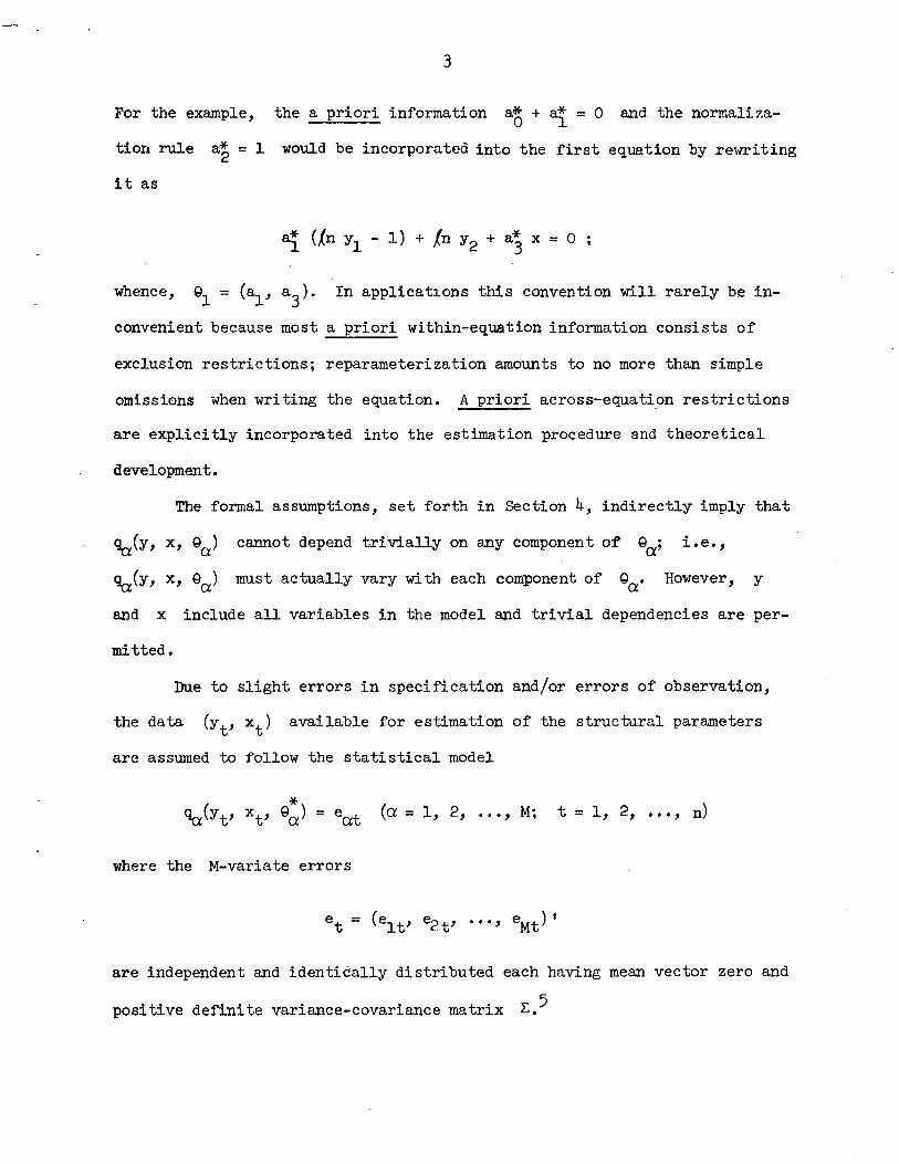
the a priori information a* + a* = 0 and the normali za­o 1

tion rule a2 = 1 would be incorporated into the first equation by rewriting

it as

whence, 91 = (al , a3

). In applicatlons this convention will rarely be in­

convenient because most a priori within-equation information consists of

exclusion restrictions; reparameterization amounts to no more than simple

omissi0ns when writing the equation. A priori across-equation restrictions

are explicitly incorporated into the estimation procedure and theoretical

development.

The formal assumptions, set forth in Section 4, indirectly imply that

~(y, x, 90) cannot depend trivially on any component of 90;; i. e.,

%:(y, x, 90;) must actually vary wi"th each component of Qo;o However, y

and x include all variables in the model and trivial dependencies are per-

mi tted.

Due to slight errors in specification and/or errors of observation,

the data (Yt' xt ) available for estimation of the structural parameters

are assumed to follow the statistical model

*~(Yt' xt ' 90;) = eo;t (0; = 1, 2, •• 0' M; t = 1, 2, ••• , n)

where the M-variate errors

are independent and identically distributed each having mean vector zero and

positive definite variance-covariance matrix ~.5

-'. 4

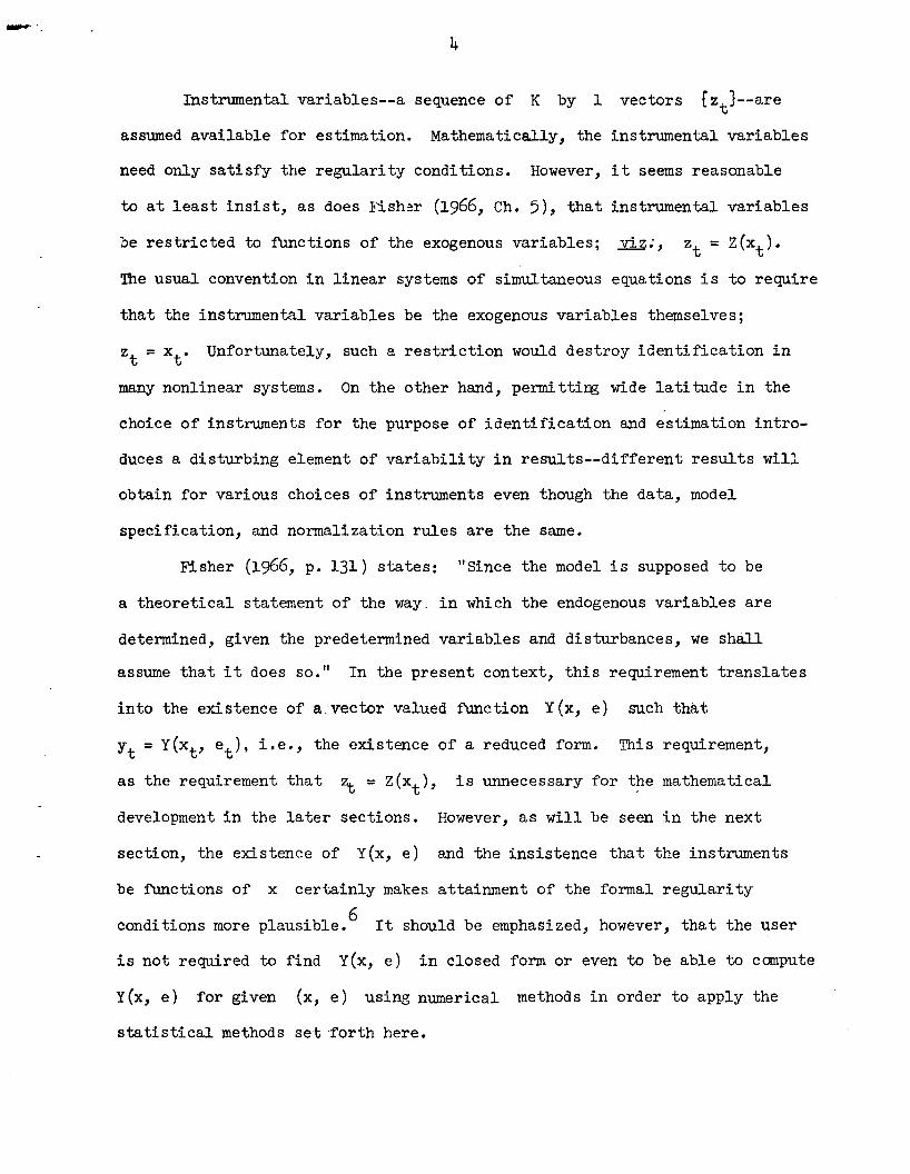
Instrumental variables--a sequence of K by 1 vectors fz }--aret

assumed available for estimation. Mathematically, the instrumental variables

need only satisfy the regularity conditions. However, it seems reasonable

to at least insist, as does Fish:r (1966, Ch. 5), that instrumental variables

oe restricted to functions of the exogenous variables; viz;, Zt = Z(xt ).

The usual convention in linear systems of simultaneous equations is to require

that the instrumental variables be the exogenous variables themselves;

Zt = xt • Unfortunately, such a restriction would destroy identification in

many nonlinear systems. On the other hand, permi ttir.g wide latitude in the

choice of instruments for the purpose of identification and estimation intro-

duces a disturbing element of variability in results--different results will

obtain for various choices of instruments even though the data, model

specification, and normalization rules are the same.

Fisher (1966, p. 131) states: "Since the model is supposed to be

a theoretical statement of the way_ in which the endogenous variables are

determined, given the predetermined variables and disturbances, we shall

assume that it does so." In the present context, this requirement translates

into the existence of a 'vector valued function Y(x, e) such that

Yt = Y(xt , et ), i.e., the existence of a reduced form. This requirement,

as the requirement that ~ = Z(xt ), is unnecessary for the mathematical

development in the later sections. However, as will be seen in the next

section, the existence of Y(x, e) and the insistence that the instruments

be functions of x certainly makes attainment of the formal regularity

conditions more Plausible. 6 It should be emphasized, however, that the user

is not required to find Y(x, e) in closed form or even to be able to compute

Y(x, e) for given (x, e) using numerical methods in order to apply the

statistical methods set forth here.

5

One detail should be mentioned before describing ~he estimation

procedure. The sequence of exogenous variables [xt } is assumed to be

either a sequence of constants or, if some coordinates are random variables,

the assumptions and results are conditional probability statements given the

sequence [Xt}--lagged endogenous variables are not permitted. Nevertheless,

the proofs, in fact, only require the stated regularity conditions with the

assumptions on the error process ret} modified to read: The conclusions

of Lemma A.3 are satisfied. Be that as it may, there are no results avail-

able in the probability literature, to the author's knowledge, which yield

the conclusions of Lemma A.3 for lagged endogenous instrumental variables

generated by a system of simultaneous, nonlinear, implicit equations. (The

requisite theory for the linear case is spelled out in Section 10.1 of

Theil (1971).) The reader who feels that these modified assumptions are

reasonable, in the absence of such results, may include lagged endogenous

variables as components of xt •

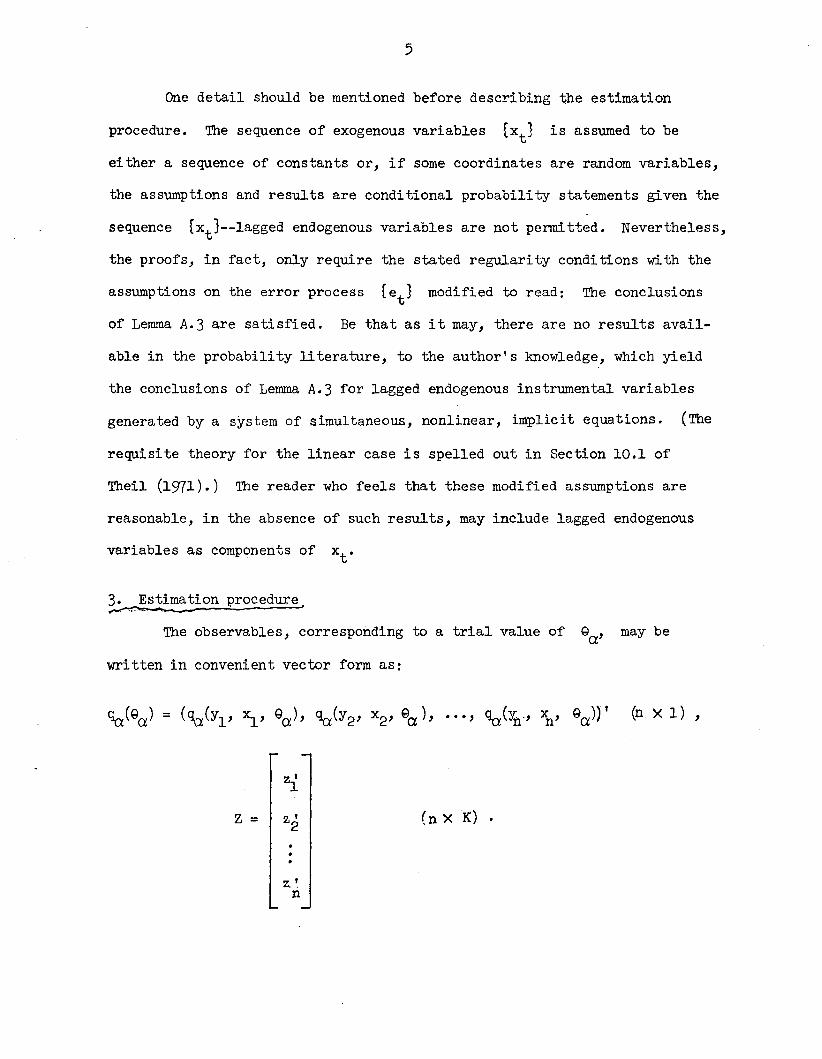
3. Estimation procedure.~. ~

The observables, corresponding to a trial value of Qa' may be

written in convenient vector form as:

z'1

x ,n (n X 1) ,

z = 2. '2

z'n

(n X K) •

6

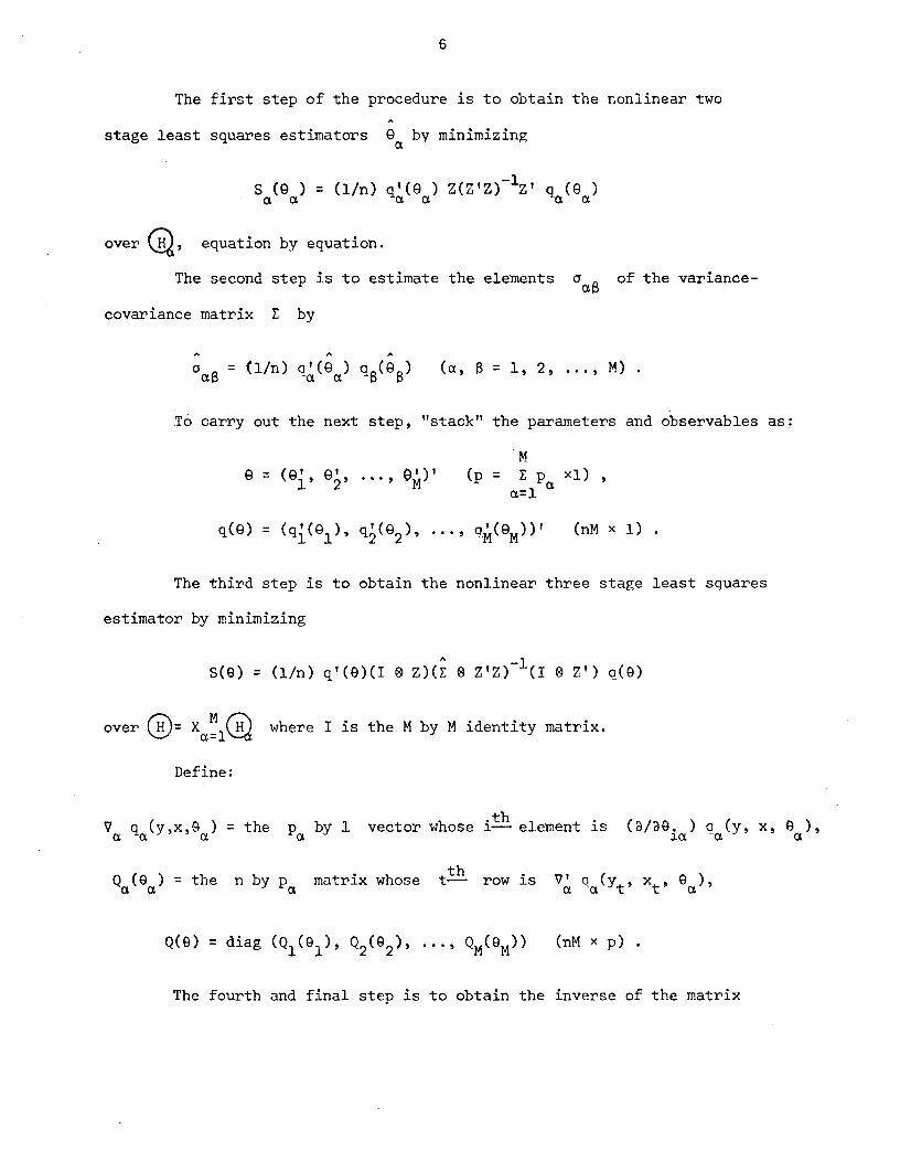
The first step of the procedure is to obtain the nonlinear two

stage least squares estimators e by minimizinga

s (e ) = (lIn) q'{e ) Z{ZIZ)-lZ' qa{ea

)a a a a

over~, equation by equation.

The second step is to estimate the elements

covariance matrix L by

of the variance-

A ...

°as = (lIn) q~{ea) QS{eS) (a, 13 = 1,2, ••• , M) •

.To carry out the next step, "stack" the parameters and observables as:

... , () I) IM

(p =ML p xl) ,

0.=1 a

(nM xl) •

The third step is to obtain the nonlinear three stage least squares

estimator by minimizing

over (E)= Xa~l~ where I is the Mby M identity matrix.

Define:

( ~) h b 1 h .th 1 .V q y,x,o = t e p y vector w ose l-- e ement lSa a a a(a/aG. ) a (y, x, e ),

la'a a

the n by pa

matrix whose tht-- row is

(nM x p) •

The fourth and final step is to obtain the inverse of the matrix

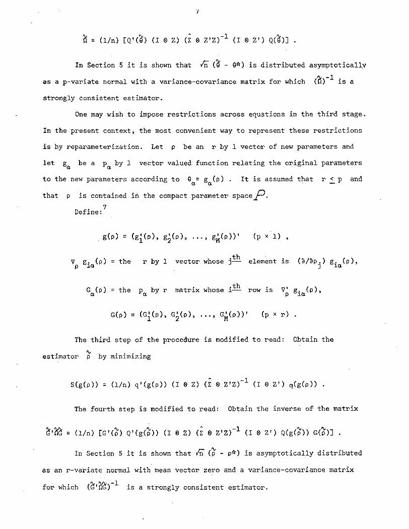
'?l = (lin) [Q'(~) (I ~ Z) 0: ~ 2 ' Z)-1 (I ~ 2 ' ) Q{~)] •

In Section 5 it is shown that In (~ - e*) is distributed asymptotically

as a p-variate normal with a variance-covariance matrix for which ('?l)-l is a

strongly consistent estimator.

One may wish to impose restrictions across equations in the third stage.

In the present context, the most convenient way to represent these restrictions

is by reparameterization. Let p be an r by 1 vector of new parameters and

let be a p by 1a

vector valued function relating the original parameters

to the new parameters according to e = g (p). It is assumed that r ~ p anda a

that p is contained in the compact parameter space~.

. 7DefJ.ne:

(p x 1) ,

gia(P) the r by 1 vector whose .th element is O/aP.) g. (p),V = J-p J J.a .

G (p) the p by r matrix whose .th is V' gia(P),= ].- rowa a P

G(p) = (Gi(p), G2(p), ... " GM(p)) 1 (p x r)

The third step of the procedure is modified to read: Obtain the

'"estimator p by minimizing

S(g{p)) = (lin) q'(g(p)) (I 0 Z) (r ~ ZIZ)-l (I ~ Z') q{g(p)) .

The fourth step is modified to read: Obtain the inverse of the matrix

In Section 5 it is shown that In (~ - p*) is asymptotically distributed

as an r-variate normal with mean vector zero and a variance-covariance matrix

for which (~,~)-l is a strongly consistent estimator.

8

If desired, results obtained subject to the restrictions Q = g(p)

may be reported in terms of the original parameters: Put Q= g(p). The

estimator Q is strongly consistent for *Q *and _yn (Q - Q ) is asympto-

..

tually distributed as a p-variate normal with mean vector zero and a variance

covariance matrix for which G(p) (G'nG)-l G' (p) is a strongly consistent

estimator. This matrix will be singular when r < p.

The computations may be performed using either Hartley's modified

Gauss-Newton method or Marquardt's algorithm. A program using one of these

algorithms is the preferred choice for the computations because they: are

widely available, perform well without requiring the user to supply second

partial derivatives, and will print the asymptotic variance-covariance

matrix needed to obtain standard errors. Our discussion of how they are

to be used depends on the notation in Section 1 of Gallant (1975b) and the

description of these algorithms in Section 3 of the same reference; the

reader will probably need this reference in hand to read the next few

paragraphs.

To use the algorithms as they are usually implemented, factor the

MK by MK matrix (i ® Z'Z)-l to obtain R such that R'R = (i ® Z'Z)-l;

then use the algorithms with these substitutions: y = 0, f(Q) = R(I ® Z') q(Q),

and F(Q) = R(I ® Z') Q(Q). Most implementations of these' algorithms expect

the user to supply a PL/l or FORTRAN subroutine to compute a row of f(Q)

or F(Q) given Q and the row index. (To be given an input vector xt

of f(Xt

, Q) is equivalent to having been given the row index.) This is

needlessly costly, for the present purpose, because it requires recomputation

of q(Q) and Q(Q) for every row. The difficulty can be circumvented since,

for each trial value of Q, the subroutine is always called sequentially with

9

the row index running from I = 1, 2, ••• , nM. The user-supplied subrou~ine

can be written so as to compute and store f(g) and F(g) when I = 1 and

then supply entries from these arrays for the subsequent calls: I = 2, ..., nM•

,. A (~) -1.,The matrix C printed by the program will satisfy nC =~, that is,,.

the diagonal entries of C...

are the estimated variances of g, whereas the

diagonal entries of (~)-l .r:: ...H are the estimated variances of Vn g. The

is, in this instance, a strongly consistent estimator of one.

standard errors for

the diagonal entries of2

s

printed by the program will have been computed from

s2 C and may be used after division by P;A good

choice for the starting value is go = 9 = (9i, Q~, .0., 9~)'.

Similarly, one may use these algorithms to compute P by putting

y = 0, f(p) = R(I 0 Z') q(g(p)), and F(p) = R(I 0 Z') Q(g(p)) G(p); the

matrix C will satisfy (G'OG)-l = nCo To compute the nonlinear two stage

least squares estimators Qa' factor the K by K matrix (z'Z)-l to

obtain R such that R'R = (Z'Z)-l then put y = 0, f(g) = R Z' ~(ga)'

and F(g) = R Z' ~ (ga).

4. Exogenous variables, assumptions, and identif~ation

The assumptions, given later in this section, used to obtain the

asymptotic theory of the nonlinear three stage least squares estimator,n .

require that sample moments such as (lin) L Zt ~(Yt' xt ' ga) converget=l

almost surely uniformly in gao It is obligatory, therefore, to set forth

reasonable conditions on the exogenous variables so that such limiting

behavior is achieved in applications. To illustrate one of the problems

involved, assume that the errors

10

are normally distributed. This implies that the function ~(y, x, Qa)

cannot be bounded, which effectively rules out the use of weak con-

vergence of measures as a means of imposing conditions on the sequence

of exogenous variables {xt } (Ma1invaud, 1970). We are led, therefore,

to define a similar but stronger notion.

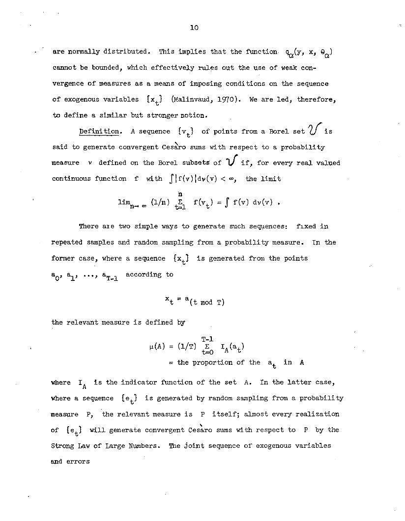
Defini tion. A sequence {vt} of points from a Borel set if is

said to

measure

generate convergent Ces~ro sums with respect to

v defined on the Borel subsets- of V if, for

a probability

every real valued

continuous function f with Slf(v) Idv(v) < CI:J, the limit

nlimn~ CI:J (lin) t~l f(vt ) = Sf(v) dv(v) •

There are two simple ways to generate such sequences: fl.xed in

repeated samples and random sampling from a probability measure. In the

former case, where a sequence {xt

} is generated from the points

aO' aI' ••• , aT_l according to

the relevant measure is defined by

T-l~(A) = (liT) t~o IA(at )

= the proportion of the at in A

where IA

is the indicator function of the set A. In the latter case,

where a sequence ret} is generated by random sampling from a probability

measure P, the relevant measure is P itself; almost every realization\

will generate convergent Cesaro sums with respect to P by the

Strong Law of Large Numbers. The joint sequence of exogenous variables

and errors

11

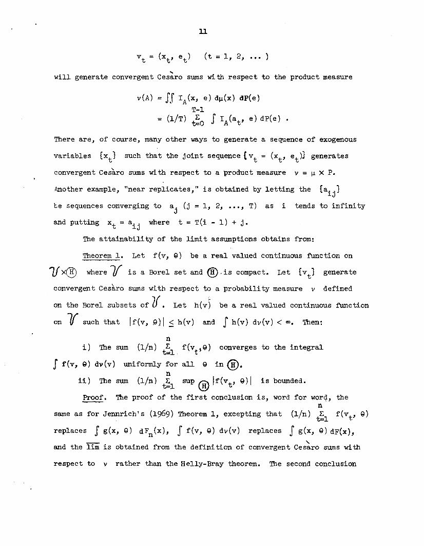
(t = 1, 2, ••• )

"-will generate convergent Cesaro sums with respect to the product measure

YeA) = IS IA(X, e) d~(x) dP(e)

T-l= (liT) ~o I IA(at , e) dP(e) •

There are, of course, many other ways to generate a sequence of exogenous

variables [xt } such that the joint sequence (vt = (xt

, e t ») generates

....convergent Cesaro sums with respect to a product measure v = ~ X P.

Another example, "near replicates," is obtained by letting the [aij }

te sequences converging to a. (j = 1, 2, ••• , T) as i tends to infinityJ

and putting xt = aij where t = T(i - 1) + j.

The attainability of the limit assumptions obtains from:

Theorem 1. Let f(v, Q) be a real valued continuous function on

1/X® where 7f is a Borel set and ®' is compact. Let [vt} generat.e

convergent Ces~ro sums with respect to

on the Borel subsets of 2(. Let h(v)

on {( such that If (v, g) I ::: h (v) and

a probability measure v defined

be a real valued continuous function

Sh(v) dv(v) <~. Then:

ni) 'lbe sum (lin) E f(V

t, Q) converges to the integral

t:::l

I f(v, Q) dv(v) uniformly for all Q in @.n

ii) The sum (lin) ~l sup ®'f(Vt , Q)I is bounded.

Proof. ~!e proof of the first conclusion is, word for wor9, then

same as for Jennrich's (1969) Theorem 1, excepting that (lin) ~l f(vt

, Q)

replaces Sg(x, Q) dFn(X), I f(v, Q) dv(v) replaces Sg(x, Q) dF(x),

"and the lim is obtained from the definition of convergent Cesaro sums with

respect to v rather than the Helly-Bray theorem. The second conclusion

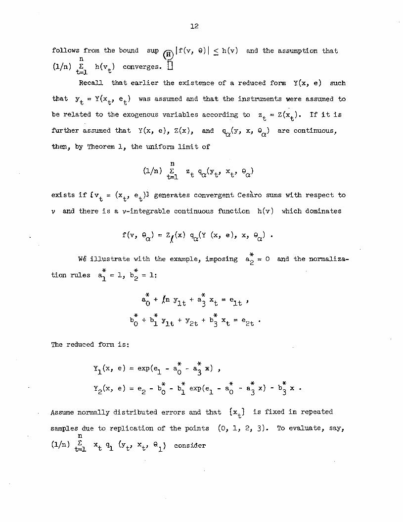
12

followsnfrom the bound sup ® If (v, Q) I ~ h (v) and the assumption that

(lin) t~l h(Vt ) converges. 0Recall that earlier the existence of a reduced form Y(x, e) such

that Yt = Y(xt , et ) was assumed and that the instruments were assumed to

be related to the exogenous variables according to Zt = Z(xt ). If it is

further assumed that Y(x, e), Z(x), and ~(y, x, Qa ) are continuous,

then, by Theorem 1, the uniform limit of

n(lin) ~l Zt ~(Yt' xt ' Qa )

exists if (vt = (xt , et )) generates convergent Cesaro sums with respect to

v and there is a v-integrable continuous fUnction h(v) which dominates

we illustrate with the example, imposing

* *tion rules al = 1, b2 = 1:

*a2

= 0 and the normaliza-

The reduced form is:

Yl(x, e)

Assume normally distributed errors and that {xt } is fixed in repeated

samples due to replication of the points (0, 1, 2, 3). To evaluate, say,n

(lin) t~l xt ql (Yt' xt ' Hl ) consider

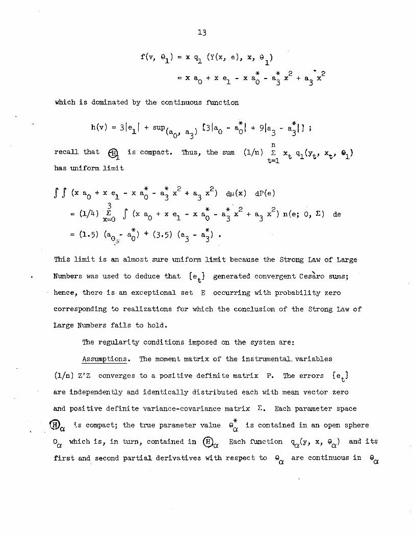
13

f(v, ~\) = x ql (Y(x, e), x, 91

)

* . * 2 • 2= x aO + x el - x aO - a3

x + a3

x

which is dominated by the continuous function

recall that ~ is compact.

has uniform limit

nThus, the sum (lin) E xt ql(Yt' xt ' ell

t=l

ss (x ao + x el - * * 2 2dJ..t(x) dP(e)x a - a

3x + a

3x )0

3S (x * * 2 2

= (1/4 ) . E aO + x el - x aO a3

x + a3

x ) n(e; 0, E) dex=O

(1. 5) * + (3.5) (a3

- *= (aO_- aO) a3

) •,;~

This limit is an almost sure uniform limit because the strong Law of Large

Numbers was used to deduce that ret},

generated convergent Cesaro sums;

hence, there is an exceptional set E occurring with probability zero

corresponding to realizations for which the conclusion of the strong Law of

Large Numbers fails to hold.

The regularity conditions imposed on the system are:

Assumptions. The moment matrix of the instrumental. variables

(lin) Z'Z converges to a positive definite matrix P. The errors ret}

are independently and identically distributed each with mean vector zero

and positive definite variance-covariance matrix E. Each parameter space

®a i.s compact; the true parameter value G~ is contained in an open sphere

0a which is, in turn, contained in ®a Each function ~(y, x, Ga ) and its

first and second partial derivatives with respect to Ga are continuous in Ga

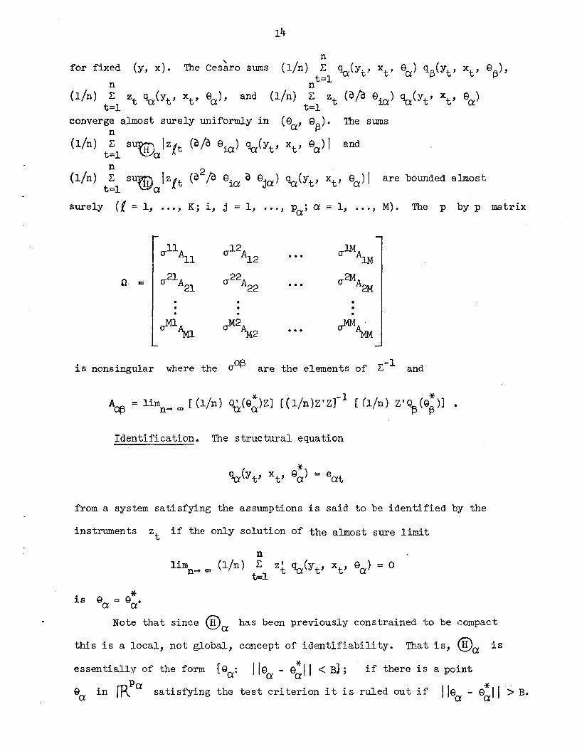
nfor fixed (y, x). The Ces~ro sums (lin) t:l ~(Yt' xt ' ea ) q(3(Yt' xt ' e(3)'

n n(lin) ~ Zt ~(Yt' xt ' ea ), and (lin) ~ Zt (0/0 em) ~(Yt' X t ' ea )

t=l t=lconverge almost surely uniformly in (e, e(3). The sums

n a

(lin) t:l SU®q IZit (0/0 eia) ~(Yt' x t ' ea ) I and

n 2(lin) L: SU~ 1ZIt (0 /0 eia 0 e

J·a ) '\:x(Yt' x t ' ea )I are bounded almost

t=l \!Y'a 1..

surely (i = 1, ---, K; i, j = 1, .--, Pa ; a = 1, , M). The p by p matrix

(fllA (f12A (f1MA11 12 1M

n = (f21A (f22A (f2MA21 22 2M

~\u ~2~2 ~.... ~

is nonsingular where the 0f3 -1(f are the elements of ~ and

Identification. The structural equation

from a system satisfying the assumptions is said to be identified by the

instruments Zt if the only solution of the almost sure limit

nlimn'" (Xl (lin) ~ zt, '\:x(Yt ' xt ' ea ) = 0

t=l

*is ea = ea·

Note that since ®a has been previously constrained to be eompact

this is a local, not global, concept of identifiability. That is, ~a is

essentially of the form tea: I lea - e~1 1< BJ; if there is a point

ea in rRPasatisfying the test criterion it is ruled out if Ilea - e~ll> B.

15

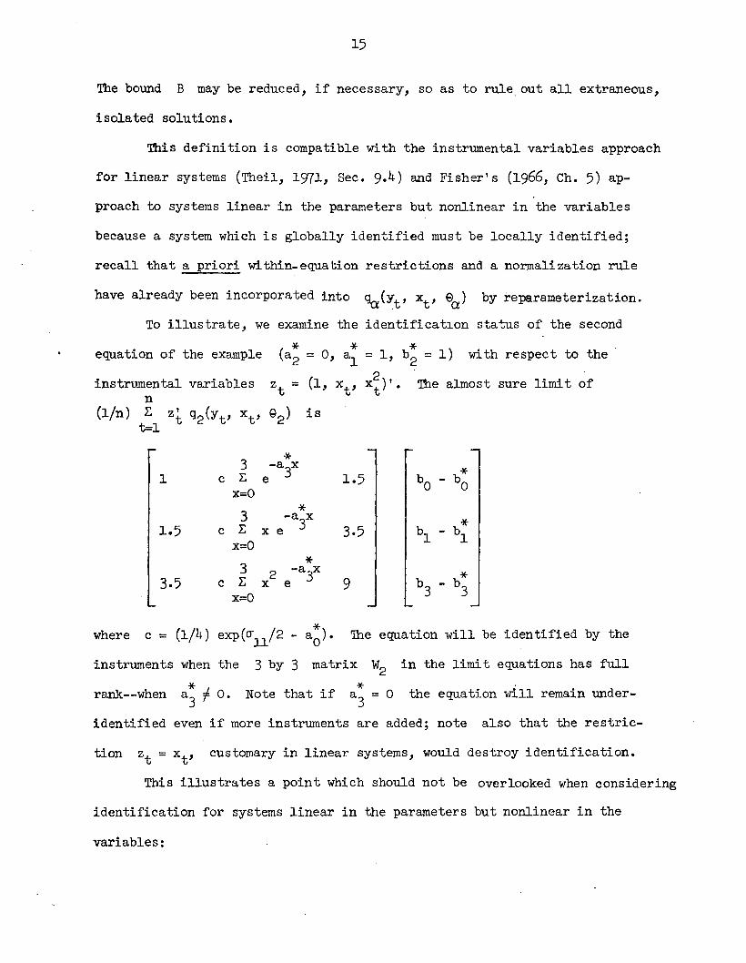
The bound B may be reduced, if necessary, so as to rule out all extraneous,

isolated solutions.

This definition is compatible with the instrumental variables approach

for linear systems (Theil, 1971, Sec. 9.4) and Fisher's (1966, Ch. 5) ap-

proach to systems linear in the parameters but nonlinear in the variables

because a system which is globally identified must be locally identified;

recall that a priori within-equation restrictions and a normalization rule

have already been incorporated into ~(Yt' xt ' ea ) by reparameterization.

To illustrate, we examine the identificatlon status of the second

equation of the example

instrumental variablesn

(l/n) ~ Zt Q2(Yt' xt 't=l

* *(a2 = 0, al

Zt = (1, xt '

Q2) is

*= 1, b2 = 1) with respect to the

x~) '. The almost sure limit of

1

1.5

3.5

3 *-a xc ~ e 3

x=o

*3 -a xc ~ x e 3

x=o

*3 2 -a xc ~ x e 3

x=o

1.5

3.5

9

*where c = (1/4) eXP(~11/2 - ao ). The equation will be identified by the

instruments when the 3 by 3 matrix W2 in the limit equations has full

rank--when Note that if the equation will remain under-

identified even if more instruments are added; note also that the restric-

tion Zt = xt ' customary in linear systems, would destroy identification.

This illustrates a point which should not be overlooked when considering

identification for systems linear in the parameters but nonlinear in the

variables:

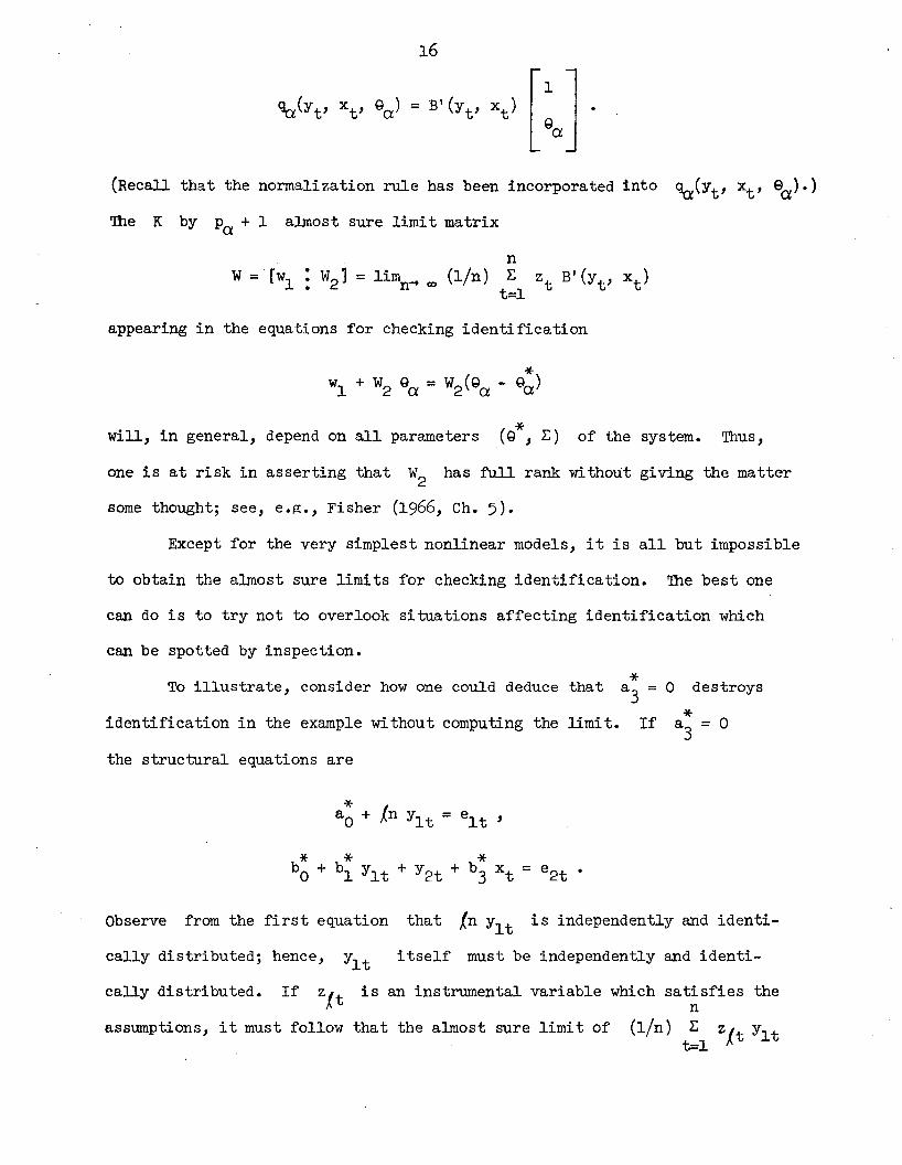
16

'!a(Yt , xt ' Gal = B' (Yt , xt ) [:a] ·

(Recall that the normalization rule has been incorporated into ~(Yt' xt ' ea ).)

The K by Pa + 1 almost sure limit matrix

nW=[wl : W2 ] = lim ~ (lin) E Zt B'(Yt , xt )

• n 00 t=l

appearing in the equations for checking identification

will, in general, depend on all parameters *(9 , E) of the system. Thus,

one is at risk in asserting that W2

has full rank without giving the matter

some thought; see, e.g., Fisher (1966, Ch. 5).

Except for the very simplest nonlinear models, it is all but impossible

to obtain the almost sure limits for checking identification. The best one

can do is to try not to overlook situations affecting identification which

can be spotted by inspection.

identification in the example without computing the limit.

To illustrate, consider how one could deduce that

the structural equations are

*a3

= 0 destroys

*If a3

= 0

Observe from the first equation that In Ylt is independently and identi-

cally distributed; hence, Ylt itself must be independently and identi-

assumptions, it must follow that the almost sure limit of

cally distributed. If is an instrumental variable which satisfies then

(lin) E ZIt Yltt=l "

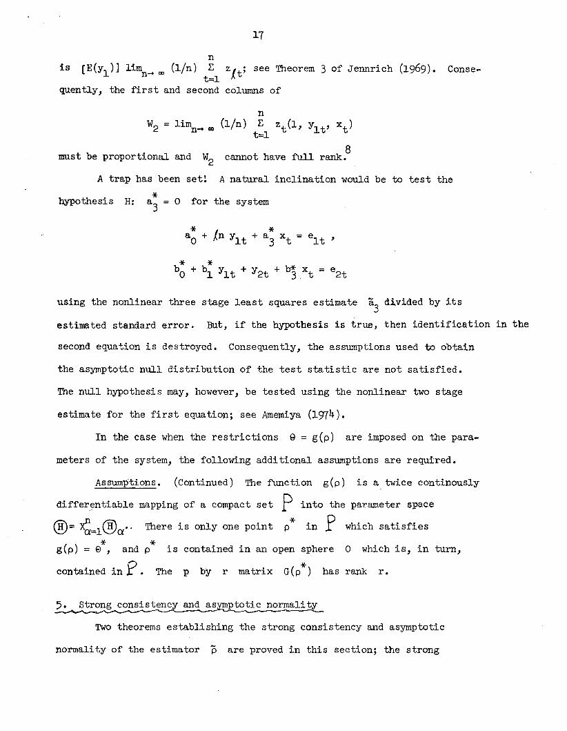
17

nis [E(Yl)] limn~ 00 (lin) ~ Z't; see Theorem 3 of Jennrich (1969). Conse­

t=l I-quently, the first and second columns of

W2 = limn~ co

must be proportionaJ. and W2

A trap has been setl

n(lin) ~ Zt(l, Ylt' x t )

t=l

8cannot have full rank.

A natural inclination would be to test the

hypothesis H: *a3

= a for the system

using the nonlinear three stage least squares estimate a3

divided by its

estimated standard error. But, if the hypothesis is true, then identification in the

second equation is destroyed. Consequently, the assumptions used to obtain

the asymptotic null distribution of the test statistic are not satisfied.

The null hypothesis may, however, be tested using the nonlinear two stage

estimate for the first equation; see Amemiya (1974).

In the case when the restrictions g = g(p) are imposed on the para-

meters of the system, the following additional assumptions are required.

Assumptions. (Continued) The fUnction g(p) is a twice continously

differentiable mapping of a compact set P into the parameter space

is contained in an open sphere

@= ~=l®a·· There is only one point

* *g(p) = e, and p

*p in P which satisfies

a which is, in turn,

contained in.P • The p hy r matrix *G(p ) has rank r.

5. strong consistency and as ptotic normality

Two theorems establishing the strong consistency and asymptotic

normality of the estimator p are proved in this section; the strong

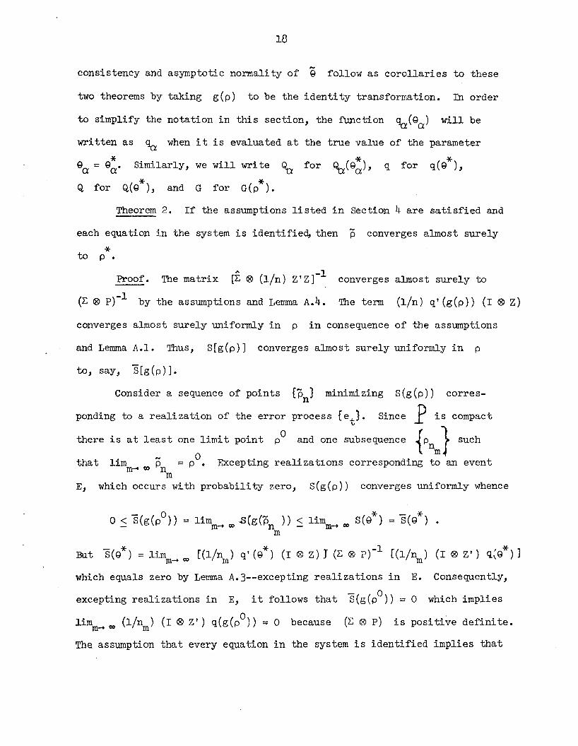
18

-consistency and asymptotic normality of Q follow as corollaries to these

two theorems by taking g(p) to be the identity transformation. In order

to simplify the notation in this section, the function ~(Qa) will be

written as ~ when it is evaluated at the true value of the parameter

* *Qa = Qa. Similarly, we will write ~ for ~(Qa)'

Q for Q(Q*), and G for G(p*).

q for *q(Q ),

Theorem 2. If the assumptions listed in Section 4 are satisfied and

each equation in the system is identifie~ then p converges almost surely

*to p.

Proof. The matrix r~ @ (lin) Z'Z]-l converges almost surely to

(~@ p)-l by the assumptions and Lemma A.4. The term (lin) q'(g(p» (I @ Z)

converges almost surely uniformly in p in consequence of the assumptions

and Lemma A.l. Thus, S[g(p)] converges almost surely uniformly in p

to, say, 8[g(p)].

Consider a sequence of points {Pn} minimizing S(g(p» corres­

ponding to a realization of the error process {et }. Since'p is compact

there is at least one limit point pO and one subsequence {Pnm~ such

that lim p = pO. Excepting realizations corresponding to an eventm~ 0') n

mE, which occurs with probability zero, S(g(p» converges uniformly whence

- ° ( (* -( *° <_ S(g(p » = lim E(g p » < lim S Q ) = S Q )m~ ClO n - m'" co

m

But 8(Q*) = lim [(lin) q' (Q*) (I @ z) J (~ @ pfl [(lin) (I @ z,) q~Q*)]~ClO ill m

which equals zero by Lemma A.3--excepting realizations in E. Consequently,

excepting realizations in E, it follows that 8(g(pO» = ° which implies

lim (lin) (I @ Z') q(g(pO» = ° because (~@ p) is positive definite.m~ co m

The assumption that every equation in the system is identified implies that

19

g(pO) = g* which, by assumption, implies ° *p = p • Thus, excepting

~ealizations in E, {Pn} has only one limit point which is *p • IJCorollary. If the assumptions listed in Section 4 are satisfied

and each equation in the system is identified, then Q converges almost

*surely to g.

Theorem 3. If the assumptions listed in Section 4 are satisfied

. *and each equation in the system is identified, then ~ (p - p) converges

in distribution to an r-variate normal with mean vector zero and variance­

covariance matrix (G'nG)-l. The matrix

(G'nG) = (lin) G' (p) Q.' (g(p)) (I @ Z) (I: @ z'zrl (r @ Z') Q.(g(p)) G(p)

converges almost surely to G'nG.

Proof• Define p = p if P is in ° and *p = p if P is not.

in 0. Set 9 = g(p). Since A/ll (p - p) converges almost surely to zero

by Theorem 2, it will suffice to prove the theorem for .p •.

The first order Taylor's expansion of q(g) may be written as

q(g) = q + Q. G(p - p*) + H(p - p*) where H is the nM by r matrix

thH = (Hi, H2, ... , liM) t; the tr= row of the n by r submatrix Ha is

(1/2 ) (p - p*) ''V~ <la(yt' xt ' gaCP)) where p varies with t and p and

lies on the line segment joining P *to p. A typical element of

is a finite sum of products composed of the terms (Pi - p:), the first and

second partial derivatives of gia(P) evaluated atn

p = P, (lin) ~ Zit (o/og'a) <la(Yt' xt ' ga(p)), andt=l 1'- J

n 2(lin) t:l Z!t(o IdgiaogJa ) <la(Yt' xt ' ga{P))' As a direct consequence of

the almost sure bounds imposed on these latter terms by assumption and the

almost sure convergence of .p

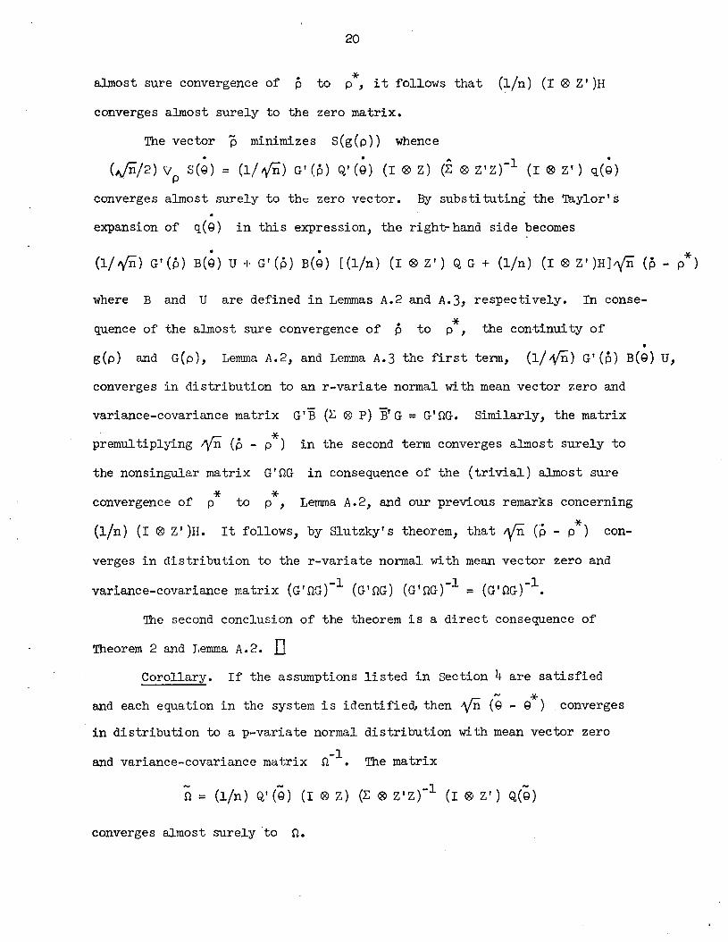
20

*to p, it follows that (l/n) (I ® Z')H

converges almost surely to the zero matrix.

The vector p minimizes S(g(p)) whence

(~/2) 'V s(~) = (1/ r(ii) G' (p) Q,' (~) (I ® Z) (£ ® z' zfl (I ® Z') q(~)p

converges almost surely to tht zero vector. By substituting the Taylor's

expansion of q(g) in this expression, the right-hand side becomes

.. *(l/,yn) G'(p) B(9) U+ G'(p) B(9) [(l/n) (I®Z') Q,G+ (l/n) (I®Z')H];y!ii (p - p)

where B and U are defined in Lemmas A.2 and A.3, respectively. In conse-

quence of the almost sure convergence of p to *p , the con-tinui ty of•

g(p) and G(p), Lemma A.2, and Lemma A.3 the first term, (1/1Ill) G'(p) B(9) U,

converges in distribution to an r-variate normal with mean vector zero and

variance-covariance matrix G'B (~ ® P) BIG = G'nG. Similarly, the matrix

premultiplying 1fO (p - p*) in the second term converges almost surely to

the nonsinglilar matrix G'nG in consequence of the (trivial) almost sure

* *convergence of p to p, Lemma A.2, and our previous remarks concerning

(l/n) (I ® z' )H. It follows, by Slutzky's theorem, that 1fn (p - p*) con-

verges in distribution to the r-variate normal with mean vector zero and

( -1 ( ( -1 ( -1variance-covariance matrix G'nG) G'nG) G'nG) = G'nG) •

The second conclusion of the theorem is a direct consequence of

Theorem 2 and Lemma A. 2. IJCorollary. If the assumptions listed in Section 4 are satisfied

,.. *and each equation in the system is identifie~ then ~ (g - g) converges

in distribution to a p-variate normal distribution with mean vector zero

d · . t· ~-lan varlance-covarlance ma rlX H • The matrix

n = (l/n) Q,' (9) (I ® Z) (~ ® z'zfl (I ® Z') Q,(g)

converges almost surely to n.

2l

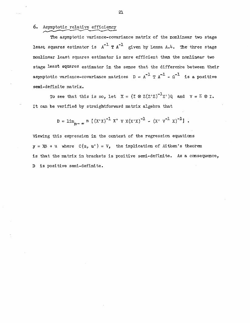
6. Asymptotic relative efficiency~--..-------

The asymptotic variance-covariance matrix of the nonlinear two stage

least squares estimator is A-I T A-I given by Lemma A.4. The" three stage

nonlinear least squares estimator is more efficient than the nonlinear two

stage least squares estimator in the sense that the difference between their

asymptotic variance-covariance matrices D = A-I T A-I - n-l is a positive

semi-definite matrix.

To see that this is so, let X = (I ® z(z'Z)-IZ')Q and V = ~ ® I.

It can be verified by straightforward matrix algebra that

Viewing this expression in the context of the regression equations

y =~ + u where C(u, u') = V, the implication of Aitken's theorem

is that the matrix in brackets is positive semi-definite. As a consequence,

D is positive semi-definite.

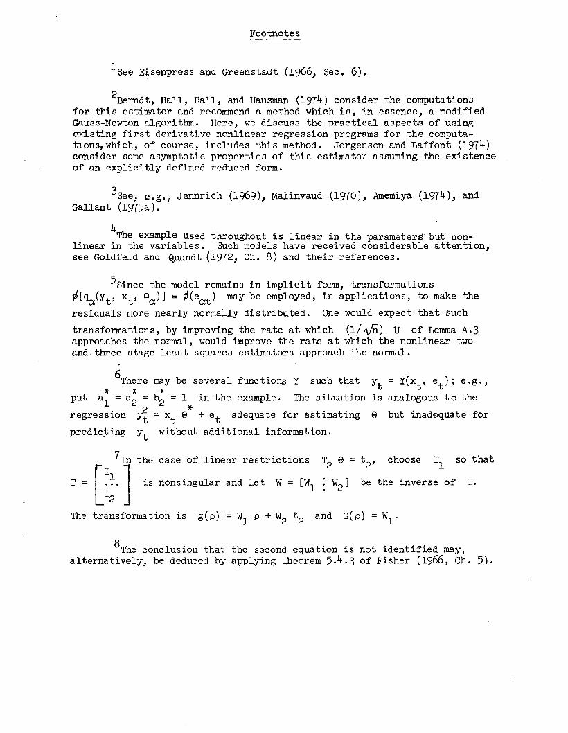
Footnotes

lSee Eisenpress and Greenstadt (1966, Sec. 6).

2Berndt, Hall, Hall, and Hausman (1974) consider the computationsfor this estimator and recommend a method which is, in essence, a modifiedGauss-Newton algorithm. Here, we discuss the practical aspects of usingexisting first derivative nonlinear regression programs for the computa­t10ns,which, of course, includes this method. Jorgenson and Laffont (1974)consider some asymptotic properties of this estimatoT assuming the existenceof an explicitly defined reduced form.

3see , e.g.; Jennrich (1969), Malinvaud (1970), Amemiya (1974), andGallant (1975a).

4The example Used throughout is linear in the parameters'but non-

linear in the variables. SUch models have received considerable attention,see Goldfeld and Quandt (1972, Ch. 8) and their references.

5Since the model remains in iwplicit form, transformations~[~(Yt' xt ' Qa)J = ~(eat) may be employed, in applications, to make the

residuals more nearly normally distributed. One would expect that such

transformations, by improving the rate at which (1/ '\fIi) U of Lemma A. 3approaches the normal, would improve the rate at which the nonlinear twoand three stage least squares estimators approach the normal.

6There may be several functions Y such that Yt = Y(xt , et ); e.g.,

* * *put a = a = b = 1 in the example. The situation is analogous to the1 2 2 *

regression ~ = xt e + e t adequate for estimating e but inadequate for

predic~ip~ Yt without additional information.

71n the case of linear restrictions T2 e = t 2, choose Tl so that

T = [:~. J iE nons ingular and 1e t W = [W1 : W2 J be the inverse of T.

The transformation is g(p) = WI P + W2 t 2 and G(p) = WI·

8The conclusion that the second equation is not identified may,alternatively, be deduced by applying 'Iheorem 5.4.3 of Fisher (1966 , Ch. 5).

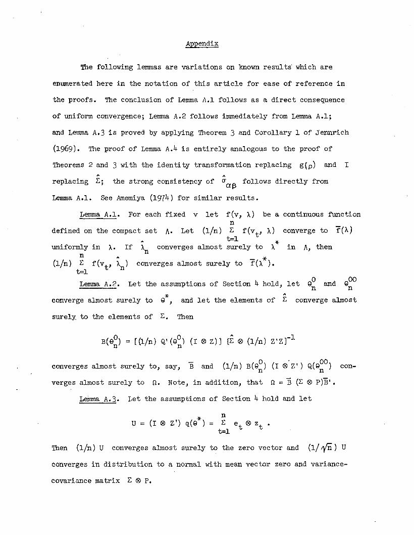
Appendix

The following lemmas are variations on known results' which are

enumerated here in the notation of this article for ease of reference in

the proofs. The conclusion of Lemma A.l follows as a direct consequence

of uniform convergence; Lemma A.2 follows immediately from Lemma A.l;

and Lemma A.3 is proved by applying Theorem 3 and Corollary 1 of Jennrich

(1969). The proof of Lemma A.4 is entirely analogous to the proof of

Theorems 2 and 3 with the identity transformation replacing g(p) and I~ ~

replacing ~; the strong consistency of crQ;f3 follows directly from

Lemma A.I. See Amemiya (1974) for similar results.

Let the assumptions of Section 4 hold, let gO and gOOn nLemma A.2.

Lemma A.I. For each fixed v let f(v, A) be a continuous functionn

defined on the compact set A. Let (l/n) ~ f(vt , A) converge to rCA)t=l *

If An converges almost surely to A in A, then

- *converges almost surely to f(A).

uniformly in A.n ~

(l/n) ~ f(vt

, A )t=l n

converge almost surely to *g ,~

and let the elements of ~ converge almost

surely to the elements of ~. Then

converges almost surely to, say, Band

verges almost surely to n. Note, in addition, that

(I ®' Z') Q(gOO)n

n = 13 (~ ® p)13' •

con-

Lemma A.3. Let the assumptions of Section 4 hold and let

*U = (I ® Z') q(g )

Then (l/n) U converges almost surely to the zero vector and (1/ ;y'il) U

converges in distribution to a normal with mean vector zero and variance-

covariance matrix ~ ® P.

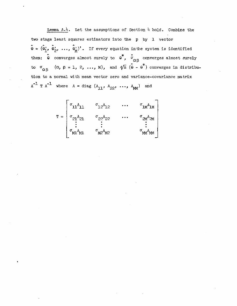
Lemma A.4. Let the assumptions of Section 4 hold. Combine the

two stage least squares estimators into the p by 1 vector...... ...

Q= (Qi, Q2' •.• , gM)'· If every equation inthe system is identified

then: Q

to 0"013

converges almost surely to

(0, 13 = 1, 2, ••• , M), and

*Q ,...0"013 converges almost surely

... *(Q - g ) converges in distribu-

tion to a normal with mean vector zero and variance-covariance matrix

-1 -1A T A where A = diag (All' A22, •••,~) and

O"llAll 0"1~12 ... O"~lM

T = 0"21A2l 0"22A22 ... 0"~2M

· • ·· · •• · ·O"Ml\U O"M2~2 O"MM~

References

Amemiya, T., 1974, "The nonlinear two-stage least-squares estimator," Journalof Econometrics 2, 105-110.

Berndt, E. K., B. H. Hall, R. E. Hall, and J. A. Hausman, 1974, fiEstimationand inference in nonlinear structural models," Annals of Economic andSocial Measurement 3, 653-666.

Eisenpress, H., and J. Greenstadt, 1966, "The estimation of nonlinear econo­metric systems," Econometrica 34, 851-861.

Fisher, F. M., 1966, The identification problem in econometrics (New York:McGraw-Hill) •

Gallant, A. R., 1975a, "Seemingly unrelated nonlinear regressions," Journalof Econometrics, 3, 35-50.

Gallant, A. R., 1975b, "Nonlinear regression," The American Statistician, 29,73-81.

Goldfeld, S. M., and R. E. Quandt, 1972, Nonlinear methods in econometrics(Amsterdam: North Holland).

Jennrich, R. 1., 1969, "Asymptotic properties of non-linear least squaresestimators," The Annals of MathematIcal Statistics 40, 633-643.

Jorgenson, D. W., and J. Laffont, 1974, "Efficient estimation of nonlinearsimultaneous equations with additive disturbances," Annals ofEconomic and Social Measurement 3, 615-640.

Malinvaud, E., 1970, "The consistency of nonlinear regressions," The Annalsof Mathematical Statistics 41, 956-969.

Theil, H., 1971, Principles of econometrics (New York: John Wiley and Sons).