Detection and Estimation Using Regularized Least Squares · Detection and Estimation Using...
90
Detection and Estimation Using Regularized Least Squares: Performance Analysis and Optimal Tuning Under Uncertainty Tareq Y. Al-Naffouri King Abdullah University of Science and Technology (KAUST) Communications Research Lab Ilmenau University of Technology Aug 9, 2018 1
Transcript of Detection and Estimation Using Regularized Least Squares · Detection and Estimation Using...

Detection and Estimation Using Regularized Least Squares:
Performance Analysis and Optimal Tuning Under Uncertainty
Tareq Y. Al-Naffouri
King Abdullah University of Science and Technology(KAUST)
Communications Research LabIlmenau University of Technology
Aug 9, 2018
1

Objective
y = Hx + z.
H is a linear transformation which might be uncertain (H + H )
H could be i.i.d random or ill-conditioned
z is the additive noise of unknown variance σ2z
x is the desired that we want to estimate or detect
x can be deterministic or random with unknown statistics
We will focus on regularized least-squares (and variants) fordetection/estimation
minx||y −Hx||2 + γ ||x||2
2

Optimal Tuning of Regularized Least Squares
Joint work with Mohamed Suliman & Tarig Ballal
3

Data model:y = Hx + z.
H ∈ Cm×n is the linear transformation matrix. (Known)
y ∈ Cm×1 is the observation vector. (Known)
x ∈ Cn×1 is the desired signal. (Unknown)
Stochastic: Rx , E(xxH
).
Deterministic: Rx , xxH .
4

Data model:y = Hx + z.
H ∈ Cm×n is the linear transformation matrix. (Known)
y ∈ Cm×1 is the observation vector. (Known)
x ∈ Cn×1 is the desired signal with covarince matrix Rx. (Unknown)
z ∈ Cm×1 is AWGN with variance σ2z. (Unknown)
z and x are independent.
Problems
Given y and H, find an estimate of x.
Optimally tune γ
4
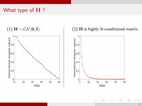
What type of H ?
(1) H ∼ CN (0, I).
Index0 10 20 30 40 50
Naro
maliz
ed s
ingula
r valu
es
0
0.2
0.4
0.6
0.8
1
(2) H is highly ill-conditioned matrix.
Index0 10 20 30 40 50
Norm
aliz
ed s
ingula
r valu
es
0
0.2
0.4
0.6
0.8
1
5

What type of H ?
(1) H ∼ CN (0, I).
Index0 10 20 30 40 50
Naro
maliz
ed s
ingula
r valu
es
0
0.2
0.4
0.6
0.8
1
Condition Number =1.821× 10³.
(2) H is highly ill-conditioned matrix.
Index0 10 20 30 40 50
Norm
aliz
ed s
ingula
r valu
es
0
0.2
0.4
0.6
0.8
1
30 40 50
×10-3
0
0.5
1
1.5
2
2.5
3
Condition Number = 2.49× 1028.
5
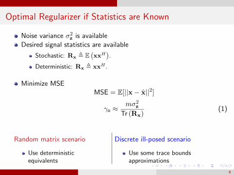
Optimal Regularizer if Statistics are Known
Noise variance σ2z is available
Desired signal statistics are available
Stochastic: Rx , E(xxH
).
Deterministic: Rx , xxH .
Minimize MSEMSE = E[||x− x||2]
γo ≈mσ2
z
Tr (Rx)(1)
Random matrix scenario
Use deterministicequivalents
Discrete ill-posed scenario
Use some trace boundsapproximations
6

Relation Between γo and the LMMSE
Our optimal regularizer is γo ≈ mσ2z
Tr(Rx) .
Note that the LMMSE is given by
xLMMSE =(HHH + σ2
zR−1x
)−1HHy. (2)
When x is i.i.d. with zero mean, Rx = σ2xI.
γo = σ2z
Tr(Rx)/m = σ2zσ2x.
This shows that γo is optimal when the input is white.
7

Proposed Approach
Recall the model: y = Hx + z.
Recall how the SV structure affects the result.
We propose adding perturbation ∆H ∈ Cm×n to H.
We will impose bound on ∆H (i.e., 0 ≤ ||∆H||2 ≤ λ ), why ?
Perturbed model:y ≈ (H + ∆H)x + z. (3)
Problem We know neither ∆H nor λ.
Judicious choice of λ is necessary.
8
Proposed Approach
We call the proposed approach COnstrained PerturbationRegularization Approach (COPRA).
9

COPRA
For now, let us assume we know the best choice of λ.
We propose bounding the worst-case residual error
minx
max∆H||y − (H + ∆H) x||2
subject to: ||∆H||2 ≤ λ. (4)
10

COPRA
For now, let us assume we know the best choice of λ.
We propose bounding the worst-case residual error
minx
max∆H||y − (H + ∆H) x||2
subject to: ||∆H||2 ≤ λ. (4)
After manipulations, the problem can be reduced to
minx
max∆H||y − (H + ∆H) x||2 = min
x||y −Hx||2 + λ ||x||2.
subject to: ||∆H||2 ≤ λ (5)
10
COPRA
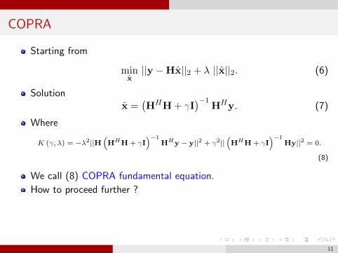
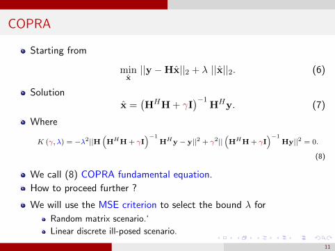
Starting from
minx||y −Hx||2 + λ ||x||2. (6)
Solutionx =
(HHH + γI
)−1HHy. (7)
Where
K (γ, λ) = −λ2||H(HHH + γI
)−1HHy − y||2 + γ2||
(HHH + γI
)−1Hy||2 = 0.
(8)
We call (8) COPRA fundamental equation.
How to proceed further ?
We will use the MSE criterion to select the bound λ for
Random matrix scenario.‘
Linear discrete ill-posed scenario.
11
COPRA
Starting from
minx||y −Hx||2 + λ ||x||2. (6)
Solutionx =
(HHH + γI
)−1HHy. (7)
Where
K (γ, λ) = −λ2||H(HHH + γI
)−1HHy − y||2 + γ2||
(HHH + γI
)−1Hy||2 = 0.
(8)
We call (8) COPRA fundamental equation.
How to proceed further ?
We will use the MSE criterion to select the bound λ for
Random matrix scenario.‘
Linear discrete ill-posed scenario.
11

(1) Random Matrix Scenario.
12

How to Find the Perturbation Bound λ ? (1) RandomScenario (R-COPRA)
Recall COPRA fundamental equation (8)
γo2||(HHH + γoI
)−1Hy||2 − λo
2||H(HHH + γoI
)−1HHy − y||2 = 0.
Consider obtaining a perturbation bound that is approximatelyfeasible for all the cases
λo2 E[σ2zTr
(HHH
(HHH +mγoI
)−2)
︸ ︷︷ ︸Q(γo)
+ Tr
((HHH +mγoI
)−2HHHRx
)︸ ︷︷ ︸
R(γo)
]
≈ E[σ2zTr
(HHH
(HHH +mγoI
)−2)
︸ ︷︷ ︸G(γo)
+ Tr
(HHH
(HHH +mγoI
)−2HHHRx
)︸ ︷︷ ︸
T (γo)
].
(9)
13

E (Q (γo)) =
σ2z
(√γo+4γo− 1)3(
1− 14
(√γo+4γo− 1)2γo
)γo
3
8
(γo
2 − 116
(√γo+4γo− 1)4γo
4
) +O(m−2
). (10)
E (R (γo)) =γo
(√γo+4γo− 1)3
Tr (Rx)
4m(
4− γo
(√γo+4γo− 1)) +O
(m−2
). (11)
E (T (γo)) =γo
4
(−1 +
√γo + 4
γo
)2
Tr (Rx)−γo
2(−1 +
√γo+4γo
)3Tr (Rx)
4(−4 + γo
(−1 +
√γo+4γo
)) +O(m−2
).
(12)
14

R-COPRA
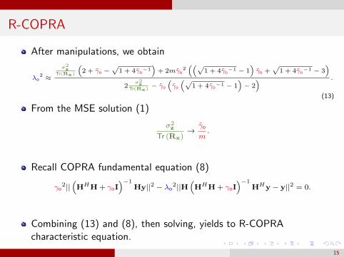
After manipulations, we obtain
λo2 ≈
σ2z
Tr(Rx)
(2 + γo −
√1 + 4γo
−1)+ 2mγo
2((√
1 + 4γo−1 − 1
)γo +
√1 + 4γo
−1 − 3)
2σ2z
Tr(Rx)− γo
(γo
(√1 + 4γo
−1 − 1)− 2) .
(13)
15
R-COPRA
After manipulations, we obtain
λo2 ≈
σ2z
Tr(Rx)
(2 + γo −
√1 + 4γo
−1)+ 2mγo
2((√
1 + 4γo−1 − 1
)γo +
√1 + 4γo
−1 − 3)
2σ2z
Tr(Rx)− γo
(γo
(√1 + 4γo
−1 − 1)− 2) .
(13)
From the MSE solution (1)
σ2z
Tr (Rx)→
γo
m.
Recall COPRA fundamental equation (8)
γo2||(HHH + γoI
)−1Hy||2 − λo
2||H(HHH + γoI
)−1HHy − y||2 = 0.
Combining (13) and (8), then solving, yields to R-COPRAcharacteristic equation.
15

R-COPRA
R-COPRA Characteristic Equation
SR (γo) = Tr(Σ2(Σ2 +mγoI
)−2bbH
)[γo
(√γo + 4
γo− 1
)− 4
]
+ Tr((
Σ2 +mγoI)−2
bbH)[
mγo
((√γo + 4
γo− 1
)γo + 2
√γo + 4
γo− 4
)]= 0, (14)
where b = UHy.
Solving SR (γo) results in the regularization parameter γo.
Question Can we solve (14) ?
16
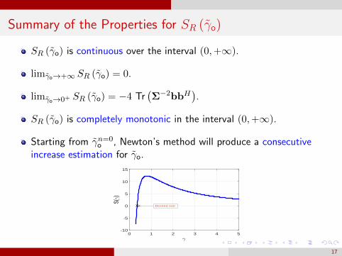
Summary of the Properties for SR (γo)
SR (γo) is continuous over the interval (0,+∞).
limγo→+∞ SR (γo) = 0.
limγo→0+ SR (γo) = −4 Tr(Σ−2bbH
).
SR (γo) is completely monotonic in the interval (0,+∞).
Starting from γn=0o , Newton’s method will produce a consecutive
increase estimation for γo.
γ
0 1 2 3 4 5
S(γ)
-10
-5
0
5
10
15
x Desired root
17

Simulation Results: Stochastic x
−10 0 10 20 30
−10
0
10
20
SNR [dB]
NM
SE
[dB
]
L-curveGCVQuasiR-COPRA
(a) x is i.i.d.
−10 0 10 20 30
−10
0
10
20
SNR [dB]N
MS
E[d
B]
L-curveGCVQuasiR-COPRA
(b) x is i.n.d.
Figure: NMSE versus SNR for H ∼ N (0, I),H ∈ R100×100.
18

Simulation Results: Deterministic x
−10 0 10 20 30
−10
0
10
20
SNR [dB]
NM
SE
[dB
]
L-curveGCVQuasiR-COPRA
Figure: NMSE versus SNR for H ∼ N (0, I),H ∈ R100×100 and x is square pulsesignal.
19

Simulation Results: Imperfect H
−10 0 10 20 30
10−3
10−2
10−1
100
Eb/No [dB]
BE
R LSL-curveQuasiGCVR-COPRA
(a) Perfect H.
−10 0 10 20 3010−3
10−2
10−1
100
Eb/No [dB]B
ER LS
L-curveQuasiGCVR-COPRA
(b) Imperfect H: H = H− eΩ.
Figure: BER comparison when H ∼ CN (0, I),H ∈ C100×100 and x is 8-QAMsignal.
20

Average Run Time
−10 0 10 20 300
1
2
3
4
5·10−2
SNR [dB]
Ave
rage
run
tim
e[s
ec]
L-curveQuasiGCVR-COPRA
Figure: Average run time.
21

(2) Ill-posed Scenario.
22
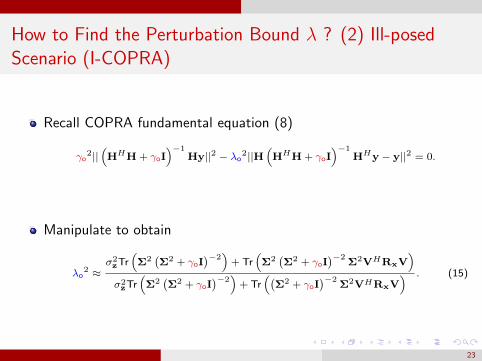
How to Find the Perturbation Bound λ ? (2) Ill-posedScenario (I-COPRA)
Recall COPRA fundamental equation (8)
γo2||(HHH + γoI
)−1Hy||2 − λo
2||H(HHH + γoI
)−1HHy − y||2 = 0.
Manipulate to obtain
λo2 ≈
σ2zTr
(Σ2(Σ2 + γoI
)−2)
+ Tr(Σ2(Σ2 + γoI
)−2Σ2VHRxV
)σ2zTr
(Σ2(Σ2 + γoI
)−2)
+ Tr((
Σ2 + γoI)−2
Σ2VHRxV) . (15)
23
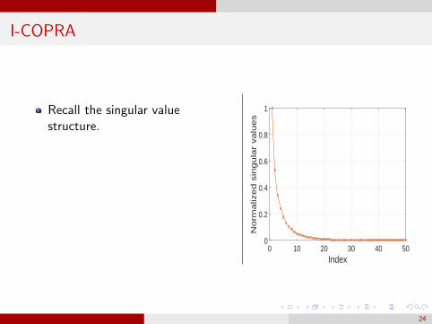
I-COPRA
Recall the singular valuestructure.
Index0 10 20 30 40 50
Norm
aliz
ed s
ingula
r valu
es
0
0.2
0.4
0.6
0.8
1
24
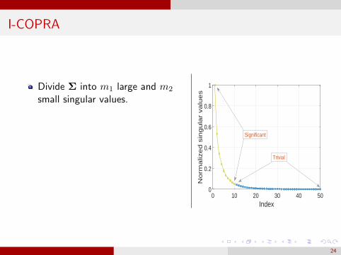
I-COPRA
Divide Σ into m1 large and m2
small singular values.
Index0 10 20 30 40 50
Norm
aliz
ed s
ingula
r valu
es
0
0.2
0.4
0.6
0.8
1
Trivial
Significant
24

I-COPRA
Divide Σ into m1 large and m2
small singular values.
Write Σ =
[Σ1 00 Σ2
]Σ1 ∈ Rm1×m1 (large singularvalues).
Σ2 ∈ Rm2×m2 (small singularvalues).
‖Σ2‖2 ‖Σ1‖2.Index
0 10 20 30 40 50N
orm
aliz
ed s
ingula
r valu
es
0
0.2
0.4
0.6
0.8
1
Trivial
Significant
24

Recall the optimal bound relation (15)
λo2 ≈
σ2zTr
(Σ2(Σ2 + γoI
)−2)
+ Tr(Σ2(Σ2 + γoI
)−2Σ2VHRxV
)σ2zTr
(Σ2(Σ2 + γoI
)−2)
+ Tr((
Σ2 + γoI)−2
Σ2VHRxV) .
Apply the partitioning to (15), with some manipulations andreasonable approximations to obtain
λo2 ≈
Tr
(Σ2
1
(Σ2
1 + γoI1
)−2(
Σ21 +
m1σ2z
Tr(Rx)I1
))Tr((
Σ21 + γoI1
)−2(Σ2
1 +m1σ2
zTr(Rx)
I1
))+ m2γo
2
m1σ2z
Tr(Rx)
. (16)
From the MSE solutionm1σ2
z
Tr (Rx)→
m1γo2
m.
From COPRA fundamental equation (8)
γo2||(HHH + γoI
)−1Hy||2 − λo
2||H(HHH + γoI
)−1HHy − y||2 = 0.
Combining (16) and (29), then solving, yields to I-COPRAcharacteristic equation.
25

I-COPRA
I-COPRA Characteristic Equation
SI (γo) = Tr(Σ2(Σ2 + γoI
)−2bbH
)Tr((
Σ21 + γoI1
)−2 (βΣ2
1 + γoI1
))+m2
γoTr(Σ2(Σ2 + γoI
)−2bbH
)− Tr
((Σ2 + γoI
)−2bbH
)× Tr
(Σ2
1
(Σ2
1 + γoI1
)−2 (βΣ2
1 + γoI1
))= 0, (17)
where b , UHy and β = mm1
.
Solving SI (γo) results in the regularization parameter γo.
The properties of the SI (γo) are studied and it is shown thatNewton’s method converges to the solution.
We studied the special case of this function when m1 = n andm2 = 0 in [2].
[2] T. Ballal, M. Suliman, T. Y. Al-Naffouri, and K. N. Salama, ”Constrained perturbation regularization algorithm for linear
least-squares problems”. Submitted to TSP, 2016.
26

I-COPRA Properties
γ
0 1 2 3 4 5
S(γ
)
-10
-5
0
5
10
15
x Desired root
27

Simulation Results. (2) I-COPRA
The algorithm is applied to a set of 11 real-worlds discrete ill-posedproblems.
28

Simulation Results. (2) I-COPRA
The algorithm is applied to a set of 11 real-worlds discrete ill-posedproblems.
28
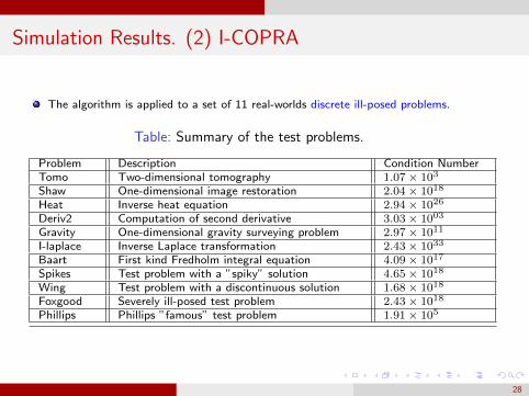
Simulation Results. (2) I-COPRA
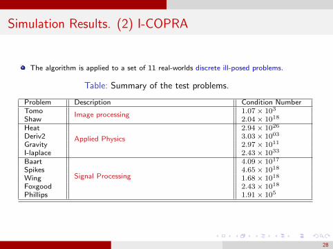
The algorithm is applied to a set of 11 real-worlds discrete ill-posed problems.
Table: Summary of the test problems.
Problem Description Condition NumberTomo Two-dimensional tomography 1.07× 10³
Shaw One-dimensional image restoration 2.04× 10¹⁸
Heat Inverse heat equation 2.94× 1026
Deriv2 Computation of second derivative 3.03× 1003
Gravity One-dimensional gravity surveying problem 2.97× 10¹¹
I-laplace Inverse Laplace transformation 2.43× 1033
Baart First kind Fredholm integral equation 4.09× 10¹⁷
Spikes Test problem with a ”spiky” solution 4.65× 10¹⁸
Wing Test problem with a discontinuous solution 1.68× 10¹⁸
Foxgood Severely ill-posed test problem 2.43× 10¹⁸
Phillips Phillips ”famous” test problem 1.91× 10⁵
28
Simulation Results. (2) I-COPRA
The algorithm is applied to a set of 11 real-worlds discrete ill-posed problems.
Table: Summary of the test problems.
Problem Description Condition NumberTomo Image processing 1.07× 10³
Shaw 2.04× 10¹⁸
Heat
Applied Physics
2.94× 1026
Deriv2 3.03× 1003
Gravity 2.97× 10¹¹
I-laplace 2.43× 1033
Baart
Signal Processing
4.09× 10¹⁷
Spikes 4.65× 10¹⁸
Wing 1.68× 10¹⁸
Foxgood 2.43× 10¹⁸
Phillips 1.91× 10⁵
28
Simulation Results. (2) I-COPRA
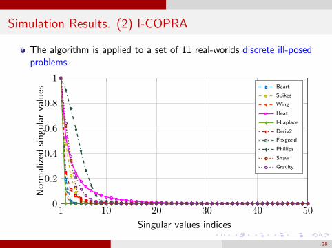
The algorithm is applied to a set of 11 real-worlds discrete ill-posedproblems.
1 10 20 30 40 500
0.2
0.4
0.6
0.8
1
Singular values indices
Nor
mal
ized
sin
gula
rva
lues
Baart
Spikes
Wing
Heat
I-Laplace
Deriv2
Foxgood
Phillips
Shaw
Gravity
28

Heat Problem
0 20 40 60 80 1000
0.2
0.4
0.6
0.8
1
Index
Nor
mal
ized
sin
gula
rva
lue
Singular values.
−10 0 10 20 30
0
20
40
60
SNR [dB]N
MS
E[d
B]
Proposed
Quasi
GCV
L-curve
Performance.
Condition number of H = 6.8× 1036. (m1 = 10,m2 = 40).
29

Baart Problem
0 20 40 60 80 1000
0.2
0.4
0.6
0.8
1
Index
Nor
mal
ized
sin
gula
rva
lue
Singular values.
−10 0 10 20 30−15
−10
−5
0
SNR [dB]N
MS
E[d
B]
Proposed
Quasi
L-curve
Performance.
Condition number of H = 2.89× 10¹⁸. (m1 = 3,m2 = 47).
30

Wing Problem
0 10 20 30 40 500
0.2
0.4
0.6
0.8
1
Index
Nor
mal
ized
sin
gula
rva
lue
Singular values.
−10 0 10 20 30
−4
−2
0
SNR [dB]N
MS
E[d
B]
L-curveQuasiI-COPRA
Performance.
Condition number of H = 1.68× 10¹⁸. (m1 = 3,m2 = 47).
31

Rank Deficient Matrices
−10 0 10 20 30
0
20
40
SNR [dB]
NM
SE
[dB
]
QuasiL-curveI-COPRA
(a) x is i.i.d.
−10 0 10 20 30
0
20
40
SNR [dB]
NM
SE
[dB
]
QuasiL-curveI-COPRA
(b) x is i.n.d.
Figure: H = 150BBH , where B ∼ N (0, I),B ∈ R50×45.
32

Special Case: (m1 = n and m2 = 0)
−10 0 10 20 30
−20
0
20
SNR [dB]
NM
SE
[dB
]
LSL-curveGCVQuasiI-COPRA
Figure: H ∈ R100×100 is Toeplitz matrix and x is i.i.d.
Condition number of H = 389.51.33

Example of the Average Run Time
−10 0 10 20 300
1
2
3
4
5·10−2
SNR [dB]
Ave
rage
run
tim
e[s
ec]
L-curveQuasiGCVI-COPRA
Figure: Average run time
34
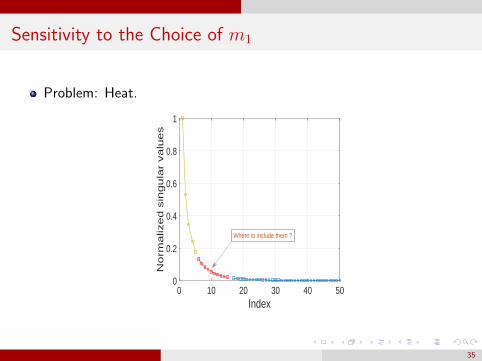
Sensitivity to the Choice of m1
Problem: Heat.
Index0 10 20 30 40 50
Norm
alized s
ingula
r valu
es
0
0.2
0.4
0.6
0.8
1
Where to include them ?
35
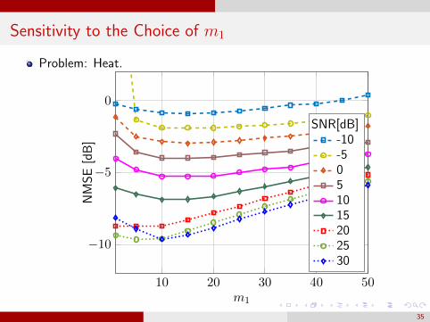
Sensitivity to the Choice of m1
Problem: Heat.
10 20 30 40 50
−10
−5
0
m1
NM
SE
[dB
]
SNR[dB]-10-5051015202530
35

Discriminant Analysis
Widely used statistical method for supervised classificationPrinciple: Builds a classification rule that allows to assign for anunseen observation its corresponding class.
Let x be the input data and f be the classification rule.
Classifier ,
Assign class 1 if f(x) => 0
Assign class 2 if f(x) =< 0
36

Gaussian Discriminant Analysis
Gaussian mixture model for binary classification (2 classes)
x1, · · · , xn ∈ Rp
Class k is formed by x ∼ N (µk,Σk), k = 0, 1
LDA Decision rule is linear in x:Σ0 = Σ1
WLDA = (x− µ0+µ1
2 )TΣ−1(µ0 − µ1)− π1π0
)Assign x to class 0 if WLDA > 0
Assignx to class 1 if otherwise
Statistics are unknown and so need to be estimated.
Covariance matrix will be ill-conditioned when sample size is less thanthe data dimension p.
Regularization could solve the problem but the choice of theregularization parameter is an issue.
37

Re-write the LDA score function as
WLDA(x) = (x− µ0 + µ1
2)T Σ−1(µ0 − µ1)
= aT Σ−1/2Σ−1/2b
= wT z
where
w = Σ−1/2a & z = Σ−1/2b
which can be obtained by solving the liner systems
a = Σ1/2w & b = Σ1/zb
38

Classification of digits from MINST data set
50 100 150 200 250 300
6
7
8
9
10
11
12
# of samples
MNIST (5,8)
50 100 150 200 250 3006
7
8
9
10
11
# of samples
Avg
. P
erc
en
tag
e E
rro
r
MNIST (7,9)
50 100 150 200 250 300
6
8
10
12
14
16
18MNIST (4,9)
50 100 150 200 250 3001.5
2
2.5
3
3.5
Avg
. P
erc
en
tag
e E
rro
r
MNIST (1,7)
RLDA (γ=1) GCV DAS RRLDA
Figure: Error rate performance of different LDA classifiers using handwrittendigits from MNIST dataset. The results are averaged over 50 Monte Carlo trials.
39

Beamforming
The output of the beamformer can be written as
yBF[t] = wHy[t], (18)
For the Capon/MVDR beamformer, the weighing coefficients aregiven by
wMVDR =C−1
yya
aHC−1yya
, (19)
where a is the array steering vector and Cyy is the sample covariancematrix of the received signals.Based on (18) and (19), we can write
yBF[t] =aHC
− 12
yy C− 1
2yy y
aH C− 1
2yy C
− 12
yy a=
bHz
bHb, (20)
where b , C− 1
2yy a and z , C
− 12
yy y.40

Application: Beamforming
The two relationships of a and b can be thought of as
a = C12yyb, (21)
and
y = C12yyz. (22)
Since C12yy is ill-conditioned, direct inversion does not provide a viable
solution.
Our regularization approach can be used to obtain estimates of b andz given that they are noisy.
41

Application: Beamforming
Recall (20)
yBF[t] =aHC
− 12
yy C− 1
2yy y
aH C− 1
2yy C
− 12
yy a=
bHz
bHb, (23)
Using regularization we can write
yBF-RLS =aHU
(Σ2 + γbI
)−1 (Σ2 + γzI
)−1Σ2UHy
aHU(Σ2 + γbI
)−2Σ2UHa
, (24)
Equation (24) suggests that the weighting coefficients for the RLSapproach are given by
wBF-RLS =aHU
(Σ2 + γbI
)−1 (Σ2 + γzI
)−1Σ2UH
aHU(Σ2 + γbI
)−2Σ2UHa
. (25)
42
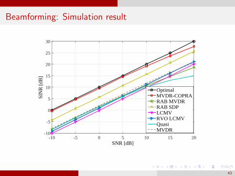
Beamforming: Simulation result
SNR [dB]-10 -5 0 5 10 15 20
SIN
R [
dB]
-10
-5
0
5
10
15
20
25
30
OptimalMVDR-COPRARAB MVDRRAB SDPLCMVRVO LCMVQuasiMVDR
43

Conclusion of Part I
We proposed a new regularization approach for linear least-squareproblems based on allowing a bounded perturbation into the lineartransformation matrix.
We chose the perturbation bound based on the MSE criteria and as aresult, the proposed approach minimizes the MSE approximately.
The solution of the proposed approach characteristic equation doesnot require knowledge of the signal and noise statistics.
Solution performs well compared to other methods over a wide SNRrange.
The proposed approach is shown to have the lowest run time.
44

Regularized Least Squares for Massive MIMO:Precise Analysis and Optimal Tuning
Joint work with Ismail Atitallah, Ayed Alrashdi , and & Christos Thrampoulidis
45

MIMO System model: AWGN channel
y = Ax0 + z
y ∈ Rm is the measurement vector at the receive antennas.
A ∈ Rm×n is the channel matrix, with iid Gaussian entries, with zeromean and variance 1
n .
x0 ∈ −1, 1n is a BPSK signal.
z ∈ Rm is a additive white Gaussian noise vector with variance σ2z
⇒ SNR= 1σ2z
.
δ = mn is the ratio of the number of receive/transmit antennas.
Optimum Receiver: Maximum Likelihood:
xML = arg minx∈−1,1n
‖Ax− y‖
⇒ computationally prohibitive in a massive MIMO context
46

MIMO System model: AWGN channel
y = Ax0 + z
y ∈ Rm is the measurement vector at the receive antennas.
A ∈ Rm×n is the channel matrix, with iid Gaussian entries, with zeromean and variance 1
n .
x0 ∈ −1, 1n is a BPSK signal.
z ∈ Rm is a additive white Gaussian noise vector with variance σ2z
⇒ SNR= 1σ2z
.
δ = mn is the ratio of the number of receive/transmit antennas.
Optimum Receiver: Maximum Likelihood:
xML = arg minx∈−1,1n
‖Ax− y‖
⇒ computationally prohibitive in a massive MIMO context46

Low-Complexity Receivers (1)
Two-step implementation of low-complexity receivers:
Solve a convex optimization.Hard-threshold.
Examples of common low-complexity receivers:
Least Squares (LS), aka Zero-Forcing receiver,
xLS = arg minx∈Rn
‖Ax− y‖2 = (ATA)−1ATy,
x∗LS = sign(xLS).
Regularized Least Squares (RLS),
xRLS = arg minx∈Rn
‖Ax− y‖2 + λ‖x‖2 = (ATA + λI)−1ATy,
x∗RLS = sign(xRLS).
Matrix inversion ⇒ the complexity is cubic.
47

Low-Complexity Receivers (1)
Two-step implementation of low-complexity receivers:
Solve a convex optimization.Hard-threshold.
Examples of common low-complexity receivers:
Least Squares (LS), aka Zero-Forcing receiver,
xLS = arg minx∈Rn
‖Ax− y‖2 = (ATA)−1ATy,
x∗LS = sign(xLS).
Regularized Least Squares (RLS),
xRLS = arg minx∈Rn
‖Ax− y‖2 + λ‖x‖2 = (ATA + λI)−1ATy,
x∗RLS = sign(xRLS).
Matrix inversion ⇒ the complexity is cubic.47

Low-Complexity Receivers (2)
RLS with Box Relaxation Optimization (RLS-BRO)
xBRO = arg minx∈[−1,1]n
‖Ax− y‖+ λ‖x‖2,
x∗BRO = sign(xBRO).
No closed-form expressionquadratic program ⇒ the complexity is also cubic.
Aim:
Derive precise BER expressionFind optimum regularizer λFind optimum Box threhsold
48

Relevant literature
BER := 1n
∑ni=1 1x∗i 6=x0,i.
Receiver BER approach Reference
LS Exact Exact non-asymptotic formula, e.g. Tse and Viswanath 1
RLS RMT Tulino and Verdu 2
LS-BRO CGMT Thrampoulidis and Hassibi3
RLS-BRO CGMT This Talk
RMT: Random Matrix TheoryCGMT: Convex Gaussian Min-max Theorem
49

Asymptotic BER Analysis
LS: limn→∞ BERLS = Q ((δ − 1)snr) , (for δ > 1).
RLS: limn→∞ BERRLS = Q
(√δ− 1
(1+Υ(λ,δ))2(Υ(λ,δ)
1+Υ(λ,δ)
)2+ 1
snr
), where
Υ(λ, δ) =1−δ+λ+
√(1−δ+λ)2+4λδ
2δ.
The optimal λ that minimizes the asymptotic BERRLS
is 1SNR
⇒ LMMSE receiver is also optimal in the BER sense.
A high SNR approximation of the BER of LMMSE is
Q((δ − 1 + 1
(δ−1)SNR
)SNR
)' Q((δ − 1)SNR).
50

Convex Gaussian Min-max Theorem
Convex-Gaussian Min-Max Theorem (CGMT)
aConsider the following two min-max problems:
Primary Optimization (PO) Problem: Φ(G) := minw∈Sw
maxu∈Su
uTGw + ψ(w,u)
Auxilary Optimization (AO) Problem: φ(g,h) := minw∈Sw
maxu∈Su
‖w‖gTu− ‖u‖hTw + ψ(w,u)
ψ is convex-concave.
wΦ any optimal minimizers in the (PO).
wφ any optimal minimizers in the (AO).
Then, if limn→∞ Pr(wφ ∈ S) = 1, it also holds limn→∞ Pr(wΦ ∈ S) = 1.
aC. Thrampoulidis, E. Abbasi and B. Hassibi “Precise error analysis of regularizedM-estimators in high-dimensions”- arXiv preprint arXiv:1601.06233, 2016
We apply the CGMT to the set in which the BER concentrates, i.e.
S =w; |BER− E[BER]| < ε
. (26)
51

Precise Bit Error Rate (BER) Analysis
Theorem (BER of RLS-BRO)
As n,m→∞, such that mn→ δ ∈ (0,∞), it holds in probability
limn→∞
BERBRO = Q(1
τ∗),
where τ∗ is the unique solution to the following
minτ>0
maxβ>0
D(τ, β) : = δτβ +β
SNRτ− λβ2
2+
4β
τQ
(2
τ+
2
β
)− 4βp
(2
τ+
2
β
)− β2
βτ
+ 2
∫ 2β
− 2β− 2τ
(h− 2
β
)2
p(h)dh.
τ∗ can be efficiently computed by writing the first order optimality conditions, i.e.∇(τ,β)D(τ, β) = 0.
τ∗ (and hence the BER) depends on δ = mn
, SNR and the regularizer λ.
52

Optimal tuning of the Regularizer
0 5 10 150
1
2
3
10 log10(snr)
λB
RO
∗
1snr
δ = 0.5
δ = 1
δ = 1.5
δ = 2
The optimal regularizer λBRO∗ is an decreasing function of the ratio m
n.
It is always below 1SNR
.
∃snr ∈ R+, such that, λBRO∗ = 0 for all snr ∈ (snr,∞).
53

LMMSE vs RLS-BRO
0 5 10 1510−5
10−4
10−3
10−2
10−1
100
10 log10(snr)
BE
R
RLS-BRO: δ = 0.7
LMMSE: δ = 0.7
RLS-BRO: δ = 1
LMMSE: δ = 1
simulations
Figure: n = 500.
Recall the following high-SNR approximations:limn→∞BERBRO ' Q((δ − 1
2)snr)
limn→∞BERRLS ' Q((δ − 1)snr)54

Is [−1, 1] the optimal relaxation interval?
xBRO = arg minx∈[−t,t]n
‖Ax− y‖+ λ‖x‖2
x∗BRO = sign(xBRO)
In a similar fashion, we can prove that limn→∞ BERBRO = Q(
1τ∗
), where
τ∗ = arg minτ>0 maxβ>0 D(τ, β; t, λ, δ, SNR).
τ∗(t, λ, δ, SNR) is a function of SNR, the sampling ratio δ, the regularizer λ andthe relaxation threshold t.We select the optimal relaxation threshold t∗, and the optimal regularizer λ∗, suchthat:
(t∗, λ∗) ∈ argmin(t,λ)∈R2
+
τ∗(t, λ, δ, SNR)
55

Joint optimization of the regularizer and the relaxationthreshold
0 5 10 150.75
0.8
0.85
0.9
0.95
1
10 log10(snr)
Op
tim
alre
laxa
tion
thre
shol
d
δ = 0.7
δ = 1
0 5 10 150
1
2
3
10 log10(snr)
λB
RO
∗
1snr
δ = 0.7
δ = 1
56

What if we don’t know the SNR?
If the signal and noise variances are not known, we use the expression of the costfunction of RLS to estimate the SNR, to ultimately allow for an optimal tuning of theregularizer. Let J(σ2
x, σ2z) denote the asymptotic cost function of RLS.
J(σ2x, σ
2z , λ, δ) := lim
n→∞minx‖Ax− y‖2 + λ‖x‖2.
= a(λ, δ)σ2x + b(λ, δ)σ2
z ,
where
a(λ, δ) =
(δλ
Υ− λ2
Υ2− λ
Υ + Υ2
)(Υ2
δ(1 + Υ)2 − 1
)− λΥ
1 + Υ+ λ,
b(λ, δ) =
(δλ
Υ− λ2
Υ2− λ
Υ + Υ2
)((1 + Υ)2
δ(1 + Υ)2 − 1
)+λ
Υ,
and
Υ =1− δ + λ+
√(1− δ + λ)2 + 4λδ
2δ.
57

What if we don’t know the SNR?
0 1 2 3 4 5 6 70
0.1
0.2
0.3
0.4
0.5
0.6
λ
J(x
RL
S)
Theoretical
Empirical
Figure: m = 500, n = 800, σ2x = 1 and
σ2z = 0.3.
−10 0 10 20 30−10
0
10
20
30
10 log10(SNR)
SN
Rin
dB
True SNR
Estimated SNR
Figure: m = 500, n = 800 andσ2x = 1.
Use one observation y to estimate the SNR.
Use the SNR estimate to set the regularization parameter λ and the box thresholdt.
58

SNR Estimation under Correlation
59
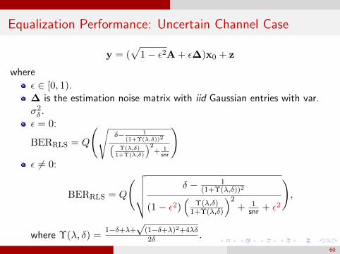
Equalization Performance: Uncertain Channel Case
y = (√
1− ε2A + ε∆)x0 + z
where
ε ∈ [0, 1).∆ is the estimation noise matrix with iid Gaussian entries with var.σ2δ .ε = 0:
BERRLS = Q
(√δ− 1
(1+Υ(λ,δ))2(Υ(λ,δ)
1+Υ(λ,δ)
)2+ 1
snr
)ε 6= 0:
BERRLS = Q
(√√√√√ δ − 1(1+Υ(λ,δ))2
(1− ε2)(
Υ(λ,δ)1+Υ(λ,δ)
)2+ 1
snr + ε2
),
where Υ(λ, δ) =1−δ+λ+
√(1−δ+λ)2+4λδ
2δ .
60

Equalization Performance: Uncertain Channel Case
-5 0 5 10 15
SNR (dB)
10 -5
10 -4
10 -3
10 -2
10 -1
100
BE
R
RLS: = 0RLS: = 0.1Simulations
Figure: BER performance δ = 1.3, n = 256
[4] Ayed M. Alrashdi, Ismail Ben Atitallah, Tareq Y. Al-Naffouri and Mohamed-Slim Alouini “Precise Performance Analysis ofthe LASSO Under Matrix Uncertainties”, GlobalSIP, 2017.
61

Optimum Training
Given a power budget at the transmitter
We can use some for channel estimation (reduces ε).We can use some for data transmission (reduces BER).
Total Energy
E = Ep + Ed
= αE + (1− α)E
What is the optimum trade-off?
62
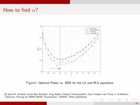
How to find α?
0 0.1 0.2 0.3 0.4 0.5 0.6 0.7 0.8 0.9 110 -4
10 -3
10 -2
10 -1
100
BE
R
RLS-TheoryRLS-SimulationLS-TheoryLS-Simulation
*
Figure: Optimal Power vs. BER for the LS and RLS equalizers.
[5] Ayed M. Alrashdi, Ismail Ben Atitallah, Tarig Ballal, Christos Thrampoulidis, Anas Chaaban and Tareq Y. Al-Naffouri“Optimum Training for MIMO BPSK Transmission”, SPAWC, 2018 (submitted).
63
Conclusion of Part II
Precise Asymptotic BER analysis of the Box Relaxation Optimizationfor BPSK signal recovery, that allow efficient optimal tuning of theparamters.
Tuning is possible even if SNR is not known as we are able toestimate it precisely.
Analysis is extended to the case where channel exhibits uncertainty.
Analysis used to find optimize training power to minimize SNR.
Future work: We are extending the work to other constellations(PAM, QAM), other equalizers, and correlated channel case.
64

Thank you
65

Through Inspiration, Discovery King Abdullah University of Science and Technology

What is KAUST?
• Graduate Level research university governed by an independent Board of Trustees
• Merit based, open to all from around the world
• Research Centers as primary organizational units
• Research funding and collaborative educational programs
• Collaborative research projects, linking industry R&D and economic development
• Environmentally responsible campus

An iconic part of campus, the Campus Library is more than just a place to house periodicals. This contemporary building encased in translucent stone engages light to create a tranquil space for people to gather, think, and learn. It’s distinctive architecture won the 2011 AIA/ALA Library Building Award given by the American Institute of Architects (AIA) and the American Library Association (ALA).

The Student Center is a one-stop spot for many student-related services to support academic, personal, and professional development.