Three Essays on Debt

Lijun Wang

Submitted in partial fulfillment of therequirements for the degree of

Doctor of Philosophyin the Graduate School of Arts and Sciences

COLUMBIA UNIVERSITY

2020

c© 2019Lijun Wang

All Rights Reserved

ABSTRACT

Three Essays on Debt

Lijun Wang

This dissertation contains three essays on debts of different forms that make con-

tributions to the areas of international macroeconomics and spatial economics. In

particular, the first two essays study sovereign debts. They examine sovereign de-

fault behaviors together with interactions between sovereign defaults and countries’

costs of borrowing. The third essay looks at bank loans. It explores the possibility

of understanding economic agglomeration through distance-related financial frictions

firms face when borrowing from banks.

Contents

List of Figures ii

List of Tables iii

Acknowledgements iv

Preface 1

Chapter I. Defaultable Sovereign Debts under Plausible Risk-Averse Pricing 4

Chapter II. The Home Bias of Sovereign Borrowing 20

Chapter III. The Financial Channel of Economic Agglomeration 40

Bibliography 58

Appendix 67

i

List of Figures

I-1 Model vs. Data — Argentina 2001 Default Episode . . . . . . . . . . . 5

II-1 Historical Default Episodes . . . . . . . . . . . . . . . . . . . . . . . . 24

II-2 Equilibrium Bond Prices qd, qe at Mean Output y . . . . . . . . . . . . 34

III-1 Parallel Pre-Trend in Bank Loan Originations . . . . . . . . . . . . . . 52

III-2 Parallel Pre-Trend in Establishment Count Growth . . . . . . . . . . . 53

A-1 Benchmark Model Numerical Solutions . . . . . . . . . . . . . . . . . . 68

A-2 M∗t+1 Process Before and After Adjustments . . . . . . . . . . . . . . . 71

A-3 Robustness Simulations in Neighboring Specifications . . . . . . . . . . 72

A-4 Historical Default Episodes with Hyper-Inflations . . . . . . . . . . . . 73

A-5 Top Serial Defaulters . . . . . . . . . . . . . . . . . . . . . . . . . . . . 74

A-6 U.S. Economic Density at County-Level . . . . . . . . . . . . . . . . . 76

A-7 U.S. Economic Density at County-Level and Banks . . . . . . . . . . . 76

A-8 Map of County-Level Bank Footprints . . . . . . . . . . . . . . . . . . 77

ii

List of Tables

I-1 Benchmark Calibration & Solution Algorithm Parameters . . . . . . . 14

I-2 Benchmark Simulations vs. Data — Argentine Credit Spread . . . . . 15

I-3 Plausible Risk-Averse Pricing Calibration and Simulation . . . . . . . 18

II-1 Model Counterfactual Calibration Parameters . . . . . . . . . . . . . . 33

II-2 Regressions of Domestic Debt Shares on netInflow Openness . . . . . . 37

III-1 Sample Summary Statistics . . . . . . . . . . . . . . . . . . . . . . . . 49

III-2 Diff-in-Diff Regression Results on Loan Originations . . . . . . . . . . 55

III-3 Diff-in-Diff Regression Results on Establishment Growth . . . . . . . . 56

iii

Acknowledgements

First and foremost, I would like to thank my primary advisor, Patrick Bolton, for his

continuous support in whatever endeavor I chose to pursue — both academically and

professionally. It is his advice that has led me through the most doubtful moments

when completing this work and even beyond. In the meanwhile, I have also received

many helpful feedbacks and guidance from Donald Davis, Andres Drenik, Matthieu

Gomez, Harrison Hong, Reka Juhasz, Emi Nakamura, Ailsa Roell, Jose Scheinkman,

Stephanie Schmitt-Grohe, Jon Steinsson, Joseph Stiglitz, Martin Uribe, and David

Weinstein. I am tremendously grateful for their help in making this work better.

I would also like to thank seminar participants at Columbia from the past five

years, including but not limited to those from Financial Economics Colloquium, Inter-

national Trade Colloquium, Economic Fluctuations Colloquium, and Monetary Eco-

nomics Colloquium. I have benefitted a lot from their constructive suggestions and

comments during my presentations. Some of them have also generously allocated their

time to initiate intellectual discussions with me on my research, and I am thankful

to them.

I appreciate funding support from the Department and the University, adminis-

iv

trative support from our Ph.D. Program Coordinators — Amy Devine and Shane

Bordeau (in reverse order of their appointments), and other logistical support from

our Directors of Graduate Studies — Navin Kartik, Jon Steinsson and Brendan

O’Flaherty (in reverse order of their appointments). Without them, I would have

run into a lot more bumps while completing this work.

I also wish to acknowledge various data sources that have made this research

possible — Census Bureau, Federal Deposit Insurance Corporation (FDIC), Fed-

eral Financial Institutions Examination Council (FFIEC), Federal Reserve Bank of

Chicago (FRB Chicago), Missouri Census Data Center (MCDC), National Bureau

of Economic Research (NBER), National Historical Geographic Information System

(NHGIS), and Wharton Research Data Services (WRDS). While analyzing these data,

I relied tremendously on computational tools, including MATLAB, QGIS, STATA,

and Yeti High-Performance Computing (HPC) Cluster at Columbia. All remaining

errors are my own.

Last but not least, staffs at the Graduate School of Arts and Sciences (GSAS)

Writing Studio have been an invaluable help to perfecting writing for my work. I want

to thank them for their patience with many versions of my drafts in this process.

v

To my wife,

Amy,

who has kept me company

in this marathon of the mind.

vi

Preface

Economic agents use debt as a vehicle for external financing in different contexts.

Households take on debts such as credit card balances to finance daily spendings,

firms take on debts such as bank loans to finance productions and investments, and

governments take on debts such as sovereign bonds to finance public operations and

programs.

This dissertation contains three essays on debts of different forms that make con-

tributions to the areas of international macroeconomics and spatial economics. In

particular, the first two essays study sovereign debts. They examine sovereign de-

fault behaviors together with interactions between sovereign defaults and countries’

costs of borrowing. The third essay looks at bank loans. It explores the possibility

of understanding economic agglomeration through distance-related financial frictions

firms face when borrowing from banks.

Chapter 1 is titled Defaultable Sovereign Debts under Plausible Risk-Averse Pric-

ing. It addresses an asset-pricing anomaly in structural sovereign default models.

When calibrated to match historical default probabilities, these models imply a level

of sovereign bond credit spread that is too low to be commensurate with data. One

1

line of research attempts to improve the model by building an extension of risk-

averse investors into it; however, such efforts have not entirely resolved the problem.

Rather than making another attempt in this direction, chapter 1 takes a step back

and examines the feasibility of this entire approach. Can any plausible extension of

risk-averse investors into the standard model resolve the low-spread anomaly? If not,

it is meaningless trying to build one in the first place.

To be precise, chapter 1 deems an investor extension plausible as long as it implies

an investor pricing behavior that does not allow arbitrage relative to existing bonds

in this market. However, by incorporating a pricing kernel that is consistent with the

“market price of risk” in the data (and hence leaving no room for arbitrage), the low-

spread anomaly in sovereign default models can barely be improved. Relying on this

result, chapter 1 concludes that no plausible extensions of risk-averse investors can

resolve the low-spread anomaly. To improve the structural sovereign default models

in this regard, we should look elsewhere for theoretical resolutions.

Chapter 2 is titled The Home Bias of Sovereign Borrowing. It looks at the is-

sue of domestic debt being missing from existing sovereign finance theories. Notably,

domestic debt accounts for nearly two-thirds of total sovereign borrowing, and yet ex-

isting theories remain completely agnostic on this and assume countries only borrow

externally. To properly account for both domestic and external debts in one theoret-

ical framework, what are the relevant trade-offs to consider? How does the “home

bias” arise? What is driving the cross-country heterogeneity in these behaviors?

To answer these questions, chapter 2 develops a novel general equilibrium model,

in which the benevolent government can strategically choose to borrow from domestic

2

or external markets. The model can generate the observed “home bias” in sovereign

borrowing as an equilibrium outcome through the government’s strategic financing

behaviors. By introducing a capital control constraint on foreign investments within

the domestic market, the model implies that looser inflow capital controls for a coun-

try are associated with a stronger home bias in its sovereign borrowing. Using a

cross-country dataset, chapter 2 also finds support for this association in the data.

Chapter 3 is titled The Financial Channel of Economic Agglomeration. It revis-

its a classic question of how economic agglomeration arises from a novel financial

perspective. Traditionally, urban economists interpret economic agglomeration as an

outcome of firms choosing to locate near each other, because doing so begets increas-

ing returns to scale in their productions. Alternatively, chapter 3 presents evidence

that explains economic agglomeration as a result of firms more likely emerging to-

gether near banks, because proximity to banks reduces frictions to obtain loans.

To show that a bank can cause firms to agglomerate in its proximity by easing

their financial frictions, chapter 3 carefully designs a natural experiment to examine

what a quasi-exogenous bank relocation does to the bank’s surroundings. A standard

difference-in-difference approach shows that relocation of a bank closer to a region

indeed causes more supply of bank loans in that region, and subsequently causes

more firm establishments to emerge and agglomerate within the same area. This

result supports the financial channel of economic agglomeration, and it also suggests

the importance of credit availabilities for regional economic growths.

Without further ado, we now begin expositions of the entire dissertation below.

3

Chapter I.

Defaultable Sovereign Debts under

Plausible Risk-Averse Pricing

There is an asset-pricing anomaly in structural models that examine sovereign defaults

among emerging economies (e.g., Eaton and Gersovitz, 1981; Arellano, 2008).1 When

calibrated to match historical default probabilities, these models imply a level of

sovereign bond credit spread that is too low to be commensurate with data.2

For a quick illustration, one such model is calibrated to match the Argentine

economy per Arellano (2008) in Figure I-1. Given a fitted output process, the model

can predict the observed sovereign default around 2001. For the years leading up to

1Eaton and Gersovitz (1981) make a seminal contribution to modeling sovereign defaults. Byintroducing debt market exclusion for countries in default, they present a stylized model to analyzesovereign defaults as a country’s strategic choices. Arellano (2008) later develops this approach intoa full-fledged structural model, which one can calibrate for quantitative simulations.

2There is another strand of literature that explicitly studies sovereign bond yields and creditspreads (e.g., Duffie and Singleton, 1999; Duffie, Pedersen, and Singleton, 2003). Unlike thosestructural sovereign default models mentioned above, this literature treats sovereign defaults asexogenous credit events.

4

Figure I-1: Model vs. Data — Argentina 2001 Default Episode

(Vertical Axis: Left - Percentage, Right - Log Deviations)

1994Q1 1995Q1 1996Q1 1997Q1 1998Q1 1999Q1 2000Q1 2001Q1 2002Q10

5

10

15

20

25

30

35

40

-0.15

-0.1

-0.05

0

0.05

0.1

0.15

Argentina and Model Time Series

Output (right axis)

Trade Balance (right axis)

Spread

DataModel

the default, it also successfully simulates the observed dynamics in macroeconomic

variables such as the trade balance. However, the model implies a time series of

Argentine bond credit spread3 that is too low to be comparable with its empirical

counterpart.4

3The model defines the credit spread as the interest rate at which the Argentine government isborrowing, less the international risk-free interest rate benchmark. Its empirical counterpart is theprevailing interest rate at which the Argentine government is borrowing, less the 5-year U.S. bondyield.

4Yue (2010) shows that model-implied credit spread becomes even lower when she incorpo-rates post-default debt recoveries into the standard model. In her set-up, the model’s asset-pricingperformance is even more problematic.

5

To resolve this low-spread anomaly, one line of research attempts to improve the

model by building an extension of risk-averse investors into it, hence replacing the

current risk-neutral pricing set-up.5 By doing so, bond investors in the model can

charge, on top of actuarially fair compensations, an additional premium for bearing

default risks. This idea also finds empirical support. Longstaff et al. (2011) study an

extensive set of sovereign CDS data and find that the risk premium indeed accounts

for a significant portion of the sovereign bond credit spread.6

A few attempts have been made to extend the model in this direction, result-

ing in minimal success. Lizarazo (2013) introduces bond investors whose preferences

exhibit decreasing absolute risk aversion (DARA). In her model, the wildest param-

eter assumptions can only resolve nearly half of the low-spread anomaly. Uribe and

Schmitt-Grohe (2017) bring U.S. household investors with constant relative risk aver-

sion (CRRA) utilities into the model. However, this set-up can barely improve the

low-spread anomaly across all parameter specifications.

Rather than making another attempt in this direction, chapter 1 takes a step back

and examines the feasibility of this entire approach. Can any plausible extension

of risk-averse investors into the model resolve the low-spread anomaly? If not, it is

meaningless trying to build one in the first place. This question is challenging because

5Alternatively, another line of research by Chatterjee and Eyigungor (2012) and Arellano andRamanarayanan (2012) builds an extension of debt maturity structures into the model, hence re-placing the current one-period bond set-up. These efforts have proven helpful in improving themodel’s asset-pricing performance. On a side note, Garcia-Schmidt (2015) introduces asymmetricinformation on debtor country incomes between bond investors and debtor countries. The idea isto see if adverse selection by bond investors increases the credit spread to a level that resolves themodel’s asset-pricing anomaly. However, this approach achieves very minimal quantitative success.

6Longstaff et al. (2011) find that “[o]n average, the risk premium represents about a third ofthe credit spread” in sovereign bonds.

6

it aims to make a statement on not one but all possible extensions that are plausible.

However, being plausible sounds vague and subjective. What exactly does it

mean when we use it to describe an extension of risk-averse investors into the model?

To clarify, chapter 1 deems an investor extension plausible as long as it implies an

investor pricing behavior that is consistent with the “market price of risk” in the

data. In other words, an equivalent way of asking the question is: can we resolve the

low-spread anomaly by introducing risk-averse investors who price risk in a way that

does not allow arbitrage with existing bonds in this market?

To introduce such risk-averse pricing behaviors into the standard model, chapter 1

uses directly the investors’ stochastic discount factor (SDF, or equivalently the pricing

kernel, denoted as Mt+1). Doing so has three advantages. First, it abstracts away

from specific economic models7 of risk-averse investors while pricing bonds.8 Second,

it adapts to the standard sovereign default model without compromising tractability

in modeling sovereign defaults (Arellano, 2008). Third, it is possible to construct a

risk-averse pricing kernel that is plausible per our discussions above (Cochrane and

Piazzesi, 2005).

To construct a pricing kernel that is arbitrage-free relative to existing bonds in

the market, we follow an algebraic procedure in Cochrane and Piazzesi (2005), who

use prices and forward rates on one- through five-year zero-coupon U.S. government

7Existence of the SDF does show that there is an economic model that implies a pricing behaviorconsistent with the SDF; however, an examination of the SDF does not quickly lead one to the correcteconomic model. Hansen and Jagannathan (1991) have performed such an inquiry on discountfactors for stocks.

8Recall that the SDF prices risk based on the law of one price and the condition of no-arbitrage

via the primitive pricing equation P(n)t = Et(Mt+1Mt+2...Mt+n−1), in which P

(n)t denotes the

period-t price of a discount bond that returns 1 unit of consumption in n periods.

7

bonds. Notably, running forecasting regressions of excess bond returns on a combina-

tion of forward rates, they find unprecedented forecastability (with R2 up to 0.44).9

To account for this forecastability while modeling how investors price risk in these

bonds, they algebraically derive a pricing kernel that leaves no room of arbitrage

relative to the included bonds in those regressions. It is this kernel we now introduce

into the standard sovereign default model as the plausible risk-averse pricing kernel

(denoted as M∗t+1).10

With the plausible risk-averse pricing kernel, the model yields only minimal im-

provements on its simulated credit spread. Again, for the years leading up to the

2001 Argentine default episode, the standard model implies an average credit spread

of 3.39%, while the model with the plausible risk-averse pricing kernel yields an aver-

age credit spread of 3.65%. Despite the 0.26 percentage point increase, the observed

Argentine bond credit spread for the same period has an average of an unreachable

10.25%. These results suggest that no plausible extensions of risk-averse investors

into the model could satisfactorily resolve the low-spread anomaly. To improve the

model’s asset-pricing performance, we should look elsewhere for theoretical resolu-

tions.

This chapter organizes itself as follows. Section A outlines a benchmark sovereign

default model with risk-neutral pricing per Arellano (2008). Section B modifies the

model to introduce risk-averse pricing via the SDF framework. Section C constructs

9Also, see Campbell and Shiller (1991) and Fama and Bliss (1987) for earlier work on this matter.

10One implicit assumption in applying M∗t+1 here is that investors on emerging market sovereign

bonds also have access to these zero-coupon U.S. government bonds and the associated forwardcontracts; otherwise, being arbitrage-free relative to these bonds does nothing in restricting pricingbehaviors.

8

the plausible risk-averse pricing kernel M∗t+1 and adapts it into the model. Finally,

section D concludes the chapter.

A. Benchmark Model with Risk-Neutral Pricing

The benchmark model closely follows Arellano (2008). It is a dynamic stochastic

general equilibrium model containing a continuum of households, risk-neutral inter-

national investors, and a benevolent government.

Households solve a standard inter-temporal consumption problem. Their repre-

sentative agent receives a Markov stochastic stream of tradable consumption goods

yt that follows a transition function f (yt+1, yt) and has compact support Y .11 Its

objective is to maximize its expected lifetime utility, and in doing so, it chooses its

consumption ct in each period.

Formally, households try to

max{ct}

+∞∑t=0

βtE0 [u (ct)] ,

subject to their inter-temporal budget constraint that takes shape after the govern-

ment makes its borrowing and default decisions each period. β ∈ (0, 1) denotes the

households’ subjective period discount factor. u(ct) denotes the households’ period

utility function. It takes a standard constant relative risk aversion (CRRA) utility

functional form u (ct) =c1−σt −1

1−σ , in which σ denotes the households’ coefficient of

11In other words, yt ∈ Y,∀t.

9

relative risk aversion.

Households borrow from the international financial market through their govern-

ment via its issued sovereign bonds. If the government is not in default of its bonds,

households’ budget constraint is

ct = yt +Bt − qtBt+1,

in which Bt is the nominal value of previously issued bonds households have to repay

in period t, Bt+1 is the nominal value of bonds due next period, and qt is the current-

period price for each nominal unit of bonds due next period.12

If the government is in default, prior debt contracts are no longer honored (i.e.,

Bt = 0), and the debtor country is temporarily excluded from the international

financial market (i.e., Bt+1 = 0). In this case, households follow a simple hand-to-

mouth budget constraint

ct = ydeft ,

in which they consume everything from their endowment income ydeft . ydeft denotes

the period endowment income during a default; it is assumed to be a depressed level

of yt because sovereign default imposes output costs on the debtor country.

International investors are risk-neutral. As long as they are compensated with

an expected return at the constant international lending rate rf > 0, they can borrow

or lend as much as they need to.

12A positive Bt+1 means the debtor country saves qtBt+1 in the current period t and receivesBt+1 in period t+ 1. A negative Bt+1 means the debtor borrows qt (−Bt+1) in the current period,and pays back, conditioning on non-default, (−Bt+1) in period t+ 1.

10

With perfect information on the debtor country income process, investors price

the defaultable bonds in a risk-neutral manner so that they break even in expected

value in every bond contract. Formally, taking bond prices qt as given in every period,

lenders choose loans Bt+1 to maximize expected profits Φt = qtBt+1 − 1−δt+1

1+rfBt+1, in

which δt+1 denotes the expected probability of debtor country default in period t+ 1.

This requires bond prices qt to satisfy the risk-neutral pricing equation (I..1):

qt =1− δt+1

1 + rf. (I..1)

The next-period default risk δt+1 is endogenous to the model. It depends on

the government’s incentives to default under different possible yt+1 realizations. In

equilibrium, it is the sum of probabilities for yt+1 realizations in the next period, in

which the government finds it optimal to default. Formally,

δt+1 =

∫D(Bt+1)

f (yt+1, yt) dyt+1,

in which D(Bt+1) ≡ {yt+1 ∈ Y : government finds it optimal to default on Bt+1}.13

Using the endogenous discount bond price qt, the model defines the interest rate

at which the government is borrowing using its reciprocal 1 + rt = 1qt

. Following this,

the credit spread of the defaultable bonds r∆t is defined as r∆

t ≡ 1qt− (1 + rf ).

The benevolent government solves a strategic borrowing and default problem on

behalf of households in this economy. Entering each period, it observes its current-

13A formal introduction of D(Bt+1) is deferred until expositions on the government’s strategicdefault problem.

11

period income yt, and decides whether to repay on its maturing debts Bt. If it does,

it continues to borrow by selling bonds with face value Bt+1 at a unit price of qt, and

rebates all proceeds back to the households in lump-sum transfers. If not, it declares

a default. Maturing debts Bt are ignored but no new bonds could be issued.

Being in default has two consequences in this model — temporary financial ex-

clusion and direct output loss. First of all, the debtor country loses its access to

the international financial market and only re-enters with an exogenous probability

θ ∈ [0, 1) during each subsequent period. Secondly, its output remains at a depressed

level ydeft . ydeft is assumed to be a concave piecewise liner function with a kink at

a threshold y, which denotes the maximum output level receivable by the debtor

country while it is in default. Formally, ydeft = min{y, yt}.

The government’s strategic borrowing and default problem is outlined below. (For

brevity of notations, I drop all t−subscripts and replace t + 1 notations with ′ vari-

ables.) Entering each period, the government is maximizing its welfare value function

vo (B, y) by choosing between continuing to repay debts vc(B, y) and declaring default

vd(y),

vo (B, y) = max{vc,vd}

{vc (B, y) , vd (y)

}.

The value function of continuing repayments vc (B, y) is

vc (B, y) = maxB′

{u (y − q (B′, y)B′ +B) + β

∫y′vo (B′, y′) f (y′, y) dy′

},

12

and the value function of declaring default vd (y) is

vd (y) = u(ydef

)+ β

∫y′

[θvo (0, y′) + (1− θ) vd (y′)

]f (y′, y) dy′.

The choices between vd (y) and vc (B, y) constitute the government’s default policy

set D(B). Formally, D(B) ≡ {y ∈ Y : vd (y) > vc (B, y)}. In correspondence, the

government’s repayment policy set is A(B) ≡ {y ∈ Y : vd (y) ≤ vc (B, y)}.

With the households, the international investors, and the government in place, we

now define the recursive equilibrium in this economy.

Definition. The recursive equilibrium in this economy is formally defined as the

policy functions/sets {ct}+∞0 , D(B), {Bt+1}+∞

0 , and market prices {qt}+∞0 such that

1. households maximize their expected lifetime utility subject to their budget con-

straint, taking as given the government policies;

2. the government default policies and borrowing choices satisfy its optimization

problem, taking as given the endogenous prices for their bonds;

3. endogenous bond prices reflect corresponding default probabilities, and are con-

sistent with international investors’ expected zero profits condition,

taking as given the stochastic endowment process {yt}+∞0 .

To be able to use the model for simulations, we first need to solve for its equilib-

rium solutions, using a calibration matched to the simulated empirical episode. For

instance, we now simulate the Argentina 2001 default episode as in Figure I-1.

13

First, we start by calibrating the model to Argentina. The goal of the calibration

is to have the model predict an equilibrium sovereign default at about 3% annualized

probability — an observed default probability in Argentina at the annual frequency,

while we assume its income process follows a demeaned log AR(1), ln yt+1 − ¯ln y =

ρ(ln yt − ¯ln y

)+ ηεt+1, in which ¯ln y = ln 10 and εt+1 is a standard white noise. Table

I-1 outlines all parameters for the calibration in its top panel.

Table I-1: Benchmark Calibration & Solution Algorithm Parameters

Variables Parameters Source

Risk-free interest rate rf = 1.7% 5-year U.S. bond quarterly yield

HH risk aversion σ = 2 standard

AR(1) for ln yt+1 ρ = 0.945, η = 0.025 Argentine quarterly GDP

Discount factor β = 0.953 Target 3% default prob.

Prob. of re-entry θ = 0.282 Argentine historical re-entry prob.

Depressed output y = 0.969E (y) ,E(y) = 10 Target 3% default prob.

Grid for B [−3.475, 1.5], equally spaced standard

Grid for y discretized AR(1) Tauchen-Hussey algorithm

No. of grid points for B 200

No. of grid points for y 21

Convergence criterion 10−8

Maximum iterations 5000

Target Statistics

Default prob. 3.0% Argentine historical default prob.

We then proceed to computationally solve for equilibrium solutions using standard

value function iterations14 on discretized grids. Table I-1 outlines all parameters for

the solution algorithm in its second panel. For brevity of expositions, we plot the

numerical equilibrium solutions in Appendix A2. Overall, these solutions comply with

our intuition in that a higher debtor country income drives lower default probabilities,

which in turn increases bond prices and decreases the country’s cost of borrowing.

14See Appendix A1 for a detailed solution algorithm.

14

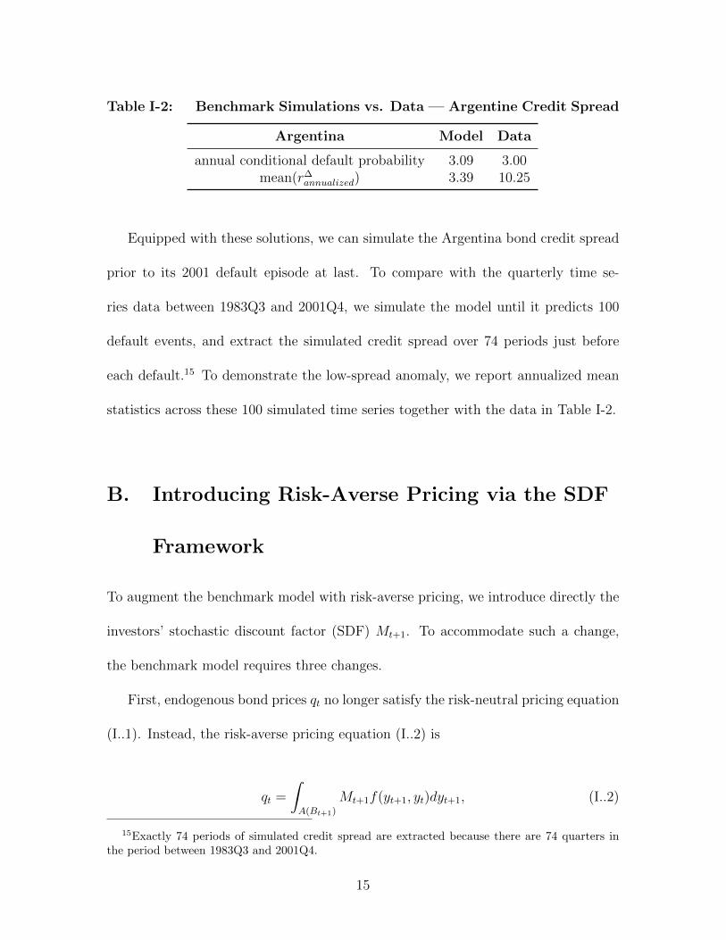
Table I-2: Benchmark Simulations vs. Data — Argentine Credit Spread

Argentina Model Data

annual conditional default probability 3.09 3.00mean(r∆

annualized) 3.39 10.25

Equipped with these solutions, we can simulate the Argentina bond credit spread

prior to its 2001 default episode at last. To compare with the quarterly time se-

ries data between 1983Q3 and 2001Q4, we simulate the model until it predicts 100

default events, and extract the simulated credit spread over 74 periods just before

each default.15 To demonstrate the low-spread anomaly, we report annualized mean

statistics across these 100 simulated time series together with the data in Table I-2.

B. Introducing Risk-Averse Pricing via the SDF

Framework

To augment the benchmark model with risk-averse pricing, we introduce directly the

investors’ stochastic discount factor (SDF) Mt+1. To accommodate such a change,

the benchmark model requires three changes.

First, endogenous bond prices qt no longer satisfy the risk-neutral pricing equation

(I..1). Instead, the risk-averse pricing equation (I..2) is

qt =

∫A(Bt+1)

Mt+1f(yt+1, yt)dyt+1, (I..2)

15Exactly 74 periods of simulated credit spread are extracted because there are 74 quarters inthe period between 1983Q3 and 2001Q4.

15

in which Mt+1 measures how much investors value one unit of next-period consump-

tion in the current period. Intuitively, qt is the sum of discounted future pay-offs

coming from bonds if there is no default.

Second, the risk-free interest rate rft is now time-changing as well. By the same

token, the risk-free interest rate rft satisfies

1 = (1 + rft )

∫Mt+1f(yt+1, yt)dyt+1,

which intuitively says the current-period risk-free yield has to enable a risk-free pay-off

of one unit of future consumption across all possible states. Subsequently, the credit

spread of defaultable bonds r∆t ≡ 1

qt− (1 + rft ) in this framework correspondingly

translates into r∆t = 1∫

A(Bt+1)Mt+1f(yt+1,yt)dyt+1

− 1∫Mt+1f(yt+1,yt)dyt+1

.

Third, the exogenous stochastic structure for the economy is now a joint process

between Mt+1 and yt+1

ln yt+1 − ¯ln y

Mt+1 − M

=

ρy 0

0 ρM

ln yt − ¯ln y

Mt − M

+

ηy 0

0 ηM

εyt+1

εMt+1

,

in which E[εyt+1] = E[εMt+1] = 0, and E[(εyt+1)2] = E[(εMt+1)2] = 1. This is assuming

Mt+1 and yt+1 are two independent stochastic processes. Intuitively, this is to say that

the debtor country is too small to affect pricing behaviors on international creditors

in the rest of the world, and the pricing kernel Mt+1 is independent of economic

conditions in the debtor country.

16

C. Adapting a Plausible Risk-Averse SDF

To construct a pricing kernel that is arbitrage-free relative to existing bonds in the

market, we follow an algebraic procedure in Cochrane and Piazzesi (2005), who use

prices and forward rates on one- through five-year zero coupon U.S. government

bonds.

Formally, the plausible risk-averse pricing kernel M∗t+1 is constructed as

M∗t+1 = exp(−y(1)

t −1

2λTt Σλt − λT

t εt+1),

in which t denotes a month, y(1)t denotes the log yield of one-year discount bond,

λt, Σ, and εt+1 are mathematical constructs from pre-defined forecasting regressions.

These regressions are specified as

rxt+1 = βft + εt+1; cov(εt+1ε

Tt+1

)= Σ,

in which excess log returns rxt+1 ≡ [ rx(2)t+1 rx

(3)t+1 rx

(4)t+1 rx

(5)t+1

]T and log forward

rates ft ≡ [ 1 y(1)t f

(2)t f

(3)t f

(4)t f

(5)t

]T cover maturities and time horizons of

one through five years (denoted in parenthesized superscripts). We construct λt =

Σ−1[βft + 12diag(Σ)].16

Using the Cochrane-Piazzesi data and procedure, we obtain a monthly-frequency

time series process M∗t+1 that prices annual returns. Adapting it into the benchmark

model requires frequency and pricing horizon adjustments to make it a quarterly-

16Refer to Appendix A3 for more details on the notations here.

17

frequency SDF that prices quarterly returns. Theoretically making these adjustments

is no easy task (Collin-Dufresne and Goldstein, 2003); but for our purpose we can

perform some ad-hoc adjustments. To transform from monthly to quarterly frequen-

cies, we take the quarterly average over constituent monthly values; to shift pricing

horizons from a year to a quarter, we modify the SDF so that it approximately “de-

annualizes” an annual risk-free rate into a quarterly yield via the standard pricing

equation 1 = Et[(1 + rft )Mt+1].17 We sanity-check these adjustments by plotting the

M∗t+1 process before and after in Appendix A5.

Table I-3: Plausible Risk-Averse Pricing Calibration and Simulation

ArgentinaPlausible Benchmark

Calibration (only those changed from Benchmark)

ρM 0.710 n.a.

ηM 0.012 n.a.

M 0.949 n.a.

β 0.926 0.953

Simulation

annual conditional default probability 3.01 3.09

mean(r∆annualized) 3.65 3.39

With the adapted M∗t+1 process, we can calibrate, solve, and simulate the model as

before to generate a model-implied Argentine bond credit spread for the years leading

up to the 2001 default episode. Table I-3 outlines the changed calibration parameters

and simulation results. Notably, despite the small improvement on the model-implied

average credit spread from 3.39% to 3.65%, the observed average Argentine bond

credit spread for the same period is 10.25% (Table I-2). The stark contrast in these

17Refer to Appendix A4 for more details on the adjustments here.

18

numbers suggest that the low-spread anomaly cannot be resolved by incorporating

risk-averse investors who price risk in a way consistent with the market price of risk

in the data.

To further check on robustness of this conclusion, we perform robustness model

simulations while allowing for potential mis-specifications on the adapted M∗t+1 pro-

cess. The idea is to run model simulations across a wide range of ρM , ηM and M

specifications nearby the calibrated one (ρM = 0.710, ηM = 0.012 and M = 0.949)

in Table I-3. We document such checks in Appendix A6; these checks show that our

conclusion is robust in a wide neighboring region from the baseline specification.

D. Summary

This chapter sets out with the question of whether the approach of introducing risk-

averse investors can resolve the low-spread anomaly in structural sovereign default

models, and it answers the question with a No. Upon introducing a risk-averse pricing

kernel in a way that does not allow arbitrage in this market, the model achieves

very minimal success in reconciling its low-spread anomaly as compared with the

data. To improve the model’s asset-pricing performance, we should look elsewhere

for theoretical resolutions.

19

Chapter II.

The Home Bias of Sovereign

Borrowing

Existing sovereign finance theories are missing a large piece of the jigsaw puzzle in

that they ignore everything about domestic market debt.1 Notably, domestic debt

accounts for an astounding two-thirds of total sovereign borrowing (Reinhart and

Rogoff, 2011a),2 and yet existing theories remain completely agnostic on this and

assume countries only borrow externally (e.g., Eaton and Gersovitz, 1981; Bulow and

Rogoff, 1989).3 In this chapter, we aim to address this issue by proposing a novel

1Domestic market debt is issued under home legal jurisdiction. In most countries, over mostof their history, it has been denominated in the local currency and held mainly by residents. Onthe other hand, external market debt is issued under foreign jurisdictions. It has mainly beendenominated in foreign currencies and held by foreign residents. Note that Reinhart and Rogoff(2011a) define domestic and external debts in the same way.

2Unearthing archives from the now-defunct League of Nations, Reinhart and Rogoff (2011a) findthat “domestic debt averages almost two-thirds of total public debt” for 64 countries over 1910-2010.

3Earlier literature on sovereign debt and defaults almost all exclusively focus on externalsovereign debt. See Eichengreen (1991) and Tomz and Wright (2013) for a quick survey of thisresearch.

20

sovereign finance theory that incorporates both domestic and external debts.

Incorporating both domestic and external debts into a common framework pro-

vokes many interesting questions. What are the relevant trade-offs between domestic

and external debts when a sovereign needs financing? How does the “home bias”

arise? What is driving the cross-country heterogeneity in it? It is especially intrigu-

ing to think about the home bias from a risk-sharing perspective — domestic debt

is much less useful than external debt for hedging macroeconomic income risks, and

yet governments are borrowing nearly two-thirds of their debts domestically.

To answer these questions, chapter 2 develops a novel general equilibrium model,

in which the benevolent government can strategically choose to borrow from domestic

or external markets.4 Under reasonable assumptions and calibrations, the home bias

of sovereign borrowing naturally emerges in this model as an equilibrium outcome

through the government’s strategic financing behaviors.

We are the first to model a domestic market explicitly apart from an external

market in sovereign debt models. To hedge its inter-temporal income risks, the gov-

ernment borrows from households and residing foreigners on the domestic market,

whereas it only borrows from non-resident foreigners on the external market. More

importantly, the government can choose to default on either market selectively. We

base such a set-up on empirical observations, which we discuss more in the next

section.

Given this set-up, the government tends to prioritize its borrowing from the do-

4One implicit assumption here is that the sovereign is free to choose either domestic or externalmarkets to finance its debts. Historically, however, a sovereign sometimes loses this freedom as aresult of war resolutions. Analysis in this chapter would not apply in such situations.

21

mestic market, since the government finds it cheaper, ceteris paribus, to borrow do-

mestically than externally. The government, if it had to, prefers an external default

than a domestic default as it tries to avoid hurting households.5 In general equi-

librium, all investors realize that and demand lower yields on domestic debt than

external debt.

However, the government does not want to borrow only from the domestic market

because only a limited amount of foreign capital is available for its hedging needs.

Most of the domestic debt is borrowing from households, which is merely an internal

transfer of wealth that does not improve the country-level budget constraint. If the

government needs foreign capital beyond what is available on the domestic market,

it accesses the external market for external debt.

By introducing a capital control constraint on foreign investments within the

domestic market, the model implies that looser inflow capital controls for a country

are associated with a stronger home bias in its sovereign borrowing. In the model,

this happens because looser inflow capital controls allow more foreign capital into

the domestic market, and hence the government has less need to supplement its

hedging needs with external debt. Using a dataset that spans 58 countries over 1996-

2010, chapter 2 runs a controlled long-run average regression and shows that this

relationship is indeed borne out in the data.

This chapter organizes itself as follows. Section A discusses the empirical grounds

5That is, however, not to say that domestic defaults never occur in precedence to externaldefaults in the model. In fact, under certain conditions, the government in the model would choosedomestic defaults over external defaults. This observation is also in line with empirical recounts ofhistorical sovereign defaults in the next section.

22

for building a theory of selective defaults between two separate debt markets. Sec-

tion B presents a novel general equilibrium sovereign debt model with two markets

and demonstrates how the home bias of sovereign borrowing could arise as an equi-

librium outcome in this model. Section C documents empirical evidence supporting

the model-implied relationship that looser inflow capital controls for a country are

associated with a stronger home bias in its sovereign borrowing. Finally, section D

concludes the chapter.

A. Empirical Grounds for A Theory of Selective

Defaults

Selective defaults are only meaningful when the appropriate definition is used to

define domestic and external market debts.6 Due to the legal nature of a post-default

resolution process, we use the contractual markets of jurisdiction as our definition7

— that is where the bond contracts are issued and hence under what laws these

contracts are governed should later disputes arise.8 Under this definition, selective

6For instance, selective defaults are impossible under the citizenship of ownership definition —that is to say, it is practically impossible for the government to selectively default on debts heldby foreigners while to repay on debts held by domestic households because foreigners could alwayssell defaulted bonds to domestic households to retrieve remaining values. Previous works such asGuembel and Sussman (2009), Broner, Martin, and Ventura (2010), Broner and Ventura (2011),and Perez (2015) have repeatedly emphasized this point.

7Besides the markets of jurisdiction definition, other definitions that have been used to distin-guish domestic from external debts include currency denominations and citizenship of ownership.See Du and Schreger (2016ab) for examples using the currency denomination definition, and Ar-slanalp and Tsuda (2014ab) for examples using the ownership citizenship definition. Refer to Panizza(2008) for a discussion on similarities and differences for using different definitions.

8For instance, a U.S. dollar-denominated Argentine bond issued in New York under the U.S. lawheld by Argentine institutional investors would constitute external market debt for the Argentina

23

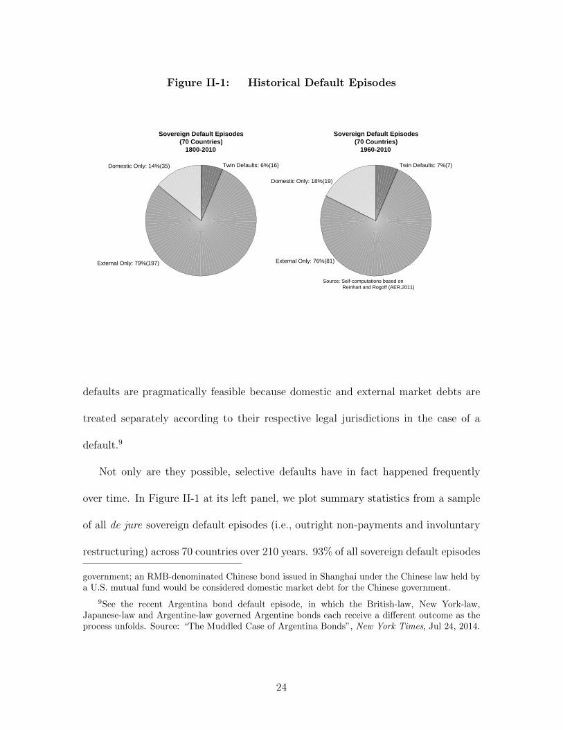
Figure II-1: Historical Default Episodes

Sovereign Default Episodes(70 Countries)

1800-2010

Domestic Only: 14%(35)

External Only: 79%(197)

Twin Defaults: 6%(16)

Sovereign Default Episodes(70 Countries)

1960-2010

Domestic Only: 18%(19)

External Only: 76%(81)

Twin Defaults: 7%(7)

Source: Self-computations based on Reinhart and Rogoff (AER,2011)

defaults are pragmatically feasible because domestic and external market debts are

treated separately according to their respective legal jurisdictions in the case of a

default.9

Not only are they possible, selective defaults have in fact happened frequently

over time. In Figure II-1 at its left panel, we plot summary statistics from a sample

of all de jure sovereign default episodes (i.e., outright non-payments and involuntary

restructuring) across 70 countries over 210 years. 93% of all sovereign default episodes

government; an RMB-denominated Chinese bond issued in Shanghai under the Chinese law held bya U.S. mutual fund would be considered domestic market debt for the Chinese government.

9See the recent Argentina bond default episode, in which the British-law, New York-law,Japanese-law and Argentine-law governed Argentine bonds each receive a different outcome as theprocess unfolds. Source: “The Muddled Case of Argentina Bonds”, New York Times, Jul 24, 2014.

24

in the sample are selective (i.e., 14% of domestic only and 79% of external only).10

Such a high probability is partially driven by improper accounting — we count it as a

selective default when a country explicitly defaults on its external debt and implicitly

defaults on its domestic debt via hyper-inflations. To account for de facto defaults

beyond the de jure ones, we plot these summary statistics again in Appendix A7 with

additional considerations for hyper-inflations. Despite some changes in numbers, the

key idea that selective defaults are frequent phenomena remains compelling across

different specifications.

Furthermore, Figure II-1 also shows that external defaults seem much more likely

than domestic defaults. Over 1800-2010, 85% of the sovereign defaults involve ex-

ternal markets (i.e., 79% of external only and 6% of twin defaults) while only 20%

involve domestic markets (i.e., 14% of domestic only and 6% of twin defaults). To

ensure this is not just driven by a few outlier countries but more of a general phe-

nomenon, we plot similar statistics at the country level in Appendix A8 and conclude

that external defaults are indeed more likely than domestic defaults across countries.

Overall, this suggests that any theory of selective defaults should be able to account

for this phenomenon, and fortunately our model is able to achieve this as well.

10We also plot summary statistics using a sub-sample over 1960-2010 at the right panel in FigureII-1; the message stays strikingly consistent no matter which time frame we look at within thesample.

25

B. A Sovereign Debt Model with Two Markets

In this section we outline a novel general equilibrium sovereign debt model, in which

the benevolent government can strategically choose to borrow from domestic or ex-

ternal markets. We assume that the government borrows from both households and

residing foreigners on its domestic market, whereas it borrows only from non-resident

foreigners on its external market. The government cannot commit to repay its debts

ex-post on both markets per Eaton and Gersovitz (1981), but it can choose to selec-

tively default on either market.

Households solve an inter-temporal consumption problem. Their representative

agent receives a Markov stochastic stream of endowments yt > 0 that follows a tran-

sition function f(yt+1, yt) and has compact support Y . Its objective is to maximize

its expected lifetime utility, and in doing so, it chooses its private goods consumption

ct in each period, taking public goods consumption gt as given.

Formally, households

max{ct}

+∞∑t=0

βtE0 [u (ct, gt)] ,

subject to their inter-temporal budget constraint that takes shape after the govern-

ment makes its borrowing and default decisions each period. β ∈ (0, 1) denotes the

households’ subjective period discount factor. u(ct, gt) denotes the households’ period

utility function. It takes a standard constant relative risk aversion (CRRA) utility

functional form with a constant elasticity of substitution (CES) aggregator

u(Ct) =C1−σt − 1

1− σwith Ct = (scc

ρt + (1− sc)gρt )

1ρ ,

26

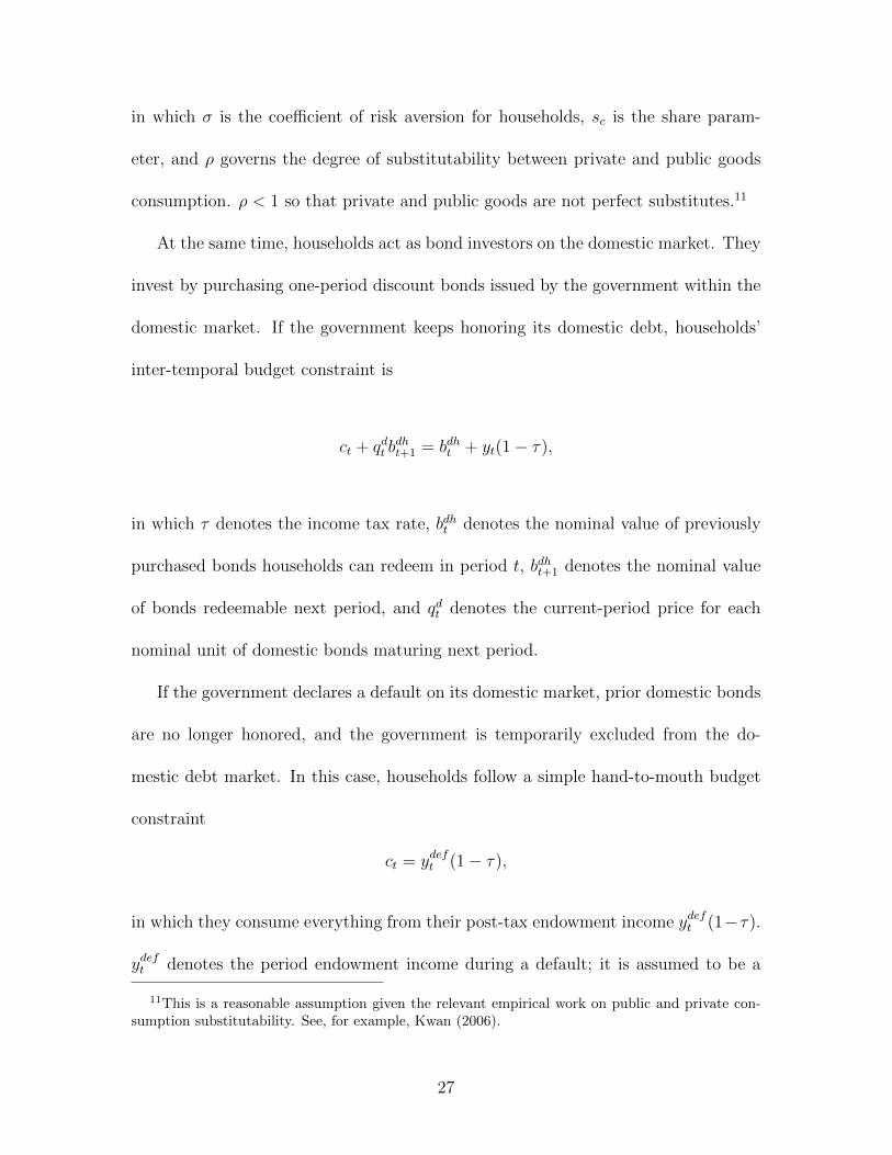
in which σ is the coefficient of risk aversion for households, sc is the share param-

eter, and ρ governs the degree of substitutability between private and public goods

consumption. ρ < 1 so that private and public goods are not perfect substitutes.11

At the same time, households act as bond investors on the domestic market. They

invest by purchasing one-period discount bonds issued by the government within the

domestic market. If the government keeps honoring its domestic debt, households’

inter-temporal budget constraint is

ct + qdt bdht+1 = bdht + yt(1− τ),

in which τ denotes the income tax rate, bdht denotes the nominal value of previously

purchased bonds households can redeem in period t, bdht+1 denotes the nominal value

of bonds redeemable next period, and qdt denotes the current-period price for each

nominal unit of domestic bonds maturing next period.

If the government declares a default on its domestic market, prior domestic bonds

are no longer honored, and the government is temporarily excluded from the do-

mestic debt market. In this case, households follow a simple hand-to-mouth budget

constraint

ct = ydeft (1− τ),

in which they consume everything from their post-tax endowment income ydeft (1−τ).

ydeft denotes the period endowment income during a default; it is assumed to be a

11This is a reasonable assumption given the relevant empirical work on public and private con-sumption substitutability. See, for example, Kwan (2006).

27

depressed level of yt, depending on the exact default status on the two markets.

Foreign investors reside on both domestic and external markets so they invest

on both domestic and external bonds. However, they are subject to a capital control

constraint on the domestic market: only a limited entry of foreign investments is

allowed into the domestic domain. Formally,

bdft+1 ≤ γbdht+1,∀t,

in which bdft+1 denotes the nominal value of domestic bonds purchased by foreign

investors in period t, and γ ∈ [0,+∞) governs the degree of domestic capital controls.

If γ = 0, the domestic market is completely shut off to foreign investors; if γ = +∞,

the domestic market imposes no constraints over foreign investors.

Foreign investors are risk-neutral, and they are willing to borrow or lend as much

as they need to, as long as they are compensated with an expected return of the

constant international risk-free lending rate rf > 0.

With perfect information on the debtor country income process, foreign investors

price the defaultable bonds in a risk-neutral manner so that they break even in

expected value in every bond contract. However, since domestic and external bonds

have different default probabilities, this requires domestic bond prices qdt and external

bond prices qet to separately satisfy

qdt =1− δdt+1

1 + rf; qet =

1− δet+1

1 + rf.

28

in which δdt+1, δet+1 respectively denote the expected probabilities of debtor country

default in period t+ 1 on domestic and external markets.

The next-period default risks δdt+1, δet+1 are endogenous to the model. They depend

on the government’s incentives to default domestically or externally under different

possible yt+1 realizations. In equilibrium, they are sums of probabilities for yt+1

realizations in the next period, in which the government finds it optimal to default

on the respective market. Formally,

δdt+1 =

∫DD(bdht+1,b

dft+1,B

et+1)

f(yt+1, yt)dyt+1; δet+1 =

∫ED(bdht+1,b

dft+1,B

et+1)

f(yt+1, yt)dyt+1,

in whichDD(bdht+1, bdft+1, B

et+1) ≡ {yt+1 ∈ Y : government chooses a domestic default},

and ED(bdht+1, bdft+1, B

et+1) ≡ {yt+1 ∈ Y : government chooses an external default}.12

The benevolent government solves a strategic borrowing and default problem

in this economy. Entering each period, it receives its current-period tax income τyt,

provides public goods consumption gt for households, and decides whether to repay

on its maturing domestic and external debts (bdht , bdft , B

et ). If it does, it continues to

borrow by selling bonds with face values (bdht+1, bdft+1, B

et+1) at unit prices of (qdt , q

et ).

If not, it declares a default on its domestic debt, or its external debt, or both. Ma-

turing debts within the markets in default are ignored, but no new bonds could be

issued in the respective markets. The general inter-temporal budget constraint for

the government is τyt + qdt (bdht+1 + bdft+1) + qetB

et+1 = bdht + bdft +Be

t + gt.

Defaulting on either market has two consequences — temporary financial exclusion

12A formal introduction of DD(bdht+1, bdft+1, B

et+1) and ED(bdht+1, b

dft+1, B

et+1) are deferred until ex-

positions on the government’s strategic default problem.

29

and direct output loss. The debtor country loses its access to the respective debt

market and only regains access with exogenous probabilities (θd, θe ∈ [0, 1)) during

each subsequent period. For as long as the debtor country is in default of either

market, its output remains at a depressed level ydef . Depressed output level ydeft is

assumed to be a concave piecewise liner function with a kink at a variable threshold

y, depending on specific default status of the debtor country. Formally,

ydeft = min{yt, y},

where

y =

ωey, if external default only

ωdy, if domestic default only

ωeωdy, if twin default

and y denotes the long-run average of yt.

Formally, the government’s strategic borrowing and default problem is outlined

below. (For brevity of notations, I drop all t-subscripts and replace t+1notations with

’ variables.) Entering each period, the government is maximizing its welfare value

function V o(bdh, bdf , Be, y) by choosing among repaying all debts V r(bdh, bdf , Be, y),

defaulting domestically V d(Be, y), defaulting externally V e(bdh, bdf , y), and defaulting

on both markets V b(y),

V o(bdh, bdf , Be, y) = maxV r,V d,V e,V b

{V r(bdh, bdf , Be, y), V d(Be, y), V e(bdh, bdf , y), V b(y)

}.

30

Specifically, the value function of repaying all debts V r(bdh, bdf , Be, y) is

V r(bdh, bdf , Be, y) = maxbdh′ ,bdf ′ ,Be′

{u(C) + β

∫y′V o(bdh

′, bdf

′, Be′ , y′)f(y′, y)dy′

}.

The value function of being in domestic default V d(Be, y) is

V d(Be, y) = maxBe′

{u(C) + β

∫y′

[θdV o(0, 0, Be′ , y′)

+(1− θd) maxV d,V b

{V d(Be′ , y′), V b(y′)

}]f(y′, y)dy′

}.

The value function of being in external default V e(bdh, bdf , y) is

V e(bdh, bdf , y) = maxbdh′ ,bdf ′

{u(C) + β

∫y′

[θeV o(bdh

′, bdf

′, 0, y′)

+(1− θe) maxV e,V b

{V e(bdh

′, bdf

′, y′), V b(y′)

}]f(y′, y)dy′

}.

The value function of being in default on both markets V b(y) is

V b(y) = u(C) + β

∫y′

[θdθeV o(0, 0, 0, y′) + θd(1− θe)V e(0, 0, y′)

+(1− θd)θeV d(0, y′) + (1− θd)(1− θe)V b(y′)]f(y′, y)dy′.

The choices among V r, V d, V e, V b constitute the government’s default policy sets

for the domestic market (DD(bdh, bdf , Be)) and the external market (ED(bdh, bdf , Be)).

Formally,

DD(bdh, bdf , Be) ≡{y ∈ Y : max{V r, V d, V e, V b} ∈ {V d, V b}

},

31

and

ED(bdh, bdf , Be) ≡{y ∈ Y : max{V r, V d, V e, V b} ∈ {V e, V b}

}.

With the households, the foreign investors, and the government in place, we now

define the recursive equilibrium in this economy.

Definition. The recursive equilibrium in this economy is formally defined as the

policy functions/sets {ct}+∞0 , {gt}+∞

0 , DD(bdh, bdf , Be), ED(bdh, bdf , Be), {bdht+1}+∞0 ,

{bdft+1}+∞0 , {Be

t+1}+∞0 , and market prices {qdt }+∞

0 , {qet }+∞0 such that

1. households maximize their expected lifetime utility subject to their budget con-

straint, taking as given the government default policies and public goods provi-

sions;

2. the government default policies and borrowing choices satisfy its optimization

problem, taking as given the endogenous prices for both domestic and external

bonds issued;

3. endogenous bond prices reflect corresponding default probabilities in respective

market, and are consistent with foreign investors’ expected zero profits condition;

4. domestic market bond holdings between households and residing foreigners sat-

isfy the capital control constraint,

taking as given the stochastic endowment process {yt}+∞0 .

To demonstrate how a home bias of sovereign borrowing can arise as an equilibrium

outcome in the model, we computationally solve for equilibrium solutions using a

32

counterfactual calibration. The goal of this calibration is not to match to any specific

economy; instead, it is meant to show how the “home bias” of sovereign borrowing

can occur in such a model under reasonable assumptions and calibrations to that of

a “typical” emerging market economy.

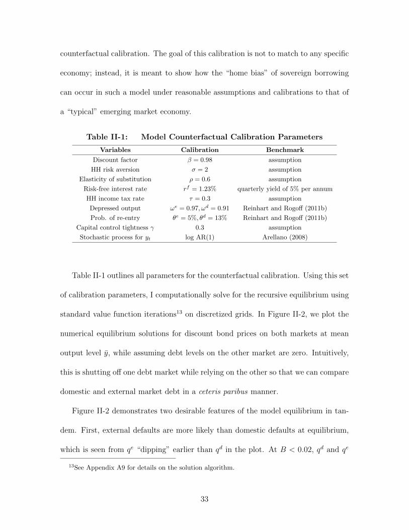
Table II-1: Model Counterfactual Calibration Parameters

Variables Calibration Benchmark

Discount factor β = 0.98 assumption

HH risk aversion σ = 2 assumption

Elasticity of substitution ρ = 0.6 assumption

Risk-free interest rate rf = 1.23% quarterly yield of 5% per annum

HH income tax rate τ = 0.3 assumption

Depressed output ωe = 0.97, ωd = 0.91 Reinhart and Rogoff (2011b)

Prob. of re-entry θe = 5%, θd = 13% Reinhart and Rogoff (2011b)

Capital control tightness γ 0.3 assumption

Stochastic process for yt log AR(1) Arellano (2008)

Table II-1 outlines all parameters for the counterfactual calibration. Using this set

of calibration parameters, I computationally solve for the recursive equilibrium using

standard value function iterations13 on discretized grids. In Figure II-2, we plot the

numerical equilibrium solutions for discount bond prices on both markets at mean

output level y, while assuming debt levels on the other market are zero. Intuitively,

this is shutting off one debt market while relying on the other so that we can compare

domestic and external market debt in a ceteris paribus manner.

Figure II-2 demonstrates two desirable features of the model equilibrium in tan-

dem. First, external defaults are more likely than domestic defaults at equilibrium,

which is seen from qe “dipping” earlier than qd in the plot. At B < 0.02, qd and qe

13See Appendix A9 for details on the solution algorithm.

33

Figure II-2: Equilibrium Bond Prices qd, qe at Mean Output y

(Solid Line — qe, Dashed Line — qd)

0 0.02 0.04 0.06 0.08 0.1 0.12 0.14 0.16B

0

0.1

0.2

0.3

0.4

0.5

0.6

0.7

0.8

0.9

q

Equilibrium Discount Rates of Sovereign Bonds at Mean Output(Domestic Market Only qd vs. International Market Only qf)

qf

qd

both plateau at 11+rf

since there is no perceivable default risk yet on both markets

at such low levels of debt. However, at 0.02 < B < 0.028, more debt is borrowed on

both markets, and qe tanks to reflect the increased default risk while qd still plateaus

at 11+rf

. In fact, at any point within 0.02 < B < 0.045, external default risk is always

higher than domestic default risk for a given debt level. This corresponds well with

earlier empirical observation in that external defaults are historically more likely than

domestic defaults for a given country.

Second, domestic debt is always cheaper — if not equal — to borrow than external

34

debt when borrowing an identical amount of debt on either market. At all debt levels

in the plot, qe has always been beneath — if not equal to — qd, and this means the

cost of borrowing for a given amount of debt is lower on the domestic market than

the external market, ceteris paribus. As the government prioritizes domestic debt to

lower its costs of financing, the model generates the observed “home bias” in sovereign

borrowing.

C. Relationship between Capital Control

Measures and Home Bias of Sovereign

Borrowing

The model implies a relationship between a country’s capital control measures and its

home bias of sovereign borrowing through the constraint bdft+1 ≤ γbdht+1. In the model,

a higher γ allows more foreign capital bdft+1 on the domestic market, and hence the

government has less need to supplement its hedging needs with external debt. As a

result, the degree of home bias in sovereign borrowing is stronger. But empirically,

is this borne out in the data?

To test out this relationship in the data, we compile a cross-country dataset that

spans 58 countries over 1996-2010 and run a multivariate cross-sectional regression

using long-run averages.14 We formally specify the regression below, and summarize

14Alternatively we could have run a panel regression using this dataset. However, it would largelybe the same as a cross-sectional regression using long-run averages. This is because capital controlmeasures are rarely changing over years for most countries and the panel regression would have

35

its full results in Table II-2. As a quick preview, these results show that looser inflow

capital control measures on the domestic market are indeed associated with a stronger

home bias in the sovereign borrowing of a country.

Specification (Multivariate Cross-country Test using Long-run Averages).

dSharei = β0 + βcnetInflowi + Xi + µi,

in which i denotes a country, dSharei measures its degree of home bias in sovereign

borrowing, netInflowi measures its degree of financial openness to net capital inflows

on the domestic market, and Xi denotes all other controls including the rule of law

index, the total sovereign debt to GDP ratio, the real gross domestic product, the real

GDP per capita, the gross savings to GDP ratio, the annualized inflation rate, the

current account balance to GDP ratio and the annualized average GDP growth.

We construct the degree of home bias dSharei using the sample average of annual

domestic/total debt shares for country i over 1996-2010, adjusted into a common

currency of US dollars. Formally,

dSharei =1

T

T∑t

country i’s outstanding domestic debt in $ at year t

country i’s outstanding total debt in $ at year t.

To construct these domestic debt shares, we use data from Reinhart and Rogoff

(2011a), cross checked and supplemented with data from Cowan et al (2006), Guscina

and Jeanne (2006), and Panizza (2008).

almost no intra-country inter-temporal variations in its independent variable.

36

Table II-2: Regressions of Domestic Debt Shares on netInflow Openness

Variables domestic Debt/total Debt

netInflow 0.052(0.024)

** 0.058(0.021)

*** 0.059(0.029)

** 0.061(0.028)

**

Rule Of Law 0.164(0.044)

*** 0.208(0.017)

***

Constant 0.215(0.169)

0.403(0.068)

*** −0.032(0.166)

−0.029(0.165)

Macro Controls All Selected All Selected

total Debt/GDP 0.095(0.068)

0.125(0.071)

* 0.133(0.065)

**

GDP 12.493(9.200)

2.496(8.352)

GDP/capita 1.359(2.350)

9.244(1.442)

*** 9.566(1.360)

***

gross savings/GDP 1.321(0.616)

** 0.606(0.231)

** 2.297(0.646)

*** 2.126(0.649)

***

inflation −0.516(0.536)

−1.397(0.618)

** −1.038(0.323)

***

current account/GDP −1.334(0.931)

−3.102(0.871)

*** −2.956(0.866)

***

GDP growth −0.303(0.778)

−0.628(0.958)

n 56 58 56 56

R2 0.727 0.691 0.647 0.644

F 24.11 62.27 19.16 25.47

Prob. > F 0.000 0.000 0.000 0.000

Notes: All ratios (including inflation and GDP growth) are in decimals. All variables for each countryare inter-temporal averages over 1996-2010, in which inflation, GDP growth are computed using annualizedaverages while the rest are simple arithmetic means. All GDP data are deflated to 2010 US$, in which GDPare in quadrillions US$ while GDP/capita are in millions US$.Robust standard errors are reported in parentheses below the coefficient estimates; * is significant at 10%,** is significant at 5% and *** is significant at 1%.

We construct the financial openness index netInflowi using more primitive re-

striction indices developed by FKRSU-2016 (Fernandez, Klein, Rebucci, Schindler

& Uribe, 2016).15 To develop quantitative measures on capital control policies, they

encode textual policy descriptions from IMF AREAER reports16 into numeric indices

15This paper has a few earlier editions in the same spirit including Schindler (2009), Klein (2012),and Fernandez, Klein & Uribe (2015).

16IMF AREAER (i.e., International Monetary Fund Annual Report on Exchange Arrangementsand Exchange Restrictions) reports are frequently used as primary sources of capital control policies

37

∈ [0, 1] that measure capital control restriction intensities on both inflows and out-

flows of different cross-border transaction types. To construct netInflowi, we use

average financial openness for capital inflows less average financial openness for capi-

tal outflows, specifically on money market transactions, bond transactions, derivative

investments transactions, and financial credit transactions.17

Formally,

netInflowi =1

T

T∑t

inflowi,t −1

T

T∑t

outflowi,t,

in which i, t denotes a country-year, inflowi,t = 14[(1 −mmii,t) + (1 − boii,t) + (1 −

deii,t)+(1−fcii,t)], outflowi,t = 14[(1−mmoi,t)+(1−booi,t)+(1−deoi,t)+(1−fcoi,t)],

and mmii,t, mmoi,t, boii,t, booi,t, deii,t, deoi,t, fcii,t, fcoi,t are primitive restriction

indices on specific transaction type inflows/outflows taken from FKRSU-2016.18

Among all other controls we include a rule of law index that is taken from the

Worldwide Governance Indicators. It is included to control for heterogeneity in home

bias of sovereign borrowing that arises directly from differences in legal environments

between home and abroad. All macroeconomic controls are constructed using data

from IMF WEO database.19 These are in place to account for cross-country differ-

for developing quantitative measures. Earlier works include Quinn (1997, 2011) and Chinn and Ito(2006, 2008).

17These transaction categories are specifically chosen so that they cover all potential methodsof foreign investments on domestic sovereign bonds. This is because foreign investors residing do-mestically could potentially invest on domestic sovereign bonds through money market instruments,directly on bonds, indirectly through derivatives, or borrowing from banks to invest.

18Specifically, mmii,t, mmoi,t are on money market investment inflows/outflows, boii,t, booi,t areon bond investment inflows/outflows, deii,t, deoi,t are on derivative investment inflows/outflows,and fcii,t, fcoi,t are on financial credit inflows/outflows.

19We use the October 2016 version of IMF WEO database (i.e., International Monetary FundWorld Economic Outlook).

38

ences in macroeconomic conditions.

According to the model, we expect βc in the regression to be positive. Table

II-2 display βc estimates in bold at the first row from the top, and they are indeed

positive and statistically significant. Across different columns in Table II-2, we also

run slightly different specifications of the baseline regression. This is to sanity-check

on robustness of the regression results conditioning on including different controls in

the regressions. Overall, the relationship that looser inflow capital control measures

are associated with stronger home biases remains present and statistically significant

across different specifications.

D. Summary

This chapter sets out with the goal of incorporating domestic debt into sovereign

finance theories. In doing so, it proposes a novel general equilibrium sovereign debt

model, in which the benevolent government can strategically choose to borrow from

the domestic or external markets. Under reasonable assumptions and calibrations,

the observed home bias of sovereign borrowing naturally emerges in the model as

an equilibrium outcome through the government’s strategic financing behaviors. Fi-

nally, this chapter also presents some cross-country evidence for the model-implied

relationship that looser inflow capital control measures for a country are associated

with a stronger home bias in its sovereign borrowing.

39

Chapter III.

The Financial Channel of

Economic Agglomeration

Economic activities tend to agglomerate in space.1 For instance, nearly a third of all

U.S. economic activities take place within merely 1% of total land area in the coun-

try.2 How does economic agglomeration arise in those areas?3 An understanding of

underlying economic forces is crucial because it can guide developments and growths

elsewhere.

1We map economic activities using locations of firms/establishments as in Ellison, Glaeser, andKerr (2010). Others, such as Davis and Weinstein (2002) and Gabaix et al. (2011), have used thespatial distribution of the population.

2The 100 densest counties by the number of establishments per unit land area accounts for 32%of all establishments in the U.S. economy and 1% of total land area in the country. The U.S. CensusBureau defines an establishment as “a single physical location where business is conducted or whereservices or industrial operations are performed.” See Appendix A10 for a map of U.S. economicdensity at the county-level.

3While natural advantages and random chances partly contribute to the economic prosperity inthose areas, they hardly represent the whole story (Ellison and Glaeser, 1997, 1999; Duranton andOveman, 2005). In this case, “natural advantages” are defined broadly as in Ellison and Glaeser(1999). One example is the relatively low electricity prices in Washington as a “natural advantage”for economic productions.

40

Traditionally, urban economists interpret economic agglomeration as an outcome

of firms choosing to locate near each other, because doing so begets increasing returns

to scale in their productions.4 To explain economic agglomeration, these theories

show that firms would endogenously choose to move near each other in a spatial

equilibrium, when production factors (especially labor) are perfectly mobile (Glaeser

and Gottlieb, 2009). However, sometimes moving costs, in reality, are likely so large

that any mobility becomes impossible to achieve.5

Alternatively, chapter 3 explores the possibility of explaining economic agglom-

eration from a novel financial perspective — the financial channel of economic ag-

glomeration. The basic idea posits that firms would more likely emerge together

near banks due to less stringent financial frictions in obtaining bank loans, and firms

subsequently agglomerate in these areas as they grow over time.6

4Such increasing returns could come from savings in trade costs (e.g., Krugman, 1991b; Allen andArkolakis, 2014), labor-market pooling (e.g., Krugman 1991a; Strange et al., 2006), or knowledgespillovers (e.g., Duranton and Puga, 2001; Davis and Dingles, 2019). The original ideas of savings intrade costs, labor-market pooling, and knowledge spillovers all date back to Marshall (1890, 1920),and all three theories have considerable empirical support (Ellison, Glaeser and Kerr, 2010). Otherimportant earlier works about savings in trade costs include Fujita, Krugman and Venables (1999);works about labor-market pooling include Diamond and Simon (1990), Helsley and Strange (1990),Costa and Kahn (2000), Fallick, Fleischman and Rebitzer (2006), Freedman (2008); works aboutknowledge spillovers include Glaeser et al (1992), Audretsch and Feldman (1996), Glaeser and Mare(2001), Lucas (2001), Berliant, Peng and Wang (2002), Henderson (2003), Helsley and Strange(2004), Moretti (2004), Berliant, Reed III and Wang (2006), and Freedman (2008). See Glaeser andGottlieb (2009) for a quick tour of the intellectual lineage, and Duranton and Puga (2004), Moretti(2011) for more surveys of the related literature.

5Rauch (1993) has theoretically demonstrated how strategic complementarity could create a first-mover disadvantage that prevents any relocation of firms. A recent strand of empirical literature(Bryan, Chowdhury and Mobarak, 2014; Chetty, Hendren and Katz, 2016; Munshi and Rosen-zweig, 2016; Nakamura and Steinsson, 2018; Bryan and Morten, forthcoming) looks at economicconsequences of moving for people and concludes that moving costs — arising from informational,cultural, legal, and economic barriers — of labor must be so substantial that people are often “stuck”in locations that do not fully realize their economic potentials.

6Duranton and Kerr (2015) are the first to discuss financial frictions being potentially importantfor understanding economic agglomeration.

41

Such a channel is theoretically feasible, given what we have learned from existing

research. First, firms could indeed more likely emerge due to less stringent finan-

cial frictions because entrepreneurship requires external financing, and the ability to

borrow is vital for firm formations (Evans and Jovanovic, 1989). Second, financial

frictions could be less stringent near banks because a shorter borrower-lender distance

does improve lending terms in bank loans (Mian, 2006; Bolton et al, 2016).7 And

third, frictions in obtaining bank loans could really matter because the average U.S.

firm heavily relies on bank loans for external financing (Peterson and Rajan, 2002).

However, whether such a channel exists in the data is a difficult empirical question.

Merely observing more firms locate near banks in the cross-section8 is insufficient for

at least two reasons. First, there could be omitted variable biases in that firms and

banks can collocate for reasons unrelated to borrowing and lending (Fujita and Mori,

1996; Ellison and Glaeser, 1999; Davis and Weinstein, 2002).9 Second, there could

be reverse causality in that banks posteriorly locate themselves in places where firms

already agglomerate.10

To show that a bank can indeed cause firms to agglomerate in its proximity by

easing their financial frictions, chapter 3 designs a natural experiment by exploiting

7The distance effects could come from a variety of microeconomic mechanisms, such as lesscostly monitoring (Rajan, 1992; Von Thadden, 1995), better information acquisition (Agarwal andHauswald, 2010; Puri et al., 2010), and less severe principal-agent problem (Stein, 2002).

8See Appendix A10 for a cross-sectional plot observing more firms locate near banks.

9Historical narratives have also emphasized the importance of inherent natural advantages inthe rise of well-known metropolises such as New York City, Chicago, and Pittsburgh. See Albion(1938) and Cronon (1991) for more details.

10Anecdotal evidence suggests that banks indeed relocate themselves to “chase the crowd.”See, for example, “Bank of Commerce Holdings Announces Relocation of Headquarters” (GlobeNewswire, 2017a) and “First U.S. Bancshares, Inc. Announces Relocation of Headquarters to Birm-ingham” (Globe Newswire, 2017b).

42

the sudden location change on the target bank after each banking merger — in that

the target bank suddenly “relocates” (through merging) to the acquiring bank. The

intuition is to see what a quasi-exogenous relocation of a bank closer to a region does

to the region’s total loan supplies and subsequent establishment growths. A standard

difference-in-difference (Diff-in-Diff) approach shows that relocation of a bank closer

to a region indeed causes more supply of bank loans in that region, and subsequently

causes more firm establishments to emerge and agglomerate within the same area.11

Two major identifying assumptions have to hold for this strategy to be successful.

First, absent the treatment, outcomes at the “treated” regions would evolve similarly

as those of the “control” regions, and one necessary condition for this assumption to

hold is the so-called “parallel pre-trend” — trends in outcome variables between the

two groups are parallel at least before the treatment. We can validate this condition

using our data. Second, no other shocks are happening at the same time of treatment

that could potentially affect the outcome variables. To alleviate this concern, we

include additional controls to proxy for such shocks in our regression specifications.

This chapter organizes itself as follows. Section A discusses the identification

strategy in detail. Section B briefly outlines the data sources we use as well as the

sample construction process. Section C formally spells out the Diff-in-Diff specifica-

tion. Section D validates the parallel pre-trend condition. Section E presents the full

set of regression results. Finally, section F concludes the chapter.

11Guiso, Sapienza, and Zingales (2004) study how having nearby banks could help local economicgrowth through promoting entrepreneurship in Italy. In some way, this chapter studies an analog ofthat question in the context of the U.S.

43

A. Identification Strategy

To identify if a bank can indeed cause firms to agglomerate within its proximity by

easing their financial frictions in obtaining loans, we design a natural experiment

that resembles a hypothetical randomized controlled trial. In such a trial, we would

first want to exogenously move a bank closer to or away from its lending areas while

controlling for other factors, and then examine consequences on total loan supplies

and subsequent firm/establishment growths within the same areas.

Correspondingly, the natural experiment generates a quasi-exogenous bank relo-

cation, by exploiting the sudden location change of the target bank after a banking

merger. As the target bank suddenly “relocates” (through merging) to the acquiring

bank, we examine loan and firm/establishment outcome changes within the target

bank lending areas, which can become closer to or farther away from the bank after

the merger. To maximally control for other factors during this process, we develop a

procedure that carefully isolates the “relocation shock” from other things happening

at the same time as the merger. To do so, we proceed in three steps.

First, we compile a list of large-scale banking mergers over 1998-2015 as events

generating the relocation shocks, in which each merger gives us one natural experi-

ment.12 In this case, large-scale banking mergers are those with individual pre-merger

total assets above $1 billion from both merging banks. We only look at these merg-

ers to reduce concerns of reverse causality — since it is unlikely that local loan and

firm/establishment outcome changes are driving merger decisions in deals of such

12We perform repeated natural experiments using a pooled sample, as in Greenstone, Hornbeck,and Moretti (2010).

44

sizes. This tactic has been used by Nguyen (2019) to alleviate reverse causality con-

cerns.

Second, we sample all de novo counties associated with each merger and use each

county as a controlled environment, in which we later examine outcomes of different

ZIP-code areas. We define de novo counties as counties in which only the target

bank (out of the merging banks) had full-service deposit-taking branches before the

merger.13 In these counties, the merger does not create market structure changes

in the local banking markets.14 Furthermore, regulations keep existing target bank

branches intact after the merger. These features help us maximally control for other

things happening at the same time as the merger within the natural experiment.15

Finally, within each de novo county from the sample, we examine total bank loan

originations and firm/establishment growths across different ZIP-code areas. We use

a Census-defined ZIP Code Tabulation Area (ZCTA) as a unit of observation for

ZIP-code areas,16 and we coarsely define a ZCTA as a lending area for a bank if

the bank has full-service deposit-taking branches within the ZCTA. Following these

definitions, we consider the target bank lending ZCTAs within each de novo county

13We name these counties as “de novo” from the perspective of the acquirer because it is througha particular merger the acquiring bank first enters these counties. In Appendix A11, we illustratethe concept of de novo counties using an example.

14In local banking markets within these counties, no consolidation occurs as the acquiring banktakes the place of the target bank after the merger. In other counties where both the target and theacquiring banks were present before the merger, consolidation occurs, and the acquiring bank has amuch higher market power after the merger.

15U.S. regulations require that all merging banks commit to maintain existing services at com-munities which the non-surviving bank has previously provided. In de novo counties, the acquiringbank typically maintains the target bank’s existing branches together with all their prior servicesand local banking relationships. In other counties, branch closures frequently occur after the mergerif the acquiring bank already has incumbent branches before the merger.

16A ZIP Code Tabulation Area (ZCTA) is a collection of contiguous Census blocks that consoli-date nearby areas of similar ZIP codes.

45

as the “treated” areas and all other ZCTAs as the “control” areas in the natural

experiment.

Using a standard difference-in-difference (Diff-in-Diff) approach to compare out-

comes across “treated” and “control” ZCTAs before and after each merger, we can

then identify if a quasi-exogenous relocation of a bank indeed affects total loan sup-

plies and firm/establishment growths within its lending area. We use strong fixed

effects to ensure we only compare across ZCTAs within each de novo county from a

particular merger. We discuss the formal regression specification in a later section.

B. Data Sources and Sample Construction

To carry out the identification strategy outlined above, we need several sources of

information on the U.S., including data on banking mergers, data on bank branch

spatial networks, disaggregate data on total bank loan originations by region, and

disaggregate data on establishment growths by region.

Information on U.S. banking mergers is available from the Mergers and Acquisi-

tions dataset by the Federal Reserve Bank of Chicago (FRB Chicago) through the

National Information Center (NIC). Per U.S. banking regulations, all mergers have

to be reported to and approved by the Federal Reserve System. As such, this dataset

contains information “that can be used to identify all bank and bank holding com-

pany (BHC) acquisitions and mergers that have occurred since 1976” (FRB Chicago).

Merging it with the standard Call Reports at the bank-level, we can then shortlist all

U.S. banking mergers from 1998 - 2015 that have pre-merger individual total assets

46

above $1 billion. We start from 1998 in our sample because the Riegle-Neal Act that

enables complete inter-state banking mergers only went into effect in June 1997.

Geospatial information on bank-branch networks comes from the Summary of De-

posits (SOD) dataset compiled by the Federal Deposit Insurance Corporation (FDIC).

The SOD is, per the FDIC websites, “[a required] annual survey of branch office de-

posits as of June 30 for all FDIC-insured institutions, including insured U.S. branches

of foreign banks.” In other words, we can use it to locate all full-service deposit-taking

branches of any commercial bank to the ZIP-code level. This information is crucial

for sampling de novo counties as well as designating “treated” and “control” ZCTAs

within each county.

Disaggregate data on total bank loan originations by region are available at the

Federal Financial Institutions Examination Council (FFIEC) through the Community

Reinvestment Act (CRA) enacted in 1977. Per CRA regulatory requirements, all U.S.

commercial banks above a threshold in total assets are required to report their annual

business loan originations to FFIEC for compliance assessments.17 Aggregating this

information across banks, the FFIEC creates a dataset at the Census-tract level, and

it contains annual total bank loan originations (in both quantities and dollar amounts)

to all firms having less than $1 million annual revenues within a Census-tract.

Disaggregate data on establishment growths by region are from the County Busi-

ness Patterns (CBP) dataset developed from the Longitudinal Business Data (LBD)

database by the U.S. Census Bureau. It contains establishment-level information on

17This threshold is approximately $1 billion and it is slightly adjusted every year to account forgeneral inflations. In 2010, “the asset size threshold that triggers data collection and reporting forall agencies is $1.098 billion as of December 31 of each of the prior two calendar years” (FFIEC).

47

employment counts, payroll amounts, industry classification, and ZIP codes.

In our regression specification, we also include other controls on natural geogra-

phies (i.e., local weather and land cover information) and demographic characteristics

(i.e., population size, urban ratio, household income level, labor force participation

ratio, and housing vacancy ratio). These controls are in place so that we can elimi-

nate regional heterogeneities in total bank loan supplies and subsequent establishment

growths that are coming from natural advantages.

Data on natural geographies are from the National Land Cover Database (NLCD)

and the PRISM Climate Database (PRISM CD). The NLCD provides a Census-tract

level land area together with a characterizing vector of proportions for different land

cover types (e.g., open water and grassland) once every five years (i.e., 2001, 2006,

and 2011). The PRISM CD provides a county-level mean and standard deviation of

year-round precipitations and temperatures once every year. Data on demographic

characteristics are from the decennial U.S. Census of 1990, 2000, and 2010, and they

contain information on essential demographics at the ZIP-code level.

While merging different datasets outlined above, we have to deal with different

geographic units and time frequencies frequently. We use the 2010 Reference Files

published by the U.S. Census Bureau to map across different geographic units (e.g.,

from Census-tracts to ZCTAs, and vice versa). To match across different time fre-

quencies (e.g., matching decennial Census data to annual establishment counts data),

we use the last updated observation from datasets with lower time frequencies to fill

gaps in datasets with higher time frequencies until the next available value — for

example, we use 2000 Census observation for 2000-2009 and use 2010 Census obser-

48

vation for 2010 and above in our constructed sample.

Table III-1: Sample Summary Statistics

No. of States 43

No. of Counties 842

%. of Treated ZCTAs 22.7%

No. of Mergers 84

No. of ZCTA-Year Observations 17,597

Upon merging different datasets, we obtain a pooled cross-sectional sample of de

novo counties together with their respective “treated” and “control” ZCTAs from

1998-2015. Table III-1 presents the sample summary statistics. The sample seems

reasonably representative of the U.S. economic landscape as it spans a wide range of

geographic locations in the country.

C. Diff-in-Diff Regression Specification

We employ a continuous treatment Diff-in-Diff regression specification using the “re-

location distance” (∆distancei) as the treatment intensity for a “treated” ZCTA i.

Formally,

∆distancei = distance(ZCTA i, acquiring bank)

− distance(ZCTA i, target bank),

in which distance(A,B) denotes the great-circle distance between locations of A and

B. Intuitively, ∆distancei > 0 means the target bank has “relocated” farther away

49

from its lending ZCTA i after the merger. For “control” ZCTAs within each de novo

county, ∆distancei ≡ 0.

Also, we include a “size shock” (∆sizei) as an additional control in the speci-

fication, because the target bank has not only “relocated” but also become much

bigger in size due to the merger. Intuitively, this is to control for any “size” effects

on lending that are not directly coming from ∆distancei. Formally, ∆sizei denotes

the increase in total assets on the target bank associated with the “treated” ZCTA

i. Again, for “control” ZCTAs, ∆sizei ≡ 0.

We run regressions of total bank loan originations (in $) and log(establishment

counts) in turn using the following specification. Formally,

yi,t = π0 + π1 · Postt + π2 ·∆distancei

+ β ·∆distancei × Postt + π3 ·∆sizei + π4 ·∆sizei × Postt

+ Πc ×Xi,t + Γ + ei,t,

in which yi,t denotes the outcome variables of interest, Postt denotes a dummy vari-

able that equals 1 if the observation is post-merger and 0 if it is pre-merger, Xi,t

denotes controls on natural geographies and demographic characteristics, and Γ de-

notes Merger × County fixed effects. The key coefficient of interest is β. In light

of the financial channel of economic agglomeration, we expect its estimate to be

negative.

In this specification, Xi,t and Γ tremendously alleviate concerns from other fac-

tors that could potentially bias our estimates of β. Xi,t include both natural ge-

50

ographies (i.e., total land area, land cover types, mean and standard deviation of

year-round temperatures and precipitations) and demographic characteristics (i.e.,

ln(population), urban ratio, household income levels, labor force ratio, and housing

vacancy ratio). In addition, the fixed effects Γ can soak up all unobserved hetero-

geneities across different merger-county pairs. Intuitively, this means the variation

this regression uses only comes from within-merger within-county comparisons across

differentially affected ZCTAs.

D. Identifying Assumption — The Parallel

Pre-trend

We check if the “parallel pre-trend” condition holds in our sample using two ap-

proaches. In the first approach, we perform a visual check by plotting simple cross-

sectional averages of total bank loan originations and establishment count growths

over time between the “control” group and the “treated” group with ∆distancei >

0.18 In the second approach, we run a lead-lag version of the discrete treatment Diff-

in-Diff regression using all observations with ∆distancei > 0 as the treated group,

and then examine coefficient estimates before the lead and lag dummies.

Both approaches require long time series data. Since such data are not available

for the entire sample, we construct a constant sub-sample of observations with at

18Recall that it is possible for the target bank to “relocate” closer to its lending ZCTA, and henceit is possible to have ∆distancei < 0. For the purpose of checking the “parallel pre-trend”, we dropobservations with ∆distancei < 0, and they only represent about 3% of the entire sample.

51

Figure III-1: Parallel Pre-Trend in Bank Loan Originations

-7 -6 -5 -4 -3 -2 -1 0 1 2 30

0.5

1

1.5

2

2.5

$.mm

Pre-Trend Analysis in Loan Originations

(using constant sub-sample with at least 10 years' data)

Treated Tracts

Control Tracts

-7 -6 -5 -4 -3 -2 -1 0 1 2 3

No. of full years since treatment

1

1.2

1.4

1.6

1.8

2

$.mm

Treated Tracts

Control Tracts (Shifted)

-7 -6 -5 -4 -3 -2 -1 0 1 2 30

0.5

1

1.5

2

2.5

$.mm

Lead & Lag Diff-in-Diff in Loan Originations

Treated Tracts

Control Tracts

-7 -6 -5 -4 -3 -2 -1 0 1 2 3

No. of years since treatment

-0.4

-0.2

0

t

52

Figure III-2: Parallel Pre-Trend in Establishment Count Growth

-7 -6 -5 -4 -3 -2 -1 0 1 2 30

200

400

600

Nest

Pre-Trend Analysis in Establishments' Growth

(using constant sub-sample with at least 10 years' data)

Treated ZCTAs

Control ZCTAs

-7 -6 -5 -4 -3 -2 -1 0 1 2 3

No. of full years since treatment

0.95

1

1.05

nest

Treated ZCTAs (Normed)

Control ZCTAs (Normed)

-7 -6 -5 -4 -3 -2 -1 0 1 2 30

200

400

600

Nest

Lead & Lag Diff-in-Diff in Establishments' Growth

Treated ZCTA10

Control ZCTA10

-7 -6 -5 -4 -3 -2 -1 0 1 2 3

No. of years since treatment

-0.06

-0.04

-0.02

0

0.02

t

53

least 10 years of data (i.e., 7 years before the merger and 3 years after the merger).

Using the constant sub-sample, we perform the parallel pre-trend analyses using the

two approaches outlined above.

We plot the analysis results for total bank loan originations and establishment

count growths in Figure III-1 and III-2. In top panels of the figures, we do the visual

check of group averages by normalizing the “control” to match against the “treated”

as a counterfactual benchmark of comparison. There is a clear parallel pre-trend

between “treated” and “control” groups before the treatment year, which is defined

as t = 0. In bottom panels of the two figures, we present β estimates together with

their 95% confidence interval bands from the lead-lag regressions (using -2 as the base

year). These estimates show that there are no significant differences between the two

groups before treatment, and it is only after t = 0 we then start to see significant

differences between the two groups.

Overall, there is a clear parallel pre-trend in our sample. This tremendously boosts

our confidence in our identified effects being truly causal.

E. Spatial Causal Effects of A Bank Relocation

on Its Lending Regions

We run the Diff-in-Diff regressions on both total bank loan originations (in $) and

log(estabablishment counts) in turn. Table III-2 and III-3 summarize the results

below.

54

Table III-2: Diff-in-Diff Regression Results on Loan Originations

(1) (2) (3)Loans (in $M) Loans (in $M) Loans (in $M)

Post x ∆ distance -0.0328∗∗∗ -0.0328∗∗∗ -0.0483∗∗∗

(0.00462) (0.00465) (0.00431)

Post -0.0604∗ -0.0604∗ -0.163∗∗∗

(0.0327) (0.0329) (0.0362)

∆ distance (in 100 miles) 0.0230∗∗∗ 0.0267∗∗∗ 0.0283∗∗∗

(0.00560) (0.00475) (0.00457)

Post x ∆ size 0.000111 0.000111 0.000430∗∗∗

(0.000101) (0.000101) (0.0000953)

∆ size (in $ billions) 0.000806∗∗∗ 0.000607∗∗∗ 0.000272∗∗∗

(0.000181) (0.000130) (0.000102)

Demographic Controls No No Yes

Weather Controls No No Yes

Land Cover Controls No No Yes

FE: Merger x County No Yes Yes

Adjusted R2 0.017 0.163 0.276N 78,298 78,298 69,928Number of Clusters 797 797 738

Robust standard errors in parentheses are clustered at the county level.∗ p < 0.10, ∗∗ p < 0.05, ∗∗∗ p < 0.01

Estimates for the key coefficient of interest β are tabulated in the first row in both

tables. These estimates are negative and statistically significant at 1% level, even with

robust standard errors clustered at the county level. We run 3 slight variations of

the same regression by including/excluding additional controls and fixed effects, and

document their respective results in columns (1)-(3). Across different columns, the

estimates for β stay largely constant and they always remain statistically significant.

According to column (3) in both tables, after controlling for the “size shock”,

55

Table III-3: Diff-in-Diff Regression Results on Establishment Growth

(1) (2) (3)ln(Est. Counts) ln(Est. Counts) ln(Est. Counts)

Post x ∆ distance -0.00202∗∗∗ -0.00202∗∗∗ -0.00198∗∗∗

(0.000225) (0.000229) (0.000321)

Post 0.00236 0.00236 0.00458∗

(0.00280) (0.00285) (0.00264)

∆ distance (in 100 miles) 0.00101∗∗∗ 0.00101∗∗∗ 0.000973∗∗∗

(0.000112) (0.000114) (0.000161)

Post x ∆ size 0.0000272∗∗∗ 0.0000272∗∗∗ 0.0000195∗∗∗

(0.00000669) (0.00000681) (0.00000736)

∆ size (in $ billions) -0.0000136∗∗∗ -0.0000136∗∗∗ -0.00000990∗∗∗

(0.00000334) (0.00000341) (0.00000371)

Demographic Controls No No Yes

Weather Controls No No Yes

Land Cover Controls No No Yes

FE: Merger x County No Yes Yes

Adjusted R2 0.016 0.163 0.269N 34,652 34,652 14,212Number of Clusters 842 842 697

Robust standard errors in parentheses are clustered at the county level.∗ p < 0.10, ∗∗ p < 0.05, ∗∗∗ p < 0.01

heterogeneities arising from demographic and natural geographic differences, and

merger-county fixed effects, if we hypothetically move a bank away from its lending

ZCTAs, total bank loan originations in these areas decrease by $48,300 on average for

every 100 miles the bank moves. Subsequently, establishment count growths in these

ZCTAs drop by 0.2% on average. Relatively speaking, this is a large drop in growth

rate, given that the average pre-shock annual establishment count growth across all

ZCTAs is only at about 1%.

56

Overall, these regression results support the financial channel of economic agglom-

eration in that firms/establishments could indeed more likely emerge together near

banks due to less stringent financial frictions in obtaining loans. These results also

suggest the importance of credit availabilities for regional economic growths.

F. Summary

This chapter revisits the classic question of how economic agglomeration arises from a

novel financial perspective. It presents evidence that alternatively explains economic

agglomeration as a result of firms more likely emerging together near banks due to

distance-related frictions in obtaining loans. It does so by designing careful natural

experiments that exploit sudden location changes on banks after banking mergers. A

standard difference-in-difference approach shows that a quasi-exogenous relocation of

a bank closer to a region indeed causes more supply of bank loans to the region, and

subsequently causes more firm establishments to emerge and agglomerate within the

same area.

57

Bibliography

Agarwal, Sumit, and Robert Hauswald. 2010. “Distance and private informationin lending.” The Review of Financial Studies, 23(7): 2757–2788.

Albion, Robert G. 1938. Square-Riggers on Schedule: The New York Sailing Pack-ets to England, France, and the Cotton Ports. Archon Books.

Allen, Treb, and Costas Arkolakis. 2014. “Trade and the topography of thespatial economy.” The Quarterly Journal of Economics, 129(3): 1085–1140.

Arellano, Cristina. 2008. “Default risk and income fluctuations in emergingeconomies.” American Economic Review, 98(3): 690–712.

Arellano, Cristina, and Ananth Ramanarayanan. 2012. “Default and the matu-rity structure in sovereign bonds.” Journal of Political Economy, 120(2): 187–232.

Arslanalp, Serkan, and Takahiro Tsuda. 2014a. “Tracking global demand foradvanced economy sovereign debt.” IMF Economic Review, 62(3): 430–464.

Arslanalp, Serkan, and Takahiro Tsuda. 2014b. “Tracking global demand foremerging market sovereign debt.” IMF Working Paper.

Audretsch, David B, and Maryann P Feldman. 1996. “R&D spillovers and thegeography of innovation and production.” American Economic Review, 86(3): 630–640.

Berliant, Marcus, Robert R. Reed III, and Ping Wang. 2006. “Knowledgeexchange, matching, and agglomeration.” Journal of Urban Economics, 60(1): 69–95.

Berliant, Marcus, Shin-Kun Peng, and Ping Wang. 2002. “Production exter-nalities and urban configuration.” Journal of Economic Theory, 104(2): 275–303.

Bolton, Patrick, Xavier Freixas, Leonardo Gambacorta, and Paolo EmilioMistrulli. 2016. “Relationship and transaction lending in a crisis.” The Review ofFinancial Studies, 29(10): 2643–2676.

Broner, Fernando, Alberto Martin, and Jaume Ventura. 2010. “Sovereignrisk and secondary markets.” American Economic Review, 100(4): 1523–55.

58

Broner, Fernando, and Jaume Ventura. 2011. “Globalization and risk sharing.”The Review of Economic Studies, 78(1): 49–82.

Bryan, Gharad, and Melanie Morten. forthcoming. “The aggregate productiv-ity effects of internal migration: Evidence from Indonesia.” Journal of PoliticalEconomy.

Bryan, Gharad, Shyamal Chowdhury, and Ahmed Mushfiq Mobarak. 2014.“Underinvestment in a profitable technology: The case of seasonal migration inBangladesh.” Econometrica, 82(5): 1671–1748.

Buera, Francisco J, Joseph P Kaboski, and Yongseok Shin. 2015. “En-trepreneurship and financial frictions: A macrodevelopment perspective.” AnnualReview of Economics, 7(1): 409–436.

Bulow, Jeremy, and Kenneth Rogoff. 1989. “A constant recontracting model ofsovereign debt.” Journal of Political Economy, 97(1): 155–178.

Cagetti, Marco, and Mariacristina De Nardi. 2006. “Entrepreneurship, fric-tions, and wealth.” Journal of Political Economy, 114(5): 835–870.

Campbell, John Y, and Robert J Shiller. 1991. “Yield spreads and interest ratemovements: A bird’s eye view.” The Review of Economic Studies, 58(3): 495–514.

Cetorelli, Nicola, and Philip E Strahan. 2006. “Finance as a barrier to entry:Bank competition and industry structure in local US markets.” The Journal ofFinance, 61(1): 437–461.

Chatterjee, Satyajit, and Burcu Eyigungor. 2012. “Maturity, indebtedness, anddefault risk.” American Economic Review, 102(6): 2674–99.

Chetty, Raj, Nathaniel Hendren, and Lawrence F Katz. 2016. “The effectsof exposure to better neighborhoods on children: New evidence from the Movingto Opportunity experiment.” American Economic Review, 106(4): 855–902.

Chinn, Menzie D, and Hiro Ito. 2006. “What matters for financial develop-ment? Capital controls, institutions, and interactions.” Journal of DevelopmentEconomics, 81(1): 163–192.

Chinn, Menzie D, and Hiro Ito. 2008. “A new measure of financial openness.”Journal of Comparative Policy Analysis, 10(3): 309–322.

Cochrane, John H, and Monika Piazzesi. 2005. “Bond risk premia.” AmericanEconomic Review, 95(1): 138–160.

Collin-Dufresne, Pierre, and Robert S Goldstein. 2003. “Generalizing theaffine framework to HJM and random field models.” Working Paper.

59

Costa, Dora L, and Matthew E Kahn. 2000. “Power couples: Changes in thelocational choice of the college educated, 1940–1990.” The Quarterly Journal ofEconomics, 115(4): 1287–1315.

Cowan, Kevin, Eduardo Levy Levy-Yeyati, Ugo Panizza, and FedericoSturzenegger. 2006. “Sovereign debt in the Americas: New data and stylizedfacts.” IDB Working Paper.

Cronon, William. 1991. Nature’s Metropolis: Chicago and the Great West. NewYork and London: Norton.

Davis, Donald R, and David E Weinstein. 2002. “Bones, bombs, andbreak points: The geography of economic activity.” American Economic Review,92(5): 1269–1289.

Davis, Donald R, and Jonathan I Dingel. 2019. “A spatial knowledge economy.”American Economic Review, 109(1): 153–70.

Degryse, Hans, and Steven Ongena. 2005. “Distance, lending relationships, andcompetition.” The Journal of Finance, 60(1): 231–266.

Diamond, Charles A, and Curtis J Simon. 1990. “Industrial specialization andthe returns to labor.” Journal of Labor Economics, 8(2): 175–201.

Duffie, Darrell, and Kenneth J Singleton. 1999. “Modeling term structures ofdefaultable bonds.” The Review of Financial Studies, 12(4): 687–720.

Duffie, Darrell, Lasse Heje Pedersen, and Kenneth J Singleton. 2003. “Mod-eling sovereign yield spreads: A case study of Russian debt.” The Journal of Fi-nance, 58(1): 119–159.

Duranton, Gilles, and Diego Puga. 2001. “Nursery cities: Urban diversity,process innovation, and the life cycle of products.” American Economic Review,91(5): 1454–1477.

Duranton, Gilles, and Diego Puga. 2004. “Micro-foundations of urban agglomer-ation economies.” In Handbook of Regional and Urban economics. Vol. 4, 2063–2117.Elsevier.

Duranton, Gilles, and Henry G Overman. 2005. “Testing for localization usingmicro-geographic data.” The Review of Economic Studies, 72(4): 1077–1106.

Duranton, Gilles, and William R Kerr. 2015. “The logic of agglomeration.”Working Paper.

Du, Wenxin, and Jesse Schreger. 2016a. “Local currency sovereign risk.” TheJournal of Finance, 71(3): 1027–1070.

Du, Wenxin, and Jesse Schreger. 2016b. “Sovereign risk, currency risk, andcorporate balance sheets.” Working Paper.

60

Eaton, Jonathan, and Mark Gersovitz. 1981. “Debt with potential repudiation:Theoretical and empirical analysis.” The Review of Economic Studies, 48(2): 289–309.

Eichengreen, Barry. 1991. “Historical research on international lending and debt.”Journal of Economic Perspectives, 5(2): 149–169.

Eichengreen, Barry, and Ricardo Hausmann. 1999. “Exchange rates and finan-cial fragility.” NBER Working Paper.

Eichengreen, Barry, Ricardo Hausmann, and Ugo Panizza. 2002. “Originalsin: The pain, the mystery, and the road to redemption.” IDB Conference Paper.

Eichengreen, Barry, Ricardo Hausmann, and Ugo Panizza. 2003. “Currencymismatches, debt intolerance and original sin: Why they are not the same and whyit matters.” NBER Working Paper.

Ellison, Glenn, and Edward L Glaeser. 1997. “Geographic concentration in USmanufacturing industries: A dartboard approach.” Journal of Political Economy,105(5): 889–927.

Ellison, Glenn, and Edward L Glaeser. 1999. “The geographic concentration ofindustry: Does natural advantage explain agglomeration?” American EconomicReview, 89(2): 311–316.

Ellison, Glenn, Edward L Glaeser, and William R Kerr. 2010. “What causesindustry agglomeration? Evidence from coagglomeration patterns.” American Eco-nomic Review, 100(3): 1195–1213.

Evans, David S, and Boyan Jovanovic. 1989. “An estimated model of en-trepreneurial choice under liquidity constraints.” Journal of Political Economy,97(4): 808–827.

Fallick, Bruce, Charles A Fleischman, and James B Rebitzer. 2006. “Job-hopping in Silicon Valley: Some evidence concerning the microfoundations of ahigh-technology cluster.” Review of Economics and Statistics, 88(3): 472–481.

Fama, Eugene F, and Robert R Bliss. 1987. “The information in long-maturityforward rates.” American Economic Review, 680–692.

Fernandez, Andres, Alessandro Rebucci, and Martın Uribe. 2015. “Are cap-ital controls countercyclical?” Journal of Monetary Economics, 76: 1–14.

Fernandez, Andres, Michael Klein, Alessandro Rebucci, Martin Schindler,and Martın Uribe. 2016. “Capital control measures: A new dataset.” IMF Eco-nomic Review, 64: 548–574.

Freedman, Matthew L. 2008. “Job hopping, earnings dynamics, and industrialagglomeration in the software publishing industry.” Journal of Urban Economics,64(3): 590–600.

61

Fujita, Masahisa, and Tomoya Mori. 1996. “The role of ports in the makingof major cities: Self-agglomeration and hub-effect.” Journal of Development Eco-nomics, 49(1): 93–120.

Fujita, Masahisa, Paul R Krugman, and Anthony J Venables. 1999. TheSpatial Economy: Cities, Regions, and International Trade. MIT press.

Gabaix, Xavier, Hernan A Makse, Hernan D Rozenfeld, and Diego Rybski.2011. “The area and population of cities: New insights from a different perspectiveon cities.” American Economic Review, 101(5): 2205–25.

Garcıa-Schmidt, Mariana. 2015. “Volatility of sovereign spreads with asymmetricinformation.” Working Paper.

Gaspar, Jess, and Edward L Glaeser. 1998. “Information technology and thefuture of cities.” Journal of Urban Economics, 43(1): 136–156.

Gennaioli, Nicola, Alberto Martin, and Stefano Rossi. 2014. “Sovereigndefault, domestic banks, and financial institutions.” The Journal of Finance,69(2): 819–866.

Glaeser, Edward L, and David C Mare. 2001. “Cities and skills.” Journal ofLabor Economics, 19(2): 316–342.

Glaeser, Edward L, and Joshua D Gottlieb. 2009. “The wealth of cities: Ag-glomeration economies and spatial equilibrium in the United States.” Journal ofEconomic Literature, 47(4): 983–1028.

Glaeser, Edward L, Hedi D Kallal, Jose A Scheinkman, and AndreiShleifer. 1992. “Growth in cities.” Journal of Political Economy, 100(6): 1126–1152.

Glaeser, Edward L, JoseA Scheinkman, and Andrei Shleifer. 1995. “Eco-nomic growth in a cross-section of cities.” Journal of Monetary Economics,36(1): 117–143.

Globe Newswire. 2017a. “Bank of Commerce Holdings Announces Re-location of Headquarters.” Press release, accessed on July 18, 2018 athttps://globenewswire.com/news-release/2017/04/24/970363/0/en/Bank-of-Commerce-Holdings-Announces-Relocation-of-Headquarters.html.

Globe Newswire. 2017b. “First US Bancshares, Inc. Announces Reloca-tion of Headquarters to Birmingham.” Press release, accessed on July 18,2018 at https://www.cnbc.com/2017/09/29/globe-newswire-first-us-bancshares-inc-announces-relocation-of-headquarters-to-birmingham.html.

Greenstone, Michael, Richard Hornbeck, and Enrico Moretti. 2010. “Iden-tifying agglomeration spillovers: Evidence from winners and losers of large plantopenings.” Journal of Political Economy, 118(3): 536–598.

62

Guembel, Alexander, and Oren Sussman. 2009. “Sovereign debt without defaultpenalties.” The Review of Economic Studies, 76(4): 1297–1320.

Guiso, Luigi, Paola Sapienza, and Luigi Zingales. 2004. “Does local financialdevelopment matter?” The Quarterly Journal of Economics, 119(3): 929–969.

Guscina, Anastasia, and Olivier Jeanne. 2006. “Government debt in emergingmarket countries: A new data set.” IMF Working Paper.

Hansen, Lars Peter, and Ravi Jagannathan. 1991. “Implications of securitymarket data for models of dynamic economies.” Journal of Political Economy,99(2): 225–262.

Hatchondo, Juan Carlos, Leonardo Martinez, and Horacio Sapriza. 2010.“Quantitative properties of sovereign default models: Solution methods matter.”Review of Economic Dynamics, 13(4): 919–933.

Helsley, Robert W, and William C Strange. 1990. “Matching and agglomer-ation economies in a system of cities.” Regional Science and Urban Economics,20(2): 189–212.

Helsley, Robert W, and William C Strange. 2004. “Knowledge barter in cities.”Journal of Urban Economics, 56(2): 327–345.

Henderson, J Vernon. 2003. “Marshall’s scale economies.” Journal of Urban Eco-nomics, 53(1): 1–28.

Holtz-Eakin, Douglas, David Joulfaian, and Harvey S. Rosen. 1994. “En-trepreneurial decisions and liquidity constraints.” RAND Journal of Economics,25(2): 334–347.

Hoover, Edgar. 1948. Location of Economic Activity. New York: McGraw-Hill.

Klein, Michael W. 2012. “Capital controls: Gates versus walls.” NBER WorkingPaper.

Krugman, Paul. 1991a. Geography and Trade. MIT press.

Krugman, Paul. 1991b. “Increasing returns and economic geography.” Journal ofPolitical Economy, 99(3): 483–499.

Kwan, Yum K. 2006. “The direct substitution between government and privateconsumption in East Asia.” NBER Working Paper.

Lizarazo, Sandra Valentina. 2013. “Default risk and risk averse international in-vestors.” Journal of International Economics, 89(2): 317–330.

Longstaff, Francis A, Jun Pan, Lasse H Pedersen, and Kenneth J Single-ton. 2011. “How sovereign is sovereign credit risk?” American Economic Journal:Macroeconomics, 3(2): 75–103.

63

Lucas Jr, Robert E. 1978. “On the size distribution of business firms.” The BellJournal of Economics, 508–523.

Lucas Jr, Robert E. 2001. “Externalities and cities.” Review of Economic Dynam-ics, 4(2): 245–274.

Marshall, Afred. 1890 (1st Ed.), 1920 (revised Ed.). Principles of Economics. Lon-don:Macmillan.

Mendoza, Enrique G, and Vivian Z Yue. 2012. “A general equilibrium modelof sovereign default and business cycles.” The Quarterly Journal of Economics,127(2): 889–946.

Mian, Atif. 2006. “Distance constraints: The limits of foreign lending in pooreconomies.” The Journal of Finance, 61(3): 1465–1505.

Mills, Edwin S. 1967. “An aggregative model of resource allocation in a metropoli-tan area.” American Economic Review, 57(2): 197–210.

Moretti, Enrico. 2004. “Workers’ education, spillovers, and productivity: Evidencefrom plant-level production functions.” American Economic Review, 94(3): 656–690.

Moretti, Enrico. 2011. “Local labor markets.” In Handbook of Labor Economics.Vol. 4, 1237–1313. Elsevier.

Munshi, Kaivan, and Mark Rosenzweig. 2016. “Networks and misallocation:Insurance, migration, and the rural-urban wage gap.” American Economic Review,106(1): 46–98.

Nakamura, Emi, Josef Sigurdsson, and Jon Steinsson. 2018. “The gift ofmoving: Intergenerational consequences of a mobility shock.” Working Paper.

New York Times. 2014. “The Muddled Case of Argentine Bonds.” News article, ac-cessed on June 3, 2019 at https://www.nytimes.com/2014/07/25/business/rulings-add-to-the-mess-in-argentine-bonds.html.

Nguyen, Hoai-Luu Q. 2019. “Are credit markets still local? Evidence from bankbranch closings.” American Economic Journal: Applied Economics, 11(1): 1–32.

Panizza, Ugo. 2008. “Domestic and external public debt in developing countries.”UN Conference Paper.

Perez, Diego. 2015. “Sovereign debt, domestic banks and the provision of publicliquidity.” Working Paper.

Petersen, Mitchell A, and Raghuram G Rajan. 2002. “Does distance stillmatter? The information revolution in small business lending.” The Journal ofFinance, 57(6): 2533–2570.

64

Puri, Manju, Jorg Rocholl, and Sascha Steffen. 2011. “On the importance ofprior relationships in bank loans to retail customers.” Working Paper.

Quadrini, Vincenzo. 2009. “Entrepreneurship in macroeconomics.” Annals of Fi-nance, 5(3-4): 295–311.

Quinn, Dennis. 1997. “The correlates of change in international financial regula-tion.” American Political Science Review, 91(3): 531–551.

Quinn, Dennis, Martin Schindler, and A Maria Toyoda. 2011. “Assessingmeasures of financial openness and integration.” IMF Economic Review, 59(3): 488–522.

Rajan, Raghuram G. 1992. “Insiders and outsiders: The choice between informedand arm’s-length debt.” The Journal of Finance, 47(4): 1367–1400.

Ramanarayanan, Ananth. 2012. “Default and the maturity structure in sovereignbonds.” Journal of Political Economy, 120(2): 187–232.

Rauch, James E. 1993. “Does history matter only when it matters little? The caseof city-industry location.” The Quarterly Journal of Economics, 108(3): 843–867.

Redding, Stephen J, and Matthew A Turner. 2015. “Transportation costs andthe spatial organization of economic activity.” In Handbook of Regional and UrbanEconomics. Vol. 5, 1339–1398. Elsevier.

Reinhart, Carmen M, and Kenneth S Rogoff. 2011a. “The forgotten history ofdomestic debt.” The Economic Journal, 121(552): 319–350.

Reinhart, Carmen M, and Kenneth S Rogoff. 2011b. “From financial crash todebt crisis.” American Economic Review, 101(5): 1676–1706.

Roback, Jennifer. 1982. “Wages, rents, and the quality of life.” Journal of PoliticalEconomy, 90(6): 1257–1278.

Rosen, Sherwin. 1979. “Wage-based indexes of urban quality of life.” Current Issuesin Urban Economics, 74–104.

Schindler, Martin. 2009. “Measuring financial integration: A new data set.” IMFStaff papers, 56(1): 222–238.

Stein, Jeremy C. 2002. “Information production and capital allocation: Decentral-ized versus hierarchical firms.” The Journal of Finance, 57(5): 1891–1921.

Strange, William, Walid Hejazi, and Jianmin Tang. 2006. “The uncertaincity: Competitive instability, skills, innovation and the strategy of agglomeration.”Journal of Urban Economics, 59(3): 331–351.

Sufi, Amir. 2007. “Information asymmetry and financing arrangements: Evidencefrom syndicated loans.” The Journal of Finance, 62(2): 629–668.

65

Tauchen, George, and Robert Hussey. 1991. “Quadrature-based methods forobtaining approximate solutions to nonlinear asset pricing models.” Econometrica,371–396.

Tomz, Michael, and Mark LJ Wright. 2013. “Empirical research on sovereigndebt and default.” Annual Review of Economics, 5(1): 247–272.

Uribe, Martin, and Stephanie Schmitt-Grohe. 2017. Open Economy Macroe-conomics. Princeton University Press.

Von Thadden, Ernst-Ludwig. 1995. “Long-term contracts, short-term investmentand monitoring.” The Review of Economic Studies, 62(4): 557–575.

Yue, Vivian Z. 2010. “Sovereign default and debt renegotiation.” Journal of Inter-national Economics, 80(2): 176–187.

66

Appendix

A1. Solution Algorithm for Benchmark Model

To computationally solve for equilibrium solutions in the benchmark model, we followclosely the algorithm in Arellano (2008). It is a standard value function iterationalgorithm on discretized grids of debt levels B and income levels y. Formally,

1. Start with some guess for the parameters to be calibrated: β, θ, y, and adiscretized state space for debt levels consisting of a grid of 200 points equallyspaced.

2. Start with a guess for the bond price schedule such that q0(B, y) = 11+rf

for allB′ and y.

3. Given the bond price schedule, solve the optimal policy functions for consump-tion c(B, y), debt levels B′(B, y), repayment sets A(B), and default sets D(B)via value function iteration. For each iteration of the value function, we needto compute the value of default which is endogenous because it depends onthe value of the contract at B = 0. We iterate on the value function untilconvergence for a given q0.

4. Using default sets and repayment sets, compute new bond price schedule q1(B, y)such that lenders break even and compare it to bond price schedule of the pre-vious iteration: q0(B, y). If a convergence criterion is met, max{q0(B, y) −q1(B, y)} < ε, then move to the next step. Otherwise, update the price using aGauss-Seidel algorithm and go back to step 3.

5. Compute default probabilities from 100 samples of model simulations containinga default. If the model predictions match the data we stop; otherwise we adjustparameters and grid, and go to step 2.

67

A2. Numerical Equilibrium Solutions for

Benchmark Model

In Figure A-1, we plot the equilibrium solutions at two given income levels that arerespectively 5% above and below trend (i.e., yhigh and ylow).

-0.35 -0.3 -0.25 -0.2 -0.15 -0.1 -0.05 0

B'

0

0.1

0.2

0.3

0.4

0.5

0.6

0.7

0.8

0.9

1

Bond Price Schedule

q(B',y)

yhigh

ylow

-0.25 -0.2 -0.15 -0.1 -0.05 0 0.05 0.1 0.15

B

0.01

0.02

0.03

0.04

0.05

0.06

0.07

0.08

0.09

0.1

Equilibrium Interest Rate

1/q(B'(B,y),y)

yhigh

ylow

-0.3 -0.25 -0.2 -0.15 -0.1 -0.05 0 0.05 0.1 0.15

B

-0.2

-0.15

-0.1

-0.05

0

0.05

0.1

Savings Function

B'(B,y)

yhigh

ylow

-0.35 -0.3 -0.25 -0.2 -0.15 -0.1 -0.05 0 0.05 0.1 0.15

B

-2.2

-2.18

-2.16

-2.14

-2.12

-2.1

-2.08

-2.06

Value Function

vo(B,y)

yhigh

ylow

Figure A-1: Benchmark Model Numerical Solutions

68

A3. Notations for Cochrane-Piazzesi Regressions

The Cochrane-Piazzesi regressions start from log bond prices,

p(n)t ≡ log price of n-year discount bond at time t,

in which they use parenthesized superscripts to distinguish maturity from exponen-tiation.

On the one hand, denoting the log yield as

y(n)t ≡ −

1

np

(n)t ,

and the log holding period return from buying an n-year bond at time t and sellingit as an n− 1 year bond at time t+ 1 as

r(n)t+1 ≡ p

(n−1)t+1 − p(n)

t ,

the excess log returns are therefore

rx(n)t+1 ≡ r

(n)t+1 − y

(1)t .

On the other hand, they write the log forward rate at time t for loans betweentime t+ n− 1 and t+ n as

f(n)t ≡ p

(n−1)t − p(n)

t .

69

A4. M ∗t+1 Frequency and Pricing Horizon

Adjustments

We start expositions of these adjustments by first specifying the following notations.In this section, subscripts −tm denotes a month and −tq denotes a quarter, whereassuperscripts −a denotes an annual pricing horizon and −q denotes a quarterly pricinghorizon. Using these notations, the M∗

t+1 process can be denoted as Matm+1 before

adjustments, and M qtq+1 after adjustments.

We first transform the time series from monthly to quarterly frequencies by takingthe quarterly average over constituent monthly values. Formally,

Matq+1 ≡

1

3

∑tm∈tq

Matm+1.

For instance, if we have pre-adjustment values of 1998Jan to 1998Mar to be 1, 2 and3, the 1998Q1 value is then 1

3(1 + 2 + 3) = 2.

We then shift the pricing horizon of the time series from a year to a quarter bymodifying the SDF so that it approximately “de-annualizes” an annual risk-free rateinto a quarterly yield. Formally,

M qtq+1 ≡

1

exp

(ln

(1

Matq+1

)4

) ,

so that we could derive 1 ≈ Et[(1 + rf,qtq )M qtq+1] from 1 = Et[(1 + rf,atq )Ma

tq+1], and

1 + rf,atq = (1 + rf,qtq )4.

70

A5. Sanity Check on M ∗t+1 Before and After

Adjustments

In Figure A-2, we plot the M∗t+1 process before and after these adjustments for quick

sanity checks. Overall, these ad-hoc adjustments decently preserve the time seriesdynamics of the stochastic process.

Jan1965 Jan1970 Jan1975 Jan1980 Jan1985 Jan1990 Jan1995 Jan2000 Jan2005

0.4

0.5

0.6

0.7

0.8

0.9

1

Mt Process

(in monthly frequencies; pricing annual returns)

Q1-1965 Q1-1970 Q1-1975 Q1-1980 Q1-1985 Q1-1990 Q1-1995 Q1-2000 Q1-2005

0.86

0.88

0.9

0.92

0.94

0.96

0.98

1

Mt Process

(in quarterly frequencies; pricing quarterly returns)

Figure A-2: M∗t+1 Process Before and After Adjustments

71

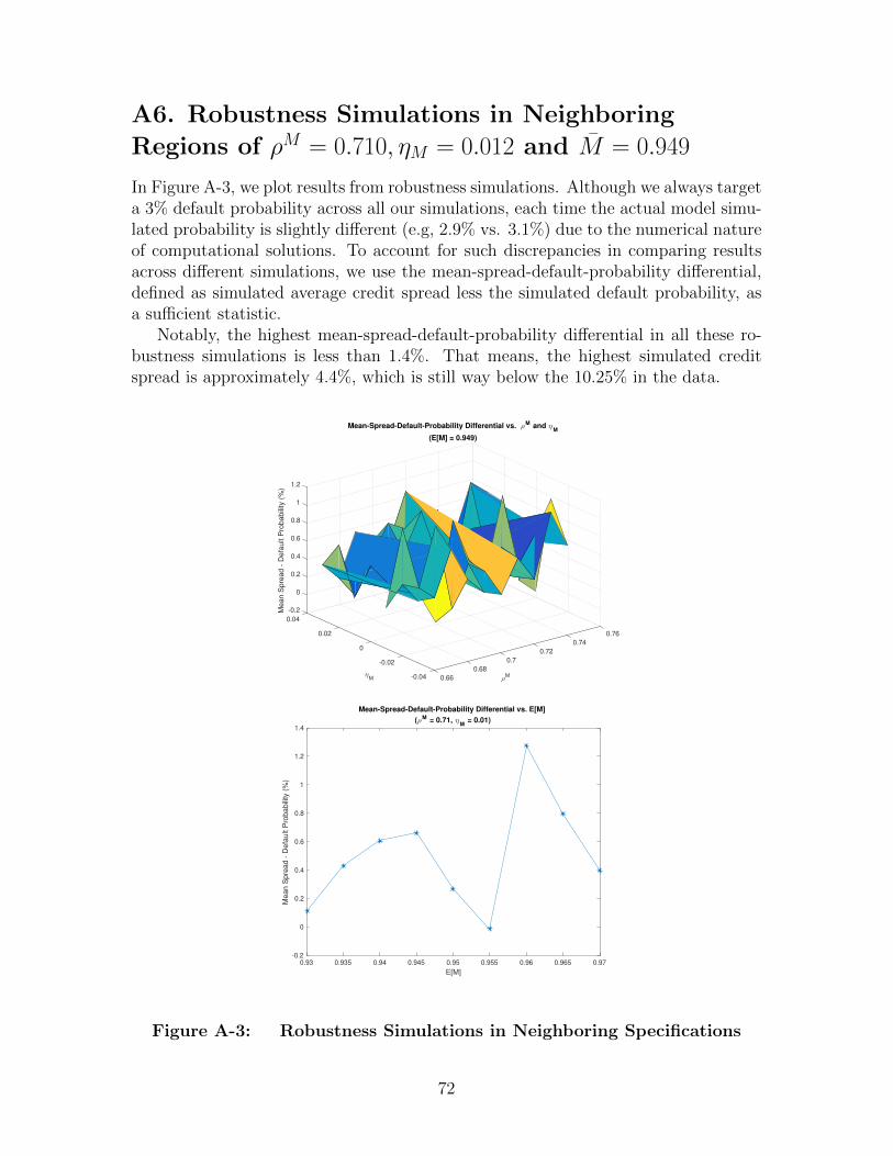
A6. Robustness Simulations in Neighboring

Regions of ρM = 0.710, ηM = 0.012 and M = 0.949

In Figure A-3, we plot results from robustness simulations. Although we always targeta 3% default probability across all our simulations, each time the actual model simu-lated probability is slightly different (e.g, 2.9% vs. 3.1%) due to the numerical natureof computational solutions. To account for such discrepancies in comparing resultsacross different simulations, we use the mean-spread-default-probability differential,defined as simulated average credit spread less the simulated default probability, asa sufficient statistic.

Notably, the highest mean-spread-default-probability differential in all these ro-bustness simulations is less than 1.4%. That means, the highest simulated creditspread is approximately 4.4%, which is still way below the 10.25% in the data.

-0.2

0.04

0

0.2

0.4

0.02 0.76

Mean S

pre

ad -

Defa

ult P

robabili

ty (

%)

0.6

0.74

0.8

Mean-Spread-Default-Probability Differential vs. ρM and ηM

(E[M] = 0.949)

ηM

0

1

0.72

ρM

1.2

0.7-0.020.68

-0.04 0.66

0.93 0.935 0.94 0.945 0.95 0.955 0.96 0.965 0.97

E[M]

-0.2

0

0.2

0.4

0.6

0.8

1

1.2

1.4

Mean S

pre

ad -

Defa

ult P

robabili

ty (

%)

Mean-Spread-Default-Probability Differential vs. E[M]

(ρM = 0.71, ηM

= 0.01)

Figure A-3: Robustness Simulations in Neighboring Specifications

72

A7. Historical Default Episodes with

Hyper-Inflations

In Figure A-4, we re-plot Figure II-1 using alternative default criteria that account forde facto defaults through hyper-inflations. Notably, 400% inflation rate is defaultingon approximately 80% of outstanding domestic bonds that are largely issued in do-mestic currencies, and 100% inflation rate loosely corresponds to an implicit defaulton 50% of existing domestic bonds.

Sovereign Default and Inflation Episodes(70 Countries, Inflation >=400%)

1800-2010

Domestic Only(w/ Inflaton): 17%(45)

External Only: 76%(196)

Twin Defaults(w/ Inflation): 7%(17)

Sovereign Default and Inflation Episodes(70 Countries, Inflation >=400%)

1960-2010

Domestic Only(w/ Inflation): 21%(24)

External Only: 71%(80)

Twin Defaults(w/ Inflation): 7%(8)

Source: Self-computations based on Reinhart and Rogoff (AER,2011)

Sovereign Default and Inflation Episodes(70 Countries, Inflation >=100%)

1800-2010

Domestic Only(w/ Inflaton): 26%(75)

External Only: 68%(195)

Twin Defaults(w/ Inflation): 6%(18)

Sovereign Default and Inflation Episodes(70 Countries, Inflation >=100%)

1960-2010

Domestic Only(w/ Inflation): 27%(33)

External Only: 66%(80)

Twin Defaults(w/ Inflation): 7%(8)

Source: Self-computations based on Reinhart and Rogoff (AER,2011)

Figure A-4: Historical Default Episodes with Hyper-Inflations

73

A8. Historical Default Episodes at Country-Level

In Figure A-5, we plot summary statistics of historical default episodes for countriesthat are among the top 15 most frequent defaulters witin the sample. Notably,external defaults are universally more common than domestic defaults for every singleone in the list.

Top Serial Sovereign Defaulters1800-2010

0 2 4 6 8 10 12

Source: Self-computations based on Reinhart and Rogoff (AER,2011)

Brazil

Chile

Ecuador

Peru

Uruguay

Turkey

Venezuela

Argentina

CostaRica

DominicanRepublic

Mexico

Russia

Austria

Ghana

Guatemala

Domestic OnlyTwin DefaultsExternal Only

Top Serial Sovereign Defaulters1960-2010

0 2 4 6 8 10 12

Source: Self-computations based on Reinhart and Rogoff (AER,2011)

Ghana

Brazil

Chile

Peru

Uruguay

Argentina

Indonesia

Turkey

Venezuela

Angola

Bolivia

CostaRica

DominicanRepublic

Ecuador

Nigeria

Domestic OnlyTwin DefaultsExternal Only

Figure A-5: Top Serial Defaulters

74

A9. Solution Algorithm

To computationally solve for the equilibrium solutions, we follow a standard valuefunction iteration procedure formally outlined as below.

1. Guess initial equilibrium discount bond prices qd0 and qe0.

2. Guess initial value functions V o0 , V d

0 , V e0 , and V b

0 .

3. Compute optimal policies in Be, bdh, and bdf for the case of repaying bothdomestic and external debts, taking bond discount prices qd0 and qe0 and initialguess of continuation value V o

0 as given.

4. Compute next-iteration V r1 , taking optimal policies in Be, bdh, and bdf and

continuation value V o0 as given.

5. Repeat steps 3 and 4 to compute next-iteration V e1 and V d

1 , as well as theirrespective optimal default policies DD0(bdh, bdf , Be) and ED0(bdh, bdf , Be), andtheir respective optimal policies in Be, bdh, and bdf .

6. Compute next-iteration V b1 , taking V e

1 , V d1 , and V o

0 as given.

7. Compute next-iteration V o1 , and optimal default policies DD1(bdh, bdf , Be) and

ED1(bdh, bdf , Be), taking V b1 , V e

1 , V d1 and V r

1 as given.

8. Replace V o0 with the newly computed V o

1 , and repeat steps 3–7 until convergencein V o.

9. Compute new discount bond prices qd01 and qe01, taking optimal default policiesDD(bdh, bdf , Be) and ED(bdh, bdf , Be) as given.

10. Update discount bond prices qd1 = µqd0 + (1− µ) qd01, and qe1 = µqe0 + (1− µ) qe01.

11. Repeat steps 3-10 until convergence in prices qd and qe.

75

A10. U.S. Economic Landscape

In Figure A-6, we categorize all U.S. counties from the 48 contiguous states into tendeciles by the number of establishments per unit land area. In Figure A-7, we plotlocations of bank headquarters for all commercial banks with total assets ≥ $1 billionas of 2010 on top of Figure A-6.

Figure A-6: U.S. Economic Density at County-Level

Figure A-7: U.S. Economic Density at County-Level and Banks

76

A11. An Example of de novo Counties

To illustrate the concept of de novo counties using an example, we start from BB&TCorporation’s acquisition of First Virginia Banks completed on July 2, 2003. InFigure A-8, we plot a map of county-level footprints for the two merging banksright before the merger. Green counties denote those in which there were deposit-taking BB&T Corporation branches, yellow counties denote those in which therewere deposit-taking First Virginia Banks branches, and the red-shaded counties de-note those with an overlap. In this case, we sample all yellow counties as our denovo counties. Intuitively, these are the counties BB&T Corporation first enters intothrough the merger.

Figure A-8: Map of County-Level Bank Footprints

77