Contents lists available at ScienceDirect

Tectonophysics

journal homepage: www.elsevier.com/locate/tecto

Three-dimensional S-wave velocity model of the Bohemian Massif fromBayesian ambient noise tomography

Lubica Valentováa,*, František Galloviča, Petra Maierováb

a Department of Geophysics, Faculty of Mathematics and Physics, Charles University in Prague, V Holešovičkách 2, Prague 18000, Czech Republicb Center for Lithospheric Research, Czech Geological Survey, Klárov 3, Prague 1 11821, Czech Republic

A R T I C L E I N F O

Keywords:Ambient noise tomographyBayesian inversionBohemian MassifGeologic domains

A B S T R A C T

We perform two-step surface wave tomography of phase-velocity dispersion curves obtained by ambient noisecross-correlations in the Bohemian Massif. In the first step, the inter-station dispersion curves were inverted foreach period (ranging between 4 and 20 s) separately into phase-velocity maps using 2D adjoint method. In thesecond step, we perform Bayesian inversion of the set of the phase-velocity maps into an S-wave velocity model.To sample the posterior probability density function, the parallel tempering algorithm is employed providingover 1 million models. From the model samples, not only mean model but also its uncertainty is determined toappraise the reliable features. The model is correlated with known main geologic structures of the BohemianMassif. The uppermost low-velocity anomalies are in agreement with thick sedimentary basins. In deeper parts(4–20 km), the S-wave velocity anomalies correspond, in general, to main tectonic domains of the BohemianMassif. The exception is a stable low-velocity body in the middle of the high-velocity Moldanubian domain andhigh-velocity body resembling a promontory of the Moldanubian into the Teplá-Barrandian domain. The mostpronounced (high-velocity) anomaly is located beneath the Eger Rift that is a part of a Tertiary rift system acrossEurope.

1. Introduction

Earth's ambient seismic noise, generated mainly by processes inoceans and atmosphere, has been present in seismic records to distressand vex seismologists for many years. It was only recently that therecordings of the ambient noise were recognized to be useful: by cross-correlating long series of noise recordings between two stations theGreen's function between them may be obtained (Campillo and Paul,2003; Shapiro and Campillo, 2004). The Greens' functions representresponse in a given location to an impulsive source in another point andthus contain purely information about the seismic properties of themedia between the two points. Therefore, it is natural to use them intomography.

In the first ambient noise tomography applications, the results werepresented by a set of 2D group (and later phase) velocity dispersionmaps obtained by the inversion of traveltimes between station pairs foreach period separately. The dispersion maps for various regions wereestimated: US – Shapiro et al. (2005) and Lin et al. (2008), New Zealand– Lin et al. (2007), Korean peninsula – Cho et al. (2007), Europe – Yanget al. (2007), etc. They show good correlations with known geologicstructures and may be used for preliminary interpretations.

The phase/group velocity dispersion maps at a set of periods can bealso translated into a 3D velocity model. This has been done on variousscales, from global (Haned et al., 2015; Nishida et al., 2009) to regional(Badal et al., 2013; Li et al., 2010; Pang et al., 2016), up to local net-works, for example, around volcanos (Matos et al., 2015; Obermannet al., 2016; Ryberg et al., 2016; Spica et al., 2015). The ambient noisetraveltime dataset may be also combined with another dataset, for in-stance, with teleseismic traveltimes to increase the resolution at greaterdepths (e.g., Yang et al., 2008; Ouyang et al., 2014; Guo et al., 2016;Rawlinson et al., 2016), or with receiver functions beneath the stationsto improve sensitivity to interfaces in the velocity structure (e.g., Bodinet al., 2012; Guo et al., 2015; Shen et al., 2012; Růžek et al., 2012). Theambient noise tomography has proved useful also for broader applica-tions, such as tomography of ocean ridges using a network of ocean-bottom seismometers (Mordret et al., 2014; Zha et al., 2014) or as-sessment of seismic anisotropy (Guo et al., 2012; Shirzad and Shomali,2014).

Inversion of surface wave dispersion data into a 3D velocity modeltraditionally employs a two-step approach. In the first step, the period-dependent traveltimes based on dispersion curves measured betweentwo points are inverted into phase/group velocity dispersion maps. In

http://dx.doi.org/10.1016/j.tecto.2017.08.033Received 30 May 2017; Received in revised form 26 July 2017; Accepted 27 August 2017

* Corresponding author.E-mail address: valent@karel.troja.mff.cuni.cz (L. Valentová).

Tectonophysics 717 (2017) 484–498

Available online 31 August 20170040-1951/ © 2017 Elsevier B.V. All rights reserved.

MARK

the second step, the dispersion curves on a regular grid are extractedand inverted for each grid point independently into a set of 1D velocitymodels. These 1D models are then assembled into a final 3D velocitymodel. In this second step, various techniques are employed. Standarddeterministic approach is based on iterative linearized least square in-version (e.g. Li et al., 2010; Luo et al., 2012; Matos et al., 2015; Porrittet al., 2016). However, stochastic approaches based on Monte Carlo(MC) methods are becoming more popular. The great advantage of theMC methods is that the result is not represented by a single model, butby a rather large set of models sampling the posterior probabilitydensity function. This is essential in the case of multimodal probabilitydensity functions, when the solution is nonunique and should not berepresented by one particular model. The MC methods are able to ex-plore several areas of model parameter space where the probabilitydensity function attains significant values. One may either extract co-herent properties of the models (e.g., by model averaging), or assessuncertainties and correlations between the retrieved model parameters.Moreover, the MC solutions are numerically more stable – one does nothave to deal with matrix inversion as in the case of the linearized in-version. Various MC methods have already been employed in ambientnoise tomographic applications, for example, simulated annealing(Spica et al., 2014, 2015), neighborhood algorithm (Gao et al., 2011;Mordret et al., 2014) or other MC search algorithms (Guo et al., 2015;Jiang et al., 2016, 2014). In our application, we employ another MCtechnique called parallel tempering, which was introduced into geo-physical problems only recently by Sambridge (2014). The method iswell balanced between fast convergence and avoiding entrapment inlocal maxima of the probability density function.

In the traditional two-step inversion, a 3D model is compiled fromseparately inverted 1D vertical models defined on a regular horizontalgrid. The 1D models may be defined by a large number of velocitylayers (Li et al., 2010; Pang et al., 2016; Porritt et al., 2016) but also in atransdimensional way, where the number of model parameters is re-garded as a hyperparameter (e.g., Young et al., 2013a,b; Pilia et al.,2015; Galetti et al., 2017). However, we take a different approach:instead of performing 1D inversion for each point of the dispersion mapseparately, the 3D model is parametrized using fixed layers and theinversion is carried out for all the model parameters simultaneously.

We apply the methodology to the Bohemian Massif – a remnant ofthe Variscan orogen with a complex structure and history (see Fig. 1a)summarized in Section 2. The input data consist of phase velocity dis-persion curves between the station pairs in periods 4–20s obtained from

ambient-noise cross-correlations – see Section 3. In Section 4, we out-line the methods applied in our problem. Then, we present the results ina form of dispersion maps and S-wave velocity model in Section 5. As aresult of the limited period range of the dispersion data, the resultingmodel is bound to recover only the top 25 km of the Bohemian Massifcrustal structure. In Section 6, the models are interpreted in terms ofknown geologic structures and compared with models obtained byother authors. The work represents the first 3D ambient noise tomo-graphy of the Bohemian Massif. Moreover, since the inversion is per-formed in the Bayesian framework, the model uncertainty is estimatedas well.

2. Bohemian Massif

2.1. Tectonic setting

The Bohemian Massif (Fig. 1a) is a relic of the European Variscanorogenic belt that formed ∼400–300 Myr ago as a result of con-vergence between Gondwana and Laurussia (Franke, 2000; Matte,2001). It consists of several major tectonic domains with differenthistory and dominant rock types (for overview see Schulmann et al.,2009). Most of them originally formed a part of the Gondwanan activemargin, and separated as continental micro-plates during the Late-Cambrian–Ordovician times. When the motion of the plates changedand the region between Gondwana and Laurussia was closing, theSaxothuringian domain was a part of the subducting plate (e.g., Franke,2000). It recorded significant deformation and metamorphism withintensity increasing towards its south-eastern boundary where theoceanic suture was located. The most prominent relic of the suture isthe Mariánské Lázně Complex that contains mafic rocks buried along acold geotherm in a sequence typical for closure of an oceanic domain(Beard et al., 1995).

The Teplá-Barrandian domain was a part of the upper plate duringthe orogeny and preserved the pre-Variscan upper crust including se-dimentary sequences affected only by low-grade deformation and me-tamorphism (Drost et al., 2004). The south-eastern margin of the Teplá-Barrandian domain was intruded by magmatic rocks together formingthe Central Bohemian Plutonic Complex. The composition of theserocks corresponds to melting of mantle variably enriched by crustalcomponent, which is typical for a magmatic arc above a subductionzone (Janoušek et al., 2000).

The Moldanubian domain was a continuation of the Teplá-

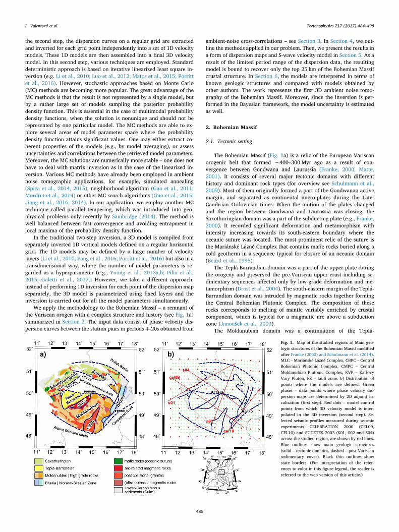
Fig. 1. Map of the studied region: a) Main geo-logic structures of the Bohemian Massif modifiedafter Franke (2000) and Schulmann et al. (2014).MLC – Mariánské Lázně Complex, CBPC – CentralBohemian Plutonic Complex, CMPC – CentralMoldanubian Plutonic Complex, KVP – KarlovyVary Pluton, FZ – fault zone. b) Distribution ofpoints where the models are defined: Greenpluses – data points where phase velocity dis-persion maps are determined by 2D adjoint lo-calization (first step). Red dots – model controlpoints from which 3D velocity model is inter-polated in the 3D inversion (second step). Se-lected seismic profiles measured during seismicexperiments CELEBRATION 2000 (CEL09,CEL10) and SUDETES 2003 (S01, S02 and S04)across the studied region, are shown by red lines.Blue outlines show main geologic structures(solid – tectonic domains, dashed – post-Variscansedimentary cover). Black thin outlines showstate borders. (For interpretation of the refer-ences to color in this figure legend, the reader isreferred to the web version of this article.)

L. Valentová et al. Tectonophysics 717 (2017) 484–498

485

Barrandian domain during the orogeny, but it was affected by medium-to-high grade metamorphic conditions (Schulmann et al., 2009). Thecontrasting character of the two adjacent domains results from theirrespective vertical displacement at a shear zone that developed in theweakened magmatic arc region (the Central Bohemian Plutonic Com-plex, Dörr and Zulauf, 2010). Erosion of the elevated Moldanubiansurface then led to exposure of its middle and lower crust. The centralpart of the Moldanubian domain also contains a large accumulation ofplutonic bodies that formed by crustal melting at the late stage of theorogeny – the Central Moldanubian Plutonic Complex (Finger et al.,2009).

The easternmost part of the Massif is the Brunia (or Brunovistulian)domain. Along the margin with the Moldanubian domain, the Brunia-derived rocks were strongly deformed and metamorphosed within theso-called Moravo-Silesian Zone as a result of thrusting of Brunia un-derneath the Moldanubian domain (see references in Schulmann et al.,2009). The interpretation of the Bouguer gravity anomaly suggests thatthe Brunia basement continues 50–70 km west of its surface margin andis covered only by a thin layer of Moldanubian rocks (Guy et al., 2011).In addition, westward continuation of Brunia on the level of the mantlelithosphere was inferred from the seismic anisotropy (Babuška andPlomerová, 2013). The Brunia basement is covered by Variscan as wellas younger sedimentary sequences (Kalvoda et al., 2008).

During the collapse of the Variscan orogen, its elevated topographywas subject to extension and gradual erosion which resulted in for-mation of several Permo–Carboniferous sedimentary basins. Later on inthe Permian, subsidence of the Polish basin started eventually leadingto formation of a several kilometers thick sedimentary cover north ofthe Bohemian Massif.

At∼70 Myr ago, the onset of the Alpine orogeny led to activation ofthe Elbe Fault Zone, subsidence of the surrounding area and formationof the Bohemian Cretaceous Basin (Uličný et al., 2009). Its today'sthickness reaches 1 km and it covers a significant part of the Teplá-Barrandian domain. North-east of the Elbe Fault Zone, the Sudetesdomain is located showing similar characteristics as the Saxothuringiandomain.

The Alpine orogeny further reactivated existing fractured zonesacross Europe by rifting and related volcanism and sedimentation(Dèzes et al., 2004). In the Bohemian Massif the Eger Rift was activatedalong the Saxothuringian–Teplá-Barrandian boundary showing recentregular earthquake swarms, CO2 emanations and elevated surface heatflow (Čermák, 1994; Cloetingh et al., 2010). Various seismic studiespointed to anomalous character of the crust and to asthenosphericupdoming beneath the Eger Rift (e.g., Heuer et al., 2006; Geissler et al.,2005; Plomerová et al., 2007; Hrubcová and Środa, 2015). The Alpineorogeny also shaped the southern margin of the Bohemain Massif that isnow covered by Alpine-Carpathian foreland basins and overthrust bythe Western Carpathians in the east.

2.2. Previous tomographic studies

Due to its complex history and structure, the region of the BohemianMassif has been subject to many seismologic studies starting from the80s (see Novotný and Urban, 1988). Most of the recent crustal studiesuse active experiments along profiles, such as CELEBRATION 2000 andSUDETES 2003. The applied tomographic methods result in 2D verticalmainly P-wave velocity models. The crustal models along the activeexperiment profiles (see also Fig. 1b) were determined: CEL09 crossingmost of the tectonic domains (Hrubcová et al., 2005; Novotný, 2012),CEL10 along the Moravo-Silesian Zone (Hrubcová et al., 2008), S01along the Eger Rift (Grad et al., 2008; Novotný et al., 2009), S04 almostparallel with CEL09 (Hrubcová et al., 2010). Models along severalprofiles concentrating on the Bohemian Massif were acquired by Růžeket al. (2007) and in the Sudetes by Majdański et al. (2006). The modelsshow some common basic characteristics of the Bohemian Massif:firstly, there is very thin or no sedimentary coverage on the Bohemian

Massif in the seismic data. Secondly, one can divide the crust into upperand lower one with P-wave velocity contrast of ∼0.5 km/s in almost alltectonic domains. Usually, both upper and lower crust is stronglyhomogenized with low vertical gradient. In the subsurface parts, thehigh-velocity bodies are correlated with mafic intrusions whereas thelow-velocity anomalies with granitic structures. In the upper crust, thedistinct anomalies were found in the area of the Eger Rift. The Mol-danubian domain shows higher P-wave velocities compared to theother domains representing the high-grade rocks. The Moho beneaththe Bohemian Massif reaches to depths 30–40 km.

Thanks to numerous experimental data, tomographic inversion into3D models was performed as well, for example, focused on the Moravo-Silesian region by Růžek et al. (2011), or over larger regions: P-wavevelocity model for the Sudetes region by Majdański et al. (2007) or S-wave velocity model of the Bohemian Massif and Alps by Behm (2009).These models show good correlation of the subsurface structures withknown geology. 3D P- and S-wave local velocity model of West Bo-hemia using not only experimental but also local earthquake data wasacquired by Růžek and Horálek (2013). In this model, the areas withlow Poisson ratio correlate with focal zones of the West-Bohemiaearthquakes. Several crustal models were compiled together into a 3Dmodel using different interpolation techniques by Karousová et al.(2012). The map of the Moho depth extracted from this model showssignificant crustal thickening in the southern part of the Moldanubiandomain and in the Brunia domain.

The crustal domains of the Bohemian Massif were found to continuealso in the mantle lithosphere where they are characterized by differentP-wave anisotropy patterns (Babuška and Plomerová, 2013; Plomerováet al., 2005).

1D S-wave velocity models beneath the stations in the BohemianMassif are provided by receiver function studies (e.g., Wilde-Piórkoet al., 2005; Geissler et al., 2012; Heuer et al., 2006). Receiver functionstudies combined with ambient noise cross-correlation data focused onthe crust of the Bohemian Massif were performed by Růžek et al.(2012). Beneath the stations located in different tectonic domains, thecoherent properties in the receiver functions may be found. Except forthe Moho deepening under the Moldanubian, the Moho updoming wasfound not only beneath the Eger Rift, but also in the area of the Bo-hemian Cretaceous Basin where it was connected to the tectonic ac-tivity along the Elbe Fault Zone.

The stepping stone for our work are the ambient noise cross-corre-lation studies by Růžek et al. (2016) who investigated the S-wave ve-locity properties for different domains of the Bohemian Massif. Thedomains show slightly different characteristics, but the variabilitywithin each domain is comparable with the differences among them.

In our work, we utilize these ambient noise cross-correlation data toobtain 3D S-wave crustal velocity model of the whole Bohemian Massif.

3. Data

We adopt inter-station dispersion curves estimated independentlyfor all components (transverse T, radial R and vertical Z), which wereextracted from ambient noise cross-correlations by Růžek et al. (2016).The stations used in the processing are a) permanent stations belongingeither to the Czech Regional Seismological Network (CRSN) or theVirtual European Broadband Seismological Network (VEBSN); b) tem-porary stations operating within experiments BOHEMA I–III or PASSEQ(Babuška et al., 2005; Plomerová et al., 2003; Wilde-Piórko et al.,2008); c) stations belonging to adjacent regional networks (Saxonianand Bavarian). The total number of stations is 72. The selected stationsare equipped with broadband sensors and the noise measurements spanover a time period of 12 years. To extract dispersion curves between thestations, the cross-correlations of the preprocessed noise between pairsof stations were calculated. More details on the method and resultinginter-station dispersion curves can be found in Růžek et al. (2016). Theresulting inter-station dispersion curves range between periods 4 and

L. Valentová et al. Tectonophysics 717 (2017) 484–498

486

20 s. In the inversion, we employ only phase velocity dispersion curveswith high signal-to-noise ratio in the cross-correlation function.

Fig. 2 shows the station and data coverage for the R component. Thenumber of measured traveltimes is almost 700. Note, that for the othertwo components, the data coverage is even better due to generallyhigher-quality cross-correlation functions.

4. Methods

The inversion method is derived from the traditional two-step ap-proach described in Section 1. In the first step, we invert the inter-station dispersion curves separately for the selected periods into a 2Dregular grid (so-called phase velocity dispersion maps) using 2D adjointmethod. For the second step, we perform the inversion of the dispersionmaps into a 3D S-wave velocity model in a Bayesian framework.

4.1. Adjoint localization

To obtain phase velocity dispersion maps, we apply 2D adjoint in-version (Fichtner et al., 2006; Tape et al., 2007; Tromp et al., 2005) tointer-station dispersion curves for selected periods. The station cov-erage as well as the number of dispersion traveltimes in the studiedregion may be considered sufficient for the tomographic problem (seeFig. 2).

The adjoint method belongs to iterative gradient methods of themisfit minimization. The misfit considered in our problem is the L2norm of the cross-correlation traveltime differences. The misfit gradient(i.e., the derivative of the misfit with respect to the model parameters)is calculated using one forward and one so-called adjoint calculation. Inour problem, the adjoint calculation is represented by backpropagationof so-called adjoint wavefield from the receivers back to the sources(Peter et al., 2007; Tape et al., 2007). The forward and adjoint wave-fields are then combined into finite-frequency or sensitivity kernels,which emphasize areas with increased values of the misfit gradient.

The greatest advantage of the adjoint method is that it accounts forthe finite-frequency effects of the wave propagation. Nevertheless, themethod requires regularization, for example, by means of Gaussiansmoothing that is applied to the calculated sensitivity kernels (Peteret al., 2011; Tape et al., 2007, 2010). The width of the Gaussian

smoothing function as well as the optimal number of iteration steps wasdetermined using preliminary synthetic tests with actual data noise(Valentová et al., 2015). More details are to be found in Section 4.3.

4.2. Bayesian inversion

We apply a Bayesian approach to solve the second stage of the in-verse problem. The result of the inversion is represented by a set ofmodel samples obtained by a random walk according to the posteriorPDF. The method is appropriate for non-linear problems, such as in-version of dispersion curves. Moreover, from the model samples onemay estimate not only the best or the mean model, but also its un-certainty.

The posterior PDF is defined as conditional PDF on model parameterspace after measurement of data d is acquired (e.g., Tarantola andValette, 1982; Mosegaard and Tarantola, 1995; Tarantola, 2005). Thisis usually expressed using the Bayes theorem:

=m dm d m

dp

p pp

( | )( ) ( | )

( ),

(1)

where p(m) is the model parameter PDF which is independent on thedata measurement (i.e., prior PDF, denoted pprior). Conditional prob-ability of observing data given model m, p(d|m), is so-called likelihoodfunction. The likelihood function for measured data d=dobs containsstatistical information on the data measurement error, but may alsoinclude modeling error. However, the information on the modelingerror is usually difficult to estimate or negligible compared to themeasurement error, and is therefore not assumed. The posterior PDF asa function of model parameters m for measured data d=dobs can berewritten as

=m m d mp k p p( ) ( ) ( ),prior obs (2)

where k is a PDF normalization constant.Usually, the data PDF is considered in a form of Gaussian distribu-

tion, then

∝ −d m mp S( | ) exp( ( )),obs (3)

where S(m) defines misfit between measured data dobs and syntheticscalculated using a theoretical relation g(m) with Gaussian covariancematrix Cd:

= − −−m d g m d g mS C( ) ( ( )) ( ( )).Tobs d

1obs (4)

To draw samples from the model space according to the posteriorPDF, the Markov chain MC random walker is employed. In each step ofthe chain, the model parameters are randomly perturbed consideringGaussian probability function. The new (proposed) model is accepted orrejected based on the Metropolis algorithm: if the posterior PDF of theproposed model is higher, the model is accepted; if the PDF is lower, themodel may be still accepted with some probability. The acceptance ratedepends on the width of the Gaussian generating the perturbations, i.e.,the perturbation of the misfit. To increase the efficiency of the samplerwe apply a method called parallel tempering (PT, Sambridge, 2014).The PT algorithm is similar to the better-known simulated annealing, asit introduces modification of the PDF by an additional parameter calledtemperature T. The modified PDF p(m,T) is given by

⎜ ⎟⎛⎝

⎞⎠

= ⎛⎝

− ⎞⎠

m m mp T k p ST

, ( )exp ( ) .prior(5)

The samples are drawn following this modified PDF assuming multiplevalues of the temperature T.

For high temperatures, the PDF becomes smooth (note that for T→∞, p→pprior). For low temperatures, the PDF maxima are more pro-nounced and as T → 0, PDF converges to δ function located in theglobal maximum (i.e., global minimum of S(m)). For T=1, the mod-ified PDF equals to the original PDF. During the simulated annealing,

Fig. 2. Station configuration of the investigated area. The station-pairs with measuredphase-velocity dispersion curve for the R component are connected by lines. The selectedstations (marked by circle) serve as source for the adjoint inversion.

L. Valentová et al. Tectonophysics 717 (2017) 484–498

487

temperature T gradually decreases from high values to lower values sothat the sampler gradually concentrates into areas with higher PDFvalues. In the PT method, multiple Markov chains each with differenttemperature sample the model parameter space simultaneously. Thechains with lower temperature values sample locally areas of PDFmaxima, whereas chains with higher temperatures are able to escapethe local maxima of PDF. Moreover, two chains can exchange theirtemperature values between the chain advances. The probability thattwo chains (denoted [mi,Ti] and [mj,Tj]) swap their temperatures (re-sulting in [mi,Tj] and [mj,Ti]) is given by the Metropolis-Hastings cri-terion. This condition ensures, that the subset of samples for tempera-ture T=1 represents sampling of the original untempered PDF p(m).The PT algorithm is well balanced between efficiency and stability forcomplex multimodal PDFs (Sambridge, 2014). Another advantage isstraightforward parallelization of the sampling computer code.

4.3. Implementation details

In the 2D adjoint localization, the regularization is applied primarilyby means of Gaussian smoothing of the sensitivity kernels and by thenumber of iterations. The regularization parameters are estimated bysynthetic tests using a smooth and a complex model to examine relia-bility of both long-scale and short-scale features. For the 20 s Love datainversion, the width of the Gaussian smoothing function is set to100 km with iterations stopping at 6th step (for more information andrelated synthetic tests see Valentová et al., 2015). For other periods(both Love and Rayleigh datasets), the size of the Gaussian functionscales with the corresponding wavelength.

The phase velocity dispersion maps are calculated for periods (4, 6,8, 10, 12, 16, 20) s in the first stage and serve as input data in thesecond step of the inversion in which the Bayesian approach is applied.We extract dispersion curves in a selected 2D regular grid of data points(green pluses in Fig. 1b). The 3D velocity model is represented by a setof vertical 1D layered models on a regular horizontal grid of modelcontrol points (red dots in Fig. 1b). The spacing of the data and modelcontrol points is 16 km and 50 km, respectively. In each model controlpoint, we assume 7 layers above a halfspace with interfaces at depths of2, 4, 8, 12, 18, 24, and 32 km. Although the model is parametrized in3D, the synthetic dispersion curves are calculated for computationalreasons assuming 1D layered model at each data point. In the MCmethods, the forward problem is calculated numerous times and thus afast solver (such as 1D) is necessary. We employ the code VDISP whichis based on a matrix method using Thomson-Haskell and Watson'smatrices for Love and Rayleigh waves, respectively (Novotný, 1999). Toobtain a 1D layered model for the synthetic dispersion curve calcula-tion, the model is interpolated in each layer from the model controlpoints into the data grid points by cubic spline interpolation.

The Bayesian inversion is regularized by the adopted parametriza-tion. Firstly, the number of layers is rather low and with fixed thick-nesses; the number of model control points is kept lower than thenumber of data points. Furthermore, the model is interpolated into thedata points using smooth functions (cubic splines).

The Bayesian inversion employs the PT algorithm to sample theposterior PDF. As the model prior information pprior(m) we use homo-geneous PDF on a selected interval for all model parameters, in parti-cular between 1 and 15 km/s. Another constraint on the model para-meters is the requirement of a nonnegative velocity gradient with depthfor each model control point. For simplicity, the data covariance matrixCd is assumed to be diagonal with standard deviation corresponding toerror of dispersion maps (see Section 5.1).

We run the computations in parallel on 12–24 CPUs, the tempera-ture T ranges between 1 and 50. To remove the dependency of Markovchains on the starting model, we introduce long burn-in phase (10ksteps) when the accepted models are not saved. The main (post-burn)phase is stopped when the sampler appears to have converged on themodel space (i.e., no improvement in model space sampling occurs with

further thousands of chain steps). Only the samples from chains attemperature T=1 accepted every 100th step are saved and furtherprocessed. The resulting number of samples from the posterior PDFexceeds 1 million.

5. Results

In the first step, the inter-station dispersion curves were inverted foreach period separately by the 2D adjoint method. The results are re-presented by a set of phase velocity maps in Section 5.1.

In Section 5.2, we present the results of the Bayesian inversion ofthe dispersion maps into a 1D S-wave velocity model (and vp/vs) usingdifferent datasets and assumptions. The 1D Bayesian model of the Bo-hemian Massif reflects its average structure. Moreover, with the help ofsynthetic tests we discuss to what extent the variance in the 1D velocitymodel parameters contains also variability due to the 3D structures.

In Section 5.3, the results of the Bayesian inversion of the dispersionmaps into a 3D model is presented as 2D depth-slices for both absoluteand relative S-wave velocities, as well as horizontal variations of the vp/vs ratio. The correlations of the results with geology are discussed inSection 6.

5.1. Phase velocity maps

Fig. 3 shows the inverted phase velocity dispersion maps for eachperiod as obtained from the three components individually: Love (T)and both Rayleigh (R and Z). The perturbations in phase velocities areshown with respect to average values specified on the right side of eachmap.

We treat the dispersion curves for R and Z component as two in-dependent datasets, so that by comparing the resulting models we getinsight into the accuracy of the first part of the inversion. Regarding theaverage models, both components give very similar results. Contrarily,the phase-velocity perturbations of the R and Z component, althoughsimilar in some features, differ in some details as well.

We use differences between both Rayleigh dispersion maps to esti-mate the error of the dispersion maps. The RMS of the differencesranges between 0.10–0.15 s for different periods, which agrees wellwith the value of 0.14 s estimated from Rayleigh phase velocity dif-ferences between inter-station pairs by Růžek et al. (2016).

5.2. 1D velocity model

Here, we apply our stochastic MC inversion to obtain a re-presentative 1D layered velocity model for the real dataset. We as-semble data from all phase velocity maps, excluding points where theinitial velocity remains unchanged (i.e., there is no sensitivity of thedata on the velocity structure).

1D inversion is computationally cheap (≈4 h on 8 CPUs) and thusmay be used with the help of synthetic 1D tests to investigate propertiesof the inverse problem. The 1D inversions were performed employingdifferent datasets: only Love phase velocities or all-component phasevelocities. The 1D model is composed of 2 km thick layers down to32 km and a halfspace. Furthermore, the addition of the vp/vs modelparameter to 1D S-wave velocity parameters was examined.

Fig. 4a shows results of Love phase velocity inversion into a 1D S-wave velocity model. The model appears to have a relatively wide butunique maximum. This shows that although the result is stable, eitherthe data sensitivity to the S-wave velocity model is low or the 1D modelis inappropriate to represent the dataset due to the actual higher spatialvariability of the true velocity model, or both.

In Fig. 4b, we show the results of inversion of Love and Rayleighphase velocity dispersion data into a 1D layered S-wave velocity modelwith fixed vp/vs=1.57. By increasing the number of data, the varianceof the model parameters decreases. This suggests that the data from allcomponents are well represented by a common 1D S-wave velocity

L. Valentová et al. Tectonophysics 717 (2017) 484–498

488

model.Fig. 4c displays models obtained from the inversion of all compo-

nents into a 1D S-wave velocity model and an additional parameter –depth-independent vp/vs. The resulting S-wave velocity model is similarto the previous one (Fig. 4b), both in terms of the best model and thevariance. This shows that the inversion of the vp/vs parameter does notaffect the inversion of the S-wave velocity model much, except forslightly amplifying the velocity increase at ∼20 km. The obtained vp/vsratio has low variance and appears to be well resolved. However, byassuming depth-independent vp/vs, the inversion estimates vp/vs corre-sponding to the average over all depths. In general, the averagedparameter is better constrained than vp/vs at a given depth. Therefore, itmust not be interpreted as a low variability of the vp/vs of the real 3Dstructure.

From the 1D velocity models, it is difficult to distinguish betweenthe effects of data resolution and inherent variability due to the 3D

structure. To separate these two effects, we performed several synthetictests. The synthetic tests with both noiseless and noisy data were per-formed with similar setting as the real data inversion. The resultingvariance of the real data inversion is distinctly larger than that of thesynthetic tests. This suggests that the most of the 1D model variability isdue to the lateral inhomogeneity of the real crust.

5.3. 3D velocity models

The result of our Bayesian inversion consists of > 1 million PDFsamples (i.e., 3D models). To present the results, we display the meanmodel calculated from all models and the best model. The advantage ofthe mean model is that it presents only stable features. Therefore, themean model is typically smoother than any single model drawn by theMC sampler. The best model is shown as a representative model toexamine differences in properties between a single model and the

−10 −5 0 5 10

perturb [%]

T04s

12˚

12˚

14˚

14˚

16˚

16˚

48˚

48˚

50˚

50˚ 3.52

T06s

12˚

12˚

14˚

14˚

16˚

16˚

48˚

48˚

50˚

50˚ 3.56

T08s

12˚

12˚

14˚

14˚

16˚

16˚

48˚

48˚

50˚

50˚ 3.61

T10s

12˚

12˚

14˚

14˚

16˚

16˚

48˚

48˚

50˚

50˚ 3.69

T12s

12˚

12˚

14˚

14˚

16˚

16˚

48˚

48˚

50˚

50˚ 3.75

T16s

12˚

12˚

14˚

14˚

16˚

16˚

48˚

48˚

50˚

50˚ 3.86

T20s

12˚

12˚

14˚

14˚

16˚

16˚

48˚

48˚

50˚

50˚ 3.95

−10 −5 0 5 10

perturb [%]

R04s

12˚

12˚

14˚

14˚

16˚

16˚

48˚

48˚

50˚

50˚ 3.10

R06s

12˚

12˚

14˚

14˚

16˚

16˚

48˚

48˚

50˚

50˚ 3.16

R08s

12˚

12˚

14˚

14˚

16˚

16˚

48˚

48˚

50˚

50˚ 3.21

R10s

12˚

12˚

14˚

14˚

16˚

16˚

48˚

48˚

50˚

50˚ 3.27

R12s

12˚

12˚

14˚

14˚

16˚

16˚

48˚

48˚

50˚

50˚ 3.33

R16s

12˚

12˚

14˚

14˚

16˚

16˚

48˚

48˚

50˚

50˚ 3.48

R20s

12˚

12˚

14˚

14˚

16˚

16˚

48˚

48˚

50˚

50˚ 3.59

−10 −5 0 5 10

perturb [%]

Z04s

12˚

12˚

14˚

14˚

16˚

16˚

48˚

48˚

50˚

50˚ 3.11

Z06s

12˚

12˚

14˚

14˚

16˚

16˚

48˚

48˚

50˚

50˚ 3.16

Z08s

12˚

12˚

14˚

14˚

16˚

16˚

48˚

48˚

50˚

50˚ 3.20

Z10s

12˚

12˚

14˚

14˚

16˚

16˚

48˚

48˚

50˚

50˚ 3.26

Z12s

12˚

12˚

14˚

14˚

16˚

16˚

48˚

48˚

50˚

50˚ 3.32

Z16s

12˚

12˚

14˚

14˚

16˚

16˚

48˚

48˚

50˚

50˚ 3.46

Z20s

12˚

12˚

14˚

14˚

16˚

16˚

48˚

48˚

50˚

50˚ 3.57

Fig. 3. Phase velocity dispersion maps obtained by the 2D adjoint inversion for each period from all components: a) transverse T (i.e., Love wave), b) radial R c) vertical Z (both Rayleighwaves). The period increases from top to bottom (see legend). The model perturbations (color scale) are presented relative to mean phase velocity model, denoted for each map to theright in km/s. (For interpretation of the references to color in this figure legend, the reader is referred to the web version of this article.)

L. Valentová et al. Tectonophysics 717 (2017) 484–498

489

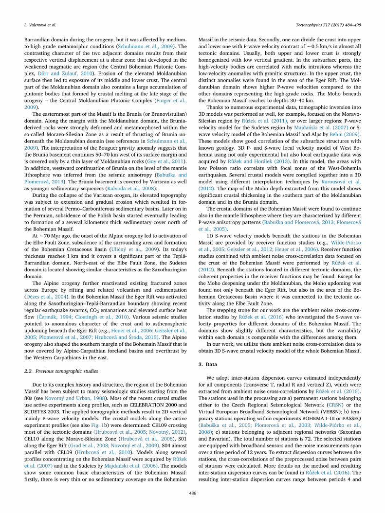
averaged one.Fig. 5 presents the depth-slices of the mean and the best 3D S-wave

velocity model. To better visualize its lateral variations, Fig. 6 showsthe same models but in terms of perturbations relative to the horizon-tally averaged model.

All models show increase of S-wave velocity with depth. Regardingthe lateral variations, both mean and best model share the most sig-nificant structures. The differences between them appear on smallerscales.

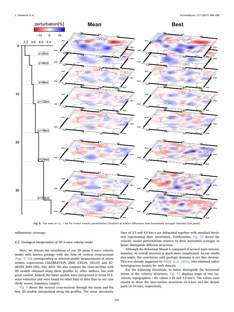
Simultaneously with S-wave velocities, we have performed the PTexploration also for the depth-independent vp/vs ratio. The reasons forthe vp/vs depth-independence are: a) poor resolution of vp/vs and b) toreduce the parameter space. The resulting mean model and its standarddeviation are shown in Fig. 7. Although, the range of the vp/vs ratio iswide (1.5–1.8), the standard deviation in recovered areas lies mostlybelow 0.05, suggesting strong horizontal structural variability of thisparameter.

5.4. Uncertainty of the 3D model

The greatest advantage of employing MC methods to solve the in-verse problem lies in the plurality of models representing the solution.As an example, Fig. 8a shows vertical 1D models in a model controlpoint located in the middle of our domain. From this example, we seethat the best resolved part in the inversion lies at depths of 2–18 km. Atgreater depths, the variance in the S-wave velocities is very high. It alsoappears that the PDF of the S-wave velocities in deeper parts as well asvp/vs ratio have 2 local maxima. We ascribe this to the undersampling ofthe PDF in the particular parameter domain. Also note that for modelcontrol points located at the boundaries of our domain, the overalluncertainty increases.

Uncertainty of the model along a profile can be estimated by stan-dard deviation of the mean model (Fig. 8b right). In general, the lowestuncertainty (as indicated also by the 1D models in Fig. 8a) is achieveddown to ∼20 km. However, the uncertainty changes also laterally

along the profile (between 1–2% for the well resolved part). Alter-natively, we visualize these changes via standard deviation of selectedS-wave velocity isolines (Fig. 8b left).

We emphasize that we should be extremely cautious when inter-preting the imaged structures below 25 km, where the model varianceincreases rapidly. In particular, our models are not suited for the searchof the Moho. The following geologic interpretation should be confinedto large-scale structures only. This limitation is a consequence of themethod applied, namely: a) employment of surface wave data, which isinherently sensitive to the averaged (smoothed) structures both hor-izontally and vertically, making it impossible to obtain velocity inter-faces; b) model parametrization – horizontal grid with relatively large(50 km) spacing; and c) averaging of great amount of single modelsgenerated by the MC inversion which produces stable but smoothstructures.

6. Discussion

6.1. Geological interpretation of dispersion maps and 1D S-wave velocityprofile

The result of the first part of the inversion – the phase-velocitydispersion maps – usually correlate well with known geology and areused for preliminary interpretation (e.g., Saygin and Kennett, 2010;Nicolson et al., 2012). In our dispersion maps (see Section 5.1, Fig. 3),there is a high velocity structure in the southern part of the domainpresent in almost all maps, which may be related to the Moldanubiandomain. Another stable high velocity anomaly, located in the center ofthe north-west border of the Czech Republic is found easily on maps forcomponents T and R for periods 8–16 s, where it is surrounded by lowvelocities. Moreover, this anomaly can be also tracked for the Z com-ponent. This anomaly is situated beneath the Eger Rift zone, where ahigh velocity body is usually found in the tomography (Alexandrakiset al., 2014; Grad et al., 2008; Mousavi et al., 2015; Růžek et al., 2007).For the shortest periods, the structures are much more complex and

Fig. 4. Results of the inversions of the phase velocity dispersionmaps into 1D layered models by the PT algorithm. The colorscale corresponds to the normalized PDF (nPDF) scaled by thePDF value of the best model (black dashed line). a) Inversion ofLove dispersion maps into a 1D S-wave velocity model. b)Inversion of all Love and Rayleigh dispersion maps into a 1D S-wave velocity model, vp/vs being fixed. c) Inversion of all Loveand Rayleigh dispersion maps into a 1D S-wave velocity model(left) and depth-independent vp/vs ratio (right). (For interpreta-tion of the references to color in this figure legend, the reader isreferred to the web version of this article.)

L. Valentová et al. Tectonophysics 717 (2017) 484–498

490

stable features present for all components are more difficult to de-termine. In the Elbe Fault Zone, one may observe a narrow low velocityanomaly for all maps at periods 4–6 s.

Before the inversion into 3D model, we performed Bayesian inver-sion of the dispersion maps into 1D S-wave velocity model and vp/vsratio (see Section 5.2, Fig. 4). This 1D model may be considered as arepresentative model of the Bohemian massif. In the near-surface part(depth less than 4 km), there is a moderate velocity gradient and re-latively large variance. This may point out to uneven sedimentary coverof the Bohemian Massif. The rest of the upper crust (from 4 to∼ 12 km)shows very low velocity gradient and a very low variance. This suggestsstrongly homogenized upper crust across the whole domain.

Around 20 km depth, there is a strong S-wave velocity increase in-dicating significant structural difference between the upper and lowercrust. The increased variance in these depths may be associated withthe high velocity gradient being laterally heterogeneous in the real

structure.Below 25 km, there is no significant velocity jump corresponding to

the Moho. Moreover, the variance in these depths decreases, namely inthe halfspace. This is due to the fact that the variance estimated for theS-wave velocity at these depths is only formal as it represents varianceof the S-wave velocity averaged over all depths below 32 km.Therefore, the obtained variance reflects neither vertical nor lateralvariability of the real 3D structure, and thus the Moho is not resolved inour model.

The Bohemian Massif shows low vp/vs value ∼1.6 indicating ratherrigid, consolidated material. The interpretation of the vp/vs horizontalperturbations in Fig. 7 is rather ambiguous as the uncertainty of thisparameter may be poorly estimated. In similar sense as the S-wavevelocity of the halfspace velocity mentioned above, the estimated vp/vscorresponds to the average over all depths. The increase in the northernpart (Sudetes), may be attributed to the presence of the thick

Fig. 5. Depth slices through the mean (left) and best (right) S-wave velocity models obtained by our 3D inversion using the PT algorithm. The layers are shown in the left. The areas withno station coverage are masked.

L. Valentová et al. Tectonophysics 717 (2017) 484–498

491

sedimentary coverage.

6.2. Geological interpretation of 3D S-wave velocity model

Here, we discuss the correlation of our 3D mean S-wave velocitymodel with known geology with the help of vertical cross-sections(Figs. 9, 10), corresponding to selected profile measurements of activeseismic experiments CELEBRATION 2000 (CEL09, CEL10) and SU-DETES 2003 (S01, S02, S04). We also compare the cross-sections with2D models obtained along these profiles by other authors, but withgreat caution. Indeed, the latter models were interpreted in terms of P-wave velocities and were based on other kind of data than in our case(body waves, frequency ranges).

Fig. 9 shows the vertical cross-sections through the mean and thebest 3D models interpolated along the profiles. The mean isovelocity

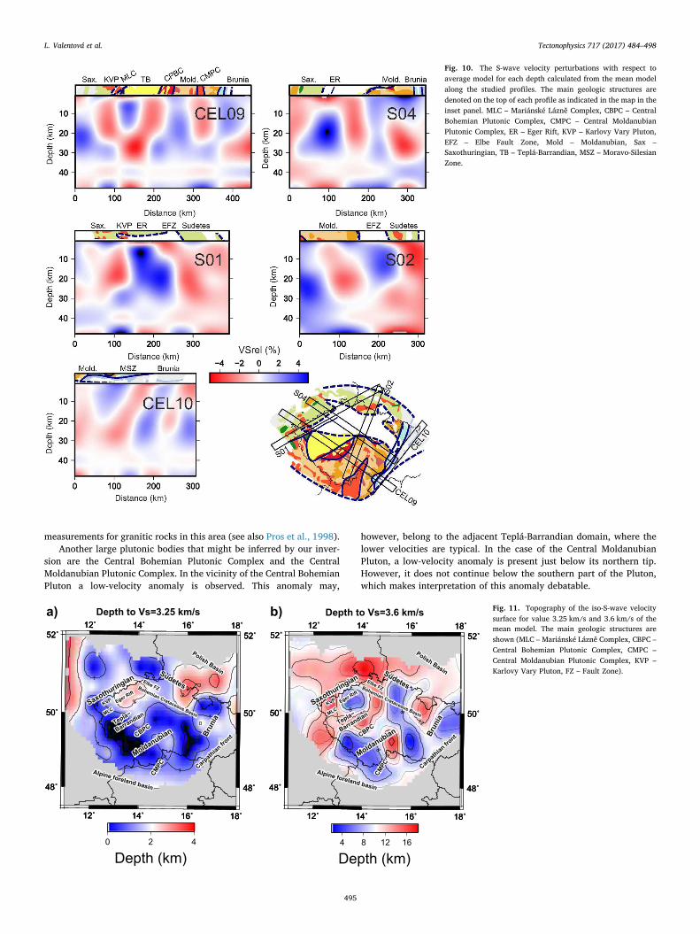
lines of 3.5 and 4.0 km/s are delineated together with standard devia-tion representing their uncertainty. Furthermore, Fig. 10 shows thevelocity model perturbations relative to their horizontal averages tobetter distinguish different structures.

Although the Bohemian Massif is composed of several main tectonicdomains, its overall structure is much more complicated. As our resultsalso imply, the correlation with geologic domains is not that obvious.This was already suggested by Růžek et al. (2016) who obtained ratherheterogeneous models for each domain.

For the following discussion, to better distinguish the horizontalextent of the velocity structures, Fig. 11 displays maps of two iso-velocity topographies – for values 3.25 and 3.6 km/s. The values werechosen to show the near-surface structures (0–4 km) and the deeperparts (4–16 km), respectively.

Fig. 6. The same as Fig. 5 but for S-wave velocity perturbations calculated as relative differences from horizontally averaged velocities (left panel).

L. Valentová et al. Tectonophysics 717 (2017) 484–498

492

6.2.1. Sedimentary basinsFor the shallowest layers (0–2 km in Figs. 5 and 6, and Fig. 11a), we

find good correlation of low velocity perturbations with sedimentarybasins. The extensive Bohemian Cretaceous Basin is visible in our modelmainly where the sedimentary cover is presumably thicker. Such area islocated at the northern rim of the Bohemian Cretaceous Basin in theSudetes (including the Intra-Sudetic Basin) continuing further to thePolish Basin, where the pronounced low-velocity anomaly is present.Thicker lower-velocity layer in this area is also visible on profile S02 atdistances > 250 km (see Figs. 9, 10), and can be also found in S02velocity profiles by Růžek et al. (2007) and Majdański et al. (2006).Other such area corresponds to the Eger Rift where the low near-surface

velocities are retrieved in a ∼50 km wide zone (see also profiles S01and S04 in Figs. 9 and 10).

The anomaly corresponding to the sedimentary cover of Brunia israther variable with its largest amplitude in the north-western part,where the thickness of the sedimentary layer increases. Similaranomalies were identified on CEL10 profile by Hrubcová et al. (2008)and Růžek et al. (2007).

6.2.2. Tectonic domainsDeeper parts of our model (depths 4–24 km in Figs. 5 and 6,

Fig. 11b) reflect the main geologic domains.

Fig. 7. Mean model and standard deviation ofvp/vs value obtained by our 3D inversion. The vp/vs ratio is assumed to be depth-independent.

10

20

30

40

Dep

th [k

m] 10

20

30

40

Dep

th [k

m]

0 100 200 300 400

Distance [km]

3.5

3.5

44

3 4 5

Vs[km/s]

10

20

30

40

10

20

30

40

0 100 200 300 400

Distance [km]

0.1 0.2

std_err[km/s]

Fig. 8. a) 1D vertical models in a selected modelcontrol point in the middle of the domain. Colorpalette shows nPDF – PDF normalized to itsmaximum (best model, see legend). b) 2D meanmodel and its variance interpolated along theCEL09 profile. Two velocity isolines are shownwith their standard deviation. (For interpretationof the references to color in this figure legend,the reader is referred to the web version of thisarticle.)

L. Valentová et al. Tectonophysics 717 (2017) 484–498

493

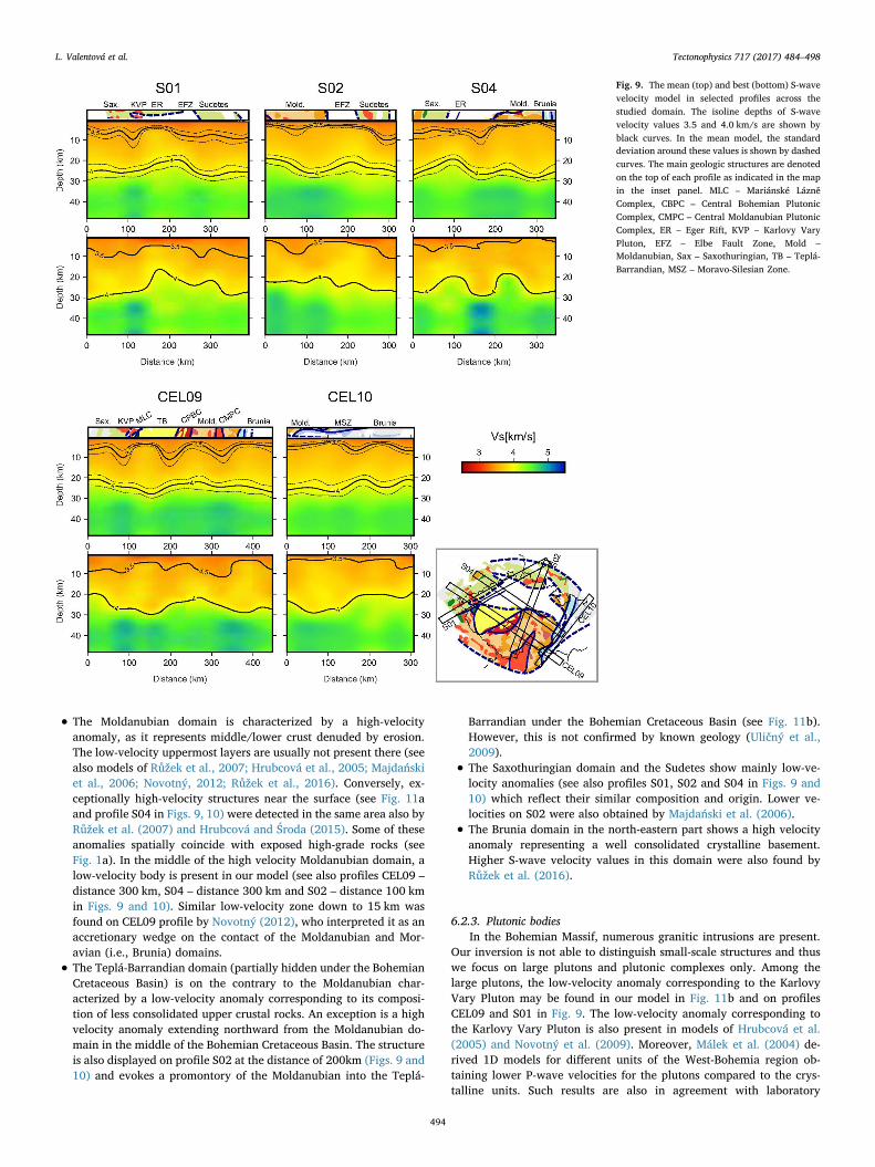
• The Moldanubian domain is characterized by a high-velocityanomaly, as it represents middle/lower crust denuded by erosion.The low-velocity uppermost layers are usually not present there (seealso models of Růžek et al., 2007; Hrubcová et al., 2005; Majdańskiet al., 2006; Novotný, 2012; Růžek et al., 2016). Conversely, ex-ceptionally high-velocity structures near the surface (see Fig. 11aand profile S04 in Figs. 9, 10) were detected in the same area also byRůžek et al. (2007) and Hrubcová and Środa (2015). Some of theseanomalies spatially coincide with exposed high-grade rocks (seeFig. 1a). In the middle of the high velocity Moldanubian domain, alow-velocity body is present in our model (see also profiles CEL09 –distance 300 km, S04 – distance 300 km and S02 – distance 100 kmin Figs. 9 and 10). Similar low-velocity zone down to 15 km wasfound on CEL09 profile by Novotný (2012), who interpreted it as anaccretionary wedge on the contact of the Moldanubian and Mor-avian (i.e., Brunia) domains.

• The Teplá-Barrandian domain (partially hidden under the BohemianCretaceous Basin) is on the contrary to the Moldanubian char-acterized by a low-velocity anomaly corresponding to its composi-tion of less consolidated upper crustal rocks. An exception is a highvelocity anomaly extending northward from the Moldanubian do-main in the middle of the Bohemian Cretaceous Basin. The structureis also displayed on profile S02 at the distance of 200km (Figs. 9 and10) and evokes a promontory of the Moldanubian into the Teplá-

Barrandian under the Bohemian Cretaceous Basin (see Fig. 11b).However, this is not confirmed by known geology (Uličný et al.,2009).

• The Saxothuringian domain and the Sudetes show mainly low-ve-locity anomalies (see also profiles S01, S02 and S04 in Figs. 9 and10) which reflect their similar composition and origin. Lower ve-locities on S02 were also obtained by Majdański et al. (2006).

• The Brunia domain in the north-eastern part shows a high velocityanomaly representing a well consolidated crystalline basement.Higher S-wave velocity values in this domain were also found byRůžek et al. (2016).

6.2.3. Plutonic bodiesIn the Bohemian Massif, numerous granitic intrusions are present.

Our inversion is not able to distinguish small-scale structures and thuswe focus on large plutons and plutonic complexes only. Among thelarge plutons, the low-velocity anomaly corresponding to the KarlovyVary Pluton may be found in our model in Fig. 11b and on profilesCEL09 and S01 in Fig. 9. The low-velocity anomaly corresponding tothe Karlovy Vary Pluton is also present in models of Hrubcová et al.(2005) and Novotný et al. (2009). Moreover, Málek et al. (2004) de-rived 1D models for different units of the West-Bohemia region ob-taining lower P-wave velocities for the plutons compared to the crys-talline units. Such results are also in agreement with laboratory

Fig. 9. The mean (top) and best (bottom) S-wavevelocity model in selected profiles across thestudied domain. The isoline depths of S-wavevelocity values 3.5 and 4.0 km/s are shown byblack curves. In the mean model, the standarddeviation around these values is shown by dashedcurves. The main geologic structures are denotedon the top of each profile as indicated in the mapin the inset panel. MLC – Mariánské LázněComplex, CBPC – Central Bohemian PlutonicComplex, CMPC – Central Moldanubian PlutonicComplex, ER – Eger Rift, KVP – Karlovy VaryPluton, EFZ – Elbe Fault Zone, Mold –Moldanubian, Sax – Saxothuringian, TB – Teplá-Barrandian, MSZ – Moravo-Silesian Zone.

L. Valentová et al. Tectonophysics 717 (2017) 484–498

494

measurements for granitic rocks in this area (see also Pros et al., 1998).Another large plutonic bodies that might be inferred by our inver-

sion are the Central Bohemian Plutonic Complex and the CentralMoldanubian Plutonic Complex. In the vicinity of the Central BohemianPluton a low-velocity anomaly is observed. This anomaly may,

however, belong to the adjacent Teplá-Barrandian domain, where thelower velocities are typical. In the case of the Central MoldanubianPluton, a low-velocity anomaly is present just below its northern tip.However, it does not continue below the southern part of the Pluton,which makes interpretation of this anomaly debatable.

Fig. 10. The S-wave velocity perturbations with respect toaverage model for each depth calculated from the mean modelalong the studied profiles. The main geologic structures aredenoted on the top of each profile as indicated in the map in theinset panel. MLC – Mariánské Lázně Complex, CBPC – CentralBohemian Plutonic Complex, CMPC – Central MoldanubianPlutonic Complex, ER – Eger Rift, KVP – Karlovy Vary Pluton,EFZ – Elbe Fault Zone, Mold – Moldanubian, Sax –Saxothuringian, TB – Teplá-Barrandian, MSZ – Moravo-SilesianZone.

Fig. 11. Topography of the iso-S-wave velocitysurface for value 3.25 km/s and 3.6 km/s of themean model. The main geologic structures areshown (MLC – Mariánské Lázně Complex, CBPC –Central Bohemian Plutonic Complex, CMPC –Central Moldanubian Plutonic Complex, KVP –Karlovy Vary Pluton, FZ – Fault Zone).

L. Valentová et al. Tectonophysics 717 (2017) 484–498

495

All these three anomalies are clearly visible as low-velocity per-turbations in Fig. 10 – profiles CEL09 and S01, where they extend downto ∼20 km depth. For plutonic bodies, such a large depth extent isunlikely as confirmed by other studies: i) gravity modeling by Guy et al.(2011) indicated that the Central Bohemian Plutonic Complex andCentral Moldanubian Plutonic Complex reach to 5 and 10 km, respec-tively, and ii) the Karlovy Vary Pluton was identified as a low velocityanomaly extending down to 10 km on the CEL09 profile by Hrubcováet al. (2005) and Novotný (2012). The supposed overestimation of thedepth extent of these anomalies in our model may be ascribed to thevertical smoothing effect of the surface waves.

6.2.4. Eger RiftThe most distinct structure in our model is in the area of the Eger

Rift: the Saxothuringian – Teplá-Barrandian boundary fault active evennowadays. Under the sediments, the Eger Rift is characterized by a verystrong high-velocity anomaly extending deep in the lower crust (seeFig. 11b; profiles S01 and S04 and the southern rim of the Eger Riftanomaly is also seen at distances 100–150 km of CEL09, Figs. 9 and 10).In this area, higher S-wave velocities down to lower crust were alreadyfound by Kolínský et al. (2011). High P-wave velocities were found byAlexandrakis et al. (2014), Mousavi et al. (2015). The S01 profile ex-tends along the Eger Rift where the high velocity bodies were alreadyfound by Růžek et al. (2007) and by Grad et al. (2008). Grad et al.(2008) interpreted their two separate high-velocity bodies originatingin the lower crust and continuing to the shallower depths as a result ofthe Saxothuringian subduction. The Moho updoming in this area wasfound by Heuer et al. (2006) and in the S04 model of Hrubcová andŚroda (2015). However, our model, despite apparent reversal of theanomaly at greater depths (see bottomost map in Figs. 5 and 6), is lesssensitive to the deep structures and is unable to contradict or confirmthe continuation of the high-velocity anomaly to greater depths.

7. Conclusions

We have inverted ambient noise inter-station dispersion curves intothe 3D S-wave velocity model of the Bohemian Massif. The traditionaltwo-step approach is modified by employing the finite-frequency ad-joint method in the first step, and in the second step by performingBayesian inversion by the parallel tempering algorithm for all modelparameters simultaneously.

For the interpretation, we have considered the mean velocity modeland its uncertainty which were calculated from all resulting 3D modelssampling the posterior PDF (more than 1 million models). The meanmodel reveals the structures that are stable in the inversion. The esti-mated uncertainty helps us to assess reliability of the individual modelfeatures. As the main drawback of our model one may consider its lackof the more detailed structures for the geological interpretations. Inaddition, the surface geology is not perfectly related to the deep crustalstructure that is imaged by surface waves inherently smoothing bothlaterally and vertically the true velocity structure.

The inferred 3D S-wave velocity model shows good correlation withmain geologic domains of the Bohemian Massif. The Moldanubian do-main is characterized by high S-wave velocities representing exposedmiddle/lower crustal material, except for a distinct anomaly located inits central part. Similarly to the Moldanubian, Brunia shows higher S-wave velocity anomalies. In contrast, the Teplá-Barrandian,Saxothuringian and Sudetes domains show lower S-wave velocities. Inthe Teplá-Barrandian domain, we have recovered a high velocity regionwith unclear geological interpretation resembling a promontory of theMoldanubian domain.

The most prominent high-velocity anomaly in the model is foundbeneath the Eger Rift. Moreover, some of the low S-wave velocityanomalies present in our model may correspond to large plutonicbodies, and the topmost low velocity structures correlate well with thesedimentary cover of the Bohemian Massif.

Acknowledgments

We would like to thank two anonymous reviewers for their helpfulcomments to improve the manuscript. This research has been supportedby Charles University grant SVV 260447/2017. We acknowledge fi-nancial support through the GACR (Grantova Agentura CeskeRepubliky) project no. 17-22207S. This work was supported by TheMinistry of Education, Youth and Sports from the Large Infrastructuresfor Research, Experimental Development and Innovations project“IT4Innovations National Supercomputing Center – LM2015070”. Wewould like to express our deepest gratitude to all that provided the data:CRSN network, all BOHEMA and PASSEQ experiments and otherVEBSN stations. We thank Malcolm Sambridge for providing paralleltempering software (available from http://www.iearth.org.au) andOldřich Novotný for VDISP code.

References

Alexandrakis, C., Calò, M., Bouchaala, F., Vavrycuk, V., 2014. Velocity structure and therole of fluids in the West Bohemia Seismic Zone. Solid Earth 5 (2), 863.

Babuška, V., Plomerová, J., 2013. Boundaries of mantle-lithosphere domains in theBohemian Massif as extinct exhumation channels for high-pressure rocks. GondwanaRes. 23 (3), 973–987.

Babuška, V., Plomerová, J., Vecsey, L., Jedlička, P., Růžek, B., 2005. Ongoing passiveseismic experiments unravel deep lithosphere structure of the Bohemian Massif. Stud.Geophys. Geod. 49 (3), 423–430.

Badal, J., Chen, Y., Chourak, M., Stankiewicz, J., 2013. S-wave velocity images of theDead Sea Basin provided by ambient seismic noise. J. Asian Earth Sci. 75, 26–35.

Beard, B.L., Medaris, L.G., Johnson, C.M., Jelínek, E., Tonika, J., Riciputi, L.R., 1995.Geochronology and geochemistry of eclogites from the Mariánské Lázně Complex,Czech Republic: implications for Variscan orogenesis. Geol. Rundsch. 84 (3),552–567.

Behm, M., 2009. 3-D modelling of the crustal S-wave velocity structure from active sourcedata: application to the Eastern Alps and the Bohemian Massif. Geophys. J. Int. 179(1), 265.

Bodin, T., Sambridge, M., Tkalčić, H., Arroucau, P., Gallagher, K., Rawlinson, N., 2012.Transdimensional inversion of receiver functions and surface wave dispersion. J.Geophys. Res. Solid Earth 117 (B2), B02301.

Campillo, M., Paul, A., 2003. Long-range correlations in the diffuse seismic coda. Science299 (5606), 547–549.

Čermák, V., 1994. Results of heat flow studies in Czechoslovakia. In: Bucha, V.,Blížkovský, M. (Eds.), Crustal Structure of the Bohemian Massif and the WestCarpathians. Springer, Berlin, pp. 85–118.

Cho, K.H., Herrmann, R.B., Ammon, C.J., Lee, K., 2007. Imaging the upper crust of theKorean Peninsula by surface-wave tomography. Bull. Seismol. Soc. Am. 97 (1B),198–207.

Cloetingh, S., van Wees, J., Ziegler, P., Lenkey, L., Beekman, F., Tesauro, M., Förster, A.,Norden, B., Kaban, M., Hardebol, N., Bonté, D., Genter, A., Guillou-Frottier, L.,Voorde, M.T., Sokoutis, D., Willingshofer, E., Cornu, T., Worum, G., 2010.Lithosphere tectonics and thermo-mechanical properties: an integrated modellingapproach for enhanced geothermal systems exploration in Europe. Earth-Sci. Rev.102 (34), 159–206.

Czech Regional Seismological Network. https://www.ig.cas.cz/en/structure/observatories/czech-regional-seismological-network.

Dèzes, P., Schmid, S., Ziegler, P., 2004. Evolution of the European Cenozoic Rift System:interaction of the Alpine and Pyrenean orogens with their foreland lithosphere.Tectonophysics 389 (12), 1–33.

Dörr, W., Zulauf, G., 2010. Elevator tectonics and orogenic collapse of a Tibetan-styleplateau in the European Variscides: the role of the Bohemian shear zone. Int. J. EarthSci. 99 (2), 299–325.

Drost, K., Linnemann, U., McNaughton, N., Fatka, O., Kraft, P., Gehmlich, M., Tonk, C.,Marek, J., 2004. New data on the Neoproterozoic-Cambrian geotectonic setting of theTeplá-Barrandian volcano-sedimentary successions: geochemistry, U-Pb zircon ages,and provenance (Bohemian Massif, Czech Republic). Int. J. Earth Sci. 93 (5),742–757.

Fichtner, A., Bunge, H.-P., Igel, H., 2006. The adjoint method in seismology: I. Theory.Phys. Earth Planet. Inter. 157 (1), 86–104.

Finger, F., Gerdes, A., René, M., Riegler, G., 2009. The Saxo-Danubian Granite Belt:magmatic response to post-collisional delamination of mantle lithosphere below thesouthwestern sector of the Bohemian Massif (Variscan orogen). Geol. Carpath. 60 (3),205–212.

Franke, W., 2000. The mid-European segment of the Variscides: tectonostratigraphicunits, terrane boundaries and plate tectonic evolution. Geol. Soc. Lond. Spec. Publ.179 (1), 35–61.

Galetti, E., Curtis, A., Baptie, B., Jenkins, D., Nicolson, H., 2017. Transdimensional Love-wave tomography of the British Isles and shear-velocity structure of the East Irish SeaBasin from ambient-noise interferometry. Geophys. J. Int. 208 (1), 36.

Gao, H., Humphreys, E.D., Yao, H., van der Hilst, R.D., 2011. Crust and lithospherestructure of the northwestern U.S. with ambient noise tomography: terrane accretionand Cascade arc development. Earth Planet. Sci. Lett. 304 (12), 202–211.

L. Valentová et al. Tectonophysics 717 (2017) 484–498

496

Geissler, W.H., Kämpf, H., Kind, R., Bräuer, K., Klinge, K., Plenefisch, T., Horálek, J.,Zedník, J., Nehybka, V., 2005. Seismic structure and location of a CO2 source in theupper mantle of the western Eger (Ohře) Rift, central Europe. Tectonics 24 (5)TC5001.

Geissler, W.H., Kämpf, H., Skácelová, Z., Plomerová, J., Babuška, V., Kind, R., 2012.Lithosphere structure of the NE Bohemian Massif (Sudetes) A teleseismic receiverfunction study. Tectonophysics 564565, 12–37.

Grad, M., Guterch, A., Mazur, S., Keller, G.R., Špičák, A., Hrubcová, P., Geissler, W.H.,2008. Lithospheric structure of the Bohemian Massif and adjacent Variscan belt incentral Europe based on profile S01 from the SUDETES 2003 experiment. J. Geophys.Res. Solid Earth 113 (B10), B10304.

Guo, Z., Chen, Y.J., Ning, J., Feng, Y., Grand, S.P., Niu, F., Kawakatsu, H., Tanaka, S.,Obayashi, M., Ni, J., 2015. High resolution 3-D crustal structure beneath NE Chinafrom joint inversion of ambient noise and receiver functions using NECESSArray data.Earth Planet. Sci. Lett. 416, 1–11.

Guo, Z., Chen, Y.J., Ning, J., Yang, Y., Afonso, J.C., Tang, Y., 2016. Seismic evidence ofon-going sublithosphere upper mantle convection for intra-plate volcanism inNortheast China. Earth Planet. Sci. Lett. 433, 31–43.

Guo, Z., Gao, X., Wang, W., Yao, Z., 2012. Upper- and mid-crustal radial anisotropy be-neath the central Himalaya and southern Tibet from seismic ambient noise tomo-graphy. Geophys. J. Int. 189 (2), 1169–1182.

Guy, A., Edel, J.-B., Schulmann, K., Tomek, Č., Lexa, O., 2011. A geophysical model of theVariscan orogenic root (Bohemian Massif): implications for modern collisional oro-gens. Lithos 124 (12), 144–157.

Haned, A., Stutzmann, E., Schimmel, M., Kiselev, S., Davaille, A., Yelles-Chaouche, A.,2015. Global tomography using seismic hum. Geophys. J. Int. 204 (2), 1222.

Heuer, B., Geissler, W., Kind, R., Kämpf, H., 2006. Seismic evidence for asthenosphericupdoming beneath the western Bohemian Massif, central Europe. Geophys. Res. Lett.33 (5) L05311.

Hrubcová, P., Środa, P., 2015. Complex local Moho topography in the WesternCarpathians: indication of the ALCAPA and the European Plate contact.Tectonophysics 638, 63–81.

Hrubcová, P., Środa, P., Grad, M., Geissler, W., Guterch, A., Vozár, J., Hegedűs, E.,Sudetes 2003 Working Group, 2010. From the Variscan to the Alpine Orogeny:crustal structure of the Bohemian Massif and the Western Carpathians in the light ofthe SUDETES 2003 seismic data. Geophys. J. Int. 183 (2), 611–633.

Hrubcová, P., Środa, P., CELEBRATION 2000 Working Group, et al., 2008. Crustalstructure at the easternmost termination of the Variscan belt based on CELEBRATION2000 and ALP 2002 data. Tectonophysics 460 (1), 55–75.

Hrubcová, P., Środa, P., Špičák, A., Guterch, A., Grad, M., Keller, G., Brueckl, E., Thybo,H., 2005. Crustal and uppermost mantle structure of the Bohemian Massif based onCELEBRATION 2000 data. J. Geophys. Res. Solid Earth 110 (B11), B11305.

Janoušek, V., Bowes, D., Rogers, G., Farrow, C.M., Jelínek, E., 2000. Modelling diverseprocesses in the petrogenesis of a composite batholith: the Central Bohemian Pluton,Central European Hercynides. J. Petrol. 41 (4), 511.

Jiang, C., Yang, Y., Rawlinson, N., Griffin, W.L., 2016. Crustal structure of the NewerVolcanics Province, SE Australia, from ambient noise tomography. Tectonophysics683, 382–392.

Jiang, C., Yang, Y., Zheng, Y., 2014. Penetration of mid-crustal low velocity zone acrossthe Kunlun Fault in the NE Tibetan Plateau revealed by ambient noise tomography.Earth Planet. Sci. Lett. 406, 81–92.

Kalvoda, J., Babek, O., Fatka, O., Leichmann, J., Melichar, R., Nehyba, S., Spacek, P.,2008. Brunovistulian terrane (Bohemian Massif, Central Europe) from lateProterozoic to late Paleozoic: a review. Int. J. Earth Sci. 97 (3), 497–518.

Karousová, H., Plomerová, J., Babuška, V., 2012. Three-dimensional velocity model of thecrust of the Bohemian Massif and its effects on seismic tomography of the uppermantle. Stud. Geophys. Geod. 56 (1), 249–267.

Kolínský, P., Málek, J., Brokešová, J., 2011. Shear wave crustal velocity model of thewestern Bohemian Massif from Love wave phase velocity dispersion. J. Seismol. 15(1), 81–104.

Li, H., Su, W., Wang, C.-Y., Huang, Z., Lv, Z., 2010. Ambient noise Love wave tomographyin the eastern margin of the Tibetan plateau. Tectonophysics 491 (14), 194–204Great 12 May 2008 Wenchuan Earthquake (Mw7.9), China.

Lin, F.-C., Moschetti, M.P., Ritzwoller, M.H., 2008. Surface wave tomography of thewestern United States from ambient seismic noise: Rayleigh and Love wave phasevelocity maps. Geophys. J. Int. 173 (1), 281.

Lin, F.-C., Ritzwoller, M.H., Townend, J., Bannister, S., Savage, M.K., 2007. Ambientnoise Rayleigh wave tomography of New Zealand. Geophys. J. Int. 170 (2), 649.

Luo, Y., Xu, Y., Yang, Y., 2012. Crustal structure beneath the Dabie orogenic belt fromambient noise tomography. Earth Planet. Sci. Lett. 313314, 12–22.

Majdański, M., Grad, M., Guterch, A., SUDETES 2003 Working Group, et al., 2006. 2-Dseismic tomographic and ray tracing modelling of the crustal structure across theSudetes Mountains basing on SUDETES 2003 experiment data. Tectonophysics 413(3), 249–269.

Majdański, M., Kozlovskaya, E., Grad, M., SUDETES 2003 Working Group, 2007. 3Dstructure of the Earth's crust beneath the northern part of the Bohemian Massif.Tectonophysics 437 (14), 17–36.

Málek, J., Janský, J., Novotný, O., Rössler, D., 2004. Vertically inhomogeneous models ofthe upper crustal structure in the West-Bohemian seismoactive region inferred fromthe celebration 2000 refraction data. Stud. Geophys. Geod. 48 (4), 709–730 (Oct).

Matos, C., Silveira, G., Matias, L., Caldeira, R., Ribeiro, M.L., Dias, N.A., Krüger, F., dosSantos, T.B., 2015. Upper crustal structure of Madeira Island revealed from ambientnoise tomography. J. Volcanol. Geotherm. Res. 298, 136–145.

Matte, P., 2001. The Variscan collage and orogeny (480-290 Ma) and the tectonic defi-nition of the Armorica microplate: a review. Terra Nova 13 (2), 122–128.

Mordret, A., Landès, M., Shapiro, N., Singh, S., Roux, P., 2014. Ambient noise surface

wave tomography to determine the shallow shear velocity structure at Valhall: depthinversion with a Neighbourhood Algorithm. Geophys. J. Int. 198 (3), 1514.

Mosegaard, K., Tarantola, A., 1995. Monte Carlo sampling of solutions to inverse pro-blems. J. Geophys. Res. Solid Earth 100 (B7), 12431–12447.

Mousavi, S., Bauer, K., Korn, M., Hejrani, B., 2015. Seismic tomography reveals a mid-crustal intrusive body, fluid pathways and their relation to the earthquake swarms inWest Bohemia/Vogtland. Geophys. J. Int. 203 (2), 1113.

Nicolson, H., Curtis, A., Baptie, B., Galetti, E., 2012. Seismic interferometry and ambientnoise tomography in the British Isles. Proc. Geol. Assoc. 123 (1), 74–86.

Nishida, K., Montagner, J.-P., Kawakatsu, H., 2009. Global surface wave tomographyusing seismic hum. Science 326 (5949) (112–112).

Novotný, M., 2012. Depth-recursive tomography of the Bohemian Massif at the CEL09transect–part B: interpretation. Surv. Geophys. 33 (2), 243–273.

Novotný, M., Skácelová, Z., Mrlina, J., Mlčoch, B., Růžek, B., 2009. Depth-recursive to-mography along the Eger Rift using the S01 profile refraction data: tested at the KTBsuper drilling hole, structural interpretation supported by magnetic, gravity andpetrophysical data. Surv. Geophys. 30 (6), 561 (Nov.).

Novotný, O., Urban, L., 1988. Seismic models of the Bohemian Massif and of some ad-jacent regions derived from deep seismic soundings and surface wave investigations:a review. Induced Seism. Assoc. Phenom. 227–249.

Novotný, O., 1999. Seismic Surface Waves. http://geo.mff.cuni.cz/vyuka/Novotny-SeismicSurfaceWaves-ocr.pdf.

Obermann, A., Lupi, M., Mordret, A., Jakobsdóttir, S.S., Miller, S.A., 2016. 3D-ambientnoise Rayleigh wave tomography of Snæfellsjökull Volcano, Iceland. J. Volcanol.Geotherm. Res. 317, 42–52.

Ouyang, L., Li, H., Lü, Q., Yang, Y., Li, X., Jiang, G., Zhang, G., Shi, D., Zheng, D., Sun, S.,et al., 2014. Crustal and uppermost mantle velocity structure and its relationship withthe formation of ore districts in the Middle-Lower Yangtze River region. Earth Planet.Sci. Lett. 408, 378–389.

Pang, G., Feng, J., Lin, J., 2016. Crust structure beneath Jilin Province and LiaoningProvince in China based on seismic ambient noise tomography. J. Volcanol.Geotherm. Res. 327, 249–256.

Peter, D., Tape, C., Boschi, L., Woodhouse, J.H., 2007. Surface wave tomography: globalmembrane waves and adjoint methods. Geophys. J. Int. 171 (3), 1098.

Peter, D., Komatitsch, D., Luo, Y., Martin, R., Le Goff, N., Casarotti, E., Le Loher, P.,Magnoni, F., Liu, Q., Blitz, C., Nissen-Meyer, T., Basini, P., Tromp, J., 2011. Forwardand adjoint simulations of seismic wave propagation on fully unstructured hexahe-dral meshes. Geophys. J. Int. 186 (2), 721.

Pilia, S., Rawlinson, N., Direen, N., Reading, A., Cayley, R., Pryer, L., Arroucau, P.,Duffett, M., 2015. Linking mainland Australia and Tasmania using ambient seismicnoise tomography: implications for the tectonic evolution of the east Gondwanamargin. Gondwana Res. 28 (3), 1212–1227.

Plomerová, J., Achauer, U., Babuška, V., Granet, M., 2003. BOHEMA 2001-2003: passiveseismic experiment to study lithosphere-asthenosphere system in the western part ofthe Bohemian Massif. Stud. Geophys. Geod. 47 (3), 691–701.

Plomerová, J., Vecsey, L., Babuška, V., Granet, M., Achauer, U., 2005. Passive seismicexperiment mosaic - a pilot study of mantle lithosphere anisotropy of the BohemianMassif. Stud. Geophys. Geod. 49 (4), 541–560.

Plomerová, J., Achauer, U., Babuška, V., Vecsey, L., BOHEMA Working Group, 2007.Upper mantle beneath the Eger Rift (Central Europe): plume or asthenosphere up-welling? Geophys. J. Int. 169 (2), 675–682.

Porritt, R.W., Miller, M.S., O’Driscoll, L.J., Harris, C.W., Roosmawati, N., da Costa, L.T.,2016. Continent-arc collision in the Banda Arc imaged by ambient noise tomography.Earth Planet. Sci. Lett. 449, 246–258.

Pros, Z., Lokajíček, T., Přikryl, R., Špičák, A., Vajdová, V., Klíma, K., 1998. Elasticparameters of West Bohemian Granites under hydrostatic pressure. Pure Appl.Geophys. 151 (2), 631–646 (Mar).

Rawlinson, N., Pilia, S., Young, M., Salmon, M., Yang, Y., 2016. Crust and upper mantlestructure beneath southeast Australia from ambient noise and teleseismic tomo-graphy. Tectonophysics 689, 143–156.

Růžek, B., Hrubcová, P., Novotný, M., Špičák, A., Karousová, O., 2007. Inversion of traveltimes obtained during active seismic refraction experiments CELEBRATION 2000,ALP 2002 and SUDETES 2003. Stud. Geophys. Geod. 51 (1), 141–164.

Růžek, B., Holub, K., Rušajová, J., 2011. Three-dimensional crustal model of the Moravo-Silesian region obtained by seismic tomography. Stud. Geophys. Geod. 55 (1),87–107.

Růžek, B., Plomerová, J., Babuška, V., 2012. Joint inversion of teleseismic P waveformsand surface-wave group velocities from ambient seismic noise in the BohemianMassif. Stud. Geophys. Geod. 56 (1), 107–140.

Růžek, B., Valentová, L., Gallovič, F., 2016. Significance of geological units of theBohemian Massif, Czech Republic, as seen by ambient noise interferometry. PureAppl. Geophys. 173 (5), 1663–1682.

Růžek, B., Horálek, J., 2013. Three-dimensional seismic velocity model of the WestBohemia/Vogtland seismoactive region. Geophys. J. Int. 195 (2), 1251–1266.

Ryberg, T., Muksin, U., Bauer, K., 2016. Ambient seismic noise tomography reveals ahidden caldera and its relation to the Tarutung pull-apart basin at the Sumatran FaultZone, Indonesia. J. Volcanol. Geotherm. Res. 321, 73–84.

Sambridge, M., 2014. A parallel tempering algorithm for probabilistic sampling andmultimodal optimization. Geophys. J. Int. 196 (1), 357.

Saygin, E., Kennett, B.L., 2010. Ambient seismic noise tomography of Australian con-tinent. Tectonophysics 481 (14), 116–125.

Schulmann, K., Konopásek, J., Janoušek, V., Lexa, O., Lardeaux, J.-M., Edel, J.-B., Štípská,P., Ulrich, S., 2009. An Andean type Palaeozoic convergence in the Bohemian Massif.Compt. Rendus Geosci. 341 (23), 266–286.

Schulmann, K., Lexa, O., Janoušek, V., Lardeaux, J.M., Edel, J.B., 2014. Anatomy of adiffuse cryptic suture zone: an example from the Bohemian Massif, European

L. Valentová et al. Tectonophysics 717 (2017) 484–498

497

Variscides. Geology 42 (4), 275–278.Shapiro, N.M., Campillo, M., 2004. Emergence of broadband Rayleigh waves from cor-

relations of the ambient seismic noise. Geophys. Res. Lett. 31 (7), L07614.Shapiro, N.M., Campillo, M., Stehly, L., Ritzwoller, M.H., 2005. High-resolution surface-

wave tomography from ambient seismic noise. Science 307 (5715), 1615–1618.Shen, W., Ritzwoller, M.H., Schulte-Pelkum, V., Lin, F.-C., 2012. Joint inversion of surface

wave dispersion and receiver functions: a Bayesian Monte-Carlo approach. Geophys.J. Int. 192 (2), 807.

Shirzad, T., Shomali, Z.H., 2014. Shallow crustal radial anisotropy beneath the Tehranbasin of Iran from seismic ambient noise tomography. Phys. Earth Planet. Inter. 231,16–29.

Spica, Z., Cruz-Atienza, V.M., Reyes-Alfaro, G., Legrand, D., Iglesias, A., 2014. Crustalimaging of western Michoacán and the Jalisco Block, Mexico, from ambient seismicnoise. J. Volcanol. Geotherm. Res. 289, 193–201.

Spica, Z., Caudron, C., Perton, M., Lecocq, T., Camelbeeck, T., Legrand, D., Piña-Flores, J.,Iglesias, A., Syahbana, D.K., 2015. Velocity models and site effects at Kawah Ijenvolcano and Ijen caldera (Indonesia) determined from ambient noise cross-correla-tions and directional energy density spectral ratios. J. Volcanol. Geotherm. Res. 302,173–189.

Tape, C., Liu, Q., Tromp, J., 2007. Finite-frequency tomography using adjoint methods -methodology and examples using membrane surface waves. Geophys. J. Int. 168 (3),1105–1129.

Tape, C., Liu, Q., Maggi, A., Tromp, J., 2010. Seismic tomography of the southernCalifornia crust based on spectral-element and adjoint methods. Geophys. J. Int. 180(1), 433–462.

Tarantola, A., 2005. Inverse Problem Theory and Methods for Model ParameterEstimation. SIAM.

Tarantola, A., Valette, B., 1982. Inverse problems= quest for information. J. geophys 50(3), 150–170.

Tromp, J., Tape, C., Liu, Q., 2005. Seismic tomography, adjoint methods, time reversaland Banana-Doughnut kernels. Geophys. J. Int. 160 (1), 195–216.

Uličný, D., Špičáková, L., Grygar, R., Svobodová, M., Čech, S., Laurin, J., 2009.Palaeodrainage systems at the basal unconformity of the Bohemian Cretaceous Basin:

roles of inherited fault systems and basement lithology during the onset of basinfilling. Bull. Geosci. 84 (4), 577–610.

Valentová, L., Gallovič, F., Růžek, B., de la Puente, J., Moczo, P., 2015. Choice of reg-ularization in adjoint tomography based on two-dimensional synthetic tests.Geophys. J. Int. 202 (2), 787–799.

Wilde-Piórko, M., Saul, J., Grad, M., 2005. Differences in the crustal and uppermostmantle structure of the Bohemian Massif from teleseismic receiver functions. Stud.Geophys. Geod. 49 (1), 85–107.

Wilde-Piórko, M., Geissler, W., Plomerová, J., Grad, M., Babuška, V., Brückl, E., Cyziene,J., Czuba, W., England, R., Gaczyński, E., Gaždová, R., Gregersen, S., Guterch, A.,Hanka, W., Hegedüs, E., Heuer, B., Jedlička, P., Lazauskiene, J., Keller, G., Kind, R.,Klinge, K., Kolínský, P., Komminaho, K., Kozlovskaya, E., Krüger, F., Larsen, T.,Majdański, M., Málek, J., Motuza, G., Novotný, O., Pietrasiak, R., Plenefisch, T.,Růžek, B., Sliaupa, S., Środa, P., Świeczak, M., Tiira, T., Voss, P., Wiejacz, P., 2008.PASSEQ 2006–2008: passive seismic experiment in trans-European suture zone. Stud.Geophys. Geod. 52 (3), 439–448.

Yang, Y., Ritzwoller, M.H., Levshin, A.L., Shapiro, N.M., 2007. Ambient noise Rayleighwave tomography across Europe. Geophys. J. Int. 168 (1), 259–274.

Yang, Y., Ritzwoller, M.H., Lin, F.-C., Moschetti, M.P., Shapiro, N.M., 2008. Structure ofthe crust and uppermost mantle beneath the western United States revealed by am-bient noise and earthquake tomography. J. Geophys. Res. Solid Earth 113 (B12),B12310.

Young, M.K., Cayley, R.A., McLean, M.A., Rawlinson, N., Arroucau, P., Salmon, M., 2013.Crustal structure of the east Gondwana margin in southeast Australia revealed bytransdimensional ambient seismic noise tomography. Geophys. Res. Lett. 40 (16),4266–4271.

Young, M.K., Rawlinson, N., Bodin, T., 2013. Transdimensional inversion of ambientseismic noise for 3D shear velocity structure of the Tasmanian crust. Geophysics 78(3), WB49–WB62.

Zha, Y., Webb, S.C., Wei, S.S., Wiens, D.A., Blackman, D.K., Menke, W., Dunn, R.A.,Conder, J.A., 2014. Seismological imaging of ridge-arc interaction beneath theEastern Lau Spreading Center from OBS ambient noise tomography. Earth Planet. Sci.Lett. 408, 194–206.

L. Valentová et al. Tectonophysics 717 (2017) 484–498

498