Three-dimensional model for the crust and upper mantle in

the Barents Sea region

H. Bungum1∗, O. Ritzmann2, N. Maercklin1, J.-I. Faleide2, W. D. Mooney3,and S. T. Detweiler3

1NORSAR, Kjeller, Norway; 2University of Oslo, Norway;3U. S. Geological Survey, Menlo Park, California, USA

April 2005

Journal article, originally published as: H. Bungum, O. Ritzmann, N. Maercklin, J.-I. Faleide,W. D. Mooney, and S. T. Detweiler (2005). Three-dimensional model for the crust and uppermantle in the Barents Sea region. EOS Transactions, American Geophysical Union, 86(16), 160–161, doi:10.1029/2005EO160003.

Keywords: seismic velocity model – crust – upper mantle – Barents Sea – European Arctic

Abstract

The Barents Sea and its surroundings is an epicontinental region which previously hasbeen difficult to access, partly because of its remote Arctic location (Figure 1) and partlybecause the region has been politically sensitive. Now, however, this region, and in particularits western parts, has been very well surveyed with a variety of geophysical studies, motivatedin part by exploration for hydrocarbon resources. Since this region is interesting geophysicallyas well as for seismic verification, a major study (Bungum et al., 2004) was initiated in 2003to develop a three-dimensional (3-D) seismic velocity model for the crust and upper mantle,using a grid density of 50 km. This study, in cooperation between NORSAR, the Universityof Oslo (UiO), and the United States Geological Survey (USGS), has led to the constructionof a higher-resolution, regional lithospheric model based on a comprehensive compilation ofavailable seismological and geophysical data. Following the methodology employed in makingthe global crustal model CRUST5.1 (Mooney et al., 1998), the new model consists of fivecrustal layers: soft and hard sediments, and crystalline upper, middle, and lower crust. BothP- and P-wave velocities and densities are specified in each layer. In addition, the densityand seismic velocity structure of the uppermost mantle, essential for Pn and Sn travel timemodeling, are included.

The Barents Sea and its surroundings is an epicontinental region which previously has been difficultto access, partly because of its remote Arctic location (Figure 1) and partly because the regionhas been politically sensitive. Now, however, this region, and in particular its western parts, hasbeen very well surveyed with a variety of geophysical studies, motivated in part by exploration forhydrocarbon resources. Since this region is interesting geophysically as well as for seismic verifi-cation, a major study (Bungum et al., 2004) was initiated in 2003 to develop a three-dimensional(3-D) seismic velocity model for the crust and upper mantle, using a grid density of 50 km.

∗Corresponding author; NORSAR, P.O. Box 53, N-2027 Kjeller, Norway, http://www.norsar.no.

1

Bungum et al. (2005): 3-D model for the Barents Sea region 2

This study, in cooperation between NORSAR, the University of Oslo (UiO), and the United StatesGeological Survey (USGS), has led to the construction of a higher-resolution, regional lithosphericmodel based on a comprehensive compilation of available seismological and geophysical data. Fol-lowing the methodology employed in making the global crustal model CRUST5.1 (Mooney et al.,1998), the new model consists of five crustal layers: soft and hard sediments, and crystalline upper,middle, and lower crust. Both P - and S -wave velocities and densities are specified in each layer.In addition, the density and seismic velocity structure of the uppermost mantle, essential for Pnand Sn travel time modeling, are included.

The general motivation for developing this model is basic geophysical research. A more specificgoal is to create a model for research on the identification and location of small seismic eventsin the study region, and for operational use in locating and characterizing all seismic events inthe region. Along with the development of the model, a calibration and validation program isalso included, aimed at quality controlling the model through comparisons between observed andsynthetic travel times, and at improving regional event locations.

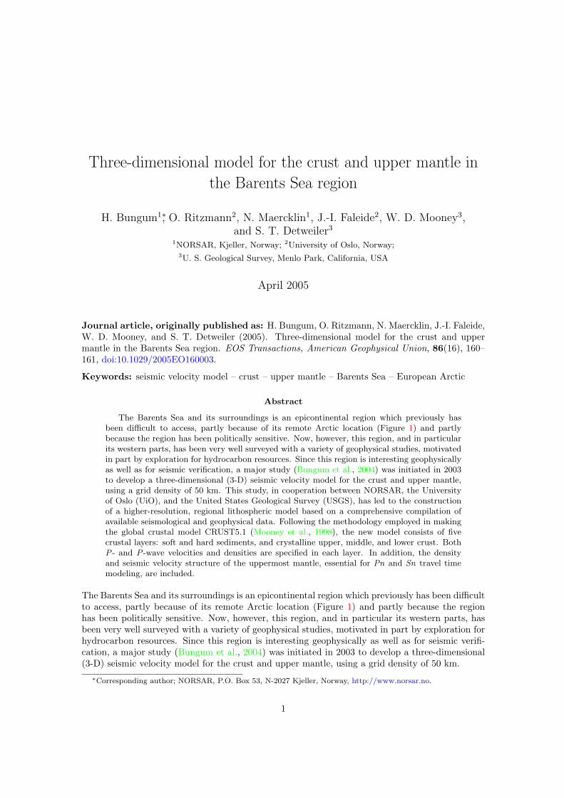
The study area is shown in Figure 1. The principle grid points of the velocity model are shown,with 1490 nodes spaced 50 km apart. The input database consists of 712 1-D velocity-depth profilesthat are based on various kinds of surveys, including onshore and offshore wide-angle experiments,and density modeling along deep seismic reflection profiles with subsequent density-to-velocityconversion. Most of the data sets are published as 2-D crustal velocity cross sections, and thesewere sampled every 25 km to obtain the 1-D velocity-depth profiles.

For each of the grid points in Figure 1, the lithosphere is represented by two sedimentary layersseparated at a P -wave velocity of 3.0 km/s, while the crystalline crust consists of an upper, amiddle, and a lower part that are separated at 6.0 and 6.5 km/s, respectively (6.5 and 7.0 km/sfor oceanic crust). The upper mantle velocity is also specified at each grid point. Values for eachof the tiles located along the wide-angle profiles (Figure 1) are constrained based on primary data.

For regions not constrained by primary data, an interpolation scheme was developed, based onthe definition of geological provinces that are characterized by individual tectono-sedimentaryhistories. Analyses of the compiled database demonstrated strong correlations between sedimentthickness and the thickness of the crystalline basement within each of the continental provinces.Depth-to-basement maps were compiled to use this quantitative correlation as a basis for filling theunconstrained nodes. Within each geological province and each of the crustal layers, the velocitiesare fixed and represented by a mean value calculated from the velocity database. This scheme isvalid for at least 80% of the target region, but is not applicable within the oceanic crustal domain,sediment-free cratons, and regions overprinted by convergent tectonics. For these areas, a simplenearest-neighbor interpolation is applied.

An alternative interpolation approach applies a continuous curvature gridding algorithm for hor-izontal interpolation of seismic velocities within each of the defined provinces. Both of these ap-proaches will be tested in terms of travel time modeling and calibration to explore their potentialsand limitations with respect to seismic velocity model construction.

To provide a complete lithospheric model, the crustal model was complemented with an uppermantle velocity structure based on the work of Shapiro and Ritzwoller (2002), thereby coveringdepths sufficient for the tracing of far-regional wave paths. The final representation of the 3-Dmodel will include depth maps for the interfaces and the lateral velocity variation within eachlayer. For example, the depth to Moho varies from 4 to 5 km (including 2-km water column) offwestern Svalbard (see Figure 1) to 54 km below the northern Scandinavian craton. The P -wavevelocities below the Moho range from 7.4 km/s west of Svalbard to 8.35 km/s below Scandinavia.

Bungum et al. (2005): 3-D model for the Barents Sea region 3

Figure 2 shows an example of a set of geological and geophysical data compiled in this study alongthe 1800-km-long, west-east transect A–A’ in Figure 1. Figure 2a shows a cross section along A–A’and incorporates most of the geophysical data available. The thickness of the sedimentary coverin the Barents/Kara Sea regions may exceed 20 km. Late Permian to Early Triassic convergentmovements along southwestern Novaya Zemlya (the Uralian orogeny, see Figure 1) resulted in upliftand subsequent erosion of sedimentary rocks. Currently, Middle to Late Paleozoic rocks outcropon Novaya Zemlya.

The velocity structure of the crystalline crust and the Moho topography is well known (solidline) from Norwegian and Russian contributions (e.g. Breivik et al., 2003; Sakoulina et al., 2003).Whereas the depth to Moho to the west of the continent-ocean transition (COT) exhibits localvariations, the lower crystalline crust is rather homogeneous with a velocity of 6.8 km/s.

A closer view of the COT along the transect (Figure 2b) (Breivik et al., 2003) presents the detailed2-D seismic velocity structure derived from wide-angle profiles in the target region. Almost everyprofile of the input database is available as a continuous 2-D velocity cross section as is shown here.This was achieved either by obtaining digital models or by digitizing published contour plots. Theinterpretation of seismic velocities was facilitated in particular by deep seismic reflection lines,which are available especially for the western Barents Sea region. Figure 2c shows a data examplewith a prominent crustal root structure (arrows), and Figure 2b a line drawing of the entire line(e.g. Gudlaugsson et al., 1987).

Regional potential-field data taken along transect A–A reveal features that support the geologicalinterpretation (Figure 2d). The comparison of the free-air gravity field with the field calculatedfrom the model will be part of its final validation. Figure 2e shows seismic wave fronts (black,5 s steps) and rays (white) from an initial first arrival travel time modeling using a finite differ-ence method, and Figure 2f compares the corresponding travel time curve (black) with the 1-Dmodels IASPEI91 (blue; Kennett and Engdahl, 1991) and BAREY (red; Schweitzer and Kennett,2002). Reflecting the large lateral inhomogeneities along these profiles, the figure shows significantdeviations from the 1-D travel time models, albeit, as expected, a lot less for the regional model(BAREY) than for the global model (IASPEI91).

Validation of the velocity model includes forward modeling of observed travel times and relocationof seismic events. For this purpose, a set of reference events with known or well-located epicenterswas compiled. Such events are referred to as “Ground Truth” (GT) events. These events aretaken from Hicks et al. (2004) and Bondar et al. (2004), supplemented by additional data fromNORSAR.

The GT events comprise quarry blasts located mainly in Scandinavia and the Kola Peninsula,nuclear explosions in NW Russia and on Novaya Zemlya, and natural earthquakes. With theseevents good travel path coverage is obtained in the western half of the model region and in the SEBarents Sea. The coverage is weaker to the NE, due to a lack of recorded seismicity and man-madeevents from that part of the target region.

This new model of the crust and upper mantle in the greater Barents Sea region is now undergoingfurther refinement and will be completed by the end of 2005. Documentation of the model andinsights into the structure and evolution of the Barents Sea region will be published in forthcomingpapers, and the final model will be made available for use by the scientific community.

Bungum et al. (2005): 3-D model for the Barents Sea region 4

Acknowledgments

We thank Anatoli Levshin for providing the Shapiro and Ritzwoller (2002) mantle velocity model,and William S. Leith and Johannes Schweitzer for their valuable contributions. This researchhas been sponsored by the U.S. Department of Energy under contracts DE-FC52-03NA995081,DE-FC52-03NA995092, and DE-FC52-03NA995313.

References

I. Bondar, E. R. Engdahl, X. Yang, H. A. A. Ghalib, A. Hofstetter, V. Kirichenko, R. Wagner,I. Gupta, G. Ekstrom, E. Bergman, H. Israelsson, and K. McLaughlin (2004). Collection ofa reference event set for regional and teleseismic calibration. Bull. Seism. Soc. Am., 94(4),1528–1545, doi:10.1785/012003128.

A. J. Breivik, R. Mjelde, P. Grogan, H. Shimamura, Y. Murai, and Y. Nishimura (2003). Crustalstructure and transform margin development south of Svalbard on ocean bottom seismometerdata. Tectonophysics, 369, 37–70, doi:10.1016/S0040-1951(03)00131-8.

H. Bungum, O. Ritzmann, J. I. Faleide, N. Maercklin, J. Schweitzer, W. D. Mooney, S. T. Detweiler,and W. S. Leith (2004). Development of a three-dimensional velocity model for the crust andupper mantle in the Barents Sea, Novaya Zemlya and Kola-Karelia regions. In 26th SeismicResearch Review — Trends in nuclear explosion monitoring, pages 50–60, Natl. Nucl. Secur.Admin., Orlando, Florida, 21–23 Sept.

S. T. Gudlaugsson, J. I. Faleide, S. Fanavoll, and B. Johansen (1987). Deep seismic reflec-tion profiles across the western Barents Sea. Geophys. J. R. Astr. Soc., 89(1), 273–278,doi:10.1111/j.1365-246X.1987.tb04419.x.

E. C. Hicks, T. Kværna, S. Mykkeltveit, J. Schweitzer, and F. Ringdal (2004). Travel-times andattenuation relations for regional phases in the Barents Sea region. Pure Appl. Geophys., 161(1), 1–19, doi:10.1007/s00024-003-2437-6.

B. L. N. Kennett and E. R. Engdahl (1991). Travel times for global earthquake location and phaseidentification. Geophys. J. Int., 105(2), 429–465, doi:10.1111/j.1365-246X.1991.tb06724.x.

W. D. Mooney, G. Laske, and T. G. Masters (1998). CRUST 5.1: A global crustal model at 5◦×5◦.J. Geophys. Res., 103(B1), 727–747, doi:10.1029/97JB02122.

T. S. Sakoulina, Y. V. Roslov, and N. M. Ivanova (2003). Deep seismic investigations in the Barentsand Kara seas. Izv. Russ. Acad. Sci. Phys. Solid Earth, 39(6), 438–452.

J. Schweitzer and B. L. N. Kennett (2002). Comparison of location procedures: The Kara Sea eventof 16 August 1997. In F. Ringdal, editor, Semiannual Technical Summary, Scientific Report,1-2002, pages 97–114. NORSAR, Kjeller, Norway.

N. M. Shapiro and M. H. Ritzwoller (2002). Monte-Carlo inversion for a global shear-velocitymodel of the crust and upper mantle. Geophys. J. Int., 151(1), 88–105, doi:10.1046/j.1365-246X.2002.01742.x.

Bungum et al. (2005): 3-D model for the Barents Sea region 5

Figures

Figure 1: Map of the greater Barents Sea region, shown in red in the inset map. The lines markedwith triangles are wide-angle profiles where the color coding indicates the Moho depth. The smallhexagons are tiles spaced 50 km apart that will be filled with crustal and upper mantle velocities.The profile A–A is the one for which detailed results are shown in Figure 2. KFJL, Kaiser FranzJosef Land.

Bungum et al. (2005): 3-D model for the Barents Sea region 6

Figure 2: Observations, interpretations, and modeling for the Barents Sea A–A’ transect shownin Figure 1. Figure 2a shows the geological units along the transect ranging from the oceaniccrustal domain in the very west to Novaya Zemlya and the Kara Sea in the east. Along the1800-km-long transect, all available data were used to display the distribution of sedimentary andcrystalline crustal rocks: 1, Cenozoic sediments; 2, Mesozoic sediments; 3, Paleozoic sediments;4, Paleozoic sediments and/or crystalline rocks; 5, continental crystalline rocks; 6, lower crustalcrystalline rocks with Vp 6.6–6.8 km/s; and 7, oceanic crystalline rocks. Figures 2b and 2c illustratedatabase examples along this transect, i.e., a P-wave velocity model (with line drawing) and deepseismic reflection data, respectively (see insert boxes for along-transect location). Figure 2d showspotential-field data along the profile, Figure 2e shows the 3-D model with superimposed seismicwave fronts, and Figure 2f shows travel times in comparison with two 1-D models. For the velocitymodels in Figures 2b and 2e the lower color scales apply, where the left scale covers the entirerange of lithospheric velocities and the right scale covers the mantle velocities only. Note that at7.8 km/s the scale shows repeating colors (crust-mantle transition).