Seismic imaging of the crust and upper mantle using

Seismic imaging of the crust and upper mantle using regularized

joint receiver functions, frequency––wave number filtering,

and multimode Kirchhoff migration

David Wilson1 and Richard AsterDepartment of Earth and Environmental Science and Geophysical Research Center, New Mexico Institute of Mining andTechnology, Socorro, New Mexico, USA

Received 13 September 2004; revised 3 February 2005; accepted 14 March 2005; published 28 May 2005.

[1] Receiver functions provide an indispensable tool for producing discontinuity imagesof the crust and upper mantle from teleseismic earthquake arrivals. However, imagequality can be significantly compromised by instabilities inherent in the deconvolutionprocess and by irregularities in data coverage driven by source and/or receiver geometries.We present receiver function estimation and prestack migration techniques which bothreduce receiver function deconvolution instability and produce regularized, multimodereceiver function images. The receiver function estimation technique exploits frequency–wave number filtering methods using frequency–pseudowave number domain filtering ofgathers to enhance arrivals with consistent moveout characteristics. Synthetic testsconfirm robust recovery of features in the presence of high noise levels. To processregularized receiver functions into accurate images of the subsurface seismic scatteringpotential, we employ a regularized Kirchhoff migration that migrates both direct andreverberated P-to-S converted modes to their correct subsurface locations. The subsequentimages can be stacked to mute mismigrated modes. Synthetic studies and modelresolution tests demonstrate that this methodology is well suited to irregularly spacedstations and uneven data coverage and does not require the recording of a singleearthquake at multiple stations.

Citation: Wilson, D., and R. Aster (2005), Seismic imaging of the crust and upper mantle using regularized joint receiver functions,

frequency–wave number filtering, and multimode Kirchhoff migration, J. Geophys. Res., 110, B05305,

doi:10.1029/2004JB003430.

1. Introduction

[2] Teleseismic body waves from earthquakes produce aseries of reflections, refractions, and conversions as theytraverse boundaries between regions of differing seismicvelocity and/or impedance. Radial receiver function analy-sis emphasizes P-to-S converted arrivals at these interfacesvia signal deconvolution between horizontal and verticalcomponent seismograms [Langston, 1977; Ammon, 1991;Cassidy, 1992]. In receiver function analysis, the verticalcomponent seismogram of the P wave is characterized as aconvolution of instrument response, vertical site response,and earthquake source function. The radial componentseismogram of the P wave is characterized as the convolu-tion of the instrument response, radial site response, andearthquake source function. Deconvolution of the horizontalsignal by the vertical signal thus removes the commonfactors of instrument response and source function fromthe radial seismogram. The resulting receiver function is

predominantly controlled by the velocity and impedancediscontinuity structure of the upper mantle and crust alongthe ray path, and can be conceptualized as a scaled versionof the radial component of displacement with P multiplesremoved [Ammon, 1991].[3] An inherent problem in calculating receiver functions

is proper regularization of the commonly ill-posed deconvo-lution problem. In this paper we develop receiver functionestimation techniques which take advantage of characteristicmoveout to enhance receiver function arrivals, whileremoving features attributable to noise and deconvolutioninstability.[4] Receiver functions were first applied to solitary

stations to obtain local one-dimensional structure estimates[e.g., Langston, 1977]. Receiver functions at a single stationcan be moveout corrected to a reference epicentral distance,to vertical travel time, or to a common depth axis, andsubsequently stacked to emphasize consistent features. Asthe number of stations available for deep seismic imaginghas increased, receiver function techniques have beenextended to create (to date, frequently two-dimensional)images of fundamental structures such as the Moho or uppermantle transition zone discontinuities [e.g., Sheehan et al.,1995; Yuan et al., 1997; Li et al., 2002]. A commonly usedmethod of producing cross sections referenced to depth

JOURNAL OF GEOPHYSICAL RESEARCH, VOL. 110, B05305, doi:10.1029/2004JB003430, 2005

1Now at Department of Geological Sciences, University of Texas atAustin, Austin, Texas, USA.

Copyright 2005 by the American Geophysical Union.0148-0227/05/2004JB003430$09.00

B05305 1 of 12

from receiver functions is the exploration common conver-sion point (CCP) image [Tessmer and Behle, 1988; Duekerand Sheehan, 1998]. The CCP image is created by firstback projecting the receiver function along a theoretical raypath. The depth cross section is calculated by taking themean sample value (or some other central tendency mea-sure) within bins. Although the CCP method is easilyimplemented and transforms the data into offset and depthspace, it does not correct for diffracted energy or mismap-ped multiples (such as commonly arise from free surfacereverberations).[5] Migration seeks to map seismic energy to its

true subsurface origin (either in time or in depth) whilecollapsing diffraction artifacts, and is necessary to producestructural images that properly correct for wave propagationeffects due to lateral heterogeneity [e.g., Abers, 1998; Eatonet al., 2002]. Recent efforts have included the application ofseismic data migration techniques to teleseismic wavefields, including both prestack [Sheehan et al., 2000;Poppeliers and Pavlis, 2003; Wilson et al., 2003, 2005]and poststack [Ryberg and Weber, 2000] methodologies.Other promising methodologies implement prestackmigration and scattering inversion of the three-componentteleseismic wave field [e.g., Bostock and Rondenay, 1999;Bostock et al., 2001; Fan et al., 2003; Shragge and Artman,2003].[6] Here we present a method of receiver function

migration that uses information contained in both directand reverberated P-to-S converted energy while suppressingreverberation artifacts. The migrated image is constructedusing receiver functions calculated independently at eachstation, making it unnecessary to simultaneously recorda given earthquake teleseismic wave field at multiplestations. Migration with receiver functions rather than thethree-component wave field has the practical advantage ofreducing a vector imaging problem to a scalar imagingproblem [e.g., Levander, 2003]. Receiver function migra-tion produces images of the subsurface P-to-S scatteringpotential [Poppeliers and Pavlis, 2003] as estimated inreceiver function amplitudes. Receiver function amplitudesare, in turn, determined by the amplitude of shear wavearrivals on the radial component scaled by the P wavearrival on the vertical component [Ammon, 1991; Cassidy,1992] and thus contain information about the relative Swave and P wave transmission and reflection coefficientswhich are directly tied to subsurface velocity and imped-ance contrasts. In particular, forward scattering of theincoming wave field (direct converted P-to-S energy) ismost sensitive to contrasts in velocity, while back scatteredphases (reverberated receiver function phases) are mostsensitive to P and S impedance contrasts [Wu and Aki,1985]. We present a receiver function migration methodol-ogy based on regularized Kirchhoff methodology [e.g.,Duquet et al., 2000; Nemeth et al., 1999] that has beenshown to produce subsurface images with higher resolutionand fewer migration artifacts and acquisition geometryartifacts than standard migration algorithms. We developand apply this technique to synthetic receiver functions todemonstrate the benefits for common recording geometrieswhere imaging can be degraded by irregular station spacingand uneven data coverage. These receiver function estima-tion and migration methods are subsequently applied to data

from the RISTRA experiment in the southwestern UnitedStates by Wilson et al. [2005].

2. Receiver Function Estimation

[7] In receiver function modeling incorporating planewaves and flat-lying interfaces, four dominant converted/refracted propagation modes are commonly observed(Figure 1a):[8] 1. The direct P mode, observed as a prominent pulse

near zero time. The deconvolution process should place thispulse exactly at zero time, however shallow structure such assedimentary layers can cause a slight delay (typically less than1 s) and adecrease indirectPpulse amplitude [Cassidy, 1992].[9] 2. Direct P-to-S (Ps) modes generated at each discon-

tinuity. In a flat-layered velocity structure, the arrival timefor the Ps mode relative to the direct P arrival is

TPs ¼ Ts � Tp ð1Þ

where

Ts ¼ H V�2s � p2

� �1=2; Tp ¼ H V�2

p � p2� �1=2

ð2Þ

H is the depth to the converting interface, Vp and Vs are thereciprocal average P and S wave slownesses to theconverting interface, and p is the horizontal slowness (rayparameter) of the teleseismic event. For conversions fromcontinental Moho, the Ps mode typically arrives at an arrivaltime around 4–6 s.[10] 3. The PpPs mode resulting from incoming P

refracting as P at a discontinuity, reflecting downward asP off the free surface, then converting/reflecting upward asS at each discontinuity. The travel time for this arrival is

TPpPs ¼ Ts þ Tp ð3Þ

and typically occurs around 15–20 s for the Moho.[11] 4. The (simultaneously arriving for a flat structure)

PpSs and PsPs arrivals resulting from incoming P, refracting/converting as P or S at a discontinuity, reflecting downwardoff the Earth’s free surface as P or S, and finally reflectingupward as S at each discontinuity. The travel time for thismode is

T PpSsþPsPsð Þ ¼ 2Ts ð4Þ

and is typically observed several seconds after the PpPsMoho arrival. Although PpSs + PsPs energy propagatesalong two simultaneously arriving ray paths for flat-lyinggeometries, in laterally heterogeneous situations the twomodes will not be simultaneous, resulting in destructiveinterference and/or produce a multiple arrival.[12] Receiver function deconvolution may be performed

either in the time [e.g., Sheehan et al., 1995; Zandt andAmmon, 1995; Poppeliers and Pavlis, 2003] or frequencydomains [e.g., Ammon, 1991; Cassidy, 1992; Dueker andSheehan, 1998; Park and Levin, 2000]. In either strategy, aninherent problem is regularizing of the commonly ill-poseddeconvolution [e.g., Aster et al., 2004], where substantialartifacts may be introduced by high noise levels and/or

B05305 WILSON AND ASTER: RECEIVER FUNCTION FILTERING AND MIGRATION

2 of 12

B05305

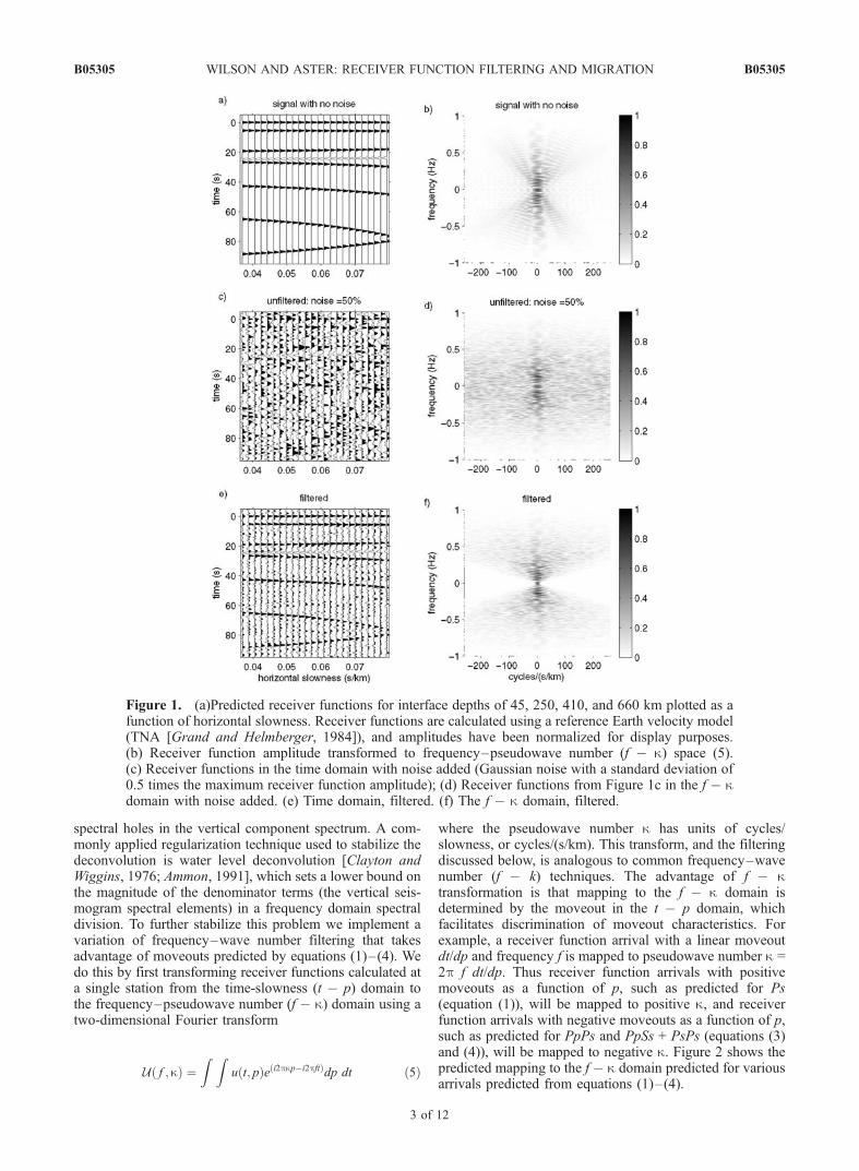
spectral holes in the vertical component spectrum. A com-monly applied regularization technique used to stabilize thedeconvolution is water level deconvolution [Clayton andWiggins, 1976; Ammon, 1991], which sets a lower bound onthe magnitude of the denominator terms (the vertical seis-mogram spectral elements) in a frequency domain spectraldivision. To further stabilize this problem we implement avariation of frequency–wave number filtering that takesadvantage of moveouts predicted by equations (1)–(4). Wedo this by first transforming receiver functions calculated ata single station from the time-slowness (t � p) domain tothe frequency–pseudowave number (f � k) domain using atwo-dimensional Fourier transform

U f ; kð Þ ¼Z Z

u t; pð Þe i2pkp�i2pftð Þdp dt ð5Þ

where the pseudowave number k has units of cycles/slowness, or cycles/(s/km). This transform, and the filteringdiscussed below, is analogous to common frequency–wavenumber (f � k) techniques. The advantage of f � ktransformation is that mapping to the f � k domain isdetermined by the moveout in the t � p domain, whichfacilitates discrimination of moveout characteristics. Forexample, a receiver function arrival with a linear moveoutdt/dp and frequency f is mapped to pseudowave number k =2p f dt/dp. Thus receiver function arrivals with positivemoveouts as a function of p, such as predicted for Ps(equation (1)), will be mapped to positive k, and receiverfunction arrivals with negative moveouts as a function of p,such as predicted for PpPs and PpSs + PsPs (equations (3)and (4)), will be mapped to negative k. Figure 2 shows thepredicted mapping to the f � k domain predicted for variousarrivals predicted from equations (1)–(4).

Figure 1. (a)Predicted receiver functions for interface depths of 45, 250, 410, and 660 km plotted as afunction of horizontal slowness. Receiver functions are calculated using a reference Earth velocity model(TNA [Grand and Helmberger, 1984]), and amplitudes have been normalized for display purposes.(b) Receiver function amplitude transformed to frequency–pseudowave number (f � k) space (5).(c) Receiver functions in the time domain with noise added (Gaussian noise with a standard deviation of0.5 times the maximum receiver function amplitude); (d) Receiver functions from Figure 1c in the f � kdomain with noise added. (e) Time domain, filtered. (f) The f � k domain, filtered.


3 of 12

B05305

[13] Receiver function amplitudes that have large vari-ability as a function of p will map to high k values in the f �k domain at a given frequency. This could occur due toeither high-moveout arrivals (large dt/dp), or to receiverfunction features that do not appear on adjacent receiverfunctions (and may in fact be caused by high backgroundnoise amplified by the instability of the receiver functiondeconvolution). By calculating the maximum predicted dt/dp from (1)–(4) we can calculate the maximum physicallyreasonable range of k and design an f � k filter to attenuatereceiver function amplitudes with high variability as afunction of horizontal slowness while preserving arrivalswith consistent moveout characteristics.[14] The f � k domain filtering of receiver function

amplitudes is accomplished by multiplication by a Gaussianfilter response

F f ; kð Þ ¼ e� 2pkð Þ2= 4b2a2ð Þ ð6Þ

where a = 2pf max (dt/dp). In this study we use a scalingfactor of b = 3.75, which results in approximate filteramplitudes of 0.1 when k = 1.88 � 2pf max (dt/dp),0.5 when k = 2pf max (dt/dp), and 0.9 when k = 0.375 �2pf max (dt/dp). We use a broad Gaussian filter rather anarrower realization targeted at specific arrivals to allowcurvature in predicted moveout times due to dipping orlaterally heterogeneous velocity geometries. The filterapplies the strongest attenuation to receiver functionamplitudes that do not vary smoothly as a function of p,such as would be produced by uncorrelated noise.[15] Figure 1 illustrates the filtering process. Figure 1a

shows receiver function amplitudes in t � p domain aspredicted by equations (1)–(4) using the TNA referenceEarth velocity model [Grand and Helmberger, 1984], andFigure 1b shows the same receiver function amplitudestransformed to the f � k domain. For demonstrationpurposes, receiver function arrival amplitudes at all depthshave been normalized. In Figures 1c and 1d we add whiteuncorrelated Gaussian noise with a standard deviation of

0.5 times the maximum receiver function amplitude. Theadded white noise makes it difficult to discern the lateralcoherency of many of the receiver function arrivals(Figure 1c), and disrupts amplitudes throughout the f � kplane (Figure 1d).[16] We design a filter using (6) by calculating the

maximum predicted dt/dp from (1)–(4) using the TNAreference Earth velocity model. The maximum time move-out, (dt/dp) = 520 s/(s/km) for the predominant phasesoccurs for the Ps arrival from the 660 km upper mantlediscontinuity. Resulting filtered receiver function arrivalsare shown in Figures 1e and 1f in the t � p and f � kdomains, respectively. Improvement is clear in the t � pdomain, with a significant increase in the lateral coherencyof receiver function arrivals. The correlation coefficientbetween Figure 1a and 1c is 0.39, and the correlationcoefficient between Figure 1a and 1e is 0.76.

3. Receiver Function Imaging

3.1. Migration

[17] We next present a method of receiver functionmigration for both direct and reverberated P-to-S convertedarrivals. We cast the problem as a Kirchhoff-style prestackmigration [Yilmaz, 1987; Dellinger et al., 2000] by charac-terizing the model space as a grid of point scatterers. Foreach station we ray trace recorded receiver function arrivals(direct converted, as well as reverberated) to all possiblescattering points within the model space. Receiver functionamplitudes are scaled and summed onto an output migrationgrid according to the Kirchhoff integral, which relates thewave field measured at the surface to the wave field at depth.The far-field term of the (single-component) Kirchhoffintegral can be expressed as [Yilmaz, 1987]

uout x; zð Þ ¼ 1

2p

ZStr

cos qvr

@

@tuin xin; z ¼ 0; tð Þdx ð7Þ

where v is the RMS velocity at the imaging point (x, z), ris the distance between the input (xin, z = 0) and the output(x, z) imaging points, and the time t is the sum of the source-to-imaging point and imaging point-to-receiver travel times.The obliquity factor cos q arises from recording geometry(Figure 3). For vertical component P wave migration, q isthe incidence angle of the ray being imaged, since P waveswill have maximum amplitude on vertical components fornear vertical arrivals. Similarly, for radial receiver functionmigration, q is also the incidence angle of the ray being

Figure 2. Predicted mapping to f � k space of receiverfunction arrivals.

Figure 3. Ray paths for the (a) Ps, (b) PpPs, and (c) PpSsarrivals used for calculating migration travel times andscaling. Point diffractor scattering radiation patterns [e.g.,Wu and Aki, 1985] are indicated at the point scatterers.


4 of 12

B05305

imaged, since a shear wave arrival will have maximumamplitude on horizontal components for near verticalarrivals. The scaling term Str corrects for S wave pointscattering patterns [Wu and Aki, 1985; Levander, 2003](Figure 3) for forward P-to-S scattering or back scattered P-to-S or S-to-S phases, depending on which phase is beingmigrated. For the Ps and PpPs phases (Figures 3a and 3b),Str varies as a function of the sine of the angle between thedirection of scattering and the P wave propagation direction.For PpSs phase (Figure 3c), Str varies as a function of thecosine of the angle between the direction of scatteringand the S wave propagation direction. The factor (vr)�1

reflects spherical spreading and the time derivative providesthe phase shift required by Huygens’ principle [Yilmaz,1987]. In two dimensions the half-order derivative (multi-plication by ({w)1/2 in the frequency domain) is used.[18] Figure 4 illustrates receiver function migration

applied to a lithosphere-scale model featuring a pointscatterer at 50 km depth. Figures 4a and 4b show syntheticvertical and horizontal-radial seismograms, respectively,containing characteristic teleseismic spectral energybetween 15 s and 2 Hz. Figure 4c shows correspondingreceiver functions calculated from Figures 4a and 4b. Notethat the phase associated with the incoming P wave field isnow aligned at time zero by the receiver function deconvo-

lution. Diffractions resulting from the point scatterer canbe seen for the Ps, PpPs, and PpSs phases between 5 and45 s. Figures 4d, 4e, and 4f shows migrations using Ps,PpPs, and PpSs ray path geometries, respectively, using (7).[19] Seismic data migration can be analyzed as an inverse

problem by considering a forward operator G, that maps thevelocity discontinuity structure of the subsurface, m, ontodata, d. For linear situations, this gives the relationship d =Gm. In the context of this paper, an appropriate G may beconstructed using the travel time and scaling relationshipsspecified by (7). For Kirchhoff migration, the inverseoperator that maps data back to the model estimate is GT

[Nemeth et al., 1999]. Regularized migration [e.g., Duquetet al., 2000; Nemeth et al., 1999] applies a generalized andregularized inverse operator, G�g to produce a solution m =G�gd, and has been shown to produce subsurface imageswith higher resolution and fewer migration artifacts andacquisition geometry artifacts than standard migration algo-rithms [Duquet et al., 2000; Nemeth et al., 1999]. However,it is not routinely used in the exploration industry (wherelarge surveys often have over 106 data traces) due to thecomputing power needed to compute and implement G�g.However, passive teleseismic experiments to date such asRISTRA [Wilson et al., 2002, 2003, 2005]) have on theorder of 103 to 104 traces, making such inversion method-

Figure 4. Application of receiver function migration to simulated diffractions from a single pointscatterer. (a), (b), and (c) Vertical component, horizontal radial component, and receiver functions,respectively, for an evenly spaced (10 km) recording network. The point diffractor is located at 50 kmdepth and at 150 km on the horizontal axis. (d), (e), and (f) Ps, PpPs, and PpSs migrated receiverfunctions, respectively.


5 of 12

B05305

ologies far more tractable. Setting up migration as aninverse problem allows for the use of diverse regularizationtechniques. One method is to minimize the Tikhonovobjective function [Aster et al., 2004; Nemeth et al., 1999]

p mð Þ ¼k Gm� d k2 þ� k Cm k2 ð8Þ

The first term in (8) is the 2-norm data misfit and the secondterm is a regularization term scaled by a regularizationparameter, �. C is a conditioning matrix used to penalizeundesirable model properties. We implement a second-orderTikhonov regularization so that left multiplication of themodel by C approximates the second-order spatial deriva-tive. To determine the appropriate �, we compute thesolution to (8) for a range of values of �, and then constructa tradeoff curve between model misfit (kGm � dk2) androughness (kCmk2). We employ a conjugate gradientiterative scheme [e.g., Aster et al., 2004; Rowe et al.,2002] to solve the system for the large, sparse G matrixarising in this application. Travel times relative to P for each

arrival of interest (Figure 3), are calculated for each seismicstation.[20] The travel time for Ps is

tPs ¼ tmod�sta � Tp þ tsrc�Xp� tsrc�sta

� �ð9Þ

where tmod�sta is the travel time from the model point to thestation, Tp is given by (2), tsrc�Xp is the travel time from theepicenter to the point Xp (Figure 3), and tsrc�sta is the traveltime from the epicenter to the recording station. If weassume a flat-layered velocity geometry, we can calculatethe quantity (tsrc�Xp � tsrc�sta) directly from the horizontalslowness without actually calculating the travel time fromthe epicenter. For real data, we need to account for thecurvature and velocity structure of the Earth. In this case,we can calculate the quantity (tsrc�Xp � tsrc�sta) based ontravel times predicted for a reference Earth model as afunction of epicentral distance. Because rays traveling fromthe epicenter to Xp, and from the epicenter to the recordingstation, have taken nearly the same path, the quantity(tsrc�Xp � tsrc�sta) is primarily a function of the distancebetween Xp and the station, and of the horizontal slownessat Xp and the station. Synthetic testing demonstrates that thefine details of the reference Earth velocity model do nothave a large effect. Similarly, for the PpPs migration, thetravel time is

tPpPs ¼ tmod�sta þ Tp þ tsrc�Xp� tsrc�sta

� �ð10Þ

and for the PpSs + PsPs migration it is

tPpSsþPsPs ¼ tmod�sta þ Ts þ tsrc�Xs� tsrc�stað Þ ð11Þ

where tsrc�Xsis the travel time from the epicenter to point Xs

(Figure 3), and Ts is given by (2).[21] Figures 5b, 5c, and 6 show migrated cross sections

for noise-free synthetic receiver function data containing10 stations with a spacing of 40 km and a standard deviationof 20 km. Each station is associated with four receiverfunctions with random back azimuths that are in line withthe imaging plane (i.e., ±180�), and random epicentraldistances between 35� and 95� (corresponding to a rangein values of horizontal slowness, p, between 0.039 and0.078 s/km). Synthetic receiver functions were calculatedfor a 45 km thick crust over a half-space. Ray paths for thesynthetic receiver function data set are shown in Figure 5a.For this synthetic migration example, we have chosen thissimple velocity model in order to emphasize the benefits ofapplying regularized migration to a data set with irregularstation spacing and sparse data coverage. Figures 5b, 6a,and 6c show Kirchhoff migrated cross sections (m = GTd)of the Ps, PpPs, and PpSs + PsPs modes, and thecorresponding regularized migration cross sections areshown in Figures 5c, 6b, and 6d. For each mode theregularized migration shows improved lateral coherencyof imaged receiver function amplitudes. In areas wherethere is a large gap between adjacent stations, the regular-ized migration implements a consistent interpolation toproduce a more spatially continuous image while fittingthe data. The regularized migration also shows a reductionin migration artifacts (‘‘smiles’’) caused by the sparse data

Figure 5. (a) Ray paths for the synthetic receiver functiondata set used for migration demonstration. (b) Kirchhoff-migrated cross sections for the Ps mode and (c) thecorresponding regularized migrated cross sections. Grayscale indicates scattering potential.


6 of 12

B05305

coverage, which are most evident in the Ps migration(Figure 5b). It is important to note that the regularizedmigration does not simply smooth the data, but ratherdetermines a ‘‘best’’ tradeoff between fitting the data andsmoothing the model. The objective function curves for thePs, PpPs, and PpSs + PsPs mode regularized migrationsare shown in Figure 7. The optimal value of � for eachcurve was selected by finding the corner, or ‘‘knee’’, ofthe trade-off curve using the MATLAB function l-corner[Hansen, 1994].

[22] The depth to which each of the receiver functionmodes are migrated depends on the velocity model.However, because each mode has differing sensitivity tovelocity model errors we can use any such systematicinconsistencies to assess the velocity model accuracy.Figure 8 shows the Moho imaging depth error for each ofthe receiver function modes as a function of errors in thevelocity model, calculated from (1)–(4) for the simplesynthetic model with a 45 km thick crust. We find thatthe inferred Moho depth in the migrated images is least

Figure 6. Kirchhoff-migrated cross sections for the (a) PpPs and (c) PpSs + PsPs modes and (b) and(d) the corresponding regularized migrated cross sections. Gray scale is the same as that given in Figure 5.

Figure 7. Objective function curve for the (a) Ps, (b) PpPs, and (c) PpSs + PsPs synthetic migrations.Each data point on the curve represents a solution to (8) for a different value of �. The optimal value of �is selected by finding the corner, or ‘‘knee’’ of the curve [Hansen, 1994].


7 of 12

B05305

sensitive to the starting P wave velocity model. In this case,a 5% over/underestimation of VP shifts each modes imagesof the Moho approximately uniformly 2–2.5 km deeper/shallower. Errors in the VP/VS ratio can have more signif-icant effects, and do not affect all modes in a uniformfashion. For this simple model, a 5% overestimate of the VP/VS ratio results in underestimating the Moho depth from thePs, PpPs, and PpSs + PsPs modes by 4.5, 1.5, and 2.3 km,respectively. A 5% underestimate of VP/VS results in over-estimating the Moho depth from the Ps, PpPs, and PpSs +PsPs modes by 6.0, 1.5, and 2.5 km, respectively.

3.2. Stacking Multiple Migrated Images

[23] Sharp velocity contrasts at the Moho and deepsedimentary basins introduce large amplitude multiples intothe images that produce imaging artifacts and can overprintdeeper structure when migrated. To reduce imaging artifactsthe three migrated output grids are stacked so that largeamplitudes in the final image are produced only when thePs, PpPs, and the negative (due to reflection polarityreversal) of the PpSs + PsPs migration images haveidentical polarity. To emphasize common polarity andamplitude images, we thus employ a multi-image nonlinearstacking algorithm [e.g., Kanasewich et al., 1973] of theform

s ¼ abn ð12Þ

where

a ¼3 median mPs þ mPpPs � mPpSsþPsPs

� �� mPsj j þ mPpPs

�� þ mPpSsþPsPs

�� ð13Þ

b ¼mPs þ mPpPs � mPpSsþPsPs

�� mPsj j þ mPpPs

�� þ mPpSsþPsPs

�� ; ð14Þ

and mPs, mPpPs, and mPpSs+PsPs are the results of the Ps,PpPs, and PpSs + PsPs migrations, respectively. The afactor is a measure of the relative amplitude of the threeimages, and will be maximized when the three images havethe same polarity and amplitude. The bn factor isexclusively a nonlinear measure of polarity consistence. Inregions where all three images have consistent polarity, bn

will have a (maximum) value of 1. The parameter n controlsthe degree of nonlinear scaling applied to the summedimages. As n ! 1, the summed images are multiplied by 1where they all have the same polarity, and multiplied by 0where they do not. The choice of n will depend on thecharacteristics of a particular data set. In this case, we chosea value of n = 8, so that when b has the value of 0.75, bn willequal 0.1.[24] Figure 9 provides a simple illustration of the multi-

mode stacking process using a single receiver functionrecorded at a single station, where the velocity modelconsists of a 45 km thick crust and a horizontal slownessof 0.05 s/km. The first three panels show the depth-mappedreceiver functions for Ps, PpPs, and PpSs + PsPs, respec-tively, and the fourth panel shows the nonlinear stack. Eachof the three single-mode depth-converted traces shows apositive amplitude at the Moho depth of 45 km whichproduces a positive stack trace. Imaging artifacts present inthe single-mode images are severely downweighted by thestacking algorithm. Figure 10 shows the multimode, stackedimages computed from the Kirchhoff-migrated and regular-ized-migrated single-mode images of Figures 5 and 6.Energy from receiver function multiples (e.g., from PpPsand PpSs + PsPs) which migrated to incorrect depths (e.g.,125–200 km) in the Ps migration (Figures 5b and 5c) aswell as energy which was incorrectly migrated by modemisattribution in the PpPs and PpSs + PsPs migrations(Figure 6) has been essentially removed by the stacking

Figure 8. Imaging Moho depth error as a function of velocity errors.


8 of 12

B05305

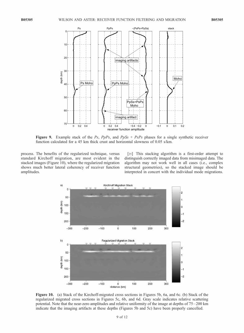
process. The benefits of the regularized technique, versusstandard Kirchoff migration, are most evident in thestacked images (Figure 10), where the regularized migrationshows much better lateral coherency of receiver functionamplitudes.

[25] This stacking algorithm is a first-order attempt todistinguish correctly imaged data from misimaged data. Thealgorithm may not work well in all cases (i.e., complexstructural geometries), so the stacked image should beinterpreted in concert with the individual mode migrations.

Figure 9. Example stack of the Ps, PpPs, and PpSs + PsPs phases for a single synthetic receiverfunction calculated for a 45 km thick crust and horizontal slowness of 0.05 s/km.

Figure 10. (a) Stack of the Kirchoff-migrated cross sections in Figures 5b, 6a, and 6c. (b) Stack of theregularized migrated cross sections in Figures 5c, 6b, and 6d. Gray scale indicates relative scatteringpotential. Note that the near-zero amplitudes and relative uniformity of the image at depths of 75–200 kmindicate that the imaging artifacts at these depths (Figures 5b and 5c) have been properly cancelled.


9 of 12

B05305

One such case is the presence of higher-order multiples,sometimes referred to as ‘‘signal-generated noise’’ [e.g.,Park and Levin, 2000], from near strong near-surface low-velocity zones such as sedimentary basins. If an accuratevelocity model is used, the first-order multiples will stackdestructively, but the higher-order multiples will not, result-ing in imaging artifacts. However, higher-order multipleswill have considerably lower amplitude than the primaryphases and first-order multiples, so that associated imagingartifacts will typically be low in amplitude.

3.3. Migration Resolution

[26] For imaging at crustal levels (e.g., up to approxi-mately 60 km depth) the direct converted phase (Ps) for thebasins and Moho, as well as basin multiples, typically havemaximum energy at approximately 0.5–2 Hz, while thecrustal multiples have most of their energy at 0.15–0.5 Hz.At Moho depths, this translates to about 2 to 6 km verticalresolution (1/2 P wavelength [Bostock, 1999]) for the Psphase, and 4 km vertical resolution for the crustal multiples(1/4 wavelength). Fresnel zone widths at Moho depths areapproximately 8 km at 1 Hz, and 18 km at 4 s periods.However, if we assume that the migration has properlycollapsed diffracted energy, the horizontal resolution aftermigration is improved to approximately 1 wavelength [Stolt

and Benson, 1986], or to about 4 km horizontal resolution at1 Hz and 15 km horizontal resolution at 4 s periods.[27] The resolution of stacked migrated images will

depend on station spacing, data coverage, and inversemethodology (e.g., the choice of the regularization param-eter � in [8]). We assess the resolution of the migrationprocess in a standard ‘‘checkerboard test’’ manner byconsidering a synthetic scattering potential Earth model,mtrue, and a corresponding data set, d = Gmtrue. Applyinga linear generalized inverse operator G�g results in anestimated model

m ¼ G�gd ð15Þ

which can be compared to mtrue to assess the recovery ofmodel and, conversely, the details and the presence ofsmoothing or other artifacts resulting from regularization.Further image degradation may also come about due tonoise, and these influences can be assessed by the additionof noise to the synthetic data. This analysis is analogous toresolution tests commonly performed in tomographicinversions, and assesses bias introduced by regularizationand/or rank deficiency into the linear inverse problem for ageneral weakly scattering Earth structure (which is a solelyfunction of station spacing and data coverage [Aster et al.,

Figure 11. Ps migration resolution test consisting of (a) the scattering potential Earth model used forforward modeling, (b) the corresponding Kirchhoff-migrated cross section, and (c) the regularizedmigrated cross section. Gray scale indicates scattering potential.


10 of 12

B05305

2004]). However, note that this resolution analysis method-ology is not an assessment of the ability of the migration toproperly image the subsurface using the complex, multiplyscattered wave field that would be produced by an actual‘‘checkerboard’’ earth.[28] Figures 11 and 12 show forward modeled resolution

for the station spacing and data coverage used in thesynthetic data migration of Figures 5 and 6. The scatteringpotential Earth model used for forward modeling is shownin Figure 11a and corresponding Kirchhoff-migrated andregularized migrated cross sections are shown in Figures 11band 11c, respectively, for the Ps migration and inFigures 12a and 12c and Figures 12b and 12d, respectively,for the migration of reverberated phases. The Kirchhoff-migrated images (Figures 11b, 12a, and 12c) exhibit con-siderable amplitude variation, with the highest amplitudesoccurring at shallow levels in regions with close station

spacing. Regularized migration (Figures 11c, 12b, and 12d)produces an image with less variation in amplitude, moreclosely resembling the starting model (note the differingcolor scales between the Kirchhoff and regularized migra-tions), and does not show strong amplitude variationsattributable to the irregular station spacing. The effect ofregularization is also evident, giving the regularized migra-tions a smoother appearance than the relatively grainyKirchhoff migrations. Both the Kirchhoff and regularizedmigrated images show that migration resolution degradesrapidly off the ends of the network but the recovery near theedges is improved by the regularized algorithm.

4. Conclusions

[29] Instability in receiver functions produced either byhigh background noise or by holes in the vertical compo-

Figure 12. Migration resolution tests for the PpPs and PpSs+PsPs phases consisting of (a), (c) theKirchhoff-migrated cross sections, and (b), (d) the corresponding regularized migrated cross sections.Gray scale indicates scattering potential.


11 of 12

B05305

nent spectra, can create large receiver function artifacts andhighly inconsistent receiver functions corresponding tonearby ray paths. By filtering receiver function gathers inthe frequency–pseudowave number domain we can success-fully remove spurious apparent high-moveout receiver func-tion features and other artifacts while preserving truereceiver function phases. Tests of this methodology usingsynthetic receiver functions further demonstrate that we canrecover receiver function phases in the presence of highnoise levels (e.g., 50%). Regularized migration, combinedwith multimode stacking, substantially reduces receiverfunction artifacts arising from reverberations and modemisattribution effects, as well as due to uneven data coveragearising from nonuniform station and source distributions.

[30] Acknowledgment. This study was supported by NSF grantsEAR 9707190, EAR 9706094, and EAR 0207812; by the Instituteof Geophysics and Planetary Physics (IGPP) at Los Alamos NationalLaboratory; and by the NMSU Arts and Sciences Research Center.

ReferencesAbers, G. A. (1998), Array measurements of phases used in receiver func-tion calculations: Importance of scattering, Bull. Seismol. Soc. Am., 88,313–318.

Aster, R., B. Borchers, and C. Thurber (2004), Parameter Estimation andInverse Problems, Int. Geophys. Ser., vol. 90, 301 pp., Elsevier, NewYork.

Ammon, C. J. (1991), The isolation of receiver effects from teleseismicP-wave-forms, Bull. Seismol. Soc. Am., 81, 2504–2510.

Bostock, M. G. (1999), Seismic waves converted from velocity gradientanomalies in the Earth’s upper mantle, Geophys. J. Int., 138, 747–756.

Bostock, M. G., and S. Rondenay (1999), Migration of scattered teleseismicbody waves, Geophys. J. Int., 137(3), 732–746.

Bostock, M., S. Rondenay, and J. Shragge (2001), Multiparamter two-dimensional inversion of scattered teleseismic body waves: 1. Theoryfor oblique incidence, J. Geophys. Res., 106, 30,785–30,796.

Cassidy, J. F. (1992), Numerical experiments in broadband receiverfunction analysis, Bull. Seismol. Soc. Am., 82, 1453–1474.

Clayton, R., and R. Wiggins (1976), Source shape estimation and decon-volution of teleseismic body waves, Geophys. J. R. Astron. Soc., 47,151–177.

Dellinger, J. A., S. H. Gray, G. E. Murphy, and J. T. Etgen (2000), Efficient2.5-D true-amplitude migration, Geophysics, 65(3), 943–950.

Dueker, K. G., and A. F. Sheehan (1998), Mantle discontinuity structurebeneath the Colorado Rocky Mountains and High Plains, J. Geophys.Res., 103, 7153–7169.

Duquet, B., K. Marfurt, and J. A. Dellinger (2000), Kirchhoff modeling,inversion for reflectivity, and subsurface illumination, Geophysics, 65,1195–1209.

Eaton, D. W., J. Hope, and T. Bohlen (2002), An elastic Kirchhoff methodfor computing synthetic seismograms: Modeling the receiver-functionresponse of an irregular Moho surface, Seismol. Res. Lett., 73(2), 232.

Fan, C., G. Pavlis, A. Weglein, and H. Zhang (2003), Multiparamter inver-sion of forward scattered teleseismic data using an inverse scatteringseries method, Eos Trans. AGU, 84(46), Fall Meet. Suppl., AbstractS11E-0353.

Grand, S. P., and D. Helmberger (1984), Upper mantle shear structure ofNorth America, Geophys. J. R. Astron. Soc., 76, 399–438.

Hansen, P. C. (1994), Regularization tools: A MATLAB package foranalysis and solution of discrete ill-posed problems, Numer. Algorithms,6, 1–35.

Kanasewich, E. R., C. D. Hemmings, and T. Alpaslan (1973), Nth-rootstacknonlinear multichannel filter, Geophysics, 38, 327–338.

Langston, C. A. (1977), Corvallis, Oregon, crustal and upper mantle receiverstructure from teleseismic P and S waves, Bull. Seismol. Soc. Am., 67,713–724.

Levander, A. (2003), USArray design implications for wavefield imaging inthe lithosphere and upper mantle, Leading Edge, 22(3), 250–255.

Li, A., K. M. Fischer, S. van der Lee, and M. E. Wysession (2002), Crustand upper mantle discontinuity structure beneath eastern North America,J. Geophys. Res., 107(B5), 2100, doi:10.1029/2001JB000190.

Nemeth, T., C. Wu, and G. T. Schuster (1999), Least-squares migration ofincomplete reflection data, Geophysics, 64, 208–221.

Park, J., and V. Levin (2000), Receiver functions from multiple-taperspectral correlation estimates, Bull. Seismol. Soc. Am., 90, 1507–1520.

Poppeliers, C., and G. L. Pavlis (2003), Three-dimensional, prestack, planewave migration of teleseismic P-to-S converted phases: 1. Theory,J. Geophys. Res., 108(B2), 2112, doi:10.1029/2001JB000216.

Rowe, C. A., R. Aster, B. Borchers, and C. Young (2002), An automatic,adaptive algorithm for refining phase picks in large seismic data sets, partI: Technique, Bull. Seismol. Soc. Am., 92, 1660–1674.

Ryberg, T., and M. Weber (2000), Receiver function arrays: A reflectionseismic approach, Geophys. J. Int., 141, 1–11.

Sheehan, A. F., G. A. Abers, C. H. Jones, and A. L. Lerner-Lam (1995),Crustal thickness variations across the Colorado Rocky Mountains fromteleseismic receiver functions, J. Geophys. Res., 100, 20,391–20,404.

Sheehan, A. F., P. M. Shearer, H. J. Gilbert, and K. G. Dueker (2000),Seismic migration processing of P–SV converted phases for mantlediscontinuity structure beneath the Snake River Plain, western UnitedStates, J. Geophys. Res., 105, 19,055–19,065.

Shragge, J. C., and B. W. Artman (2003), Wave-equation imaging ofteleseismic body-wave coda, Eos Trans. AGU, 84(46), Fall Meet. Suppl.,Abstract S11E–0335.

Stolt, R. H., and A. K. Benson (1986), Seismic Migration—Theory andPractice, Geophys. Press, London.

Tessmer, G., and A. Behle (1988), Common reflection point data stackingtechnique for converted waves, Geophys. Prospect., 36, 671–688.

Wilson, D., D. Leon, R. Aster, J. Ni, J. Schlue, S. Grand, S. Semken, andS. Baldridge (2002), Broadband seismic background noise at temporaryseismic stations observed on a regional scale in the southwestern UnitedStates, Bull. Seismol. Soc. Am., 92, 3335–3341.

Wilson, D., R. Aster, and the RISTRA Group (2003), Imaging crust andupper mantle seismic structure in the southwestern United States usingteleseismic receiver functions, Leading Edge, 22, 232–237.

Wilson, D., R. Aster, J. Ni, S. Grand, M. West, W. Gao, W. S. Baldridge,and S. Semken (2005), Imaging the seismic structure of the Great Plains,Rio Grande Rift, and Colorado Plateau with receiver functions, J. Geo-phys. Res., B05306, doi:10.1029/2004JB003492.

Wu, R., and K. Aki (1985), Scattering characteristics of elastic waves byand elastic heterogeneity, Geophysics, 50, 582–595.

Yilmaz, O. (1987), Seismic Data Processing, pp. 240–383, Soc. of Explor.Geophys., Tulsa, Okla.

Yuan, X., J. Ni, R. Kind, J. Mechie, and E. Sandvol (1997), Lithosphericand upper mantle structure of southern Tibet from a seismological passivesource experiment, J. Geophys. Res., 102, 27,491–27,500.

Zandt, G., and C. J. Ammon (1995), Continental crust compositionconstrained by measurements of crustal Poisson’s ratio, Nature, 374,152–154.

��R. Aster, Department of Earth and Environmental Science, New Mexico

Institute of Mining and Technology, 801 Leroy Place, Socorro, NM 87801,USA.D. Wilson, Department of Geological Sciences, University of Texas at

Austin, 1 University Station C1100, Austin, TX 78712, USA. ([email protected])


12 of 12

B05305

Seismic imaging of the crust and upper mantle using

Documents

Transcript of Seismic imaging of the crust and upper mantle using