econstorMake Your Publication Visible

A Service of

zbwLeibniz-InformationszentrumWirtschaftLeibniz Information Centrefor Economics

Chirinko, Robert S.; Wilson, Daniel J.

Working Paper

Job Creation Tax Credits, Fiscal Foresight, and JobGrowth: Evidence from U.S. States

CESifo Working Paper, No. 5771

Provided in Cooperation with:Ifo Institute – Leibniz Institute for Economic Research at the University ofMunich

Suggested Citation: Chirinko, Robert S.; Wilson, Daniel J. (2016) : Job Creation Tax Credits,Fiscal Foresight, and Job Growth: Evidence from U.S. States, CESifo Working Paper, No. 5771

This Version is available at:http://hdl.handle.net/10419/130395

Standard-Nutzungsbedingungen:

Die Dokumente auf EconStor dürfen zu eigenen wissenschaftlichenZwecken und zum Privatgebrauch gespeichert und kopiert werden.

Sie dürfen die Dokumente nicht für öffentliche oder kommerzielleZwecke vervielfältigen, öffentlich ausstellen, öffentlich zugänglichmachen, vertreiben oder anderweitig nutzen.

Sofern die Verfasser die Dokumente unter Open-Content-Lizenzen(insbesondere CC-Lizenzen) zur Verfügung gestellt haben sollten,gelten abweichend von diesen Nutzungsbedingungen die in der dortgenannten Lizenz gewährten Nutzungsrechte.

Terms of use:

Documents in EconStor may be saved and copied for yourpersonal and scholarly purposes.

You are not to copy documents for public or commercialpurposes, to exhibit the documents publicly, to make thempublicly available on the internet, or to distribute or otherwiseuse the documents in public.

If the documents have been made available under an OpenContent Licence (especially Creative Commons Licences), youmay exercise further usage rights as specified in the indicatedlicence.

www.econstor.eu

Job Creation Tax Credits, Fiscal Foresight, and Job Growth: Evidence from U.S. States

Robert S. Chirinko Daniel J. Wilson

CESIFO WORKING PAPER NO. 5771 CATEGORY 6: FISCAL POLICY, MACROECONOMICS AND GROWTH

FEBRUARY 2016

An electronic version of the paper may be downloaded • from the SSRN website: www.SSRN.com • from the RePEc website: www.RePEc.org

• from the CESifo website: Twww.CESifo-group.org/wp T

ISSN 2364-1428

CESifo Working Paper No. 5771

Job Creation Tax Credits, Fiscal Foresight, and Job Growth: Evidence from U.S. States

Abstract

This paper studies the effects of job creation tax credits (JCTCs) enacted by U.S. states between 1990 and 2007 to gain insights about fiscal foresight (alterations of current behavior by forwardlooking agents in anticipation of future policy changes). Nearly half of the states adopted JCTCs during this period, and their experiences provide a rich source of information for assessing the quantitative importance of fiscal foresight. We investigate whether JCTCs affect employment growth before, at, and after the time they go into effect. A theoretical model identifies three key conditions necessary for fiscal foresight, captures the effects of the rolling base feature of JCTCs, and generates several empirical predictions. We evaluate these predictions in a difference-in-difference regression framework applied to monthly panel data on employment, the JCTC effective and legislative dates, and various controls. Failing to account for the distorting effects of fiscal foresight can result in upwardly biased estimates of the impact of the JCTC fiscal policy by as much as 33%. We also find that the cumulative effect of the JCTCs is positive, but it takes several years for the full effect to be realized. The cost per job created is approximately $16,000, which is low relative to cost estimates of recent federal fiscal programs.

JEL-Codes: E620, E240, H250, H710.

Keywords: fiscal foresight, job creation tax credits, state business tax incentives, implementation lags, fiscal policy.

Robert S. Chirinko

Department of Finance University of Illinois at Chicago

USA – Chicago, Illinois 60607-7121 Chirinko@uic.edu

Daniel J. Wilson Federal Reserve Bank of San Francisco

Mail Stop 1130, 101 Market Street USA – San Francisco, CA 94105

Daniel.Wilson@sf.frb.org

February 2016 We would like to acknowledge the excellent research assistance provided by Katherine Kuang, Charles Notzon, Tom O’Conner, and the comments and suggestions from seminar/conference participants at the American Economic Association, CESifo, Econometric Society, Einaudi Institute of Economics and Finance, European Central Bank, Federal Reserve Bank of San Francisco, Federal Reserve System Committee on Regional Analysis, Goethe University, Institute for Advanced Studies (Vienna), International Institute for Public Finance, Italian Ministry of Economy and Finance, IZA, National Tax Association, North American Regional Science Association, Oxford University, Southern Economic Association, Universities of La Sapienza, Tor Vergata, and Urbino, University of Dublin, University of Illinois at Chicago, University of Lugano, and the Upjohn Foundation, especially our formal discussants, Tim Bartik, Elliott Dubin, Leo Feler, Yolanda Kodrzycki, Tuomas Kosnen, and Sarah Zubairy. Comments from Adam Shapiro have also been appreciated. Financial support from the Federal Reserve Bank of San Francisco and the Upjohn Foundation is gratefully acknowledged. All errors and omissions remain the sole responsibility of the authors, and the conclusions do not necessarily reflect the views of the organizations with which they are associated.

JOB CREATION TAX CREDITS, FISCAL FORESIGHT, AND JOB GROWTH:

EVIDENCE FROM U.S. STATES

TABLE OF CONTENTS

Abstract

Introduction

I. Some Initial Empirical Explorations A. A Simple Event Study B. Synthetic Control Case Studies

II. Theoretical Framework A. Optimization Problem B. First-Order Conditions C. Steady-State D. Responses To A JCTC: No Rolling Base; No Inventory Costs E. Responses To A JCTC: No Inventory Costs F. Responses To A JCTC: General Model G. Immediate-JCTC vs. Delayed-JCTC Regimes

III. Empirical Preliminaries And Specification Issues A. Employment and JCTC Data B. Understanding JCTC Adoption C. Properties Of The Monthly Employment Data D. Specification Of The Estimating Equation E. Inverse Probability Weighting (IPW)

IV. Empirical Results A. Baseline Estimates B. An Alternative Measure Of The JCTC C. Additional Empirical Results D. Cost Per Job Created

V. Conclusions

References Appendix A: Glossary Appendix B: The JCTC Dataset Figures Tables

1

JOB CREATION TAX CREDITS, FISCAL FORESIGHT, AND JOB GROWTH:

EVIDENCE FROM U.S. STATES

There is a great deal of evidence that fiscal policy works well, almost everywhere, perhaps especially well when the interest rate is at its effective lower bound. Stanley Fischer (2015)

… I would prefer more targeted measures…., such as a tax credit for employers who hire the long-term unemployed or direct employment.

Alan Krueger (2015)

Recent years have seen a resurgence in interest by policymakers and economists alike in

the use of fiscal policy as a tool for promoting both short-run and long-run economic growth.

The Economic Stimulus Act of 2008 and the American Recovery and Reinvestment Act of 2009

are indicative of this renewed interest, and they presage more frequent reliance on fiscal policy

as a policy tool in the years ahead. As indicated by the above quotation, one of the key lessons

learned over the past 20 years by Board of Governors Vice Chair Fischer is that “fiscal policy

works well.”

But how well? Assessing the quantitative impacts of fiscal policies is made difficult by

“fiscal foresight,” alterations of current behavior by forward-looking agents in anticipation of

future policy changes. In particular, lags between when a fiscal policy is signed into law and

when it goes into effect encourage fiscal foresight and create anticipation effects that bias

inferences. The quantitative importance of anticipation effects is a key policy question and has

been the subject of much previous research and debate. Several recent empirical studies of fiscal

multipliers distinguish between anticipated and unanticipated changes in aggregate fiscal policy.

Auerbach and Gale (2009); Leduc and Wilson (2013); Leeper, Richter, and Walker (2012);

Mertens and Ravn (2010, 2012); and Ramey (2011), among others, report significant differences

between anticipated and unanticipated shocks in terms of their co-movements with

2

macroeconomic activity, pointing to the importance of fiscal foresight.1 The evidence in Hsieh

(2003, p. 397) provides a nuanced view with anticipated income changes affecting consumption

“when the income changes are large, regular, and easy to predict” but not when the income

changes are small and irregular. The simulations of Yang (2005) confirm the importance of

fiscal foresight in a perfect foresight model. By contrast, the VAR analyses of Blanchard and

Perotti (2002) and Perotti (2012) and the single-equation analysis of Poterba (1988) find no

evidence of fiscal foresight in advance of fiscal shocks and pre-announced tax changes,

respectively.

All of the above studies are based on aggregate data.2 Estimating anticipation effects

with aggregate data is inherently difficult. Observed movements in macroeconomic outcomes

during periods between the passage of fiscal legislation and its implementation are due both to

overall economic conditions and to any anticipation effects. Disentangling these two components

in aggregate time series data requires strong assumptions and substantial variation in the data.

We turn to the substantial variation in state-level panel data to shed light on the existence

and quantitative importance of fiscal foresight. We focus on a particular fiscal policy, job

creation tax credits (JCTCs). Nearly half of U.S. states have enacted permanent, broad-based

JCTCs over the past twenty years.3 Figure 1 shows the policy diffusion process over time for

1 Coglianese, Davis, Kilian, and Stock (2015) document the importance of anticipatory purchase of gasoline with respect to gasoline taxes. 2 Despite its clear policy importance, the literature on fiscal foresight using panel or microeconomic data is surprisingly sparse. A related literature has looked at the consumer spending response of households to the receipt of pre-announced tax rebates (see Johnson, Parker, and Souleles (2006), Parker, Souleles, Johnson, and McClelland (2013), and Shapiro and Slemrod (2009)). These studies exploit quasi-random variation across households in the timing of rebate receipt to estimate their spending response to the rebate receipt. However, they are unable to estimate announcement/anticipation effects because the rebate legislation is the same for all households.

3 Here and throughout the paper we focus on JCTCs that are “broad” in the sense that they apply to employers in a wide range of industries, in all parts of the state and without substantial non-employment-based requirements. Neumark and Grijalva (2013) document that many states additionally have narrow hiring credits targeted at particular industries (such as biotechnology, information technology, or motion pictures), particular areas of the state (“enterprise zones”), or particular actions (such as headquarters relocation, facilities expansion, or research and development). We also focus on JCTCs that are “permanent” in the sense that their legislation did not set an expiration date. This rules out temporary JCTCs that are sometimes passed as short-run stimulus measures. These temporary JCTCs are likely to be

3

these state JCTCs (based on the legislative enactment dates that we compiled for this paper). To

our knowledge, the first JCTC was enacted in 1987 by Nebraska. Since then, these tax credits

have proliferated, with an additional 21 states adopting a JCTC by the end of 2007. Figure 2

shows the geographical distribution of these credits. The plurality of JCTC states are in the

eastern United States, but there are also many in the Midwest and South.

Three important aspects of state JCTCs give rise to a powerful empirical context for

identifying the effects of fiscal foresight. First, we do not have to disentangle the effects of fiscal

policy from monetary policy in our state panel dataset. Second, states adopting JCTCs differ in

whether their credit goes into effect immediately or with a delay (and in the length of the delay).

The variation in this dimension allows us to estimate the effects of fiscal foresight because such

foresight is reduced, if not eliminated, when there is no implementation delay. Based on states’

legislative records, we are able to measure the existence and length of each JCTC

implementation delay period by identifying two key dates:

the “signing” date on which the legislation is signed into law by the state’s governor

and

the “qualifying” date on or after which net new hires by an in-state employer can

qualify for the credit.4

The relation between signing and qualifying dates defines two JCTC regimes that may

exhibit different employment responses. We present a partial equilibrium theoretical model to

show how a firm’s optimal labor demand varies over time in each of the two regimes. When the

qualifying date occurs after the signing date, employers anticipate the forthcoming decline in the

effective wage. Hence, they have an incentive to initially decrease employment during the

implementation period (the period between the signing and qualifying dates) and then to

compensate for this decrease by raising employment sharply at the qualifying date. We refer to

this potential negative effect as an Anticipatory Dip, and the subsequent positive effect as a

Compensating Rebound. Each is a specific result of fiscal foresight. States whose JCTCs have

an implementation period are classified as delayed-JCTC states. Alternatively, the qualifying

endogenous with respect to current and expected employment growth. For similar reasons, we consider only JCTCs passed prior to the Great Recession, which began in December 2007. 4 This timing convention is used frequently in the fiscal foresight literature (Mertens and Ravn, 2012, p. 146). These and other terms are discussed in detail in Section III.A and Appendices A and B.

4

date may occur at or before the signing date. We classify these states as immediate-JCTC states

and expect that the response of employment at the qualifying date will be less than for delayed-

JCTC states; this difference measures the Compensating Rebound.

The third important aspect of state JCTCs is that the economic outcome they are intended

to stimulate, employment growth, is measured with substantial accuracy (by the BLS) and at a

high frequency (monthly). This allows us to precisely estimate the dynamic response of state

employment growth around JCTC adoptions for each of the two regimes. Specifically, for

delayed-JCTC states, we estimate average employment growth before, at, and after the

qualifying date, while for immediate-JCTC states, we estimate average employment growth at

and after the qualifying date. We can thus estimate the presence and magnitudes of the

Anticipatory Dip and Compensating Rebound.

Moreover, we are also able to evaluate the cumulative impact of JCTCs on local job

growth (which we label CUM), which is important for both state and federal policymakers

considering such policies. Federal JCTCs have been much debated in recent years in the U.S.

and abroad.5 For instance Bartik and Bishop (2009) argue that a “well-designed temporary

federal job creation tax credit should be an integral part of the effort to boost job growth.” In

2010, a limited JCTC was part of the Hiring Incentives to Restore Employment (HIRE) Act. A

second JCTC was part of President Obama’s 2011 proposed American Jobs Act that would have

offered a tax credit of $4,000 for hiring long-term unemployed workers, but the legislation was

not passed by Congress. Per the above quotation from Krueger (2015), JCTCs continue to be

discussed well into the current economic expansion.

Our paper provides quantitative evidence on the importance of Anticipatory Dips (ADs),

Compensating Rebounds (CRs) and the cumulative impacts (CUMs) of JCTCs. The paper

proceeds as follows. Section I presents two initial empirical explorations. We examine

employment growth before and after the month in which firms qualify for the JCTC. We

document that employment growth rises when firms become eligible for JCTCs and that,

consistent with fiscal foresight, the increase is larger for delayed-JCTC-states. We also present

two synthetic control case studies – one for an immediate-JCTC state and one for a delayed-

5 See Cahuc, Carcillo and Le Barbanchon (2016) for a study of the recently enacted JCTC in France.

5

JCTC state – to illustrate the potential role of policy implementation delays in generating ADs

and CRs.

Section II constructs a partial equilibrium theoretical framework for understanding the

effects of a JCTC on labor costs and analyzes the intertemporal decisions faced by a firm. Our

analysis identifies three key conditions necessary for an AD and CR and generates several

empirical predictions. Moreover, the theoretical framework provides guidance for correctly

measuring the magnitude of the pecuniary incentive provided by JCTCs.

Section III describes the unique dataset that we have hand-collected on permanent, broad-

based state JCTCs signed into law in the United States since 1990. Twenty-one JCTCs are

identified, seven for delayed-JCTC states where the signing date is before the qualifying date,

and the complementary class of 14 immediate-JCTC states. The latter serves as a control group

critical for quantifying the CRs. Further details are provided in the Glossary in Appendix A.

Section III also discusses empirical preliminaries and specification issues. We examine the

factors leading to JCTC adoption and conclude that reverse causation (employment growth

leading to JCTC adoption) is unlikely to be a concern. The statistical properties of the monthly

employment data are examined, and we find that the growth rate of employment is stationary.

Based on these empirical results, we specify an estimating equation that delivers consistent

estimates of the response of employment growth to JCTCs. Lastly, we use the inverse

probability weighting (IPW) estimator, a matching type estimator that controls for possible

selection effects that might bias our estimates.

Section IV presents our main empirical results, as well as several robustness checks and

extensions. Our baseline estimates of the effects of delayed JCTCs and immediate JCTCs are

obtained from difference-in-difference regression model using panel data for the 48 contiguous

U.S. states. We document the importance of fiscal foresight, both in terms of an AD before and

then a CR after the qualifying date for delayed-JCTC states. Employment growth responds

sluggishly to JCTCs. We use our estimates and JCTC data to compute a cost-per-job created.

Section V concludes.

6

I. SOME INITIAL EMPIRICAL EXPLORATIONS

Before proceeding to a detailed econometric analysis of JCTCs, we first present some

initial non-parametric graphical evidence on the importance of fiscal foresight. We undertake a

simple event study exercise and then offer two synthetic control case studies that illustrate the

potential role of policy implementation delays in affecting the dynamics of economic activity

around the time of policy enactments.

I.A. Simple Event Study

We compare employment growth averaged over N months before and after a JCTC event.

A JCTC event is defined as the first month in which both new employment can qualify for the

credit and the credit legislation has been enacted into law. The event window is defined by N,

which is either 1, 6, 12, or 36 months. The scatterplots in Figure 3 show employment growth

before (on the horizontal axis) and after (on the vertical axis) these events for all 21 JCTC states

in our sample sorted into two regimes. Delayed-JCTC states – where the credit becomes

effective one or more months after it is enacted into law – are colored orange/grey; immediate-

JCTC states – where the credit becomes effective immediately upon enactment – are colored

black. The solid line in each scatterplot is a 45 degree line. If there is an increase in state

employment growth at and after the event date, the data point for that state will lie above the 45

degree line.

Figure 3 documents that employment growth tends to be higher after a JCTC becomes

effective. This pattern appears to weaken somewhat as the event window is lengthened from 1

month to 36 months. The scatterplots also show that the response to the JCTC is larger for

delayed-JCTC states than immediate-JCTC states, suggesting the empirical importance of CRs

and possibly ADs.

I.B. Synthetic Control Case Studies

Next, we present synthetic control case studies for two selected states, one that is an

immediate-JCTC state (Maryland) and one that is a delayed-JCTC state (Idaho). These two states

are selected because they illustrate the potential impact of policy delay – i.e., fiscal foresight – on

the dynamics of economic activity (employment) around policy enactments. The synthetic

control method (Abadie, Diamond, and Hainmueller (2010)) involves tracing the evolution of

7

some outcome measure over time for a treated unit compared with the evolution of a weighted-

average of the outcome measure for a number of untreated control units. The weights are chosen

to minimize the pre-treatment distance between the treated unit and the synthetic control unit in

terms of the outcome variable and/or other variables. In our case, we construct synthetic controls

for Maryland and Idaho, minimizing the distance in terms of pre-treatment employment growth,

as well as the conditioning variables we use in the difference-in-difference regression framework

later in the paper. (See the note to Figure 4 for further details about the construction of the

synthetic controls.)

Figure 4a presents the case study of Maryland, an immediate-JCTC state. It plots log

private-sector employment in Maryland and in its synthetic control from 12 months prior to 12

months after Maryland signed into law its JCTC in May 1996. The law went into effect

immediately, meaning that firms adding jobs starting in May 1996 could qualify for the tax credit.

Employment in Maryland and its synthetic control are quite close before this event, with the

exception of one outlier month in January 1996. (There was a both a temporary federal

government shutdown and a historically severe Mid-Atlantic snowstorm in January 1996, both of

which likely had a large negative effect on employment in that month.) Immediately after May

1996, Maryland’s employment begins to exceed that for the synthetic control, and the difference

grows over time, suggesting that some firms react to the credit promptly, while others react with

a lag.

Figure 4b contains similar graphical evidence for Idaho, a delayed-JCTC state. Before

the signing date of April 2001, employment in Idaho closely matches employment from its

synthetic control. After April 2001, Idaho employment drops relative to its synthetic control, as

firms cut back on employment in anticipation of the tax credit nine months in the future. That

drop is arrested in January 2002, the month in which firms qualify for the tax credit. After the

tax credit becomes effective, it takes nine months for Idaho’s employment to return to that of its

synthetic control. These patterns document the responsiveness of employment to JCTCs and the

quantitative importance of fiscal foresight.

The simple event study uses no controls, while the case studies uses controls formed for

each state. A more complete analysis will pool the data and use all of the variation in a

difference-in-difference regression framework. Before we begin this more complete empirical

analysis, we develop and study a theoretical model in the next section.

8

II. THEORETICAL FRAMEWORK

This section presents a dynamic model of the firm that provides guidance about the

patterns of policy-response coefficients we should expect from a forward-looking firm facing a

JCTC. We begin by defining the firm’s cash flows and the constraints that it faces. The first-

order conditions (FOCs) characterizing optimal behavior are examined. These determine the

steady-state values for three real variables – labor, output, and sales, as well as the transition

behavior in the face of a policy stimulus. The adoption of a JCTC is then analyzed in three

models of increasing generality in terms of the responses of the real variables away from the

steady-state. We focus on the delayed-JCTC regime (which contains an implementation period

between signing and qualifying months), highlight several empirical implications, measure the

magnitude of the pecuniary incentive provided by JCTCs, and identify the three key conditions

necessary for the emergence of Anticipatory Dips (ADs) and Compensating Rebounds (CRs).

II.A. Optimization Problem

Cash flow in period t is composed of four elements. First, revenues ( tREV ) accrue to the

firm from sales ( tS ) in a market where the firm may have market power ( t t tP P[S ],P '[S ] 0 ).

The demand curve is linear with slope ( / 2 ) and a constant term equal to (1 ). The

linearity assumption is made for convenience; the parametric restriction as a simple device for

assuring that, in the steady-state (SS), the firm faces an elastic demand curve for any value of ,

2t t t t tREV S P *S *S ( / 2)*S , (1a)

1 , (1b)

t t

t t SS

dS P (1 2 / ) 1 0dP S

, (1c)

where we assume in equation (1c) that the steady-state value of tS equals one (an assumption

verified in sub-section II.C).

Second, labor is the only factor of production, and production cost ( tCOST ) is the

product of an exogenous wage (w) and labor input ( tL ),

t tCOST L w * L . (2)

9

Third, the firm smooths production intertemporally by adjusting the end-of-the-period

inventory stock ( tI ). The firm has an exogenous target inventory-to-sales ratio ( ). Deviations

from this target result in the following quadratic cost,

2t 1 t t 1 tf[I ,S ] ( / 2)* I *S 0 . (3)

Such a cost is standard in the inventory literature (cf., Ramey and West, 1999, equation 3.1) and

represents inventory holding and stockout costs. If f[.] is linear, 0 , and ( / 2) equals the

cost of borrowed funds, then equation (3) would represent the carrying cost of inventory.

Fourth, the firm receives a job creation tax credit equal to the product of the legislated tax

credit rate ( t ), the wage rate, and the level of credit-qualifying employment. For the state

credits in our sample, credit-qualifying employment is current employment, Lt, minus

employment in the previous period, Lt-1 (or averaged over several previous periods such as the

past 12 months). Because the previous period is not a fixed interval at a point in time but rather

a window that moves forward in time with employment, this type of credit is known as a “rolling

base” credit. The rolling base feature of these credits has important implications on the

incentives from and the cost of tax credit programs. These implications are examined in sub-

section II.E below. Here we assume a rolling base and the tax credit received by the firm is

defined as follows,

t t 1 t t t tg[L ,L : ] * w * L BASE , (4a)

t t 1BASE L . (4b)

The tax credit rate is noted explicitly in equation (4a) as a conditioning variable given its central

role in the subsequent analysis.

In maximizing cash flow qua profits over the planning period, the firm faces production

function, inventory accumulation, and isoperimetric constraints. The production function

depends only on labor,6

(1/ )t tQ L 1 , (5)

where the returns to labor are decreasing and 1 . The latter property is required for satisfying

6 This formulation of the production function is consistent with a constant returns-to-scale production function with labor and a fixed factor as arguments, where the latter is normalized to one and fixed during the length of the period over which we evaluate the impact of the JCTC.

10

the second-order conditions (cf. fn. 9) and the uniqueness of the steady-state (cf. fn. 10). The

end-of-period inventory stock is accumulated according to the following recursive equation,

t t t t 1I Q S I . (6)

Equation (6) will be appended to the optimization problem with a time-varying shadow price, t .

The final constraint concerns the inventory stock at the end of the planning period. The firm

begins the planning period with an inventory stock, 0I . If left unconstrained, the firm will end

the planning period at time T with the inventory stock completely depleted, and some of its profit

will be illusory. To avoid this extreme inventory drawdown that would distort profits and

employment decisions, we require that T 0I I , which, after repeated substitution with equation

(6), is equivalent to the following isoperimetric constraint,

T

T 0 t tt 1

I I 0 Q S

. (7)

Note that this is a weaker constraint than the special case of assuming the firm starts with zero

inventory because, in this special case, the firm will optimally deplete the inventory stock

completely by period T and T 0I I 0 . The constraint in equation (7) will be appended to the

optimization problem with a time-invariant shadow price, . This constant shadow price of

output plays a critical role in the intertemporal allocation of labor, output, and sales for a firm

facing a delayed JCTC and in the emergence of ADs and CRs.

Combining the four relations defining cash flow ( tCF ), discounting tCF by a constant

discount factor ( tR depending on a constant discount rate ), assuming that cash flows accrue at

the end of the period, substituting tL for tQ with equation (5), and appending the two

constraints, we write the dynamic optimization problem as follows,

T T

t (1/ ) (1/ )0 t t t 1 t 1 t t t t t t 1 t t

t 1 t 1t t t

Max R CF L ,S , I ,L : I L S I L SL ,S , I

,

(8a)

ttR 1 0 , (8b)

t t t 1 t 1 t t t t 1 t t t 1 tCF L ,S ,I ,L : REV S COST L f[I ,S ] g[L ,L : ] . (8c)

II.B. First Order Conditions

11

The firm maximizes discounted cash flows by appropriate choices of labor, sales, and the

inventory stock. Given the inventory accumulation constraint, the latter variable is

predetermined by the choices of labor and sales, and it could be eliminated from equation (8)

with equation (6). We include tI explicitly in equation (8) to facilitate the interpretation of the

first-order conditions. We begin with the perturbation of equation (8) with respect to tI ,

tI : t t 1 t t 1R * I *S R * 0 , (9a)

T

t s 1t t s t s 1

s 0R I *S

. (9b)

Equation (9a) is a first-order difference equation in t .7 It can be solved by recursive

substitution for t s and by imposing the terminal condition that that T equals zero (discussed

below). This solution is presented in equation (9b) and defines t as the shadow price of adding

a unit of inventory in period t and keeping that unit in inventory until period T. If in period t, the

inventory stock exceeds its target level t s t s 1I *S 0 , s 0,T , an addition to inventory

aggravates the imbalance, is costly to the firm, and t 0 .8 These incremental costs are

increasing in and are discounted by R. If in period t, the inventory stock is below its target

level, then the additional unit is beneficial to the firm, the incremental cost is negative, and

t 0 . In the steady-state, the inventory stock equals its target level, the inventory imbalance is

zero, and t 0 .

The key decisions made by the firm concern labor and sales. The first-order condition for

labor is as follows,

7 If the cash flow term defined in equation (8c) had also included an inventory carrying cost ( t 1c* I ), this additional cost term would have merely redefined t . Inventory carrying costs would enter equation (9a) as R *c and, in this case, equation (9b) would contain an additive constant multiplied by the discount factor. 8 We assume that the inventory imbalance is reduced monotonically to zero. Given the quadratic specification, inventory imbalances of either sign are penalized, and it would be unnecessarily costly for the firm to overshoot the steady-state value.

12

tL : ((1 )/ ) ((1 )/ )t t 1 t t tw * 1 *R * L / * L /

, (10a)

EFF EFFt t t t t t 1

((1 )/ )t t

MPL L w w w * 1 * R

MPL L 1/ * L

, (10b)

( /( 1))

tt EFF

t

L*w

, (10c)

(1/( 1))

tt EFF

t

Q*w

. (10d)

The two terms on the left side of equation (10a) define the total cost from hiring an incremental

worker (and hence producing an incremental unit of output). The first term reflects labor costs

represented by the effective wage rate, EFFtw , which is equal to the sum of the cost of hiring

labor ( w ) less the tax credit received in period t ( tw * ) and, owing to the rolling base feature

of the tax credit (discussed in more detail in sub-section II.E), plus the tax credit that will not be

received in period t+1 ( t 1w * * R ). Taken together, these latter two terms form the effective tax

credit rate that differs markedly from the legislated tax credit rate, . The second term is the

cost of adding to an inventory imbalance. If t is positive due to a positive inventory imbalance,

incremental output from a new hire increases the imbalance and is costly to the firm. These

incremental costs are equal to the benefit from an additional hire, represented by the term on the

right side of equation (10a). This term is the constant shadow price of output, , multiplied by

the marginal product of labor.

These relations are rearranged into a more concise expression in equation (10b), which

shows that labor is optimally chosen such that its marginal product equals labor’s effective wage

rate “deflated” by the true price of output, which is its shadow price net of any cost due to an

inventory imbalance. Equation (10c) is a rearrangement of equation (10b) and relates tL to the

production function parameter, shadow prices, and the effective wage rate. Equation (10d) is the

corresponding expression for tQ .

13

The second key choice by the firm concerns sales determined by the following first-

order condition,

tS : t t 1 t t*S * I *S , (11a)

t 1 tt 2

* * IS*

. (11b)

Equation (11a) is a perturbation of equation (8) that impacts cash flow in three ways. The first

term in equation (11a) is the marginal revenue, which decreases in the level of sales because of

the downward-sloping demand curve. The second term reflects the cash flow from a change in

the target and depends on the sign of the inventory imbalance. An increase in sales (and hence

the target level of inventory) reduces a positive imbalance and adds to cash flow. The impact is

negative when the inventory imbalance is negative. Note that this effect disappears if the target

level is zero ( 0 ). The third term is the shadow price of inventory imbalances. The shadow

price’s impact on an incremental sale is opposite to its impact on labor because tQ (dependent

on tL ) and tS have opposite but numerically identical effects on the inventory stock. If this cost

is positive due to a positive inventory imbalance, an incremental sale reduces the imbalance and

increases cash flow. These three terms define the total cash flow from an incremental sale and,

under profit-maximization, equal the constant shadow price of output, . Equation (11b) is a

rearrangement of equation (11a) that relates tS to demand curve parameters, the predetermined

inventory stock, and shadow prices.

Lastly, perturbations of the shadow prices yield the per-period inventory accumulation

constraint and the planning-period isoperimetric constraint, respectively,

t : (1/ )t t t t 1I L S I

, (12)

: T

(1/ )t t

t 1L S 0

, (13)

II.C. Steady-State

These first-order conditions form the basis of our analysis of the steady-state and

transition associated with a delayed JCTC. In this sub-section, we analyze a steady-state defined

by two characteristics: the inventory stock equaling its target value ( SS SSI *S ) and sales

14

equaling output ( SS SSS Q ). The first characteristic implies that SS 0 and that sales and

output given by equations (10d) and (11b), respectively, can be written as follows,9

(1/( 1))

SSSS EFF

SS

Q*w

, (14)

SSSSS

. (15)

In order to analyze how variables respond to the introduction of a JCTC, we consider an initial

steady state in which there is no JCTC, and hence EFFSSw w . In order to form baseline values,

we adopt the normalization that w 1/ 1 . The second characteristic and the normalization

implies the following solution for the shadow price of output,

SS SS SS SSQ S h 0 1 , (16a)

(1/( 1))SS SS SSh . (16b)

The unique solution to equation (16) is SS 1 .10 With this value for the shadow price of output,

SS SS SSS Q L 1 . The critical result here is that the optimal choice of labor in the initial

steady state is 1. Therefore, the effects of introducing a JCTC can be easily computed as a

deviation from unity.

II.D. Responses To A JCTC: No Rolling Base; No Inventory Costs

We now examine the firm’s responses to the introduction of a JCTC. In order to

highlight three different channels of influence, we will examine in this sub-section a special case

of the model in which the JCTC does not have a rolling base and the inventory technology is

9 In the steady-state, the second-order conditions can be verified. The matrix of second derivatives for L

and S is as follows, ((1 2 )/ )(1 ) / * L 00

, which is negative definite for 1 . Note that the

first-order condition for tI vanishes in the steady-state.

10 A value of SS 1 is a solution to equation (16). Since h[0] 0 , SS

SSlim h[ ]

, and

SS SSh '[ ] 0 0 , we can verify that SS 1 is the unique solution to h[ ] provided 1 , 1 , and 0 .

15

costless. Sub-section II.E reintroduces the rolling base. Sub-section II.F contains a general

model with the rolling base and costly inventory.

In anticipation of the empirical analysis, we divide the timeline for a firm in a delayed-

JCTC state into three intervals,

BEFORE: The months between the signing date and the qualifying date.

AT: The month containing the qualifying date.

AFTER: The months after the qualifying date.11

The AT and AFTER intervals capture the immediate and lagged responses, respectively, to the

same JCTC stimulus. We draw a distinction between them to isolate the CR and CUM effects.

We assume that the firm begins in the steady-state with no JCTC. At the beginning of the

planning period, policymakers adopt a permanent JCTC with a “qualifying date” (the date at

which time employment above the credit base qualifies for the credit) in the future. This

situation describes delayed-JCTC states and leads to some very interesting dynamic behavior that

we study in terms of its effect on employment in the BEFORE and then in the AT and AFTER

intervals. There are two restrictive assumptions adopted in this sub-section. The rolling base is

eliminated so that tBASE 0 or a constant in equation (4b). We maintain that there is an

inventory stock that allows production to be smoothed across periods, but inventory costs are

absent ( 0 ). The first-order conditions for labor and sales for this restricted model are as

follows,

( /( 1))

EFFt tEFF

t

L w w t BEFORE* w

, (17a)

( /( 1))

EFFt t tEFF

t

L w w * 1 t AT,AFTER* w

, (17b)

tS t BEFORE,AT,AFTER

. (17c)

The introduction of the JCTC lowers EFFtw in the AT and AFTER intervals. Thus, tL

rises at the time of the qualifying date and stays permanently higher. These initial hiring and

production plans lead to an imbalance with tS , which, for the moment, remains fixed. A change 11 By definition, the BEFORE interval is empty (zero length) for immediate-JCTC states.

16

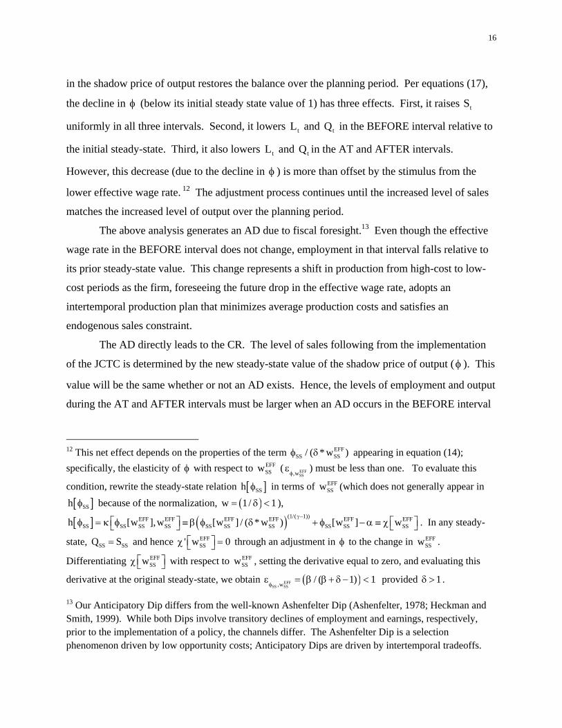
in the shadow price of output restores the balance over the planning period. Per equations (17),

the decline in (below its initial steady state value of 1) has three effects. First, it raises tS

uniformly in all three intervals. Second, it lowers tL and tQ in the BEFORE interval relative to

the initial steady-state. Third, it also lowers tL and tQ in the AT and AFTER intervals.

However, this decrease (due to the decline in ) is more than offset by the stimulus from the

lower effective wage rate. 12 The adjustment process continues until the increased level of sales

matches the increased level of output over the planning period.

The above analysis generates an AD due to fiscal foresight.13 Even though the effective

wage rate in the BEFORE interval does not change, employment in that interval falls relative to

its prior steady-state value. This change represents a shift in production from high-cost to low-

cost periods as the firm, foreseeing the future drop in the effective wage rate, adopts an

intertemporal production plan that minimizes average production costs and satisfies an

endogenous sales constraint.

The AD directly leads to the CR. The level of sales following from the implementation

of the JCTC is determined by the new steady-state value of the shadow price of output ( ). This

value will be the same whether or not an AD exists. Hence, the levels of employment and output

during the AT and AFTER intervals must be larger when an AD occurs in the BEFORE interval

12 This net effect depends on the properties of the term EFF

SS SS/ ( * w ) appearing in equation (14); specifically, the elasticity of with respect to EFF

SSw ( EFFSS,w

) must be less than one. To evaluate this

condition, rewrite the steady-state relation SSh in terms of EFFSSw (which does not generally appear in

SSh because of the normalization, w 1/ 1 ),

(1/( 1))EFF EFF EFF EFF EFF EFFSS SS SS SS SS SS SS SS SS SSh [w ],w [w ] / ( * w ) [w ] w

. In any steady-

state, SS SSQ S and hence EFFSS' w 0 through an adjustment in to the change in EFF

SSw .

Differentiating EFFSSw with respect to EFF

SSw , setting the derivative equal to zero, and evaluating this

derivative at the original steady-state, we obtain EFFSS SS,w

/ ( 1) 1 provided 1 .

13 Our Anticipatory Dip differs from the well-known Ashenfelter Dip (Ashenfelter, 1978; Heckman and Smith, 1999). While both Dips involve transitory declines of employment and earnings, respectively, prior to the implementation of a policy, the channels differ. The Ashenfelter Dip is a selection phenomenon driven by low opportunity costs; Anticipatory Dips are driven by intertemporal tradeoffs.

17

in order to compensate for the lost output. This extra output is the CR, the “compensating

rebound.”

Decreasing returns to labor, a downward-sloping demand curve, and an inventory

technology are each necessary for the AD and CR. If the returns to labor were increasing, then

the firm would have an incentive to bunch production in the AT interval absent inventory costs

in this restricted model.14 The absence of either of the remaining two conditions would lead to a

sequence of static optimization problems. If the firm faced a perfectly elastic demand curve,

then all of period t’s production could be sold without the penalty from declining marginal

revenues. In this case, the dynamic elements in the optimization problem disappear, the firm sets

period t production based only on the period t wage rate, and output and employment do not

change in the BEFORE interval.

Lastly, if there is no inventory technology, then tQ must equal tS in each period, and the

firm no longer has a separate sales decision.15 In this case, the inability to change inventory

prevents the firm from taking advantage of the differential production costs due to the delayed

implementation of the JCTC program. Again, the dynamic optimization problem becomes a

sequence of static problems, and there are no interrelations among wage rates in different periods.

With a concave production technology and a negatively-sloped demand curve, the firm has the

motivation to smooth sales and reallocate production but, absent an inventory technology, it does

not have the means to shift production across periods. All three elements are needed to provide

the firm the motivation and means to shift employment and generate ADs and CRs.

II.E. Responses To A JCTC: No Inventory Costs

We now relax one of the two restrictions in the above model and analyze the effects of

the rolling base on the response to the delayed JCTC. The qualitative effects on employment are

identical to those documented in sub-section II.D, though the quantitative effects differ. With a

14 If the returns to labor were constant, the firm would be indifferent to producing in any period other than the first. 15 If an inventory technology is not available to the firm, the inventory accumulation constraint t t t t 1I Q S I would be removed from the optimization problem (equation (8a)) and tS would be replaced by tQ for all t.

18

rolling base, the effective wage (equation (10b)) is impacted differently in the BEFORE interval

and then in the AT and AFTER intervals,

EFFt

t

w w * R w * 1/ 1 0 t BEFORE

, (18a)

EFFt

t

w w * 1 R w * / 1 0 t AT,AFTER

. (18b)

Somewhat paradoxically, the introduction of the JCTC raises the effective wage rate in the

BEFORE interval. With a delayed JCTC, the firm is not eligible to receive the tax credit in the

BEFORE interval, and hence obtains no benefits. However, any hiring in the BEFORE interval

raises the employment base above which subsequent employment must rise in order to qualify

for the credit. Hence, employment in the BEFORE interval lowers the value of the credit in

future periods. Being forward-looking, the firm internalizes this cost when choosing

employment in the BEFORE interval. This negative effect on profitability is measured in

equation (18a) by the discounted wage rate.

In the AT and AFTER intervals, the JCTC lowers effective wages. However, the

quantitative impact is dramatically reduced by the rolling base feature of the tax credit. The

/ 1 term in equation (18b) reflects that, with a rolling base, eligible incremental

employment receives a tax credit today but at the expense of eliminating the tax credit on

incremental employment tomorrow. This latter cost is discounted and, hence the overall

stimulus from the tax credit increases with the discount rate. Since the discount rate is generally

a small number, the rolling base feature drives a large wedge between the legislated and effective

tax credits and affects the specification of the JCTC in the econometric equation. Assuming an

expected long-run nominal return on equity of 10% and an expected long-run inflation rate of

3%, is 7%, and ( / (1 )) 0.065 . Hence, after the qualifying date, the effective tax credit

rate is only 6.5% of the legislated credit rate. In the extreme with no discounting ( 0 ), the

credit provides no stimulus at all.

II.F. Responses To A JCTC: The General Model

This sub-section analyzes the general model in which the JCTC is delayed and has a

rolling-base and, unique to this sub-section, inventory imbalances are costly. We introduce the

latter effect by allowing 0 . The first-order conditions for the general model are modified by

19

including terms containing the cost of inventory imbalances ( interacted with the

inventory/sales target, ) and the shadow price of adding to inventory imbalances ( t ),

( /( 1))

EFFtt t t 1EFF

t

L w w * 1 *R t BEFORE*w

, (19a)

( /( 1))

EFFtt t t t 1EFF

t

L w w * 1 *R t AT,AFTER*w

, (19b)

t 1 t SSt 2

* * IS t BEFORE,AT,AFTER*

. (19c)

The introduction of costly inventory changes the quantitative but not the qualitative

effects of the JCTC analyzed above. With tS and held at their initial steady-state levels,

employment initially decreases in the BEFORE interval and increases in the AT and AFTER

intervals. The BEFORE response in employment results in an inventory drawdown, t 0 (per

equation (9b)), and incremental employment in all periods becomes more valuable by reducing

the inventory imbalance. Consequently, an unambiguous implication of the general model is that

inventory costs lead to a smaller fall in employment in the BEFORE interval.

The relative change in employment in the AT and AFTER intervals is subject to two

contrasting effects and the net effect of the introduction of inventory costs is ambiguous. Since

the inventory drawdown in the BEFORE period is lower, there is a reduced need to replenish

inventory and relative employment falls. However, in the AT and AFTER intervals, there is an

added incentive to hire labor and produce output to eliminate the costly inventory imbalance, and

relative employment rises.

Inventory, its shadow price, and sales respond differently in subsequent periods relative

to the model in sub-section II.E. In the face of a negative inventory imbalance, an incremental

sale aggravates the imbalance and becomes less valuable in a model with costly inventory. The

inventory imbalance is largest in the BEFORE interval and falls over time. The decrease in the

imbalance results in an increase in t that stimulates sales. Rather than being constant over the

planning period, sales in the general model rises over time. As in all models considered here,

adjusts so that the inventory imbalance is eliminated by the end of the planning period at which

time T 0 .

20

Figure 5 summarizes the theoretical predictions for the path of employment over the

planning period and the interesting dynamics associated with a delayed JCTC. With a delayed-

JCTC, employment falls after the credit is enacted (at date St ) as forward-looking firms delay

hiring and draw down inventories to meet current demand. This decline is amplified when the

value of the tax credit is computed with a rolling base. The combined effect is illustrated by line

segment AB. When the JCTC goes into effect (at qualifying date Qt ), employment rises sharply

for several reasons: rebuilding the work force (line segment BC), responding to the lower

effective wage rate (line segment CD), and replenishing inventory (line segment DE). Note that

only the response indicated by line segment CD represents the “true” short-run stimulative effect

of a JCTC. Gradually, employment falls as inventories return toward their steady-state levels,

but it remains above the original employment level because of lower labor costs (line segment

AF, which is the same length as line segment CF).

In sum, the Anticipatory Dip is represented by line segment AB and Compensating

Rebound by line segments BC and DE.

II.G. Immediate-JCTC vs. Delayed-JCTC Regimes

The above analysis has focused on a firm facing a delayed-JCTC, which has been

adopted by seven states between 1990 and 2009. For a JCTC that goes into effect immediately,

as is the case in 14 states, the pattern of employment in the AT and AFTER intervals is

qualitatively similar to those displayed in Figure 5. An important difference is that fiscal

foresight and the associated ADs and CRs are not in force. For immediate-JCTC states, where

firms qualify for the JCTC at Qt , the employment increase in the AT interval will be smaller

than it is for firms in the delayed-JCTC states because there is no need to compensate for

deferred hiring and inventory drawdowns; that is, the CR does not exist. Thus, analyzing

employment responses in immediate-JCTC states provides a clean read on the true effectiveness

of JCTCs (line segment CD), whereas employment responses in delayed-JCTC states with

implementation lags are likely to overstate the effectiveness of tax credits (by the sum of the line

segments BC and DE). These predictions are summarized in Table 1 and lead to three

hypotheses about employment growth that we test:

21

1. Anticipatory Dips (ADs): the negative response in the BEFORE interval for delayed-

JCTC states;

2. Compensating Rebounds (CRs): the positive responses in the AT intervals for both

delayed-JCTC and immediate-JCTC states, with the former being larger than the latter;

3. Cumulative Effects (CUMs): the positive responses over the BEFORE, AT, and AFTER

intervals, taken as a whole, for both delayed-JCTC and immediate-JCTC states.

III. EMPIRICAL PRELIMINARIES AND SPECIFICATION ISSUES

III.A Employment and JCTC Data

Our empirical work focuses on the relation between JCTCs and employment. The latter

is measured by monthly, seasonally adjusted, private non-farm employment data for the period

January 1990 to December 2010.16 The earlier date is the first month in which these data are

published by the Bureau of Labor Statistics. The latter date is chosen because it provides at least

three years of employment data after the final JCTC in our sample.

The JCTCs are credits against a state's corporate income or franchise tax. We conducted

an initial state-by-state search for JCTCs from various sources to identify an exhaustive list of

permanent, broad-based JCTCs adopted and put into effect prior to December 2007, the official

NBER start date of the Great Recession. We restrict our focus to JCTCs that are “permanent,” in

the sense that their legislation did not set an expiration date, in order to rule out temporary

JCTCs that are sometimes passed as short-run stimulus measures (i.e., countercyclical fiscal

policies). These temporary JCTCs are likely to be endogenous with respect to current and

expected employment growth. Similarly, we exclude JCTCs passed during the Great Recession

or the weak subsequent recovery to avoid potential endogeneity concerns.17

16 The employment data come from the BLS’s Current Employment Statistics series. For details on the BLS, see http://www.bls.gov/bls/empsitquickguide.htm#payroll.

17 Wilson (2012) documents the large cross-state differences in the federal stimulus provided by the 2009 American Recovery and Reinvestment Act and finds that the stimulus spending had a substantial impact on state employment. See, also, Neumark and Grijalva (2013) for a study of the impact of JCTCs during the Great Recession.

22

For each credit, we hand-collected information on the signing date, the qualifying date,

the pecuniary value of the tax credit, and other relevant characteristics. For the period 1990 to

2007, we identified 21 JCTC adoptions. Details about the identification, valuation, and design of

JCTCs are provided in Appendix B.

Table 2 presents summary statistics for the employment level (in thousands), employment

growth rate (in percentage points), and pecuniary value of the JCTC sorted by the JCTC status of

states. As shown by the median values in panel A, column 2, the median delayed-JCTC state is

similar in size to the median non-JCTC state, while the median immediate-JCTC state is larger.

In panel B, the median growth rate for delayed-JCTC states of 0.138% is somewhat larger than

the comparable statistic of 0.110% for immediate-JCTC states. Both are somewhat below the

median growth rate for non-JCTC states of 0.155%. Panel C documents that JCTCs tend to be

more generous in the immediate-JCTC states. These latter two relations suggest that an

evaluation of possible bias arising from the endogeneity of JCTC adoption with respect to

employment growth is warranted.

Thus, before analyzing the impact of JCTCs on employment growth in Section IV, we

first study the JCTC adoption decision and determine the statistical properties of the employment

data. These results inform the specification of our empirical model in sub-section D.

III.B. Understanding JCTC Adoption

Apart from developing a better general understanding of JCTCs, analyzing the adoption

decision is useful for assessing and correcting for any endogeneity of JCTC adoption with

respect to recent employment growth. It is worth noting that, for several of the JCTCs in our

sample, the enacting legislation includes an explicit statement of objectives. In each case, the

legislation emphasizes longer-term economic development objectives and/or state

competitiveness and not short-term stimulus. Here are a few examples:

* The Arkansas General Assembly recognizes that job creation and capital investment in Arkansas is dependent upon being competitive with other states for business locations and expansions. * The objective of the job creation tax credit is to increase the number and quality of new jobs in [Maryland] by encouraging: A. Significant expansions of existing private sector enterprises; B. Establishment of new private sector enterprises; C. Creation of family supporting jobs; and D. Revitalization of neighborhoods and commercial areas.

23

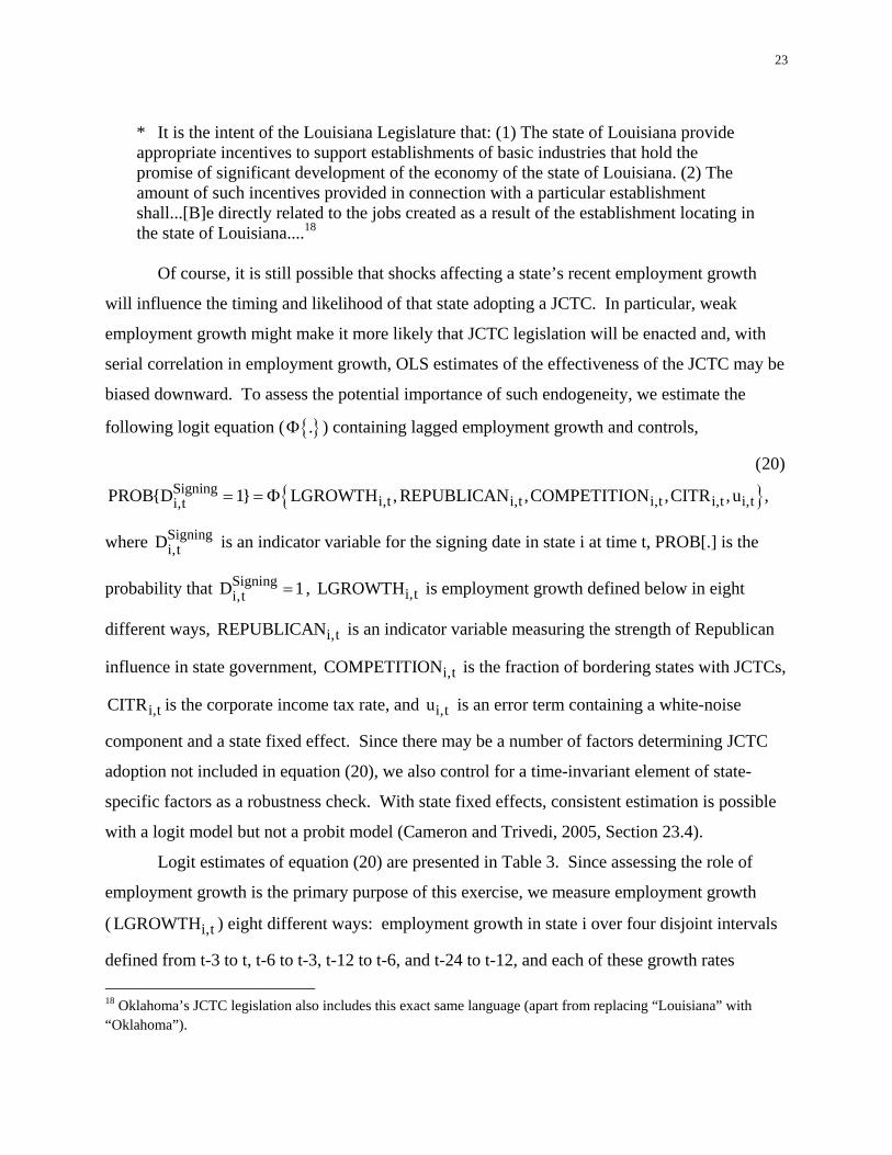
* It is the intent of the Louisiana Legislature that: (1) The state of Louisiana provide appropriate incentives to support establishments of basic industries that hold the promise of significant development of the economy of the state of Louisiana. (2) The amount of such incentives provided in connection with a particular establishment shall...[B]e directly related to the jobs created as a result of the establishment locating in the state of Louisiana....18

Of course, it is still possible that shocks affecting a state’s recent employment growth

will influence the timing and likelihood of that state adopting a JCTC. In particular, weak

employment growth might make it more likely that JCTC legislation will be enacted and, with

serial correlation in employment growth, OLS estimates of the effectiveness of the JCTC may be

biased downward. To assess the potential importance of such endogeneity, we estimate the

following logit equation ( . ) containing lagged employment growth and controls,

Signingi,t i,t i,t i,t i,ti,t

(20)

PROB{D 1} LGROWTH , REPUBLICAN ,COMPETITION ,CITR ,u ,

where Signingi,tD is an indicator variable for the signing date in state i at time t, PROB[.] is the

probability that Signingi,tD 1 , i,tLGROWTH is employment growth defined below in eight

different ways, i,tREPUBLICAN is an indicator variable measuring the strength of Republican

influence in state government, i,tCOMPETITION is the fraction of bordering states with JCTCs,

i,tCITR is the corporate income tax rate, and i,tu is an error term containing a white-noise

component and a state fixed effect. Since there may be a number of factors determining JCTC

adoption not included in equation (20), we also control for a time-invariant element of state-

specific factors as a robustness check. With state fixed effects, consistent estimation is possible

with a logit model but not a probit model (Cameron and Trivedi, 2005, Section 23.4).

Logit estimates of equation (20) are presented in Table 3. Since assessing the role of

employment growth is the primary purpose of this exercise, we measure employment growth

( i,tLGROWTH ) eight different ways: employment growth in state i over four disjoint intervals

defined from t-3 to t, t-6 to t-3, t-12 to t-6, and t-24 to t-12, and each of these growth rates 18 Oklahoma’s JCTC legislation also includes this exact same language (apart from replacing “Louisiana” with “Oklahoma”).

24

relative to the average employment growth rate in the states bordering state i. Either individually

or jointly, prior employment growth is not closely correlated with the JCTC adoption decision.

Tests of the joint significance of employment growth rates (bottom of Table 3) have p-values

that very far from conventional significance levels. There is a marked difference in the

coefficient estimates between column 1 (where state fixed effects are omitted) and the other four

columns (where they are included and states without a JCTC are dropped because their

dependent variable has no within-state variation). Importantly, there is no evidence indicating

that employment growth influences JCTC adoptions in our sample.

For models including state fixed effects (columns 2 to 5), JCTC adoptions are influenced

positively by competition from tax policies of bordering states and negatively by changes in

own-state corporate income tax rates. The latter result suggests that business tax policies are

considered as a package that encompasses both a reduction of business capital taxes and the

adoption of JCTCs (Wildasin, 2007). Both coefficients are statistically significant regardless of

the definition of employment growth. By contrast, there is no discernible relation between

political party and JCTC adoption.

In sum, the results in Table 3 suggest that JCTCs are adopted as longer-term tax policy

measures in response to a general desire to cut business taxes, promote economic development,

and improve the state’s competitiveness. They do not appear to be short-term, countercyclical

policies responding to anemic employment. Most importantly for the validity of our estimates,

there is no evidence for reverse causation from lagged employment growth to JCTC adoption.

Nonetheless, as an additional safeguard against the adverse impact of endogeneity, we utilize

these logit estimates for inverse probably weighting in our main empirical models, as explained

in Section III.D.

III.C. Properties of the Monthly Employment Data

The statistical properties of the monthly employment data are important for proper

specification of the econometric equation relating employment to JCTCs. We access stationarity

with informal and formal tests. We first estimate models with log employment and the first-

difference of log employment as the dependent variable and the same set of independent

variables: current, lagged (12 months), and led (12 months) dummies for the effective date of

the JCTC and various lags of the dependent variable (LDV).

25

For the log levels equation, the LDV coefficient (when only one LDV is included) is

close to one. For additional lags of the LDV, the sum of LDV coefficients is greater than one.

Thus, the log levels equation would not appear to be a suitable specification for employment.

By contrast, for the log difference equation, the LDV coefficient (when only one LDV is

included) is close to zero. Additional lags of the LDV yield coefficient sums that become

positive and statistically significant, but the near constancy of the R2 s suggests that there is little

additional explanatory power provided by extra lags. These results strongly suggest that

employment is best modeled as a simple growth rate.

This initial conclusion is confirmed by a formal unit root test (Pesaran, 2007) that extends

the standard augmented Dickey-Fuller test to allow for cross-sectional dependence. This test

indicates that the log employment series has a unit root and confirms that employment is best

modeled as a simple growth rate.

Taken together, the results presented in Section III.B and IIII.C indicate that an

estimating equation with employment growth as the dependent variable and a measure of JCTCs

as an independent variable will deliver consistent parameter estimates.

III.D. Specification Of The Estimating Equation

With these conclusions in mind, we derive a regression specification relating employment

growth to JCTCs and other likely determinants of employment growth,

Del Deli, t j i, t jBEFORE AT Del AFTER

Del Del i, t DelBEFORE AFTERi

Immi, t jAT Del AFTER

Imm i, t Imm AFTER

BEFORE AFTERi

After

i,t i,t 1j 1 j 1

j 1

i,t i,t

J J

J

D DL / L D

J J

DD

J

X u .

(21)

Deli, tD is an indicator variable that equals one in the qualifying month for a delayed-JCTC state

and equals zero otherwise. Immi, tD is an indicator variable that equals one in the latter of the

signing month and qualifying month for an immediate-JCTC state and equals zero otherwise. BEFOREiJ is the length of the BEFORE interval for state i determined by the nature of each state’s

JCTC legislative history and the resulting “distance” between the signing and qualifying dates;

the i subscript indicates that the distance will vary by state. The AT interval is only one month

26

long. AFTERJ is the length of the AFTER interval, which is assumed to be the same for all states.

We will present models with AFTER interval lengths of 12, 24, and 36 months.19 The purpose

of dividing by the interval lengths is so that the 's will reflect average monthly growth rate

effects and can be compared across intervals of different lengths. i,tX represents control

variables, i,tu is an error term that contains three components (discussed below) and

and the 's are parameters to be estimated.

As highlighted by the theoretical model, there exists multiple intervals (BEFORE, AT,

AFTER) in which employment is expected to respond differently to the JCTC. The object of our

analysis is to generate consistent estimates of the 's for each interval and across the delayed-

JCTC and immediate-JCTC regimes. Equation (21) is not a first-order condition from a

structural model, and the 's should not be interpreted as a structural parameter.20 Rather, the

's are average treatment effects measuring the impact of the JCTC, by regime, on a monthly

basis over an interval. Specifically, BEFOREDel is the average effect of a JCTC in a delayed-JCTC

state on monthly employment growth during the BEFORE interval; ATDel ( AT

Imm ) is the average

effect of a JCTC in a delayed-JCTC (immediate-JCTC) state during the AT interval; and AFTERDel

( AFTERImm ) is the average effect of a JCTC in a delayed-JCTC (immediate-JCTC) state during the

AFTER interval.

The vector Xi,t in equation (21) represents four control variables included in the baseline

model. One way to control for overall demand conditions in the state and avoid endogeneity

problems is to include a measure of the state’s exposure to particularly fast-growing or slow-

growing industries. For example, even in absence of any employment-inducing fiscal policies, a

state with a large IT industry during the late 1990s was likely to experience rapid employment

19 In the one case (Virginia) where the state repealed the JCTC, the AFTER interval is truncated if the number of months between the initial qualifying date and the withdraw date is less than the specified length of the AFTER interval (i.e., 12, 24. or 36 months).

20 Recall from equations (17) and the surrounding text that the response of employment to the JCTC depends directly on the JCTC and indirectly on the JCTC-induced movement in .

27

growth during that period. We control for industry-driven employment changes by first

predicting a state’s year-over-year employment growth rate with a weighted-average across

industries of the national (excluding own-state) employment growth rates (year-over-year),

where the weights are the state’s employment shares in each industry. Multiplying this predicted

annual growth rate by the level of own-state employment in period t - 12 yields a predicted level

of employment in period t. This “predicted” employment variable, Pi,tL , was introduced by

Bartik (1991) and is frequently referred to as the “Bartik shift-share variable.” If the state is

small relative to the nation, then this variable will not be correlated with the error term. Our

empirical model is stated in terms of monthly growth rates, we therefore add the monthly growth

rate of this predicted employment variable, P Pi,t i,t 1L / L , to our baseline specification.

The three other control variables were included previously in the logit model. Section

III.B documented that the adoption of a JCTC is positively influenced by JCTCs in effect in

bordering states. Since one of the underlying channels of influence may be the effect of

bordering state JCTCs on state i’s employment, we include i,tCOMPETITION as an additional

control variable. The i,tCITR was also statistically significant in the logit model. Lastly, we

include i,tREPUBLICAN as a fourth control variable for completeness.

We model the error term in equation (21) with a conventional two-way error components

structure,

i,t i t i,tu , (22)

where i is a state-specific effect (for the employment growth rate), t is a time fixed effect,

and i,t is a white noise error term.

Substituting equations (22) into equation (21) and inserting the four control

variables, we obtain the following estimating equation,

28

Del Deli, t j i , t jBEFORE AT Del AFTER

Del Del i, t DelBEFORE AFTERi

Immi, t jAT Del AFTER

Imm i, t Imm AFTER

BEFORE AFTERi

After

j 1 j 1

P Pi,t i,t 1

j 1

J Ji,t i,t 1

J

1

2 i,t 3 i

D DL / L D

J J

DD + L / L

J

COMPETITION TAXRATE

,t 4 i,t

i t i,t

REPUBLICAN

(23)

where the non-JCTC states serve as the control group.

We make one minor adjustment to the JCTC indicator variables above so that the

estimated 's can be interpreted as the effects of JCTCs on eligible firms. Only firms that are

not contracting are eligible to use JCTCs, so we multiply the indicator variables by the fraction

of firms in this situation ( i,tELIGIBLE ). The latter variable equals one minus the fraction of

establishments in the state that are contracting according to the Business Employment Dynamics

data from the Bureau of Labor Statistics. Our results are robust to excluding this adjustment, as

shown in in Section IV.C.

Equation (23) uses simple indicator variables to represent the effects of the JCTCs and is

our baseline model. However, an indicator variable cannot account for variation across states

and intervals in the value of the tax credit. As indicated by the theoretical model, there are subtle

relations between the JCTC and its ultimate incentive effects that may vary by state and by

interval within a state. As an extension to the baseline empirical model, we also estimate a

specification which attempts to capture this variation in pecuniary incentives. Specifically, we

compute the logarithmic time differences of the effective wage rates entering the first-order

conditions in equations (19) for the BEFORE and AT intervals.21 We further assume that

variations in JCTCs have no effect on the gross-of-JCTC wage rate and that the non-JCTC

induced changes in the wage rate are captured by time and state fixed effects (discussed below).

21 This stimulus term is zero for the AFTER interval. That is, the JCTC adopted in the AT interval provides no additional stimulus in the AFTER interval. Nonetheless, we allow for lagged effects of the AT interval’s stimulus by including JAFTER lags of it in the baseline estimating equation, similar to the

inclusion of JAFTER lags of Deli , t jD and Im m

i, t jD in the indicator variable specification (equation 23).

29

III.E. Inverse Probability Weighting (IPW)

While our logit estimates suggest that selectivity with respect to employment growth is

not a problem that will adversely affect our estimates, endogeneity may occur for other reasons,

especially arising from omitted variables. In order to further guard against the possible distorting

effects, we obtain coefficient estimates using an Inverse Probability Weighting (IPW) estimator.

The IPW is a type of matching estimator and is implemented in a two-step procedure (Hirano,

Imbens, and Ridder, 2003). First, we use the logit model to estimate probabilities of “treatment”

(i.e., the adoption of a JCTC) and non-treatment. We then estimate our main empirical model

(equation 23) using weighted least squares. The weight for each treated observation is the

estimated inverse probability of treatment for that observation (given its values for the variables

that go into the logit model). The weight for each non-treated observation is the estimated

inverse probability of non-treatment (i.e., the inverse of one minus the probability of treatment)

for that observation. Thus, the IPW is putting more weight on treated observations that are

unlikely to have been treated and more weight on untreated observations likely to have been

treated. This weighting moves the adjusted data closer to a randomized experiment (where all

observations are equally likely to be treated).

The IPW works well when there is a close correspondence between the domains of the

densities of the probability of a JCTC signing for those states that have adopted and those that

have not adopted. The kernel densities of the probability of a JCTC signing presented in Figure

6 suggest that this criterion has been met with the current application of the IPW. Moreover, as

we shall see below, IPW and OLS (i.e., equal-weighted IPW) estimates are quite similar, sug-

gesting informally that selectivity and omitted variables biases are a minimal concern in our data.

IV. EMPIRICAL RESULTS

This section presents estimates of the impact of JCTCs on employment growth that allow

us to assess the three key empirical relations summarized in Table 1:

1. The AD (Anticipatory Dip): BeforeDel 0 ,

2. The CR (Compensating Rebound): At AtDel Imm ,

3. The CUM (Cumulative Effects): ImmDelCUM 0; CUM 0 .

30

Our baseline estimates are with the JCTC measured by an indicator variable and are presented in

sub-section A. The robustness of these results is examined in the additional empirical results

presented in sub-sections B and C.

IV.A. Baseline Estimates

Table 4 contains our baseline estimates of the coefficients for the three intervals for the

delayed regime and the two intervals for the immediate regime , as well as their cumulative sums.

The s for the five intervals represent the conditional average employment growth per month (in

percentage points) and are based on equation (23). The Cumulative Effect sums the product of

each and the number of months in its interval for either the delayed or immediate regime. The

length of the BEFORE interval varies by state, so we use its average length, 5.25 months, for this

calculation. The length of the AFTER interval varies across the three sets of results for 12, 24,

and 36 months. The standard errors are robust to heteroskedasticity and to clustering of residuals

by state. State clustering allows for general serial correlation of residuals as recommended in

Bertrand, Duflo and Mullainathan (2004).

We begin with the results in the first two columns for an AFTER interval of 12 months.

For the delayed regime, the coefficient in the BEFORE interval is -0.068 and statistically

significantly different from zero. This coefficient means that employment growth in delayed-

JCTC states during the credit implementation period is 0.068 percentage points lower than it

would have been without the credit adoption. This represents about a 50% reduction relative to

the median monthly employment growth in delayed-JCTC states of 0.138 (see Table 2). Since

the implementation period averages 5.25 months, this reduction in growth implies an average

reduction in the level of employment over the BEFORE interval of -0.357 (-0.068*5.25)

percentage points. An AD is clearly identified for the delayed regime.

In the AT interval, the coefficients for the delayed and immediate regimes are 0.141 and

0.036, respectively. The coefficient for delayed states implies roughly a doubling of employment

growth in the AT month relative to median employment growth for these states. The difference

in the AT coefficients between the delayed and immediate states measures the CR. For the

regression in columns 1 and 2, when the AFTER interval is 12 months, this difference of 0.105,

which is economically large but not quite statistically significant (with a p-value of 0.12).

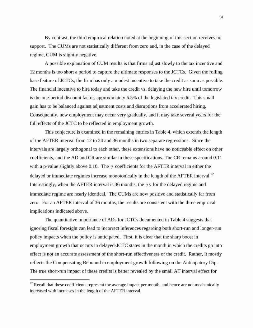
31

By contrast, the third empirical relation noted at the beginning of this section receives no

support. The CUMs are not statistically different from zero and, in the case of the delayed

regime, CUM is slightly negative.

A possible explanation of CUM results is that firms adjust slowly to the tax incentive and

12 months is too short a period to capture the ultimate responses to the JCTCs. Given the rolling

base feature of JCTCs, the firm has only a modest incentive to take the credit as soon as possible.

The financial incentive to hire today and take the credit vs. delaying the new hire until tomorrow

is the one-period discount factor, approximately 6.5% of the legislated tax credit. This small

gain has to be balanced against adjustment costs and disruptions from accelerated hiring.

Consequently, new employment may occur very gradually, and it may take several years for the

full effects of the JCTC to be reflected in employment growth.

This conjecture is examined in the remaining entries in Table 4, which extends the length

of the AFTER interval from 12 to 24 and 36 months in two separate regressions. Since the

intervals are largely orthogonal to each other, these extensions have no noticeable effect on other

coefficients, and the AD and CR are similar in these specifications. The CR remains around 0.11

with a p-value slightly above 0.10. The coefficients for the AFTER interval in either the

delayed or immediate regimes increase monotonically in the length of the AFTER interval.22

Interestingly, when the AFTER interval is 36 months, the s for the delayed regime and

immediate regime are nearly identical. The CUMs are now positive and statistically far from

zero. For an AFTER interval of 36 months, the results are consistent with the three empirical

implications indicated above.

The quantitative importance of ADs for JCTCs documented in Table 4 suggests that

ignoring fiscal foresight can lead to incorrect inferences regarding both short-run and longer-run

policy impacts when the policy is anticipated. First, it is clear that the sharp boost in

employment growth that occurs in delayed-JCTC states in the month in which the credits go into

effect is not an accurate assessment of the short-run effectiveness of the credit. Rather, it mostly

reflects the Compensating Rebound in employment growth following on the Anticipatory Dip.

The true short-run impact of these credits is better revealed by the small AT interval effect for 22 Recall that these coefficients represent the average impact per month, and hence are not mechanically increased with increases in the length of the AFTER interval.

32

immediate-JCTC states. Another way to see this point is to consider what inference researchers

might draw if they evaluated the impact of JCTCs using the standard event study approach,

ignoring fiscal foresight. In that case, they would not distinguish between delayed- and

immediate-JCTC states and they would not account for any potential drop in employment growth

prior to the AT interval. In other words, they would simply regress employment growth on the

JCTC indicator in the AT interval (along with controls and state and month fixed effects). We

find that such a regression yields an AT effect of 0.072 (with a p-value of 0.036), roughly double

the size of the AT interval effect for immediate-JCTC states from Table 4. Again, this estimate

would give a misleading impression of the effectiveness of JCTCs because part of this effect is

due to fiscal foresight, specifically the CR for the delayed-JCTC states.

Second, ignoring fiscal foresight can also lead to incorrect inferences regarding the

longer-run impact of JCTCs. Consider the estimated cumulative effect of JCTCs on employment

in Table 4 when AFTER equals 36 months. We see that the cumulative effect for delayed-JCTC

states would be raised by 33% (to 1.318 from 0.992) if we ignored the decrease during the

BEFORE interval.23

IV.B. An Alternative Measure Of The JCTC

Measuring the JCTC with an indicator variable has the advantage that it is likely to have

much less measurement error than a variable that reflects the complexities of the legislated tax

code (e.g., refundability, transferability, tax credit caps) that cannot be reflected in a single figure.

In such a situation, using a coarse categorical variable may lead to less biased econometric

estimates. Nonetheless, the baseline results could be misleading if the effective JCTC is

relatively higher for delayed-JCTC states. In this case, the larger increase we observe at the AT

intervals may be due to the larger effective JCTCs, not the CR effect that seems to be

documented in Table 4. The summary statistics suggest that this is not a concern, as the median

credit value, as a percent of the state’s average manufacturing wage, for delayed-JCTC states is

3.2%, while that for immediate-JCTC states is 5.0% (see Table 2, Panel C). Also, our theoretical

model indicates that the employment growth incentives induced by JCTCs vary by regime and

interval and hence one might expect different effects of JCTCs across regimes and intervals.

23 This figure is computed as follows: 1.318 = (0.992-AD), where AD = -0.326 (= -0.062 * 5.25 months), where 5.25 months is the average length of the BEFORE interval.

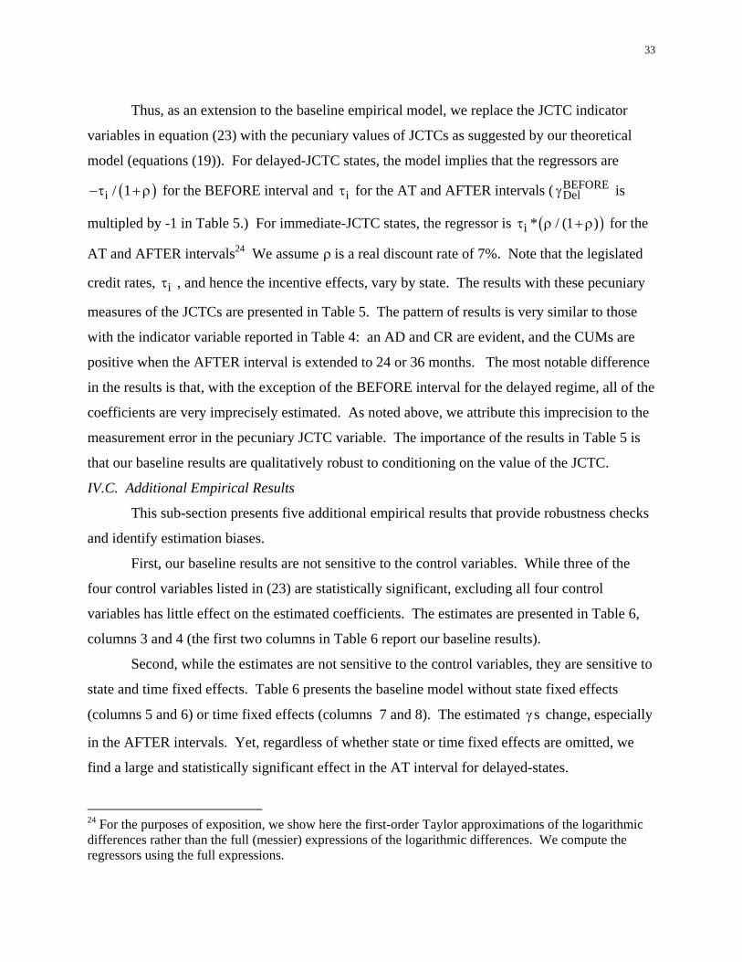
33

Thus, as an extension to the baseline empirical model, we replace the JCTC indicator

variables in equation (23) with the pecuniary values of JCTCs as suggested by our theoretical

model (equations (19)). For delayed-JCTC states, the model implies that the regressors are

i / 1 for the BEFORE interval and i for the AT and AFTER intervals ( BEFOREDel is

multipled by -1 in Table 5.) For immediate-JCTC states, the regressor is i * / (1 ) for the

AT and AFTER intervals24 We assume is a real discount rate of 7%. Note that the legislated

credit rates, i , and hence the incentive effects, vary by state. The results with these pecuniary

measures of the JCTCs are presented in Table 5. The pattern of results is very similar to those

with the indicator variable reported in Table 4: an AD and CR are evident, and the CUMs are

positive when the AFTER interval is extended to 24 or 36 months. The most notable difference

in the results is that, with the exception of the BEFORE interval for the delayed regime, all of the

coefficients are very imprecisely estimated. As noted above, we attribute this imprecision to the

measurement error in the pecuniary JCTC variable. The importance of the results in Table 5 is

that our baseline results are qualitatively robust to conditioning on the value of the JCTC.

IV.C. Additional Empirical Results

This sub-section presents five additional empirical results that provide robustness checks

and identify estimation biases.

First, our baseline results are not sensitive to the control variables. While three of the

four control variables listed in (23) are statistically significant, excluding all four control

variables has little effect on the estimated coefficients. The estimates are presented in Table 6,

columns 3 and 4 (the first two columns in Table 6 report our baseline results).

Second, while the estimates are not sensitive to the control variables, they are sensitive to

state and time fixed effects. Table 6 presents the baseline model without state fixed effects

(columns 5 and 6) or time fixed effects (columns 7 and 8). The estimated s change, especially

in the AFTER intervals. Yet, regardless of whether state or time fixed effects are omitted, we

find a large and statistically significant effect in the AT interval for delayed-states.

24 For the purposes of exposition, we show here the first-order Taylor approximations of the logarithmic differences rather than the full (messier) expressions of the logarithmic differences. We compute the regressors using the full expressions.

34

Third, we check whether our baseline results are sensitive to the adjustment we made to

the JCTC variable for the fraction of firms that are not contracting and therefore eligible to

receive a tax credit. When we repeat the baseline regression without the eligibility adjustment

for the JCTC variable, there is little effect on the estimates. This result likely owes to the fact

that the fraction of ineligible firms is small (about 7% over the sample of JCTC states) and varies

little across states.

Fourth, a perennial concern in policy event studies is selectivity. In the present case, it is

possible that deficient employment growth might lead to the passage of JCTC legislation. This

concern has been addressed and largely discounted by the logit models presented in Section III.B

and Table 3. Moreover, the Inverse Probability Weighting (IPW) estimator discussed in Section

III.E adjusts for selectivity or, more generally, various sources of endogeneity that may bias

estimates. An informal test for the importance of endogeneity is to compare the IPW and OLS

estimates, the latter possibly influenced by endogeneity. The OLS estimates prove to be very

similar to those presented previously in Table 4. For an AFTER interval of 36 months, we have

BEFORE = -0.063 [p = 0.011], ATDel = 0.127 [0.016], ATImm = 0.054 [0.158], AFTERDel =

0.028 [0.024], AFTERImm = 0.028 [0.012], CUMDel = 0.817 [0.063], CUMImm = 1.058 [0.011].

Fifth, the tax competition literature suggests that JCTC-induced increases in employment

growth might create interstate spillovers, which could be negative or positive. In particular, a

JCTC in one state could draw jobs away from other states or, alternatively, the stimulus to

economic activity in the JCTC state could “leak” out to other states via induced upstream

demand. Understanding spillovers is of particular importance if our results based on state tax

credits are to inform the policy debates surrounding a potential federal JCTC. If negative

(positive) spillovers exist, then our estimates are an upper (lower) bound on the likely effect of a

federal tax credit because interstate mobility of labor and intermediate inputs is much greater

than international mobility.

To examine spillovers, we analyze the effect of JCTCs on employment growth in

neighboring states. If the employment growth associated with a JCTC is largely coming at the

expense of neighboring states, then we would expect the JCTC for state i to have a negative

impact on employment growth in neighboring states. Conversely, if there is leakage of induced

upstream demand to neighboring states, we would expect a given state’s JCTC to have a positive

impact on employment growth in those states. We test these propositions by forming for state i

35

its spatial lag of employment growth. The spatial lag is simply an equal-weighted average of

employment growth in neighboring-qua-bordering states. We then run the following model,

which has the same specification as our baseline model (equation (23)) except that the dependent

variable is the spatial lag of employment growth instead of own-state employment growth,

BEFOREi Del Del

i,t j i,t jBEFORE At Del AfterDel Del i,t DelBEFORE AFTER

i

Immi,t jAt Imm AFTER

Imm i,t Imm AFTER

After

AFTER

JJ

i,t i,t 1j 1 j 1

JP P

1 i,t i,t 1j 1

2 i,t 3 i,t

D DS L / L D

J J

DD L / L

J

COMPETITION TAXRATE

4 i,t

i t i,t

REPUBLICAN

(24)

where S . is a spatial lag operator that weights only the bordering states and i,t is an error

term with a conventional two-way error components structure. The s are estimated

coefficients that capture interstate effects. The results are shown in Table 7. We find no

evidence of negative spillovers. Rather, the point estimates in Table 7 generally exhibit the same

signs as their corresponding estimates in Table 4, but with smaller magnitudes. For instance, we

find that in the month in which a delayed JCTC goes into effect, it has an impact (AT effect) on

neighboring states’ employment growth of nearly half the size of the effect in the JCTC state

itself (from Table 4). . The cumulative increase in employment in neighboring states due to the

enactment of a JCTC in a given state also is about half of the cumulative increase in employment

in the state itself, though it is not statistically significant. All in all, the results in Table 7 are

suggestive of modest positive spillovers from JCTCs to neighboring states.

IV.D. Cost Per Job Created

Are JCTCs effective state policy tools? How does the job creation they induce compare

to that achieved by other government policies? As a final exercise, we address these questions

by presenting a back-of-the-envelope calculation of the cost per job created (or retained) for the

average JCTC-adopting state.

The cost of a given state’s JCTC program over the event window from signing date ( Sit )

to 36 months after the qualifying date is:

Si

CFi i i i ii,t

C (g CUM )* L * w * , (25)

36

where Sit

L is the level of employment in state i as of its JCTC signing date, wi is its average

annual wage, i is the legislated credit rate (as a percentage of the wage), CUMi is the

cumulative growth rate of employment over the event window due to the credit, and CFig is the

(counterfactual) growth rate of employment that would have occurred in the absence of the

credit. Thus, Si

CFi i,t

g * L is the inframarginal amount of net job creation that gets subsidized via

the credit even though it would have occurred anyway, and Si

CFi i ii,t

g * L * w * is the total amount

of inframarginal subsidy.

The number of jobs created in a given state by its JCTC is given by:

Si

i i i,tJC CUM * L . (26)

Therefore, the cost-per-job (CPJi) created in state i is:

Si

Si

CF CFi i i ii,t i i i

i i ii ii,t Marginal

SubsidyInframarginalSubsidy

(g CUM ) * L * w * g * w *CPJ w *CUM * L CUM

. (27)

The first term of the final equation is the inframarginal subsidy, the cost of the credit that went to

subsidizing job creation that would have occurred anyway. The second term is the marginal

subsidy, the cost that went to subsidizing the job creation that was due to the credit.

We calculate the CPJ, along with the inframarginal and marginal components, for the

average delayed-JCTC state and for the average immediate-JCTC state. For the average

delayed-JCTC state, we calculate CFg by converting the average monthly employment growth

rate over delayed-JCTC states, excluding months in the event window, to a growth rate over 42

months, the average length of the event window for delayed-JCTC states. Similarly, for the

average immediate-JCTC state, we calculate CFg by converting the average monthly employment

growth rate over those states, excluding months in the event window, to a 37-month growth rate,

the length of the event window for immediate-JCTC states. We calculate the average nominal

credit value ( w * ), by regime, from the data described earlier on legislated credit rates and

average annual wages in manufacturing ($49,527 for delayed-states and $35,983 for immediate-

states). The average CUM, by regime, comes from Table 4 (with AFTER = 36 months) and is

approximately 0.01 for both regimes.

37

The results of these calculations are shown in Table 8. For the average delayed-JCTC

state, the cost per job created is $13,213. The marginal subsidy portion of that is simply the

average nominal credit per job, $2,159. The remaining $11,054, or 84%, is a subsidy to

inframarginal job creation. For the average immediate-JCTC state, the cost per job is $16,644,

of which 24% is due to the marginal subsidy and 76% is a subsidy to inframarginal job creation.

The average cost per job across all states is a little over $16,000, with nearly 80% of that being

an inframarginal subsidy.

Several other studies have quantified the effects of employment-related tax credits.25

Kesselman, Williamson, and Berndt (1977) estimate a translog cost function on U.S.

manufacturing data. Their estimates imply a cost per job created of $14,808, about 8% lower

than the figure based on our estimates in Table 8.26 Faulk (2002) examines an incremental job

tax credit in Georgia. With cross-section data, she estimates separate employment equations for

eligible firms that are participating or non-participating in the Georgia program and a probit

selection equation to determine participation. For those eligible firms participating in the

program, employment rose by between 23 to 28 percent. The cost was between $2,280 and

$2,680 per job created.

More recently, Bartik and Bishop (2009) undertake a detailed simulation exercise of a

temporary federal JCTC valued at 15% of the wage cost of new employment in 2010 and 10% in

2011. They conclude that the cost per job would be $4,656 in 2010 and $6,301 in 2011. These

estimates include important macroeconomic feedback effects. With these excluded, their

estimates can be compared to those in Table 8, and their estimated cost per job created is

approximately $37,000. Cahuc, Carcillo, and Le Barbanchon (2016) evaluate a French hiring

25 See Neumark (2013) and Neumark and Troske (2012) for surveys of this literature’s policy recommendations.

26 We compare the effective wage elasticities from the two studies. The Kesselmen, Williamson, and Berndt elasticity is based on the data in their Table 2, panel 4: column 1 (or column 2) for the wage change and column 7 for the employment change. (The resulting 0.13% elasticity is an average of the four entries in this table.) The Chirinko and Wilson elasticity is the average mean JCTC from Table 2, panel C, column 1, divided by the mean annual wages (see Section IV.D) for each regime. An average figure is based on weights of 1/3 and 2/3 for the delayed and immediate regimes, respectively. The Kesselmen et al. figure is 11% larger than the CUM figure of 1.0 that we used in Table 8. We insert CUMKesselmen into our algorithm for computing the cost per job created (equation (27)).

38

credit that was temporary, unexpected, and targeted to low income workers in very small firms.

Based on their estimated structural model, they conclude that the gross cost per job created for

this credit is about one fourth of the average annual wage, which would correspond to roughly

$10,000 in the U.S. They estimate a permanent credit in an environment of flexible wages

would have a cost per job 14 times larger.

The studies above focused specifically on job creation tax credits. Recent years have also

seen broader fiscal policy efforts aimed at stimulating employment growth. In particular, the

American Recovery and Reinvestment Act (ARRA) sought to stimulate employment growth

through a combination of federal spending and tax cuts. A number of recent studies have

estimated the cost per job of the ARRA spending. Wilson (2012) examined the impact of ARRA

spending on job creation at the state level using exogenous formula apportionment of ARRA

funds as an instrument for total ARRA spending by state. He estimated the cost of a job created

(or saved) from the spending to be around $125,000. This estimate falls roughly in the middle of

other cross-state analyses of the cost per job of ARRA spending, such as the $202,000 obtained

by Conley and Dupor (2013) and the $26,000 obtained by Chodorow-Reich, Feiveson, Liscow,

and Woolston (2012).

Thus, even the lowest estimates of the cost per job created from the broad fiscal stimulus

of the ARRA are well above our estimate of the cost per job associated with JCTCs. Moreover,

the JCTCs to which our cost per job created estimates apply are permanent JCTCs. The

evidence cited above indicates that the cost per job from temporary JCTCs is likely to be even

lower. This suggests temporary incentives targeted specifically at job creation may be more

cost-effective policies for stimulating employment than general government spending.

V. CONCLUSIONS This paper uses the experience of 21 U.S. states to inform policy discussions about fiscal

foresight and the effectiveness of job creation tax credits (JCTCs). The relevant legislative dates

for all broad-based state JCTCs passed in the U.S. since 1990 are compiled. Important for our

analysis of fiscal foresight, the JCTCs are of two types, ones that take effect with a delay and

others that take effect immediately. We develop a theoretical model that captures the effects of

the rolling base feature of JCTCs and shows that this feature is quantitatively very important.

39

The theoretical model highlights three key conditions necessary for the existence of fiscal

foresight and delivers a set of empirical predictions evaluated in an event study framework.

Our econometric estimates lead to several conclusions. Fiscal foresight matters. Based

on our unique dataset, we document the quantitative importance of Anticipatory Dips (ADs) and

Compensating Rebounds (CRs). This intertemporal behavior runs counter to policy objectives

and makes it difficult to accurately evaluate the impacts of fiscal policy. The evidence based on

JCTCs suggests that failing to account for the distorting effects of fiscal foresight can lead to a

substantial overstatement of the impacts of fiscal policy. For instance, we find that ignoring

fiscal foresight would overstate the estimated stimulus to employment growth by 33%.

We also find that the cumulative effect (CUM) of JCTCs is positive, but the effect takes

two to three years to be fully observed in the data. These long lags, coupled with evidence from

our logit analysis, suggest that the permanent state JCTCs we study in this paper are not

countercyclical tools adopted to address transitory weaknesses in employment. Rather, they

appear to be economic development policies with a longer run focus. Our estimates imply a cost

per job created by permanent state JCTCs of approximately $16,000. Given other studies in the

literature, these JCTCs appear to be quite cost effective compared with less targeted fiscal

initiatives aimed at stimulating employment such as the 2009 federal stimulus package, though

less cost effective than explicitly temporary JCTCs.

Our data collection effort revealed the surprising fact that many broad-based state JCTCs

have an implementation lag. The quantitatively important AD found in this study raises a

question: why would policymakers adopt legislation that would temporarily lower employment?

The CR documented in our empirical work indicates that there will be a big jump in employment

in the qualifying month and thus suggests an answer, albeit a cynical one. With a delayed JCTC,

politicians can point to the large boost to employment growth, which tends to occur in the first

month the credit goes into effect, as evidence of the wisdom of their policies and their concern

for the unemployed.

REFERENCES

Abadie, Alberto, Diamond, Alexis, and Hainmueller, Jens. “Synthetic Control Methods for Comparative Case Studies: Estimating the Effect of California’s Tobacco Control Program.” Journal of the American Statistical Association, 105 (2010), 493–505.

40

Ashenfelter, Orley. "Estimating the Effect of Training Programs on Earnings." Review of Economics and Statistics, 60 (1978), 47-57.

Auerbach, Alan J. and Gale, William. “Activist Fiscal Policy to Stabilize Economic Activity.” in Financial Stability and Macroeconomic Policy, Federal Reserve Bank of Kansas City. (2009), 327-374. Bartik, Timothy J. Who Benefits from State and Local Economic Development Policies? 1991.

Kalamazoo, Michigan, W.E. Upjohn Institute for Employment Research. Bartik, Timothy J. Jobs for the Poor: Can Labor Demand Policies Help? 2001. New York,

Russell Sage Foundation. Bartik, Timothy J., and John H. Bishop. "The Job Creation Tax Credit." Oct. 20, 2009. EPI

Briefing Paper #248. Bertrand, Marianne, Esther Duflo, and Sendhil Mullainathan. 2004. “How Much Should We

Trust Differences-in-Differences Estimates?” Quarterly Journal of Economics, 119(1): 249-275.

Blanchard, Olivier, and Perotti, Roberto. “An Empirical Characterization of the Dynamic Effects of Changes in Government Spending and Taxes on Output.” Quarterly Journal of Economics, 117 (2002), 1329-1368. Cahuc, Pierre, Carcillo, Stephane, Le Barbanchon, Thomas. “The Effectiveness of Hiring

Credits” Unpublished Manuscript, January 2016. Cameron, A. Colin, and Trivedi, Pravin K., Microeconometrics: Methods and Applications

(Cambridge: Cambridge University Press, 2005). Chodorow-Reich, Gabriel, Laura Feiveson, Zachary Liscow, and William Gui Woolston (2012).

“Does State Fiscal Relief During Recessions Increase Employment? Evidence from the American Recovery and Reinvestment Act,” American Economic Journal: Economic Policy 4(3): pp. 118-145.

Coglianese, John, Davis, Lucas W., Kilian, Lutz, and Stock, James H. “Anticipation, Tax

Avoidance, and the Price Elasticity of Gasoline Demand.” NBER Working Paper No. 20980. (February 2015).

Conley, Timothy G., and Bill Dupor. “The American Recovery and Reinvestment Act: Solely a

Government Jobs Program?” Journal of Monetary Economics, 60 (Jan. 2013), 535-549. Faulk, Dagney. “Do State Economic Development Incentives Create Jobs? An Analysis of State

Employment Tax Credits.” National Tax Journal, 55 (June 2002), 263-280.

41

Fischer, Stanley. “What have we learned from the crises of the last 20 years?” Speech at the International Monetary Conference, Toronto (June 1, 2015).

Heckman, James J., and Smith, Jeffrey A. “The Pre-Programme Earnings Dip and the Determinants of Participation in a Social Programme. Implications for Simple Programme Evaluation Strategies.” Economic Journal, 109 (July 1999), 313-348. Hirano, Keisuke, Guido W. Imbens, and Geert Ridder. Efficient Estimation of Average

Treatment Effects Using the Estimated Propensity Score. Econometrica 71 (2003), 1161–1189.

Hsieh, Chang-Tai. “Do Consumers React to Anticipated Income Changes? Evidence from the

Alaska Permanent Fund.” American Economic Review, 93 (March 2003), 397-405. Johnson, David S., Jonathan A. Parker, and Nicholas S. Souleles. “Household Expenditure and

the Income Tax Rebates of 2001.” American Economic Review, 96 (December 2006), 1589-1610.

Katz, Lawrence F. “Wage Subsidies for the Disadvantaged.” in Generating Jobs: How to

Increase Demand for Less-Skilled Workers, edited by Richard B. Freeman and Peter Gottschalk. 1998. New York: The Russell Sage Foundation, 21-53.

Krueger, Alan B., “How Tight Is the Labor Market? The 2015 Martin Feldstein Lecture,” NBER

Reporter, 2015 (3). Leduc, Sylvain, and Wilson, Daniel J. “Roads to Prosperity or Bridges to Nowhere? Theory and

Evidence on the Impact of Public Infrastructure Investment.” NBER Macroeconomics Annual 27 (2013), 89-142.

Leeper, Eric M., Richter, Alexander, W., and Walker, Todd B., “Quantitative Effects of Fiscal

Foresight.” American Economic Journal: Economic Policy, 4 (May 2012), 115-144. Mertens, Karel, and Ravn, Morten O. “Measuring the Impact of Fiscal Policy in the Face of

Anticipation: a Structural VAR Approach.” The Economic Journal, 120 (May 2010), 393-413.

Mertens, Karel, and Ravn, Morten O. “Empirical Evidence on the Aggregate Effects of

Anticipated and Unanticipated U.S. Tax Policy Shocks.” American Economic Journal: Economic Policy, 4 (May 2012), 145-181.

Neumark, David, “Spurring Job Creation in Response to Severe Recessions: Reconsidering

Hiring Credits,” Journal of Policy Analysis and Management 32 (2013), 142-171. Neumark, David and Grijalva, Diego. “The Employment Effects of State Hiring Credits during

and after the Great Recession.” NBER Working Paper No. 18928 (March 2013).

42

Neumark, David, and Kenneth Troske. “Point/Counterpoint: ‘Addressing the Employment Situation in the Aftermath of the Great Recession’.” Journal of Policy Analysis and

Management, (2012) 160-68. Parker, Jonathan A., Souleles, Nicholas S., Johnson, David S., McClelland, Robert. 2013.

“Consumer Spending and the Economic Stimulus Payments of 2008.” American Economic Review 103:6, 2530-2553.

Perotti, Roberto. “The Effects of Tax Shocks on Output: Not So Large, But Not Small Either.”

American Economic Journal: Economic Policy 4 (May 2012), 214-237. Pesaran, M. H. (2007). “A Simple Panel Unit Root Test in the Presence of Cross Section Dependence.” Journal of Applied Econometrics 22 (2007), 265-312. Poterba, James M. “Are Consumers Forward Looking? Evidence from Fiscal Experiments.”

American Economic Review 78 (May 1988), 413-418. Ramey, Valerie A. (2011). “Identifying Government Spending Shocks: It’s all in the Timing,” Quarterly Journal of Economics 126(1), 1-50. Ramey, Valerie A., and West, Kenneth D., “Inventories.” In Handbook of Macroeconomics,

Volume.I. Edited by John Taylor and Michael Woodford. 1999. Elsevier Science, Amsterdam, 863-923.

Rogers, Cami. “State Guidelines: The Jobs Creation Tax Credit.” Journal of State Taxation 16 (Winter 1998), 44-63. Shapiro, Matthew D., and Slemrod, Joel. “Did the 2008 Tax Rebates Stimulate Spending?,”

American Economic Review 99 (May 2009), 374-79. Wildasin, David E. “Comments: ‘A Defense of the Commerce Clause’s Role in Constraining

State Business Tax Incentives’ by Peter D. Enrich, ‘A Market for Jobs Approach for Analyzing the Competition for Capital’ by Ann Markusen, and ‘State Investment Tax Incentives: What Are the Facts?’ by Robert S. Chirinko and Daniel J. Wilson.” National Tax Association, Proceedings of 99th Annual Conference on Taxation (2007; CD-ROM): 45-49.

Wilson, Daniel J. “Fiscal Spending Jobs Multipliers: Evidence from the 2009 American

Recovery and Reinvestment Act.” American Economic Journal – Economic Policy, 4 (August 2012), 251-282.

Wilson, Daniel J. and Notzon, Charles. “Tax Credits for Job Creation and Retention: What Can

We Learn from the States?” FRBSF Economic Letter, 2009-08 (February, 2009). Yang, Shu-Chun Susan. “Quantifying Tax Effects under Perfect Foresight.” Journal of Monetary

Economics, 52 (2005), 1557-1568.

1

*** NOT FOR PUBLICATION ***

APPENDIX A: GLOSSARY

AD = Anticipatory Dips. The phenomenon whereby economic agents know with a great deal of certainty that a JCTC will go into effect on a known date in the future. This situation only occurs during the period between the signing date and the qualifying date for tax credits with implementation periods; that is, delayed-JCTC states. See line segment AB in Figure 5. This phenomenon is one aspect of “fiscal foresight.” COMPETITION i,t . Fraction of bordering states with JCTCs during the prior 12 months:

48Bordering JCTC

j,tj,ij 1

ACTIVE / B(i),

Bordering Borderingj,i j,i1 if state j borders state i, 0 otherwise;

JCTC SIGNINGj,t j,t mACTIVE MAX 0, D for m 1, 12 ,

B(i) is the number of states that border state i.

CPJi= Cost per job created in state i. The total subsidy to both inframarginal and marginal jobs divided by the number of jobs created by the JCTC. Cf. equation (27) and surrounding text.

CR = Compensating Rebound. The phenomenon whereby economic agents compensate

for deferred hiring (due to the Anticipatory Dip) and replenish inventories. This situation only occurs for tax credits with implementation periods; that is, delayed-JCTC states. See line segments BC and DE in Figure 5. Note that Point C has the same value as Point A. This phenomenon is one aspect of “fiscal foresight.” Del

i,tD . An indicator variable that equals one in the qualifying month for a delayed-JCTC state and equals zero otherwise. Imm

i,tD . An indicator variable that equals one in the latter of the signing month and qualifying month for an immediate-JCTC state and equals zero otherwise. Qualifying

i,tD . An indicator variable taking the value of 1 in the JCTC qualifying month

( Qualifyingit t ); 0 otherwise. This indicator variable will be 0 for all t for all states without a

2

JCTC. During the sample period, Colorado passed two JCTCs; QualifyingColorado,tD 1 only for the first

adoption. Signing

i,tD . An indicator variable taking the value of 1 in the JCTC signing month

( Signingit t ), 0 otherwise. This indicator variable will be 0 for all t for the 26 states without a

JCTC. (Alaska, Hawaii, and the District of Columbia are excluded from our sample and hence this set of 26 states.) This variable is defined from January 1990 to December 2010. During this sample period, Colorado passed two JCTCs; Signing

Colorado,tD 1 only for the first adoption. Prior to

the sample period, only Nebraska had passed a JCTC, as indicated in Figures 1 and 2; SigningNebraska,tD 0 for all t.

i , tE L I G I B L E

. The proportion of firms eligible to use the credit, equal to one minus the fraction of establishments ineligible for a JCTC as determined by plant closings or employment reductions. Source: Bureau of Labor Statistics.

Fiscal Foresight. Alterations of current behavior by forward-looking agents in

anticipation of future policy changes. Fiscal foresight results in an AD and CR.

i: An index for state i.

Implementation Interval. Interval between signing and qualifying months when Signing Qualifyingi it t .

Implementation Regime. A JCTC with an implementation period. Inventory overshooting effect. JCTC-induced response of employment that occurs on the

effective date and reflects the accumulation of inventory that compensates for prior draw downs and/or reflects intertemporal substitution in the face of temporarily lower labor costs. Line segment DE in Figure 5.

i,tL . The level of employment. Monthly, seasonally adjusted, private non-farm employment data for the period January 1990 to September 2009. Source: Bureau of Labor Statistics.

i,tLGROWTH . Employment growth over some number of prior months. This variable

is defined in eight different ways. See M,Ni,tLGROWTH and M,N,Bordering

i,tLGROWTH for M 0,3,6,12 and N 3,6,12,24 .

3

M,Ni,tLGROWTH . Employment growth defined by a pair of the M and N parameters;

that is, M 0,3,6,12 and N 3,6,12,24 forming the four pairs, (0,3), (3,6), (6,12), and (12,24):

i,t M i,t N i,t N(L L ) / L .

N,Borderingi,tLGROWTH . Employment growth in the states bordering state i defined by a

pair of the M and N parameters: that is, M 0,3,6,12 and N 3,6,12,24, forming the four pairs (0,3), (3,6), (6,12), and (12,24):

Bordering Bordering Borderingi,t M i,t N i,t N(L L ) / L ,

48Bordering Bordering

j,ti,t j,ij 1

L L

Bordering Borderingj,i j,i1 if state j borders state i, 0 otherwise

REPUBLICAN i,t . An indicator variable taking the value of 1 if both the governorship and the legislature are Republican controlled, a value of 1/2 if only one of these elected bodies is Republican controlled, and 0 if neither of these elected bodies are Republican controlled. Source: Statistical Abstract of the United States (U.S. Census Bureau (Various Years)).

Qualifying Qi it (or t ) . Qualifying month for the JCTC; the earliest month a new hire may

qualify for a JCTC. Source: Authors’ compilation.

Signing Siit (or t ) . Signing month for the JCTC; the month during which the governor in

state i officially signs or enacts JCTC legislation into law. Source: Authors’ compilation. i,t . The legislated rate of a Job Creation Tax Credit. Source: see discussion in Section III.A. and Appendix B. i,tUCC . The user cost of capital that measures the nominal incentive effects due to business capital taxes. i,tW . The nominal wage rate.

4

APPENDIX B: THE JCTC DATASET JCTCs are credits against a state's corporate income or franchise tax. This appendix

describes the unique state-level JCTC data that we have collected and contains details about the

identification, valuation, and design of JCTCs.

1. Identifying And Dating

We focus on broad-based JCTCs and identify states with these tax credits in three steps.

First, we use Rogers (1998) to identify state JCTCs in place as of 1997. Only Nebraska’s credit

was enacted prior to 1990. Second, Site Selection’s website (www.siteselection.com) contains

tables documenting various state tax incentives from 1997 onward. Third, we supplement these

sources with, for each state, a general web search for “tax credits” and a more targeted search in

the legal database WestLaw. We believe that we have identified all broad-based JCTCs for

which both the signing and effective dates are prior to December 2007, the start of the Great

Recession. Such credits have a high potential of being enacted as countercyclical fiscal policy

tools and hence of being endogenous with respect to contemporaneous employment growth.

Having identified all 21 states that adopted a broad-based, permanent JCTC between

January 1990 and December 2007, we then use WestLaw to obtain the state statute code for the

legislation associated with the JCTC.27 The state statute code identifies the session law that

includes the bill signed into law, officially authorizing the credit. States session laws and bills

are found either in WestLaw or on the state’s house/assembly website. These bills contain all of

the relevant JCTC information needed for this paper.28 In particular, the bills indicate the

signing and qualifying dates for the JCTC.29

27 These 21 JCTCs were passed without an expiration date and hence were intended at the time to be permanent. Rhode Island enacted a credit that was explicitly temporary; we exclude this credit from our sample.

28 These bills are available from the authors upon request. 29 For six of the 14 immediate JCTC states, the JCTC is retroactive in the sense that the qualifying date precedes the signing date by more than 15 days. For each retroactive JCTC state in our sample, the qualifying date is January 1 of the year in which the credit was signed into law. In these cases, only net employment increases made after January 1 can qualify for a credit. Since the empirical implications for firms confronting these retroactive JCTC states are similar to those for the other immediate JCTC states, there is no a priori reason for separating them in the econometric analyses.

5

2. Valuation Of The Legislated Tax Credit

The legislated tax credit rates for the state JCTCs in our sample are computed in one of

three ways, depending on the details of the enabling legislation,

WAGES WITHHOLD DOLLARi,t i,t i,t i,t, , . (B1)

In most JCTC states, the legislation explicitly provides a tax credit rate as a fraction of the new

hire's annual wages ( WAGESi,t ). This rate is taken directly from the legislation. In other JCTC

states, the legislation specifies a rate based on the new hire's income tax withholdings

( WITHHOLDi,t ). We estimate this tax credit rate as the product of the rate in the legislation and

average income tax withholding in a state-year, the latter calculated as the product of average

annual manufacturing wage and the statutory personal income tax rate (for the income bracket

corresponding to that annual wage) in that state-year. The wage data are obtained from the

Annual Survey of Manufacturers Geographic Area Statistics. In a third set of JCTC states, as

well as the federal JCTC in President Obama’s proposed (but not adopted) American Jobs Act of

2011, the legislation specifies an annual dollar tax credit per new employee. We compute the

associated tax credit rate ( DOLLARi,t ) as the dollar tax credit in the legislation divided by average

annual wages in a state-year. For five of the 21 credits in our sample, the tax credit value is

determined by a state agency or committee on an employer-by-employer basis. Unfortunately,

these states do not routinely report both the tax expenditures and the incremental jobs or wages

claimed by companies that used the credits, which would be needed to compute an average credit

value. We must thus exclude these states from our estimation using the pecuniary JCTC in Table

5. (The number of JCTCs used in Table 4 (indicator JCTC) and Table 5 (pecuniary JCTC)

differs by these five states.)

For some of the state JCTCs, firms can take the credit for multiple years as long as the

new hire (or more accurately, the incremental addition to the firm's level of employment) is

retained. In those cases, we compute the present discounted value of this stream of yearly credit

amounts based on the number of years for which the firm gets the credit.

We also adjust the effective legislated tax credit rate (as well as the JCTC indicator

variable) for the number of eligible firms. JCTCs are granted only for firms that are not

6

contracting, and we multiply i,t by the proportion of firms eligible to use the credit

( i,tELIGIBLE ). The later variable equals one minus the fraction of establishments ineligible for

a JCTC as determined by plant closings or employment reductions. Data by state and year on

this fraction are obtained from the Bureau of Labor Statistics.

3. The General Design30

As mentioned above, we focus on broad-based JCTCs with little or no restrictions on

eligible industries and few or no restrictions on eligible geographic areas within the state.31

Focusing on a broad-based tax credit allows us to avoid the distorting effects of a “stigma” that

accompanies targeted tax credits, as employers may use the availability of a targeted credit as a

signal of unobservable labor productivity (Bartik, 2001, Chapter 8 and Katz (1998)). In addition,

our primary empirical objective is to assess the extent to which JCTCs impact aggregate

employment; narrowly targeted credits are much less likely to have an economically meaningful

impact on aggregate employment. The details of these tax credits vary widely, but their basic

designs are quite similar.

These tax credits are intended to subsidize net job creation by businesses. That is, only

new jobs that expand a business' total payroll employment level qualify for the tax credit. With

many state JCTCs, a firm can only claim the credit if the number of jobs and/or wages associated

with new jobs are above specified thresholds and meet certain other requirements, such as

providing health insurance. In order to target net job creation instead of gross job creation, the

thresholds are defined on a “rolling basis” – the initial threshold is based on previous levels of

employment or wages and future thresholds are increased to reflect recent. Some states offer

multiple tax credit rates that increase with the number of, or wages associated with, the added

jobs.

30 This description is based largely on the information provided in Wilson and Notzon (2009). 31 Georgia is an exception because only jobs in manufacturing are eligible for the credit. California and New Jersey have extremely narrowly targeted JCTCs, and they are excluded from our dataset.

Figure 1: Diffusion of JCTCs

0

2

4

6

8

10

12

14

16

18

20

22

1990 1991 1992 1993 1994 1995 1996 1997 1998 1999 2000 2001 2002 2003 2004 2005 2006 2007

Number of States with a JCTC enacted (Jan. 1990 ‐ Dec. 2007)

Figure 2: Geographical Distribution of JCTCs

AL

AZ AR

CA CO

FL

GA

ID

IL IN

IA

KS

LA

ME

MI

MN

MS

MO

MT

NENV

NM

NY

NC

ND

OH

OK

OR

PA

SC

SD

TN

TX

UT

WA

WV

WIWY

VAKY

VT

NH

DC

MD

DE

NJ

CT

RI

MA

JCTC at end of sample*

JCTC in past

* As of Dec. 2007

Figure 3

ID

VA

MO

WV

OH

NM

OK

MI

ME

MDCO

AR

ILPA

NC

CT

VT

IN

TN

LA

GA

-.50

.51

Afte

r

-.5 0 .5 1Before

Notes: Delayed-Credit states shown in orange/grey; Immediate-Credit states shown in black.Solid line is 45 degree line.

Average Employment Growth (%) 1 Months Around JCTC Qualifying Date

ID

VAMO

WV

OH

NM

OK

MI

ME

MD

CO

AR

ILPA

NC

CT

VT

IN

TN

LA

GA

-.10

.1.2

.3.4

Afte

r

-.4 -.2 0 .2 .4Before

Notes: Delayed-Credit states shown in orange/grey; Immediate-Credit states shown in black.Solid line is 45 degree line.

Average Employment Growth (%) 6 Months Around JCTC Qualifying Date

ID

VA

MO

WV

OH

NM

OK

MIME

MD

CO

AR

ILPA

NC

CT

VT

IN

TN

LA

GA

0.1

.2.3

.4Af

ter

-.1 0 .1 .2 .3 .4Before

Notes: Delayed-Credit states shown in orange/grey; Immediate-Credit states shown in black.Solid line is 45 degree line.

Average Employment Growth (%) 12 Months Around JCTC Qualifying Date

ID

VA

MO

WV

OH NMOK

MI

MEMD

CO

AR

IL

PA

NC

CT

VTIN

TN

LAGA

-.2-.1

0.1

.2.3

Afte

r

-.2 -.1 0 .1 .2 .3Before

Notes: Delayed-Credit states shown in orange/grey; Immediate-Credit states shown in black.Solid line is 45 degree line.

Average Employment Growth (%) 36 Months Around JCTC Qualifying Date

Figure 4: Employment Dynamics Around JCTC Enactments, Treated State vs. Sythetic Control

746

748

750

752

Log

Priv

ate

Em

ploy

men

t

tQ = tS = May 1996

Maryland Synthetic Maryland

Panel A. Immediate-JCTC State, Maryland

610

611

612

613

614

Log

Priv

ate

Empl

oym

ent

tQ = Jan. 2002tS = Apr. 2001

Idaho Synthetic Idaho

Panel B. Delayed-JCTC State, Idaho

Notes: Each graph plots monthly log private-sector employment for the treated state and its synthetic control from 12 months priorto the credit signing date (ts) through 12 months after the credit qualifying date (tq). Log employment in the synthetic control isscaled to equal log private employment in treated state at one month prior to ts. The synthetic control is a weighted average of theother 47 states, excluding any states that also had a credit enactment over the event window. The weights are estimated to minimizethe distance between pre-signing-date values of monthly employment growth, COMPETITION, REPUBLICAN, the corporate taxrate and the Bartik shift-share variable.

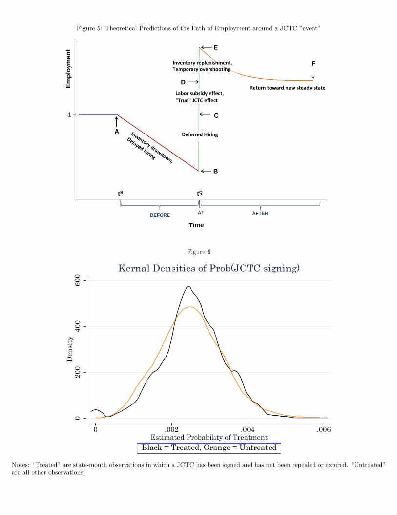
Figure 5: Theoretical Predictions of the Path of Employment around a JCTC ”event”

tS tQ

A

B

C

D

E

F

BEFORE AT AFTER

Empl

oym

ent

Time

Deferred Hiring

Inventory replenishment,Temporary overshooting

Labor subsidy effect,"True" JCTC effect

Return toward new steady‐state

1

Figure 6

020

040

060

0D

ensi

ty

0 .002 .004 .006Estimated Probability of Treatment

Black = Treated, Orange = Untreated

Kernal Densities of Prob(JCTC signing)

Notes: “Treated” are state-month observations in which a JCTC has been signed and has not been repealed or expired. “Untreated”are all other observations.

Table 1: Expected Impacts Of JCTCs On Employment Growth By Regime, By Interval Theoretical Predictions

Regimes Intervals

Before

(1)

At

(2)

After

(3)

Total

(4)

Delayed -

[AD]

++

[CR]

+ or - +

[CUM]

Immediate N/A +

[CR]

+ or - +

[CUM]

Table 2: Summary Statistics Employment Level, Employment Growth, and Legislated JCTCs

Notes: Data for the period January 1990 to December 2010. The data in Panel C are for 21 job creation tax credit adoptions. Employment Level is in thousands. Employment Growth and JCTC values are in percentage points.

State JCTC Status Mean Median Std. Dev. N (1) (2) (3) (4)

A. Employment Level (Thousands)

Delayed-JCTC 1,765.4 1,178.9 1,431.0 1,365

Immediate-JCTC 2,339.2 2,112.4 1,426.2 2,730

No-JCTC 2,243.8 1,295.3 2,695.5 5,222

All 2,201.7 1,497.9 2,236.5 9,317

B. Employment Growth (%, monthly frequency)

Delayed-JCTC 0.132 0.138 0.294 1,365

Immediate-JCTC 0.093 0.110 0.339 2,730

No-JCTC 0.143 0.155 0.313 5,222

All 0.127 0.138 0.319 9,317

C. Legislated JCTCs (% of average state

wage)

Delayed-JCTC 4.274 3.196 2.952 1,170

Immediate-JCTC 11.436 5.000 18.632 1,950

No-JCTC 0 0 0 5,222

All 3.640 0 10.470 8,342

Table 3: JCTC Adoption Decision

Logit Estimator

(1) (2) (3) (4) (5)

Employment growth from t-3 to t -0.000 0.038 -0.014(0.432) (0.479) (0.483)[1.000] [0.937] [0.976]

Employment growth from t-6 to t-3 0.354 0.400 0.275(0.460) (0.464) (0.472)[0.441] [0.388] [0.560]

Employment growth from t-12 to t-6 0.033 0.124 -0.044(0.240) (0.280) (0.333)[0.890] [0.659] [0.895]

Employment Growth from t-24 to t-12 0.127(0.152)[0.403]

Relative employment growth from t-3 to t 0.039 -0.015(0.481) (0.485)[0.935] [0.976]

Relative employment growth from t-6 to t-3 0.401 0.275(0.466) (0.474)[0.389] [0.562]

Relative employment growth from t-12 to t-6 0.126 -0.041(0.282) (0.335)[0.655] [0.902]

Relative Employment Growth from t-24 to t-12 0.127(0.153)[0.405]

COMPETITION 0.003 0.099 0.099 0.096 0.096(0.008) (0.037) (0.037) (0.039) (0.039)[0.708] [0.007] [0.007] [0.014] [0.014]

CORPORATE INCOME TAX RATE (CITR) 0.076 -1.396 -1.396 -1.318 -1.319(0.081) (0.895) (0.896) (0.896) (0.896)[0.350] [0.119] [0.119] [0.141] [0.141]

REPUBLICAN -0.370 1.482 1.484 1.652 1.653(0.610) (1.245) (1.244) (1.281) (1.281)[0.545] [0.234] [0.233] [0.197] [0.197]

Joint Significance of emp growth lags (p-value) 0.694 0.630 0.630 0.861 0.862Observations 8349 2151 2151 1899 1899

Notes: Cells show coefficient, std. error (in parentheses), and p-value [in brackets]. Statefixed effects are excluded from the model in Column (1) but included in the models inColumns (2)-(5).

Table 4: Effects of JCTCs on Employment Growth by Regime and IntervalAlternative AFTER LengthsATE-IPW EstimatorJCTC Measured By Indicator Variable

AFTER = 12m AFTER = 24m AFTER = 36m

Delayed Immediate Delayed Immediate Delayed Immediate

Before -0.068 0.000 -0.065 0.000 -0.062 0.000

(0.025) (0.000) (0.026) (0.000) (0.025) (0.000)

[0.006] [0.000] [0.014] [0.000] [0.014] [0.000]

At 0.141 0.036 0.145 0.037 0.147 0.040

(0.053) (0.038) (0.053) (0.038) (0.053) (0.038)

[0.007] [0.341] [0.006] [0.326] [0.006] [0.302]

After -0.010 0.020 0.025 0.020 0.032 0.027

(0.031) (0.014) (0.019) (0.014) (0.015) (0.010)

[0.755] [0.158] [0.178] [0.149] [0.026] [0.010]

Cumulative Effect (CUM) -0.325 0.277 0.411 0.505 0.992 1.003

(0.340) (0.183) (0.500) (0.333) (0.525) (0.391)

[0.339] [0.130] [0.411] [0.129] [0.059] [0.010]

Number of JCTCs 7 14 7 14 7 14

Notes: Cells show coefficient, standard error (in parentheses), and p-value [in brackets].The cell entries for the BEFORE, AT, and AFTER intervals measure the effects on em-ployment growth per month. The Cumulative Effect sums the product of each interval’scoefficient and the number of months in that interval for either the delayed or immediateregime. Each model includes Two-Way Fixed Effects And Controls.

Table 5: Effects of JCTCs on Employment Growth by Regime and IntervalAlternative AFTER LengthsATE-IPW EstimatorJCTC Measured by Pecuniary Credit Rate Variable

AFTER = 12m AFTER = 24m AFTER = 36m

Delayed Immediate Delayed Immediate Delayed Immediate

Before -1.425 0.000 -1.305 0.000 -1.311 0.000

(0.408) (0.000) (0.418) (0.000) (0.399) (0.000)

[0.000] [0.000] [0.002] [0.000] [0.001] [0.000]

At 1.208 0.159 1.311 0.364 1.307 0.366

(1.516) (0.707) (1.513) (0.692) (1.528) (0.694)

[0.426] [0.822] [0.386] [0.599] [0.392] [0.598]

After -0.515 -1.020 0.692 0.505 0.444 0.351

(0.458) (0.334) (0.313) (0.309) (0.199) (0.369)

[0.260] [0.002] [0.027] [0.102] [0.026] [0.341]

Cumulative Effect (CUM) -12.813 -12.084 10.749 12.481 10.066 13.015

(5.216) (4.220) (8.021) (7.383) (7.069) (13.302)

[0.014] [0.004] [0.180] [0.091] [0.154] [0.328]

Number of JCTCs 6 10 6 10 6 10

Notes: See Table 4 notes. γBEFOREDel is multiplied by -1 to maintain comparability with

Table 4 (see text for details).

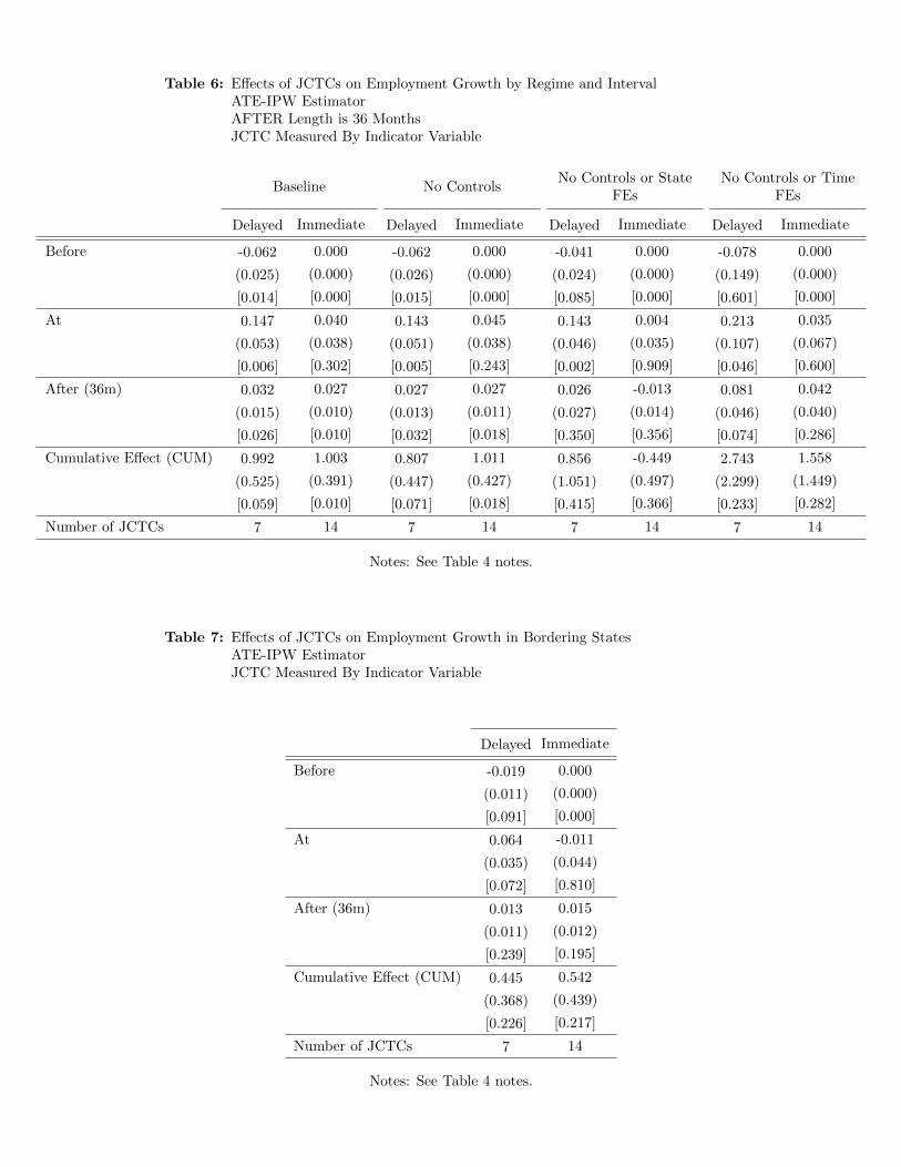
Table 6: Effects of JCTCs on Employment Growth by Regime and IntervalATE-IPW EstimatorAFTER Length is 36 MonthsJCTC Measured By Indicator Variable

Baseline No ControlsNo Controls or State

FEsNo Controls or Time

FEs

Delayed Immediate Delayed Immediate Delayed Immediate Delayed Immediate

Before -0.062 0.000 -0.062 0.000 -0.041 0.000 -0.078 0.000

(0.025) (0.000) (0.026) (0.000) (0.024) (0.000) (0.149) (0.000)

[0.014] [0.000] [0.015] [0.000] [0.085] [0.000] [0.601] [0.000]

At 0.147 0.040 0.143 0.045 0.143 0.004 0.213 0.035

(0.053) (0.038) (0.051) (0.038) (0.046) (0.035) (0.107) (0.067)

[0.006] [0.302] [0.005] [0.243] [0.002] [0.909] [0.046] [0.600]

After (36m) 0.032 0.027 0.027 0.027 0.026 -0.013 0.081 0.042

(0.015) (0.010) (0.013) (0.011) (0.027) (0.014) (0.046) (0.040)

[0.026] [0.010] [0.032] [0.018] [0.350] [0.356] [0.074] [0.286]

Cumulative Effect (CUM) 0.992 1.003 0.807 1.011 0.856 -0.449 2.743 1.558

(0.525) (0.391) (0.447) (0.427) (1.051) (0.497) (2.299) (1.449)

[0.059] [0.010] [0.071] [0.018] [0.415] [0.366] [0.233] [0.282]

Number of JCTCs 7 14 7 14 7 14 7 14

Notes: See Table 4 notes.

Table 7: Effects of JCTCs on Employment Growth in Bordering StatesATE-IPW EstimatorJCTC Measured By Indicator Variable

Delayed Immediate

Before -0.019 0.000

(0.011) (0.000)

[0.091] [0.000]

At 0.064 -0.011

(0.035) (0.044)

[0.072] [0.810]

After (36m) 0.013 0.015

(0.011) (0.012)

[0.239] [0.195]

Cumulative Effect (CUM) 0.445 0.542

(0.368) (0.439)

[0.226] [0.217]

Number of JCTCs 7 14

Notes: See Table 4 notes.

Table 8: Cost Per Job Created

Delayed Regime

Immediate Regime

All JCTC States

(1) (2) (3)

Total Cost Per Job $13,213 $16,644 $16,070

Marginal Subsidy $2,159 (16%)

$4,029 (24%)

$3,328 (21%)

Inframarginal Subsidy $11,054 (84%)

$12,615 (76%)

$12,742 (79%)

Notes: The dollar values in each column are based on equation (27) in the text and using average values for that regime (Delayed-JCTC states, Immediate-JCTC states, and all JCTC states) for each component in that equation.