This is “Cost and Production”, chapter 4 from the book Managerial Economics Principles (index.html) (v. 1.0).

This book is licensed under a Creative Commons by-nc-sa 3.0 (http://creativecommons.org/licenses/by-nc-sa/3.0/) license. See the license for more details, but that basically means you can share this book as long as youcredit the author (but see below), don't make money from it, and do make it available to everyone else under thesame terms.

This content was accessible as of December 29, 2012, and it was downloaded then by Andy Schmitz(http://lardbucket.org) in an effort to preserve the availability of this book.

Normally, the author and publisher would be credited here. However, the publisher has asked for the customaryCreative Commons attribution to the original publisher, authors, title, and book URI to be removed. Additionally,per the publisher's request, their name has been removed in some passages. More information is available on thisproject's attribution page (http://2012books.lardbucket.org/attribution.html?utm_source=header).

For more information on the source of this book, or why it is available for free, please see the project's home page(http://2012books.lardbucket.org/). You can browse or download additional books there.

i

Chapter 4

Cost and Production

In the previous two chapters we examined the economics underlying decisionsrelated to which goods and services a business concern will sell, where it will sellthem, how it will sell them, and in what quantities. Another challenge formanagement is to determine how to acquire and organize its production resourcesto best support those commitments. In this chapter and in the following chapter wewill be discussing key concepts and principles from microeconomics that guide itsorganization and production activities to improve profitability and be able tocompete effectively.

A number of highly useful methodologies have been developed based on theconcepts and principles discussed. This text will not address specific techniques fortracking costs and planning production activities. Readers seeking guidance onthese tasks might consult a text on cost accounting or operations management.Twoclassic texts on cost accounting and operations management are by Horngren(1972) and Stevenson (1986), respectively.

51

4.1 Average Cost Curves

In Chapter 2 "Key Measures and Relationships", we cited average cost as a keyperformance measure in producing a good or service. Average cost reflects the coston a per unit basis. A portion of the average cost is the amount of variable costs thatcan be assigned to the production unit. The other portion is the allocation of fixedcosts (specifically those fixed costs that are not sunk), apportioned to eachproduction unit.

The average cost generally varies as a function of the production volume perperiod. Since fixed costs do not increase with quantity produced, at least in theshort run where production capabilities are relatively set, the portion of theaverage cost attributable to fixed cost is very high for small production volume butdeclines rapidly and then levels off as the volume increases.

The portion of average cost related to the variable cost usually changes lessdramatically in response to production volume than the average fixed cost. In fact,in the example of the ice cream bar business in Chapter 2 "Key Measures andRelationships", we assumed the average variable cost of an ice cream bar wouldremain $0.30 per unit whether the operation sold a small volume or large volume ofice cream bars. However, in actual production environments, average variable costmay fluctuate with volume.

At very low production volumes, resources may not be used efficiently, so thevariable cost per unit is higher. For example, suppose the ice cream bar ventureoperators purchase those bars wholesale from a vendor who delivers them in atruck with a freezer. Since the vendor’s charge for ice cream bars must cover thecost of the truck driver and truck operation, a large delivery that fills the truck islikely to cost less per ice cream bar than a very small delivery.

At the same time, pushing production levels to the upper limits of an operation’scapability can result in other inefficiencies and cause the average variable cost toincrease. For example, in order to increase production volume in a factory, it maybe necessary to pay workers to work overtime at a rate 1.5 times their normal payrate. Another example is that machines may be overworked to drive higher volumebut result in either less efficiency or higher maintenance cost, which translates intoan increase in average variable cost.

Figure 4.1 "Breakdown of Average Cost Function Into Variable Cost and Fixed CostComponent" shows a general breakdown of average cost into average fixed cost and

Chapter 4 Cost and Production

52

average variable cost. The figure reflects the earlier situations of variable costinefficiencies at very low and very high production volumes. Note that even withthe continued decline in the average fixed cost, there is a production level (markedQ*) where the average total cost is at its lowest value. Economists called theproduction volume where average cost is at the lowest value the capacity1 of theoperation.

In conversational language, we often think of capacity of a container as themaximum volume the container can hold. In that sense of the word, it seemsawkward to call the production level Q* the capacity when the graph indicates thatit is possible to produce at higher volume levels but just that the average cost perunit will be higher. However, even in physics, the volume in a container can bechanged by the use of pressure or temperature, so volume is not limited by thecapacity under normal pressures and temperatures.

Figure 4.1 Breakdown of Average Cost Function Into Variable Cost and Fixed Cost Component

The production level corresponding to the lowest point on the graph for average cost indicates the short-runcapacity of the business operation.

In the economic sense of the word, we might think of capacity as the volume levelwhere we have the most efficient operation in terms of average cost. Many

1. The production volume whereaverage cost is at the lowestvalue; the volume level where abusiness has the most efficientoperation in terms of averagecost.

Chapter 4 Cost and Production

4.1 Average Cost Curves 53

businesses can operate over capacity, up to some effective physical limit, but in sodoing will pay for that supplemental production volume in higher costs, due toneeding to employ either more expensive resources or less productive resources,creating congestion that slows production, or overusing resources that results inhigher maintenance costs per unit.

If the price earned by the business at these overcapacity volumes is sufficientlyhigh, the firm may realize more profit by operating over capacity than at thecapacity point where total average cost is at its lowest. Similarly, if demand is weakand customers will pay a price well in excess of average cost only at volumes lowerthan capacity, the firm will probably do better by operating below capacity.However, if a firm that is operating well above capacity or well below capacity doesnot see this as a temporary situation, the discrepancy suggests that the firm is sizedeither too small or too large. The firm may be able to improve profits in futureproduction periods by resizing its operations, which will readjust the capacitypoint. If the firm operates in a very competitive market, there may even be littlepotential for profit for firms that are not operating near their capacity level.

Chapter 4 Cost and Production

4.1 Average Cost Curves 54

4.2 Long-Run Average Cost and Scale

In the last chapter, we distinguished short-run demand from long-run demand toreflect the range of options for consumers. In the short run, consumers werelimited in their choices by their current circumstances of lifestyles, consumptiontechnologies, and understanding. A long-run time frame was of sufficient lengththat the consumer had the ability to alter her lifestyle and technology and toimprove her understanding, so as to result in improved utility of consumption.

There is a similar dichotomy of short-run production decisions and long-runproduction decisions for businesses. In the short run, businesses are somewhatlimited by their facilities, skill sets, and technology. In the long run, businesses havesufficient time to expand, contract, or modify facilities. Businesses can addemployees, reduce employees, or retrain or redeploy employees. They can changetechnology and the equipment used to carry out their businesses.

The classification of short-run planning is more an indication of some temporaryconstraint on redefining the structure of a firm rather than a period of a specificlength. In fact, there are varying degrees of short run. In a very brief period, say thecoming week or month, there may be very little that most businesses can do. It willtake at least that long to make changes in employees and they probably havecontractual obligations to satisfy. Six months may be long enough to changeemployment structures and what supplies a firm uses, but the company is probablystill limited to the facilities and technology they are using.

How long a period is needed until decisions are long term varies by the kind oforganization or industry. A retail outlet might easily totally redefine itself in amatter of months, so for them any decisions going out a year or longer areeffectively long-term decisions. For electricity power generators, it can take 20years to plan, get approvals, and construct a new power generation facility, andtheir long-term period can be in terms of decades.

One important characteristic that distinguishes short-run production2 decisionsand long-run production decisions is in the nature of costs. In the short run, thereare fixed costs and variable costs. However, in the long run, since the firm has theflexibility to change anything about its operations (within the scope of what istechnologically possible and they can afford), all costs in long-run production3

decisions can be regarded as variable costs.

2. A time frame that occurs soonenough that businesses, whichare limited by their facilities,skill sets, and technology,cannot respond by changingtheir production capacity; atime frame in which there arefixed costs and variable costs.

3. A time frame that occurs farenough in the future thatbusinesses have sufficient timeto expand, contract, orotherwise modify theirproduction capacity; a timeframe during which all costsare variable.

Chapter 4 Cost and Production

55

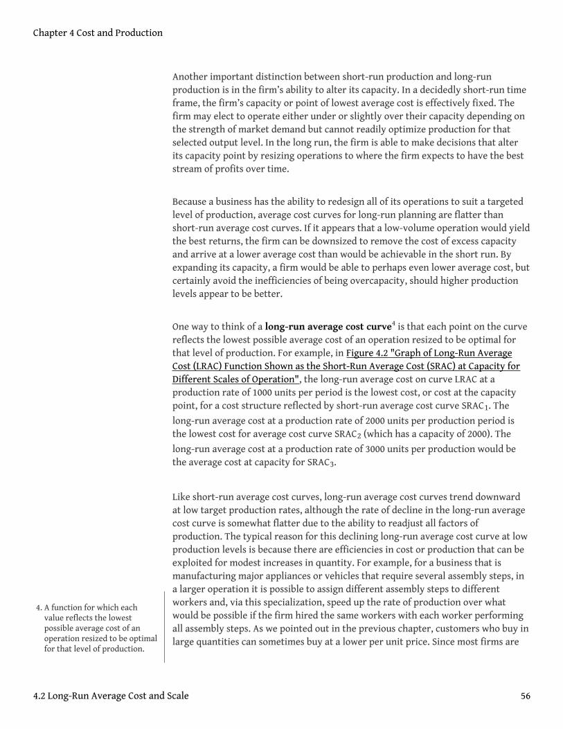
Another important distinction between short-run production and long-runproduction is in the firm’s ability to alter its capacity. In a decidedly short-run timeframe, the firm’s capacity or point of lowest average cost is effectively fixed. Thefirm may elect to operate either under or slightly over their capacity depending onthe strength of market demand but cannot readily optimize production for thatselected output level. In the long run, the firm is able to make decisions that alterits capacity point by resizing operations to where the firm expects to have the beststream of profits over time.

Because a business has the ability to redesign all of its operations to suit a targetedlevel of production, average cost curves for long-run planning are flatter thanshort-run average cost curves. If it appears that a low-volume operation would yieldthe best returns, the firm can be downsized to remove the cost of excess capacityand arrive at a lower average cost than would be achievable in the short run. Byexpanding its capacity, a firm would be able to perhaps even lower average cost, butcertainly avoid the inefficiencies of being overcapacity, should higher productionlevels appear to be better.

One way to think of a long-run average cost curve4 is that each point on the curvereflects the lowest possible average cost of an operation resized to be optimal forthat level of production. For example, in Figure 4.2 "Graph of Long-Run AverageCost (LRAC) Function Shown as the Short-Run Average Cost (SRAC) at Capacity forDifferent Scales of Operation", the long-run average cost on curve LRAC at aproduction rate of 1000 units per period is the lowest cost, or cost at the capacitypoint, for a cost structure reflected by short-run average cost curve SRAC1. The

long-run average cost at a production rate of 2000 units per production period isthe lowest cost for average cost curve SRAC2 (which has a capacity of 2000). The

long-run average cost at a production rate of 3000 units per production would bethe average cost at capacity for SRAC3.

Like short-run average cost curves, long-run average cost curves trend downwardat low target production rates, although the rate of decline in the long-run averagecost curve is somewhat flatter due to the ability to readjust all factors ofproduction. The typical reason for this declining long-run average cost curve at lowproduction levels is because there are efficiencies in cost or production that can beexploited for modest increases in quantity. For example, for a business that ismanufacturing major appliances or vehicles that require several assembly steps, ina larger operation it is possible to assign different assembly steps to differentworkers and, via this specialization, speed up the rate of production over whatwould be possible if the firm hired the same workers with each worker performingall assembly steps. As we pointed out in the previous chapter, customers who buy inlarge quantities can sometimes buy at a lower per unit price. Since most firms are

4. A function for which eachvalue reflects the lowestpossible average cost of anoperation resized to be optimalfor that level of production.

Chapter 4 Cost and Production

4.2 Long-Run Average Cost and Scale 56

buyers as well as sellers, and larger firms will buy in larger quantities, they canreduce the contribution of acquired parts and materials to the average cost.

Figure 4.2 Graph of Long-Run Average Cost (LRAC) Function Shown as the Short-Run Average Cost (SRAC) atCapacity for Different Scales of Operation

The ability to reduce long-run average cost due to increased efficiencies inproduction and cost will usually eventually subside. The production level at whichthe long-run average cost curve flattens out is called the minimum efficient scale5.(Since the business is able to adjust all factors of production in the long run, it caneffectively rescale the entire operation, so the target production level is sometimescalled the scale6 of the business.) In competitive seller markets, the ability of a firmto achieve minimum efficient scale is crucial to its survival. If one firm is producingat minimum efficient scale and another firm is operating below minimum efficientscale, it is possible for the larger firm to push market prices below the cost of thesmaller firm, while continuing to charge a price that exceeds its average cost.Facing the prospect of sustained losses, the smaller firm usually faces a choicebetween getting larger or dropping out of the market.

The increase in capacity needed to achieve minimum efficient scale varies by thetype of business. A bicycle repair shop might achieve minimum efficient scale witha staff of four or five employees and be able to operate at an average cost that is no

5. The production level at whichthe long-run average costcurve flattens out.

6. The target production levelwhen a business is able toadjust all factors of productionin the long run.

Chapter 4 Cost and Production

4.2 Long-Run Average Cost and Scale 57

different than a shop of 40 to 50 repair persons. At the other extreme, electricitydistribution services and telephone services that have very large fixed asset costsand low variable costs may see the long-run average cost curve decline even forlarge production levels and therefore would have a very high minimum efficientscale.

Most firms have a long-run average cost curve that declines and then flattens out;however, in some markets the long-run average cost may actually rise after somepoint. This phenomenon often indicates a limitation in some factors of productionor a decline in quality in factors of production if the scale increases enough. Forexample, in agriculture some land is clearly better suited to certain crops thanother land. In order to match the yield of the best acreage on land of lower quality,it may be necessary to spend more on fertilizer, water, or pest control, therebyincreasing the average cost of production for all acreage used.

Businesses that are able to lower their average costs by increasing the scale of theiroperation are said to have economies of scale7. Firms that will see their averagecosts increase if they further increase their scale will experience diseconomies ofscale8. Businesses that have achieved at least their minimum efficient scale andwould see the long-run average cost remain about the same with continuedincreases in scale may be described as having constant economies of scale9.

The impact of an increase of scale on production is sometimes interpreted in termsof “returns to scale.” The assessment of returns to scale is based on the response tothe following question: If all factors of production (raw materials, labor, energy,equipment time, etc.) where increased by a set percentage (say all increased by10%), would the percent increase in potential quantity of output created be greater,the same, or less than the percent increase in all factors of production? If potentialoutput increases by a higher percent, operations are said to have increasing returnsto scale. If output increases by the same percent, the operations show constantreturns to scale. If the percent growth in outputs is less than the percent increase ininputs used, there are decreasing returns to scale.

Returns to scale are related to the concept of economies of scale, yet there is asubtle difference. The earlier example of gained productivity of labor specializationwhen the labor force is increased would contribute to increasing returns to scale.Often when there are increasing returns to scale there are economies of scalebecause the higher rate of growth in output translates to decrease in average costper unit. However, economies of scale may occur even if there were constantreturns to scale, such as if there were volume discounts for buying supplies inlarger quantities. Economies of scale mean average cost decreases as the scaleincreases, whereas increasing returns to scale are restricted to the physical ratio

7. A situation in which a businesscan lower its average costs byincreasing the size of itsoperation.

8. A situation in which a businessexperiences an increase inaverage costs if it increases thesize of its operation.

9. A situation in which a businessthat has achieved its leastminimum efficient scale seesits long-run average costremain about the same withcontinued increases in the sizeof its operation.

Chapter 4 Cost and Production

4.2 Long-Run Average Cost and Scale 58

between the increase in units of output relative to proportional increase in thenumber of inputs used.

Likewise, decreasing returns to scale often translate to diseconomies of scale. Ifincreasing the acreage used for a particular crop by using less productive acreageresults in a smaller increase in yield than increase in acreage, there are decreasingreturns to scale. Unless the acreage costs less to use, there will be an increase inaverage cost per unit of crop output, indicating diseconomies of scale.

Chapter 4 Cost and Production

4.2 Long-Run Average Cost and Scale 59

4.3 Economies of Scope and Joint Products

Most businesses provide multiple goods and services; in some cases, the number ofgoods and services is quite large. Whereas the motivation for providing multipleproducts may be driven by consumer expectations, a common attraction is theopportunity to reduce per unit costs. When a venture can appreciate such costsavings, the opportunity is called an economy of scope10.

Of course, not just any aggregation of goods and services will create economies ofscope. For significant economies of scope, the goods and services need to be similarin nature or utilize similar raw materials, facilities, production processes, orknowledge.

One type of cost savings is the ability to share fixed costs across the product andservice lines so that the total fixed costs are less than if the operations wereorganized separately. For example, suppose we have a company that expands fromselling one product to two similar products. The administrative functions forprocurement, receiving, accounts payable, inventory management, shipping, andaccounts receivable in place for the first product can usually support the secondproduct with just a modest increase in cost.

A second type of cost savings occurs from doing similar activities in larger volumeand reducing per unit variable costs. If multiple goods and services require thesame raw materials, the firm may be able to acquire the raw materials at a smallerper unit cost by purchasing in larger volume. Similarly, labor that is directly relatedto variable cost may not need to be increased proportionally for additional productsdue to the opportunity to exploit specialization or better use of idle time.

In some cases, two or more products may be natural by-products of a productionprocess. For example, in refining crude oil to produce gasoline to fuel cars andtrucks, the refining process will create lubricants, fertilizers, petrochemicals, andother kinds of fuels. Since the refining process requires heat, the excess heat can beused to create steam for electricity generation that more than meets the refinery’sneeds and may be sold to an electric utility. When multiple products occur at theresult of a combined process, they are called joint products11 and create a naturalopportunity for an economy of scope.

As with economies of scale, the opportunities for economies of scope generallydissipate after exploiting the obvious combinations of goods and services. At somepoint, the complexity of trying to administer a firm with too many goods and

10. The ability of a businessventure to achieve cost savingsby providing multiple goodsand services.

11. The result of a combinedproduction process thatcreates a natural opportunityfor an economy of scope.

Chapter 4 Cost and Production

60

services will offset any cost savings, particularly if the goods and services sharelittle in terms of production resources or processes. However, sometimes firmsdiscover scope economies that are not so obvious and can realize increasedeconomic profits, at least for a time until the competition copies their discovery.

Chapter 4 Cost and Production

4.3 Economies of Scope and Joint Products 61

4.4 Cost Approach Versus Resource Approach to Production Planning

The conventional approach to planning production is to start with the goods andservices that a firm intends to provide and then decide what productionconfiguration will achieve the intended output at the lowest cost. This is the costapproach12 to production planning.Stevenson (1986) addresses this approach toproduction planning extensively. Once output goals are set, the expected revenue isessentially determined, so any remaining opportunity for profit requires reducingthe cost as much as possible.

Although this principle of cost minimization is simple, actually achieving trueminimization in practice is not feasible for most ventures of any complexity.Rather, minimization of costs is a target that is not fully realized because the rangeof production options is wide and the actual resulting costs may differ from whatwas expected in the planning phase.

Additionally, as we saw in Chapter 2 "Key Measures and Relationships", the decisionabout whether to provide a good or service and how much to provide requires anassessment of marginal cost. Due to scale effects, this marginal cost may vary withthe output level, so firms may face a circular problem of needing to know themarginal cost to decide on the outputs, but the marginal cost may changedepending on the output level selected. This dilemma may be addressed by iterationbetween output planning and production/procurement planning until there isconsistency. Another option is to use sophisticated computer models thatdetermine the optimal output levels and minimum cost production configurationssimultaneously.

Among the range of procurement and production activities that a business conductsto create its goods and services, the firm may be more proficient or expert in someof the activities, at least relative to its competition. For example, a firm may beworld class in factory production but only about average in the cost effectiveness ofits marketing activities. In situations where a firm excels in some components of itsoperations, there may be an opportunity for improved profitability by recognizingthese key areas, sometimes called core competencies13 in the business strategyliterature, and then determining what kinds of goods or services would best exploitthese capabilities. This is the resource approach14 to the planning ofproduction.Wernerfelt (1984) wrote one of the key initial papers on the resource-based view of management.

12. Starting with the goods andservices a firm intends toprovide and then decidingwhat configuration will achieveoutput at the lowest cost.

13. Key areas or components ofoperation in which a firmexcels and that provide anopportunity for improvedprofitability.

14. The recognition of corecompetencies and thedetermination of what kinds ofgoods or services best exploitthem.

Chapter 4 Cost and Production

62

Conceptually, either planning approach will lead to similar decisions about whatgoods and services to provide and how to arrange production to do that. However,given the wide ranges of possible outputs and organizations of production toprovide them, firms are not likely to attain truly optimal organization, particularlyafter the fact. The cost approach is often easier to conduct, particularly for a firmthat is already in a particular line of business and can make incrementalimprovements to reduce cost. However, in solving the problem of how to create thegoods and services at minimal cost, there is some risk of myopic focus thatdismisses opportunities to make the best use of core competencies. The resourceapproach encourages more out-of-the-box thinking that may lead a business towarda major restructuring.

Chapter 4 Cost and Production

4.4 Cost Approach Versus Resource Approach to Production Planning 63

4.5 Marginal Revenue Product and Derived Demand

In Chapter 2 "Key Measures and Relationships", we discussed the principle forprofit maximization stating that, absent constraints on production, the optimaloutput levels for the goods and services occur when marginal revenue equalsmarginal cost. This principle can be applied in determining the optimal level of anyproduction resource input using the concepts of marginal product and marginalrevenue product.

The marginal product15 of a production input is the amount of additional outputthat would be created if one more unit of the input were obtained and processed.For example, if an accounting firm sells accountant time as a service and each hiredaccountant is typically billed to clients 1500 hours per year, this quantity would bethe marginal product of hiring an additional accountant.

The marginal revenue product16 of a production input is the marginal revenuecreated from the marginal product resulting from one additional unit of the input.The marginal revenue product would be the result of multiplying the marginalproduct of the input times the marginal revenue of the output. For the example inthe previous paragraph, suppose that at the current output levels, the marginalrevenue from an additional billed hour of accountant service is $100. The marginalrevenue product of an additional accountant would be 1500 times $100, or $150,000.

In determining if a firm is using the optimal level on an input17, the marginalrevenue product for an additional unit of input can be compared to the marginalcost of a unit of the input. If the marginal revenue product exceeds the marginalinput cost, the firm can improve profitability by increasing the use of that inputand the resulting increase in output. If the marginal cost of the input exceeds themarginal revenue product, profit will improve by decreasing the use of that inputand the corresponding decrease in output. At the optimal level, the marginalrevenue product and marginal cost of the input would be equal.

Suppose the marginal cost to hire an additional accountant in the previous examplewas $120,000. The firm would improve its profit by $30,000 by hiring one moreaccountant.

As noted earlier in the discussion of marginal revenue, the marginal revenue willchange as output is increased, usually declining as output levels increase.Correspondingly, the marginal revenue product will generally decrease as the inputand corresponding output continue to be increased. This phenomenon is called the

15. The amount of additionaloutput that would begenerated if one more unit ofan input were obtained andprocessed.

16. The additional revenue createdfrom one additional unit of aninput; the marginal product ofthe input times the marginalrevenue of the output.

17. If the marginal revenueproduct exceeds the marginalinput cost, a firm can improveprofitability by increasing theuse of the input; if themarginal cost of the inputexceeds the marginal revenueproduct, profit can beimproved by decreasing use ofthe input.

Chapter 4 Cost and Production

64

law of diminishing marginal returns to an input18. So, for the accounting firm,although they may realize an additional $30,000 in profit by hiring one moreaccountant, that does not imply they would realize $3,000,000 more in profits byhiring 100 more accountants.

If the marginal revenue product is measured at several possible input levels andgraphed, the pattern suggests a relationship between quantity of input andmarginal revenue product, as shown in Figure 4.3 "Typical Pattern of a DerivedDemand Curve Relating the Marginal Revenue Product to Quantity of InputEmployed in Production". Due to the law of diminishing marginal returns, thisrelationship will generally be negative. Thus the relationship looks much like thedemand curve corresponding to output levels. In fact, this relationship is atransformation of the firm’s demand curve, expressed in terms of the equivalentmarginal revenue product relative to number of units of input used. Due to theconnection to the demand curve for output, the relationship depicted in Figure 4.3"Typical Pattern of a Derived Demand Curve Relating the Marginal Revenue Productto Quantity of Input Employed in Production" is called a derived demand curve19.

Figure 4.3 Typical Pattern of a Derived Demand Curve Relating the Marginal Revenue Product to Quantity ofInput Employed in Production

One difficulty in comparing marginal revenue product to the marginal cost of aninput is that the mere increase in any single input is usually not enough in itself tocreate more units of output. For example, simply acquiring more bicycle frames will

18. Marginal revenue product willdecrease as an input andcorresponding output continueto be increased.

19. A negative relationshipbetween quantity of input andmarginal revenue product thatis a transformation of a firm'sdemand curve.

Chapter 4 Cost and Production

4.5 Marginal Revenue Product and Derived Demand 65

not result in the ability to make more bicycles, unless the manufacturer acquiresmore wheels, tires, brakes, seats, and such to turn those frames into bicycles. Incases like this, sometimes the principle needs to be applied to a fixed mix of inputsrather than a single input.

For the accounting firm in the earlier example, the cost to acquire an additionalaccountant is not merely the salary he is paid. The firm will pay for benefits likeretirement contribution and health care for the new employee. Further, additionalinputs in the form of an office, computer, secretarial support, and such will beincurred. So the fact that the marginal revenue product of an accountant is$150,000 does not mean that the firm would benefit if the accountant were hired atany salary less than $150,000. Rather, it would profit if the additional cost of salary,benefits, office expense, secretarial support, and so on is less than $150,000.

Chapter 4 Cost and Production

4.5 Marginal Revenue Product and Derived Demand 66

4.6 Marginal Cost of Inputs and Economic Rent

In cases where inputs are in high supply at the current market price and the marketfor inputs is competitive, the marginal cost of an input is roughly equal to theactual cost of acquiring it. So, in such a situation, the principle described earlier canbe expressed in terms of comparing the marginal revenue product to price toacquire the input(s). If the number of accountants seeking a job were fairlysubstantial and competitive, the actual per unit costs involved in hiring one moreaccountant would be the marginal cost.

If the market of inputs is less competitive, a firm may have to pay a little higherthan the prevailing market price to acquire more units because they will need to behired away from another firm. In this situation, the marginal cost of inputs may behigher than the price to acquire an additional unit because the resulting priceincrease for the additional unit may carry over to a price increase of all units beingpurchased.

Suppose the salary required to hire a new accountant will be higher than what thefirm is currently paying accountants with the same ability. Once the firm pays ahigher salary to get a new accountant, they may need to raise the salaries of theother similar accountants they already hired just to retain them. In this instance,the marginal cost of hiring one more accountant could be substantially more thanthe cost directly associated with adding the new accountant. As a result of theimpact on other salaries and associated costs of the hire, the firm may decide thatthe highest salary for a new accountant that the firm can justify may be on theorder of $50,000, even though the resulting marginal revenue product issubstantially greater.

If inputs are available in a ready supply, or there are close substitutes available thatare in ready supply, the price of an additional unit of input typically reflects eitherthe opportunity cost related to the value of the next best use of that input or theminimum amount needed to induce a new unit to become available. However, thereare some production inputs that may be in such limited supply that even furtherprice increases will not attract new units to become available, at least not quickly.In these cases, the marginal revenue product for an input may still considerablyexceed its marginal cost, even after all available inputs are in use. The sellers ofthese goods and services may be aware of this imbalance and insist on a priceincrease for the input up to a level that brings marginal cost in balance withmarginal revenue product. The difference between the amount the provider of thelimited input supply is able to charge and the minimum amount that would have

Chapter 4 Cost and Production

67

been necessary to induce the provider to sell the unit to the firm is called economicrent20.

Suppose a contracting firm was hired to do emergency repairs to a major bridge.Due to the time deadline, the firm will need to hire additional construction workerswho are already in the area. Normally, these workers may have been willing towork for $70 per hour. However, sensing the contracting firm is being paid apremium for the repairs, meaning the marginal revenue product of labor is high,and there are a limited number of qualified workers available, the workers caninsist on being paid as much as $200 per hour for the work. The difference of $130would be economic rent caused by the shortage of qualified workers available onshort notice.

Economic rent can occur in agriculture when highly productive land is in limitedsupply or in some labor markets like professional sports or commercialentertainment where there is a limited supply of people who have the skills orname recognition needed to make the activity successful.

20. The difference between theamount the provider of alimited input supply is able tocharge and the minimumamount that would benecessary to induce theprovider to sell the unit to afirm.

Chapter 4 Cost and Production

4.6 Marginal Cost of Inputs and Economic Rent 68

4.7 Productivity and the Learning Curve

The resource view of production management is to make sure that all resourcesemployed in the creation of goods and services are used as effectively as possible.Smart businesses assess the productivity of key production resources as a means oftracking improvements and in comparing their operations to those of other firms.

Earlier in this chapter we introduced the concept of marginal product. Thismeasure reflects how productive an additional unit of that input would be increating additional output. However, for some inputs, there are differences inmarginal productivity across units. For example, in agriculture an acre of land inone location may be capable of better yields than an acre in another location. Atany given input price, firms will seek to employ those units with the highestmarginal product first.

In looking at the collective performance of a production operation, we need ameasure of productivity that applies to all inputs being used rather than the lastunit acquired. One means of doing this is using the measure of averageproductivity21, which is a ratio of the total number of units of output divided by thetotal units of an input. An alternative measure of average productivity would be thetotal dollars in revenue or profit divided by the total units of an input.

Computations of average productivity make sense for key inputs around whichproduction processes are designed. In the example of the accounting firm used inthis chapter, the number of accountants is probably a good choice. Averageproductivity could be in the form of labor hours billed divided by accountantshired. If a firm managed to sell 1600 billable hours in 1 year, but only 1500 billablehours in another year, the earlier year indicated higher productivity.

In retail stores, a key resource is the amount of floor space. The productivity of astore could be measured by the total revenue over a period divided by the availablesquare footage. This measure could be compared to the same measure for otherstores in the retail chain or with similar competitor stores. Even sections within thestore can be compared for which types of goods and services sold are most effectivein generating sales, although given that costs vary too, a better productivitymeasure here may be profit contribution (revenue minus variable cost) per squarefoot.

The productivity of firms may change over time. In the case of labor, theproductivity of individual workers will rise as they gain experience and new

21. The total number of units ofoutput divided by the totalunits of an input; the totaldollars in revenue or profitdivided by the total units of aninput.

Chapter 4 Cost and Production

69

workers can be trained more effectively. There is also an improvement in overallproductivity from the increased knowledge of management in how to employproductive resources better. These productivity gains from experience andimproved knowledge are sometimes called learning by doing22The economics oflearning by doing was introduced by Arrow (1962).

In addition to the increased profit potential of improved productivity, new firms orfirms starting new operations need to anticipate these gains in deciding whether toengage in a new venture. Often a venture will not look attractive if the assumedcosts of production are based on the costs that apply in the initial periods ofproduction. Learning improvements need to be considered as well. In some sense,decreased profits and even losses in the initial production periods are necessaryinvestments for a successful long-term operation.

Improvements due to productivity gains will usually result in decreased averagecosts. The relationship between cumulative production experience and average costis called the learning curve23. An example appears in Figure 4.4 "Pattern of aLearning Curve Showing Average Cost Declining by a Fixed Percentage for EachDoubling of Cumulative Output". One point to be emphasized is that the quantity onthe horizontal axis is cumulative production24, or total production to date, ratherthan production rate per production period. This is not a scale effect per se. Even ifthe firm continues to produce at the same rate each period, it will see declines inthe average cost per unit of output, especially in the initial stages of operation.

One numerical measure of the impact of learning on average cost is called thedoubling rate of reduction25. The doubling rate is the reduction in average costthat occurs each time cumulative production doubles. If the average cost declines by15% each time cumulative production doubles, that would be its doubling rate. Alearning curve with a doubling rate of 15% may be called an 85% learning curve toindicate the magnitude of the average cost compared to when cumulativeproduction was only half as large.

22. Productivity gains that comefrom experience and improvedknowledge.

23. The relationship betweencumulative productionexperience and average cost.

24. Total production to date.

25. The decrease in average costthat occurs each timecumulative productiondoubles.

Chapter 4 Cost and Production

4.7 Productivity and the Learning Curve 70

Figure 4.4 Pattern of a Learning Curve Showing Average Cost Declining by a Fixed Percentage for EachDoubling of Cumulative Output

Note that the number of units required to double cumulative production will getprogressively higher. For example, if cumulative production now is 1000 units, thenext doubling will occur at 2000 cumulative units, with the next doubling at 4000cumulative units, and the following at 8000 cumulative units. Thus the rate ofdecline in average cost for each successive unit of production will diminish ascumulative production increases.

Chapter 4 Cost and Production

4.7 Productivity and the Learning Curve 71