A PROTOTYPE PLATFORM FOR ARRAY FEED

DEVELOPMENT

by

James Richard Nagel

A thesis submitted to the faculty of

Brigham Young University

in partial fulfillment of the requirements for the degree of

Master of Science

Department of Electrical and Computer Engineering

Brigham Young University

December 2006

Copyright c© 2006 James Richard Nagel

All Rights Reserved

BRIGHAM YOUNG UNIVERSITY

GRADUATE COMMITTEE APPROVAL

of a thesis submitted by

James Richard Nagel

This thesis has been read by each member of the following graduate committee andby majority vote has been found to be satisfactory.

Date Karl F. Warnick, Chair

Date Brian D. Jeffs

Date Michael A. Jensen

BRIGHAM YOUNG UNIVERSITY

As chair of the candidate’s graduate committee, I have read the thesis of JamesRichard Nagel in its final form and have found that (1) its format, citations, and bib-liographical style are consistent and acceptable and fulfill university and departmentstyle requirements; (2) its illustrative materials including figures, tables, and chartsare in place; and (3) the final manuscript is satisfactory to the graduate committeeand is ready for submission to the university library.

Date Karl F. WarnickChair, Graduate Committee

Accepted for the Department

Michael J. WirthlinGraduate Coordinator

Accepted for the College

Alan R. ParkinsonDean, Ira A. Fulton College ofEngineering and Technology

ABSTRACT

A PROTOTYPE PLATFORM FOR ARRAY FEED DEVELOPMENT

James Richard Nagel

Department of Electrical and Computer Engineering

Master of Science

Radio frequency interference (RFI) is a growing problem for radio astronomers.

One potential solution utilizes spatial filtering by placing an array of electrically small

antennas at the focal plane of a parabolic reflector. This thesis documents the design

and characterization of a prototype array feed and RF receiver that were used to

demonstrate the spatial filtering principle. The array consists of a 7-element hexag-

onal arrangement of thickened dipole antennas tuned to a center frequency of 1600

MHz. The receiver is a two-stage, low-noise frequency mixer that is tunable over

the entire L-band. This thesis also documents a new receiver design that is part of

an upgrade to the outdoor antenna test range for the National Radio Astronomy

Observatory in Green Bank, West Virginia.

The array feed was demonstrated on a three-meter parabolic reflector by re-

covering a weak signal of interest that was obscured by a strong, broadband interferer.

Similar results were also obtained when the interferer moved with an angular velocity

of 0.1/s, but only when the power in the interferer dominated the signal. Using a

link budget calculation, the aperture efficiency of the receiver was measured at 64%.

A measurement of pattern rumble was also carried out by comparing the SNRs of

adaptive beamformers to the SNR of a fixed-weight beamformer. It was found that

adaptive beamforming on a moving interferer introduces a significant amount of pat-

tern rumble and reduces the maximum integration time by roughly one order of

magnitude.

ACKNOWLEDGMENTS

I would like to extend my gratitude and appreciation to the following individuals.

Dr. Karl Warnick, for recruiting me into the project, for his guidance with

my research, and patience with my learning.

Dr. Brian Jeffs, for his council and advice with my research.

Dr. Rick Fisher and Dr. Richard Bradley, for their support with my work at

the NRAO.

Chris Ashworth, Micah Lilrose, and Jonathon Landon for their assistance on

all of my projects.

Dr. Long and the MERS Lab, for sharing their resources, their time, and

their friendship.

Joe Bussio for his council and assistance with the machine shop.

And of course, my parents, Barbara and David Nagel, for always encouraging

me to work hard, study hard, and aim high.

Table of Contents

Acknowledgements xiii

List of Tables xix

List of Figures xxiii

1 Introduction 1

1.1 Radio Astronomy and RFI . . . . . . . . . . . . . . . . . . . . . . . . 1

1.2 Thesis Contributions . . . . . . . . . . . . . . . . . . . . . . . . . . . 3

1.3 Thesis Outline . . . . . . . . . . . . . . . . . . . . . . . . . . . . . . . 3

2 Array Theory and Beamforming 5

2.1 Array Modeling . . . . . . . . . . . . . . . . . . . . . . . . . . . . . . 5

2.1.1 Directivity . . . . . . . . . . . . . . . . . . . . . . . . . . . . . 6

2.1.2 Hertzian Dipole Model . . . . . . . . . . . . . . . . . . . . . . 7

2.2 Receive Arrays . . . . . . . . . . . . . . . . . . . . . . . . . . . . . . 7

2.2.1 Steering Vectors . . . . . . . . . . . . . . . . . . . . . . . . . . 8

2.3 Correlation Matrix Estimation . . . . . . . . . . . . . . . . . . . . . . 10

2.4 Beamforming . . . . . . . . . . . . . . . . . . . . . . . . . . . . . . . 10

2.4.1 Maximum Gain . . . . . . . . . . . . . . . . . . . . . . . . . . 11

2.4.2 Maximum SINR . . . . . . . . . . . . . . . . . . . . . . . . . . 11

2.4.3 LCMV . . . . . . . . . . . . . . . . . . . . . . . . . . . . . . . 12

2.4.4 Orthogonal Subspace Projection . . . . . . . . . . . . . . . . . 13

2.5 Power Calibration . . . . . . . . . . . . . . . . . . . . . . . . . . . . . 13

xv

3 A Two-Stage Receiver for the Focal-Plane Array 15

3.1 Design Considerations . . . . . . . . . . . . . . . . . . . . . . . . . . 15

3.1.1 RFI Survey . . . . . . . . . . . . . . . . . . . . . . . . . . . . 16

3.1.2 System Overview . . . . . . . . . . . . . . . . . . . . . . . . . 17

3.2 Front-End . . . . . . . . . . . . . . . . . . . . . . . . . . . . . . . . . 17

3.3 Receiver Box . . . . . . . . . . . . . . . . . . . . . . . . . . . . . . . 19

3.3.1 Band-Pass Filter . . . . . . . . . . . . . . . . . . . . . . . . . 19

3.3.2 Amplifier 1 and Mixer 1 . . . . . . . . . . . . . . . . . . . . . 21

3.3.3 IF Stage and Mixer 2 . . . . . . . . . . . . . . . . . . . . . . . 22

3.4 Back-End . . . . . . . . . . . . . . . . . . . . . . . . . . . . . . . . . 24

3.5 DC Power . . . . . . . . . . . . . . . . . . . . . . . . . . . . . . . . . 25

3.6 Summary and Characterization . . . . . . . . . . . . . . . . . . . . . 25

4 The Seven-Element Hexagonal Array 31

4.1 Array Geometry . . . . . . . . . . . . . . . . . . . . . . . . . . . . . . 31

4.2 Element Characterization . . . . . . . . . . . . . . . . . . . . . . . . 31

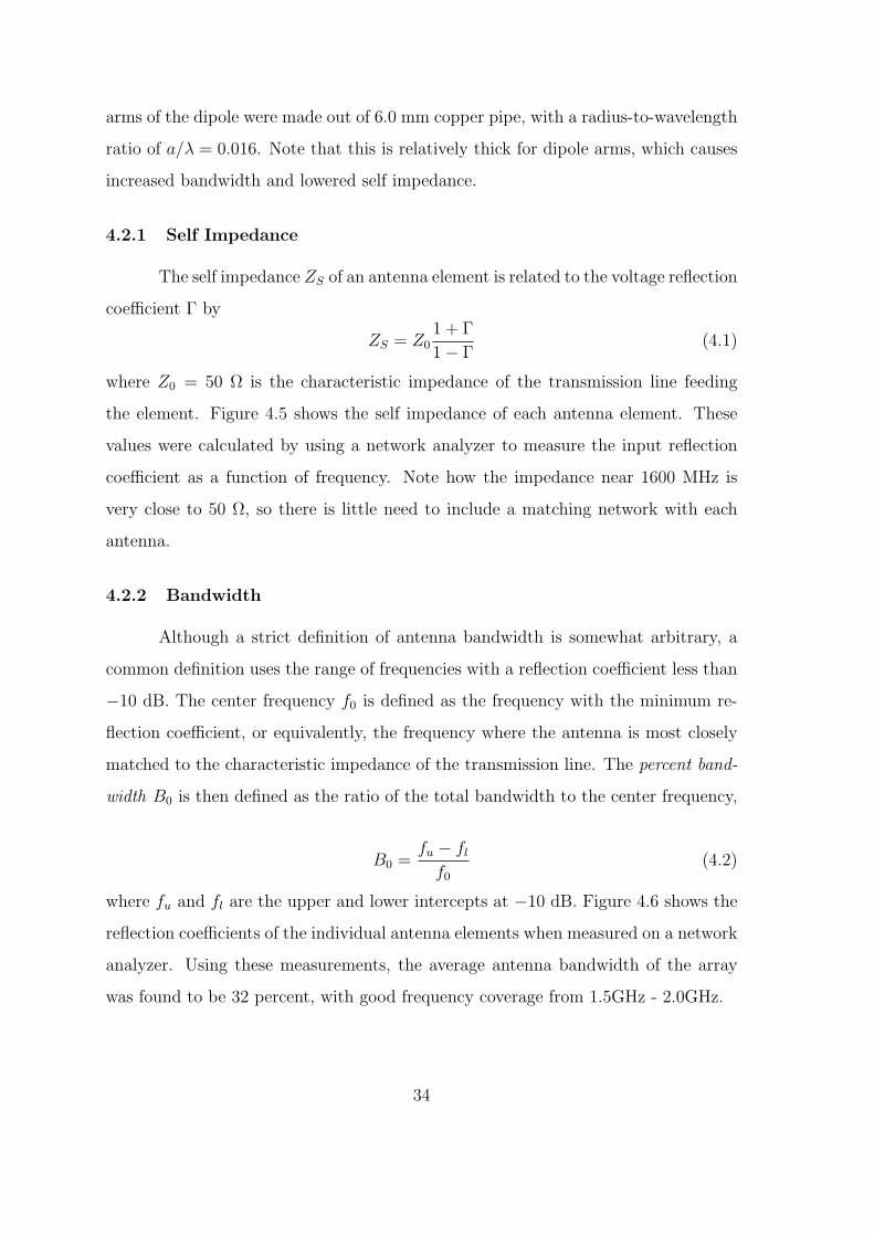
4.2.1 Self Impedance . . . . . . . . . . . . . . . . . . . . . . . . . . 34

4.2.2 Bandwidth . . . . . . . . . . . . . . . . . . . . . . . . . . . . . 34

4.3 Mutual Coupling . . . . . . . . . . . . . . . . . . . . . . . . . . . . . 36

4.4 Gain and Effective Area . . . . . . . . . . . . . . . . . . . . . . . . . 36

5 Antenna Test Range Receiver Design for the NRAO Headquarters 41

5.1 Geometry . . . . . . . . . . . . . . . . . . . . . . . . . . . . . . . . . 41

5.2 The Lock-In Amplifier . . . . . . . . . . . . . . . . . . . . . . . . . . 42

5.3 Theoretical Design Layout . . . . . . . . . . . . . . . . . . . . . . . . 44

5.4 LO Frequency . . . . . . . . . . . . . . . . . . . . . . . . . . . . . . . 44

5.5 Power Losses . . . . . . . . . . . . . . . . . . . . . . . . . . . . . . . 44

5.5.1 Line Loss . . . . . . . . . . . . . . . . . . . . . . . . . . . . . 45

5.5.2 Propagation Loss . . . . . . . . . . . . . . . . . . . . . . . . . 46

5.5.3 Conversion Loss . . . . . . . . . . . . . . . . . . . . . . . . . . 46

5.5.4 Splitter Loss . . . . . . . . . . . . . . . . . . . . . . . . . . . . 46

xvi

5.5.5 Power Budget . . . . . . . . . . . . . . . . . . . . . . . . . . . 46

5.6 Reference Signal Bleed-Through . . . . . . . . . . . . . . . . . . . . . 47

5.7 Bleed-Through Solution . . . . . . . . . . . . . . . . . . . . . . . . . 48

5.8 Reference Input Power . . . . . . . . . . . . . . . . . . . . . . . . . . 49

5.9 Low-Pass Filters . . . . . . . . . . . . . . . . . . . . . . . . . . . . . 49

5.10 Summary . . . . . . . . . . . . . . . . . . . . . . . . . . . . . . . . . 49

5.11 Array Directivity Measurements . . . . . . . . . . . . . . . . . . . . . 50

5.11.1 Calibration . . . . . . . . . . . . . . . . . . . . . . . . . . . . 51

5.11.2 Directivity Results . . . . . . . . . . . . . . . . . . . . . . . . 52

6 RFI Mitigation with the Focal-Plane Array 55

6.1 Experimental Setup . . . . . . . . . . . . . . . . . . . . . . . . . . . . 55

6.2 Calibration and Alignment . . . . . . . . . . . . . . . . . . . . . . . . 58

6.3 Training Data . . . . . . . . . . . . . . . . . . . . . . . . . . . . . . . 58

6.4 Effective Area and Aperture Efficiency . . . . . . . . . . . . . . . . . 59

6.5 Stationary Interferer . . . . . . . . . . . . . . . . . . . . . . . . . . . 60

6.5.1 Single Element . . . . . . . . . . . . . . . . . . . . . . . . . . 60

6.5.2 Max SINR using Interferer Subspace Partitioning . . . . . . . 61

6.6 Non-stationary Interferer . . . . . . . . . . . . . . . . . . . . . . . . . 61

6.6.1 Single Element . . . . . . . . . . . . . . . . . . . . . . . . . . 63

6.6.2 Max SINR using Interferer Subspace Partitioning . . . . . . . 63

6.7 Performance Versus Interferer Power . . . . . . . . . . . . . . . . . . 65

6.8 Correlation Time and Non-Stationarity . . . . . . . . . . . . . . . . . 66

6.9 Pattern Rumble . . . . . . . . . . . . . . . . . . . . . . . . . . . . . . 69

7 Conclusions and Future Work 73

7.1 Robust Beamformers . . . . . . . . . . . . . . . . . . . . . . . . . . . 73

7.2 Array Weight Normalization . . . . . . . . . . . . . . . . . . . . . . . 73

7.3 Optimal Feed Placement . . . . . . . . . . . . . . . . . . . . . . . . . 74

7.4 Mutual Coupling . . . . . . . . . . . . . . . . . . . . . . . . . . . . . 74

7.5 Sensitivity . . . . . . . . . . . . . . . . . . . . . . . . . . . . . . . . . 74

xvii

7.6 Array Expansion . . . . . . . . . . . . . . . . . . . . . . . . . . . . . 74

7.7 Astronomical Observation on the GBT . . . . . . . . . . . . . . . . . 75

Bibliography 79

xviii

List of Tables

3.1 Receiver characterization. . . . . . . . . . . . . . . . . . . . . . . . . 28

3.2 Major parts list and power budget. . . . . . . . . . . . . . . . . . . . 28

3.3 Minor parts list. . . . . . . . . . . . . . . . . . . . . . . . . . . . . . . 29

xix

xx

List of Figures

3.1 RFI survey results. The data was averaged for two minutes on a digital

spectrum analyzer. . . . . . . . . . . . . . . . . . . . . . . . . . . . . 16

3.2 Block diagram for the radio astronomy array-feed receivers. The dashed

boxes indicate the three major sections. . . . . . . . . . . . . . . . . . 18

3.3 Receiver front-end. . . . . . . . . . . . . . . . . . . . . . . . . . . . . 19

3.4 Photograph of the receiver box section with the cover removed. . . . 20

3.5 Block diagram of the receiver box section. Note that each box contains

two channels, labeled A and B. . . . . . . . . . . . . . . . . . . . . . 20

3.6 Frequency response of the low-pass, high-pass filter combination to

form a single band-pass filter. . . . . . . . . . . . . . . . . . . . . . . 21

3.7 SAW filter soldered into the a Mini-Circuits amplifier case. The SAW

is a passive device, so the power leads are left floating. . . . . . . . . 23

3.8 Frequency response of the SAW filter. . . . . . . . . . . . . . . . . . . 23

3.9 Receiver back-end. . . . . . . . . . . . . . . . . . . . . . . . . . . . . 24

3.10 DC-DC regulator configuration. . . . . . . . . . . . . . . . . . . . . . 26

4.1 Photograph of the prototype array feed. . . . . . . . . . . . . . . . . 32

4.2 Diagram of an array element. Each element is a balun-fed dipole with

a ground-plane backing. . . . . . . . . . . . . . . . . . . . . . . . . . 32

4.3 Top schematic of the prototype array. . . . . . . . . . . . . . . . . . . 33

4.4 Bottom schematic of the prototype array. . . . . . . . . . . . . . . . . 33

4.5 Self impedances of the array elements. The solid lines indicate real

impedance while the dashed lines indicate imaginary impedance. . . . 35

xxi

4.6 Measured reflection coefficients of the 7-element array. The average

center frequency is 1.61GHz, with an average reflection coefficient mag-

nitude of −17 dB. . . . . . . . . . . . . . . . . . . . . . . . . . . . . . 35

4.7 Transmission coefficient |S21|2 in dB for the six mutual coupling cases. 37

4.8 Experimental setup on the roof of the Clyde building used to measure

the boresight gain of the 7-element array. . . . . . . . . . . . . . . . . 38

5.1 Geometry for the antenna test range. The AUT sits on top of a rotat-

ing turret, which allows the measurement of antenna gain. . . . . . . 42

5.2 Concept design for the single-stage lock-in receiver. . . . . . . . . . . 43

5.3 Revised diagram indicating the major power losses. . . . . . . . . . . 45

5.4 Signal path of the reference bleed-through to the SIG input. . . . . . 47

5.5 An isolator made from an amplifier-attenuator pair. . . . . . . . . . . 48

5.6 Final design for the NRAO test-range receiver. . . . . . . . . . . . . . 50

5.7 The seven-element array at the NRAO test range. . . . . . . . . . . . 51

5.8 Co-polarized, H-plane cut pattern of the array feed compared with a

theoretical Hertzian dipole model. . . . . . . . . . . . . . . . . . . . . 52

5.9 Co-polarized, E-plane cut pattern of the array feed compared with a

theoretical Hertzian dipole model. . . . . . . . . . . . . . . . . . . . . 53

6.1 Rooftop positions of the antennas. The array feed and reflector are

located on the roof of the Clyde Building. The horn antenna (sig-

nal) is positioned at boresight to the reflector and is located on the

Kimball Tower. The interferer is a small dipole located on the ob-

servation deck of the Joseph F. Smith Building. Image taken from

www.maps.google.com. . . . . . . . . . . . . . . . . . . . . . . . . . 56

6.2 The array feed is mounted at the focal plane of a 3-meter reflector. . 57

6.3 Non-integrated PSD as seen by the center element alone. A CW signal

is buried beneath the noise floor with an FM interferer overlapping.

Due to baseline subtraction, the units for power are arbitrary. . . . . 62

xxii

6.4 PSD of the center element after 10 seconds of integration. The noise

floor is smoothed out, but the FM interferer remains and completely

masks the signal of interest. . . . . . . . . . . . . . . . . . . . . . . . 62

6.5 PSD of the Max-SINR beamformer using interferer subspace parti-

tioning on the stationary interferer. The total integration time is 10

seconds. Note how the interferer is almost completely removed and

the signal is recovered. . . . . . . . . . . . . . . . . . . . . . . . . . . 63

6.6 PSD as seen by the center element after 10 seconds of integration. The

interferer is traveling at a velocity of approximately 0.1/s. . . . . . . 64

6.7 PSD of the Max-SINR beamformer using interferer subspace partition-

ing on the moving interferer. The total integration time is 10 seconds.

Again, the interferer is almost completely removed and the signal is

recovered. . . . . . . . . . . . . . . . . . . . . . . . . . . . . . . . . . 64

6.8 Interference rejection ratio of the beamformers as a function of inter-

ference to noise ratio at the center element. The red line represents y

= x, which indicates the interferer is either at or below the noise floor. 65

6.9 Interference rejection ratio as a function of correlation length for the

stationary interferer. . . . . . . . . . . . . . . . . . . . . . . . . . . . 67

6.10 Interference rejection ratio as a function of correlation length for the

moving interferer. . . . . . . . . . . . . . . . . . . . . . . . . . . . . . 68

6.11 Pattern rumble for the stationary interferer. The maximum integra-

tion time is roughly 1.7 seconds. . . . . . . . . . . . . . . . . . . . . . 72

6.12 Pattern rumble for the moving interferer. The maximum integration

time is roughly 3.3 seconds for the fixed-weight beamformer and 0.3

seconds for the updated beamformers. . . . . . . . . . . . . . . . . . . 72

xxiii

Chapter 1

Introduction

1.1 Radio Astronomy and RFI

Radio astronomy is the study of radio-wave signals emitted from deep space.

Since these signals must travel through vast interstellar distances before reaching an

observer on Earth, typical astronomical signals are extraordinarily weak. The great-

est challenge in radio astronomy is therefore the detection of very faint signals that

lie far beneath the background noise floor. As a consequence, radio telescopes have

evolved into the most sensitive radio detection devices in the world. Unfortunately,

this high sensitivity also makes radio telescopes very susceptible to spurious emissions

from man-made sources. Any signal that impedes a radio astronomical observation

is called radio frequency interference (RFI).

With the proliferation of devices like cellular phones, aircraft radar, and digi-

tal broadcasts, RFI is a continually growing problem among the community of radio

astronomers. Even with the establishment of protected frequency bands and ra-

dio quiet zones, RFI frequently corrupts scientific observations and wastes valuable

resources. Orbiting satellites present a particularly troublesome nuisance to radio

astronomers, due to the fact that radio quiet zones do not apply to electronics in

space. The problem is even worse when these satellites broadcast their signals in the

protected bands for radio astronomy. For example, transmissions from the Russian

Federation Global Navigation Satellite System (GLONASS) overlap 1612 MHz. This

frequency is particularly interesting to radio astronomers, due to the resonant emis-

sions of hydroxyl (OH) ions. To further compound the problem, much of the current

1

scientific interest lies outside of the protected bands for radio astronomy. Research in

the unprotected bands is necessary in order to explore phenomena like high red-shift

emissions, the cosmic microwave background, and the epoch of reionization.

Newer generations of radio telescopes like the Low Frequency Array (LOFAR)

[1], the Allen Telescope Array (ATA) [2], and the Square Kilometer Array (SKA) [3]

will be far more sensitive than their predecessors. As a consequence, RFI mitigation

techniques are a vital consideration when designing new radio telescopes. Currently,

the available tools for dealing with RFI include time blanking [4], parametric mod-

eling [5], and spatial filtering [6].

The BYU radio astronomy research group is actively involved in the study of

RFI mitigation for radio astronomy. Construction has been recently completed on

the Very Small Array (VSA), which is a four-element synthesis array of 3 meter dishes

[7]. This tool will be useful for teaching students about radio astronomy, as well as

for testing new mitigation algorithms. The BYU research group has also contributed

research in adaptive cancellation [8], auxiliary antenna-assisted mitigation [9], and

spatial filtering with a focal-plane array [10].

The focal-plane array (FPA) is a relatively new concept for RFI mitigation.

Until recently, radio astronomers have only used FPAs to perform multi-beam sky

surveys and correct for reflector surface aberrations [11]. For example, the Parkes

radio telescope uses an FPA that consists of 13 waveguide feeds [12], and has been

successfully used for projects like the H1 Parkes all-sky survey (HIPASS) [13]. The

Netherlands Foundation for Research in Astronomy (ASTRON) is working on project

FARADAY, which tests the use of an array of Vivaldi antennas for multi-beam syn-

thesis [14].

Spatial filtering offers several advantages when used in conjunction with an

FPA of electrically small elements [15]. An FPA can potentially provide higher

sensitivity than a conventional waveguide feed, as well as facilitate rapid sky surveys.

Most importantly, an FPA can be used to spatially filter an interfering signal while

still preserving high sensitivity.

2

1.2 Thesis Contributions

This thesis is an experimental follow-up to the numerical simulations per-

formed by Chad Hansen, which showed that a phased array feed can be used to

effectively mitigate point-source RFI [16]. Primarily, this thesis documents the de-

sign and characterization of a prototype array of seven dipole antennas arranged in a

hexagonal grid. The array is also shown to be capable of recovering a weak signal of

interest in the presence of a strong, FM interferer when installed at the focal plane

of a 3 meter reflector.

Another contribution of this thesis is the replacement of the previous receivers

that have been used with the VSA. Because the prototype FPA required its own set

of receivers, it was convenient to design them as an upgrade to the previous set used

by the VSA [17]. In particular, the old receivers suffered from high cross talk between

channels and a poor choice of intermediate frequency (IF). A further complication also

arose from the Pentek DSP, which suffers from frequent errors and a steep learning

curve to operate. The new receivers solve all of these problems through the use of

connectorized components, a new IF, and an analog to digital converter run by a

desktop computer.

A final contribution is the demonstration of a new receiver design for our col-

laborators at the National Radio Astronomy Observatory (NRAO). The new receiver

is part of an upgrade to the outdoor antenna test range at the NRAO headquarters in

Green Bank, WV. Currently, the system is only capable of measuring the directivity

of a single antenna, but FPA research requires a system that is capable of measur-

ing the directivity of an entire antenna array. This thesis documents a new receiver

design that was demonstrated on the NRAO outdoor antenna test range to measure

the directivity of the prototype array.

1.3 Thesis Outline

This thesis is organized as follows:

Chapter 2, Array Theory and Beamforming, provides a basic mathematical

introduction to array theory and beamformer theory. It also covers many of the

3

popular beamformers used in practice as well as some practical considerations of

each.

Chapter 3, A Two-Stage Receiver for the Focal Plane Array, covers the design

and characterization of the receivers used with the array feed. It also includes a

documentation of all the important devices used to construct the receivers. Another

useful feature is an RFI survey of the Provo/Orem area.

Chapter 4, The Seven-Element Hexagonal Array Feed, documents the geom-

etry and characterization of the prototype FPA. It also includes measurements of

bandwidth, mutual coupling, and boresight gain.

Chapter 5, Antenna Test Range Receiver Design for the Nation Radio As-

tronomy Observatory, describes a new receiver design that is intended to upgrade the

current system in place at the NRAO headquarters in Green Bank, WV. The design

is demonstrated on the array feed by taking multiple directivity measurements and

comparing them with a theoretical model.

Chapter 6, RFI Mitigation with the Focal Plane Array, documents the pro-

cedure for an on-reflector experiment with the prototype FPA. It also includes a

measurement of effective area and aperture efficiency of the array feed when used

in conjunction with a parabolic reflector. Spatial filtering is then demonstrated by

recovering of a weak signal of interest in the presence of a strong interferer. The

chapter then finishes by characterizing the pattern rumble introduced by adaptive

beamforming.

Chapter 7, Conclusions and Future Work, summarizes the important points

of this thesis and provides several suggestions for future research with the focal plane

array.

4

Chapter 2

Array Theory and Beamforming

This chapter presents a brief introduction to array theory and beamformer

terminology. The purpose is to provide a theoretical framework that will be used

to model the prototype array feed, as well as a quick reference about beamforming.

A presentation of some of the more common beamformers is also included, and the

interested reader is referred to [18] for greater details.

2.1 Array Modeling

For an array of N identical antennas in free space, each driven with a relative

excitation In and located at the points r1, ... , rN, the electric far-field Eff in the

direction (θ, φ) is given in spherical coordinates as

Eff (θ, φ) = Ee(θ, φ)N∑

n=1

Inejkr·rn (2.1)

where Ee(θ, φ) is the individual element pattern under unit excitation, k is the

wavenumber, and r is a unit vector that points in the direction of (θ, φ). In rectan-

gular coordinates, r is given as

r = sin θ cos φ x + sin θ sin φ y + cos θ z . (2.2)

A more compact form of Equation 2.1 is obtained by defining the array weight vector

w and the steering vector d(θ, φ) such that

wH = [I1 , I2 , ... , IN ] (2.3)

and

d(θ, φ) =[ejkr·r1 , ejkr·r2 , ... , ejkr·rN

]T. (2.4)

5

Substituting back into Equation 2.1 gives

Eff (θ, φ) = Ee(θ, φ)wHd(θ, φ) . (2.5)

Note that vectors E and r represent three-dimensional vectors in space, while vectors

w and d are N-dimensional vectors corresponding to the array elements.

2.1.1 Directivity

The directivity D of any antenna or antenna array is defined by the quantity

D(θ, φ) =S(θ, φ)

Prad/(4πr2)(2.6)

where S is the time-averaged radiated power density at (θ, φ) and Prad is the total

radiated power. For a plane wave propagating in free space, S is given as

S(θ, φ) =1

2η|Eff (θ, φ)|2 (2.7)

where η = 377 Ω is the intrinsic impedance of free-space. Using Equation 2.5, this

can be written as

S(θ, φ) =1

2η|Ee(θ, φ)|2wHB(θ, φ)w (2.8)

where B(θ, φ) is an N × N matrix defined as

B(θ, φ) = d(θ, φ)dH(θ, φ) . (2.9)

The total radiated power Prad is found by the integrating the radiated power density

over a sphere Ω with radius r, such that

Prad =

Ω

S(θ, φ)r2 sin(θ)dθdφ . (2.10)

Plugging Equations 2.5 and 2.7 into Equation 2.10 yields a compact matrix equation

of the form

Prad = PelwHAw . (2.11)

Pel is defined as the total radiated power of a single, isolated element, and is given

as

Pel =1

2η

Ω

|Eel(θ, φ)|r2 sin(θ)dθdφ . (2.12)

6

The matrix A is called the pattern overlap matrix and has elements given by

Amn =1

2ηPel

Ω

ejkr·(rm−rn)Ee(θ, φ) · E∗e(θ, φ)r2 sin(θ)dθdφ . (2.13)

Using Equations 2.1 through 2.13, it is possible to numerically model any

arbitrary array of antennas in free space. To simulate the presence of a ground

plane near the array, the image theorem is applied by introducing an identical array

in free space on the opposite side of the ground plane. For any component of an

element polarization that is parallel to the ground plane, its corresponding image is

simply driven with a negative amplitude. Such a model will provide a quantitative

theoretical comparison to use against the prototype array in chapters 4 and 5.

2.1.2 Hertzian Dipole Model

The prototype array feed, introduced in Chapter 4, consists of seven co-

polarized dipole antennas above a ground plane. A useful analytical model is therefore

the Hertzian dipole, which has closed-form expressions for the electric field radiation

pattern and represents a close approximation to the field pattern of a real dipole

antenna. For a y-directed Hertzian dipole. The individual element pattern is given

by [19]

Ee(θ, φ) = −jωkµ0Iel(θ cos θ sin φ + φ cos φ

) e−jkr

4πr(2.14)

where µ0 is the magnetic permeability of free space, Ie is a unit excitation current, l

is the dipole length, and r is the distance from the antenna. This model will be used

in Chapter 5 as a comparison against the directivity measurements of the prototype

array.

2.2 Receive Arrays

When an antenna array is used as a receiver instead of a transmitter, it is

more appropriate to consider array theory from a signal processing perspective than

from an electromagnetic perspective. Although many of the concepts are analogous

to the case of a transmit array, there are many subtle differences that require careful

distinction.

7

Begin by defining a complex random vector x = [x1 ... xN ]T to represent

complex voltage samples from each array element at a single instant in time. A

beamformer is determined by the complex vector w = [w1 ... wN ]T of array weights

that are used to generate a linear combination of the samples from each array element.

The final instantaneous output signal y is therefore a complex random variable given

by

y = wHx . (2.15)

The average power at the output of the beamformer is then given by

Pavg = E[|y|2] = wHRxxw (2.16)

where the operator E [·] denotes the expected value. Assuming x is wide-sense sta-

tionary over time, the sample correlation matrix Rxx is defined as

Rxx = E[xxH

]. (2.17)

Note that for a zero-mean random process, the correlation matrix is equivalent to

the covariance matrix. The diagonal elements of Rxx represent the variances of each

array element and the off-diagonal elements represent the cross-correlations between

array elements.

A useful model for the random vector x is the superposition of random vectors

from a signal of interest (SOI) xs, an interferer xi, and noise xn, such that

x = xs + xi + xn . (2.18)

If the three components are all mutually independent of each other, then the sample

correlation matrix Rxx can likewise be expressed as a superposition of the signal

correlation matrix Rss, the interferer correlation matrix Rii, and the noise correlation

matrix Rnn, such that

Rxx = Rss + Rii + Rnn . (2.19)

2.2.1 Steering Vectors

In many cases of interest, the SOI and the interferer are plane waves arriving

from point sources in fixed directions. Under these conditions, the random vectors

8

xs and xi can be written as

xs = xsds and (2.20)

xi = xidi . (2.21)

The quantities xs and xi are random variables that represent the instantaneous am-

plitudes of the signal and interferer. Analogous to Equation 2.22, ds and di are

steering vectors or array response vectors, and represent the relative responses of

each array element to the incident plane wave.

In practice, it is rare for the array element responses to be perfectly identical.

For example, the receiver channels may not have identical voltage gains, and the

presence of a reflector will unevenly distribute the incident plane wave among the

antenna elements. To take this into account, the steering vector is modified from

Equation 2.22 and instead written as

d =[A1e

jφ1 , A2ejφ2 , ... , ANejφN

]T(2.22)

where An represents the relative amplitude at element n and φn represents the relative

phase.

From Equation 2.17, any incident plane wave defined by x = xd also corre-

sponds to a rank-one correlation matrix R, given as

R = σ2ddH (2.23)

where σ2 = E [x2] is the average power in the signal. In this form, it can be shown

that d is the principle eigenvector of R, meaning that d is the eigenvector of R

corresponding to the maximum eigenvalue. The proof is found in the eigen equation,

Rv = σ2ddHv = λv (2.24)

where v represents an eigenvector of the matrix R and λ is the corresponding eigen-

value. Note that the quantity σ2dHv is some arbitrary scalar, so it can be replaced

with the constant α such that

αd = λv . (2.25)

9

Since any nonzero scalar multiple of an eigenvector is also an eigenvector, the steering

vector d is an eigenvector of the matrix R. Also, because the matrix R is rank-one,

scalar multiples of d are the only possible eigenvectors. The usefulness of this result is

that in the case of a single, dominant signal, the steering vector can be approximated

by the principle eigenvector of the sample correlation matrix.

2.3 Correlation Matrix Estimation

An important figure of merit to any beamformer is the amount of knowledge

that is required about steering vectors and correlation matrices in order to form

a solution. This information must either be computed from the observed data or

known a priori, and the usefulness of a particular beamformer often depends on the

availability of such information.

In practice, Rss and Rnn are the most stable and therefore the most practical

to implement using a priori knowledge. For example, in the absence of an interferer,

the matrix Rss can be obtained by pointing the array at a strong, coherent source.

The sampled data will then be dominated by the SOI, which can then be used

to calculate Rss. The matrix Rnn can also be measured by pointing the array at

an empty region of the sky. This minimizes any coherent signals and the sampled

data will be dominated by the background noise. As long as the gain and phase

characteristics of the receiver are stable, Rss and Rnn will also be stable.

The interferer correlation matrix Rii is generally impractical to obtain a priori.

The reason is because interference tends to originate from random, non-stationary

directions, therefore making Rii unstable. Unless estimates for Rii can be rapidly

updated, statistical variation can degrade its usefulness after just a few seconds.

However, if power in the interferer is much stronger than the signal or noise, then

estimates for Rii can be obtained from the sample data itself.

2.4 Beamforming

The next several sections provide a summary of the more common beamform-

ers, as well a few notes on their usefulness and implementation.

10

2.4.1 Maximum Gain

One of the simplest beamformer algorithms is to maximize gain in the direction

of the SOI. In array processing terms, this is equivalent to maximizing the signal-to-

noise ratio (SNR) from a given direction, where SNR is written as

SNR =wHRssw

wHRnnw. (2.26)

Maximization of Equation 2.26 results in an eigenvalue problem of the form

R−1nnRssw = (SNR)w . (2.27)

Thus, SNR is maximized if the weight vector is the principle eigenvector of Equation

2.27. This solution is called the max-gain or max-SNR beamformer.

If the SOI is a point source, then a more direct solution can be obtained by

substituting Rss = σ2dsdHs and solving for w,

w =R−1

nnσ2dsdHs w

(SNR). (2.28)

Now substitute the constant

α =σ2dH

s w

(SNR)(2.29)

and the result is

w = αR−1nnds . (2.30)

Note that the constant α has no effect on the final SNR, but only has the effect

of scaling the final output signal y (see Section 2.5). It can therefore be dropped from

Equation 2.31 to yield

w = R−1nnds . (2.31)

Any adaptive beamformer of this form is called a Capon beamformer.

2.4.2 Maximum SINR

The beamformer we are most interested in is the one that maximizes the

ratio of signal power to interference-plus-noise power. Defining the matrix RNN =

Rii + Rnn, the signal to interference-plus-noise ratio (SINR) is defined as

SINR =wHRssw

wHRNNw. (2.32)

11

Just like Equation 2.26, Equation 2.32 can be maximized to produce an eigenvalue

problem of the form

R−1NNRssw = (SINR)w . (2.33)

Using the same procedure as in Section 2.4.1, the ideal weight vector is found to be

w = R−1NNds . (2.34)

This solution is called the maximum-SINR beamformer. Note that in the absence of

any interferers, Equation 2.34 reduces to Equation 2.31.

An important difference between Equation 2.34 and Equation 2.31 is the pres-

ence of Rii in the inverted matrix. Because Rii is a rank-one matrix,1 RNN will be

ill-conditioned if the power in the interferer dominates the noise. In such a case, it is

preferable to rewrite Equation 2.32 as a generalized eigenvalue problem of the form

Rssw = (SINR)RNNw . (2.35)

The ideal weight vector is therefore the principle eigenvector of Equation 2.35. The

benefit of using this approach is an increase in numerical stability because it does

not require the inversion of an ill-conditioned matrix.

2.4.3 LCMV

Another useful beamformer is one that minimizes the total output variance of

a signal, but subject to a constraint,

arg minw

wHRxxw subject to CHw = f (2.36)

where C is a list of steering vectors and f is a vector of constraints specifying the

relative gain in each direction. This algorithm is called linearly constrained minimum

variance (LCMV).

In most cases of interest, there is usually only a single constraint ds for the

SOI. Equation 2.36 can therefore be rewritten as

arg minw

wHRxxw subject to dHs w = 1 . (2.37)

1 This is only true for a single point-source interferer. In the case of multiple interferers, Rii

can have higher rank.

12

Using a Lagrange multiplier, the solution to Equation 2.36 is found to be

w = R−1xxds . (2.38)

Equation 2.38 is also referred to as the minimum variance distortionless response

(MVDR) beamformer. The advantage of this beamformer is the lack of an interferer

correlation matrix Rii, which is difficult to obtain a priori. It can also be shown that,

under stationary conditions, the single-constraint LCMV solution is identical to the

max-SINR beamformer [16].

2.4.4 Orthogonal Subspace Projection

For any vector di, there exists a projection matrix Pi that projects orthogo-

nally onto the range of di [20], and is given by

Pi = di(dHi di)

−1dHi . (2.39)

If Pi is a projection onto a closed subspace, then the matrix

P⊥i = I−Pi (2.40)

is also a projection matrix, but onto a subspace that is orthogonal to the span of di.

Thus, the vector given by

w = P⊥i ds (2.41)

is a projection of ds onto a subspace that is orthogonal to the span of di. This

beamformer is called orthogonal subspace projection (OSP).

2.5 Power Calibration

In order for the final output power Pout to have meaningful units, the output

to the beamformer must be properly scaled. Although this is not necessary to the

actual beamforming, it is important when using the array as a radiometer, which

is a device that measures the incident power density Sinc due to a point source of

interest. The output power Pout as seen by the array is then related to Sinc by

Pout = ηpolAeffSinc (2.42)

13

where Aeff is the effective area of the array and ηpol is the polarization efficiency of

the array. Intuitively, the quantity Aeff represents an equivalent area over which all

energy from an incident plane wave is absorbed. The quantity ηpol represents the

relative alignment in polarization between the array and the incident signal. For

example, if the incident signal is a plane wave that is co-polarized with the array

elements, then ηpol = 1. Typically, however, an incident signal from deep space will

have a random, uniformly distributed polarization, and ηpol assumes a value of 0.5.

From Equation 2.16, the output power1 as seen by the array is proportional

to the average power in the sampled signal,

Pout =1

αwHRssw . (2.43)

The normalization constant α performs two functions and can be represented as a

separable contribution from each,

α = α1α2 . (2.44)

The constant α1 represents a physical normalization due to the receiver gain gr, the

characteristic impedance of the transmission lines Z0, and the radiation resistance

Rrad of the antenna, such that

α1 =|gr|2|Z0|2

Rrad

. (2.45)

The constant α2 represents the array weight normalization that prevents w from

adding or subtracting any power to the final output signal [21],

α2 = wHAw (2.46)

where A is the pattern overlap matrix defined by Equation 2.13. Thus, if Pout, ηpol,

and Sinc are known, then it is possible to measure the effective area of the array.

This technique will be used in Section 4.4 to measure the effective area of the seven-

element array. Similarly, if Aeff , ηpol, and Prec are known, then the array can reliably

be used as a radiometer.

1 Remember that in a signal processing sense, power is defined as the square of an arbitrarysignal. This is distinct from the physical power as seen by the array, which has units of Watts.

14

Chapter 3

A Two-Stage Receiver for the Focal-Plane Array

3.1 Design Considerations

The primary motivation behind developing a new receiver was the desire to

perform experiments in RFI mitigation in conjunction with a phased array feed.

Because the prototype array consists of seven elements, the minimum number of

receiver channels is also seven. Furthermore, the future plans for the array include

an eventual expansion to 19 elements. This means the receivers had to be readily

scalable in order to accommodate the addition of more channels.

Because the BYU Very Small Array (VSA) already has four working channels,

much of the design for the new receiver was based on the VSA receiver [17]. This

helped to greatly simplify the design process because there was no need to redesign

a new system from the ground up. It also allowed the revision of the old design to

eliminate some of the flaws that were discovered after being put into use.

Like the VSA design, the new receiver is a two-stage frequency translator,

but with a few modifications. The most significant modification is a construction

out of entirely connectorized components instead of surface-mounts. Cross-talk was

a significant problem with the old design, and connectorized components eliminate

this by completely encasing the signal in solid coaxial cables. Another major change

to the design is a shift in the intermediate frequency from 816 MHz down to 396

MHz. RFI is particularly rampant in the 900 MHz band and this shift makes it

much easier to avoid.

15

500 1000 1500 2000 2500−50

−40

−30

−20

−10

0

Frequency (MHz)

RFI d

B/H

z

Figure 3.1: RFI survey results. The data was averaged for two minutes on a digitalspectrum analyzer.

3.1.1 RFI Survey

Figure 3.1 summarizes the local RFI environment in the Provo-Orem area.

The measurement was taken by placing an omnidirectional antenna on the roof of

the Clyde building and integrating the signal with a spectrum analyzer. As the figure

shows, the protected band from 1400 MHz to 1600 MHz is relatively clear and safe to

use in radio astronomy. Note, however, that the image band from 2200 MHz to 2400

MHz has some activity, emphasizing the importance of a good image-rejection filter.

Another important band to consider is the range from 800 MHz to 1000 MHz. The

VSA design uses an IF frequency at 816 MHz, which is overrun with cellular RFI.

Without an exceptional front-end filter, this RFI can bleed through the first-stage

16

mixer and overlap with the signal of interest. For this reason, it was decided to

move the IF frequency on the new receiver from 816 MHz to 396 MHz, where RFI is

considerably weaker.

3.1.2 System Overview

An overall block diagram for the new receiver layout is shown in Figure 3.1.2.

Note that the system is physically divided into three sections, which will be discussed

in detail in their respective chapters. The first is the front-end, which consists of the

antenna itself and any devices that must physically rest at the feed. The second is

the receiver box, which is a small, aluminum box where the majority of work takes

place. The final stage is the back-end, which consists of an anti-aliasing filter, an

amplifier, and an analog-to-digital converter.

3.2 Front-End

The front-end of the receiver consists of the antenna, a low-noise amplifier

(LNA), and a transmission line. The most important aspect of the front-end is the

LNA, which should have a low noise temperature and rest as close to the antenna as

possible. For the array feed, the device used is a Mini-Circuits ZEL-1217LN, which

has an equivalent noise temperature of about 105 K and a gain of +23 dB.

The final component of the front-end is a transmission line that carries the

signal from the feed of the reflector down to the receiver box. Typically, this is

accomplished by using standard coaxial cable like RG-217, which is cheap and has

low loss. However, RG-217 also has an outer diameter of 0.5 inches, making it

relatively rigid. When packed into a bundle of seven, the cables could potentially

place too much stress on the reflector. It was therefore decided to employ Hyperlink

WCB-200 cable, which has slightly higher loss and is more expensive, but also has an

outer diameter of only 0.2 inches. This allows the cable to be more flexible, thereby

lowering the stress. The total length of cable is 30 ft, which is just enough to carry

the signal from the feed, down along a support strut, around the reflector, and to

17

Figure 3.2: Block diagram for the radio astronomy array-feed receivers. The dashed boxes indicate the three major sections.

18

Figure 3.3: Receiver front-end.

receiver boxes on the ground below. The measured loss for a 30 ft length of WCB-200

is 3 dB at 1600 MHz, which is tolerable for the system.

3.3 Receiver Box

To help facilitate scalability, the majority of amplification, filtering, and fre-

quency conversion occurs within a compact, aluminum chassis, called the receiver

box. A photograph of a receiver box is shown in Figure 3.4 and a block diagram of

the inside is shown in Figure 3.5. Each receiver box carries two parallel channels,

so four boxes are sufficient to meet the requirement of seven channels. Because each

box has two channels, power dividers are employed to split the local oscillator signals

among them.

3.3.1 Band-Pass Filter

The first stage in the receiver box is a band-pass filter designed to reject any

signals outside of our general range of interest (1400-1700 MHz). Because a single,

high quality band-pass filter is difficult to obtain over this frequency range, the filter

was constructed by using a series combination of a high-pass filter (HPF1) and a low-

pass filter (LPF1). HPF1 is a Mini-Circuits VHF-1200 and LPF1 is a Mini-Circuits

VLF-1500. Measured on the network analyzer, a frequency response of the series

19

Figure 3.4: Photograph of the receiver box section with the cover removed.

Figure 3.5: Block diagram of the receiver box section. Note that each box containstwo channels, labeled A and B.

20

0.5 1 1.5 2−50

−40

−30

−20

−10

0

Frequency (GHz)

S 21 (d

B)

Figure 3.6: Frequency response of the low-pass, high-pass filter combination to forma single band-pass filter.

combination is shown in Figure 3.6. Note that this plot represents the tunable range

of frequencies where the receiver box is useful.

The purpose of the initial band-pass filter is twofold. First, it helps to reduce

RFI from outside the band of interest. This is especially important around 800 MHz,

where RFI is considerably strong. Without the filter, RFI could potentially be strong

enough to overdrive the first mixer. The second purpose for the filter is to reject any

RFI that lies in the image band of the signal. Without this rejection, the image signal

would overlap with the desired signal after passing through the first mixer. For a

signal centered at 1600 MHz, the image band is centered at 2400 MHz. As Figure

3.6 shows, the image is rejected by a little over 40 dB.

3.3.2 Amplifier 1 and Mixer 1

The first amplifier in the receiver box is a Mini-Circuits ZX60-2522M and has

a gain of 23 dB. It is important to note that the amplifiers are deliberately separated

from each other and spaced throughout the receiver. This helps to prevent feedback

21

oscillations between the amplifiers and avoids overdriving the mixers with too much

power.

Mixer 1 is a Mini-Circuits ZX05-30W, and has a conversion loss of 6 dB. Note

that the specified LO power level is +7 dBm for this mixer. However, it will still

operate well within a range of about +2 dBm to +11 dBm. The trade-off is an

increase in conversion loss as the LO power is diminished.

Because the first LO input to the receiver box must power two separate mixers,

we must account for the loss due to the power splitter. The first-stage power splitter

is a Mini-Circuits ZX10-2-25, which has an insertion loss of 1 dB. Consequently, the

total LO input to the receiver box should be +11 dBm. This accounts for a loss of

3 dB from the power division and 1 dB from the insertion loss, leaving +7 dBm to

power each mixer.

3.3.3 IF Stage and Mixer 2

The intermediate frequency (IF) stage of the receiver box consists of a low-pass

filter (LPF2), a surface-acoustic-wave filter (SAW), and an amplifier (Amp 2). The

most important component in the IF stage is the SAW filter, which is a very high-Q

bandpass filter. The device used is a Vanlong SF-400, and the frequency response

is shown in Figure 3.8. Note, however, that the SF-400 is actually a feed-through

device, and not a connectorized SMA device. To connectorize the SAW filters, empty

amplifier cases were special-ordered from Mini-Circuits and the SF-400s were soldered

to a small piece of micro-strip inside. An example is shown in Figure 3.7.

Although the SAW filter has a very good frequency response around 400 MHz,

the response is poor at frequencies above 1000 MHz. Consequently, the bleed-through

from the LO input on mixer 1 creates a very strong signal at the output. It is therefore

necessary to insert a separate low-pass filter (LPF2) to help supplement the poor high-

frequency rejection of the SAW filter. The device used is a Mini-Circuits VLF-530.

The final device in the IF stage is an RF Bay LPA-6-26 amplifier with 36 dB

of gain, which feeds the signal to mixer 2. Like mixer 1, mixer 2 is fed by a single

LO that is split among the two channels. The second power splitter (SPLIT 2) is a

22

Figure 3.7: SAW filter soldered into the a Mini-Circuits amplifier case. The SAW isa passive device, so the power leads are left floating.

340 360 380 400 420 440−50

−40

−30

−20

−10

0

Frequency (MHz)

S 21 (d

B)

Figure 3.8: Frequency response of the SAW filter.

23

Figure 3.9: Receiver back-end.

Mini-Circuits ZX10-2-12, and has similar insertion loss to SPLIT 1. Thus, the second

LO input requires an input power of +11 dBm in order for mixer 2 to receive +7

dBm on both channels.

3.4 Back-End

The final stage of the receiver is the back-end, which consists of an anti-aliasing

filter (BPF 2), an amplifier (Amp 3), and an analog-to-digital converter (A/D). The

device used for BPF 2 is a customizable filter with a passband determined by the

sampling rate from the A/D. At present, the maximum practical sampling rate for

eight channels is 2.5 MS/s, giving a Nyquist frequency of 1.25 MHz. The filter

bandwidth is therefore padded slightly below this value to 1.05 MHz. It is important

to note, however, that the center frequency of BPF 2 is chosen to lie at 3.125 MHz.

This places the filter bandwidth in the center of the second Nyquist zone, which

ranges from 2.5 - 3.75 MHz. In other words, the final signal is deliberately aliased

through a process called baseband subsampling. The reason for this design is the

SAW filter, which has about 2 MHz of roll-off from the passband to the stopband.

Baseband subsampling allows looser constraints on the anti-aliasing filter without

giving up any information in the signal.

In practice, high bandwidth may not always be a priority. For testing pur-

poses, it is convenient to employ a sampling rate of 1.25 MHz because it reduces

the amount of data to process. This requires a new set of anti-aliasing filters to be

24

installed at the back-end. To accommodate this sort of situation, the back-end has

been designed to allow easy replacement of the anti-aliasing filters.

The final amplifier in the system is a Mini-Circuits ZFL-500 which has 22 dB

of gain. This device provides the final boost in signal strength before it is sampled

by the A/D, which is a National Instruments PCI-6115 resting inside of a desktop

computer.

3.5 DC Power

A minor complication arises with the receiver box because Amp 1 requires an

input voltage of +5 V while Amp 2 requires +12 V. Furthermore, it is sloppy to feed

these amplifiers directly with DC voltage, since the necessarily long wires would tend

to introduce ground loops. To mitigate this issue, each receiver box is equipped with

its own voltage regulation to power the amplifiers. Figure 3.10 shows a schematic

of the voltage regulation circuit. The 12 V converter is an LM340T12 and the 5 V

converter is an LM340T5. These regulators are powered by direct inputs of 15 V

and 12 V respectively from an external DC supply. To help keep voltage ripple to a

minimum, the standard practice is to install shunt capacitors at the input and output

of each voltage regulator.

3.6 Summary and Characterization

A summary of the important devices in the receiver is shown in Table 3.2,

which also includes a summary of the gains and losses for each device. Table 3.3

lists the minor components, such as connectors and adapters, that are necessary for

connecting the major devices together. Table 3.1 summarizes many of the important

characteristics of the receiver box section. For convenience, an explanation of the

terms is provided below.

1. Cost : Approximate dollar amount per channel for the receivers.

2. Net Gain: Net power gain for a channel. This value can vary slightly with

frequency, temperature, etc, on the order of ± 1.0 dB

25

Figure 3.10: DC-DC regulator configuration.

3. Noise Temperature: Equivalent noise temperature of a receiver channel, mea-

sured by using the standard Y-factor method [22].

4. Input Frequency Range: Frequency range where the input filters have the least

attenuation. The receiver is still useful beyond this range, but the filters will

either attenuate the signal or sacrifice image rejection.

5. Image Rejection: Attenuation of the image band over the input frequency range.

With high-side mixing and an IF of 400 MHz, the image band is centered at

the signal band plus 800 MHz.

6. Cross Talk : A measure of attenuation on a signal input to channel A that exits

from channel B. This is due to the RF/LO bleedthrough at the mixers and

26

the imperfect isolation of the power dividers. It is strongest between adjacent

channels in the same box. Between separate boxes, the cross-talk depends

strongly on the quality of isolation between the LO inputs.

7. Harmonic Distortion: This is a measure of how far the first nonlinear harmonic

lies below the signal of interest.

8. LO Input Range: Range of LO powers where the receiver still performs rea-

sonably well. The mixers in the receiver will function normally even if the LO

power is below spec, but the trade-off is a small increase in conversion loss.

However, the conversion loss becomes increasingly pronounced as the mixers

receive +2 dBm or less. If the LO power is too high, then the mixers experience

a high risk of failure and may require replacement.

9. Nominal LO Power : Ideal LO input power to the receivers. This accounts for

the power splitter losses to ensure that each mixer receives their specified +7

dBm. Note that this is the same for both the tunable LO and the intermediate

LO.

27

Table 3.1: Receiver characterization.

Cost ≈ $ 1045.00Net Gain +80 dB

Noise Temperature 120 KInput Frequency Range 1400-1700 MHz

Image Rejection -41 dBCross Talk -51 dB

Harmonic Distortion -58 dBLO Power Range 6-15 dBm

Nominal LO Power +11 dBmLO 1 Frequency 1800-2200 MHzLO 2 Frequency 396 MHz

Table 3.2: Major parts list and power budget.

Part Name Part Number Manufacturer Unit Price ($) Gain (dB)LNA ZEL-1217LN Mini-Circuits 274.95 +23

T-Line WCB-200 Hyperlink 49.00 -3.0HPF1 VHF-1200 Mini-Circuits 19.95 -0.5LPF1 VLF-1500 Mini-Circuits 19.95 -1.0AMP1 ZX60-2522M Mini-Circuits 59.95 +23Mixer 1 ZX05-30W Mini-Circuits 37.95 -6.0LPF2 VLF-530 Mini-Circuits 19.95 -0.5SAW SF400 Vanlong 22.88 -3.0AMP2 LPA-6-26 RF Bay 99.99 +36Mixer 2 ZX05-2 Mini-Circuits 37.95 -6.0

BPF FN-3521 Filtronetics 210.00 -2.0AMP3 ZFL-500 Mini-Circuits 69.95 +22

SPLIT 1 ZX10-2-25 Mini-Circuits 24.95 -4.0SPLIT 2 ZX10-2-12 Mini-Circuits 24.95 -4.0

28

Table 3.3: Minor parts list.

Description Part Number Vendor Unit Price ($)SMA Male-Male 161293 Jameco 2.95

SMA Male-Male Panel Mount 160012 Jameco 3.99SMA Male-Female, Rt Angle 161306 Jameco 4.49SMA Male to BNC Female 159476 Jameco 2.69SMA Male to BNC Male 153592 Jameco 2.69

RG402 Semi-Rigid Coax (1 ft) RG402/U Pasternack 2.90SMA Connector to RG402 Cable ARF1185-ND Digikey 3.91Conxall Mini Con-X Cable Pin 6282-3PG-3XX Digikey 4.44

Conxall Mini Con-X Chassis Mount 7282-3SG-300 Digikey 5.45Aluminum Chassis TF-788 Action Electronics 26.59

29

30

Chapter 4

The Seven-Element Hexagonal Array

4.1 Array Geometry

The prototype array feed, depicted in Figures 4.1 - 4.4, was modeled after the

simulations performed in [16] and consists of seven dipole antennas arranged in a

hexagonal grid over a ground-plane backing. Because the L-band is popular for radio

astronomy research, the array elements were designed for a center frequency of 1600

MHz which corresponds to a wavelength of λ = 18.75 cm. The element spacing was

fixed at 0.6 λ (11.25 cm), which is small enough to fully sample the incoming electric

fields and also large enough to significantly reduce the effects of mutual coupling [23].

The ground plane of the array was constructed out of 1.5 mm copper-clad

laminate. To add extra support, a ring of Plexiglas was attached along the bottom

edge of the ground plane. Four steel standoffs were bolted to the bottom of the

array, allowing it to be attached to the support struts of a 3-meter reflector. This

required the struts to be bent slightly, and Antenna 1 on the 5th-floor roof of the

Clyde Building is the only reflector that has been modified to accept the array.

4.2 Element Characterization

Each array element, shown in Figure 4.2, is a standard balun-fed dipole at

a distance of 0.25 λ (4.7 cm) above the ground plane [24]. The coaxial feed to the

dipole was made with RG402 semi-rigid cable, which has an outer diameter of 3.4

mm. The balun was constructed by stripping a section of copper shielding from the

semi-rigid cable and soldering it adjacently to the feed at a distance of 4 mm. The

31

Figure 4.1: Photograph of the prototype array feed.

3.3cm

4.7cm

1.5mm

6.0mm

3.4mm

4.0mm

Figure 4.2: Diagram of an array element. Each element is a balun-fed dipole with aground-plane backing.

32

Figure 4.3: Top schematic of the prototype array.

Figure 4.4: Bottom schematic of the prototype array.

33

arms of the dipole were made out of 6.0 mm copper pipe, with a radius-to-wavelength

ratio of a/λ = 0.016. Note that this is relatively thick for dipole arms, which causes

increased bandwidth and lowered self impedance.

4.2.1 Self Impedance

The self impedance ZS of an antenna element is related to the voltage reflection

coefficient Γ by

ZS = Z01 + Γ

1− Γ(4.1)

where Z0 = 50 Ω is the characteristic impedance of the transmission line feeding

the element. Figure 4.5 shows the self impedance of each antenna element. These

values were calculated by using a network analyzer to measure the input reflection

coefficient as a function of frequency. Note how the impedance near 1600 MHz is

very close to 50 Ω, so there is little need to include a matching network with each

antenna.

4.2.2 Bandwidth

Although a strict definition of antenna bandwidth is somewhat arbitrary, a

common definition uses the range of frequencies with a reflection coefficient less than

−10 dB. The center frequency f0 is defined as the frequency with the minimum re-

flection coefficient, or equivalently, the frequency where the antenna is most closely

matched to the characteristic impedance of the transmission line. The percent band-

width B0 is then defined as the ratio of the total bandwidth to the center frequency,

B0 =fu − fl

f0

(4.2)

where fu and fl are the upper and lower intercepts at −10 dB. Figure 4.6 shows the

reflection coefficients of the individual antenna elements when measured on a network

analyzer. Using these measurements, the average antenna bandwidth of the array

was found to be 32 percent, with good frequency coverage from 1.5GHz - 2.0GHz.

34

1 1.2 1.4 1.6 1.8 2 2.2 2.4−200

−150

−100

−50

0

50

100

150

200

Frequency (GHz)

Impe

danc

e (Ω)

1234567

Figure 4.5: Self impedances of the array elements. The solid lines indicate realimpedance while the dashed lines indicate imaginary impedance.

1 1.2 1.4 1.6 1.8 2 2.2 2.4−25

−20

−15

−10

−5

0

Frequency (GHz)

|Γ|2 (d

B)

1234567

Figure 4.6: Measured reflection coefficients of the 7-element array. The average centerfrequency is 1.61GHz, with an average reflection coefficient magnitude of −17 dB.

35

4.3 Mutual Coupling

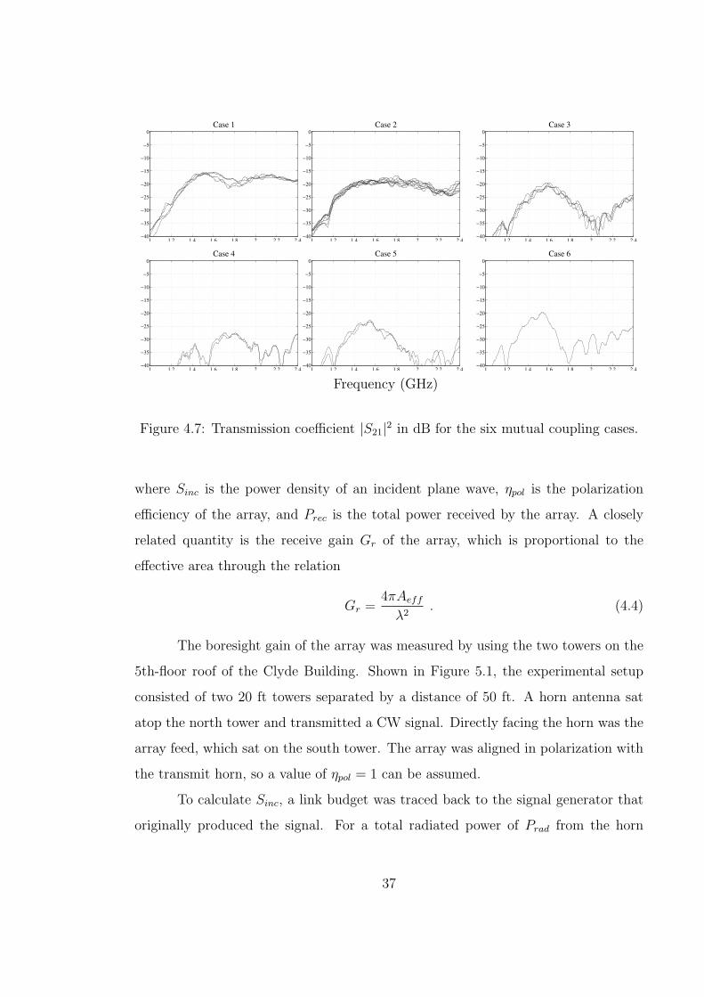
Mutual coupling between dipole elements has the potential to adversely affect

array performance [25]. It was quantified by treating the array as a 7-port microwave

network and then measuring the transmission coefficients with a network analyzer.

The results for this measurement are shown in Figure 4.7. Note that for each mea-

surement between two elements, the other five were terminated with open-circuit

loads.

From the geometry of the array, there are six unique arrangements between

any pair of elements [m,n]. Each of these arrangements can be described by the

horizontal and vertical offsets (x, y) between dipoles. Note that certain arrangements

have repeated symmetry between several elements. For example, we can expect the

mutual coupling between elements [1,2] to closely resemble that between elements

[5,1], since they both share the same offset of (0.6d, 0). The length d is defined

as 18.75 cm, which is one unit of wavelength at 1600 MHz. A summary of the

arrangements is provided below:

1. (x, y) = (0.6d, 0), shared by elements [2,1], [5,1], [4,3], and [7,6].

2. (x, y) = (0.3d,√

0.27d), shared by elements [3,1], [4,1], [6,1], [7,1], [3,2], [7,2],

[5,4], and [6,5].

3. (x, y) = (0.9d,√

0.27d), shared by elements [4,2], [6,2], [5,3], and [7,5].

4. (x, y) = (0.6d, 2√

0.27d), shared by elements [6,3], and [7,4].

5. (x, y) = (0, 2√

0.27d), shared by elements [7,3] and [6,4].

6. (x, y) = (1.2d, 0), shared by elements [5,2].

4.4 Gain and Effective Area

Recall from Section 2.5 that effective area is defined as

Aeff =Prec

ηpolSinc

(4.3)

36

1 1.2 1.4 1.6 1.8 2 2.2 2.4−40

−35

−30

−25

−20

−15

−10

−5

0Case 1

1 1.2 1.4 1.6 1.8 2 2.2 2.4−40

−35

−30

−25

−20

−15

−10

−5

0Case 2

1 1.2 1.4 1.6 1.8 2 2.2 2.4−40

−35

−30

−25

−20

−15

−10

−5

0Case 3

1 1.2 1.4 1.6 1.8 2 2.2 2.4−40

−35

−30

−25

−20

−15

−10

−5

0Case 4

1 1.2 1.4 1.6 1.8 2 2.2 2.4−40

−35

−30

−25

−20

−15

−10

−5

0Case 5

1 1.2 1.4 1.6 1.8 2 2.2 2.4−40

−35

−30

−25

−20

−15

−10

−5

0Case 6

Frequency (GHz)

Figure 4.7: Transmission coefficient |S21|2 in dB for the six mutual coupling cases.

where Sinc is the power density of an incident plane wave, ηpol is the polarization

efficiency of the array, and Prec is the total power received by the array. A closely

related quantity is the receive gain Gr of the array, which is proportional to the

effective area through the relation

Gr =4πAeff

λ2. (4.4)

The boresight gain of the array was measured by using the two towers on the

5th-floor roof of the Clyde Building. Shown in Figure 5.1, the experimental setup

consisted of two 20 ft towers separated by a distance of 50 ft. A horn antenna sat

atop the north tower and transmitted a CW signal. Directly facing the horn was the

array feed, which sat on the south tower. The array was aligned in polarization with

the transmit horn, so a value of ηpol = 1 can be assumed.

To calculate Sinc, a link budget was traced back to the signal generator that

originally produced the signal. For a total radiated power of Prad from the horn

37

Figure 4.8: Experimental setup on the roof of the Clyde building used to measurethe boresight gain of the 7-element array.

antenna, the power density incident on the array is given by

Sinc =GtPrad

4πr2(4.5)

where r = 50 ft is the distance between the towers and Gt is the gain of the transmit-

ting antenna. The antenna used as a transmitter was a Scientific Atlanta standard

gain horn model 12-1.7, which has a gain of 14.0 dBi at 1600 MHz. To calculate Prad,

it was necessary to account for the line loss from the signal generator to the horn

antenna, which was measured to be 5.4 dB at 1600 MHz. Also, one must account

for the impedance mismatch between the horn antenna and the transmission line.

Measured on a network analyzer, this introduced another 0.7 dB of loss. Thus, for a

total generated power of -85 dBm, Prad is found to be −91 dBm and Sinc is calculated

at 6.6× 10−15 W/m2.

The beamformer used to combine the array elements was an adaptive version

of LCMV,

w = R−1xxds (4.6)

38

where the array weight vector w was recalculated for every 2.5 ms of data and the

signal steering vector ds was calculated from training data. The total power received

by the array was then calculated using Equation 2.43, rewritten here as

Prec =1

α1α2

wHRssw (4.7)

where the constant α1 is given as

α1 =|gr|2|Z0|2

Rrad

(4.8)

and α2 is given as

α2 = wHAw . (4.9)

From the results in Section 4.2.1, the self-impedance Rrad of each antenna

element is approximately 50 Ω, as well as the characteristic impedance Z0. The gain

gr of each receiver channel was calibrated by feeding a known, −110 dBm signal to

each input and observing the total power at the each output1. The pattern overlap

matrix A, however, is difficult to measure in practice. Fortunately, A is a diagonally

dominant matrix whose main diagonal is identically all 1’s. This means the identity

matrix I is a close approximation to A, and has been observed to introduce an

uncertainty on the order of 0.5 dB or less. A close approximation to α2 is therefore

given by setting A = I, resulting in

α2 ≈ wHw . (4.10)

Using these values, the final power output power seen by the antenna array

was calculated at −124 dBm. This gives a total boresight gain of 13 dBi and an

effective area of 550 cm2. A good theoretical comparison is the Hertzian dipole

model from Section 2.1.2. Applying this model results in a total boresight gain of 12

dBi, which compares fairly well to the measured value.

1 Note that because the gain of each receiver channel is slightly different, Equation 4.8 had to beslightly modified so that gr is a vector that acts on each channel individually, rather than a singlescalar that acts on every channel at once.

39

40

Chapter 5

Antenna Test Range Receiver Design for the NRAO Head-

quarters

At the headquarters for the National Radio Astronomy Observatory (NRAO)

in Green Bank, West Virginia, there resides a twin-tower antenna test range. Cur-

rently, the test range is capable of producing accurate cut patterns for single element

antennas, but there is a desire to upgrade the range with the capability to measure

cut patterns for entire antenna arrays. This chapter presents the details of a receiver

design that is intended to replace the current system in use. To prove the design,

the seven-element prototype array was used as a test platform to demonstrate the

measurement of several cut patterns of array directivity.

Note that at the time of this writing, the design had not been finalized with

specific devices, but a demonstration had been performed with a prototype receiver

constructed out of spare parts. In the future, it will be important to catalog the final

devices and perform a robust characterization. There is also a great deal of work to

be done with the automation of the platform and post-processing of the data.

5.1 Geometry

The basic geometry of the range, shown in Figure 5.1, consists of two 35 ft

towers that are separated by a distance of 48 ft. The transmitter tower holds a horn

antenna (Tx) that beams energy across the range to the antenna under test (AUT).

On top of the receiver tower lies a turret which spins the AUT in azimuth. As the

turret spins, the electric field at the AUT is sampled over a specified range of angles,

providing a cut measurement of antenna gain.

41

Figure 5.1: Geometry for the antenna test range. The AUT sits on top of a rotatingturret, which allows the measurement of antenna gain.

The controls for the antenna range lie inside a small shack adjacent to the

receive tower, with long lines of coaxial cable connecting to the Tx and the AUT. In

order to measure a voltage phasor from the AUT, a receiver is required to translate

the high frequency signals down to baseband. Although a functional receiver is

already in use, the current system is relatively outdated and can only measure gain

for a single antenna. During the summer of 2005, the receiver was redesigned as part

of an upgrade to allow automated gain measurements of antenna arrays.

5.2 The Lock-In Amplifier

The most important device in the receiver is the lock-in amplifier (LIA). At

its core, the LIA is basically just a device that can take very precise measurements

of amplitude and phase on continuous wave (CW) signal. The specific device used in

the NRAO receiver is the Stanford Research Systems model SR830. A full product

description can be found online1, but the most important aspects will be provided in

this chapter.

1 http://www.srsys.com/products/SR810830.htm

42

Figure 5.2: Concept design for the single-stage lock-in receiver.

The LIA has two input channels, labeled reference (REF) and signal (SIG).

The REF input is a pure CW signal that tells the LIA which frequency to “lock in”

to. Once locked in, the LIA reads the SIG input and singles out any signal at the

same frequency as the reference. It then returns a complex number that represents

the phaser of the signal of interest (SOI). Because the LIA can single out a very

narrow bandwidth, it is capable of detecting extremely weak signals with a very high

precision.

In order to “lock in” to the REF signal, the LIA requires a stable sinusoid

with a minimum strength of 400mVpk−pk. The input impedance to the REF channel

is 1.0 MΩ, and the usable frequency range for measuring signals is 1.0mHz - 102kHz.

43

5.3 Theoretical Design Layout

Shown in Figure 5.2, the basic concept behind the antenna range receiver is

a dual, single-stage frequency translator. The system begins with a signal generator

that produces a CW signal at frequency fs which is then separated into two distinct

signals by a power splitter. One of these signals is mixed directly down to baseband

where it is sent to the REF channel of the LIA and serves as the reference. The

second signal is transmitted across the antenna range where it is received by the

AUT and then also mixed down to baseband. After mixing, the signal is fed to

the SIG channel of the lock-in amplifier, where it is measured as a voltage phasor

(x + jy). As the turret rotates, the phasor will vary in response to the directivity

of the AUT. To switch between antenna elements, a manifold of digitally controlled

switches (MUX) rests between the antenna array and the receiver.

5.4 LO Frequency

The final frequency at baseband is somewhat arbitrary, limited only by the

precision of the signal generators and the bandwidth of the LIA. In practice however,

it is sensible to keep the local oscillator frequency fLO as far from fs as possible. It

is therefore preferable to set the baseband frequency toward the maximum limit of

the LIA,

|fLO − fs| = 100 kHz . (5.1)

Since the signal frequency fs is a variable that changes with the specifications of the

AUT, fLO can be expressed as a function of fs,

fLO = fs ± 100 kHz . (5.2)

Note that it matters very little which LO frequency is chosen, since the baseband

frequency will be the same in either the plus or minus case.

5.5 Power Losses

The diagram in Figure 5.2 is merely a concept design and does not take into

account the non-ideal nature of the parts in a real system. In order to understand

44

Figure 5.3: Revised diagram indicating the major power losses.

the required changes for a practical receiver, it was helpful to first analyze the power

losses. The diagram in figure 5.3 presents a model of the major power losses in the

system. Under this model, there are four significant sources of power loss: Line

loss (Lline), space-propagation loss (Lspace), mixer conversion loss (Lmix), and power-

splitter loss (−3 dB).

5.5.1 Line Loss

The line losses in the system are a function of the transmission lines used to

carry signals. The system currently uses RG-213 coaxial cable, which is rated at 1600

MHz for a loss of 10 dB per 100 feet of cable. Using the geometry of the antenna

towers, the line losses are calculated as Lline1 = −8.3 dB and Lline2 = −3.5 dB. To

be conservative, these values should be rounded to −10 dB and −5 dB, respectively.

45

5.5.2 Propagation Loss

The free-space propagation loss is given by the Friis equation,

Lspace = GtGr

(λ

4πr

)2

(5.3)

where Gr is the AUT gain, Gt is Tx gain, and r = 48 ft is the distance between the

towers, and λ = 0.1875 m is the operational wavelength for the array feed. The value

of Gt can vary depending on the type of antenna used, but in practice it is common

to employ a horn antenna on the order of Gt = 10 dB (the actual value will vary

with frequency). Note that Gr has no distinct value, since it is a variable that will

change with AUT rotation. It is therefore useful to fix Gr = 1 and instead consider

it in terms of the dynamic range of the receiver. Using these values, the propagation

loss is on the order of Lspace ≈ −50 dB.

5.5.3 Conversion Loss

Conversion loss is encountered whenever a signal is translated in frequency by

a mixer. For a typical commercial mixer, the conversion loss is on the order of 7 dB.

5.5.4 Splitter Loss

The power splitter losses are simply the result of dividing a signal from one

transmission line into two, thus cutting the total power in half. For a standard

Wilkinson power divider, the loss from power splitting is fixed at −3 dB, plus a

negligible amount of insertion loss.

5.5.5 Power Budget

The maximum transmit power available from most signal generators is about

+10 dBm. Using the estimated loss values, it is a simple matter to calculate the

signal and reference powers to be on the order of

PSIG ≈ −65 dBm and

PREF ≈ −3 dBm .

46

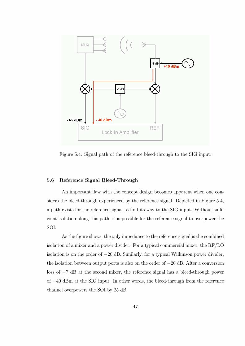
Figure 5.4: Signal path of the reference bleed-through to the SIG input.

5.6 Reference Signal Bleed-Through

An important flaw with the concept design becomes apparent when one con-

siders the bleed-through experienced by the reference signal. Depicted in Figure 5.4,

a path exists for the reference signal to find its way to the SIG input. Without suffi-

cient isolation along this path, it is possible for the reference signal to overpower the

SOI.

As the figure shows, the only impedance to the reference signal is the combined

isolation of a mixer and a power divider. For a typical commercial mixer, the RF/LO

isolation is on the order of −20 dB. Similarly, for a typical Wilkinson power divider,

the isolation between output ports is also on the order of −20 dB. After a conversion

loss of −7 dB at the second mixer, the reference signal has a bleed-through power

of −40 dBm at the SIG input. In other words, the bleed-through from the reference

channel overpowers the SOI by 25 dB.

47

Figure 5.5: An isolator made from an amplifier-attenuator pair.

5.7 Bleed-Through Solution

The solution to this problem is an increase in SOI power and an increase in

REF isolation. A simple way to increase the SOI power is to insert an amplifier after

the AUT, therefore boosting the SOI by +20 dB or more. To increase the isolation

from the REF signal, it is useful to employ the amplifier-attenuator pair shown in

Figure 5.5. For a signal traveling in the forward direction (port 1 to port 2), the

amplifier offsets the attenuator and nothing changes. For a signal traveling in the

reverse direction, the directivity of the amplifier combines with the attenuator to

drastically reduce the signal power. Thus, to a good approximation, the S-parameter

matrix can be modeled as

S =

0 1

D+L

GL

1

(5.4)

where D is the amplifier directivity, G is the amplifier gain, and L is the attenuator

loss.

A good, high-isolation amplifier will have a directivity of at least D = 30 dB

and should have a gain of at least of G = 20 dB. To offset the gain of the amplifier,

the attenuator should then have a loss of L = 20 dB as well. The amplifier-attenuator

pair therefore gives an extra 50 dB of isolation between mixer 1 and mixer 2. The

final result is a power of −45 dBm from the SOI and a power of −93 dBm from

the REF bleed-through. This implies a lower bound of Gr = −45 dBi before the

48

bleed-through from the reference signal is on the same order of magnitude as the

SOI. In practice, however, it would be rare to expect any precision below −30 dBi.

5.8 Reference Input Power

Recall from Section 5.2 that the REF input to the LIA requires a signal

strength of 400 mVpk−pk on a 1.0 MΩ impedance. For a characteristic impedance of

50 Ω from the input line, this requires the REF input to have a minimum power level

of −4 dBm. When compared to the calculated value of −3 dBm, the LIA is only

marginally capable of locking in to the reference signal. To address this concern, an

amplifier should be added at the REF input to the LIA with a gain of about +10

dB.

5.9 Low-Pass Filters

The final modification to the design requires two low-pass filters at the inputs.

Because of harmonic distortion, upper-sideband mixing, and RF bleed-through, there

exists the potential for high-frequency signals to make their way to the LIA inputs. To

alleviate this concern, it is prudent to insert a low-pass filter with a cutoff frequency

of 100 kHz at each input to the LIA.

5.10 Summary

The final receiver design is shown in Figure 5.6. Note that the design is

basically the same as that in Figure 5.2, but with a few minor modifications to

account for the non-ideal nature of the system. Particularly, the additions include

an amplifier-attenuator pair to help isolate mixer 1 from mixer 2, two amplifiers to

boost the SIG and REF powers, and two low-pass filters to remove the undesirable

high-frequency content.

Currently, the receiver has no specified part numbers, since all of the testing

was performed with devices that were literally scrounged out of boxes of spare parts.

The current design has, however, been demonstrated on the prototype array feed,

with excellent results. The final task, therefore, is to find commercial devices with

49

Figure 5.6: Final design for the NRAO test-range receiver.

which to construct a permanent receiver. Once this task has been completed, all

future work with the range upgrade can be shifted to the user interface and data

acquisition.

5.11 Array Directivity Measurements

In July, 2005, directivity measurements were performed on the array feed

while using the prototype receiver design in Figure 5.6. An example of the experi-

mental setup is depicted in Figure 5.7, which shows the array feed atop the rotating

turret along the co-polarized, H-plane cut. For cut measurement, the phase center of

rotation was fixed at the ground plane beneath the center element. For each phasor

measurement, the load impedances at the other antenna elements were open-circuits.

50

Figure 5.7: The seven-element array at the NRAO test range in Green Bank, WV.The incident electric field is co-polarized with the array elements and the rotation isalong the H-plane.

5.11.1 Calibration

From the geometry of the array, it is clear to see that the array elements are

all coplanar when viewed from boresight. It is therefore reasonable to assume that

an incident plane-wave from boresight should result in roughly identical excitations

in every element. Using this assumption, it was possible to account for the relative

variations in gain and phase delay between each channel. Note, however, that this

information is only sufficient to produce a relative measurement of directivity. An

absolute measurement was obtained in Section 4.4, which placed the boresight gain

at 13 dBi.

51

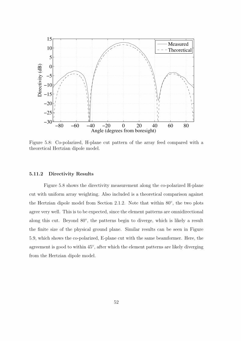
−80 −60 −40 −20 0 20 40 60 80−30

−25

−20

−15

−10

−5

0

5

10

15

Angle (degrees from boresight)

Dire

ctiv

ity (d

B)

MeasuredTheoretical

Figure 5.8: Co-polarized, H-plane cut pattern of the array feed compared with atheoretical Hertzian dipole model.

5.11.2 Directivity Results

Figure 5.8 shows the directivity measurement along the co-polarized H-plane

cut with uniform array weighting. Also included is a theoretical comparison against

the Hertzian dipole model from Section 2.1.2. Note that within 80, the two plots

agree very well. This is to be expected, since the element patterns are omnidirectional

along this cut. Beyond 80, the patterns begin to diverge, which is likely a result

the finite size of the physical ground plane. Similar results can be seen in Figure

5.9, which shows the co-polarized, E-plane cut with the same beamformer. Here, the

agreement is good to within 45, after which the element patterns are likely diverging

from the Hertzian dipole model.

52

−80 −60 −40 −20 0 20 40 60 80−30

−25

−20

−15

−10

−5

0

5

10

15

Angle (degrees from boresight)

Dire

ctiv

ity (d

B)

MeasuredTheoretical

Figure 5.9: Co-polarized, E-plane cut pattern of the array feed compared with atheoretical Hertzian dipole model.

53

54

Chapter 6

RFI Mitigation with the Focal-Plane Array

This chapter describes the characterization of the focal plane array in con-

junction with a three-meter parabolic reflector. It includes a description of the

experimental setup, a boresight gain measurement, and the results of several RFI

scenarios.

6.1 Experimental Setup

To simulate an astronomical observation in the presence of an interferer, the

experiment required two transmitters and a receiver. One of the transmitters acted

as a signal of interest (SOI) at boresight, while the other acted as an interferer in the

deep sidelobes. To obtain a clear line of sight between the antennas, they were all

positioned on separate rooftops among BYU campus. Figure 6.1 shows an overhead

perspective of the antenna positions.

The receive antenna consisted of the prototype array feed mounted at the focal

plane of a three-meter parabolic dish (Figure 6.2). Antenna 1 of the VSA was chosen

for this role because it has a clear line of sight to the rooftops of BYU campus. The

SOI was a standard gain horn positioned at boresight to the receiver. The roof of the

Kimball Tower was a convenient place for this antenna, due to its easy access, large

height, electrical outlets, and safety fencing. The interferer used a half-wave dipole

antenna that rested on the observation deck of the Joseph F. Smith Building, which

also has electrical access and safety fencing. In particular, when viewed the from the

Clyde Building, the observation deck spans a 4 arc from 27 − 31 relative to the

SOI. This makes it ideal for testing array performance with a moving interferer.

55

Figure 6.1: Rooftop positions of the antennas. The array feed and reflector arelocated on the roof of the Clyde Building. The horn antenna (signal) is positionedat boresight to the reflector and is located on the Kimball Tower. The interferer is asmall dipole located on the observation deck of the Joseph F. Smith Building. Imagetaken from www.maps.google.com.

56

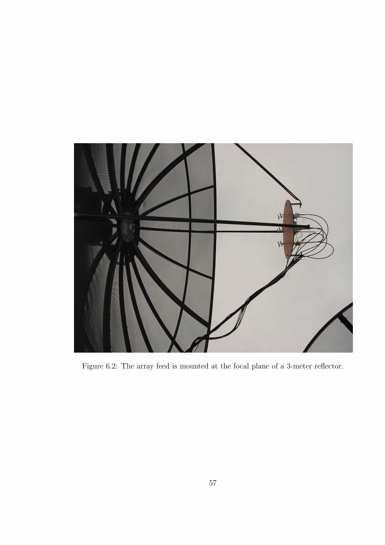
Figure 6.2: The array feed is mounted at the focal plane of a 3-meter reflector.

57

6.2 Calibration and Alignment

Before installing the array onto the reflector, the gain of each receiver channel

was measured by feeding a continuous wave (CW), -110 dBm signal into each chan-

nel. The individual gains were then calculated by measuring the total power at the

output and comparing with the known value at the input. This information provides

meaningful units of voltage and power as seen by the individual antenna elements,

which is necessary when calculating the effective area of the receiver or when using

the array as a radiometer.

After calibration, the array was installed onto the support struts of Antenna 1.

In order to accept the array feed, the support struts had to be modified by bending

them outwards into a position that will fit with the array stand-offs. The center

element of the array was located at the focal point of the dish, and the ground plane

was parallel with the directrix plane of the reflector.

The final step was an alignment of the reflector so that it pointed directly at

the SOI. This was accomplished by first activating the transmitter and broadcasting a

strong, CW signal. The reflector was then scanned in azimuth and elevation until the

power observed at the center element was maximized. The transmitter was similarly

aligned by scanning the horn antenna in azimuth, elevation, and polarization until

the observed power was maximized at the center element.

6.3 Training Data

Training data was obtained by sampling under controlled conditions. For

example, the noise correlation matrix Rnn was obtained by sampling while the SOI

and the interferer were both deactivated. The signal correlation matrix Rss was

obtained by sampling while the SOI was active with a very high SNR. Similarly,

the interferer correlation matrix Rii was obtained by sampling while the interferer

was active with a very high INR. The steering vectors ds and di were obtained by

computing the principle eigenvectors of their respective correlation matrices.

58

6.4 Effective Area and Aperture Efficiency

The effective area of the array feed was measured by using the same link-

budget procedure as that in Section 4.4. After a simple modification of the Friis

equation, the effective area of the center element in the array is given as

Aeff =4πr2Prec

GtPrad

(6.1)

where r is the distance between the source and receive antennas, Prec is the total

received power at the center element, Gt is the gain of the transmit antenna, and

Prad is the total radiated power. The distance r was measured with a rangefinder

and found to be 256 m. The transmit antenna was the same standard gain horn used

in Section 4.4, which has a value of Gt = 14 dBi at 1600 MHz. The transmission

from the signal generator was a CW waveform at -60 dBm, but the measured line

losses and impedance mismatches subtracted 3 dB. Thus, the total radiated power

was Prad = -63 dBm.

The highest value for Prec was obtained by using an adaptive LCMV beam-

former given by

w = R−1xx ds . (6.2)

The array weight vector w was recalculated for every 4.9 ms segment of data1 and

the principle eigenvector of Rxx was used for ds. The total output power was then

calculated using Equation 2.43,

Prec =1

α1α2

wHRssw

where α1 and α2 were calculated using the methods outlined in Section 4.4. The

result was a total received power of −101.6 dBm, which yields an effective area of

4.56 m2. For a physical reflector area Aphy, the aperture efficiency ηap is defined as

ηap =Aeff

Aphy

. (6.3)

For a diameter of 3.0 meters at rim of the reflector, the physical collecting area is

7.07 m2, and the aperture efficiency is found to be 0.64. This compares well with the

1 4.9 ms represents a single block of unpacked data, and therefore made a convenient choicefrom a programming perspective.

59

aperture efficiencies of standard reflector antennas. For example, a reflector antenna

that is optimized for gain can reach an aperture efficiency as high as 0.80. Often

times, however, gain will be traded off for lower spillover efficiency, and typically

results in an aperture efficiency as low as 0.55.

It is important to note that because of antenna misalignments, multipath, loss

uncertainties, and gain variations, the confidence for these measurements is on the

order of ±1.0 dB in the signal path. The only way to reliably reduce this uncertainty

would be to repeat the entire measurement inside an anechoic chamber, which is

impractical. Converting this uncertainty into the effective area gives a lower bound

at 3.62 m2 (ρ = 0.51), and an upper bound of 5.74 m2 (ρ = 0.81).

6.5 Stationary Interferer

The first interference scenario was a weak SOI in the presence of a powerful

interferer. The SOI was a CW transmission at 1611.3 MHz with an output power of

−110 dBm. This value was chosen because it placed the SOI below the non-integrated

noise floor of the receiver. The interferer was a 0 dBm FM transmission centered

at 1611.3 MHz, with 30 kHz of deviation and 1.0 kHz of modulation. This scenario

represents a typical encounter in radio astronomy where a weak SOI is overpowered

by an off-boresight interferer at the same frequency.

6.5.1 Single Element

Figure 6.3 shows the non-integrated power spectral density (PSD) of the signal

as seen by the center element of the array. To reduce spectral leakage, the data has

been windowed by a Hanning function. Also, to flatten out the noise floor, a baseline

subtraction was performed by dividing out the PSD of a noise-only data set. This

graph represents the control signal that would be seen by a standard, single-feed

receiver in a radio telescope. Because the SOI is so weak, the only way to distinguish

it from the noise floor is through integration.

Figure 6.4 shows the resulting PSD after 10 seconds of integration. As ex-

pected, the noise floor is smoothed out, but the FM interferer remains and the SOI is

60

not resolved. If this were an actual scientific observation, the data would be useless

and the observation would have to be discarded.

6.5.2 Max SINR using Interferer Subspace Partitioning

Because the interferer was so much more powerful than the noise floor or the

SOI, it was possible to solve for the max-SINR beamformer through a process called

interferer subspace partitioning (ISP). ISP works by using the principle eigenvector

of Rxx as an estimate for di2. The interferer correlation matrix Rii is then estimated

by using

Rii = didHi . (6.4)

The interference-plus-noise correlation matrix RNN is estimated by using RNN =

Rii + Rnn, where Rnn is obtained from training data. Finally, the array weight

vector w is given by the principle eigenvector to the generalized eigenvalue problem,

Rssw = (SINR)RNNw (6.5)

which is simply the max-SINR beamformer. Figure 6.5 shows the results from this

method using an update rate of 4.9 ms. As can be seen, the FM interferer is almost

completely removed and the SOI is recovered.

6.6 Non-stationary Interferer

A more typical encounter in radio astronomy is a non-stationary interferer,

such as radar bounce from an aircraft, satellite broadcasts, or the relative motion of

the telescope while tracking an object in the sky. This situation was simulated by

carrying the interfering antenna along the observation deck of the Joseph F. Smith

Building and walking at a normal pace. As seen from the receiver at the Clyde

Building, the angular velocity was on the order of 0.1/s, which is typical for a

satellite in medium Earth orbit. During this trial, the SOI was a CW transmission

at −90 dBm with a −10 dBm FM interferer overlapping in frequency.

2 See section 2.2.1

61

1610.9 1611 1611.1 1611.2 1611.3 1611.420

25

30

35

40

45

50

55

60

Frequency (MHz)

PSD

(Arb

dB/H

z)

Figure 6.3: Non-integrated PSD as seen by the center element alone. A CW signalis buried beneath the noise floor with an FM interferer overlapping. Due to baselinesubtraction, the units for power are arbitrary.

1610.9 1611 1611.1 1611.2 1611.3 1611.420

25

30

35

40

45

50

55

60

Frequency (MHz)

PSD

(Arb

dB/H

z)

Figure 6.4: PSD of the center element after 10 seconds of integration. The noise flooris smoothed out, but the FM interferer remains and completely masks the signal ofinterest.

62

1610.9 1611 1611.1 1611.2 1611.3 1611.420

25

30

35

40

45

50

55

60

Frequency (MHz)

PSD

(Arb

dB/

Hz) SIGNAL

Figure 6.5: PSD of the Max-SINR beamformer using interferer subspace partitioningon the stationary interferer. The total integration time is 10 seconds. Note how theinterferer is almost completely removed and the signal is recovered.

6.6.1 Single Element

Figure 6.6 shows the PSD as seen by the center element with 10 seconds of

integration on the non-stationary interferer. As expected, the interferer dominates

the signal and the SOI is not apparent.

6.6.2 Max SINR using Interferer Subspace Partitioning

Figure 6.7 shows the max-SINR beamformer from Section 6.5.2 with an update

every 4.9 ms. Even though it was non-stationary, the interferer has been mitigated

and the SOI is recovered.

63

1610.9 1611 1611.1 1611.2 1611.3 1611.420

25

30

35

40

45

50

55

60

Frequency (MHz)

PSD

(Arb

dB/H

z)

Figure 6.6: PSD as seen by the center element after 10 seconds of integration. Theinterferer is traveling at a velocity of approximately 0.1/s.

1610.9 1611 1611.1 1611.2 1611.3 1611.420

25

30

35

40

45

50

55

60

Frequency (MHz)

PSD

(Arb

dB/H

z) SIGNAL

Figure 6.7: PSD of the Max-SINR beamformer using interferer subspace partitioningon the moving interferer. The total integration time is 10 seconds. Again, theinterferer is almost completely removed and the signal is recovered.

64

0 5 10 15 20 25 30 35 40−5

0

5

10

15

20

25

30

35

40

Center Element INR (dB)

IRR

(dB)

SINR−ISPSINR−TRNLCMVGAIN

Figure 6.8: Interference rejection ratio of the beamformers as a function of inter-ference to noise ratio at the center element. The red line represents y = x, whichindicates the interferer is either at or below the noise floor.

6.7 Performance Versus Interferer Power

The performance of a given beamformer depends greatly on the relative power

levels between the signal and the interferer. To measure this effect, several measure-

ments were taken with a varying amount of input power from the interferer. A useful

metric for beamformer performance is the interference rejection ratio (IRR), which

is defined as the INR seen by the center element (INRel1) divided by the INR as seen

by the beamformer of interest (INRx), and written as

IRR =INRel1

INRx

. (6.6)

Figure 6.8 summarizes the performance of several beamformer techniques as

a function of interferer power level. The first beamformer (SINR-ISP) represents

65

max-SINR using interferer subspace partitioning with an update every 4.9 ms. The

second beamformer (SINR-TRN) represents a single max-SINR beamformer calcu-

lated once from training data. The third beamformer (LCMV) represents the LCMV

beamformer with an update every 4.9 ms. The fourth beamformer (GAIN) is a single

max-gain beamformer calculated from training data, and represents a control signal

without any interference mitigation at all.

It is interesting to note how there is no ideal beamformer for the entire range

of interferer power. At low power levels (< 10 dB), the best results were obtained by

using the SINR-TRN beamformer, which seems to provide a relatively fixed amount

of interference rejection on the order of 18 dB. At medium power levels (10 - 25 dB),

the best results were obtained from the SINR-ISP beamformer, with LCMV following

closely. At high power levels (> 25 dB), LCMV and SINR-ISP begin to wane, but

with LCMV performing better. As expected, the max-gain beamformer provided no

interference rejection, but rather increased the power in the interferer, as indicated

by the negative IRR.

6.8 Correlation Time and Non-Stationarity

When calculating a correlation matrix, it is generally preferable to average for

as long as possible in order to reduce estimation error caused by noise. A moving

interferer, however, has non-stationary statistics. This places an upper limit to the

length of a correlation window before non-stationarity influences an estimate. Thus,

there is an inherent trade-off in the estimation error. If the correlation window is too

short, then estimation error is dominated by noise. If the correlation window is too

long, then estimation error is dominated by non-stationarity.

Figure 6.9 shows the IRR of two beamformers as a function of correlation

time, where the data set is the stationary interferer. As expected, the IRR is low

over short correlation windows because the correlation estimate is dominated by

noise. However, there is also an upper limit to the benefits of averaging a correlation

matrix. After 5 ms or so, the IRR levels off and shows no improvement over longer

averaging windows.

66

10−5 10−4 10−3 10−2 10−1 10012

14

16

18

20

22

24

26

28

Correlation Window (s)

IRR

(dB

)

SINR−ISPLCMV

Figure 6.9: Interference rejection ratio as a function of correlation length for thestationary interferer.

It is interesting to note how subspace partitioning results in much greater

interference mitigation than LCMV. It is also interesting to note how long-term

correlation does not perfectly mitigate the interferer. This is likely the result of

small-scale non-stationarity in the interferer correlation matrix. Minor perturbations

due to mechanical vibration and multipath can cause the instantaneous correlation

matrix to deviate slightly from its mean value. The interference rejection is therefore

very high, but can not perfectly track the instantaneous changes.

67

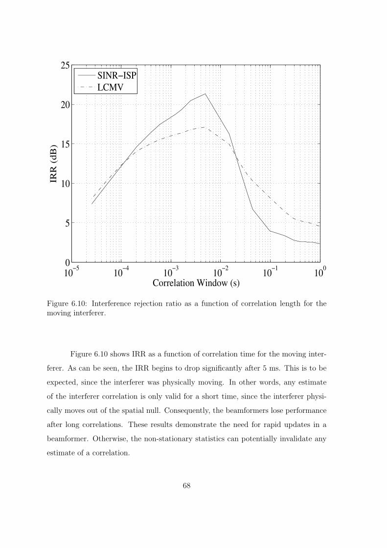
10−5 10−4 10−3 10−2 10−1 1000

5

10

15

20

25

Correlation Window (s)

IRR

(dB

)

SINR−ISPLCMV

Figure 6.10: Interference rejection ratio as a function of correlation length for themoving interferer.

Figure 6.10 shows IRR as a function of correlation time for the moving inter-

ferer. As can be seen, the IRR begins to drop significantly after 5 ms. This is to be

expected, since the interferer was physically moving. In other words, any estimate

of the interferer correlation is only valid for a short time, since the interferer physi-

cally moves out of the spatial null. Consequently, the beamformers lose performance

after long correlations. These results demonstrate the need for rapid updates in a

beamformer. Otherwise, the non-stationary statistics can potentially invalidate any

estimate of a correlation.

68

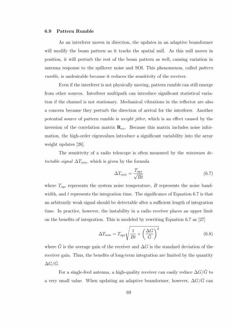
6.9 Pattern Rumble

As an interferer moves in direction, the updates in an adaptive beamformer

will modify the beam pattern as it tracks the spatial null. As this null moves in

position, it will perturb the rest of the beam pattern as well, causing variation in

antenna response to the spillover noise and SOI. This phenomenon, called pattern

rumble, is undesirable because it reduces the sensitivity of the receiver.

Even if the interferer is not physically moving, pattern rumble can still emerge

from other sources. Interferer multipath can introduce significant statistical varia-

tion if the channel is not stationary. Mechanical vibrations in the reflector are also

a concern because they perturb the direction of arrival for the interferer. Another

potential source of pattern rumble is weight jitter, which is an effect caused by the

inversion of the correlation matrix Rxx. Because this matrix includes noise infor-

mation, the high-order eigenvalues introduce a significant variability into the array

weight updates [26].

The sensitivity of a radio telescope is often measured by the minimum de-

tectable signal ∆Tmin, which is given by the formula

∆Tmin =Tsys√Bt

(6.7)

where Tsys represents the system noise temperature, B represents the noise band-

width, and t represents the integration time. The significance of Equation 6.7 is that

an arbitrarily weak signal should be detectable after a sufficient length of integration

time. In practice, however, the instability in a radio receiver places an upper limit

on the benefits of integration. This is modeled by rewriting Equation 6.7 as [27]

∆Tmin = Tsys

√1

Bt+

(∆G

G

)2

(6.8)

where G is the average gain of the receiver and ∆G is the standard deviation of the

receiver gain. Thus, the benefits of long-term integration are limited by the quantity

∆G/G.

For a single-feed antenna, a high-quality receiver can easily reduce ∆G/G to

a very small value. When updating an adaptive beamformer, however, ∆G/G can

69

increase by a great deal. The reason is because pattern rumble effectively changes

the beamformer response to the SOI and noise. As seen by the receiver, the result is

equivalent to an increase in ∆G.

To understand how pattern rumble affects the final sensitivity, consider the

turning point where pattern rumble overpowers the noise variance. This is the point

at which1

Bt=

(∆G

G

)2

. (6.9)

For perspective purposes, a standard bandwidth is chosen as B0 = 1.0 kHz. The

maximum integration time tmax is then defined as

tmax =1

B0

(∆GG

)2 . (6.10)

In other words, tmax represents the maximum integration time where the noise vari-

ance, at a bandwidth of B0, is stronger than receiver instability. Integration beyond

this time will still decrease ∆Tmin, but the marginal benefit approaches zero.

If the amplifier gain of each channel is assumed to be relatively constant, then

the quantity ∆G/G is dominated by pattern rumble. It can therefore be measured

as the time-variation in SNR from the adaptive beamformer. Note, however, that

pattern rumble is not the only phenomenon that can introduce jitter in the SNR.

For example, mechanical vibrations in the reflector will introduce jitter in the SOI

that is independent of the pattern rumble. It should also be noted that the measured

noise floor periodically rose and fell by roughly 1.0 dB. This was likely the result

of broadband interference that reflected off of the Kimball Tower and into the main

beam of the receiver.3

To normalize these effects, the array gain Ga was measured against the max-

gain beamformer (which uses non-updating weights) such that

G = Ga =SNRx

SNRgain

. (6.11)

3 Similar interference has been observed at the same frequencies reflecting off other buildings inthe area.

70

This expression effectively cancels out the effects of outside influences, since the vari-

ations in SNR will be roughly the same for both beamformers. Thus, the remaining

jitter should be due to pattern rumble from the adaptive beamformer.

Figure 6.11 shows the observed pattern rumble for three adaptive beamformers

acting on the fixed interferer. Each point represents a sliding window of one-second

integration before calculating Ga. The SINR-TRN beamformer represents a control

signal because it used fixed weights, while LCMV and SINR-ISP were updated every

4.9 ms. From the data, the maximum integration times were calculated as 1.7 seconds

for SINR-TRN, 1.7 seconds for LCMV, and 1.2 seconds for SINR-ISP. Thus, the

observed pattern rumble for the updated beamformers was on the same order of

magnitude as the fixed-weight beamformer. This result suggests that mitigation of a

stationary beamformer does not introduce any significant pattern rumble above the

natural rumble of the system.

Figure 6.12 shows the observed pattern rumbles for the case of the moving

interferer. In this case, the maximum integration time for the SINR-TRN beamformer

was slightly higher, measuring at a value of 3.3 seconds. The updated beamformers,

however, measured significantly lower, both reaching a maximum integration time

of only 0.3 seconds. This result shows how adaptively mitigating an interferer can

reduce the effective sensitivity of a radio telescope by as much as one-tenth. In the

future, it may be possible to construct a beamformer that minimizes this effect, but

further research will be required.

71

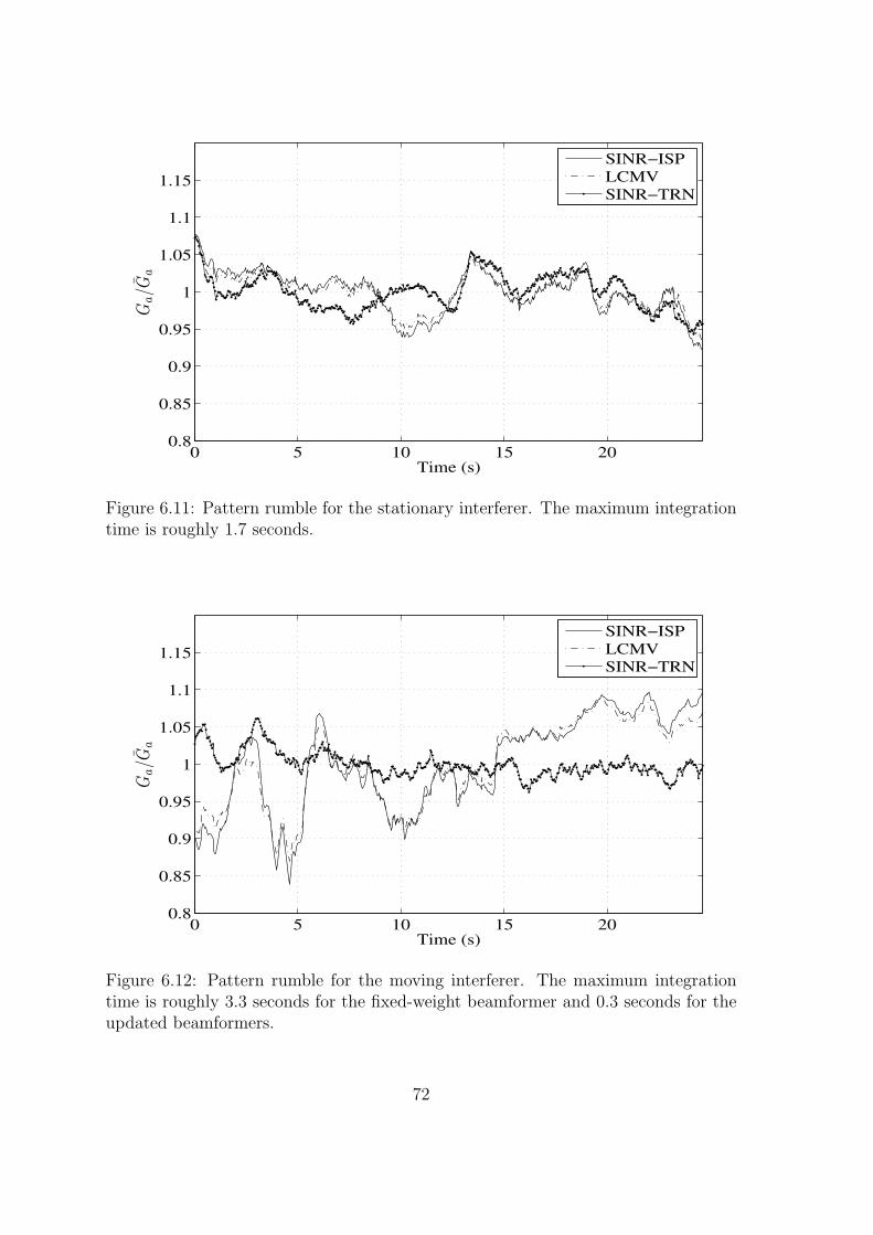
0 5 10 15 200.8

0.85

0.9

0.95

1

1.05

1.1

1.15

Time (s)

Ga/G

a

SINR−ISPLCMVSINR−TRN

Figure 6.11: Pattern rumble for the stationary interferer. The maximum integrationtime is roughly 1.7 seconds.

0 5 10 15 200.8

0.85

0.9

0.95

1

1.05

1.1

1.15

Time (s)

Ga/G

a

SINR−ISPLCMVSINR−TRN

Figure 6.12: Pattern rumble for the moving interferer. The maximum integrationtime is roughly 3.3 seconds for the fixed-weight beamformer and 0.3 seconds for theupdated beamformers.

72

Chapter 7

Conclusions and Future Work

The primary contribution of this thesis has been the design and construction

of a seven-element array feed with seven corresponding receiver channels. The array

was then demonstrated by mitigating a strong interferer to recover a weak signal of

interest. The results of that demonstration have proven useful in characterizing the

array feed, as well as in highlighting the major problems that need to be solved. The

following sections discuss several of the outstanding issues that will require future

research.

7.1 Robust Beamformers

Paradoxically, the stronger an interferer is, the more effectively it can be

mitigated. When the interfering signal is on the same order of power as the signal

of interest, however, it becomes far more difficult to mitigate. Little research has

been applied towards this issue, since it is not as important to communications or

radar applications as it is to radio astronomy. Many solutions have been suggested,

such as subspace-tracking and multiple null placement [26], but they have yet to be

demonstrated with an array feed.

7.2 Array Weight Normalization

In order to be useful as a radiometer, it is important to properly scale the

output of a beamformer. Otherwise, the array weights will artificially add power to

the final signal. Mathematically, this is accomplished by enforcing the criterion

wHAw = 1 (7.1)

73

where A is the pattern overlap matrix. The problem with this condition is that A

is rarely available, which means the final power as seen by the array is difficult to

precisely measure. Although the identity matrix makes for a reasonable approxi-

mation, the requirements of radio astronomy are too precise for it to be used with

astronomical signals.

7.3 Optimal Feed Placement

The placement of the array can have a significant impact on the performance

of the receiver. For the experiments in Chapter 6, the array feed was placed such

that the center element was at the focal point of the reflector. This placement was ad

hoc, however, because there was little research available that might suggest a more

ideal location. It is possible that the array would perform better if the focal point

were located at the ground plane below the center element, but the only way to be

sure would be to measure (or simulate) the array gain at varying locations.

7.4 Mutual Coupling

Mutual coupling has the potential to lower sensitivity, increase noise temper-

ature, and impair the performance of a beamformer. It is possible to alleviate this

problem through the use of matching networks, but this has yet to be extensively

studied or implemented with the array feed.

7.5 Sensitivity

Although the aperture efficiency of the array feed performed well, the most

important metric to radio astronomers is sensitivity. Measuring this will require a

measurement of spillover efficiency, as well as a deeper understanding about mutual

coupling and pattern rumble.

7.6 Array Expansion

Currently, there is work in progress to expand the number of array elements

from 7 to 19. With more array elements, it would be possible to mitigate more

74

independent interferers with less trade-off in sensitivity. Due to its physical size and

weight, however, it is unlikely that a 19-element array would be compatible with our

3 meter dishes. A larger reflector would experience less signal blockage and also be

capable of mechanically supporting the extra weight.

7.7 Astronomical Observation on the GBT

The ultimate goal for the array feed is to demonstrate its performance on the

Green Bank Telescope (GBT), and any design choices should be made with this goal

in mind. If a focal plane array were used to mitigate a real satellite interferer and

recover a legitimate astronomical signal, then it will have proven its usefulness to the

radio astronomy community.

75

76

Bibliography

[1] H. Rottgering, “LOFAR, a new low frequency radio telescope,” New Astronomy

Reviews, vol. 47, no. 2, pp. 405–409, September 2003. 2

[2] D. DeBoer, W. J. Welch, J. Dreher, J. Tarter, L. Blitz, M. Davis, M. Fleming,

D. Bock, G. Bower, J. Lugten, Girmay-Keleta, L. D’Addario, G. Harp, R. Ack-

ermann, S. Weinreb, G. Engargiola, D. Thornton, and N. Wadefalk, “The Allen

telescope array,” Proceedings of the SPIE, vol. 5489, pp. 1021–1028, 2004. 2

[3] P. J. Hall, The Square Kilometre Array: An Engineering Perspective, 1st ed.

Springer, 2005. 2

[4] J. R. Fisher, “Signal analysis and blanking experiments on DME interference,”

NRAO Electronics Division, Tech. Rep. 313, April 2004. 2

[5] S. Ellingson, J. Bunton, and J. Bell, “Removal of the GLONASS C/A signal

from OH spectral line observations using a parametric modeling technique,”

The Astrophysical Journal Supplement Series, no. 135, pp. 87–93, July 2001. 2

[6] B. Smolders and G. Hampson, “Deterministic RF nulling in phased arrays for

the next generation of radio telescopes,” IEEE Transactions on Antennas and

Propagation, vol. 44, no. 8, pp. 13–22, 2002. 2

[7] J. L. Campbell, “The development of a small scale radio astronomy image syn-

thesis array for research in radio frequency interference mitigation,” Master’s

thesis, Brigham Young University, 2005. 2

[8] A. J. Poulsen, “Real-time adaptive cancellation of satellite interference in radio

astronomy,” Master’s thesis, Brigham Young University, 2003. 2

77

[9] B. D. Jeffs, L. Li, and K. F. Warnick, “Auxiliary antenna-assisted interference

mitigation for radio astronomy arrays,” IEEE Transactions on Signal Processing,

vol. 53, no. 2, pp. 439–451, February 2005. 2

[10] C. K. Hansen, “Beamforming techniques and interference mitigation using a

multiple feed array for radio astronomy,” Master’s thesis, Brigham Young Uni-

versity, 2004. 2

[11] S. J. Blank and W. A. Imbraile, “Array feed synthesis for correction of reflec-

tor distortion and verneir beamsteering,” IEEE Transactions on Antennas and

Propagation, vol. 36, no. 10, pp. 1351–1358, October 1988. 2

[12] L. Staveley-Smith, W. E. Wilson, T. S. Bird, M. J. Disney, R. D. kers, K. C.

Freeman, R. F. Haynes, M. W. Sinclair, R. A. Vaile, R. L. Webster, and A. E.

Wright, “The Parkes 21-cm multibeam receiver,” Publications of the Astronom-

ical Society of Australia, vol. 13, pp. 243–248, 1996. 2

[13] B. S. Koribalski, “The H1 Parkes all-sky survey (HIPASS),” ASP Converence

Series, vol. 276, p. 72, October 2002. 2

[14] M. V. Ivashina, J. G. bij de Vaate, R. Braun, and J. Bregman, “Focal plane

arrays for large reflector antennas: First results of a demonstrator project,”

Proceedings of the SPIE, vol. 5489, pp. 1127–1138, September 2004. 2

[15] J. R. Fisher and R. F. Bradley, “Full-sampling array feeds for radio telescopes,”

Proceedings of the SPIE, vol. 4015, pp. 308–319, 2000. 2

[16] C. K. Hansen, K. F. Warnick, B. D. Jeffs, J. R. Fisher, and R. Bradley, “Inter-

ference mitigation using a focal plane array,” Radio Science, vol. 40, June 2005.

3, 13, 31

[17] B. T. Walkenhorst, “Development of a radio telescope receiver for research in

radio astronomy interference mitigation,” Master’s thesis, Brigham Young Uni-

versity, 2001. 3, 15

78

[18] J. Li and P. Stoica, Robust Adaptive Beamforming. John Wiley & Sons, Inc,

2006. 5

[19] J. A. Kong, Electromagnetic Wave Theory. EMW Publishing, 2000. 7

[20] T. K. Moon and W. C. Stirling, Mathematical Methods and Algorithms for Signal

Processing. Prentice Hall, 2000. 13

[21] K. F. Warnick and B. D. Jeffs, “Receive array gain and aperture efficiency,”

2006. 14

[22] D. M. Pozar, Microwave Engineering, 2nd ed. Wiley, 1998. 26

[23] J. R. Fisher and R. F. Bradley, “Full-sampling focal plane array,” Imaging at

Radio Through Submillimeter Wavelengths, vol. 217, pp. 11–18, December 1999.

31

[24] R. S. Elliott, Antenna Theory and Design. IEEE Press, 2003. 31

[25] K. F. Warnick and M. A. Jensen, “Effects of mutual coupling on interference

mitigation with a focal plane array,” IEEE Transactions on Antennas and Prop-

agation, vol. 53, no. 8, pp. 2490–2498, August 2005. 36

[26] G. A. Hampson and S. W. Ellingson, “A subspace-tracking approach to inter-

ference nulling for phased array-based radio telescopes,” IEEE Transactions on

Antennas and Propagation, vol. 50, no. 1, January 2002. 69, 73

[27] J. D. Kraus, Radio Astronomy, 2nd ed. Cygnus-Quasar Books, 1986. 69

79