Thesis Proposal :Switching Linear Dynamic Systems with

Higher-order Temporal Structure

Sang Min Ohsangmin@cc.gatech.edu

28th May 2008

Contents

1 Introduction 11.1 Automated Temporal Sequence Analysis . . . . . . . . . . . . . . . . . . . . . . . . . . . . . . . . . 11.2 Learning from examples . . . . . . . . . . . . . . . . . . . . . . . . . . . . . . . . . . . . . . . . . 31.3 Model-based Approach : SLDSs . . . . . . . . . . . . . . . . . . . . . . . . . . . . . . . . . . . . . 31.4 Beyond standard SLDSs . . . . . . . . . . . . . . . . . . . . . . . . . . . . . . . . . . . . . . . . . 4

1.4.1 Duration modeling for LDSs . . . . . . . . . . . . . . . . . . . . . . . . . . . . . . . . . . . 41.4.2 Explicit modeling of global parameters . . . . . . . . . . . . . . . . . . . . . . . . . . . . . 51.4.3 Hierarchical SLDSs . . . . . . . . . . . . . . . . . . . . . . . . . . . . . . . . . . . . . . . 5

1.5 Summary of Contributions . . . . . . . . . . . . . . . . . . . . . . . . . . . . . . . . . . . . . . . . 6

2 Background : Switching Linear Dynamic Systems 72.1 Linear Dynamic Systems . . . . . . . . . . . . . . . . . . . . . . . . . . . . . . . . . . . . . . . . . 72.2 Switching Linear Dynamic Systems . . . . . . . . . . . . . . . . . . . . . . . . . . . . . . . . . . . 82.3 Inference in SLDS . . . . . . . . . . . . . . . . . . . . . . . . . . . . . . . . . . . . . . . . . . . . 92.4 Learning in SLDS . . . . . . . . . . . . . . . . . . . . . . . . . . . . . . . . . . . . . . . . . . . . . 92.5 Related Work . . . . . . . . . . . . . . . . . . . . . . . . . . . . . . . . . . . . . . . . . . . . . . . 10

3 Segmental Switching Linear Dynamic Systems 113.1 Need for Improved Duration modeling for Markov models . . . . . . . . . . . . . . . . . . . . . . . 113.2 Segmental SLDS . . . . . . . . . . . . . . . . . . . . . . . . . . . . . . . . . . . . . . . . . . . . . 12

3.2.1 Conceptual View on the Generative Process of S-SLDS . . . . . . . . . . . . . . . . . . . . . 123.2.2 Summary of Contributions on S-SLDS . . . . . . . . . . . . . . . . . . . . . . . . . . . . . 13

4 Parametric Switching Linear Dynamic Systems 144.1 Need for the modeling of global parameters . . . . . . . . . . . . . . . . . . . . . . . . . . . . . . . 144.2 Parametric Switching Linear Dynamic Systems . . . . . . . . . . . . . . . . . . . . . . . . . . . . . 14

4.2.1 Graphical representation of P-SLDS . . . . . . . . . . . . . . . . . . . . . . . . . . . . . . . 154.2.2 Summary of Contributions on P-SLDS . . . . . . . . . . . . . . . . . . . . . . . . . . . . . 16

5 Automated analysis of honey bee dances using PS-SLDS 175.1 Motivation . . . . . . . . . . . . . . . . . . . . . . . . . . . . . . . . . . . . . . . . . . . . . . . . . 175.2 Modeling of Honey bee dance using PS-SLDS . . . . . . . . . . . . . . . . . . . . . . . . . . . . . . 185.3 Experimental Results . . . . . . . . . . . . . . . . . . . . . . . . . . . . . . . . . . . . . . . . . . . 18

5.3.1 Learning from Training Data . . . . . . . . . . . . . . . . . . . . . . . . . . . . . . . . . . . 185.3.2 Inference on Test Data . . . . . . . . . . . . . . . . . . . . . . . . . . . . . . . . . . . . . . 195.3.3 Qualitative Results . . . . . . . . . . . . . . . . . . . . . . . . . . . . . . . . . . . . . . . . 195.3.4 Quantitative Results . . . . . . . . . . . . . . . . . . . . . . . . . . . . . . . . . . . . . . . 19

5.4 Conclusion . . . . . . . . . . . . . . . . . . . . . . . . . . . . . . . . . . . . . . . . . . . . . . . . 21

1

6 Hierarchical SLDS 226.1 Need for Hierarchical SLDSs . . . . . . . . . . . . . . . . . . . . . . . . . . . . . . . . . . . . . . . 236.2 Graphical model representation of H-SLDS . . . . . . . . . . . . . . . . . . . . . . . . . . . . . . . 246.3 Inference in H-SLDS . . . . . . . . . . . . . . . . . . . . . . . . . . . . . . . . . . . . . . . . . . . 266.4 Learning in H-SLDSs . . . . . . . . . . . . . . . . . . . . . . . . . . . . . . . . . . . . . . . . . . . 276.5 Dataset : Wearable sensor data . . . . . . . . . . . . . . . . . . . . . . . . . . . . . . . . . . . . . . 286.6 Summary : Planned Future Work . . . . . . . . . . . . . . . . . . . . . . . . . . . . . . . . . . . . . 306.7 Related Work . . . . . . . . . . . . . . . . . . . . . . . . . . . . . . . . . . . . . . . . . . . . . . . 30

6.7.1 Hierarchical HMMs . . . . . . . . . . . . . . . . . . . . . . . . . . . . . . . . . . . . . . . 306.7.2 Hierarchical Models with Continuous Dynamics . . . . . . . . . . . . . . . . . . . . . . . . 31

7 Evaluation 327.1 Honey bee dance dataset . . . . . . . . . . . . . . . . . . . . . . . . . . . . . . . . . . . . . . . . . 337.2 Wearable exercise dataset . . . . . . . . . . . . . . . . . . . . . . . . . . . . . . . . . . . . . . . . . 337.3 Summary . . . . . . . . . . . . . . . . . . . . . . . . . . . . . . . . . . . . . . . . . . . . . . . . . 34

8 Summary of Contribution 35

2

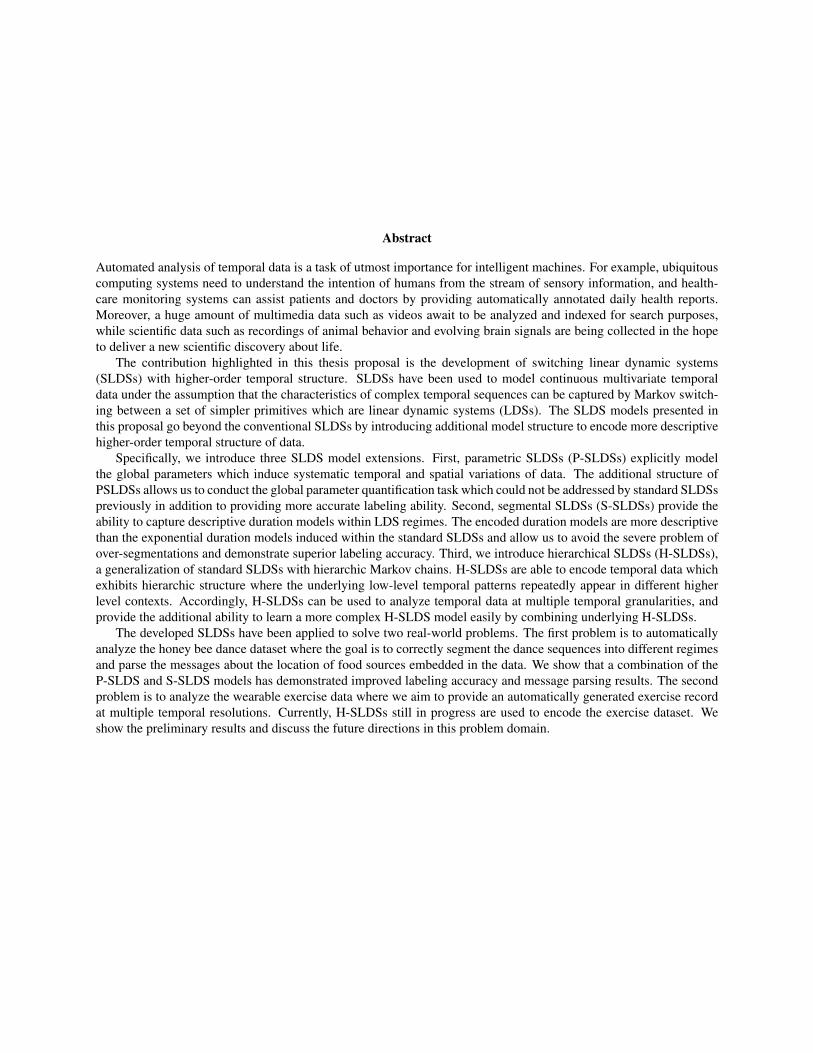
Abstract

Automated analysis of temporal data is a task of utmost importance for intelligent machines. For example, ubiquitouscomputing systems need to understand the intention of humans from the stream of sensory information, and health-care monitoring systems can assist patients and doctors by providing automatically annotated daily health reports.Moreover, a huge amount of multimedia data such as videos await to be analyzed and indexed for search purposes,while scientific data such as recordings of animal behavior and evolving brain signals are being collected in the hopeto deliver a new scientific discovery about life.

The contribution highlighted in this thesis proposal is the development of switching linear dynamic systems(SLDSs) with higher-order temporal structure. SLDSs have been used to model continuous multivariate temporaldata under the assumption that the characteristics of complex temporal sequences can be captured by Markov switch-ing between a set of simpler primitives which are linear dynamic systems (LDSs). The SLDS models presented inthis proposal go beyond the conventional SLDSs by introducing additional model structure to encode more descriptivehigher-order temporal structure of data.

Specifically, we introduce three SLDS model extensions. First, parametric SLDSs (P-SLDSs) explicitly modelthe global parameters which induce systematic temporal and spatial variations of data. The additional structure ofPSLDSs allows us to conduct the global parameter quantification task which could not be addressed by standard SLDSspreviously in addition to providing more accurate labeling ability. Second, segmental SLDSs (S-SLDSs) provide theability to capture descriptive duration models within LDS regimes. The encoded duration models are more descriptivethan the exponential duration models induced within the standard SLDSs and allow us to avoid the severe problem ofover-segmentations and demonstrate superior labeling accuracy. Third, we introduce hierarchical SLDSs (H-SLDSs),a generalization of standard SLDSs with hierarchic Markov chains. H-SLDSs are able to encode temporal data whichexhibits hierarchic structure where the underlying low-level temporal patterns repeatedly appear in different higherlevel contexts. Accordingly, H-SLDSs can be used to analyze temporal data at multiple temporal granularities, andprovide the additional ability to learn a more complex H-SLDS model easily by combining underlying H-SLDSs.

The developed SLDSs have been applied to solve two real-world problems. The first problem is to automaticallyanalyze the honey bee dance dataset where the goal is to correctly segment the dance sequences into different regimesand parse the messages about the location of food sources embedded in the data. We show that a combination of theP-SLDS and S-SLDS models has demonstrated improved labeling accuracy and message parsing results. The secondproblem is to analyze the wearable exercise data where we aim to provide an automatically generated exercise recordat multiple temporal resolutions. Currently, H-SLDSs still in progress are used to encode the exercise dataset. Weshow the preliminary results and discuss the future directions in this problem domain.

Chapter 1

Introduction

The proposed thesis in this research proposal is the following :

“Switching linear dynamic systems with higher-order temporal structure demonstrate superior accuracyover the standard SLDSs for the labeling, classification, and quantification of time-series data ”

In the following sections, we describe the core problems in temporal sequence analysis, our approach towards theproblems, and how it advances the state of the art in this field.

1.1 Automated Temporal Sequence AnalysisTemporal sequences are abundant. Examples of temporal data include motion trajectories, voice, video frames, med-ical sensor signals (e.g., fMRI signals), wearable sensor data, and economic indices, only to name a few. Temporaldata in the most general form is a sequence of multivariate vectors.

In contrast to the abundance of temporal data, the analysis still often relies on the manual interpretation by humans.The manual interpretation of the temporal data, which is a time-consuming process, seems very challenging in somecases due to the complexity of data. For example, sound technicians study complex sound waves, medical doctorsconduct diagnosis based on the signals recorded from medical monitoring systems, and investment bank analystsanalyze the stock price history. In other occasions, the tasks seem simpler, but, the data has still been interpretedand labeled by humans, simply due to the lack of automated analysis tools. For example, computer graphics expertsin animation industry often search for a particular motion sequence from a database investing substantial amount oftime, and field biologists label the tracked motion sequences of animals w.r.t. the corresponding motion regimes byexhaustively examining the tracks frame by frame.

We can observe that the development of automated tools to analyze the temporal sequences can contribute tosuch diverse fields where they would assist the knowledge workers to improve their work productivity through theautomation of diverse manual works. Moreover, these new tools can provide them with the ability to explore a largetemporal sequence database, which was previously challenging due to the substantial amount of manual work required.In addition, the advances in temporal sequence analysis can contribute to so-called emerging real-time applicationswhich are targeted to proactively respond to the needs of the users based on the sensor signals, e.g., medical monitoringdevices and wearable gesture recognition system among many others. Such systems are designed to improve thequality of people’s lives by allowing them to have the necessary assistance at all times and help them to conduct theirtasks more easily.

Among numerous tasks in temporal data analysis domain, we will focus our attention to the following tasks inthis thesis proposal : labeling, quantification, and classification, which we describe more in detail in the followingsections.

LabelingLabeling is the task of categorizing every part of sequences into different classes based on the properties it exhibits.Labeling of temporal sequences is a common task that appears in many fields. The classes can be defined by the

1

(a) (b) (c)

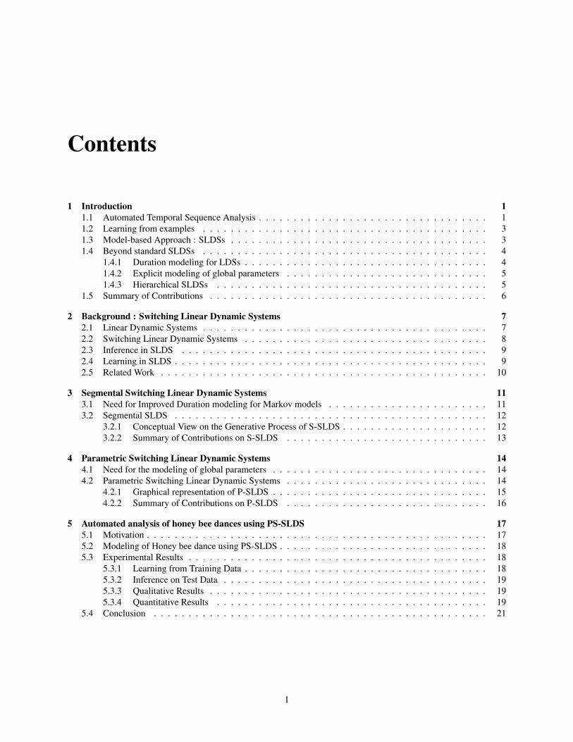
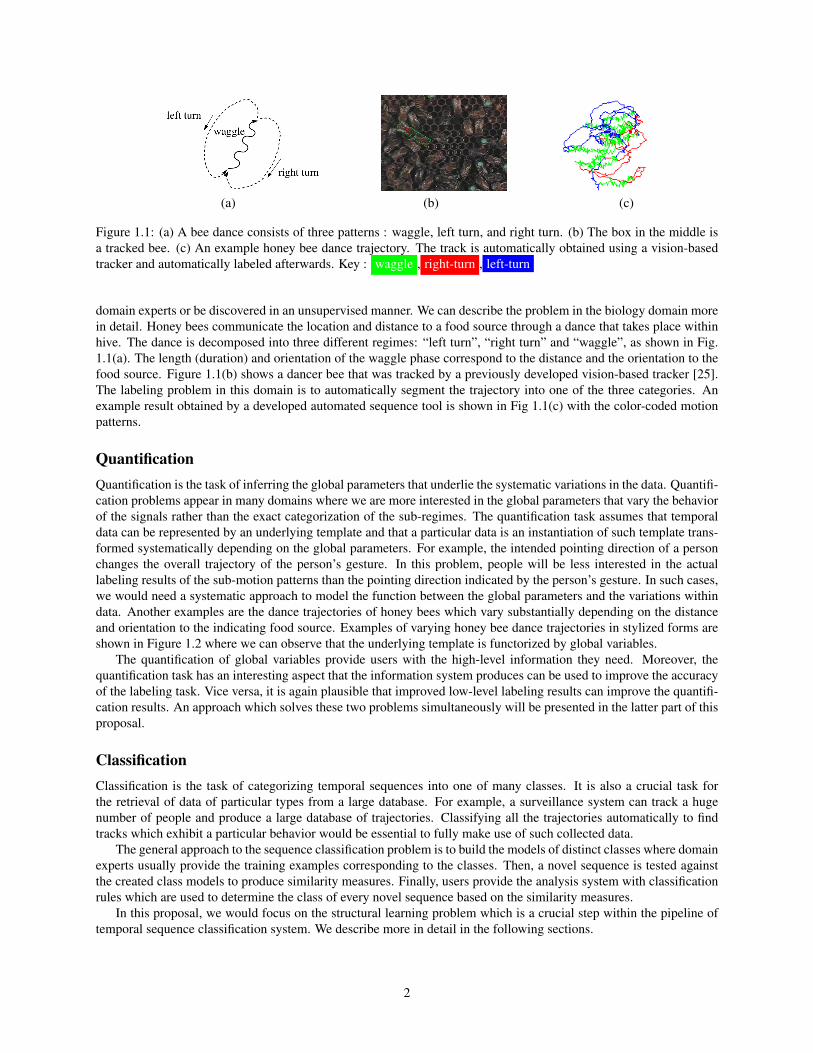
Figure 1.1: (a) A bee dance consists of three patterns : waggle, left turn, and right turn. (b) The box in the middle isa tracked bee. (c) An example honey bee dance trajectory. The track is automatically obtained using a vision-basedtracker and automatically labeled afterwards. Key : waggle , right-turn , left-turn

domain experts or be discovered in an unsupervised manner. We can describe the problem in the biology domain morein detail. Honey bees communicate the location and distance to a food source through a dance that takes place withinhive. The dance is decomposed into three different regimes: “left turn”, “right turn” and “waggle”, as shown in Fig.1.1(a). The length (duration) and orientation of the waggle phase correspond to the distance and the orientation to thefood source. Figure 1.1(b) shows a dancer bee that was tracked by a previously developed vision-based tracker [25].The labeling problem in this domain is to automatically segment the trajectory into one of the three categories. Anexample result obtained by a developed automated sequence tool is shown in Fig 1.1(c) with the color-coded motionpatterns.

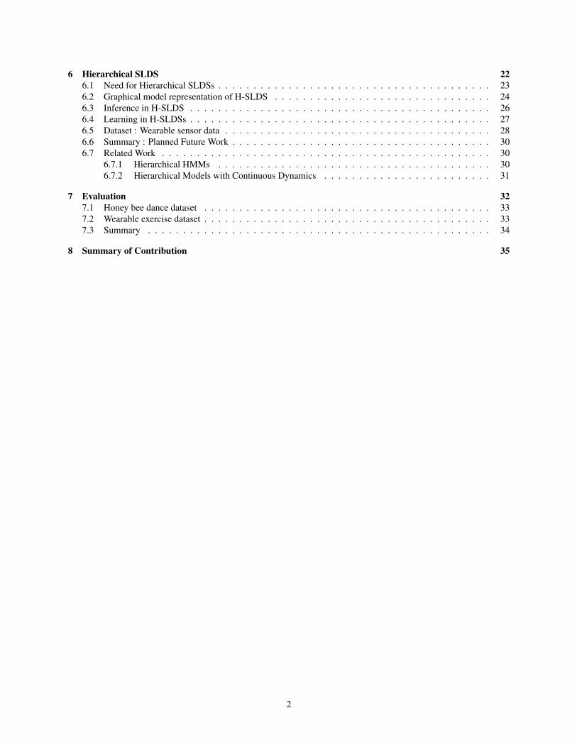
QuantificationQuantification is the task of inferring the global parameters that underlie the systematic variations in the data. Quantifi-cation problems appear in many domains where we are more interested in the global parameters that vary the behaviorof the signals rather than the exact categorization of the sub-regimes. The quantification task assumes that temporaldata can be represented by an underlying template and that a particular data is an instantiation of such template trans-formed systematically depending on the global parameters. For example, the intended pointing direction of a personchanges the overall trajectory of the person’s gesture. In this problem, people will be less interested in the actuallabeling results of the sub-motion patterns than the pointing direction indicated by the person’s gesture. In such cases,we would need a systematic approach to model the function between the global parameters and the variations withindata. Another examples are the dance trajectories of honey bees which vary substantially depending on the distanceand orientation to the indicating food source. Examples of varying honey bee dance trajectories in stylized forms areshown in Figure 1.2 where we can observe that the underlying template is functorized by global variables.

The quantification of global variables provide users with the high-level information they need. Moreover, thequantification task has an interesting aspect that the information system produces can be used to improve the accuracyof the labeling task. Vice versa, it is again plausible that improved low-level labeling results can improve the quantifi-cation results. An approach which solves these two problems simultaneously will be presented in the latter part of thisproposal.

ClassificationClassification is the task of categorizing temporal sequences into one of many classes. It is also a crucial task forthe retrieval of data of particular types from a large database. For example, a surveillance system can track a hugenumber of people and produce a large database of trajectories. Classifying all the trajectories automatically to findtracks which exhibit a particular behavior would be essential to fully make use of such collected data.

The general approach to the sequence classification problem is to build the models of distinct classes where domainexperts usually provide the training examples corresponding to the classes. Then, a novel sequence is tested againstthe created class models to produce similarity measures. Finally, users provide the analysis system with classificationrules which are used to determine the class of every novel sequence based on the similarity measures.

In this proposal, we would focus on the structural learning problem which is a crucial step within the pipeline oftemporal sequence classification system. We describe more in detail in the following sections.

2

Figure 1.2: Examples of various honey bee dance trajectories in stylized forms. The upper row shows the trajectoryvariations which depend on the duration of the waggle phase. The bottom row shows the trajectory variations whichdepend on the orientation of the waggle phase. Waggle phase and angle indicate the distance and orientation to thefood source.

1.2 Learning from examplesThe tasks of labeling, quantification, and classification associate learning problems. Class description, underlyingtemporal templates, the function between global parameters and the template, similarity measures, and classificationrules are often not available even to the domain experts. Hence, it is unlikely that a knowledge engineer who tries todesign an automated analysis system but unfamiliar with the data would possess any such description. In such cases,the task of learning the characteristics of the data from the provided examples becomes the crucial step to build aworking system.

To solve the associated learning problem, we adopt a divide and conquer approach where we assume the followingproperties for the multivariate temporal sequences :

1. Temporal sequences consists of multiple primitive patterns

2. The temporal ordering structure of the primitives provide the characteristic signature of time-series data.

A learning system built under such assumption should have the following functionalities :

1. The system should be able to learn the distinct characteristics of the primitive temporal patterns. In the casewhere the primitive patterns are obvious and labeled examples are available, we would adopt supervised learningapproach. Otherwise, the system should be able to discover the repetitive primitive patterns in an unsupervisedmanner.

2. The system should be able to learn the temporal ordering structures of the primitives across time. The learnedstructures are important parts of the class signatures which can be used to encode the patterns of different classesof sequences.

Accordingly, we would propose a model-based approach where the proposed model consists of sub-models whichswitch over time with a certain temporal ordering structure.

1.3 Model-based Approach : SLDSsWe adopt a model-based approach to characterize temporal sequences. In other words, parametric models are builtfrom training sequences, and used to analyze novel temporal sequences. The basic generative model we adopt is theswitching linear dynamic system (SLDS) model. The SLDS model assumes that complex temporal sequences canbe described by the Markov switching between a set of simpler primitives which are linear dynamic systems (LDSs),often called a Kalman filter models. Hence, the distinctive feature of SLDSs is the fact that they use LDSs as theirprimitives, compared to the piecewise constant approximators used by the popular hidden Markov models (HMMs)[48].

LDS primitives have potential advantages over piecewise constant approximators of HMMs in several aspects.First, LDSs can be more descriptive and concise for diverse types of temporal sequences. Every LDS encodes the

3

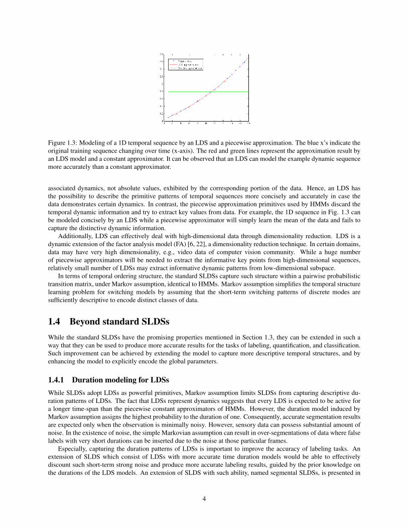
Figure 1.3: Modeling of a 1D temporal sequence by an LDS and a piecewise approximation. The blue x’s indicate theoriginal training sequence changing over time (x-axis). The red and green lines represent the approximation result byan LDS model and a constant approximator. It can be observed that an LDS can model the example dynamic sequencemore accurately than a constant approximator.

associated dynamics, not absolute values, exhibited by the corresponding portion of the data. Hence, an LDS hasthe possibility to describe the primitive patterns of temporal sequences more concisely and accurately in case thedata demonstrates certain dynamics. In contrast, the piecewise approximation primitives used by HMMs discard thetemporal dynamic information and try to extract key values from data. For example, the 1D sequence in Fig. 1.3 canbe modeled concisely by an LDS while a piecewise approximator will simply learn the mean of the data and fails tocapture the distinctive dynamic information.

Additionally, LDS can effectively deal with high-dimensional data through dimensionality reduction. LDS is adynamic extension of the factor analysis model (FA) [6, 22], a dimensionality reduction technique. In certain domains,data may have very high dimensionality, e.g., video data of computer vision community. While a huge numberof piecewise approximators will be needed to extract the informative key points from high-dimensional sequences,relatively small number of LDSs may extract informative dynamic patterns from low-dimensional subspace.

In terms of temporal ordering structure, the standard SLDSs capture such structure within a pairwise probabilistictransition matrix, under Markov assumption, identical to HMMs. Markov assumption simplifies the temporal structurelearning problem for switching models by assuming that the short-term switching patterns of discrete modes aresufficiently descriptive to encode distinct classes of data.

1.4 Beyond standard SLDSsWhile the standard SLDSs have the promising properties mentioned in Section 1.3, they can be extended in such away that they can be used to produce more accurate results for the tasks of labeling, quantification, and classification.Such improvement can be achieved by extending the model to capture more descriptive temporal structures, and byenhancing the model to explicitly encode the global parameters.

1.4.1 Duration modeling for LDSsWhile SLDSs adopt LDSs as powerful primitives, Markov assumption limits SLDSs from capturing descriptive du-ration patterns of LDSs. The fact that LDSs represent dynamics suggests that every LDS is expected to be active fora longer time-span than the piecewise constant approximators of HMMs. However, the duration model induced byMarkov assumption assigns the highest probability to the duration of one. Consequently, accurate segmentation resultsare expected only when the observation is minimally noisy. However, sensory data can possess substantial amount ofnoise. In the existence of noise, the simple Markovian assumption can result in over-segmentations of data where falselabels with very short durations can be inserted due to the noise at those particular frames.

Especially, capturing the duration patterns of LDSs is important to improve the accuracy of labeling tasks. Anextension of SLDS which consist of LDSs with more accurate time duration models would be able to effectivelydiscount such short-term strong noise and produce more accurate labeling results, guided by the prior knowledge onthe durations of the LDS models. An extension of SLDS with such ability, named segmental SLDSs, is presented in

4

Chapter 3as one of the contributions of this proposal work.

1.4.2 Explicit modeling of global parametersThe standard SLDS does not provide a principled way to model the parameterized temporal sequences, i.e., the datawhich exhibits systematic temporal and spatial variations. We adopt an approach where we explicitly models the func-tion which deforms the underlying canonical template based on the global parameters to produce data with systematicvariations. An illustrative example is the honeybee dances : bees communicate the orientation and the distance to thefood sources through the dance angles and waggle duration of their stylized dances. In this example, the canonicalunderlying template is in the form of the prototype dance trajectory illustrated in Fig. 1.1 (a), and the resulting exampletrajectories are shown in Fig. 1.2.

We introduce a new representation for the class of parameterized multivariate temporal sequences : parametricSLDSs (P-SLDS). Our work is partly inspired by the previous work of Wilson & Bobick where they presented para-metric HMMs [59], an extension to HMMs with which they successfully interpreted human gestures. As in P-HMMs,the P-SLDS model incorporates global parameters that underlay systematic spatial variations of the overall target mo-tion. In addition, while P-HMMs only introduced global observation parameters which describe spatial variations inthe outputs, we additionally introduce dynamic parameters which capture temporal variations. As mentioned earlier,the problems of global parameter quantification and labeling can be solved simultaneously. Hence, we formulateexpectation-maximization (EM) methods for learning and inference in P-SLDS and present it in Chapter 4 of thisthesis proposal.

1.4.3 Hierarchical SLDSsWe propose to address the learning of a hierarchical extension of SLDSs as a future work of this proposed research.The use of the hierarchical models for the automated temporal sequence analysis instead of the flat Markov modelsis motivated by the fact that hierarchical models can capture the correlations between the events appearing far apartin the sequence, while flat Markov models can only capture the local correlations. Additionally, hierarchical modelseven provide the ability to encode the repetitive patterns more precisely than the flat Markov models which tend tolearn the averaged switching patterns.

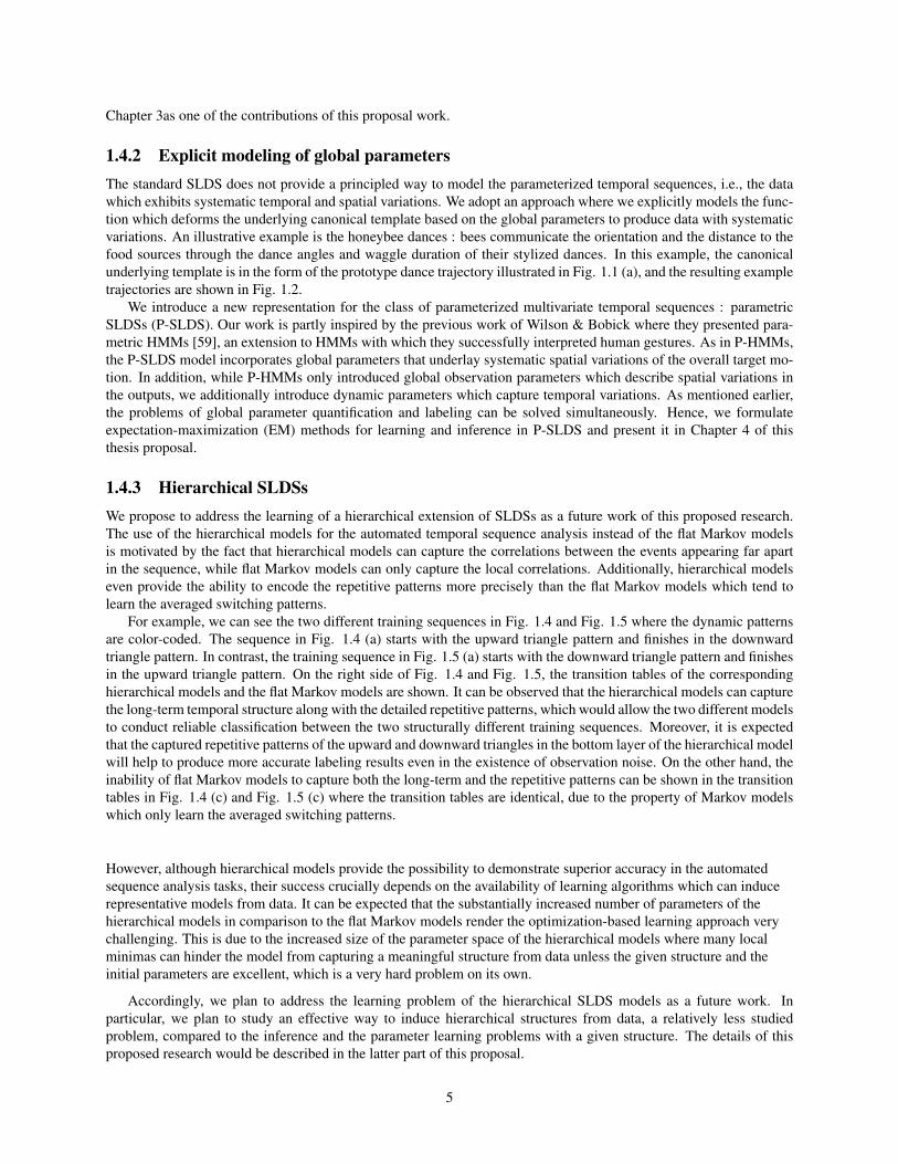
For example, we can see the two different training sequences in Fig. 1.4 and Fig. 1.5 where the dynamic patternsare color-coded. The sequence in Fig. 1.4 (a) starts with the upward triangle pattern and finishes in the downwardtriangle pattern. In contrast, the training sequence in Fig. 1.5 (a) starts with the downward triangle pattern and finishesin the upward triangle pattern. On the right side of Fig. 1.4 and Fig. 1.5, the transition tables of the correspondinghierarchical models and the flat Markov models are shown. It can be observed that the hierarchical models can capturethe long-term temporal structure along with the detailed repetitive patterns, which would allow the two different modelsto conduct reliable classification between the two structurally different training sequences. Moreover, it is expectedthat the captured repetitive patterns of the upward and downward triangles in the bottom layer of the hierarchical modelwill help to produce more accurate labeling results even in the existence of observation noise. On the other hand, theinability of flat Markov models to capture both the long-term and the repetitive patterns can be shown in the transitiontables in Fig. 1.4 (c) and Fig. 1.5 (c) where the transition tables are identical, due to the property of Markov modelswhich only learn the averaged switching patterns.

However, although hierarchical models provide the possibility to demonstrate superior accuracy in the automatedsequence analysis tasks, their success crucially depends on the availability of learning algorithms which can inducerepresentative models from data. It can be expected that the substantially increased number of parameters of thehierarchical models in comparison to the flat Markov models render the optimization-based learning approach verychallenging. This is due to the increased size of the parameter space of the hierarchical models where many localminimas can hinder the model from capturing a meaningful structure from data unless the given structure and theinitial parameters are excellent, which is a very hard problem on its own.

Accordingly, we plan to address the learning problem of the hierarchical SLDS models as a future work. Inparticular, we plan to study an effective way to induce hierarchical structures from data, a relatively less studiedproblem, compared to the inference and the parameter learning problems with a given structure. The details of thisproposed research would be described in the latter part of this proposal.

5

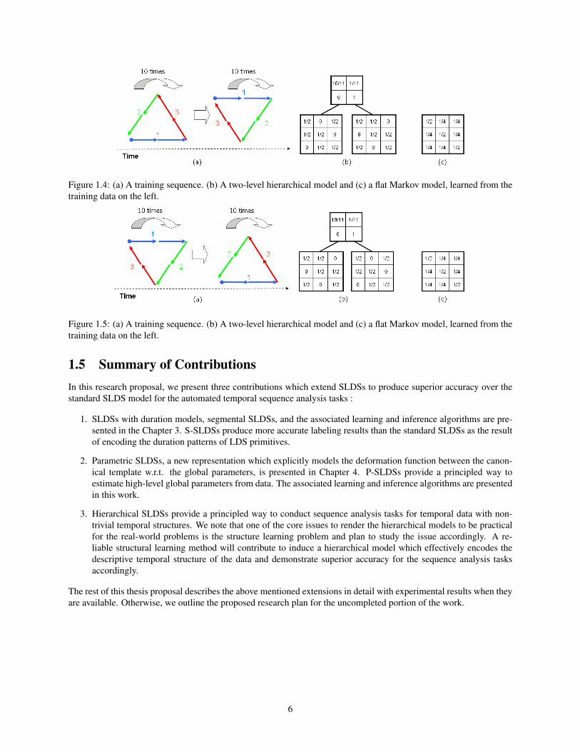
Figure 1.4: (a) A training sequence. (b) A two-level hierarchical model and (c) a flat Markov model, learned from thetraining data on the left.

Figure 1.5: (a) A training sequence. (b) A two-level hierarchical model and (c) a flat Markov model, learned from thetraining data on the left.

1.5 Summary of ContributionsIn this research proposal, we present three contributions which extend SLDSs to produce superior accuracy over thestandard SLDS model for the automated temporal sequence analysis tasks :

1. SLDSs with duration models, segmental SLDSs, and the associated learning and inference algorithms are pre-sented in the Chapter 3. S-SLDSs produce more accurate labeling results than the standard SLDSs as the resultof encoding the duration patterns of LDS primitives.

2. Parametric SLDSs, a new representation which explicitly models the deformation function between the canon-ical template w.r.t. the global parameters, is presented in Chapter 4. P-SLDSs provide a principled way toestimate high-level global parameters from data. The associated learning and inference algorithms are presentedin this work.

3. Hierarchical SLDSs provide a principled way to conduct sequence analysis tasks for temporal data with non-trivial temporal structures. We note that one of the core issues to render the hierarchical models to be practicalfor the real-world problems is the structure learning problem and plan to study the issue accordingly. A re-liable structural learning method will contribute to induce a hierarchical model which effectively encodes thedescriptive temporal structure of the data and demonstrate superior accuracy for the sequence analysis tasksaccordingly.

The rest of this thesis proposal describes the above mentioned extensions in detail with experimental results when theyare available. Otherwise, we outline the proposed research plan for the uncompleted portion of the work.

6

Chapter 2

Background : Switching Linear DynamicSystems

Switching Linear Dynamic System (SLDS) models have been studied in a variety of problem domains. Representativeexamples include computer vision [46, 45, 47, 38, 9, 42], computer graphics [32, 49], control systems [58], economet-rics [26], speech recognition [44, 50] (Jeff Ma paper add), tracking [5], machine learning [30, 21, 40, 39, 24], signalprocessing [15, 16], statistics [55] and visualization [60]. While there are several versions of SLDS in the literature,this paper addresses the model structure depicted in Figure 2.2.

An SLDS model represents the nonlinear dynamic behavior of a complex system by switching among a set oflinear dynamic models over time. In contrast to HMM’s [48], the Markov process in an SLDS selects from a set ofcontinuously-evolving linear Gaussian dynamics, rather than a fixed Gaussian mixture density. As a consequence, anSLDS has potentially greater descriptive power. Offsetting this advantage is the fact that exact inference in an SLDS isintractable in case the continuous states are coupled during the switchings, which complicates inference and parameterlearning [29].

The rest of this chapter is organized as follows. First, we review the linear dynamic systems (LDSs), and itsextension, switching LDSs (SLDSs). Then, we review a set of the developed approximate inference techniques and anEM-based learning method for SLDSs. Finally, related work is reviewed and this chapter concludes.

2.1 Linear Dynamic Systems

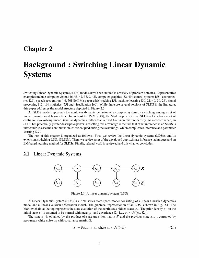
Figure 2.1: A linear dynamic system (LDS)

A Linear Dynamic System (LDS) is a time-series state-space model consisting of a linear Gaussian dynamicsmodel and a linear Gaussian observation model. The graphical representation of an LDS is shown in Fig. 2.1. TheMarkov chain at the top represents the state evolution of the continuous hidden states xt. The prior density p1 on theinitial state x1 is assumed to be normal with mean µ1 and covariance Σ1, i.e., x1 ∼ N (µ1,Σ1).

The state xt is obtained by the product of state transition matrix F and the previous state xt−1, corrupted byzero-mean white noise wt with covariance matrix Q:

xt = Fxt−1 + wt where wt ∼ N (0, Q) (2.1)

7

In addition, the measurement zt is generated from the current state xt through the observation matrix H , and corruptedby zero-mean observation noise vt:

zt = Hxt + vt where vt ∼ N (0, V ) (2.2)

Thus, an LDS model M is defined by the tuple M∆= {(µ1,Σ1), (F,Q), (H,V )}. Exact inference in an LDS can be

performed using the RTS smoother [4], an efficient variant of belief propagation for linear Gaussian models. Furtherdetails on LDSs can be found in [4, 33, 51].

Linear dynamic system has been often used for tracking problems [4, 33]. In addition, LDSs have been used tomodel the overall texture of the video scenes in a compact way with the video as a sequence of observations andgenerate a infinitely long video similar to the training sequences [14]. In other work, multiple LDSs were used tosegment video w.r.t. the associated temporal texture patterns [11].

2.2 Switching Linear Dynamic Systems

Figure 2.2: Switching linear dynamic systems (SLDS)

In a switching LDSs (SLDSs), we assume the existence of n distinct LDS models M∆= {Ml|1 ≤ l ≤ n}. The

graphical model corresponding to an SLDS is shown in Fig. 2.2. The middle chain, representing the hidden statesequence X

∆= {xt|1 ≤ t ≤ T}, together with the observations Z∆= {zt|1 ≤ t ≤ T} at the bottom, is identical to an

LDS in Fig. 2.1. However, we now have an additional discrete Markov chain L∆= {lt|1 ≤ t ≤ T} that determines

which of the n models Ml is used at every time-step. We call lt ∈M the label at time t and L a label sequence.The switching state lt is obtained from the previous state label lt−1 based on the Markov transition model P (lt|lt−1, B)

which is represented as an n × n transition matrix B that defines the switching behavior between the n distinct LDSmodels :

lt ∼ P (lt|lt−1, B) (2.3)

The state xt is obtained by the product of the corresponding state transition matrix Flt and the previous state xt−1,corrupted by zero-mean white noise wt with covariance matrix Qlt :

xt = Fltxt−1 + wt where wt ∼ N (0, Qlt) (2.4)

In addition, the measurement zt is generated from the current state xt through the corresponding observation matrixHlt , and corrupted by zero-mean observation noise vt with covariance Vlt :

zt = Hltxt + vt where vt ∼ N (0, Vlt) (2.5)

Finally, in addition to a set of LDS models M , we specify two additional parameters: a multinomial distributionπ(l1) over the initial label l1 :

l1 ∼ π(l1) (2.6)

8

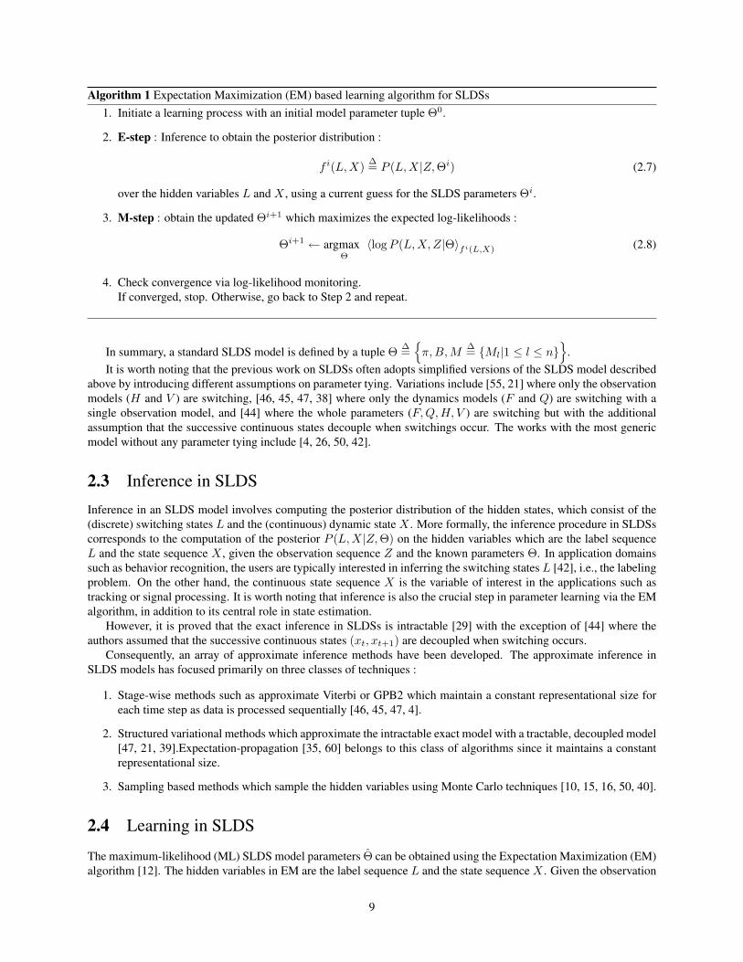
Algorithm 1 Expectation Maximization (EM) based learning algorithm for SLDSs1. Initiate a learning process with an initial model parameter tuple Θ0.

2. E-step : Inference to obtain the posterior distribution :

f i(L,X) ∆= P (L,X|Z,Θi) (2.7)

over the hidden variables L and X , using a current guess for the SLDS parameters Θi.

3. M-step : obtain the updated Θi+1 which maximizes the expected log-likelihoods :

Θi+1 ← argmaxΘ

〈log P (L,X, Z|Θ〉fi(L,X) (2.8)

4. Check convergence via log-likelihood monitoring.If converged, stop. Otherwise, go back to Step 2 and repeat.

In summary, a standard SLDS model is defined by a tuple Θ ∆={

π,B,M∆= {Ml|1 ≤ l ≤ n}

}.

It is worth noting that the previous work on SLDSs often adopts simplified versions of the SLDS model describedabove by introducing different assumptions on parameter tying. Variations include [55, 21] where only the observationmodels (H and V ) are switching, [46, 45, 47, 38] where only the dynamics models (F and Q) are switching with asingle observation model, and [44] where the whole parameters (F,Q,H, V ) are switching but with the additionalassumption that the successive continuous states decouple when switchings occur. The works with the most genericmodel without any parameter tying include [4, 26, 50, 42].

2.3 Inference in SLDS

Inference in an SLDS model involves computing the posterior distribution of the hidden states, which consist of the(discrete) switching states L and the (continuous) dynamic state X . More formally, the inference procedure in SLDSscorresponds to the computation of the posterior P (L,X|Z,Θ) on the hidden variables which are the label sequenceL and the state sequence X , given the observation sequence Z and the known parameters Θ. In application domainssuch as behavior recognition, the users are typically interested in inferring the switching states L [42], i.e., the labelingproblem. On the other hand, the continuous state sequence X is the variable of interest in the applications such astracking or signal processing. It is worth noting that inference is also the crucial step in parameter learning via the EMalgorithm, in addition to its central role in state estimation.

However, it is proved that the exact inference in SLDSs is intractable [29] with the exception of [44] where theauthors assumed that the successive continuous states (xt, xt+1) are decoupled when switching occurs.

Consequently, an array of approximate inference methods have been developed. The approximate inference inSLDS models has focused primarily on three classes of techniques :

1. Stage-wise methods such as approximate Viterbi or GPB2 which maintain a constant representational size foreach time step as data is processed sequentially [46, 45, 47, 4].

2. Structured variational methods which approximate the intractable exact model with a tractable, decoupled model[47, 21, 39].Expectation-propagation [35, 60] belongs to this class of algorithms since it maintains a constantrepresentational size.

3. Sampling based methods which sample the hidden variables using Monte Carlo techniques [10, 15, 16, 50, 40].

2.4 Learning in SLDS

The maximum-likelihood (ML) SLDS model parameters Θ can be obtained using the Expectation Maximization (EM)algorithm [12]. The hidden variables in EM are the label sequence L and the state sequence X . Given the observation

9

data Z, EM proceeds as described in Algorithm 1.Above, 〈·〉W denotes the expectation of a function (·) under a distribution W . The E-step in Eq. 2.7 corresponds

to the inference procedure for SLDSs. As mentioned in Section 2.3, it is proved that the exact inference in SLDSs isintractable [29]. Hence, we should rely on one of the approximate inference methods described in Section 2.3 for theE-step, unless we use the variation in [44].

The learning procedure in Algorithm 1 is simplified in the case where the ground truth LDS labels for the trainingsequences are known. In that case, every LDS parameters are learned separately based on the corresponding parts ofthe data. Then, the parameters of the discrete process, initial distribution π(l1) and the Markov switching matrix B,are learned separately.

On the other hand, if the ground truth labels are unavailable, the underlying LDS models should be learned in anunsupervised way. In that case, the inferred labels in Algorithm 1 are used to partition the data which provide the basisto learn distinct LDS models.

2.5 Related WorkThe development of SLDSs is closely related with the work on dimensionality reduction [57, 52, 22] for static (nontime-series) data as well. In particular, the SLDS model can be thought to be a dynamic parallel of the work onmodeling complex static dataset as a mixture of low-dimensional linear models [57, 22]. This analogy can be madesince SLDSs aim to model non-linear and high dimensional data as the mixtures of locally linear dynamic systemswhich switch over time in the latent space.

10

Chapter 3

Segmental Switching Linear DynamicSystems

3.1 Need for Improved Duration modeling for Markov models

The duration modeling capability of any first-order Markov model is limited by its own assumption upon the transitionsbetween the discrete switching states. As a consequence of Markov assumption, the probability of remaining in a givenswitching state follows a geometric distribution :

P (d) = ad−1(1− a) (3.1)

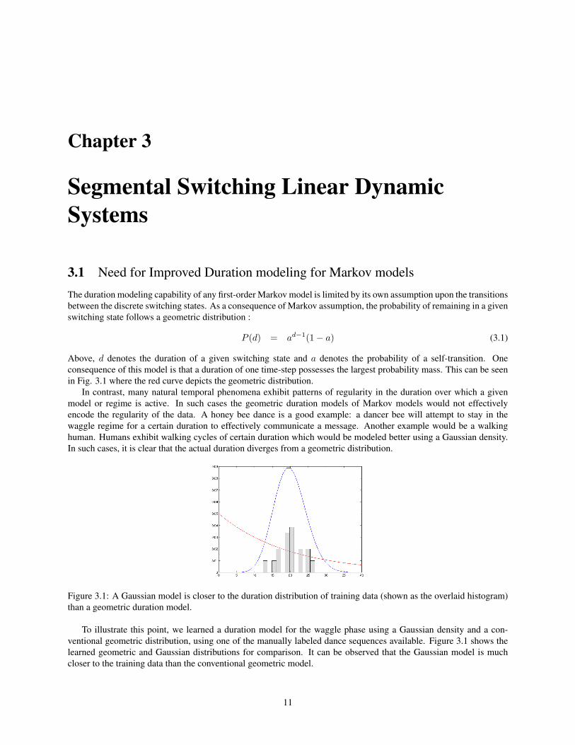
Above, d denotes the duration of a given switching state and a denotes the probability of a self-transition. Oneconsequence of this model is that a duration of one time-step possesses the largest probability mass. This can be seenin Fig. 3.1 where the red curve depicts the geometric distribution.

In contrast, many natural temporal phenomena exhibit patterns of regularity in the duration over which a givenmodel or regime is active. In such cases the geometric duration models of Markov models would not effectivelyencode the regularity of the data. A honey bee dance is a good example: a dancer bee will attempt to stay in thewaggle regime for a certain duration to effectively communicate a message. Another example would be a walkinghuman. Humans exhibit walking cycles of certain duration which would be modeled better using a Gaussian density.In such cases, it is clear that the actual duration diverges from a geometric distribution.

Figure 3.1: A Gaussian model is closer to the duration distribution of training data (shown as the overlaid histogram)than a geometric duration model.

To illustrate this point, we learned a duration model for the waggle phase using a Gaussian density and a con-ventional geometric distribution, using one of the manually labeled dance sequences available. Figure 3.1 shows thelearned geometric and Gaussian distributions for comparison. It can be observed that the Gaussian model is muchcloser to the training data than the conventional geometric model.

11

The limitation of a geometric distribution has been previously addressed by the HMM, and HMM models withenhanced duration capabilities have been developed [17, 31, 53, 44]. The variable duration HMM (VD-HMM) wasintroduced in [17] : state durations are modeled explicitly in a variety of PDF forms. Later, a different parameterizationof the state durations was introduced where the state transition probabilities are modeled as functions of time, whichare referred to as non-stationary HMMs (NS-HMM) [31]. It has since been shown that the VD-HMM and the NS-HMM are duals [13]. In addition, segmental HMM with random effects was developed in the data mining community[20, 27]. Ostendorf et.al. provide an excellent discussion of segmental HMMs in [44].

We adopt similar ideas to arrive at SLDS models with enhanced duration modeling.

3.2 Segmental SLDS

We introduce the segmental SLDS (S-SLDS) model, which improves upon the standard SLDS model by relaxing theMarkov assumption at a time-step level to a coarser segment level. The development of the S-SLDS model is motivatedby the regularity in durations that is often exhibited in nature. For example, as discussed in Section 3.1, a dancer beewill attempt to stay in the waggle regime for a certain duration to effectively communicate the distance to the foodsource. In such a case, the geometric distribution induced in a standard SLDS is not an appropriate choice. Fig. 3.1shows that a geometric distribution assigns the highest probability to the duration of a single time step. As a result, thelabel inference in standard SLDSs is susceptible to over-segmentation.

In an S-SLDS, the durations are first modeled explicitly [17] and then non-stationary duration functions [31] arederived from them. Both of them are learned from data. As a consequence, the S-SLDS model has more descriptivepower and can yield more accurate results than the standard SLDSs. Nonetheless, we show that one can always converta learned S-SLDS model into an equivalent standard SLDS, operating in a different label space. The approach hasthe significant advantage of allowing us to reuse the large array of approximate inference and learning techniquesdeveloped for SLDSs.

3.2.1 Conceptual View on the Generative Process of S-SLDS

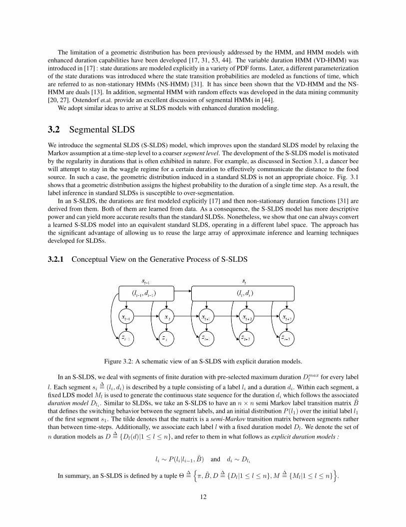
Figure 3.2: A schematic view of an S-SLDS with explicit duration models.

In an S-SLDS, we deal with segments of finite duration with pre-selected maximum duration Dmaxl for every label

l. Each segment si∆= (li, di) is described by a tuple consisting of a label li and a duration di. Within each segment, a

fixed LDS model Ml is used to generate the continuous state sequence for the duration di which follows the associatedduration model Dli . Similar to SLDSs, we take an S-SLDS to have an n × n semi Markov label transition matrix Bthat defines the switching behavior between the segment labels, and an initial distribution P (l1) over the initial label l1of the first segment s1. The tilde denotes that the matrix is a semi-Markov transition matrix between segments ratherthan between time-steps. Additionally, we associate each label l with a fixed duration model Dl. We denote the set ofn duration models as D

∆= {Dl(d)|1 ≤ l ≤ n}, and refer to them in what follows as explicit duration models :

li ∼ P (li|li−1, B) and di ∼ Dli

In summary, an S-SLDS is defined by a tuple Θ ∆={

π, B,D∆= {Dl|1 ≤ l ≤ n},M ∆= {Ml|1 ≤ l ≤ n}

}.

12

A schematic depiction of an S-SLDS is illustrated in Fig. 3.2. The top chain in the figure is a series of segmentswhere each segment is depicted as a rounded box. In the model, the current segment si

∆= (li, di) generates a nextsegment si+1 in the following manner: first, the current label li generates the next label li+1 based on the labeltransition matrix B; then, the next duration di+1 is generated from the duration model for the label li+1, i.e. di+1 ∼Dli+1(d). The dynamics for the continuous hidden states and observations are identical to a standard SLDS : a segmentsi evolves the set of continuous hidden states X with a corresponding LDS model Mli for the duration di, then theobservations Z are generated given the labels L and the set of continuous states X .

3.2.2 Summary of Contributions on S-SLDS

The conceptual S-SLDS model described in Section 3.2.1 has been formulated formally within a graphical modelframework [43, 42] where appropriate learning and inference methods are developed. The details of the developedlearning and inference techniques can be summarized as follows :

• Learning method is developed within EM framework.

• Inference method is based on previously developed inference technique for standard SLDSs. Basically, weintroduced a technique to convert an S-SLDS model into a standard SLDS model, and reuse the existing arrayof previously developed inference techniques.

• Techniques to speed-up inference process have been developed. The resulting algorithm has complexity ofO(TDmax|L|2), compared to the complexity O(TD2

max|L|2) resulting from the blind re-use of the existingmethods. For your information, the complexity of the inference techniques for standard SLDS is O(T |L|2).

For more details, please refer to the published work [43, 42].

13

Chapter 4

Parametric Switching Linear DynamicSystems

4.1 Need for the modeling of global parameters

Temporal sequences are often parameterized by global factors. For example, people walk, but at different paces andwith different styles. Sound fluctuates, but with different frequencies and different amplitudes. Hence, one importantproblem in temporal sequence analysis is ’quantification’, by which we mean the identification of global parametersthat underlay the behavior of the signals, e.g., the direction of a pointing gesture. However, most switching systemmodels are only designed to be able to label the temporal sequences into different regimes, e.g., HMMs or SLDSs.Nonetheless, these two inference tasks are not independent : a better understanding on the systematic variations in thedata can improve labeling results, and vice versa. A speech recognition system which is aware of the general utterancepattern of a specific person would be able to recognize the speech of that person more accurately.

The consideration of global parameters is motivated by two observations : (1) temporal sequences can be oftendescribed as the combination of a representative template and underlying global variations, and (2) we are often moreinterested in estimating the global parameters rather than the exact categorization of the sub-regimes. Unfortunately,the standard SLDS model does not provide a principled way to quantify temporal and spatial variations w.r.t. the fixed(canonical) underlying behavioral template.

Previously, Wilson & Bobick addressed this problem by presenting a parametric HMMs (P-HMM) [59]. In aP-HMM, the parametric observation models learned are conditioned on global observation parameters and globallyparameterized gestures could be recognized. P-HMMs have been used to interpret human gestures and demonstratedsuperior recognition performance in comparison to standard HMMs.

Inspired by P-HMM, we extend the standard SLDS model, resulting in a parametric SLDS (P-SLDS). As in aP-HMM, the P-SLDS model incorporates global parameters that underlay systematic spatial variations of the overalltarget motion, and is able to estimate the associated global parameters from data. In addition, while P-HMMs onlyintroduced global observation parameters which describe the spatial variations in the outputs, we additionally intro-duce global dynamic parameters which capture temporal variations. As mentioned earlier, the problems of globalparameter quantification and labeling can be solved simultaneously. Hence, we formulate expectation-maximization(EM) methods for learning and inference in P-SLDSs and present it in Section 4.2. A preliminary version of P-SLDSwork appeared in [41].

4.2 Parametric Switching Linear Dynamic Systems

As discussed in Section 4.1, the standard SLDS does not provide a principled means to quantify global variations inthe motion patterns. For example, honey bees communicate the orientation and distance to food sources through the(spatial) dance angles and (temporal) waggle durations of their stylized dances which take place in the hive. As aresult, these global motion parameters which encode the message of the bee dance are the variables that we are mostinterested in estimating.

14

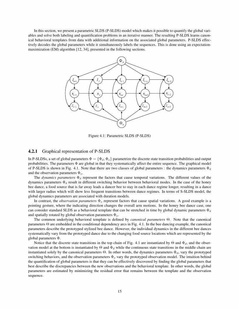
In this section, we present a parametric SLDS (P-SLDS) model which makes it possible to quantify the global vari-ables and solve both labeling and quantification problems in an iterative manner. The resulting P-SLDS learns canon-ical behavioral templates from data with additional information on the associated global parameters. P-SLDS effec-tively decodes the global parameters while it simultaneously labels the sequences. This is done using an expectation-maximization (EM) algorithm [12, 34], presented in the following sections.

Figure 4.1: Parametric SLDS (P-SLDS)

4.2.1 Graphical representation of P-SLDS

In P-SLDSs, a set of global parameters Φ = {Φd,Φo} parametrize the discrete state transition probabilities and outputprobabilities. The parameters Φ are global in that they systematically affect the entire sequence. The graphical modelof P-SLDS is shown in Fig. 4.1. Note that there are two classes of global parameters : the dynamics parameters Φd

and the observation parameters Φo.The dynamics parameters Φd represent the factors that cause temporal variations. The different values of the

dynamics parameters Φd result in different switching behavior between behavioral modes. In the case of the honeybee dance, a food source that is far away leads a dancer bee to stay in each dance regime longer, resulting in a dancewith larger radius which will show less frequent transitions between dance regimes. In terms of S-SLDS model, theglobal dynamics parameters are associated with duration models.

In contrast, the observation parameters Φo represent factors that cause spatial variations. A good example is apointing gesture, where the indicating direction changes the overall arm motions. In the honey bee dance case, onecan consider standard SLDS as a behavioral template that can be stretched in time by global dynamic parameters Φd

and spatially rotated by global observation parameters Φo.The common underlying behavioral template is defined by canonical parameters Θ. Note that the canonical

parameters Θ are embedded in the conditional dependency arcs in Fig. 4.1. In the bee dancing example, the canonicalparameters describe the prototyped stylized bee dance. However, the individual dynamics in the different bee dancessystematically vary from the prototyped dance due to the changing food source locations which are represented by theglobal parameters Φ.

Notice that the discrete state transitions in the top chain of Fig. 4.1 are instantiated by Θ and Φd, and the obser-vation model at the bottom is instantiated by Θ and Φd while the continuous state transitions in the middle chain areinstantiated solely by the canonical parameters Θ. In other words, the dynamics parameters Φd, vary the prototypedswitching behaviors, and the observation parameters Φo vary the prototyped observation model. The intuition behindthe quantification of global parameters is that they can be effectively discovered by finding the global parameters thatbest describe the discrepancies between the new observations and the behavioral template. In other words, the globalparameters are estimated by minimizing the residual error that remains between the template and the observationsequence.

15

The result of parameterizing the SLDS model is the incorporation of additional conditioning variables in theinitial state distribution P (l1|Θ,Φd), the discrete state transition table P (lt|lt−1,Θ,Φd), and the observation modelP (zt|lt, xt,Θ,Φo). There are three possibilities for the nature of the parameterization: (a) the PDF is a linear functionof the global parameters Φ, (b) the PDF is a non-linear function of Φ, and (c) no functional form for the PDF isavailable. In the latter case of (c), general function approximators such as neural network may be used, as suggestedin [59].

4.2.2 Summary of Contributions on P-SLDS

In addition to introducing the graphical model of P-SLDS, appropriate learning and inference methods are developed[41, 42]. The details of the developed learning and inference techniques can be summarized as follows :

• A learning method for P-SLDS model is developed within EM framework. It is assumed that the global param-eters are available as part of the training data, and the functional forms of the parameterization are available.Since the global variables are known, the learning for P-SLDS is often analogous to the learning for standardSLDSs with additional parameters.

• Inference method is based on EM as well. The intuition for EM-based inference method is straightforward. Ourgoal is to find the unknown global parameter settings which maximize the likelihood of the model against thegiven test data. Hence, the inference procedure can be formulated within EM framework by treating the globalparameters as missing variables. With reasonable initial value, it has been observed that the the global variableswere refined through EM iterations and mostly converged to values close to the ground truths.

For more details, please refer to the published work [41, 42].

16

Chapter 5

Automated analysis of honey bee dancesusing PS-SLDS

In this chapter, we evaluate our thesis by applying the developed theory of S-SLDSs developed in Chapter 3, andthe theory of P-SLDSs in Chapter 4 on the real-world honey bee dataset for the labeling and quantification tasks. Totake advantage of both models, we combine the models and use the resulting parametric segmental SLDS (PS-SLDS)model to learn the temporal patterns from data and use the learned model to conduct labeling and quantification tasks.The resulting PS-SLDS model demonstrates superior accuracy over the standard SLDS model for both the labelingand the quantification tasks.

5.1 MotivationThe application domain which motivates the work in this chapter is a new research area which enlists visual trackingand AI modeling techniques in the service of biology [2, 3, 8, 54]. The current state of biological field work is stilldominated by manual data interpretation, a time-consuming process. Automatic interpretation methods can providefield biologists with new tools for the quantitative study of animal behavior.

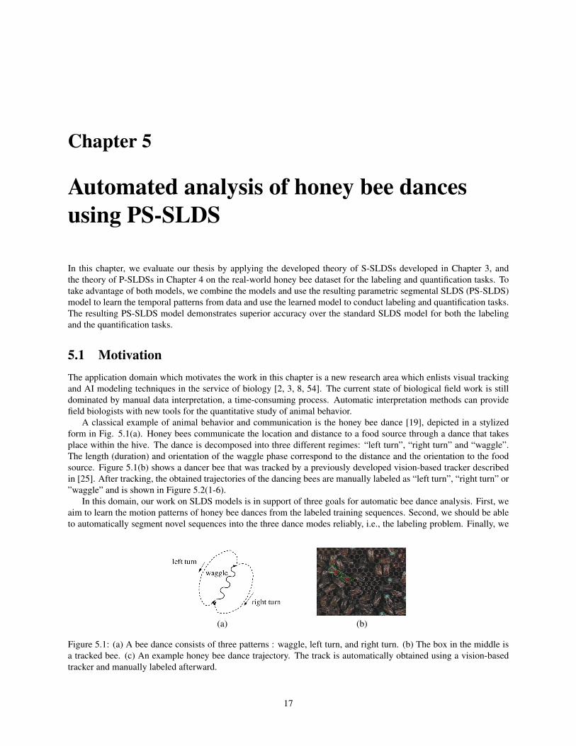
A classical example of animal behavior and communication is the honey bee dance [19], depicted in a stylizedform in Fig. 5.1(a). Honey bees communicate the location and distance to a food source through a dance that takesplace within the hive. The dance is decomposed into three different regimes: “left turn”, “right turn” and “waggle”.The length (duration) and orientation of the waggle phase correspond to the distance and the orientation to the foodsource. Figure 5.1(b) shows a dancer bee that was tracked by a previously developed vision-based tracker describedin [25]. After tracking, the obtained trajectories of the dancing bees are manually labeled as “left turn”, “right turn” or”waggle” and is shown in Figure 5.2(1-6).

In this domain, our work on SLDS models is in support of three goals for automatic bee dance analysis. First, weaim to learn the motion patterns of honey bee dances from the labeled training sequences. Second, we should be ableto automatically segment novel sequences into the three dance modes reliably, i.e., the labeling problem. Finally, we

(a) (b)

Figure 5.1: (a) A bee dance consists of three patterns : waggle, left turn, and right turn. (b) The box in the middle isa tracked bee. (c) An example honey bee dance trajectory. The track is automatically obtained using a vision-basedtracker and manually labeled afterward.

17

(1) (2) (3) (4) (5) (6)

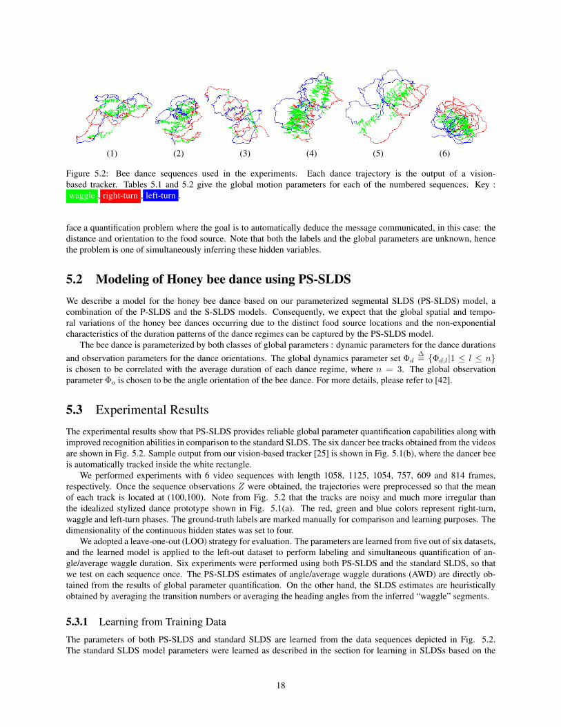
Figure 5.2: Bee dance sequences used in the experiments. Each dance trajectory is the output of a vision-based tracker. Tables 5.1 and 5.2 give the global motion parameters for each of the numbered sequences. Key :waggle , right-turn , left-turn .

face a quantification problem where the goal is to automatically deduce the message communicated, in this case: thedistance and orientation to the food source. Note that both the labels and the global parameters are unknown, hencethe problem is one of simultaneously inferring these hidden variables.

5.2 Modeling of Honey bee dance using PS-SLDSWe describe a model for the honey bee dance based on our parameterized segmental SLDS (PS-SLDS) model, acombination of the P-SLDS and the S-SLDS models. Consequently, we expect that the global spatial and tempo-ral variations of the honey bee dances occurring due to the distinct food source locations and the non-exponentialcharacteristics of the duration patterns of the dance regimes can be captured by the PS-SLDS model.

The bee dance is parameterized by both classes of global parameters : dynamic parameters for the dance durationsand observation parameters for the dance orientations. The global dynamics parameter set Φd

∆= {Φd,l|1 ≤ l ≤ n}is chosen to be correlated with the average duration of each dance regime, where n = 3. The global observationparameter Φo is chosen to be the angle orientation of the bee dance. For more details, please refer to [42].

5.3 Experimental Results

The experimental results show that PS-SLDS provides reliable global parameter quantification capabilities along withimproved recognition abilities in comparison to the standard SLDS. The six dancer bee tracks obtained from the videosare shown in Fig. 5.2. Sample output from our vision-based tracker [25] is shown in Fig. 5.1(b), where the dancer beeis automatically tracked inside the white rectangle.

We performed experiments with 6 video sequences with length 1058, 1125, 1054, 757, 609 and 814 frames,respectively. Once the sequence observations Z were obtained, the trajectories were preprocessed so that the meanof each track is located at (100,100). Note from Fig. 5.2 that the tracks are noisy and much more irregular thanthe idealized stylized dance prototype shown in Fig. 5.1(a). The red, green and blue colors represent right-turn,waggle and left-turn phases. The ground-truth labels are marked manually for comparison and learning purposes. Thedimensionality of the continuous hidden states was set to four.

We adopted a leave-one-out (LOO) strategy for evaluation. The parameters are learned from five out of six datasets,and the learned model is applied to the left-out dataset to perform labeling and simultaneous quantification of an-gle/average waggle duration. Six experiments were performed using both PS-SLDS and the standard SLDS, so thatwe test on each sequence once. The PS-SLDS estimates of angle/average waggle durations (AWD) are directly ob-tained from the results of global parameter quantification. On the other hand, the SLDS estimates are heuristicallyobtained by averaging the transition numbers or averaging the heading angles from the inferred “waggle” segments.

5.3.1 Learning from Training Data

The parameters of both PS-SLDS and standard SLDS are learned from the data sequences depicted in Fig. 5.2.The standard SLDS model parameters were learned as described in the section for learning in SLDSs based on the

18

given ground truth labels. The canonical parameters tuple described in Section 4.2.1 are all learned solely based onthe observations Z without any parameter tying. However, the prior distribution π on the first label was set to be auniform distribution.

To learn the PS-SLDS model parameters, the ground truth waggle angles and AWDs were evaluated from the data.Then, each sequence was preprocessed (rotated) in such a way that the waggles head in the same direction based on theevaluated ground truth waggle angles. This pre-processing was performed to allow the PS-SLDS model to learn thecanonical parameters which represent the behavioral template of the dance. Note that six sets of model parameters arelearned through the LOO approach and the global angle of the test sequence is not known a priori during the learningphase. In addition to the model parameters learned by the standard SLDS, PS-SLDS learns additional duration modelsD, and semi-Markov transition matrix B, as described in Section 3.2.1.

5.3.2 Inference on Test Data

During the testing phase, the learned parameter set was used to infer the labels of the left-out test sequence. Anapproximate Viterbi (VI) method [45, 47] and variational approximation (VA) methods [39] were used to infer thelabels in standard SLDSs. The initial probability distributions for the VA method were initialized based on the VIlabels. Our initialization scheme assigned VI labels a probability of 0.8 and the other two labels at every time-stepwere assigned probabilities of 0.1. We used the VI method due to its simplicity and speed. Our experiments comparethe performance of SLDS and PS-SLDS models based on VI and VA methods.

5.3.3 Qualitative Results

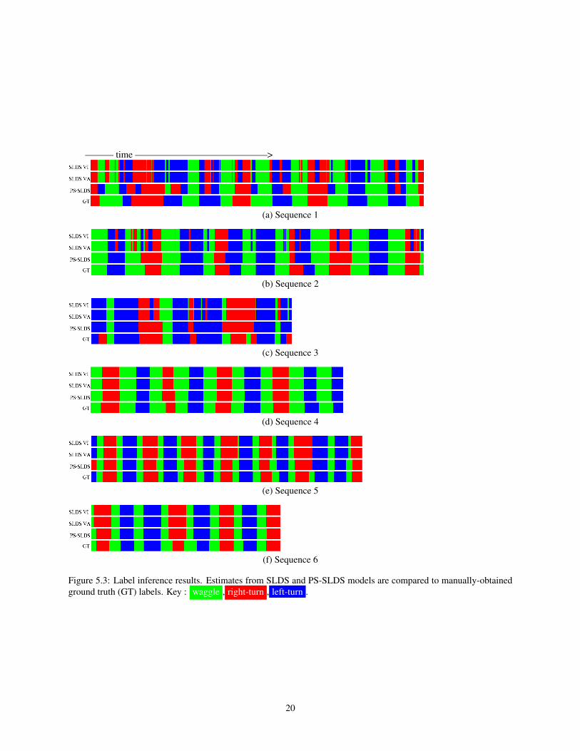
Our experimental results demonstrate the superior recognition capabilities of the proposed PS-SLDS model over theoriginal SLDS model. The label inference results on all data sequences are shown in Fig. 5.3. The four color-codedstrips in each figure represent SLDS VI, SLDS VA, PS-SLDS VI and the ground-truth labels from the top to thebottom. The x-axis represents time flow and the color is the label at that corresponding video frame.

The superior recognition abilities of PS-SLDS can be observed from the presented results. The PS-SLDS resultsare closer to the ground truth or comparable to SLDS results in all sequences. In particular, the sequences 1, 2 and3 are challenging because the tracking results obtained from the vision-based tracker are more noisy. In addition, thepatterns of switching between dance modes and the durations of the dance regime are more irregular than the othersequences.

It can be observed that most of the over-segmentations that appear in the SLDS labeling results disappear in thePS-SLDS labeling results. PS-SLDS estimates still introduce some errors, especially in sequences 1 and 3. However,keeping in mind that even a human expert can introduce labeling noise, the labeling capabilities of PS-SLDS are fairlygood.

5.3.4 Quantitative Results

The quantitative results on the angle/average waggle duration quantification show the robust global parameter quantifi-cation capabilities of PS-SLDS. Table. 5.1 shows (from top to bottom ) : the absolute errors of the PS-SLDS estimatealong with the error rates (%) in parenthesis, SLDS estimates based on the VI and the VA methods, and the groundtruth angle. The best estimates are accented in bold fonts. The SLDS estimates are obtained by the heuristic of aver-aging the heading angles in the sequences that were labeled as “waggle” in the inference step. All of the error valuesare the difference between estimated results and known ground truth values.

Based on the six tests, PS-SLDS and SLDS show comparable waggle angle estimation capabilities. There isno distinguishable gap in performance between VI and VA methods. Our hypothesis is that the over-segmentationerrors do not effect the waggle angle estimate as much as it effects average waggle duration estimates. Note that themaximum error of PS-SLDS angle estimate was 0.11 radians for the fifth dataset, which is fairly good considering thenoise in the tracking results.

The quantitative results on average waggle duration (AWD) quantification show the advantages of PS-SLDS inquantifying the global dynamics parameters of interest. AWD is an indicator of the distance to the food source fromthe hive and is valuable data for insect biologists. Table. 5.2 shows (from top to the bottom) : the absolute errorsand error rates of the PS-SLDS estimates, the SLDS estimates of VI and VA methods and the ground truth AWDs.Again, the best estimates are marked in bold fonts where PS-SLDS estimates are consistently superior to the SLDS

19

——— time ——————————————>

(a) Sequence 1

(b) Sequence 2

(c) Sequence 3

(d) Sequence 4

(e) Sequence 5

(f) Sequence 6

Figure 5.3: Label inference results. Estimates from SLDS and PS-SLDS models are compared to manually-obtainedground truth (GT) labels. Key : waggle , right-turn , left-turn .

20

Sequence 1 2 3 4 5 6PS-SLDS 0.09 (30) 0.01 (4) 0.03 (3) 0.11 (8) 0.11 (5) 0.06 (8)SLDS VI 0.05 (16) 0.03 (12) 0.02 (2) 0.09 (7) 0.18 (9) 0.09 (11)SLDS VA 0.05 (16) 0.03 (12) 0.02 (2) 0.09 (7) 0.18 (9) 0.09 (11)

Ground Truth -0.30 -0.25 1.13 -1.33 -2.08 -0.80

Table 5.1: Absolute errors in the global rotation angle estimates from PS-SLDS and SLDS in radians. The numbersin parenthesis are error rates (%). Last row contains the ground truth rotation angles. Sequence numbers refer to Fig.5.2.

Sequence 1 2 3 4 5 6PS-SLDS 13.7 (27) 0.91 (2) 1.9 (9) 0.22 (<1) 0.4 (2) 5.6 (17)SLDS VI 40.8 (79) 28.9 (62) 11.1 (52) 0.44 (1) 3.6 (19) 8 (25)SLDS VA 40.7 (79) 28.9 (62) 11.1 (52) 0.44 (1) 3.6 (19) 8 (25)

Ground Truth 51.6 46.6 21.4 41.1 19.4 32.6

Table 5.2: Absolute errors in the Average Waggle Duration (AWD) estimates for PS-SLDS and SLDS in frames. Thenumbers in parenthesis are error rates (%). Last row contains the ground truth AWD. Sequence numbers refer to Fig.5.2.

Sequence 1 2 3 4 5 6

PS-SLDS 75.9 92.4 83.1 93.4 90.4 91.0SLDS DD-MCMC 74.0 86.1 81.3 93.4 90.2 90.4

SLDS VI 71.6 82.9 78.9 92.9 89.7 89.2SLDS VA 71.6 82.8 78.9 92.9 89.7 89.2

Table 5.3: Accuracy of label inference in percentage. Sequence numbers refer to Fig. 5.2.

estimates. The SLDS estimates are obtained by evaluating means of the waggle durations in the inferred segments.The results again show that PS-SLDS estimates match the ground-truth closely. In particular, we want to highlight thequality of the PS-SLDS AWD estimates for sequences 2, 3, 4 and 5. In contrast, the SLDS estimates in these casesare inaccurate. More specifically, the SLDS estimates deviate far from the ground truth in most cases except for thesequence 4. The reliability of AWD estimates of PS-SLDS model show the benefit of the duration modeling and thecanonical parameters supported by the enhanced models.

Finally, Table 5.3 shows the overall accuracy of the inferred labels for the PS-SLDS, SLDS DD-MCMC, SLDS VI,and SLDS VA results. It can be observed that PS-SLDS provides very accurate labeling results w.r.t. the ground truth.Moreover, PS-SLDS consistently improves upon the standard SLDSs across all six datasets. The overall experimentalresults show that PS-SLDS model is promising and provides a robust framework for the bee application. It should benoted that SLDS DD-MCMC is the most computationally intensive method, and PS-SLDS still improves on SLDSDD-MCMC in a consistent manner.

5.4 ConclusionIn this section, we presented experimental results on real-world honey bee dance sequences, where the honey beedances were modeled using a parametric segmental SLDS (PS-SLDS) model, i.e. combination of P-SLDS and S-SLDS. Both the qualitative and quantitative results show that the enhanced SLDS model can robustly infer the labelsand global parameters.

A large number of over-segmentations in labeling which appeared in standard SLDSs are not present in the PS-SLDS results. In addition, the results on the quantification abilities of PS-SLDS show that PS-SLDS can provideestimates which are very close to the ground truth . It was also shown that PS-SLDS consistently improves on SLDSsin overall accuracy. The consistent results show that PS-SLDS improves upon SLDS for the honey bee dance data andsuggest that they may be promising for other applications.

21

Chapter 6

Hierarchical SLDS

We propose to develop a hierarchical SLDS (H-SLDS) model as a future work of this proposed research. The H-SLDS model is a generalization of standard SLDSs and is designed to model data with hierarchical structure. Forexample, a hierarchical automaton model that corresponds to the upward-downward triangle sequence in Fig. 6.1(a)is illustrated in Fig. 6.1(b). It can be observed that the shared three primitive dynamic patterns appear in two differenttop substructures with the dependency on the relative position in the sequences. In the flat Markov models, suchrepeating sub-structures (in the middle layer) or primitive dynamic patterns (at the bottom level) need to be redundantlyduplicated under the left-to-right modeling assumption. It is the ability to reuse sub-models in different contexts thatmakes hierarchical models more powerful than flat Markov models.

Good examples of real-world temporal data which exhibit intrinsic hierarchy are honey bees and soccer players,shown in Fig. 6.2. The first example of the honey bee community shown in Fig. 6.2(a) consists of three differenttypes of members, namely a queen, worker bees and drones. While the very primitive motion patterns over short timeduration of all three types of bees would be rather similar, it is the clear difference in longer-term temporal patterns thatlets us to identify the roles of each bee simply from their motion trajectories. For example, a queen bee has relativelyless dynamic motion range over time, while worker bees have the most range of motion such as dancing within thehive and staying on and off from the hive. A potential development of an automated honey bee role classificationsystem might greatly help the field biologists studying the quantitative behavior of bees by saving them a large amountof time needed for hand labeling process. Another example is soccer games, shown in Fig. 6.2(b). A soccer teamconsists of multiple players whose roles differ substantially depending on their positions, i.e., attack middle fielders,defenders, a goal keeper, center forwards, and etc. Again, the motion trajectories of each player over short durationdoes not provide strong cue on their roles. However, the longer-term trajectories provide us with relatively strong clueon the roles of players. Moreover, a player in a fixed position may exhibit multiple different patterns depending onwhether the team is in attack phase or defense phase. Hence, a hierarchical model can be used to identify the top-levelrole of every player as well as the phases the player is transitioning through. In other words, the hierarchical models

(a) (b)

Figure 6.1: (a) An example upward-downward triangle sequence. (b) An example 3-level hierarchical automaton rep-resenting the triangle sequence. Solid lines represent horizontal transitions, dotted lines represent vertical transitions.Double circled nodes represent production states on which the corresponding dynamic patterns are overlaid.

22

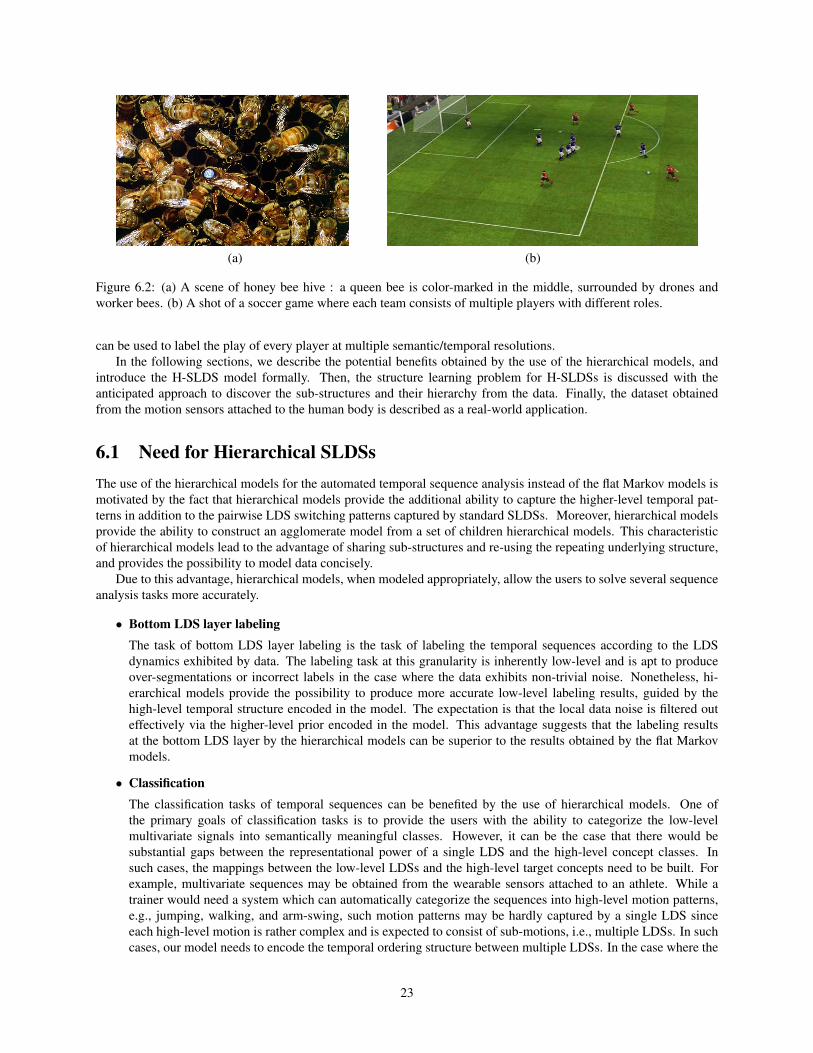
(a) (b)

Figure 6.2: (a) A scene of honey bee hive : a queen bee is color-marked in the middle, surrounded by drones andworker bees. (b) A shot of a soccer game where each team consists of multiple players with different roles.

can be used to label the play of every player at multiple semantic/temporal resolutions.In the following sections, we describe the potential benefits obtained by the use of the hierarchical models, and

introduce the H-SLDS model formally. Then, the structure learning problem for H-SLDSs is discussed with theanticipated approach to discover the sub-structures and their hierarchy from the data. Finally, the dataset obtainedfrom the motion sensors attached to the human body is described as a real-world application.

6.1 Need for Hierarchical SLDSsThe use of the hierarchical models for the automated temporal sequence analysis instead of the flat Markov models ismotivated by the fact that hierarchical models provide the additional ability to capture the higher-level temporal pat-terns in addition to the pairwise LDS switching patterns captured by standard SLDSs. Moreover, hierarchical modelsprovide the ability to construct an agglomerate model from a set of children hierarchical models. This characteristicof hierarchical models lead to the advantage of sharing sub-structures and re-using the repeating underlying structure,and provides the possibility to model data concisely.

Due to this advantage, hierarchical models, when modeled appropriately, allow the users to solve several sequenceanalysis tasks more accurately.

• Bottom LDS layer labelingThe task of bottom LDS layer labeling is the task of labeling the temporal sequences according to the LDSdynamics exhibited by data. The labeling task at this granularity is inherently low-level and is apt to produceover-segmentations or incorrect labels in the case where the data exhibits non-trivial noise. Nonetheless, hi-erarchical models provide the possibility to produce more accurate low-level labeling results, guided by thehigh-level temporal structure encoded in the model. The expectation is that the local data noise is filtered outeffectively via the higher-level prior encoded in the model. This advantage suggests that the labeling resultsat the bottom LDS layer by the hierarchical models can be superior to the results obtained by the flat Markovmodels.

• ClassificationThe classification tasks of temporal sequences can be benefited by the use of hierarchical models. One ofthe primary goals of classification tasks is to provide the users with the ability to categorize the low-levelmultivariate signals into semantically meaningful classes. However, it can be the case that there would besubstantial gaps between the representational power of a single LDS and the high-level concept classes. Insuch cases, the mappings between the low-level LDSs and the high-level target concepts need to be built. Forexample, multivariate sequences may be obtained from the wearable sensors attached to an athlete. While atrainer would need a system which can automatically categorize the sequences into high-level motion patterns,e.g., jumping, walking, and arm-swing, such motion patterns may be hardly captured by a single LDS sinceeach high-level motion is rather complex and is expected to consist of sub-motions, i.e., multiple LDSs. In suchcases, our model needs to encode the temporal ordering structure between multiple LDSs. In the case where the

23

different classes are characterized by the difference in long-term ordering structures, e.g., the example in Fig.6.1, hierarchical models can produce superior classification results by taking the descriptive temporal orderingstructures into account.

• Sharing of sub-structuresAs mentioned above, an important advantage of hierarchical models is that they can share underlying sub-structures. In the case where there are multiple classes of sequences and we are interested in conducting classifi-cation or labeling tasks, the sharing of the sub-structures can boost the re-use of the computation, resulting in thespeed up of inference. Especially, this is advantageous in the case where we are interested in the classificationtasks. The LDS primitives at the bottom level or the short-term repetitive patterns of LDSs in the intermediatelevels can be shared. Moreover, the learning process on multiple classes can discover interesting shared structurefrom data and provide us with more knowledge on the difference between the classes. On the other hand, flatMarkov models have difficulty in structure sharing and does not provide a principled way to combine multiplemodels to a single agglomerate model.

• Labeling with semantically meaningful conceptsThe labeling task with semantically meaningful concepts is to label sequences w.r.t. the high-level semanticsthey exhibit. In fact, this task is equivalent to the sequential classifications task with unknown segment bound-aries. Hierarchical models have recursive structure, i.e., hierarchical models incorporate hierarchical models astheir sub-models at lower layers. Hence, an agglomerate hierarchical model can be built from a set of existingmodels and can be used for the labeling tasks. Such labeling tasks can be hardly conducted by standard SLDSsin principle unless the classes correspond to low-level primitive.

As mentioned above, hierarchical models provide the possibilities to improve on flat Markov models for the sequenceanalysis tasks. There has been previous work on using hierarchical models within with HMMs. The related modelingapproach is hierarchical HMM (H-HMM) [18, 37]. The H-SLDS model to be presented in the following section sharesimilar architecture to H-HHMs in that H-SLDSs adopt hierarchical Markov chain to encode the higher-order structurewithin data. The well-studied formalisms developed for H-HHMs are adopted when necessary with modificationadapted to encode continuous domain that SLDSs address. In the following sections, a definition of hierarchicalSLDSs is introduced and the proposed bottom-up learning approach is discussed.

6.2 Graphical model representation of H-SLDSWe can represent H-SLDS as a dynamic Bayesian network (DBN) as shown in Fig. 6.3(c). The example model hastwo layer hierarchy. The H-SLDS model with additional arcs and finish variables denoted with symbol F is builtincrementally upon the standard SLDS model (shown in Fig. 6.3(a)) through the reasoning steps described in Fig.6.3(a)-(c). In detail, Fig. 6.3(b) shows an SLDS model with a hierarchical Markov chain where the downward arcsfrom the upper layers to the lower layers encode the memberships and state transitions within each regime. Thismodel has been used in previous SLDS extensions [24, 61]. The proposed H-SLDS model in Fig. 6.3(c) has two typesof additional structure : diagonal upward arcs and finish variables. The diagonal upward arcs designed to identifythe lower-level states which trigger the state transitions at the upper levels. And, the finish variable structure helpsthe inference phase to decode the label (segmentation) boundaries more accurately and to enforce the property thattransitions in the upper layers occur only when there is a transition in the lower level. The closest work in terms ofhierarchical Markov chain modeling would be the H-HMM work by Murphy and Paskin [37].

More in detail, each discrete node is denoted as l(h)t with the superscript (h) corresponding to the height of the

layer where the bottom level corresponds to the layer level 1 and increases upward. The subscript t denotes thecorresponding time-step. A slice of the DBN is marked in the dashed rectangle in Fig. 6.3. The state of the wholeH-SLDS at time t is represented by the discrete state vector L1:N

t∆= [l1t , l

2t , ..., l

Nt ] where the height of the hierarchy is

N , and the continuous state xt with the corresponding observation zt.The finish variable f

(h)t at the h-th layer is a Boolean variable which indicates that the current regime conditioned

by the ancestor variables L(h+1):Nt finishes at time t when f

(h)t = true. In the case where f

(h)t = false , the current

regime at the h- layer continues with the the ancestor variables remaining constant, i.e., L(h+1):Nt ← L

(h+1):Nt−1 . Note

that if f(h)t = true, then for all the levels below h′ < h, the finish variables are true, i.e., f (h′)

t = true. The downward

24

(a) (b)

(c)

Figure 6.3: Graphical model representations of the hierarchical SLDS models. Note that the model of interestin this proposal is (c). The series of figures demonstrate the role of new structure one by one. (a) A graphicalmodel of standard SLDSs. (b) Hierarchical Markov chain in the green boxed rectangle extends the conventional flatMarkov chain in the standard SLDS model. The downward arcs from the upper layers to the lower layers encode thememberships and state transitions within each regime. (c) Proposed H-SLDS model. Additional structure of finishvariables and diagonal upward arcs are introduced to descriptively indicate the lower-level states which trigger thestate transitions at the upper level. The newly introduced finish variable structure allows the inference phase to decodethe segmentation boundaries more accurately and to enforce the property that transitions in the upper layers occur onlywhen there is a transition in the lower level.

25

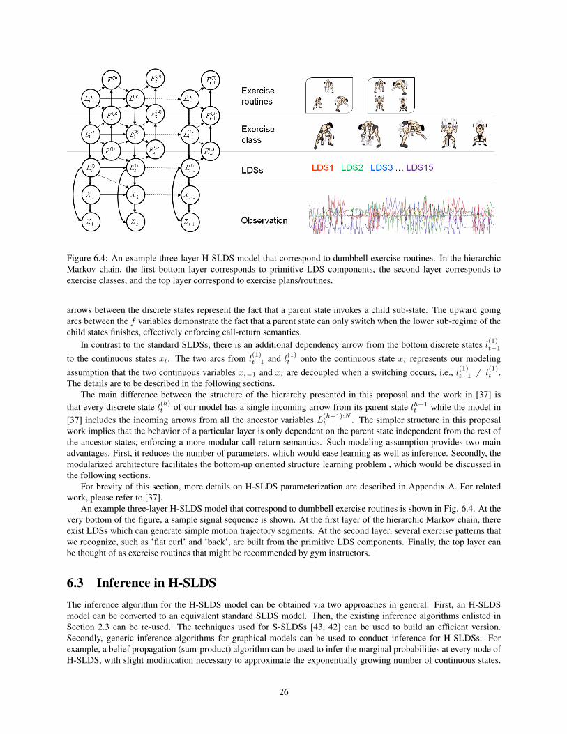
Figure 6.4: An example three-layer H-SLDS model that correspond to dumbbell exercise routines. In the hierarchicMarkov chain, the first bottom layer corresponds to primitive LDS components, the second layer corresponds toexercise classes, and the top layer correspond to exercise plans/routines.

arrows between the discrete states represent the fact that a parent state invokes a child sub-state. The upward goingarcs between the f variables demonstrate the fact that a parent state can only switch when the lower sub-regime of thechild states finishes, effectively enforcing call-return semantics.

In contrast to the standard SLDSs, there is an additional dependency arrow from the bottom discrete states l(1)t−1

to the continuous states xt. The two arcs from l(1)t−1 and l

(1)t onto the continuous state xt represents our modeling

assumption that the two continuous variables xt−1 and xt are decoupled when a switching occurs, i.e., l(1)t−1 6= l

(1)t .

The details are to be described in the following sections.The main difference between the structure of the hierarchy presented in this proposal and the work in [37] is

that every discrete state l(h)t of our model has a single incoming arrow from its parent state lh+1

t while the model in[37] includes the incoming arrows from all the ancestor variables L

(h+1):Nt . The simpler structure in this proposal

work implies that the behavior of a particular layer is only dependent on the parent state independent from the rest ofthe ancestor states, enforcing a more modular call-return semantics. Such modeling assumption provides two mainadvantages. First, it reduces the number of parameters, which would ease learning as well as inference. Secondly, themodularized architecture facilitates the bottom-up oriented structure learning problem , which would be discussed inthe following sections.

For brevity of this section, more details on H-SLDS parameterization are described in Appendix A. For relatedwork, please refer to [37].

An example three-layer H-SLDS model that correspond to dumbbell exercise routines is shown in Fig. 6.4. At thevery bottom of the figure, a sample signal sequence is shown. At the first layer of the hierarchic Markov chain, thereexist LDSs which can generate simple motion trajectory segments. At the second layer, several exercise patterns thatwe recognize, such as ’flat curl’ and ’back’, are built from the primitive LDS components. Finally, the top layer canbe thought of as exercise routines that might be recommended by gym instructors.

6.3 Inference in H-SLDSThe inference algorithm for the H-SLDS model can be obtained via two approaches in general. First, an H-SLDSmodel can be converted to an equivalent standard SLDS model. Then, the existing inference algorithms enlisted inSection 2.3 can be re-used. The techniques used for S-SLDSs [43, 42] can be used to build an efficient version.Secondly, generic inference algorithms for graphical-models can be used to conduct inference for H-SLDSs. Forexample, a belief propagation (sum-product) algorithm can be used to infer the marginal probabilities at every node ofH-SLDS, with slight modification necessary to approximate the exponentially growing number of continuous states.

26

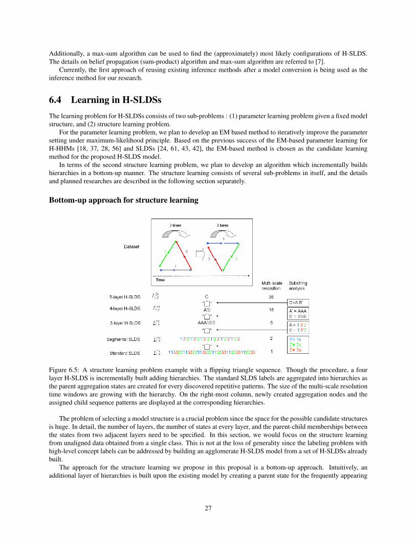
Additionally, a max-sum algorithm can be used to find the (approximately) most likely configurations of H-SLDS.The details on belief propagation (sum-product) algorithm and max-sum algorithm are referred to [7].

Currently, the first approach of reusing existing inference methods after a model conversion is being used as theinference method for our research.

6.4 Learning in H-SLDSsThe learning problem for H-SLDSs consists of two sub-problems : (1) parameter learning problem given a fixed modelstructure, and (2) structure learning problem.

For the parameter learning problem, we plan to develop an EM based method to iteratively improve the parametersetting under maximum-likelihood principle. Based on the previous success of the EM-based parameter learning forH-HHMs [18, 37, 28, 56] and SLDSs [24, 61, 43, 42], the EM-based method is chosen as the candidate learningmethod for the proposed H-SLDS model.

In terms of the second structure learning problem, we plan to develop an algorithm which incrementally buildshierarchies in a bottom-up manner. The structure learning consists of several sub-problems in itself, and the detailsand planned researches are described in the following section separately.

Bottom-up approach for structure learning

Figure 6.5: A structure learning problem example with a flipping triangle sequence. Though the procedure, a fourlayer H-SLDS is incrementally built adding hierarchies. The standard SLDS labels are aggregated into hierarchies asthe parent aggregation states are created for every discovered repetitive patterns. The size of the multi-scale resolutiontime windows are growing with the hierarchy. On the right-most column, newly created aggregation nodes and theassigned child sequence patterns are displayed at the corresponding hierarchies.

The problem of selecting a model structure is a crucial problem since the space for the possible candidate structuresis huge. In detail, the number of layers, the number of states at every layer, and the parent-child memberships betweenthe states from two adjacent layers need to be specified. In this section, we would focus on the structure learningfrom unaligned data obtained from a single class. This is not at the loss of generality since the labeling problem withhigh-level concept labels can be addressed by building an agglomerate H-SLDS model from a set of H-SLDSs alreadybuilt.

The approach for the structure learning we propose in this proposal is a bottom-up approach. Intuitively, anadditional layer of hierarchies is built upon the existing model by creating a parent state for the frequently appearing

27

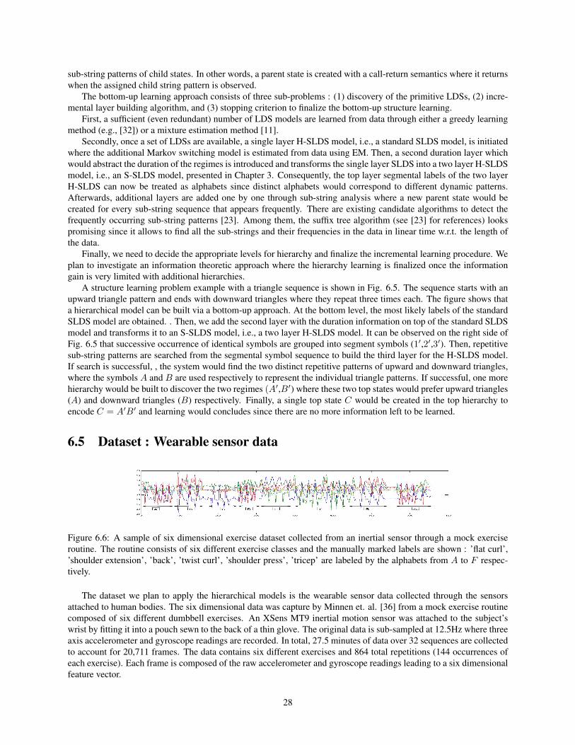
sub-string patterns of child states. In other words, a parent state is created with a call-return semantics where it returnswhen the assigned child string pattern is observed.

The bottom-up learning approach consists of three sub-problems : (1) discovery of the primitive LDSs, (2) incre-mental layer building algorithm, and (3) stopping criterion to finalize the bottom-up structure learning.

First, a sufficient (even redundant) number of LDS models are learned from data through either a greedy learningmethod (e.g., [32]) or a mixture estimation method [11].

Secondly, once a set of LDSs are available, a single layer H-SLDS model, i.e., a standard SLDS model, is initiatedwhere the additional Markov switching model is estimated from data using EM. Then, a second duration layer whichwould abstract the duration of the regimes is introduced and transforms the single layer SLDS into a two layer H-SLDSmodel, i.e., an S-SLDS model, presented in Chapter 3. Consequently, the top layer segmental labels of the two layerH-SLDS can now be treated as alphabets since distinct alphabets would correspond to different dynamic patterns.Afterwards, additional layers are added one by one through sub-string analysis where a new parent state would becreated for every sub-string sequence that appears frequently. There are existing candidate algorithms to detect thefrequently occurring sub-string patterns [23]. Among them, the suffix tree algorithm (see [23] for references) lookspromising since it allows to find all the sub-strings and their frequencies in the data in linear time w.r.t. the length ofthe data.

Finally, we need to decide the appropriate levels for hierarchy and finalize the incremental learning procedure. Weplan to investigate an information theoretic approach where the hierarchy learning is finalized once the informationgain is very limited with additional hierarchies.

A structure learning problem example with a triangle sequence is shown in Fig. 6.5. The sequence starts with anupward triangle pattern and ends with downward triangles where they repeat three times each. The figure shows thata hierarchical model can be built via a bottom-up approach. At the bottom level, the most likely labels of the standardSLDS model are obtained. . Then, we add the second layer with the duration information on top of the standard SLDSmodel and transforms it to an S-SLDS model, i.e., a two layer H-SLDS model. It can be observed on the right side ofFig. 6.5 that successive occurrence of identical symbols are grouped into segment symbols (1′,2′,3′). Then, repetitivesub-string patterns are searched from the segmental symbol sequence to build the third layer for the H-SLDS model.If search is successful, , the system would find the two distinct repetitive patterns of upward and downward triangles,where the symbols A and B are used respectively to represent the individual triangle patterns. If successful, one morehierarchy would be built to discover the two regimes (A′,B′) where these two top states would prefer upward triangles(A) and downward triangles (B) respectively. Finally, a single top state C would be created in the top hierarchy toencode C = A′B′ and learning would concludes since there are no more information left to be learned.

6.5 Dataset : Wearable sensor data

Figure 6.6: A sample of six dimensional exercise dataset collected from an inertial sensor through a mock exerciseroutine. The routine consists of six different exercise classes and the manually marked labels are shown : ’flat curl’,’shoulder extension’, ’back’, ’twist curl’, ’shoulder press’, ’tricep’ are labeled by the alphabets from A to F respec-tively.

The dataset we plan to apply the hierarchical models is the wearable sensor data collected through the sensorsattached to human bodies. The six dimensional data was capture by Minnen et. al. [36] from a mock exercise routinecomposed of six different dumbbell exercises. An XSens MT9 inertial motion sensor was attached to the subject’swrist by fitting it into a pouch sewn to the back of a thin glove. The original data is sub-sampled at 12.5Hz where threeaxis accelerometer and gyroscope readings are recorded. In total, 27.5 minutes of data over 32 sequences are collectedto account for 20,711 frames. The data contains six different exercises and 864 total repetitions (144 occurrences ofeach exercise). Each frame is composed of the raw accelerometer and gyroscope readings leading to a six dimensionalfeature vector.

28

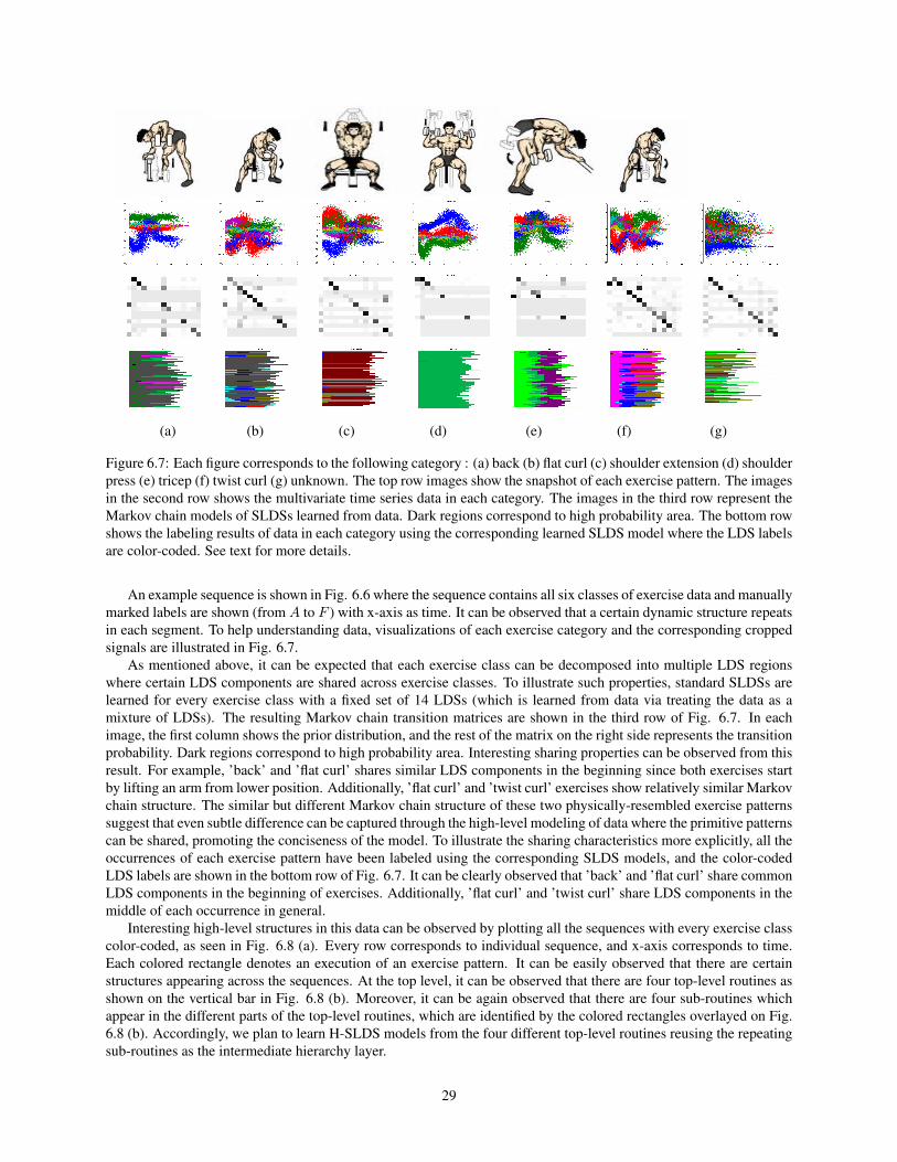
(a) (b) (c) (d) (e) (f) (g)

Figure 6.7: Each figure corresponds to the following category : (a) back (b) flat curl (c) shoulder extension (d) shoulderpress (e) tricep (f) twist curl (g) unknown. The top row images show the snapshot of each exercise pattern. The imagesin the second row shows the multivariate time series data in each category. The images in the third row represent theMarkov chain models of SLDSs learned from data. Dark regions correspond to high probability area. The bottom rowshows the labeling results of data in each category using the corresponding learned SLDS model where the LDS labelsare color-coded. See text for more details.

An example sequence is shown in Fig. 6.6 where the sequence contains all six classes of exercise data and manuallymarked labels are shown (from A to F ) with x-axis as time. It can be observed that a certain dynamic structure repeatsin each segment. To help understanding data, visualizations of each exercise category and the corresponding croppedsignals are illustrated in Fig. 6.7.

As mentioned above, it can be expected that each exercise class can be decomposed into multiple LDS regionswhere certain LDS components are shared across exercise classes. To illustrate such properties, standard SLDSs arelearned for every exercise class with a fixed set of 14 LDSs (which is learned from data via treating the data as amixture of LDSs). The resulting Markov chain transition matrices are shown in the third row of Fig. 6.7. In eachimage, the first column shows the prior distribution, and the rest of the matrix on the right side represents the transitionprobability. Dark regions correspond to high probability area. Interesting sharing properties can be observed from thisresult. For example, ’back’ and ’flat curl’ shares similar LDS components in the beginning since both exercises startby lifting an arm from lower position. Additionally, ’flat curl’ and ’twist curl’ exercises show relatively similar Markovchain structure. The similar but different Markov chain structure of these two physically-resembled exercise patternssuggest that even subtle difference can be captured through the high-level modeling of data where the primitive patternscan be shared, promoting the conciseness of the model. To illustrate the sharing characteristics more explicitly, all theoccurrences of each exercise pattern have been labeled using the corresponding SLDS models, and the color-codedLDS labels are shown in the bottom row of Fig. 6.7. It can be clearly observed that ’back’ and ’flat curl’ share commonLDS components in the beginning of exercises. Additionally, ’flat curl’ and ’twist curl’ share LDS components in themiddle of each occurrence in general.

Interesting high-level structures in this data can be observed by plotting all the sequences with every exercise classcolor-coded, as seen in Fig. 6.8 (a). Every row corresponds to individual sequence, and x-axis corresponds to time.Each colored rectangle denotes an execution of an exercise pattern. It can be easily observed that there are certainstructures appearing across the sequences. At the top level, it can be observed that there are four top-level routines asshown on the vertical bar in Fig. 6.8 (b). Moreover, it can be again observed that there are four sub-routines whichappear in the different parts of the top-level routines, which are identified by the colored rectangles overlayed on Fig.6.8 (b). Accordingly, we plan to learn H-SLDS models from the four different top-level routines reusing the repeatingsub-routines as the intermediate hierarchy layer.

29

(a) (b)

Figure 6.8: (a) Color plotting of exercises occurring across data sequences. Each row corresponds to different se-quence, and colored rectangles denote executions of the corresponding exercises. (b) Four different top-level routinesare marked on the left vertical bar, and four different sub-routines are overlayed by colored rectangles.

With the learned H-SLDS models, we plan to analyze the learned structure to examine whether H-SLDSs canlearn meaningful structure from data. Additionally, we plan to conduct classification and labeling tasks based on thelearned models to distinguish sequences from different routines and provide automatic exercise annotation at multiplegranularity. The results would provide measures to examine the hierarchical analysis power of the proposed H-SLDSmodel. Standard SLDSs would be used as the baseline model when appropriate, e.g., classification tasks.

6.6 Summary : Planned Future WorkIn summary, we plan to address the following remaining issues for H-SLDSs :

• Development of an EM-based parameter learning algorithm

• Development of a bottom-up learning algorithm which can learn hierarchic model structure from data

• Test of the developed methods on the real-world wearable sensor data for labeling and classification tasks.

6.7 Related WorkHMMs are by far the most studied model for the temporal sequence analysis. The study on the hierarchical aspectof SLDSs in this proposal is also partly inspired by the previous work on H-HMMs. We review the related work onHMMs first, then describe the previous work on hierarchical models with continuous dynamics.

6.7.1 Hierarchical HMMsThe most closely related modeling work to H-SLDS in HMM community is hierarchical HMMs (H-HMMs). H-HMMs have been introduced by Fine et al.[18] where the hierarchical structure was developed to capture the long-termcorrelations between the elementary observations. For example, Fine et al.[18] applied H-HMMs for the problemsof English text modeling and cursive hand-writing recognition where they hand-crafted the model and learned theparameters from the data. Murphy and Paskin [37] introduced a DBN representation for H-HMMs and a linear timeO(T ) inference algorithm for H-HMMs, w.r.t. the length of the observation T . The graphical model representation ofH-SLDS in Fig. 6.2 follows their DBN representation.

H-HMMs have been used for video analysis for play/break labeling for soccer videos [28] and two-layer H-HMMshave been used for the video-based activity recognition within home environments [56].

30

6.7.2 Hierarchical Models with Continuous DynamicsWe review previous work on the SLDS models with hierarchies. A work by Howard by Jebera, ’Dynamical SystemTrees’ (DSTs) [24], has a tree structure where the leaves of a tree correspond to an individual agent and the whole treerepresents group behaviors. A branch of DST from the top node to a leaf node is analogous to the model shown in Fig.6.3(b). DSTs have been used to classify attack/defense modes of American football video. While their work providesa novel inference algorithm based on structured variational methods, the structures of the models are hand-crafted bythe users and the best model is selected through trials.

Another closely related work is ’Multi-scale SLDSs’ (MS-SLDS) by Zoeter and Heskes [61]. The MS-SLDSmodel has a graphical model similar to is analogous to the model shown in Fig. 6.3(b). Hence, the parent state canswitch at anytime and does not have the call-return semantics of the H-SLDS model. They introduce an inferencealgorithm based on Expectation Propagation [35] method, but does not address the structure learning issues.

The segmental SLDS (S-SLDS) model [43, 42] presented in Chapter 3 of this proposal is a special case of H-SLDSs. S-SLDS is a two layer model where the top layer switches between regimes and the bottom layer counts thedurations.

31

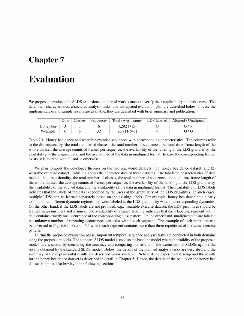
Chapter 7

Evaluation

We propose to evaluate the SLDS extensions on the real world dataset to verify their applicability and robustness. Thedata, their characteristics, associated analysis tasks, and anticipated evaluation plan are described below. In case theimplementation and sample results are available, they are described with brief summary and publication.

Dim Classes Sequences Total (Avg) frames LDS labeled Aligned / UnalignedHoney bee 3 3 6 4,292 (715) O O / ×Wearable 6 6 32 20,711(647) × O / O

Table 7.1: Honey bee dance and wearable exercise sequences with corresponding characteristics. The columns referto the dimensionality, the total number of classes, the total number of sequences, the total time frame length of thewhole dataset, the average counts of frames per sequence, the availability of the labeling at the LDS granularity, theavailability of the aligned data, and the availability of the data in unaligned format. In case the corresponding formatexists, it is marked with O, and × otherwise.

We plan to apply the developed theories on the two real world datasets : (1) honey bee dance dataset, and (2)wearable exercise dataset. Table 7.1 shows the characteristics of these datasets. The tabulated characteristics of datainclude the dimensionality, the total number of classes, the total number of sequences, the total time frame length ofthe whole dataset, the average counts of frames per sequence, the availability of the labeling at the LDS granularity,the availability of the aligned data, and the availability of the data in unaligned format. The availability of LDS labelsindicates that the labels of the data is specified by the users at the granularity of the LDS primitives. In such cases,multiple LDSs can be learned separately based on the existing labels. For example, honey bee dance data clearlyexhibits three different dynamic regimes and were labeled at the LDS granularity w.r.t. the corresponding dynamics.On the other hand, if the LDS labels are not provided, e.g., wearable exercise dataset, the LDS primitives should belearned in an unsupervised manner. The availability of aligned labeling indicates that each labeling segment withindata contains exactly one occurrence of the corresponding class pattern. On the other hand, unaligned data are labeledbut unknown number of repeating occurrences can exist within each segment. The example of such repetition canbe observed in Fig. 6.6 in Section 6.5 where each segment contains more than three repetitions of the same exercisepattern.

During the proposed evaluation phase, important temporal sequence analysis tasks are conducted in both domainsusing the proposed models. The standard SLDS model is used as the baseline model where the validity of the proposedmodels are assessed by measuring the accuracy and comparing the results of the extensions of SLDSs against theresults obtained by the standard SLDS model. Below, the details of the planned analysis tasks are described and thesummary of the experimental results are described when available. Note that the experimental setup and the resultsfor the honey bee dance dataset is described in detail in Chapter 5. Hence, the details of the results on the honey beedataset is omitted for brevity in the following sections.

32

S-SLDS P-SLDS PS-SLDS H-SLDS

Honey bee dance dataset

Superior labeling[43]

in Chapter 3

Superior globalvariable

quantification [41]in Chapter 4

Superior labelingand quantification

[43, 42]in Chapter 5

Wearable exercise dataset

A part of H-SLDSwork

In Chapter 6October 2008

Table 7.2:Evaluation grid showing the various extensions of SLDSs against the two datasets. Citations, corresponding chaptersand summary of evaluation results are provided for already implemented cases while an expected completion date isprovided in other cases.

7.1 Honey bee dance dataset• Labeling

Standard SLDS (Chapter 2) and PS-SLDS (Chapter 3, 4) models are learned from data where the availablelabels are used to conduct supervised learning. Then, the accuracy of the labeling results obtained from PS-SLDSs are compared w.r.t. the existing ground-truth labels to verify the benefits of the additional duration andglobal parameter modeling in the PS-SLDS model. The experimental results showed that the learned PS-SLDSssubstantially and consistently outperform standard SLDSs [41, 43, 42].

• Global parameter quantificationA PS-SLDS (Chapter 3, 4, 4) model is learned from data where the labels and the known global parameters, e.g.,angle and duration of the dances, are used to learn the canonical template of honey bee dances and the globalparameterization. The learned model was used to find the angles and the durations of the honey bee danceswhere the labeling and the quantization tasks were conducted simultaneously. Another set of global parameterestimates were obtained using standard SLDSs through a post-processing step which is designed to estimate theglobal parameters from the SLDS labels. Then, the accuracy of quantified global parameters and the obtainedlabels are compared to the available ground truth values. The experimental results demonstrated that the globalparameters and the labels obtained by PS-SLDSs are consistently superior to those of SLDSs both qualitativelyand quantitatively [41, 42].

7.2 Wearable exercise datasetAs proposed in Chapter 6, we plan to develop a structure learning algorithm for H-SLDSs and apply it to the wearableexercise dataset. The plan is to assess the benefits of the H-SLDS model over the standard SLDSs on the wearableexercise dataset described in Section. 6.5. Both the H-SLDS model and the standard SLDS models are to be learnedfrom the routine and out-of-routine dataset.

• ClassificationThe learned H-SLDS and standard SLDS models are to be tested for classification tasks where both the routineand out-of-routine data are planned to be used as test dataset.

• LabelingOnce H-SLDSs and SLDSs are learned for the classification tasks, they can be used for labeling. In principle,H-SLDSs provide a natural way to combine the learned sub-models into a single agglomerate model which

33

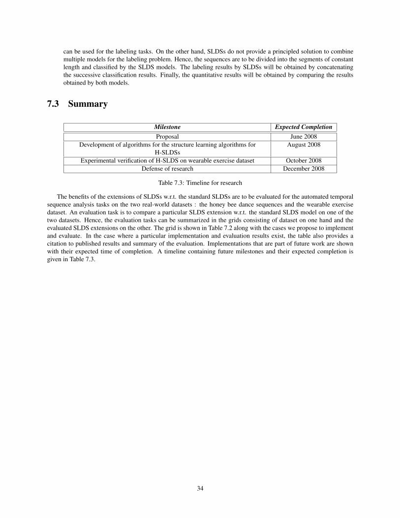
can be used for the labeling tasks. On the other hand, SLDSs do not provide a principled solution to combinemultiple models for the labeling problem. Hence, the sequences are to be divided into the segments of constantlength and classified by the SLDS models. The labeling results by SLDSs will be obtained by concatenatingthe successive classification results. Finally, the quantitative results will be obtained by comparing the resultsobtained by both models.

7.3 Summary

Milestone Expected CompletionProposal June 2008

Development of algorithms for the structure learning algorithms forH-SLDSs

August 2008

Experimental verification of H-SLDS on wearable exercise dataset October 2008Defense of research December 2008

Table 7.3: Timeline for research

The benefits of the extensions of SLDSs w.r.t. the standard SLDSs are to be evaluated for the automated temporalsequence analysis tasks on the two real-world datasets : the honey bee dance sequences and the wearable exercisedataset. An evaluation task is to compare a particular SLDS extension w.r.t. the standard SLDS model on one of thetwo datasets. Hence, the evaluation tasks can be summarized in the grids consisting of dataset on one hand and theevaluated SLDS extensions on the other. The grid is shown in Table 7.2 along with the cases we propose to implementand evaluate. In the case where a particular implementation and evaluation results exist, the table also provides acitation to published results and summary of the evaluation. Implementations that are part of future work are shownwith their expected time of completion. A timeline containing future milestones and their expected completion isgiven in Table 7.3.

34

Chapter 8

Summary of Contribution

The following are the major contributions of the work proposed and described here -

1. The principled formulations of the SLDS extensions in the popular graphical model framework and the devel-opment of the associated learning and inference algorithms.

• S-SLDSs encode the duration patterns within each regime. A systematic approach to re-use an array ofpre-existing inference algorithms for the standard SLDS models for S-SLDSs are introduced.

• P-SLDSs explicitly encodes the global parameters which cause systematic variations within data. Learningand inference algorithms based on EM are introduced accordingly.

• H-SLDSs encode descriptive temporal structure in hierarchies to capture both repetitive sub-structures andlong-term correlations. We propose to study both inference and learning algorithms for H-SLDSs.

2. Instantiations of the above theory for various automated temporal sequence analysis tasks and their applicationon the honey bee dance dataset and results thereof

To validate our claim on the benefits of modeling the higher-level knowledge over the standard flat SLDSs, weapply S-SLDSs, P-SLDSs and PS-SLDSs to the honey bee dance dataset. The extensions of SLDSs produceconsistently more accurate results for the labeling and global parameter quantification tasks.

3. Evaluation of the H-SLDS model framework on the wearable exercise dataset

We plan to evaluate the H-SLDS model for the wearable exercise dataset in the absence of manual LDS labels.We plan to learn the H-SLDS model from the data in automatic manner. The evaluation results are conjecturedto deliver an empirical evidence on the benefits of hierarchical models for the datasets with unknown complextemporal structures.

In addition, we envision that the formulation of the SLDS extensions in the popular graphical model framework,the availability of the associated learning and inference algorithms, and experimentally validated usefulness of theproposed models will promote the use of the switching models with continuous dynamics for the temporal sequenceanalysis tasks.

35

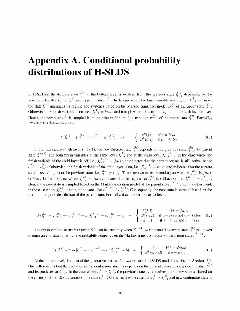
Appendix A. Conditional probabilitydistributions of H-SLDS

In H-SLDSs, the discrete state l(1)t at the bottom layer is evolved from the previous state l

(1)t−1 depending on the

associated finish variable f(1)t−1 and its parent state l

(2)t . In the case where the finish variable was off, i.e., f (1)

t−1 = false,

the state l(h)t maintains its regime and switches based on the Markov transition model Bl

(2)t of the upper state l

(2)t .

Otherwise, the finish variable is on, i.e., f(1)t−1 = true, and it implies that the current regime on the h-th layer is over.

Hence, the new state l(1)t is sampled from the prior multinomial distribution πL

(2)t of the parent state l

(2)t . Formally,

we can write this as follows :

P (l(1)t = j|l(1)t−1 = i, l(2)t = k, f

(1)t−1 = v) =

{πk(j) if v = true

Bk(i, j) if v = false(8.1)

In the intermediate h-th layer (h > 1), the new discrete state l(h)t depends on the previous state l

(h)t−1, the parent

state l(h+1)t , and both finish variables at the same level f

(h)t−1 and at the child level f

(h−1)t−1 . In the case where the

finish variable of the child layer is off, i.e., f(h−1)t−1 = false, it indicates that the current regime is still active, hence

l(h)t ← l

(h)t−1. Otherwise, the finish variable of the child layer is on, i.e., f

(h−1)t−1 = true, and indicates that the current

state is switching from the previous state, i.e., l(h)t 6= l

(h)t−1. There are two cases depending on whether f

(h)t−1 is false

or true. In the first case where f(h)t−1 = false, it states that the regime for l

(h)t−1 is still active, i.e., l

(h+1)t = l

(h+1)t−1 .

Hence, the new state is sampled based on the Markov transition model of the parent state l(h+1)t . On the other hand,

in the case where f(h)t−1 = true, it indicates that l

(h+1)t 6= l

(h+1)t−1 . Consequently, the new state is sampled based on the

multinomial prior distribution of the parent state. Formally, it can be written as follows :

P (l(h)t = j|l(h)

t−1 = i, l(h+1)t = k, f

(h−1)t−1 = b, f

(h)t−1 = v) =

δ(j, i) if b = false

Bk(i, j) if b = true and v = falseπk(j) if b = true and v = true

(8.2)

The finish variable at the h-th layer f(h)t can be true only when f

(h−1)t = true and the current state l

(h)t is allowed

to enter an end state, of which the probability depends on the Markov transition model of the parent state l(h+1)t :

P (f (h)t = true|l(h)

t = i, l(h+1)t = k, f

(h−1)t−1 = b) =

{0 if b = false

Bk(i, end) if b = true(8.3)

At the bottom level, the most of the generative process follows the standard SLDS model described in Section. 2.2.One difference is that the evolution of the continuous state xt depends on the current corresponding discrete state l

(1)t

and its predecessor l(1)t−1. In the case where l

(1)t = l

(1)t−1, the previous state xt−1 evolves into a new state xt based on

the corresponding LDS dynamics of the state l(1)t . Otherwise, it is the case that l

(1)t 6= l

(1)t−1 and new continuous state is

36

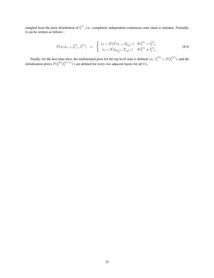
sampled from the prior distribution of l(1)t , i.e., completely independent continuous state chain is initiated. Formally,

it can be written as follows :

P (xt|xt−1, l(1)t−1, l

(1)t ) =

{xt ∼ N (Fxt−1, QL

(1)t

) if l(1)t = l

(1)t−1

xt ∼ N (µL

(1)t

,ΣL

(1)t

) if l(1)t 6= l

(1)t−1

(8.4)

Finally, for the first time-slice, the multinomial prior for the top level state is defined, i.e., l(N)1 ∼ P (l(N)

1 ), and theinitialization priors P (l(h)

1 |l(h+1)1 )’s are defined for every two adjacent layers for all h’s.

37

Bibliography

[1] Proc. 17th Conf. on Uncertainty in AI (UAI), Seattle, WA, August 2001.

[2] T. Balch, F. Dellaert, A. Feldman, A. Guillory, C. Isbell, Z. Khan, A. Stein, and H. Wilde. How A.I. andmulti-robot systems research will accelerate our understanding of social animal behavior. Proceedings of IEEE,94(7):1145–1463, July 2006.

[3] T. Balch, Z. Khan, and M. Veloso. Automatically tracking and analyzing the behavior of live insect colonies. InProc. Autonomous Agents 2001, pages 521–528, Montreal, 2001.

[4] Y. Bar-Shalom and X. Li. Estimation and Tracking: principles, techniques and software. Artech House, Boston,London, 1993.

[5] Y. Bar-Shalom and E. Tse. Tracking in a cluttered environment with probabilistic data-association. Automatica,11:451–460, 1975.

[6] D. J. Bartholomew. Latent Variable Models and Factor Analysis. Oxford University Press, New York, 1987.

[7] Christopher M. Bishop. Pattern Recognition and Machine Learning. Springer, 2007.

[8] K. Branson and S. Belongie. Tracking multiple mouse contours (without too many samples). In IEEE Conf. onComputer Vision and Pattern Recognition (CVPR), volume 1, pages 1039–1046, 2005.

[9] C. Bregler. Learning and Recognizing Human Dynamics in Video Sequences. In IEEE Conf. on Computer Visionand Pattern Recognition (CVPR), pages 568–574, 1997.

[10] C. Carter and R. Kohn. Markov chain Monte Carlo in Conditionally Gaussian State Spaece Models. Biometrika,83:589–601, 1996.

[11] A. B. Chan and N. Vasconcelos. Mixtures of Dynamic Textures. In Intl. Conf. on Computer Vision (ICCV), 2005.

[12] A.P. Dempster, N.M. Laird, and D.B. Rubin. Maximum likelihood from incomplete data via the EM algorithm.Journal of the Royal Statistical Society, Series B, 39(1):1–38, 1977.

[13] P. M. Djuric and J-H. Chun. An MCMC Sampling Approach to Estimation of Nonstationary Hidden MarkovModels. IEEE Trans. Signal Processing, 50(5):1113–1123, 2002.

[14] G. Doretto, A. Chiuso, Y. Wu, and S. Soatto. Dynamic Textures. Intl. J. of Computer Vision, 51(2):91–109, 2003.

[15] A. Doucet and C. Andrieu. Iterative Algorithms for State Estimation of Jump Markov Linear Systems. IEEETrans. Signal Processing, 49(6):1216–1227, 2001.

[16] A. Doucet, N. J. Gordon, and V. Krishnamurthy. Particle filters for state estimation of jump Markov linearsystems. IEEE Trans. Signal Processing, 49(3):613–624, 2001.

[17] J. Ferguson. Variable duration models for speech. In Symposium on the Aplication of HMMs to Text and Speech,pages 143–179, 1980.

[18] S. Fine, Y. Singer, and N. Tishby. The Hierarchical Hidden Markov Model : Analysis and Applications. Machinelearning, 32:41–62, 1998.

38

[19] K. Frisch. The Dance Language and Orientation of Bees. Harvard University Press, 1967.

[20] X. Ge and P. Smyth. Deformable Markov model templates for time-series pattern matching. In Intl. Conf.Knowledge Discovery and Data Mining (KDD), pages 81–90, 2000.

[21] Z. Ghahramani and G. E. Hinton. Variational learning for switching state-space models. Neural Computation,12(4):963–996, 1998.

[22] Z. Ghahramani and G.E. Hinton. The EM algorithm for mixtures of factor analyzers. Technical Report CRG-TR-96-1, Dept. of Computer Science, University of Toronto, February 1997.

[23] Dan Gusfield. Algorithms on Strings, Trees and Sequences: Computer Science and Computational Biology.Cambridge University Press, 1997.

[24] A. Howard and T. Jebara. Dynamical systems trees. In Proc. 20th Conf. on Uncertainty in AI (UAI), pages260–267, Banff, Canada, July 2004.

[25] Z. Khan, T. Balch, and F. Dellaert. A Rao-Blackwellized particle filter for EigenTracking. In IEEE Conf. onComputer Vision and Pattern Recognition (CVPR), volume 2, pages 980–986, 2004.

[26] C.-J. Kim. Dynamic linear models with Markov-switching. Journal of Econometrics, 60(1-2):1–22, 1994.

[27] S. Kim and P. Smyth. Segmental Hidden Markov Models with Random Effects for Waveform Modeling. J. ofMachine Learning Research, 7:945–969, October 2006.

[28] A. Divakaran L. Xie, S.-F. Chang and H. Sun. Unsupervised Discovery of Multilevel Statistical Video StructuresUsing Hierarchical Hidden Markov Models. In IEEE Intl. Conf. on Multimedia and Expo(ICME), volume 3,pages 29–32, 2003.

[29] U. Lerner and R. Parr. Inference in hybrid networks: Theoretical limits and practical algorithms. In Proc. 17th

Conf. on Uncertainty in AI (UAI) [1], pages 310–318.

[30] U. Lerner, R. Parr, D. Koller, and G. Biswas. Bayesian fault detection and diagnosis in dynamic systems. InProc. 17th AAAI National Conference on AI, pages 531–537, Austin, TX, 2000.

[31] S. E. Levinson. Continuously variable duration hidden Markov models for automatic speech recognition. Com-puter Speech and Language, 1(1):29–45, 1990.

[32] Y. Li and T. Wang ad H-Y. Shum. Motion texture : A two-level statistical model for character motion synthesis.In SIGGRAPH, 2002.

[33] P. Maybeck. Stochastic Models, Estimation and Control, volume 1. Academic Press, New York, 1979.

[34] G.J. McLachlan and T. Krishnan. The EM algorithm and extensions. Wiley series in probability and statistics.John Wiley & Sons, 1997.

[35] Thomas P. Minka. Expectation propagation for approximate Bayesian inference. In Proc. 17th Conf. on Uncer-tainty in AI (UAI) [1], pages 362–369.

[36] D. Minnen, T. Starner, I. Essa, and C.Isbell. Discovering characteristic actions from on-body sensor data. InIEEE Intl. Sym. on Wearable Computers (ISWC), 2006.

[37] K. Murphy and M. A. Paskin. Linear-time inference in Hierarchical HMMs. In Advances in Neural InformationProcessing Systems (NIPS), 2001.

[38] B. North, A. Blake, M. Isard, and J. Rottscher. Learning and classification of complex dynamics. IEEE Trans.Pattern Anal. Machine Intell., 22(9):1016–1034, 2000.

[39] S. M. Oh, A. Ranganathan, J.M. Rehg, and F. Dellaert. A Variational inference method for Switching LinearDynamic Systems. Technical Report GIT-GVU-05-16, GVU Center, College of Computing, 2005.

39

[40] S. M. Oh, J. M. Rehg, T. Balch, and F. Dellaert. Data-Driven MCMC for Learning and Inference in SwitchingLinear Dynamic Systems. In Proc. 22nd AAAI National Conference on AI, pages 944–949, Pittsburgh, PA, 2005.

[41] S. M. Oh, J. M. Rehg, T. Balch, and F. Dellaert. Learning and Inference in Parametric Switching Linear DynamicSystems. In Intl. Conf. on Computer Vision (ICCV), volume 2, pages 1161–1168, 2005.

[42] S. M. Oh, J. M. Rehg, T. Balch, and F. Dellaert. Learning and Inferring Motion Patterns using ParametricSegmental Switching Linear Dynamic Systems. Intl. J. of Computer Vision, 77(1-3):103–124, May 2008.

[43] S. M. Oh, J. M. Rehg, and F. Dellaert. Parameterized duration modeling for Switching lienar dynamic systems.In IEEE Conf. on Computer Vision and Pattern Recognition (CVPR), 2006.

[44] M. Ostendorf, V. V. Digalakis, and O. A. Kimball. From HMM’s to Segment models : A Unified View ofStochastic Modeling for Speech Recognition. IEEE Transactions on Speech and Audio Processing, 4(5):360–378, 1996.

[45] V. Pavlovic and J.M. Rehg. Impact of Dynamic Model Learning on Classification of Human Motion. In IEEEConf. on Computer Vision and Pattern Recognition (CVPR), volume 1, pages 788–795, 2000.

[46] V. Pavlovic, J.M. Rehg, T.-J. Cham, and K. Murphy. A dynamic Bayesian network approach to figure trackingusing learned dynamic models. In Intl. Conf. on Computer Vision (ICCV), volume 1, pages 94–101, 1999.

[47] V. Pavlovic, J.M. Rehg, and J. MacCormick. Learning switching linear models of human motion. In Advancesin Neural Information Processing Systems (NIPS), pages 981–987, 2000.

[48] L.R. Rabiner and B.H. Juang. An introduction to hidden Markov models. In IEEE ASSP Magazine, 1986.

[49] L. Ren, A. Patrick, A. Efros, J. Hodgins, and J. M. Rehg. A Data-Driven Approach to Quantifying NaturalHuman Motion. ACM Trans. on Graphics, Special Issue: Proc. of 2005 SIGGRAPH Conf., 24(3):1090–1097,August 2005.

[50] A-V.I. Rosti and M.J.F. Gales. Rao-blackwellised Gibbs sampling for switching linear dynamical systems. InIntl. Conf. Acoust., Speech, and Signal Proc. (ICASSP), volume 1, pages 809–812, 2004.

[51] S. Roweis and Z. Ghahramani. A Unifying Review of Linear Gaussian Models. Neural Computation, 11(2):305–345, 1999.

[52] S. Roweis and L.K. Saul. Nonlinear dimensionality reduction by locally linear embedding. Science,290(5500):2223–2326, December 2000.

[53] M. Russel. A segmental HMM for speech pattern matching. In Intl. Conf. Acoust., Speech, and Signal Proc.(ICASSP), pages 499–502, 1993.

[54] P. Dollár S. Belongie, K. Branson and V. Rabaud. Monitoring Animal Behavior in the Smart Vivarium. InInternational Conference on Methods and Techniques in Behavioral Research, pages 70–72, 2005.

[55] R.H. Shumway and D.S. Stoffer. Dynamic linear models with switching. Journal of the American StatisticalAssociation, 86:763–769, 1992.

[56] D. Q. Phung T. V. Duong, H. H. Bui and S. Venkatesh. Activity Recognition and Abnormality Detection with theSwitching Hidden Semi-Markov Model. In IEEE Conf. on Computer Vision and Pattern Recognition (CVPR),volume 1, pages 838– 845, 2005.

[57] M.E. Tipping and C.M. Bishop. Probabilistic principal component analysis. Technical Report NCRG/97/010,Neural Computing Research Group, Aston University, September, 1997.

[58] R. Vidal, A. Chiuso, and S. Soatto. Observability and identifiability of jump linear systems. In IEEE Conferenceon Decision and Control, volume 4, pages 3614–3619, 2002.

[59] A. D. Wilson and A. F. Bobick. Parametric Hidden Markov Models for Gesture Recognition. IEEE Trans.Pattern Anal. Machine Intell., 21(9):884–900, 1999.

40

[60] O. Zoeter and T. Heskes. Hierarchical visualization of time-series data using switching linear dynamical systems.IEEE Trans. Pattern Anal. Machine Intell., 25(10):1202–1215, October 2003.

[61] O. Zoeter and T. Heskes. Multi-scale switching linear dynamical systems. In Proceedings ICANN/ICONIP,2003.

41