LIFT-OFF PERFORMANCE

IN FLEXURE PIVOT PAD AND

HYBRID BEARINGS

A Thesis

by

DAVID HUNTER MERTZ

Submitted to the Office of Graduate Studies of

Texas A&M University

in partial fulfillment of the requirements for the degree of

MASTER OF SCIENCE

December 2008

Major Subject: Mechanical Engineering

LIFT-OFF PERFORMANCE

IN FLEXURE PIVOT PAD AND

HYBRID BEARINGS

A Thesis

by

DAVID HUNTER MERTZ

Submitted to the Office of Graduate Studies of

Texas A&M University

in partial fulfillment of the requirements for the degree of

MASTER OF SCIENCE

Approved by:

Chair of Committee, Dara Childs

Committee Members, W. Lynn Beason

Luis San Andrés

Head of Department, Dennis O’Neal

December 2008

Major Subject: Mechanical Engineering

iii

ABSTRACT

Lift-off Performance in Flexure Pivot Pad and

Hybrid Bearings. (December 2008)

David Hunter Mertz, B.S., Trinity University

Chair of Advisory Committee: Dr. Dara Childs

Three flexure pivot pad bearings (FPBs) with different preloads are evaluated for

use in high performance applications by comparing them to a hybrid hydrostatic bearing

(HHB). One application of these bearings is in turbopumps for liquid rocket engines.

To evaluate bearing performance, the lift-off speed of the shaft from the bearing surface

is experimentally determined. Experimental data of lift-off are collected using a circuit

running through the shaft and the designed bearing. Other methods for measuring lift-

off speeds were attempted but did not yield consistent results. Water is used as a

lubricant to simulate a low viscosity medium.

In comparison to load-capacity-based predictions for FPBs, the experimental

results showed lower lift-off speeds, higher load capacities, higher eccentricity ratios,

and lower attitude angles. The bearings’ predicted load capacity determined lift-off

speed predictions, but the experimental results show no clear trend relating lift-off speed

to load capacity. This was for a range of running speeds, with the design speed defined

as the final speed in a particular test case.

At 0.689 bar supply pressure and for a design speed of 3000 rpm, the HHB

showed greater load capacities and lower eccentricities than the FPBs, but the FPBs had

lower lift-off speeds and attitude angles. In fact, the FPBs in the load-between-pad

orientation outperformed the HHB in the load-on-pocket orientation with lower lift-off

speeds for the shaft weight-only case. An increased supply pressure lowered the lift-off

speeds in the HHB tests. If the load in the bearing application remains relatively small, a

FPB could be substituted for an HHB.

iv

DEDICATION

To my parents, Bruce and Mary Mertz, and to my grandparents and great-

grandparents, who gave me the opportunity and encouraged me along the way. Also, to

my Lord Jesus Christ for giving me the abilities and patience to complete this thesis.

v

ACKNOWLEDGEMENTS

Thanks to everyone who has helped me with my thesis and supported me along

the way. First, to my family and friends for their encouragement. Thanks also to my

professors, both in my undergraduate at Trinity University and during my graduate work

at Texas A&M University. Thanks to my committee members, Dr. Childs, Dr. San

Andrés, and Dr. Beason for all their patience and guidance in this process. Thanks to the

guys at the Turbomachinery Laboratory—Henry Borchard, B.J. Dyck, David Klooster,

and Eddie Denk. Finally, thanks to my girlfriend, Laura Beth Gonzales, for her

encouragement and support.

vi

TABLE OF CONTENTS

Page

ABSTRACT......................................................................................................................iii

DEDICATION ..................................................................................................................iv

ACKNOWLEDGEMENTS ...............................................................................................v

TABLE OF CONTENTS..................................................................................................vi

LIST OF FIGURES.........................................................................................................viii

LIST OF TABLES ...........................................................................................................xii

NOMENCLATURE........................................................................................................xiii

1. INTRODUCTION.........................................................................................................1

Research Objective.......................................................................................................3

Need Statement ............................................................................................................3

Overview ......................................................................................................................3

2. LITERATURE REVIEW..............................................................................................5

Models..........................................................................................................................5

Effect of Varying Preload ............................................................................................6

Lift-off Testing.............................................................................................................6

3. BEARING DESIGN .....................................................................................................9

Effect of Preload and Offset.......................................................................................13

Drag Torque and Power Loss.....................................................................................15

Other Design Considerations .....................................................................................16

Test Bearings..............................................................................................................19

4. EXPERIMENTAL PROCEDURE .............................................................................25

Bearing Alignment Procedure....................................................................................28

Test Procedure............................................................................................................28

Bearing Clearance Measurement ...............................................................................29

Lift-off Determination................................................................................................32

vii

Page

5. RESULTS ...................................................................................................................38

Linearly Increasing Unit Load ...................................................................................40

Lift-off Comparison to HHB......................................................................................42

Maximum Unit Load Test Results .............................................................................48

Eccentricity Ratios .....................................................................................................51

Attitude Angle............................................................................................................53

Comparison Between Water and Kerosene for FPBs ................................................55

6. SUMMARY ................................................................................................................57

7. CONCLUSIONS.........................................................................................................58

REFERENCES.................................................................................................................59

APPENDIX......................................................................................................................62

VITA ................................................................................................................................68

viii

LIST OF FIGURES

Page

Fig. 1 Typical spherical seat TPB [6]............................................................................. 2

Fig. 2 Flexure pivot pad bearing [2]............................................................................... 3

Fig. 3 Hydrodynamic lift-off from Scharrer et al. [16]. ................................................. 7

Fig. 4 Gas bearing chattering frequencies indicating rub [17]. ...................................... 8

Fig. 5 Definition of rotor-bearing system radii [1]......................................................... 9

Fig. 6 Definition of web offset [1]. .............................................................................. 10

Fig. 7 Predicted maximum load unit capacity for varying preloads at 3000 rpm. ....... 13

Fig. 8 Predicted maximum unit load capacity for varying offsets. .............................. 15

Fig. 9 Predicted power loss and drag torque for a FPB speed ramp up to 3000

rpm (m = 0.5, θp = 0.5). ...................................................................................... 16

Fig. 10 Maximum unit load capacity for varying number of pads at 2500, 3000,

and 3500 rpm (m = 0.5, θp = 0.5). ...................................................................... 17

Fig. 11 Maximum unit load capacity for varying load configuration at 2500, 3000,

and 3500 rpm (m = 0.5, θp = 0.5). ...................................................................... 18

Fig. 12 Maximum unit load capacity for varying pad rotational stiffness at 2500,

3000, and 3500 rpm (m = 0.5, θp = 0.5). ............................................................ 19

Fig. 13 FPB top view (m = 0.3), bearing diameter 38.23 mm (1.505 in.)...................... 20

Fig. 14 FPB front view (m = 0.3), bearing diameter 38.23 mm (1.505 in.). .................. 21

Fig. 15 FPB section view showing end seals and supply ports, pad length between

seals = 38.1 mm (1.5 in)..................................................................................... 21

ix

Page

Fig. 16 HHB geometry with supply ports and recesses shown. ..................................... 23

Fig. 17 HHB recess or pocket detail, depth = 483 µm (19.0 mils)................................. 23

Fig. 18 FPB with seal end removed (660 bearing bronze, m = 0.3 design). .................. 24

Fig. 19 Photo of HHB made from 660 bearing bronze. ................................................. 24

Fig. 20 Schematic of test rig........................................................................................... 25

Fig. 21 Photo of front of test rig..................................................................................... 26

Fig. 22 Shaft circuit schematic showing load and ground. ............................................ 27

Fig. 23 Shaft centerline bump test data, FPB (Designed m = 0.3). ................................ 30

Fig. 24 Clearance circle FPB (Designed m = 0.3).......................................................... 31

Fig. 25 Lift-off voltage for FPB (m = 0.27, 0.689 bar supply, 0.135 bar static unit

load, test case 4-12-08). ..................................................................................... 33

Fig. 26 Waterfall plot of rubbing frequencies (m = 0.27, 0.689 bar supply, 0.135

bar static unit load, test case 4-12-08)................................................................ 34

Fig. 27 Waterfall plot of rubbing frequencies (m = 0.27, 0.689 bar supply, 0.135

bar static unit load, test case 3-29-08)................................................................ 36

Fig. 28 Shaft centerline movement (m = 0.27, 0.689 bar supply, 0.135 bar static

unit load, test case 4-12-08). .............................................................................. 37

Fig. 29 Lift-off speed comparison for FPB (0.135 bar static unit load due to rotor

weight only, varying supply pressure). .............................................................. 39

Fig. 30 Linear unit load force input to system (m = 0.27, 0.745 bar unit load,

0.689 bar supply pressure). ................................................................................ 41

x

Page

Fig. 31 Lift-off speed comparison for 0.745 bar unit load increasing linearly with

time for 0.689 bar supply pressure (design speed = 3000 rpm). ........................ 41

Fig. 32 HHB supply pressure profile ramp to 0.689 bar (3000 rpm design speed). ...... 42

Fig. 33 HHB supply pressure profile ramp to 0.689 bar (3500 rpm design speed). ...... 43

Fig. 34 HHB supply pressure profile ramp to 0.689 bar (4000 rpm design speed). ...... 43

Fig. 35 HHB supply pressure profile ramp to 0.689 bar (4500 rpm design speed). ...... 44

Fig. 36 Shaft angular acceleration for selected design running speed. .......................... 45

Fig. 37 Lift-off speed vs. design speed comparison for 0.745 bar linearly

increasing unit load (0.689 bar linear supply pressure for HHB, 0.689 bar

static pressure supply for FPBs, LBP configuration)......................................... 45

Fig. 38 Comparison of FPB vs. HHB for shaft weight-only case (0.135 bar unit

load). LOP at 4500 rpm design speed for HHB and LBP at 3000 rpm

design speed for FPBs. Supply pressure is 0.689 bar linearly increasing

for HHB and static 0.689 bar for the FPBs. ....................................................... 47

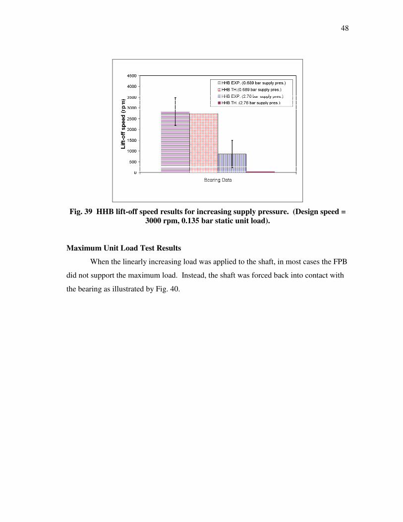
Fig. 39 HHB lift-off speed results for increasing supply pressure. (Design speed

= 3000 rpm, 0.135 bar static unit load). ............................................................. 48

Fig. 40 Lift-off, then contact in FPB (m = 0.27, 0.745 bar unit load, 0.689 bar

supply)................................................................................................................ 49

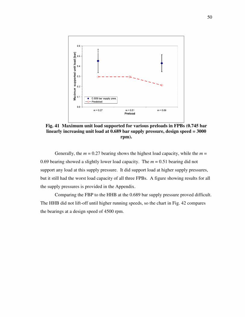
Fig. 41 Maximum unit load supported for various preloads in FPBs (0.745 bar

linearly increasing unit load at 0.689 bar supply pressure, design speed =

3000 rpm). .......................................................................................................... 50

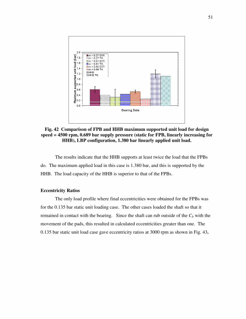
Fig. 42 Comparison of FPB and HHB maximum supported unit load for design

speed = 4500 rpm, 0.689 bar supply pressure (static for FPB, linearly

increasing for HHB), LBP configuration, 1.380 bar linearly applied unit

load. .................................................................................................................... 51

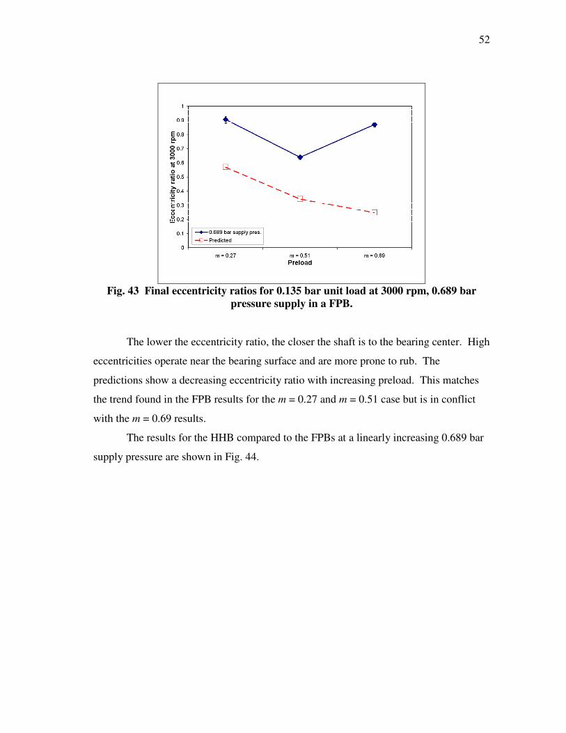
Fig. 43 Final eccentricity ratios for 0.135 bar unit load at 3000 rpm, 0.689 bar

pressure supply in a FPB.................................................................................... 52

xi

Page

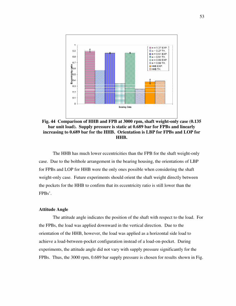
Fig. 44 Comparison of HHB and FPB at 3000 rpm, shaft weight-only case (0.135

bar unit load). Supply pressure is static at 0.689 bar for FPBs and linearly

increasing to 0.689 bar for the HHB. Orientation is LBP for FPBs and

LOP for HHB. .................................................................................................... 53

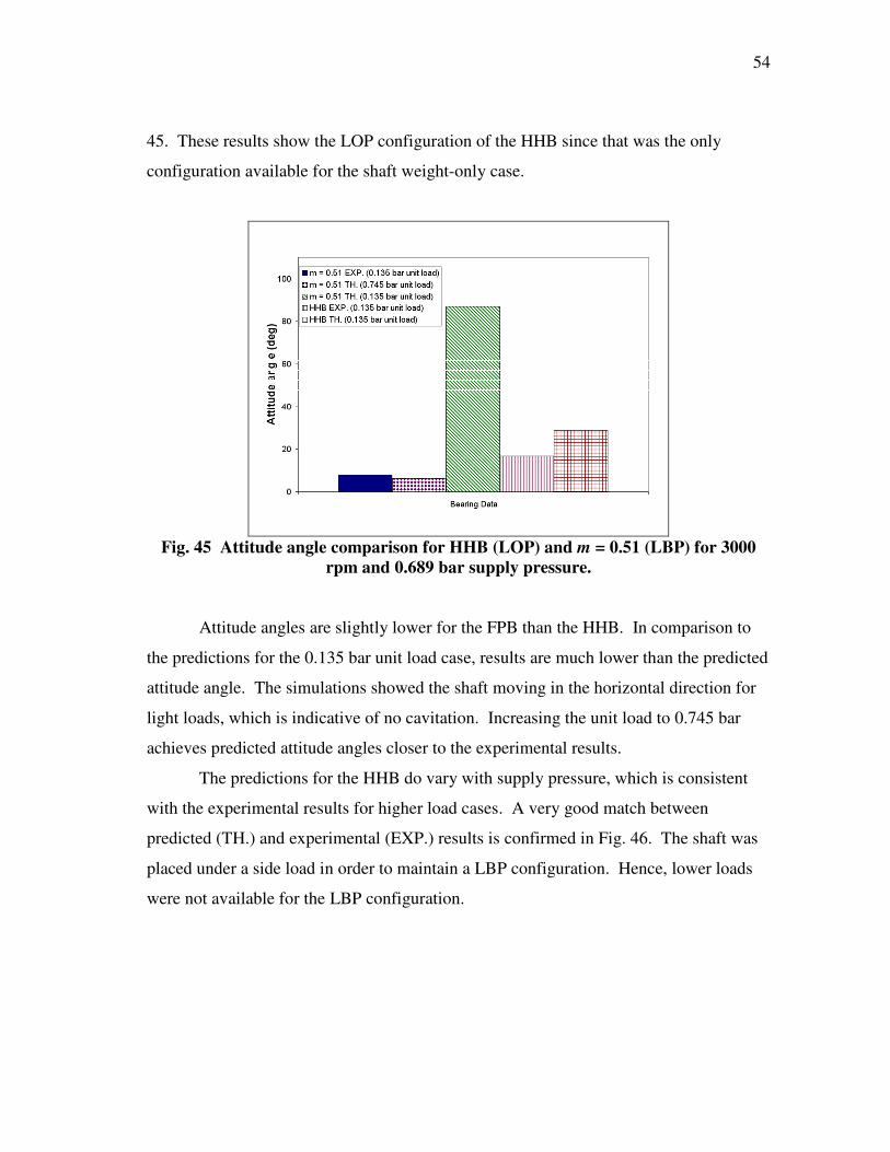
Fig. 45 Attitude angle comparison for HHB (LOP) and m = 0.51 (LBP) for 3000

rpm and 0.689 bar supply pressure. ................................................................... 54

Fig. 46 Comparison of HHB attitude angles (LBP, 0.745 bar unit load, 0.689 bar

supply)................................................................................................................ 55

Fig. 47 Simple beam definition. ..................................................................................... 62

Fig. 48 Maximum unit load supported for 0.745 bar linearly increasing unit load. ...... 64

Fig. 49 Eccentricity ratio at 3000 rpm for various preloads compared to

predictions. ......................................................................................................... 64

Fig. 50 Predicted lift-off comparison between water and kerosene (for constant

Cb). ..................................................................................................................... 65

Fig. 51 Predicted max unit load comparison between water and kerosene (for a

constant Cb). ....................................................................................................... 66

Fig. 52 Comparison of predicted eccentricity ratios between water and kerosene

(for a constant Cb). ............................................................................................. 66

Fig. 53 Comparison of predicted attitude angle for water and kerosene (m = 0.51,

0.745 bar unit load, constant Cb). ....................................................................... 67

xii

LIST OF TABLES

Page

Table 1 Bearing geometry from Scharrer et al. [16] .......................................................6

Table 2 Parameters for the flexure pivot pad support bearing predictions ...................11

Table 3 Properties of water at supply temperature = 104 °F (40 °C)............................12

Table 4 Designed FPBs .................................................................................................20

Table 5 Supply pressures and flowrates for FPB testing ..............................................22

Table 6 HHB geometry .................................................................................................22

Table 7 Measured average Cb........................................................................................31

Table 8 Manufactured clearances with tolerances ........................................................31

Table 9 Summary of measured clearances and preloads for FPBs ...............................32

Table 10 Comparison of water and kerosene ..................................................................55

Table 11 Reynolds numbers for water, kerosene, liquid methane ..................................56

Table 12 Beam calculation results ..................................................................................62

Table 13 Test matrix .......................................................................................................63

xiii

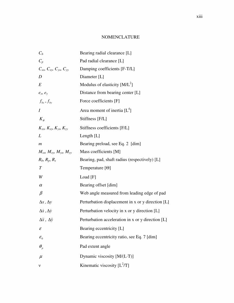
NOMENCLATURE

Cb Bearing radial clearance [L]

Cp Pad radial clearance [L]

Cxx, Cxy, Cyx, Cyy Damping coefficients [F-T/L]

D Diameter [L]

E Modulus of elasticity [M/L2]

ex, ey Distance from bearing center [L]

bxf , byf Force coefficients [F]

I Area moment of inertia [L4]

θK Stiffness [F/L]

Kxx, Kxy, Kyx, Kyy Stiffness coefficients [F/L]

L Length [L]

m Bearing preload, see Eq. 2 [dim]

Mxx, Mxy, Myx, Myy Mass coefficients [M]

Rb, Rp, Rs Bearing, pad, shaft radius (respectively) [L]

T Temperature [Θ]

W Load [F]

α Bearing offset [dim]

β Web angle measured from leading edge of pad

x∆ , y∆ Perturbation displacement in x or y direction [L]

x&∆ , y&∆ Perturbation velocity in x or y direction [L]

x&&∆ , y&&∆ Perturbation acceleration in x or y direction [L]

ε Bearing eccentricity [L]

0ε Bearing eccentricity ratio, see Eq. 7 [dim]

pθ Pad extent angle

µ Dynamic viscosity [M/(L·T)]

ν Kinematic viscosity [L2/T]

1

1. INTRODUCTION

High-speed turbopumps require reliable bearings to support the shaft or rotor.

One general type of bearing used in these applications is the hydrostatic bearing, which

uses external pressurization to inject fluid into the bearing. A restricting orifice creates

the pressure necessary to support the shaft in this type of bearing. The pocket pressure

supports the shaft even when there is no rotation.

On the other hand, hydrodynamic bearings do not use orifice restriction. A thin

fluid-film wedge develops as the shaft rotates, raising it off the bearing surface in a

process called lift-off [1]. Since there is no need for external pressurization,

hydrodynamic bearings eliminate a substantial cost to the end-user.

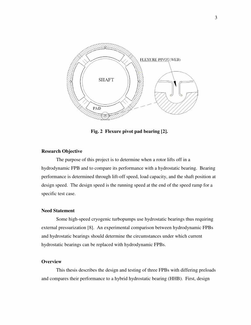
Bearing rotordynamic characteristics will be modeled using a combination of

stiffness, damping, and mass coefficients. The following linearized force-displacement

bearing model [2] is used for analysis:

∆

∆

+

∆

∆

+

∆

∆

=

−

y

x

MM

MM

y

x

CC

CC

y

x

KK

KK

f

f

yyyx

xyxx

yyyx

xyxx

yyyx

xyxx

by

bx

&&

&&

&

& (1)

The use of this linear model is a common practice in the analysis of rotor-bearing

systems [3]. Castigliano’s theorem states that a neutrally stable elastic system must have

a symmetric stiffness matrix [4]. The presence of skew-symmetric stiffness coefficients

indicates the presence of destabilizing forces [4]. Subsynchronous vibrations are one

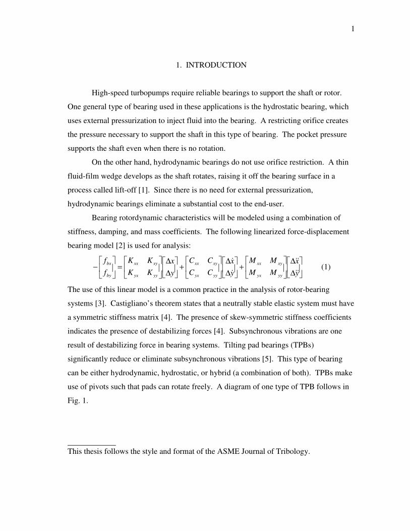
result of destabilizing force in bearing systems. Tilting pad bearings (TPBs)

significantly reduce or eliminate subsynchronous vibrations [5]. This type of bearing

can be either hydrodynamic, hydrostatic, or hybrid (a combination of both). TPBs make

use of pivots such that pads can rotate freely. A diagram of one type of TPB follows in

Fig. 1.

____________

This thesis follows the style and format of the ASME Journal of Tribology.

2

Fig. 1 Typical spherical seat TPB [6].

Even so, there are drawbacks to TPBs. These include wear at the pad pivot,

tolerance stack up due to a more complex design, reduced damping, and difficulty of

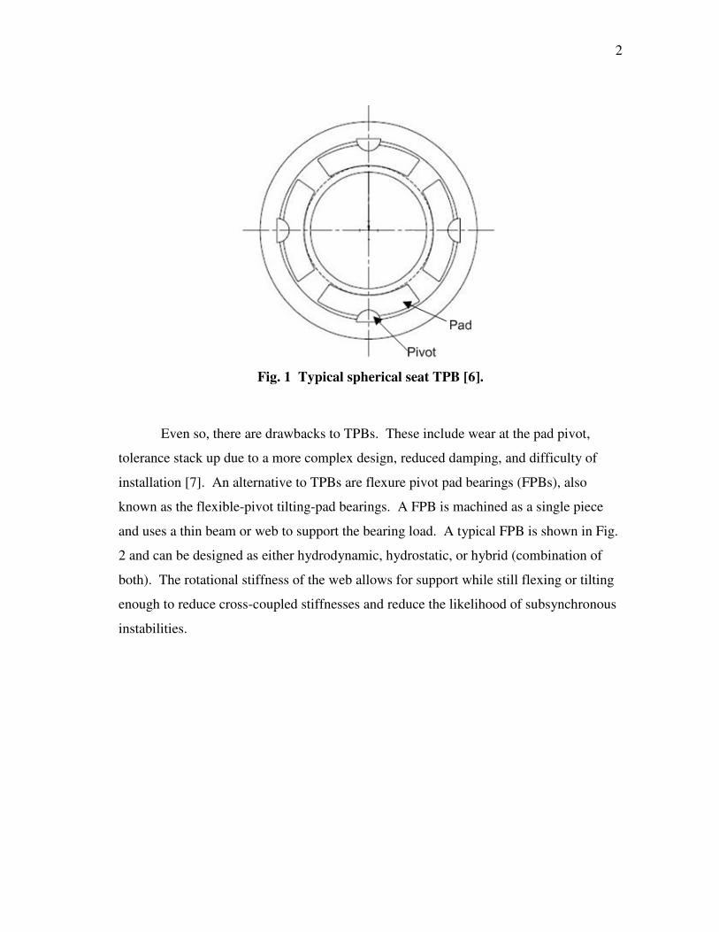
installation [7]. An alternative to TPBs are flexure pivot pad bearings (FPBs), also

known as the flexible-pivot tilting-pad bearings. A FPB is machined as a single piece

and uses a thin beam or web to support the bearing load. A typical FPB is shown in Fig.

2 and can be designed as either hydrodynamic, hydrostatic, or hybrid (combination of

both). The rotational stiffness of the web allows for support while still flexing or tilting

enough to reduce cross-coupled stiffnesses and reduce the likelihood of subsynchronous

instabilities.

3

Fig. 2 Flexure pivot pad bearing [2].

Research Objective

The purpose of this project is to determine when a rotor lifts off in a

hydrodynamic FPB and to compare its performance with a hydrostatic bearing. Bearing

performance is determined through lift-off speed, load capacity, and the shaft position at

design speed. The design speed is the running speed at the end of the speed ramp for a

specific test case.

Need Statement

Some high-speed cryogenic turbopumps use hydrostatic bearings thus requiring

external pressurization [8]. An experimental comparison between hydrodynamic FPBs

and hydrostatic bearings should determine the circumstances under which current

hydrostatic bearings can be replaced with hydrodynamic FPBs.

Overview

This thesis describes the design and testing of three FPBs with differing preloads

and compares their performance to a hybrid hydrostatic bearing (HHB). First, design

4

simulations are conducted using the XLTRCTM

Rotordynamics Suite (XLTRC2) [9]. By

varying specific design parameters that affect the load capacity of the bearing, it is

thought that the lift-off performance of the bearing will also be affected. After the

design is completed, the designed FPBs are manufactured and tested. An HHB is also

tested for comparison. Lift-off is determined from a shaft circuit voltage and verified

with waterfall and shaft centerline plots. All tested bearings are also simulated in

XLHydroJet® [10] to determine the validity of predicted results.

5

2. LITERATURE REVIEW

Early developments of the FPB by Zeidan and Paquette [7, 11] describe the

advantages of manufacturing a FPB versus a TPB. Due to their geometry, FPBs

eliminate tolerance stack up and pivot wear. There are no pads to install on the bearing

thus easing installation. Experiments conducted by De Choudhury et al. [12]

demonstrate that, in comparison to a similar five-pad TPB, a FPB operates at a lower

temperature and has less frictional power loss.

Since TPBs reduce cross-coupling, FPBs, similar to TPBs in geometry, should

also reduce cross-coupling and stabilize the system. Armentrout and Paquette [13]

showed that FPBs reduce destabilizing cross-coupling forces. For a four-pad FPB, with

L/D = 0.75 at 10,000 rpm, a pad rotational stiffness below 1,000 N-m (113.0 lb-in)

yields a bearing with cross-coupled stiffnesses comparable to TPBs. When the pad

stiffness is above 100,000 N-m (11,300 lb-in), a FPB acts like a fixed geometry bearing.

This leads to destabilizing cross-coupled stiffnesses. Evaluation of the pad web stresses

showed that, for an appropriately chosen geometry, the stresses on the pad web are too

small to degrade the lifetime due to fatigue.

Models

The physical modeling of FPBs is necessary for predicting their behavior in

operation. Early linear models of the bearing dynamic force coefficients by Chen [3]

confirmed the stability of a FPB. The method demonstrates that the support web must

be thick enough to carry the applied load and avoid fatigue, while at the same time being

flexible enough to mimic a TPB. San Andrés [8] introduced a bulk turbulent flow

thermal analysis of FPBs, specifically for cryogenic applications. The model shows a

reduced whirl frequency ratio (WFR) without loss in load capacity or reduction in direct

stiffness or damping. WFR is the ratio between the rotor natural frequency and the onset

speed of instability [1], and a lower WFR denotes a more stable bearing.

6

Effect of Varying Preload

An exact definition of preload, bearing clearance, and pad clearance can be found

in the Bearing Design section of this thesis. Elwell and Findlay [14] explored the

relationship between load capacity and bearing clearance in TPBs. Since preload is

related to bearing clearance, preload is also varied. Results for a laminar,

incompressible flow numerical solution of the Reynolds equation yield some insight into

the behavior of TPBs. They show that bearing load capacity increases with reduced

bearing clearance. However, the pad clearance seems to have little effect on the bearing

load capacity [14].

Others who conducted tests over a range of preloads include Wygant, et al. [15].

Their measurements indicated that preload does affect operating eccentricity but not

attitude angle. Operating eccentricity is the equilibrium position of the shaft in the

bearing for a fixed load, and attitude angle is the angle made by the center of the shaft

with respect to the center of the bearing [1].

Lift-off Testing

Scharrer et al. [16] conducted lift-off tests for hydrostatic bearings. These lift-off

experiments tested a hydrostatic journal bearing in a liquid nitrogen environment.

Several different bearings were used in testing, but the most common geometry is

provided in Table 1. The clearance ratio is a description of the bearing clearances as a

fraction of the total bearing radius. An exact definition of these terms is provided in the

Bearing Design section.

Table 1 Bearing geometry from Scharrer et al. [16]

Diameter 76.2 mm (3.0 in)

Length 31.75 mm (1.25 in)

Recesses 6

Clearance ratio (C b /R b ) 0.0267

7

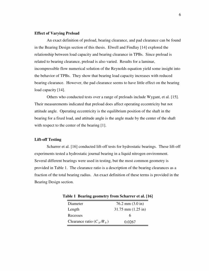
For these tests, Scharrer et al. [16] state that the reversal in shaft direction of rotation

from clockwise to counter-clockwise indicates the beginning of hydrodynamic lift-off, as

demonstrated in Fig. 3.

Fig. 3 Hydrodynamic lift-off from Scharrer et al. [16].

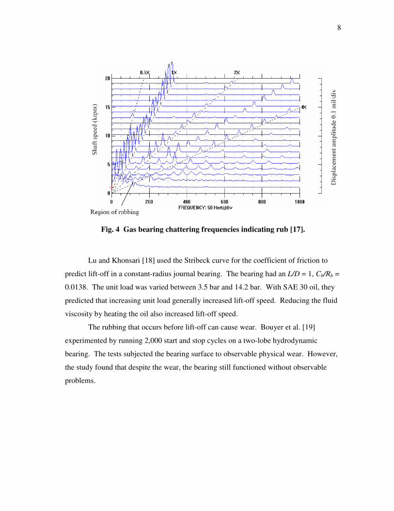
Zhu [17] performed tests for Rayleigh step gas bearings using waterfall plots to

identify the point after lift-off occurred. In gas bearings, metal to metal contact causes

chattering frequencies to develop which can be identified with waterfall plots. The point

where these chattering frequencies stop is the lift-off point. An example from Zhu’s

work can be seen in Fig. 4.

Inception of

hydrodynamic lift-off

8

Fig. 4 Gas bearing chattering frequencies indicating rub [17].

Lu and Khonsari [18] used the Stribeck curve for the coefficient of friction to

predict lift-off in a constant-radius journal bearing. The bearing had an L/D = 1, Cb/Rb =

0.0138. The unit load was varied between 3.5 bar and 14.2 bar. With SAE 30 oil, they

predicted that increasing unit load generally increased lift-off speed. Reducing the fluid

viscosity by heating the oil also increased lift-off speed.

The rubbing that occurs before lift-off can cause wear. Bouyer et al. [19]

experimented by running 2,000 start and stop cycles on a two-lobe hydrodynamic

bearing. The tests subjected the bearing surface to observable physical wear. However,

the study found that despite the wear, the bearing still functioned without observable

problems.

9

3. BEARING DESIGN

The first step in the design of the bearing was to determine which parameter had

the most significant effect on lift-off. The simulations do not predict lift-off. Instead,

they calculate the film thickness developed in the bearing. For the design simulations,

the maximum load capacity of the bearing is defined to be the load where the minimum

film thickness is equal to twice the surface roughness of the rotor. At this point, rubbing

is assumed to occur between the rotor and bearing. For a typical turning manufacturing

process, the surface roughness is approximately 2 µm (0.08 mils) [20]. Using these

definitions, both preload and offset are varied to discover their effect on bearing load

capacity. This definition is used in all the simulations to determine the load capacity.

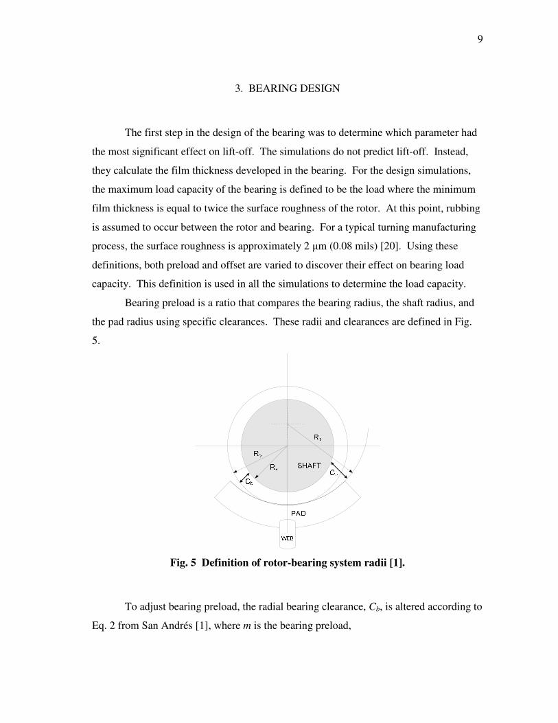
Bearing preload is a ratio that compares the bearing radius, the shaft radius, and

the pad radius using specific clearances. These radii and clearances are defined in Fig.

5.

Fig. 5 Definition of rotor-bearing system radii [1].

To adjust bearing preload, the radial bearing clearance, Cb, is altered according to

Eq. 2 from San Andrés [1], where m is the bearing preload,

10

p

b

C

Cm −= 1 . (2)

The following relationships describe the clearances:

sbb RRC −= , (3)

spp RRC −= . (4)

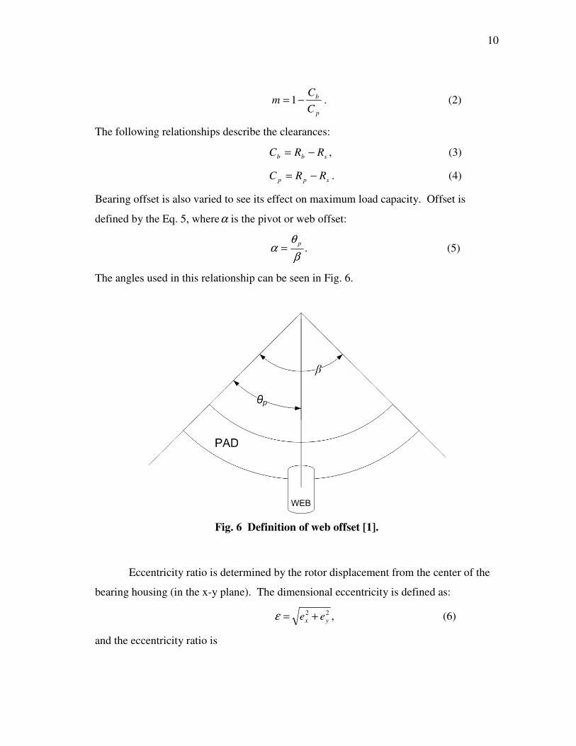
Bearing offset is also varied to see its effect on maximum load capacity. Offset is

defined by the Eq. 5, whereα is the pivot or web offset:

.β

θα

p= (5)

The angles used in this relationship can be seen in Fig. 6.

Fig. 6 Definition of web offset [1].

Eccentricity ratio is determined by the rotor displacement from the center of the

bearing housing (in the x-y plane). The dimensional eccentricity is defined as:

,22

yx ee +=ε (6)

and the eccentricity ratio is

11

.0

bC

εε = (7)

The bearing clearance, Cb, is the minimum clearance where contact could occur. Thus a

ratio equal to one would refer to contact with the bearing surface, and a ratio equal to

zero would be a perfectly centered bearing.

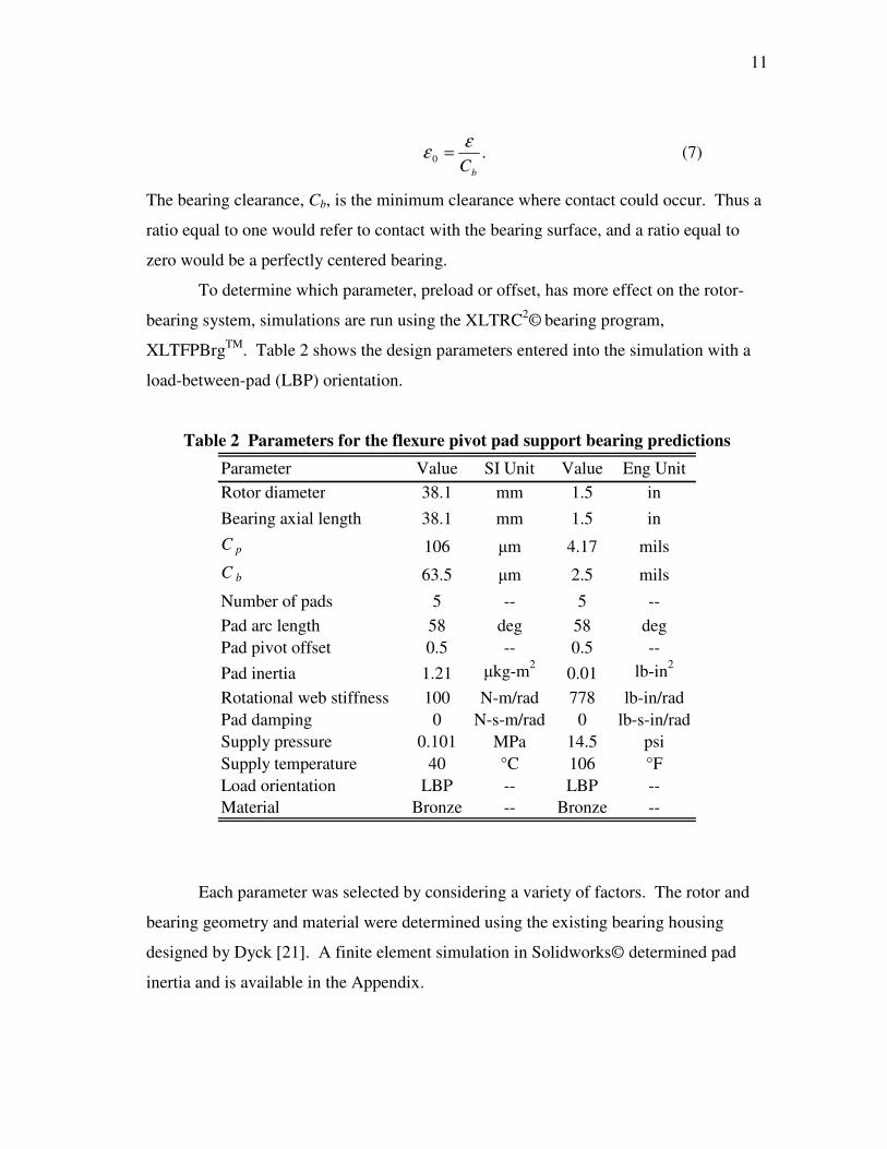
To determine which parameter, preload or offset, has more effect on the rotor-

bearing system, simulations are run using the XLTRC2©

bearing program,

XLTFPBrgTM

. Table 2 shows the design parameters entered into the simulation with a

load-between-pad (LBP) orientation.

Table 2 Parameters for the flexure pivot pad support bearing predictions

Parameter Value SI Unit Value Eng Unit

Rotor diameter 38.1 mm 1.5 in

Bearing axial length 38.1 mm 1.5 in

C p 106 µm 4.17 mils

C b 63.5 µm 2.5 mils

Number of pads 5 -- 5 --

Pad arc length 58 deg 58 deg

Pad pivot offset 0.5 -- 0.5 --

Pad inertia 1.21 µkg-m2

0.01 lb-in2

Rotational web stiffness 100 N-m/rad 778 lb-in/rad

Pad damping 0 N-s-m/rad 0 lb-s-in/rad

Supply pressure 0.101 MPa 14.5 psi

Supply temperature 40 °C 106 °F

Load orientation LBP -- LBP --

Material Bronze -- Bronze --

Each parameter was selected by considering a variety of factors. The rotor and

bearing geometry and material were determined using the existing bearing housing

designed by Dyck [21]. A finite element simulation in Solidworks© determined pad

inertia and is available in the Appendix.

12

The selected pad stiffness came from the recommended pad rotational stiffness of

1.13 – 11,300 N-m/rad (10 – 100,000 lb-in/rad) set forth by Kepple et al. [5]. They used

a 50.89 mm (2.0035 in) diameter bearing with Cb/Rb = 0.00175. The proposed bearing

has a diameter of 38.23 mm (1.505 in) with Cb/Rb = 0.00333. The difference in these

bearings is small so using a moderate pad rotational stiffness within this range should be

acceptable. If the pad stiffness exceeds the recommended upper limit, the web no longer

deflects enough for the bearing to behave as a TPB, and the cross-coupled stiffnesses

increase significantly. Selecting a lower stiffness further decreases the possibility of

instabilities due to cross coupling.

The clearances were selected by choosing a specific preload and offset. The

number of pads, pad stiffness, and load orientation were also varied slightly to see their

effect on the system. These results will be discussed after noting the effect of preload

and offset.

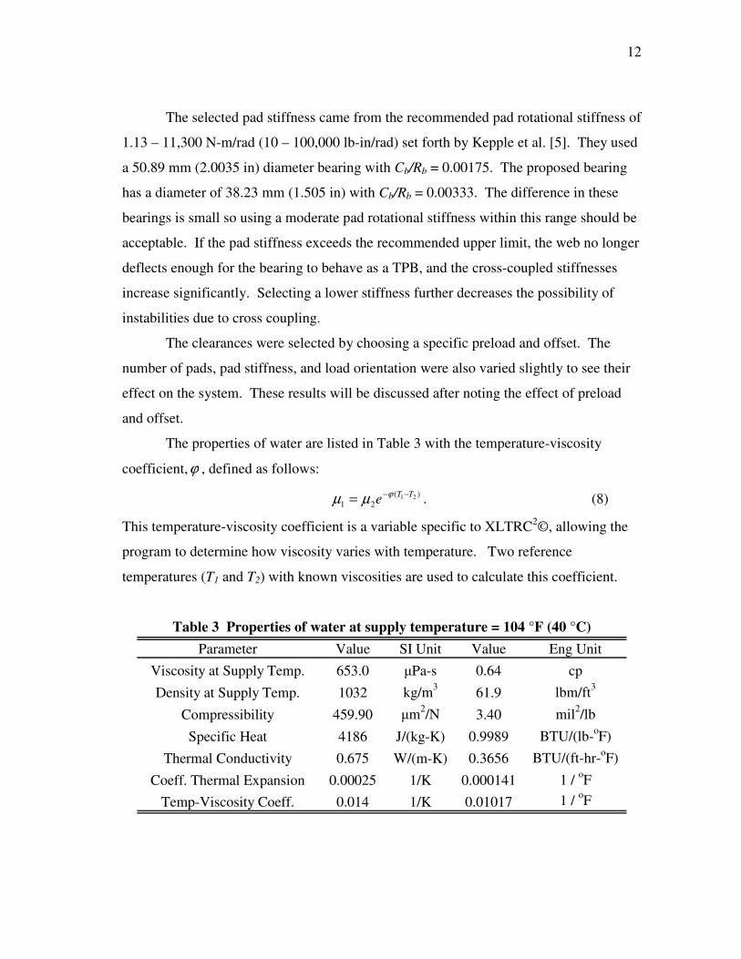
The properties of water are listed in Table 3 with the temperature-viscosity

coefficient,ϕ , defined as follows:

)(

2121 TT

e−−= ϕµµ . (8)

This temperature-viscosity coefficient is a variable specific to XLTRC2©, allowing the

program to determine how viscosity varies with temperature. Two reference

temperatures (T1 and T2) with known viscosities are used to calculate this coefficient.

Table 3 Properties of water at supply temperature = 104 °F (40 °C)

Parameter Value SI Unit Value Eng Unit

Viscosity at Supply Temp. 653.0 µPa-s 0.64 cp

Density at Supply Temp. 1032 kg/m3

61.9 lbm/ft3

Compressibility 459.90 µm2/N 3.40 mil

2/lb

Specific Heat 4186 J/(kg-K) 0.9989 BTU/(lb-oF)

Thermal Conductivity 0.675 W/(m-K) 0.3656 BTU/(ft-hr-oF)

Coeff. Thermal Expansion 0.00025 1/K 0.000141 1 / oF

Temp-Viscosity Coeff. 0.014 1/K 0.01017 1 / oF

13

Effect of Preload and Offset

When preload is changed, the clearances in the bearing change, affecting the

behavior of the fluid film. Since this fluid film supports the bearing, the load capacity of

the bearing should also be affected by changes in the preload. Typical values of preload

range from 0.2 to 0.6. Beyond 0.6, San Andrés [1] found that frictional losses are high,

rendering the bearing impractical.

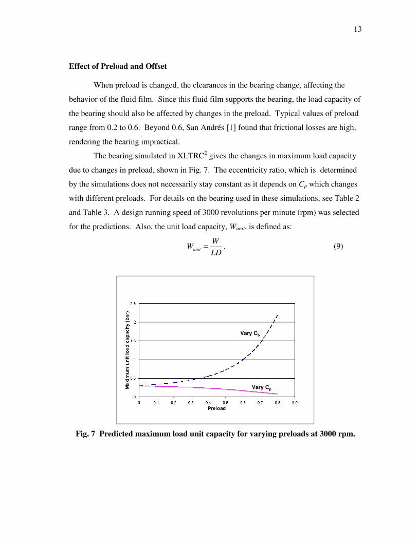
The bearing simulated in XLTRC2 gives the changes in maximum load capacity

due to changes in preload, shown in Fig. 7. The eccentricity ratio, which is determined

by the simulations does not necessarily stay constant as it depends on Cp which changes

with different preloads. For details on the bearing used in these simulations, see Table 2

and Table 3. A design running speed of 3000 revolutions per minute (rpm) was selected

for the predictions. Also, the unit load capacity, Wunit, is defined as:

LD

WWunit = . (9)

Vary Cp

Vary Cb

Fig. 7 Predicted maximum load unit capacity for varying preloads at 3000 rpm.

14

Two different methods of varying preload were conducted, as shown in Fig. 7.

The purpose of this figure is to illustrate that changing the preload does change the load

capacity of the bearing. The first method for illustrating a changing load capacity holds

Cp constant and varies Cb. This moves the entire pad closer to the rotor, changing the

preload. The predicted results for this method shown with a dotted line indicate that

load capacity increases quickly with increasing preload. Trends simulated by Elwell and

Findlay [14] agree with this result—a smaller Cb yields a greater load capacity.

The other method holds Cb constant and varies Cp. This changes the curvature of

the pad in order to change preload. Since Cb determines the minimum bearing clearance,

changing Cp is more practical from a manufacturing standpoint. Each FPB will be

compared to a HHB with no preload. The FPB must also have the same minimum

clearance, or Cb, as the HHB. To change preload for the different FPBs, then, Cp will be

changed. As shown in the solid line in Fig. 7, the maximum load capacity decreases

gradually when increasing preload in this manner. Elwell and Findlay [14] found no

effect on the load capacity for an increasing Cp.

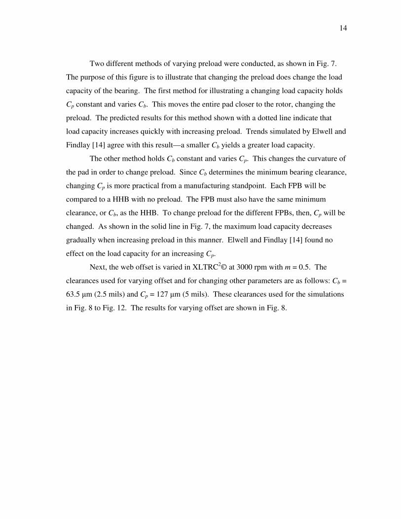
Next, the web offset is varied in XLTRC2© at 3000 rpm with m = 0.5. The

clearances used for varying offset and for changing other parameters are as follows: Cb =

63.5 µm (2.5 mils) and Cp = 127 µm (5 mils). These clearances used for the simulations

in Fig. 8 to Fig. 12. The results for varying offset are shown in Fig. 8.

15

Fig. 8 Predicted maximum unit load capacity for varying offsets.

As the offset increases, the maximum load capacity also increases. However,

this value peaks at relatively small value. The total change in load capacity is

significantly less for a varying offset than for a varying preload. Thus, for reasonable

ranges in both preload and offset, changing the preload would have more effect on the

load capacity of the bearing than changing the offset. This is true regardless of the way

the preload is varied.

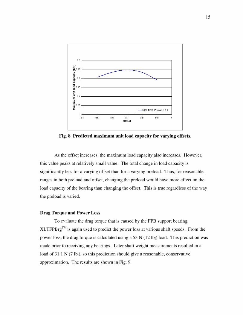
Drag Torque and Power Loss

To evaluate the drag torque that is caused by the FPB support bearing,

XLTFPBrgTM

is again used to predict the power loss at various shaft speeds. From the

power loss, the drag torque is calculated using a 53 N (12 lbf) load. This prediction was

made prior to receiving any bearings. Later shaft weight measurements resulted in a

load of 31.1 N (7 lbf), so this prediction should give a reasonable, conservative

approximation. The results are shown in Fig. 9.

16

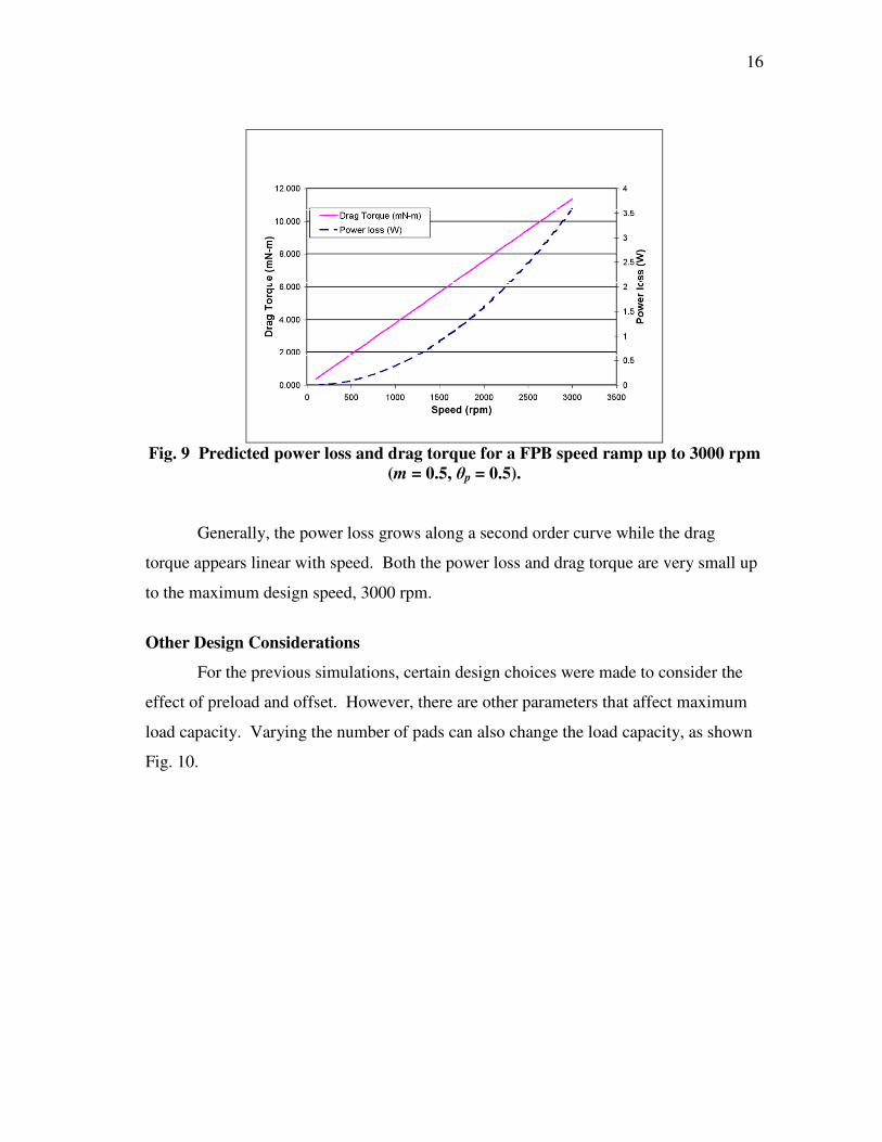
Fig. 9 Predicted power loss and drag torque for a FPB speed ramp up to 3000 rpm

(m = 0.5, θp = 0.5).

Generally, the power loss grows along a second order curve while the drag

torque appears linear with speed. Both the power loss and drag torque are very small up

to the maximum design speed, 3000 rpm.

Other Design Considerations

For the previous simulations, certain design choices were made to consider the

effect of preload and offset. However, there are other parameters that affect maximum

load capacity. Varying the number of pads can also change the load capacity, as shown

Fig. 10.

17

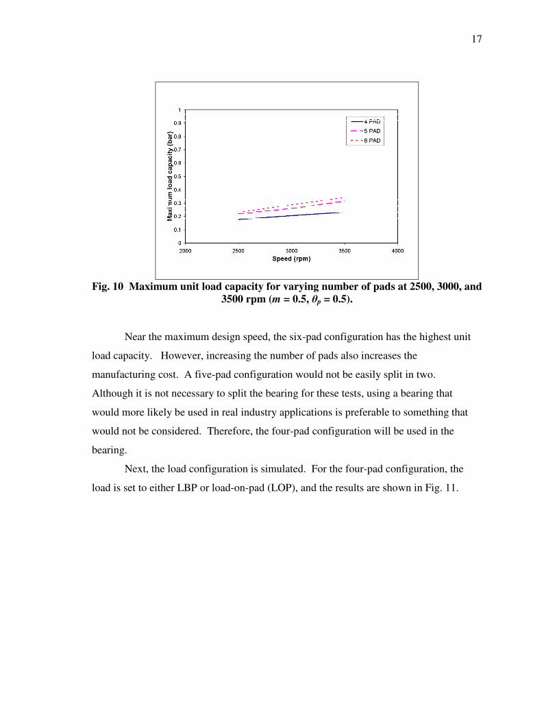
Fig. 10 Maximum unit load capacity for varying number of pads at 2500, 3000, and

3500 rpm (m = 0.5, θp = 0.5).

Near the maximum design speed, the six-pad configuration has the highest unit

load capacity. However, increasing the number of pads also increases the

manufacturing cost. A five-pad configuration would not be easily split in two.

Although it is not necessary to split the bearing for these tests, using a bearing that

would more likely be used in real industry applications is preferable to something that

would not be considered. Therefore, the four-pad configuration will be used in the

bearing.

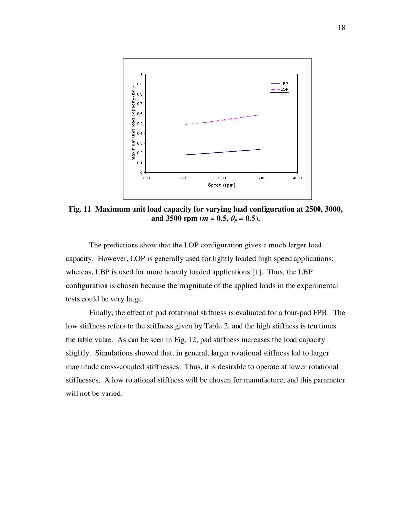
Next, the load configuration is simulated. For the four-pad configuration, the

load is set to either LBP or load-on-pad (LOP), and the results are shown in Fig. 11.

18

Fig. 11 Maximum unit load capacity for varying load configuration at 2500, 3000,

and 3500 rpm (m = 0.5, θp = 0.5).

The predictions show that the LOP configuration gives a much larger load

capacity. However, LOP is generally used for lightly loaded high speed applications;

whereas, LBP is used for more heavily loaded applications [1]. Thus, the LBP

configuration is chosen because the magnitude of the applied loads in the experimental

tests could be very large.

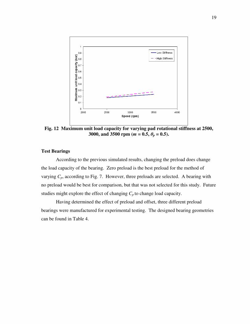
Finally, the effect of pad rotational stiffness is evaluated for a four-pad FPB. The

low stiffness refers to the stiffness given by Table 2, and the high stiffness is ten times

the table value. As can be seen in Fig. 12, pad stiffness increases the load capacity

slightly. Simulations showed that, in general, larger rotational stiffness led to larger

magnitude cross-coupled stiffnesses. Thus, it is desirable to operate at lower rotational

stiffnesses. A low rotational stiffness will be chosen for manufacture, and this parameter

will not be varied.

19

Fig. 12 Maximum unit load capacity for varying pad rotational stiffness at 2500,

3000, and 3500 rpm (m = 0.5, θp = 0.5).

Test Bearings

According to the previous simulated results, changing the preload does change

the load capacity of the bearing. Zero preload is the best preload for the method of

varying Cp, according to Fig. 7. However, three preloads are selected. A bearing with

no preload would be best for comparison, but that was not selected for this study. Future

studies might explore the effect of changing Cp to change load capacity.

Having determined the effect of preload and offset, three different preload

bearings were manufactured for experimental testing. The designed bearing geometries

can be found in Table 4.

20

Table 4 Designed FPBs

Preload 0.3 0.5 0.7 Unit

Radial axial length 38.1 (1.5) 38.1 (1.5) 38.1 (1.5) mm (in)

C p 90.71 (3.57) 127.00 (5.00) 211.67 (8.33) µm (mils)

C b 63.5 (2.50) 63.5 (2.50) 63.5 (2.50) µm (mils)

Offset 0.5 0.5 0.5

Number of pads 4 4 4 --

Pad arc length 72 72 72 deg

Pad pivot offset 0.5 0.5 0.5 --

Material 660 bearing bronze 660 bearing bronze 660 bearing bronze

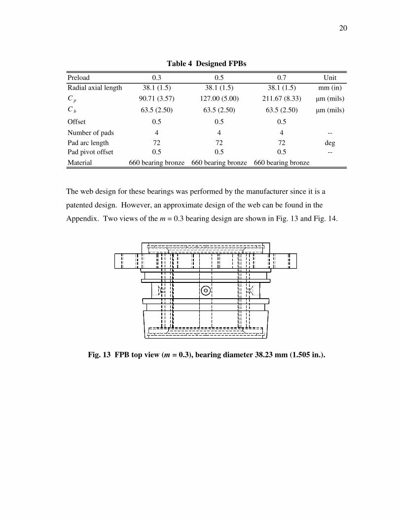
The web design for these bearings was performed by the manufacturer since it is a

patented design. However, an approximate design of the web can be found in the

Appendix. Two views of the m = 0.3 bearing design are shown in Fig. 13 and Fig. 14.

Fig. 13 FPB top view (m = 0.3), bearing diameter 38.23 mm (1.505 in.).

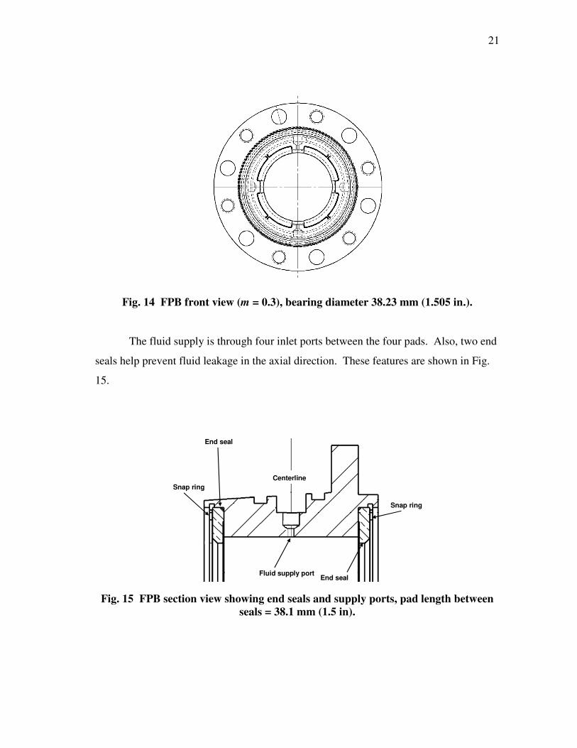
21

Fig. 14 FPB front view (m = 0.3), bearing diameter 38.23 mm (1.505 in.).

The fluid supply is through four inlet ports between the four pads. Also, two end

seals help prevent fluid leakage in the axial direction. These features are shown in Fig.

15.

Snap ring

Snap ring

End seal

End sealFluid supply port

Centerline

Fig. 15 FPB section view showing end seals and supply ports, pad length between

seals = 38.1 mm (1.5 in).

22

During testing of the FPBs, the fluid supply pressure was varied. Three different

fluid supply pressures were used with different flowrates. These supply pressures and

corresponding flowrates are shown in Table 5.

Table 5 Supply pressures and flowrates for FPB testing

Supply pressure (bar) Flowrate (lpm)

0.69 (10 psia) 5.68 (1.5 gpm)

2.76 (40 psia) 10.22 (2.7 gpm)

5.52 (80 psia) 13.63 (3.6 gpm)

In addition, one six pocket HHB was manufactured for comparison with FPBs,

and its details can be found in Table 6.

Table 6 HHB geometry

Parameter Value Unit

Bearing axial length 38.1 (1.5) mm (in)

Radial bearing clearance 63.5 (2.50) µm (mils)

Number of pockets 6 --

Pocket axial length 11.97 (0.47) mm (in)

Pocket depth 406 (16) µm (mils)

Orifice diameter 1.397 (0.055) mm (in)

Orifice location relative to pocket (%) 50 --

Material 660 Bearing Bronze --

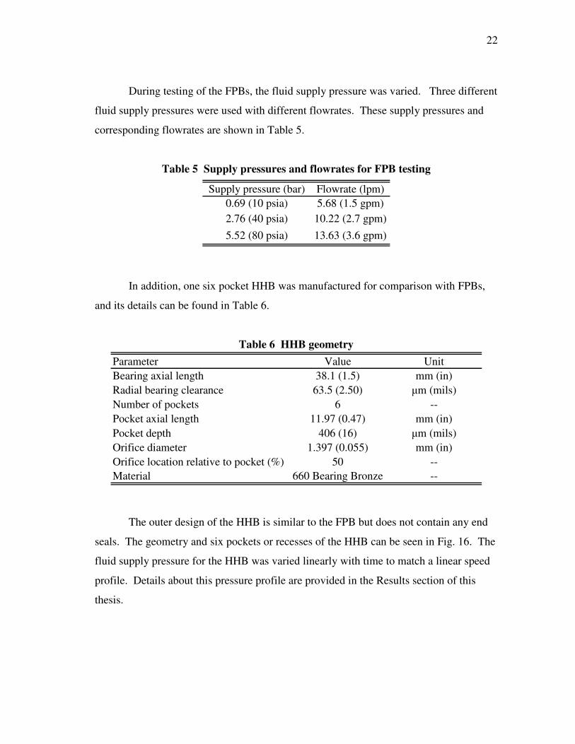
The outer design of the HHB is similar to the FPB but does not contain any end

seals. The geometry and six pockets or recesses of the HHB can be seen in Fig. 16. The

fluid supply pressure for the HHB was varied linearly with time to match a linear speed

profile. Details about this pressure profile are provided in the Results section of this

thesis.

23

Bearing pad pressure port

Fluid supply port

Recess

Fig. 16 HHB geometry with supply ports and recesses shown.

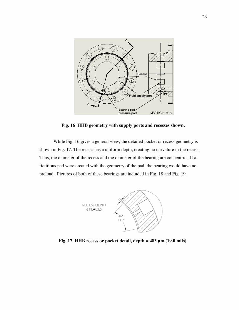
While Fig. 16 gives a general view, the detailed pocket or recess geometry is

shown in Fig. 17. The recess has a uniform depth, creating no curvature in the recess.

Thus, the diameter of the recess and the diameter of the bearing are concentric. If a

fictitious pad were created with the geometry of the pad, the bearing would have no

preload. Pictures of both of these bearings are included in Fig. 18 and Fig. 19.

Fig. 17 HHB recess or pocket detail, depth = 483 µm (19.0 mils).

24

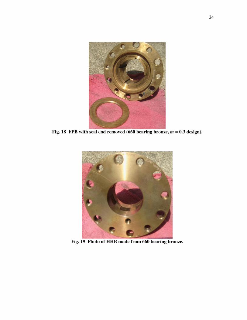
Fig. 18 FPB with seal end removed (660 bearing bronze, m = 0.3 design).

Fig. 19 Photo of HHB made from 660 bearing bronze.

25

4. EXPERIMENTAL PROCEDURE

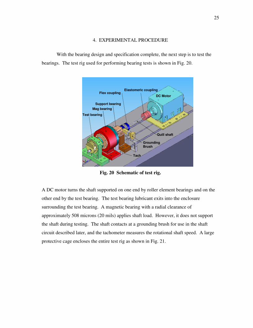
With the bearing design and specification complete, the next step is to test the

bearings. The test rig used for performing bearing tests is shown in Fig. 20.

Test bearing

Mag bearing

Grounding Brush

Support bearing

Tach

Flex couplingElastomeric coupling

DC Motor

Quill shaft

Fig. 20 Schematic of test rig.

A DC motor turns the shaft supported on one end by roller element bearings and on the

other end by the test bearing. The test bearing lubricant exits into the enclosure

surrounding the test bearing. A magnetic bearing with a radial clearance of

approximately 508 microns (20 mils) applies shaft load. However, it does not support

the shaft during testing. The shaft contacts at a grounding brush for use in the shaft

circuit described later, and the tachometer measures the rotational shaft speed. A large

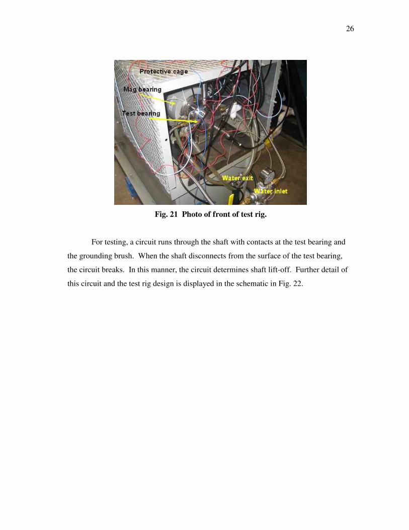
protective cage encloses the entire test rig as shown in Fig. 21.

26

Fig. 21 Photo of front of test rig.

For testing, a circuit runs through the shaft with contacts at the test bearing and

the grounding brush. When the shaft disconnects from the surface of the test bearing,

the circuit breaks. In this manner, the circuit determines shaft lift-off. Further detail of

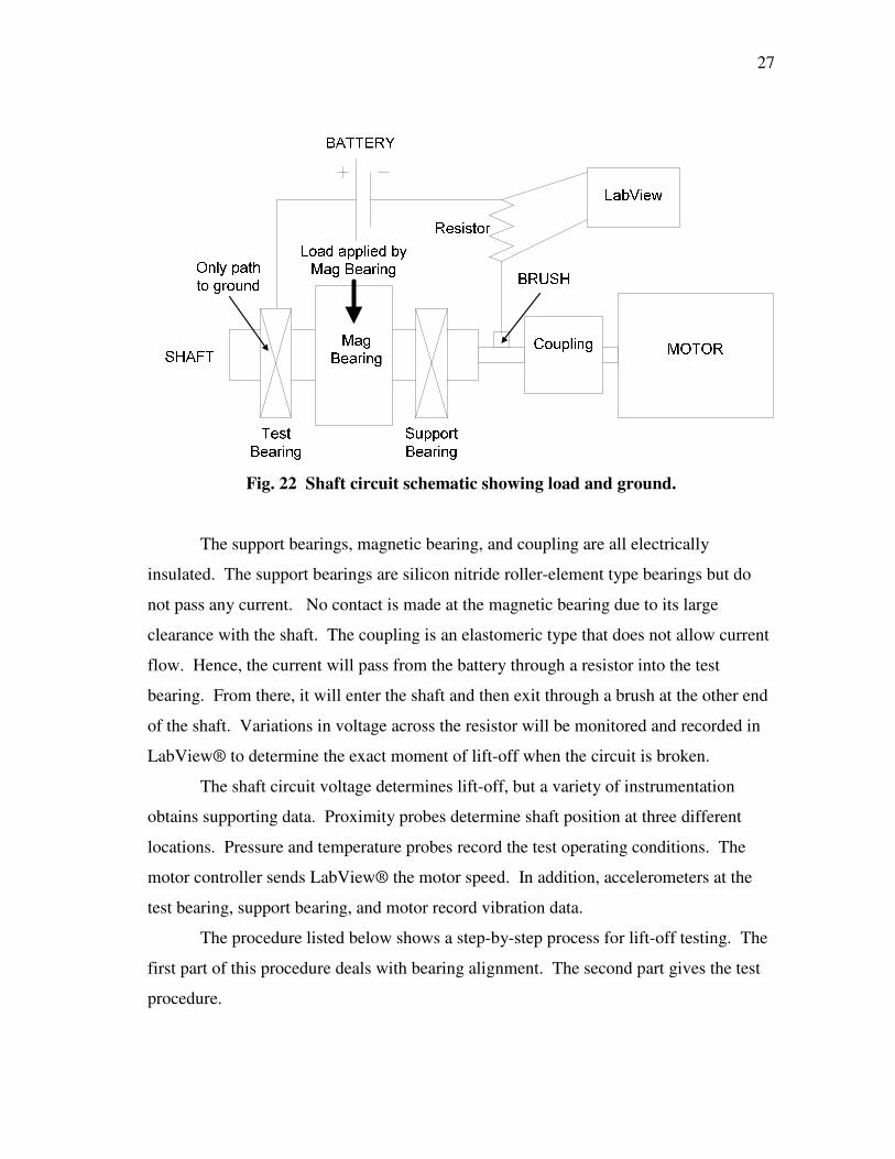
this circuit and the test rig design is displayed in the schematic in Fig. 22.

27

Fig. 22 Shaft circuit schematic showing load and ground.

The support bearings, magnetic bearing, and coupling are all electrically

insulated. The support bearings are silicon nitride roller-element type bearings but do

not pass any current. No contact is made at the magnetic bearing due to its large

clearance with the shaft. The coupling is an elastomeric type that does not allow current

flow. Hence, the current will pass from the battery through a resistor into the test

bearing. From there, it will enter the shaft and then exit through a brush at the other end

of the shaft. Variations in voltage across the resistor will be monitored and recorded in

LabView® to determine the exact moment of lift-off when the circuit is broken.

The shaft circuit voltage determines lift-off, but a variety of instrumentation

obtains supporting data. Proximity probes determine shaft position at three different

locations. Pressure and temperature probes record the test operating conditions. The

motor controller sends LabView® the motor speed. In addition, accelerometers at the

test bearing, support bearing, and motor record vibration data.

The procedure listed below shows a step-by-step process for lift-off testing. The

first part of this procedure deals with bearing alignment. The second part gives the test

procedure.

28

Bearing Alignment Procedure

1) Install bearing into the test pedestal by tightening the insertion bolts all the way

in.

2) Loosen the insertion bolts and insert 50.8 µm (2.0 mil) shims at four positions on

the bearing (on the pad if applicable). Note that the magnitude of shimming

depends on bearing clearance.

3) Tighten bolts and lock bearing with locking bolts.

4) Measure depth with a micrometer-type depth gauge at three points around the

bearing face to ensure there is no cocking of the bearing in the test pedestal. The

depth at each of these three points should be within 12.7 µm (0.5 mil) of each

other.

5) Remove the shims from between the shaft and the bearing.

6) Close the test bearing pedestal with the outer housing and install proximity

probes to proper depth.

7) Energize the magnetic bearing and enter calibration factors for loading.

8) While recording bearing position data in LabView®, load the shaft in a manner

to bump it against the bearing surface. Repeat these bump tests in every

direction until a clear picture of the bearing clearance is formed.

9) Determine bearing clearance from the bump test data in both the X and Y

directions.

10) The bearing alignment is complete if the X and Y calculated clearances are within

25.4 µm (1 mil) of each other. This ensures the shaft is centered and can move

freely.

Test Procedure

1) Turn on the pump to buffer water to the test bearing.

2) Turn on air to the air seal that prevents water flowing axially to the magnetic

bearing.

29

3) Establish a flow of water to the bearing based on the supply pressure specified by

the test case. The test matrix showing all test cases is shown in the Appendix.

4) Begin LabView® data acquisition.

5) Turn on the motor and accelerate to the design speed with the load and pressure

profile given by the specific test case.

6) Record data to both a binary file and a spreadsheet.

7) Stop the motor and repeat each test case until 10 iterations of current test case are

completed.

8) Proceed to next test case. If all test cases are complete for current bearing, turn

off water and repeat bump test as described in the bearing alignment procedure.

This will determine if the bearing has moved substantially during testing.

9) Remove current bearing and observe wear.

10) Proceed to next bearing and repeat bearing alignment procedure and test

procedure.

Bearing Clearance Measurement

In FPBs, the bearing clearance (Cb) is the minimum clearance in the bearing, thus

it will be used to determine bearing eccentricity and preload. Typically, one could place

the shaft in contact with the center of one pad and then move it to the center of the

opposing pad to determine bearing clearance from the displacement. However, due to

the setup of the test rig, the test bearing could only be mounted in the LBP position.

This prevented a simple shaft up and down bump test to determine bearing clearance.

Loading the shaft at a 45° angle to attempt load-on-pad proved unmanageable for

determining bearing clearance. When load was applied at an angle, the shaft slipped off

the pad to one of the LBP pad positions.

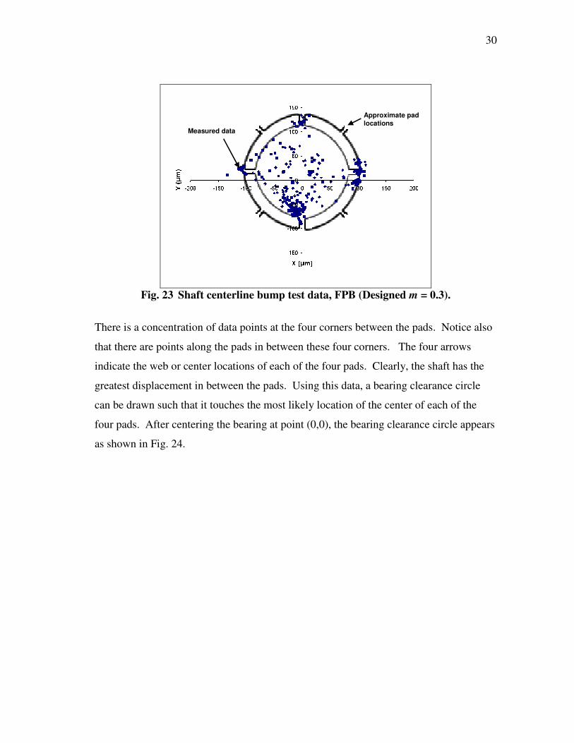
Instead of trying to load directly on the pad, bump tests were performed over the

bearing circumference for eight different load directions. Loads covered the horizontal,

vertical, and 45° diagonals in the bearing. An example of the resulting data is shown in

Fig. 23.

30

Measured data

Approximate pad locations

Fig. 23 Shaft centerline bump test data, FPB (Designed m = 0.3).

There is a concentration of data points at the four corners between the pads. Notice also

that there are points along the pads in between these four corners. The four arrows

indicate the web or center locations of each of the four pads. Clearly, the shaft has the

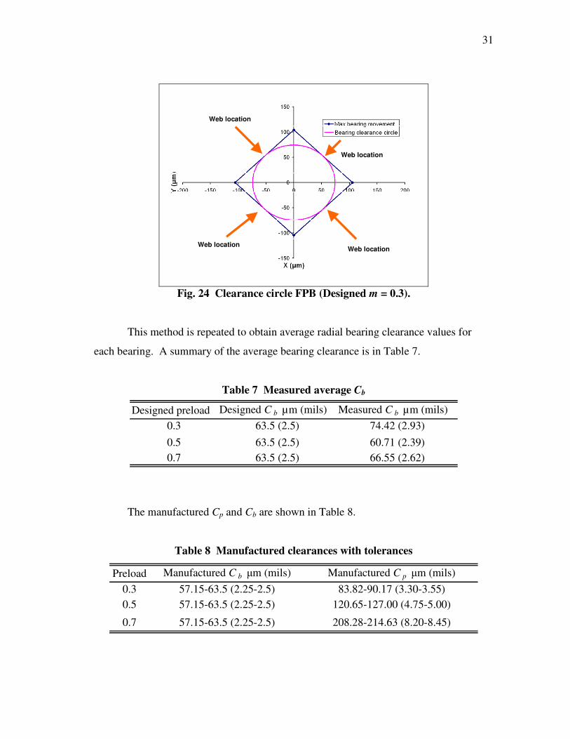
greatest displacement in between the pads. Using this data, a bearing clearance circle

can be drawn such that it touches the most likely location of the center of each of the

four pads. After centering the bearing at point (0,0), the bearing clearance circle appears

as shown in Fig. 24.

31

Web location

Web location

Web location

Web location

Fig. 24 Clearance circle FPB (Designed m = 0.3).

This method is repeated to obtain average radial bearing clearance values for

each bearing. A summary of the average bearing clearance is in Table 7.

Table 7 Measured average Cb

Designed preload Designed C b µm (mils) Measured C b µm (mils)

0.3 63.5 (2.5) 74.42 (2.93)

0.5 63.5 (2.5) 60.71 (2.39)

0.7 63.5 (2.5) 66.55 (2.62)

The manufactured Cp and Cb are shown in Table 8.

Table 8 Manufactured clearances with tolerances

Preload Manufactured C b µm (mils) Manufactured C p µm (mils)

0.3 57.15-63.5 (2.25-2.5) 83.82-90.17 (3.30-3.55)

0.5 57.15-63.5 (2.25-2.5) 120.65-127.00 (4.75-5.00)

0.7 57.15-63.5 (2.25-2.5) 208.28-214.63 (8.20-8.45)

32

Using the upper end of the tolerance range, the difference between Cp and Cb is

calculated for the given manufactured clearances. This difference is then used to

calculate a new preload for each bearing. A new Cp is calculated by adding this

difference to the average measured Cb. From these values, a preload can be calculated

according to Eq. 2. The resulting measured preloads and clearances are summarized in

Table 9.

Table 9 Summary of measured clearances and preloads for FPBs

Designed preload Measured C b µm (mils) Calculated C p µm (mils) New preload

0.3 74.42 (2.93) 101.63 (4.00) 0.27

0.5 60.71 (2.39) 124.21 (4.89) 0.51

0.7 66.55 (2.62) 214.72 (8.45) 0.69

The actual measured Cb for the HHB is different from the value given by the

manufacturer. The given Cb is 63.5 ± 2.5 µm (2.5 ± 0.1 mils). However, the measured

value according to the procedure determined above was 59.1 µm (2.327 mils). The

measured values for the clearances and preloads of all the bearings will be used in the

Results section.

Lift-off Determination

There are three methods used in this paper for determining and confirming lift-

off. First, the shaft circuit voltage is monitored for disturbances indicating lift-off. This

was by far the most successful method. It achieved repeatable results within several

hundred rpm. Considering the rapid acceleration of the shaft (0 to 4500 rpm in

approximately 0.84s), this is a highly accurate result.

Second, waterfall plots are made of the accelerometer data showing vibrations in

the test pedestal. Larger vibration amplitudes are observed during bearing rubbing than

when it has lifted off. This second method has been used in air bearings and evaluates

33

waterfall plots of the displacement data [19]. A chattering frequency at low speeds

occurs when there is metal-to-metal contact. This method yielded some accurate results

but lacked consistency in testing. The exact point of lift-off was harder to determine due

to several different high frequencies to watch during bearing rub.

Finally, since the bearing clearance defines the shaft position relative to the

bearing surface, shaft centerline plots can be used to verify lift-off. Centerline plots

depend on the definition of the bearing surface. Since there is some uncertainty in

determining the bearing clearance, exact lift-off speeds will also have some uncertainty

when calculated by this method.

After consideration of the three methods described, the most repeatable and

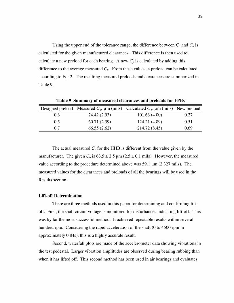
accurate indicator of lift-off comes from variation in the shaft voltage. For the example

given in Fig. 25, there is a clear drop of about 0.25 volts as the shaft rises from the

bearing housing.

Initial Steady Voltage

Motor Speed

Shaft approaches equilibrium position

Lifting

Noise at initial lift-off

Clear lift-off identified

Fig. 25 Lift-off voltage for FPB (m = 0.27, 0.689 bar supply, 0.135 bar static unit

load, test case 4-12-08).

In this case, there is an initial lift-off with some associated noise as the shaft

begins to spin. However, voltage continues to drop, indicating the shaft has fully lifted

34

off. For practical purposes, lift-off is defined as the point where the average change in

voltage from the steady voltage is greater than 0.05 volts. Since the noise in the signal

may vary up to a magnitude 0.03 volts, this condition eliminates predicting the wrong

lift-off voltage due to noise in the signal. To filter out touchdowns or contacts at the

very beginning of the lift-off, this condition must be met for a minimum of 8 ms. The

lift-off speed recorded for this particular test case is 460 rpm.

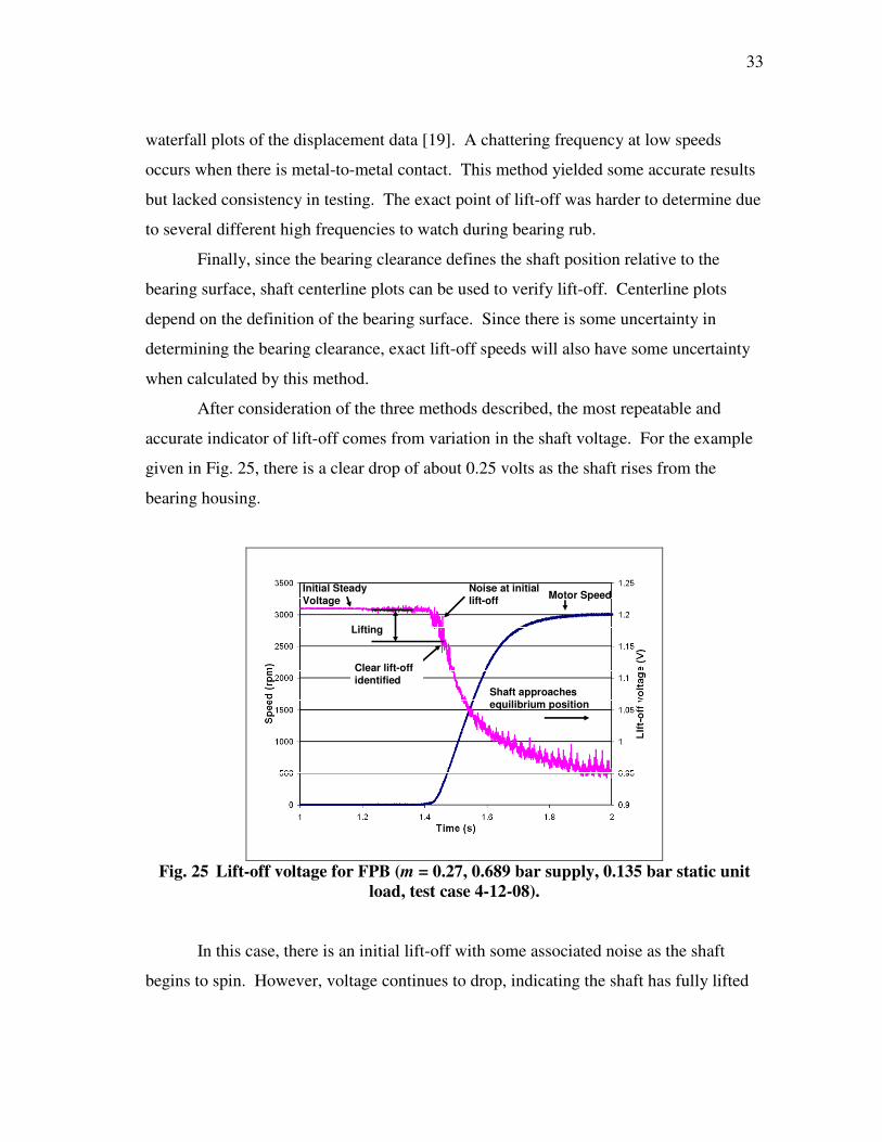
Vibration amplitudes over the range of running speeds can also be used as a

method of verifying lift-off. Accelerometers mounted on the test bearing pedestal record

these vibrations. The amplitudes of these vibrations are plotted in a waterfall plot in Fig.

26 showing the frequency of the vibration and its running speed.

Rubbing frequencies

1X

Note:

EU = m/s2

Fig. 26 Waterfall plot of rubbing frequencies (m = 0.27, 0.689 bar supply, 0.135 bar

static unit load, test case 4-12-08).

The rubbing frequencies are supersynchronous and begin at startup. The

amplitudes of vibrations are significantly reduced by the time the shaft reaches 3000

rpm. However, the rub frequency amplitudes do not all fall off at the same running

35

speed. For example, the vibration closest to the 450 Hz frequency appears to reduce

dramatically near 1500 rpm while the 600 Hz frequency does not drop until 2200 rpm.

This makes it difficult to predict an exact lift-off speed from these data. When the lift-

off voltage technique was used on this same data set, the lift-off speed determined was

460 rpm. This example gives a conflicting result with the lift-off voltage technique,

illustrating the difficulty in achieving consistent results with this method.

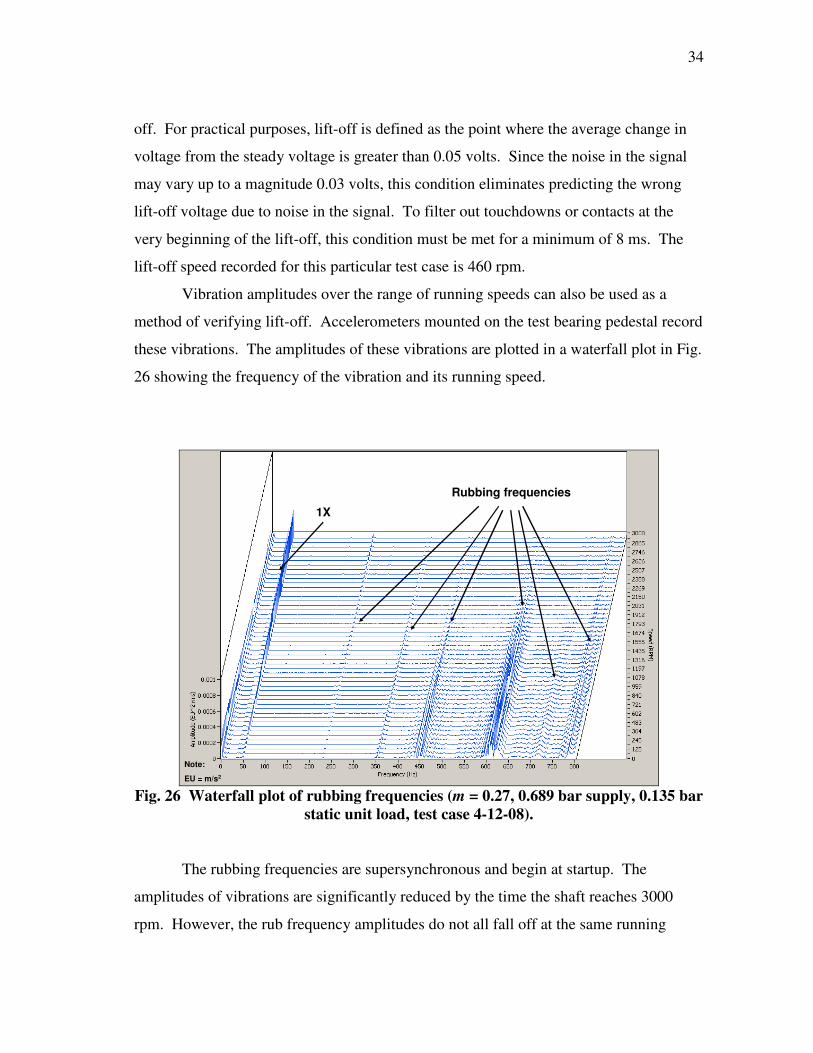
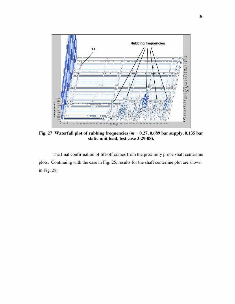
A better case is shown in Fig. 27. The 600 Hz frequency in this test case shows a

drop around 1300 rpm. This is very close to that predicted by the 1380 rpm predicted by

the lift-off voltage technique. The reason for the large difference in lift-off rpm between

this test case and the one done later (4-12-08) can be attributed to a variety of factors.

The m = 0.27 bearing was removed in between the tests and the Cb changed slightly.

Another factor could be some wear at the bearing surface affecting the lift-off speed.

Regardless, this figure is included to show that the rubbing frequency technique does

seem to give an accurate range for the resulting lift-off, but it is difficult to determine an

exact lift-off speed.

36

Rubbing frequencies

1X

Fig. 27 Waterfall plot of rubbing frequencies (m = 0.27, 0.689 bar supply, 0.135 bar

static unit load, test case 3-29-08).

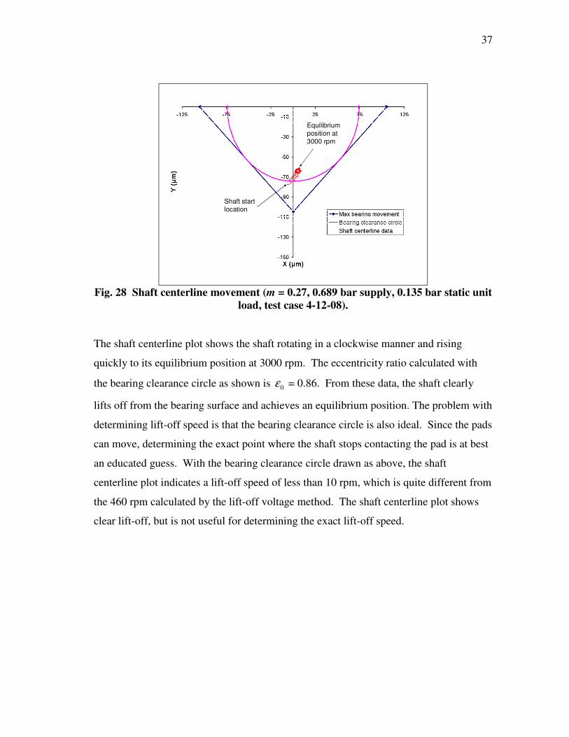
The final confirmation of lift-off comes from the proximity probe shaft centerline

plots. Continuing with the case in Fig. 25, results for the shaft centerline plot are shown

in Fig. 28.

37

Shaft start

location

Equilibrium

position at

3000 rpm

Fig. 28 Shaft centerline movement (m = 0.27, 0.689 bar supply, 0.135 bar static unit

load, test case 4-12-08).

The shaft centerline plot shows the shaft rotating in a clockwise manner and rising

quickly to its equilibrium position at 3000 rpm. The eccentricity ratio calculated with

the bearing clearance circle as shown is 0ε = 0.86. From these data, the shaft clearly

lifts off from the bearing surface and achieves an equilibrium position. The problem with

determining lift-off speed is that the bearing clearance circle is also ideal. Since the pads

can move, determining the exact point where the shaft stops contacting the pad is at best

an educated guess. With the bearing clearance circle drawn as above, the shaft

centerline plot indicates a lift-off speed of less than 10 rpm, which is quite different from

the 460 rpm calculated by the lift-off voltage method. The shaft centerline plot shows

clear lift-off, but is not useful for determining the exact lift-off speed.

38

5. RESULTS

Analyzing test data according to the criteria described in the previous section

enables lift-off speeds to be determined. The lift-off speeds for FPBs will be compared

to results and predictions for a HHB. Recall that predictions are based on the predicted

load capacities of each bearing.

Predictions were made using XLHydrojet®, a rotordynamics program designed

for hydrodynamic and hydrostatic bearings. A grid size of 21 circular points by 13 axial

points was used, and the code was run until it converged. The program does not

calculate lift-off speed directly. Instead, the program predicts eccentricities at specific

running speeds based on an inputted load. Using these eccentricity results and knowing

the bearing clearance allows one to calculate the fluid film thickness via Eq. 7. When

this fluid film thickness falls below 2.0 µm (0.07 mil), which is a typical machined

surface roughness, then contact is assumed to occur. Another way to interpret this same

limit is to say that when the eccentricity ratio is greater than 0.97, contact occurs. The

first speed after the fluid film thickness is greater than the minimum value is the

predicted lift-off speed.

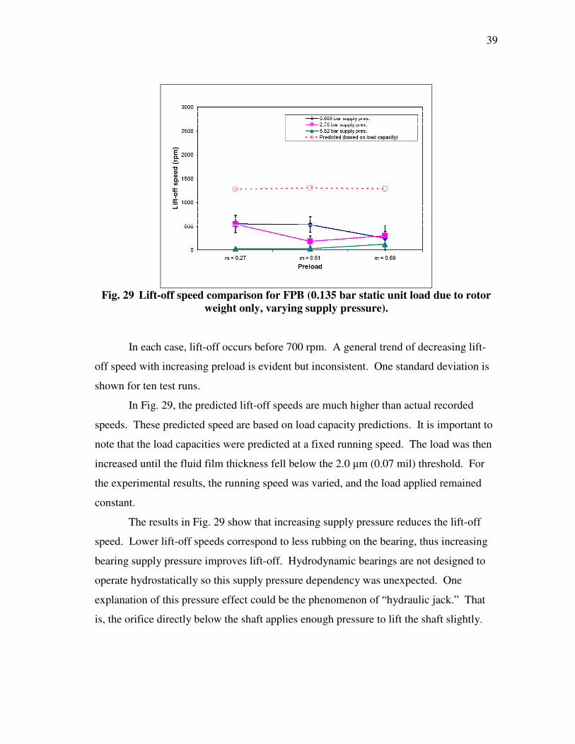
A comparison of the lift-off speeds for the FPBs with a simple constant shaft

weight load (unit load = 0.135 bar) is shown in Fig. 29. No additional load was applied

with the magnetic bearing in this test case.

39

Fig. 29 Lift-off speed comparison for FPB (0.135 bar static unit load due to rotor

weight only, varying supply pressure).

In each case, lift-off occurs before 700 rpm. A general trend of decreasing lift-

off speed with increasing preload is evident but inconsistent. One standard deviation is

shown for ten test runs.

In Fig. 29, the predicted lift-off speeds are much higher than actual recorded

speeds. These predicted speed are based on load capacity predictions. It is important to

note that the load capacities were predicted at a fixed running speed. The load was then

increased until the fluid film thickness fell below the 2.0 µm (0.07 mil) threshold. For

the experimental results, the running speed was varied, and the load applied remained

constant.

The results in Fig. 29 show that increasing supply pressure reduces the lift-off

speed. Lower lift-off speeds correspond to less rubbing on the bearing, thus increasing

bearing supply pressure improves lift-off. Hydrodynamic bearings are not designed to

operate hydrostatically so this supply pressure dependency was unexpected. One

explanation of this pressure effect could be the phenomenon of “hydraulic jack.” That

is, the orifice directly below the shaft applies enough pressure to lift the shaft slightly.

40

This is typically seen in TPBs where the orifice is on the pad. However, this is most

likely not happening in the FPB.

Another explanation comes from the restriction of the flow out of the bearing by

the end seals in the FPB. The end seals prevent the water from exiting immediately,

allowing some pressure development to occur in the “pool” between the pads. The

pressure in this pool helps support the shaft and improve the lift-off in the bearing.

Practically, however, the lowest pressure that still achieves reasonable hydrodynamic

lift-off would be chosen. Hence, for simplicity, the lowest supply pressure of 0.689 bar

will be shown in the following test results. Any exceptions to this are noted in the text.

Linearly Increasing Unit Load

The unit load on each bearing was increased linearly during every test case

except the shaft weight-only cases. That is, the magnetic bearing applied a force that

increased linearly with time. The load started as the shaft began its speed ramp and

reached a maximum at the final running speed, called the design speed. Due to the

nature of the LabView® Virtual Instrument (VI) that sent the force to the bearing, a

force pulse could only be sent once per loop. Thus, loop buffer numbers were selected

to achieve the most force pulses possible. Even so, the result was a fast stepping up of

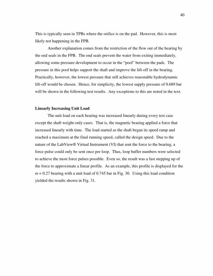
the force to approximate a linear profile. As an example, this profile is displayed for the

m = 0.27 bearing with a unit load of 0.745 bar in Fig. 30. Using this load condition

yielded the results shown in Fig. 31.

41

Force = 0.745 bar at 3000 rpm

Stepping of unit load

Shaft speed

Static shaft weight (0.135 bar)

Fig. 30 Linear unit load force input to system (m = 0.27, 0.745 bar unit load, 0.689

bar supply pressure).

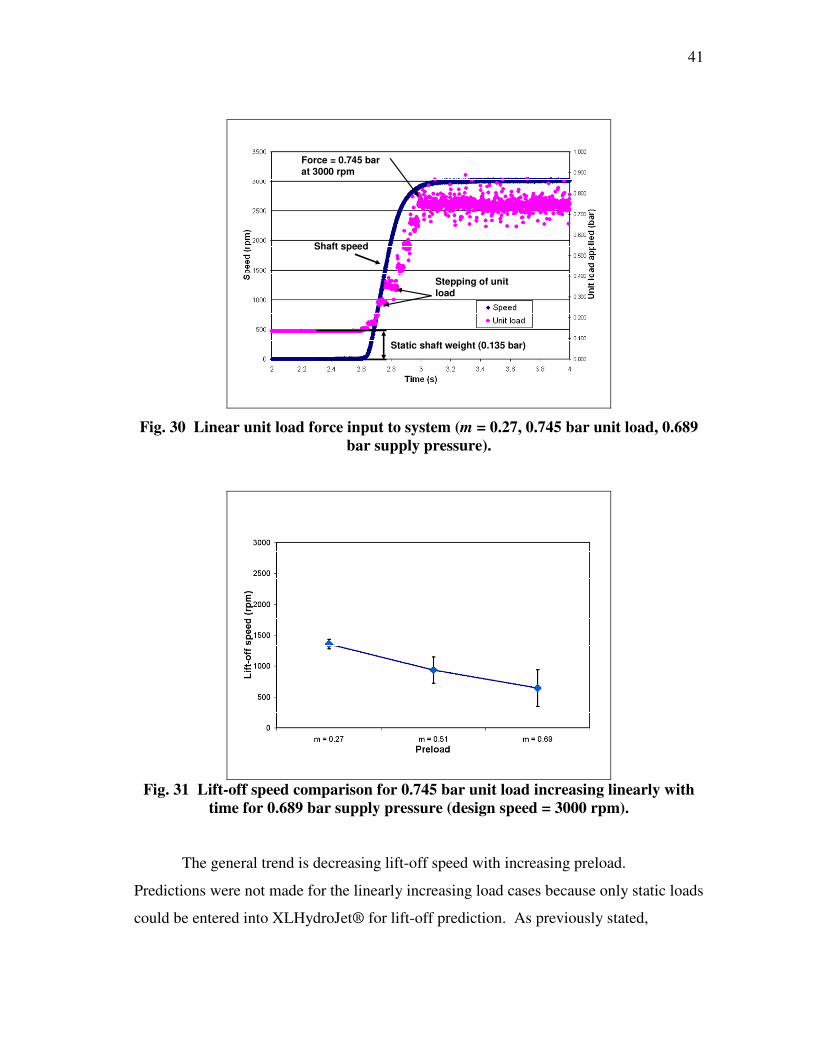
Fig. 31 Lift-off speed comparison for 0.745 bar unit load increasing linearly with

time for 0.689 bar supply pressure (design speed = 3000 rpm).

The general trend is decreasing lift-off speed with increasing preload.

Predictions were not made for the linearly increasing load cases because only static loads

could be entered into XLHydroJet® for lift-off prediction. As previously stated,

42

predictions are based on the load capacity and the code does not give a lift-off speed

result directly.

Lift-off Comparison to HHB

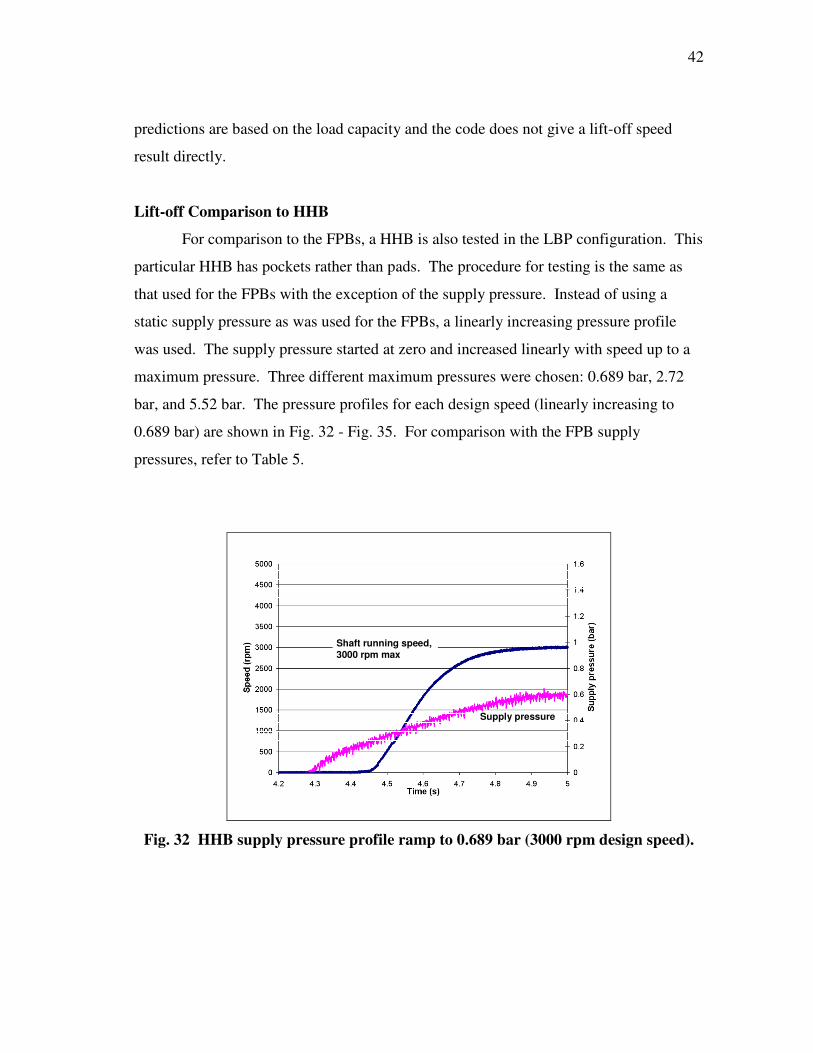
For comparison to the FPBs, a HHB is also tested in the LBP configuration. This

particular HHB has pockets rather than pads. The procedure for testing is the same as

that used for the FPBs with the exception of the supply pressure. Instead of using a

static supply pressure as was used for the FPBs, a linearly increasing pressure profile

was used. The supply pressure started at zero and increased linearly with speed up to a

maximum pressure. Three different maximum pressures were chosen: 0.689 bar, 2.72

bar, and 5.52 bar. The pressure profiles for each design speed (linearly increasing to

0.689 bar) are shown in Fig. 32 - Fig. 35. For comparison with the FPB supply

pressures, refer to Table 5.

Supply pressure

Shaft running speed,

3000 rpm max

Fig. 32 HHB supply pressure profile ramp to 0.689 bar (3000 rpm design speed).

43

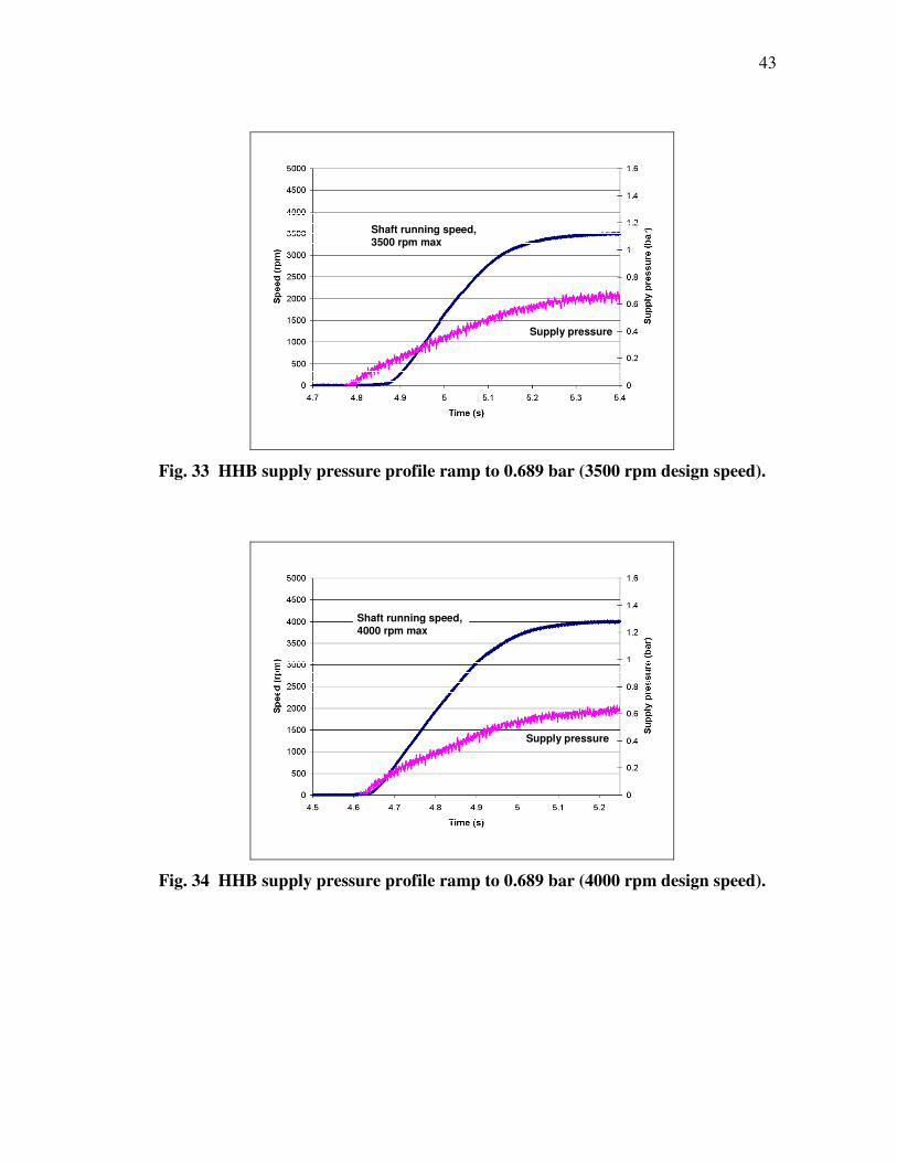
Supply pressure

Shaft running speed,

3500 rpm max

Fig. 33 HHB supply pressure profile ramp to 0.689 bar (3500 rpm design speed).

Supply pressure

Shaft running speed,

4000 rpm max

Fig. 34 HHB supply pressure profile ramp to 0.689 bar (4000 rpm design speed).

44

Supply pressure

Shaft running speed,

4500 rpm max

Fig. 35 HHB supply pressure profile ramp to 0.689 bar (4500 rpm design speed).

With respect to the start of the running speed profile, the pressure profiles did not

start at the same point consistently. Variation in the start time of the pressure profile

would be approximately 0.15 second on either side of the start time of speed profile.

This variation even occurred for the exact same test cases. Since the HHB is pressure

dependent, this greatly influences the results.

Lift-off results are tabulated for the range of running speeds previously

described. The load profiles were adjusted to reach the maximum load at different

design speeds. The design speed is the final running speed of the shaft for a particular

test case. Unfortunately, the motor took different periods of time to reach each design

speed. In fact, it took slightly longer to reach the higher design speeds. That is, there

are different acceleration rates for the same applied unit load.

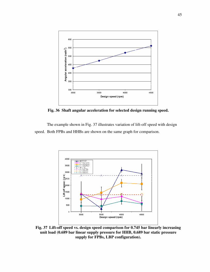
An increasing acceleration with increasing design speed is shown in Fig. 36.

Physically, this means that the bearings with greater acceleration experienced the same

loads at higher running speeds than those with lower accelerations.

45

Fig. 36 Shaft angular acceleration for selected design running speed.

The example shown in Fig. 37 illustrates variation of lift-off speed with design

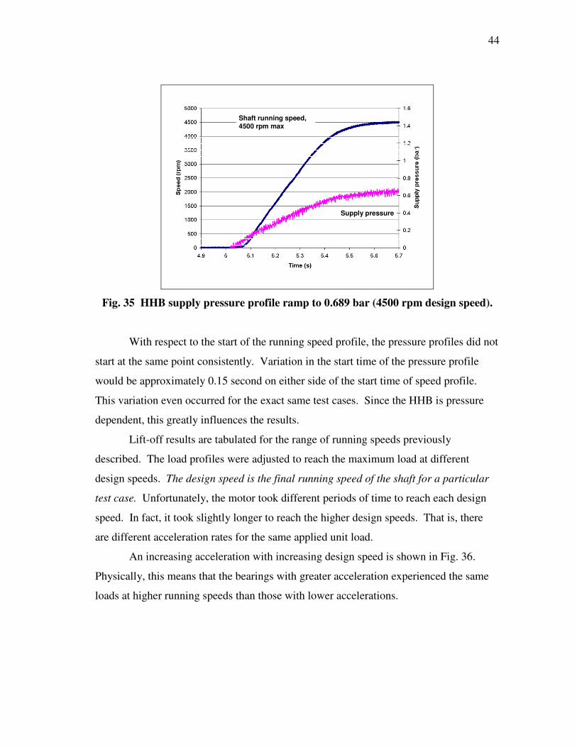
speed. Both FPBs and HHBs are shown on the same graph for comparison.

Fig. 37 Lift-off speed vs. design speed comparison for 0.745 bar linearly increasing

unit load (0.689 bar linear supply pressure for HHB, 0.689 bar static pressure

supply for FPBs, LBP configuration).

46

The results (labeled EXP. in the legend) show no clear trends, and thus no

conclusion can be made about the individual bearings. However, there are large jumps

in the HHB. This graph shows that the HHB is highly pressure dependent. Based on the

previous pressure profile plots, the start time of the pressure ramp severely affects the

lift-off speed in the HHB. As noted in Fig. 32 - Fig. 35, the supply pressure was difficult

to control.

The theoretical lift-off speeds shown in Fig. 37 are based on the load capacity

predictions in XLHydroJet®. The load was increased linearly with time for these test

cases. However, for the predictions, a static maximum load of 0.745 bar was applied,

and the lift-off speed calculated for this load condition.

Since the HHB is pressure dependent, a single pressure profile case and speed

ramp case is chosen for comparison with the FPBs. The shaft weight-only case at 3000

rpm will be used. Since the HHB could only be placed in the bearing housing in the

LOP position, this orientation is compared to the FPB in the LBP position.

Unfortunately, the LBP position was the only available orientation position for the FPB.

LBP tests for the HHB could only be performed by applying an external side load with

the magnetic bearing. The test case for 0.689 bar supply pressure and 0.135 bar unit

load is shown in Fig. 38.

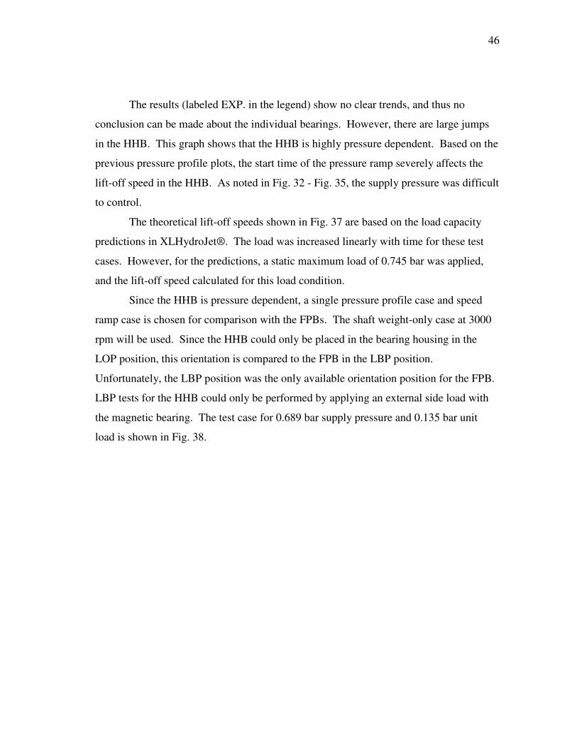
47

Fig. 38 Comparison of FPB vs. HHB for shaft weight-only case (0.135 bar unit

load). LOP at 4500 rpm design speed for HHB and LBP at 3000 rpm design speed

for FPBs. Supply pressure is 0.689 bar linearly increasing for HHB and static

0.689 bar for the FPBs.

When comparing the two types of bearings without load from the magnetic

bearing, it is clear that the FPBs have a much lower lift-off speed. The superior

hydrodynamic ability of the FPBs is evident as it lifts the shaft much earlier than the

HHB does. The predictions for the HHB are very close but the predictions for the FPBs

are more than double the measured results.

Increasing the supply pressure in the HHB yields lift-off results similar to the

FPBs. As shown in Fig. 39, the lift-off speed decreases substantially for an increase in

supply pressure. The predicted lift-off speed is much lower than the speed shown in the

results.

48

Fig. 39 HHB lift-off speed results for increasing supply pressure. (Design speed =

3000 rpm, 0.135 bar static unit load).

Maximum Unit Load Test Results

When the linearly increasing load was applied to the shaft, in most cases the FPB

did not support the maximum load. Instead, the shaft was forced back into contact with

the bearing as illustrated by Fig. 40.

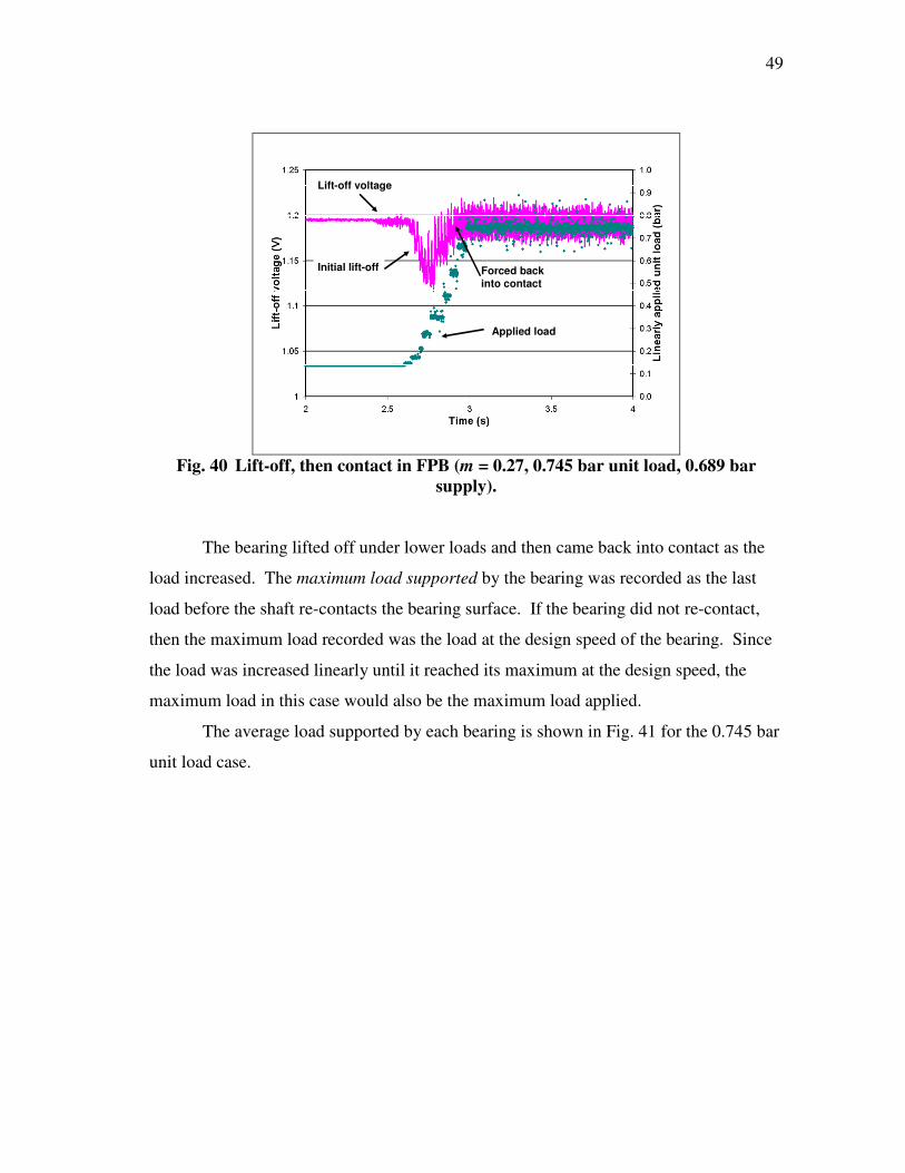
49

Lift-off voltage

Applied load

Initial lift-off Forced back into contact

Fig. 40 Lift-off, then contact in FPB (m = 0.27, 0.745 bar unit load, 0.689 bar

supply).

The bearing lifted off under lower loads and then came back into contact as the

load increased. The maximum load supported by the bearing was recorded as the last

load before the shaft re-contacts the bearing surface. If the bearing did not re-contact,

then the maximum load recorded was the load at the design speed of the bearing. Since

the load was increased linearly until it reached its maximum at the design speed, the

maximum load in this case would also be the maximum load applied.

The average load supported by each bearing is shown in Fig. 41 for the 0.745 bar

unit load case.

50

Fig. 41 Maximum unit load supported for various preloads in FPBs (0.745 bar

linearly increasing unit load at 0.689 bar supply pressure, design speed = 3000

rpm).

Generally, the m = 0.27 bearing shows the highest load capacity, while the m =

0.69 bearing showed a slightly lower load capacity. The m = 0.51 bearing did not

support any load at this supply pressure. It did support load at higher supply pressures,

but it still had the worst load capacity of all three FPBs. A figure showing results for all

the supply pressures is provided in the Appendix.

Comparing the FBP to the HHB at the 0.689 bar supply pressure proved difficult.

The HHB did not lift-off until higher running speeds, so the chart in Fig. 42 compares

the bearings at a design speed of 4500 rpm.

51

Fig. 42 Comparison of FPB and HHB maximum supported unit load for design

speed = 4500 rpm, 0.689 bar supply pressure (static for FPB, linearly increasing for

HHB), LBP configuration, 1.380 bar linearly applied unit load.

The results indicate that the HHB supports at least twice the load that the FPBs

do. The maximum applied load in this case is 1.380 bar, and this is supported by the

HHB. The load capacity of the HHB is superior to that of the FPBs.

Eccentricity Ratios

The only load profile where final eccentricities were obtained for the FPBs was

for the 0.135 bar static unit loading case. The other cases loaded the shaft so that it

remained in contact with the bearing. Since the shaft can rub outside of the Cb with the

movement of the pads, this resulted in calculated eccentricities greater than one. The

0.135 bar static unit load case gave eccentricity ratios at 3000 rpm as shown in Fig. 43.

52

Fig. 43 Final eccentricity ratios for 0.135 bar unit load at 3000 rpm, 0.689 bar

pressure supply in a FPB.

The lower the eccentricity ratio, the closer the shaft is to the bearing center. High

eccentricities operate near the bearing surface and are more prone to rub. The

predictions show a decreasing eccentricity ratio with increasing preload. This matches

the trend found in the FPB results for the m = 0.27 and m = 0.51 case but is in conflict

with the m = 0.69 results.

The results for the HHB compared to the FPBs at a linearly increasing 0.689 bar

supply pressure are shown in Fig. 44.

53

Fig. 44 Comparison of HHB and FPB at 3000 rpm, shaft weight-only case (0.135

bar unit load). Supply pressure is static at 0.689 bar for FPBs and linearly

increasing to 0.689 bar for the HHB. Orientation is LBP for FPBs and LOP for

HHB.

The HHB has much lower eccentricities than the FPB for the shaft weight-only

case. Due to the bolthole arrangement in the bearing housing, the orientations of LBP

for FPBs and LOP for HHB were the only ones possible when considering the shaft

weight-only case. Future experiments should orient the shaft weight directly between

the pockets for the HHB to confirm that its eccentricity ratio is still lower than the

FPBs’.

Attitude Angle

The attitude angle indicates the position of the shaft with respect to the load. For

the FPBs, the load was applied downward in the vertical direction. Due to the

orientation of the HHB, however, the load was applied as a horizontal side load to

achieve a load-between-pocket configuration instead of a load-on-pocket. During

experiments, the attitude angle did not vary with supply pressure significantly for the

FPBs. Thus, the 3000 rpm, 0.689 bar supply pressure is chosen for results shown in Fig.

54

45. These results show the LOP configuration of the HHB since that was the only

configuration available for the shaft weight-only case.

Fig. 45 Attitude angle comparison for HHB (LOP) and m = 0.51 (LBP) for 3000

rpm and 0.689 bar supply pressure.

Attitude angles are slightly lower for the FPB than the HHB. In comparison to

the predictions for the 0.135 bar unit load case, results are much lower than the predicted

attitude angle. The simulations showed the shaft moving in the horizontal direction for

light loads, which is indicative of no cavitation. Increasing the unit load to 0.745 bar

achieves predicted attitude angles closer to the experimental results.

The predictions for the HHB do vary with supply pressure, which is consistent

with the experimental results for higher load cases. A very good match between

predicted (TH.) and experimental (EXP.) results is confirmed in Fig. 46. The shaft was

placed under a side load in order to maintain a LBP configuration. Hence, lower loads

were not available for the LBP configuration.

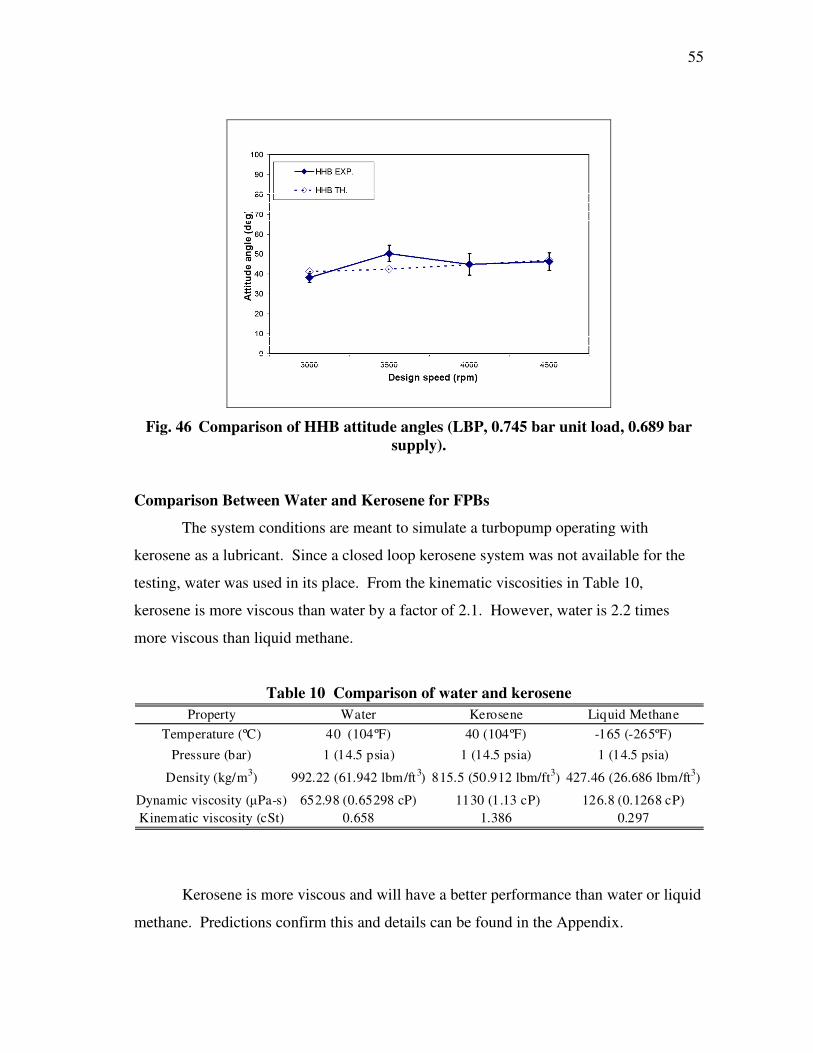
55

Fig. 46 Comparison of HHB attitude angles (LBP, 0.745 bar unit load, 0.689 bar

supply).

Comparison Between Water and Kerosene for FPBs

The system conditions are meant to simulate a turbopump operating with

kerosene as a lubricant. Since a closed loop kerosene system was not available for the

testing, water was used in its place. From the kinematic viscosities in Table 10,

kerosene is more viscous than water by a factor of 2.1. However, water is 2.2 times

more viscous than liquid methane.

Table 10 Comparison of water and kerosene

Property Water Kerosene Liquid Methane

Temperature (ºC) 40 (104ºF) 40 (104ºF) -165 (-265ºF)

Pressure (bar) 1 (14.5 psia) 1 (14.5 psia) 1 (14.5 psia)

Density (kg/m3) 992.22 (61.942 lbm/ft

3) 815.5 (50.912 lbm/ft

3) 427.46 (26.686 lbm/ft

3)

Dynamic viscosity (µPa-s) 652.98 (0.65298 cP) 1130 (1.13 cP) 126.8 (0.1268 cP)

Kinematic viscosity (cSt) 0.658 1.386 0.297

Kerosene is more viscous and will have a better performance than water or liquid

methane. Predictions confirm this and details can be found in the Appendix.

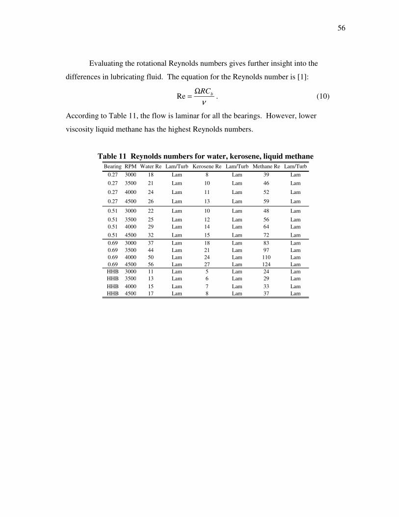
56

Evaluating the rotational Reynolds numbers gives further insight into the

differences in lubricating fluid. The equation for the Reynolds number is [1]:

νbRCΩ

=Re . (10)

According to Table 11, the flow is laminar for all the bearings. However, lower

viscosity liquid methane has the highest Reynolds numbers.

Table 11 Reynolds numbers for water, kerosene, liquid methane

Bearing RPM Water Re Lam/Turb Kerosene Re Lam/Turb Methane Re Lam/Turb

0.27 3000 18 Lam 8 Lam 39 Lam

0.27 3500 21 Lam 10 Lam 46 Lam

0.27 4000 24 Lam 11 Lam 52 Lam

0.27 4500 26 Lam 13 Lam 59 Lam

0.51 3000 22 Lam 10 Lam 48 Lam

0.51 3500 25 Lam 12 Lam 56 Lam

0.51 4000 29 Lam 14 Lam 64 Lam

0.51 4500 32 Lam 15 Lam 72 Lam

0.69 3000 37 Lam 18 Lam 83 Lam

0.69 3500 44 Lam 21 Lam 97 Lam

0.69 4000 50 Lam 24 Lam 110 Lam

0.69 4500 56 Lam 27 Lam 124 Lam

HHB 3000 11 Lam 5 Lam 24 Lam

HHB 3500 13 Lam 6 Lam 29 Lam

HHB 4000 15 Lam 7 Lam 33 Lam

HHB 4500 17 Lam 8 Lam 37 Lam

57

6. SUMMARY

Several different methods for detection of lift-off speeds were performed in these

experiments. The most basic method is to evaluate the shaft centerline plots and view

the upward motion of the shaft. A measured bearing clearance is required to determine

the lift-off speed. The main problem with this method is that there can be uncertainties

not only in the motion of the shaft but also in the measured bearing clearance.

The next method, which proved more reliable, was to look at the vibration

frequencies of the bearing housing as the shaft accelerates. Accelerometers on the

bearing housing showed supersynchronous frequencies that dropped off as the shaft

lifted upwards. When comparing these frequencies to running speed, it was difficult to

ascertain the exact speed of lift-off. Several high-level frequencies developed but did

not all drop off at the same time consistently.

The final method and the one selected for determination of lift-off speed, was to

measure the voltage across a resistor in a shaft circuit. When the shaft lifted off, the

voltage drop across the resistor was significant enough to give a consistent lift-off speed

measurement. Problems with this method include noise in the shaft circuit and

assumptions as to when to consider the shaft fully lifted off. Since the shaft may initially

lift up slightly then fall back in contact, the exact lift-off point was defined to be the

point where the voltage dropped 0.05 volts from the mean value for at least 8 ms. This

point was chosen as a conservative estimate to yield consistent results regardless of the

noise in the signal. Future experiments may wish to refine these assumptions.

58

7. CONCLUSIONS

In comparison to load-capacity-based predictions for FPBs, the experimental

results showed lower lift-off speeds, higher load capacities, higher eccentricity ratios,

and lower attitude angles. Load capacity does appear to affect lift-off speed but no clear

trend was found. Hence, lift-off speed is poorly predicted from load capacity.

Some factors that future experiments need to consider are pressure dependency

and design speed. The design speed is the maximum running speed achieved for a

particular test run. The FPBs unexpectedly proved to be highly pressure dependent due

to an end-seal phenomenon. Since the HHB is also pressure dependent, changing design

speeds with linearly increasing force and pressure profiles was difficult to perform

consistently. In these experiments, increasing design speed also increased the

acceleration of the shaft.

Another difficultly arose in the form of orientation. Due to the design of the

bearing housing, the HHB could only be placed in the LOP position and the FPB in the

LBP position. External loads were applied to the shaft for the HHB test cases to

compare the LBP positions for both bearings.

The HHB showed greater load capacity and lower eccentricities than the FPBs,

but the FPBs had lower lift-off speeds and attitude angles. This comparison is for a

0.689 bar supply pressure and 3000 rpm design speed. At this supply pressure and

considering the shaft weight-only case, the FPB in the LBP orientation had much lower

lift-off speeds than the HHB in the LOP orientation. Increasing the supply pressure to

the HHB decreased its lift-off speed to much lower levels. Hence, for lower supply

pressures, the FPB outperformed the HHB in terms of lift-off speed. If the load capacity

needed in the bearing application remains relatively small, a FPB could replace an HHB.

59

REFERENCES

[1] San Andrés, L., 2006, “Modern Hydrodynamic Lubrication Theory,” Texas A&M

University MEEN 626 Class Notes. http://phn.tamu.edu/me626. Access date: May

2007.

[2] Childs, D. and Al-Ghasem, A., 2006, “Rotordynamic Coefficients Measurements

Versus Predictions for a High-Speed Flexure-Pivot Tilting-Pad Bearing (Load-

Between-Pad Configuration),” J. Eng. Gas Turb. Power, 128, pp. 896-906.

[3] Chen, W. J., 1995, “Bearing Dynamic Coefficient of Flexible Pad Bearings,”

Tribol. T., 38(2), pp. 253-260.

[4] Childs, D., 1993, “Turbomachinery Rotordynamics: Phenomena, Modeling, and

Analysis,” John Wiley, New York.

[5] Kepple, W. E., Read, D. W., Zeidan, F. Y., Paraskevakos, C., and Dawson, M. P.,

1998, "Experience in the Use of Flexure Pivot Tilt Pad Bearings in Boiler Feed

Water Pumps," Proceedings of the 15th International Pump Users Symposium,

Turbomachinery Laboratory, College Station, TX, pp. 77-84.

[6] Rodriguez, L., 2004, “Experimental Frequency-Dependent Rotordynamic

Coefficients for a Load-On-Pad, High-Speed, Flexible-Pivot Tilting-Pad Bearing,”

M.S. thesis, Texas A&M University, College Station, Texas.

[7] Zeidan, F., 1992, “Developments in Fluid Film Bearing Technology,” Turbomach.

Int., 9, pp. 24-31.

[8] San Andrés, L., 1996, “Turbulent Flow, Flexure-Pivot Hybrid Bearings for

Cryogenic Applications,” ASME J. Tribol., 118(1), pp. 190-200.

[9] “XLTRC2: Rotordynamics Software Suite,” The Turbomachinery Laboratory,

Texas A&M University.

http://turbolab.tamu.edu/research/trc/XLTRC%202002.pdf. Access date: August

2008.

[10] “XLHYDROJET: Computational Analyses of Hydrostatic/Hydrodynamic

Bearings,” Texas A&M University.

http://phn.tamu.edu/TRIBGroup/Soft_hydrojet_1.htm. Access date: August 2008.

60

[11] Zeidan, F. and Paquette, D., 1994, “Application of High Speed and Higher

Performance Fluid Film Bearings in Rotation Machinery,” Proceedings of the 23rd

Turbomachinery Symposium, Turbomachinery Laboratory, Texas A&M

University, Dallas, TX, pp. 209-234.

[12] De Choudhury, P., Hill, M., and Paquette, D., 1992, “A Flexible Pad Bearing

System for a High Speed Centrifugal Compressor,” Proceedings of the 21st

Turbomachinery Symposium, Turbomachinery Laboratory, Texas A&M

University, Dallas, TX, pp. 57-64.

[13] Armentrout, R., and Paquette, D., 1993, “Rotordynamic Characteristics of Flexure-

Pivot Tilting-Pad Journal Bearings,” Tribol. T., 36(3), pp. 443-451.

[14] Elwell, R. C., and Findlay, J. A., 1969, “Design of Pivoted-Pad Journal Bearings,”

ASME J. Lubric. Tech., 91(1), pp. 87–103.

[15] Wygant, K., Flack, R., and Barrett, L., 2004, “Measured Performance of Tilting-

Pad Journal Bearings over a Range of Preloads—Part 1: Static Operating

Conditions,” Tribol. T., 47, pp. 576-584.

[16] Scharrer, J.K., Tellier, J.G., and Hibbs, R.I., 1991, “A Study of the Transient

Performance of Hydrostatic Journal Bearings: Part II-Experimental Results,”

STLE/ASME Tribology Conference, STLE Paper 91-TC-3B-2, St. Louis, MO, pp.

1-7.

[17] Zhu, X., 2004, “Experimental Response of a Rotor Supported on Rayleigh Step

Bearings,” M.S. thesis, Texas A&M University, College Station, TX.

[18] Lu, X. and Khonsari, M. 2005, “On the Lift-off Speed in Journal Bearings,”

Tribol. Lett., 20, pp. 299-305.

[19] Bouyer, J., Fillon, M., and Pierre-Danos, I., 2006, “Influence of Wear on the

Behavior of a Two-lobe Hydrodynamic Journal Bearing Subjected to Numerous

Start-ups and Stops,” Proceedings of IJTC2006 STLE/ASME International Joint

Tribology Conference, San Antonio, TX.

61

[20] ASME B46.1-2002 Surface Texture (Surface Roughness, Waviness, and Lay),

American Society of Mechanical Engineers (ASME), New York.

[21] Dyck, B.J., 2007. “Experimental Study of Dry-friction Whirl and Whip for a

Rotor Supported by an Annular Rub Surface,” Master’s report, Texas A&M

University, College Station, TX.

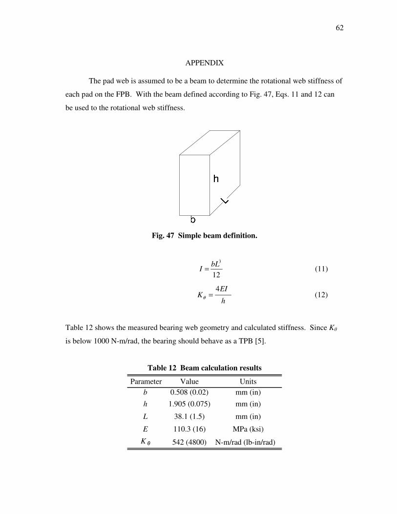
62

APPENDIX

The pad web is assumed to be a beam to determine the rotational web stiffness of

each pad on the FPB. With the beam defined according to Fig. 47, Eqs. 11 and 12 can

be used to the rotational web stiffness.

Fig. 47 Simple beam definition.

12

3bL

I = (11)

h

EIK

4=θ (12)

Table 12 shows the measured bearing web geometry and calculated stiffness. Since Kθ

is below 1000 N-m/rad, the bearing should behave as a TPB [5].

Table 12 Beam calculation results

Parameter Value Units

b 0.508 (0.02) mm (in)

h 1.905 (0.075) mm (in)

L 38.1 (1.5) mm (in)

E 110.3 (16) MPa (ksi)

K θ 542 (4800) N-m/rad (lb-in/rad)

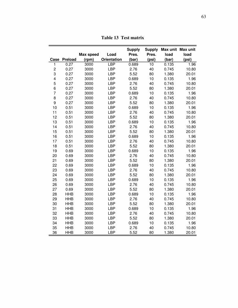
63

Table 13 Test matrix

Case Preload

Max speed

(rpm)

Load

Orientation

Supply

Pres.

(bar)

Supply

Pres.

(psi)

Max unit

load

(bar)

Max unit

load

(psi)

1 0.27 3000 LBP 0.689 10 0.135 1.96

2 0.27 3000 LBP 2.76 40 0.745 10.80

3 0.27 3000 LBP 5.52 80 1.380 20.01

4 0.27 3000 LBP 0.689 10 0.135 1.96

5 0.27 3000 LBP 2.76 40 0.745 10.80

6 0.27 3000 LBP 5.52 80 1.380 20.01

7 0.27 3000 LBP 0.689 10 0.135 1.96

8 0.27 3000 LBP 2.76 40 0.745 10.80

9 0.27 3000 LBP 5.52 80 1.380 20.01

10 0.51 3000 LBP 0.689 10 0.135 1.96

11 0.51 3000 LBP 2.76 40 0.745 10.80

12 0.51 3000 LBP 5.52 80 1.380 20.01

13 0.51 3000 LBP 0.689 10 0.135 1.96

14 0.51 3000 LBP 2.76 40 0.745 10.80

15 0.51 3000 LBP 5.52 80 1.380 20.01

16 0.51 3000 LBP 0.689 10 0.135 1.96

17 0.51 3000 LBP 2.76 40 0.745 10.80

18 0.51 3000 LBP 5.52 80 1.380 20.01

19 0.69 3000 LBP 0.689 10 0.135 1.96

20 0.69 3000 LBP 2.76 40 0.745 10.80

21 0.69 3000 LBP 5.52 80 1.380 20.01

22 0.69 3000 LBP 0.689 10 0.135 1.96

23 0.69 3000 LBP 2.76 40 0.745 10.80

24 0.69 3000 LBP 5.52 80 1.380 20.01

25 0.69 3000 LBP 0.689 10 0.135 1.96

26 0.69 3000 LBP 2.76 40 0.745 10.80

27 0.69 3000 LBP 5.52 80 1.380 20.01

28 HHB 3000 LBP 0.689 10 0.135 1.96

29 HHB 3000 LBP 2.76 40 0.745 10.80

30 HHB 3000 LBP 5.52 80 1.380 20.01

31 HHB 3000 LBP 0.689 10 0.135 1.96

32 HHB 3000 LBP 2.76 40 0.745 10.80

33 HHB 3000 LBP 5.52 80 1.380 20.01

34 HHB 3000 LBP 0.689 10 0.135 1.96

35 HHB 3000 LBP 2.76 40 0.745 10.80

36 HHB 3000 LBP 5.52 80 1.380 20.01

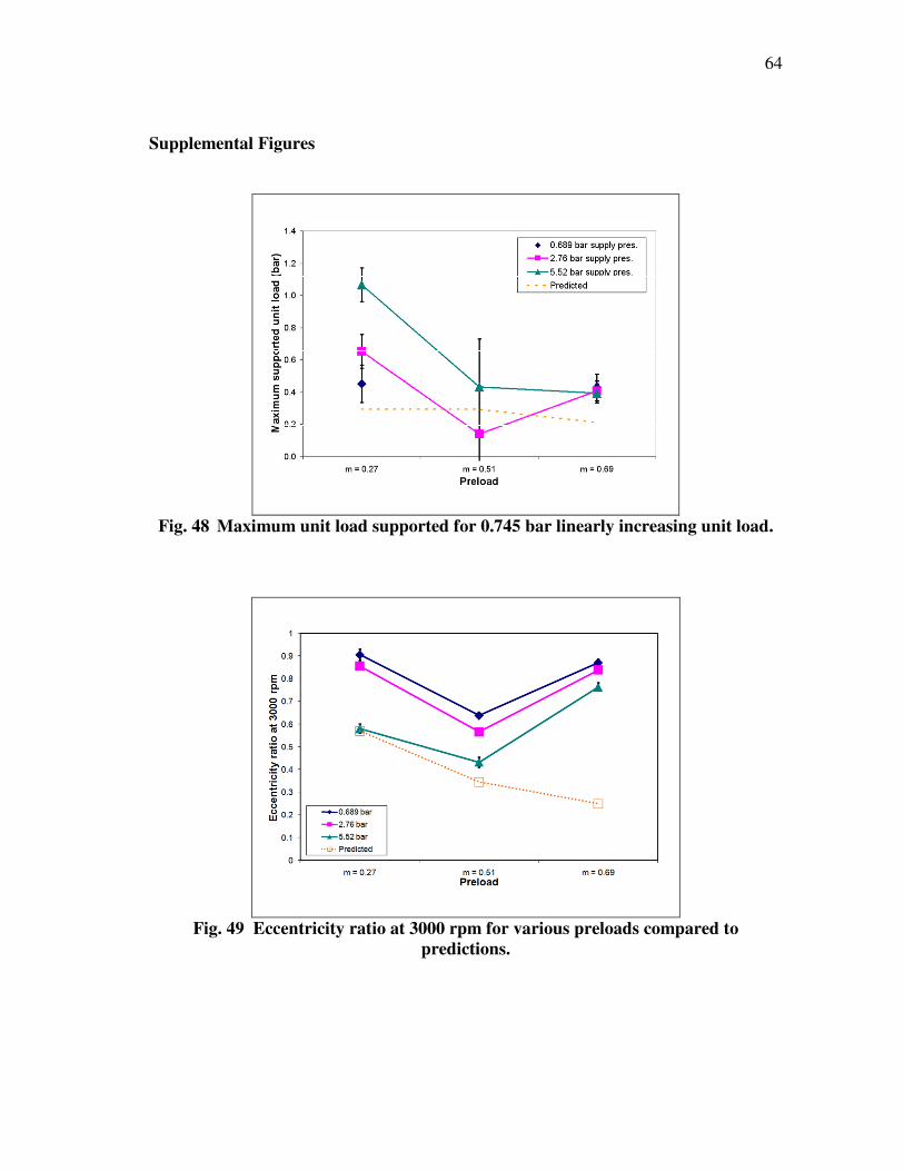
64

Supplemental Figures

Fig. 48 Maximum unit load supported for 0.745 bar linearly increasing unit load.

Fig. 49 Eccentricity ratio at 3000 rpm for various preloads compared to

predictions.

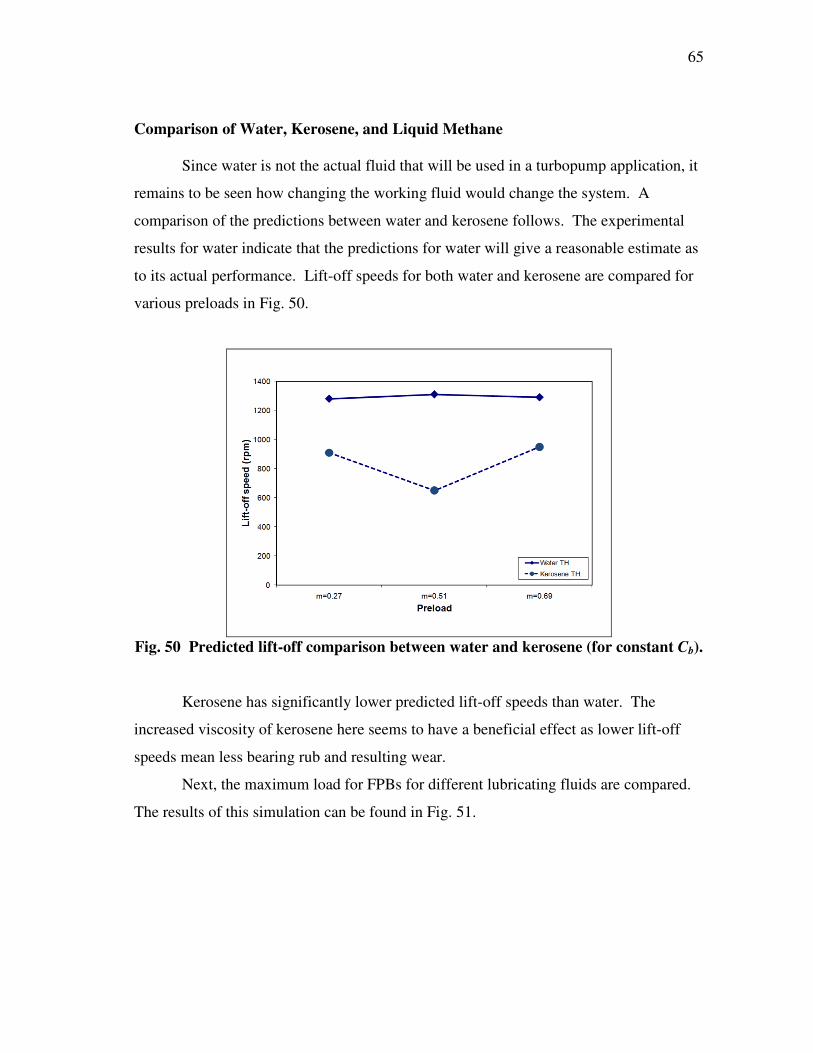
65

Comparison of Water, Kerosene, and Liquid Methane

Since water is not the actual fluid that will be used in a turbopump application, it

remains to be seen how changing the working fluid would change the system. A

comparison of the predictions between water and kerosene follows. The experimental

results for water indicate that the predictions for water will give a reasonable estimate as

to its actual performance. Lift-off speeds for both water and kerosene are compared for

various preloads in Fig. 50.

Fig. 50 Predicted lift-off comparison between water and kerosene (for constant Cb).

Kerosene has significantly lower predicted lift-off speeds than water. The

increased viscosity of kerosene here seems to have a beneficial effect as lower lift-off

speeds mean less bearing rub and resulting wear.

Next, the maximum load for FPBs for different lubricating fluids are compared.

The results of this simulation can be found in Fig. 51.

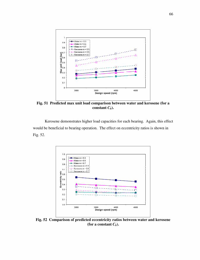
66

Fig. 51 Predicted max unit load comparison between water and kerosene (for a

constant Cb).

Kerosene demonstrates higher load capacities for each bearing. Again, this effect

would be beneficial to bearing operation. The effect on eccentricity ratios is shown in

Fig. 52.

Fig. 52 Comparison of predicted eccentricity ratios between water and kerosene

(for a constant Cb).

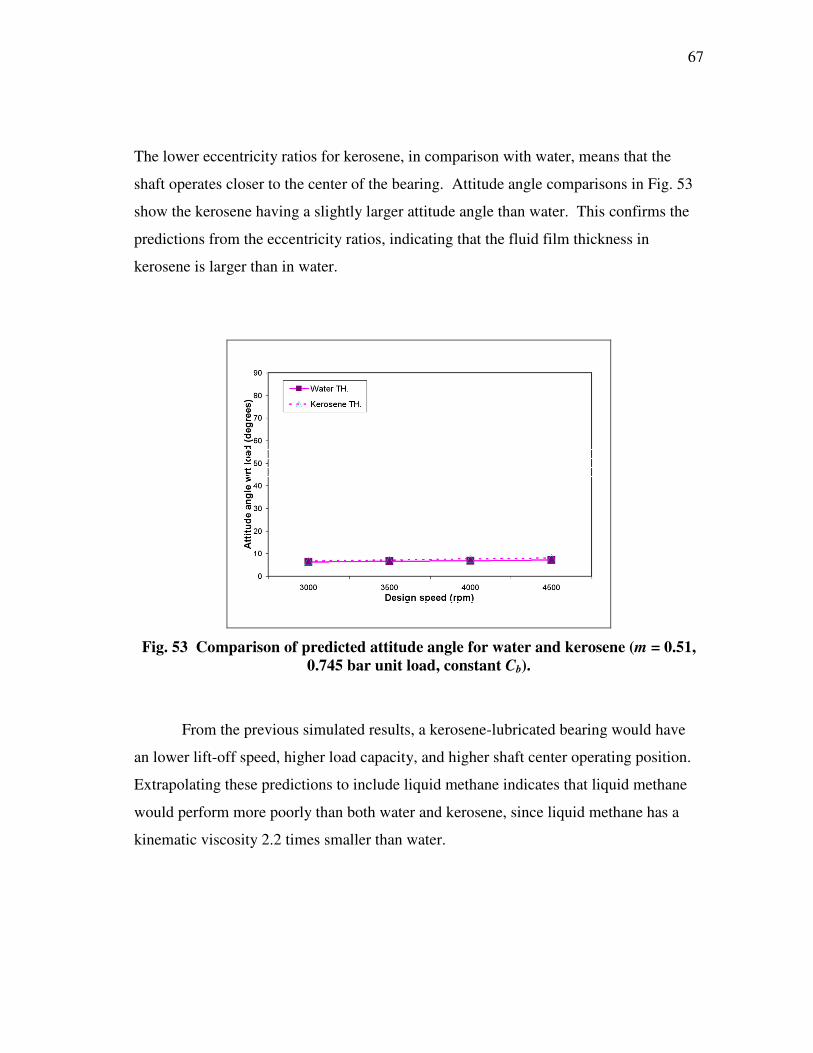
67

The lower eccentricity ratios for kerosene, in comparison with water, means that the

shaft operates closer to the center of the bearing. Attitude angle comparisons in Fig. 53

show the kerosene having a slightly larger attitude angle than water. This confirms the

predictions from the eccentricity ratios, indicating that the fluid film thickness in

kerosene is larger than in water.

Fig. 53 Comparison of predicted attitude angle for water and kerosene (m = 0.51,

0.745 bar unit load, constant Cb).

From the previous simulated results, a kerosene-lubricated bearing would have

an lower lift-off speed, higher load capacity, and higher shaft center operating position.

Extrapolating these predictions to include liquid methane indicates that liquid methane

would perform more poorly than both water and kerosene, since liquid methane has a

kinematic viscosity 2.2 times smaller than water.

68

VITA

David Hunter Mertz

Department of Mechanical Engineering

3123 TAMU

College Station TX 77843-3123

david.h.mertz@gmail.com

Education:

M.S. Mechanical Engineering

December 2008

Texas A&M University

B.S. Engineering Science ’06

Trinity University - San Antonio, TX

Work Experience:

Mechanical Engineer, Siemens Energy, Inc., Houston, TX

• Design of systems for gas turbines and compressors

• Conducted structural design analysis using FEA modeling in ANSYS

• Simulated process flows with HYSYS for oil and gas applications

Research Assistant, Texas A&M Turbomachinery Laboratory, College Station, TX

• Designed a flexure pivot pad bearing for lift-off testing

• Conducted rotordynamic tests on hybrid bearing designs for use in rocket engine

turbopumps

• Installed and instrumented a water control valve for use in turbomachinery

applications

Intern, American National Power, Midlothian, TX

• Designed a parking lot in AutoCAD while maintaining compliance with ADA code

• Implemented a safety relief valve inspection program in compliance with ASME

code

• Studied aspects of the design of a combined cycle power plant