Papercrete Thermal Test Report (includes R-Value)

1 Introduction

The thermal conductivity is one of the fundamental properties of a material and it

is governed by the Fourier’s Law:

Q = k ·A· ΔT / L

where,

Q = Heat transfer

A = Area of the specimen (Figure 1)

L = Thickness of the specimen

k = Thermal conductivity, and

ΔT = Difference in temperature between two sections (of area A) at a distance L.

(ΔT = T1-T0)

FIG. 1. Heat Flow

The heat transfer can be written as:

1

Q = U·A· ΔT

where U = K / L is the conductance.

The thermal resistance (R) is defined as the inverse of the conductance:

R = 1 / U

and it is used as a measure of the thermal insulation capacity of a material.

In the Customary System of Units (English), the resistance is measured in [Btu/

(hr·ft²·°F)]. Btu is the heat required to warm one pound of water through the interval of

1°F.

In the International System of Units (SI), it is measured in [W/(m²·°C)]. The

conversion factor is 0.1761 [i.e. 1 Btu/(hr·ft²·°F) ≈ 0.1761 W/(m²·°C)].

2 Test Procedure

The measurement of the parameters that are necessary to calculate the thermal

conductivity is based on the Standard Method for Thermal Conductivity (Ashraful 2005).

This experimental method was developed for paving materials and it employs a steady

one dimensional conduction approach. A brief summary of this method is presented.

• Thermocouples (temperature sensors) are placed on top, bottom and sides of

the cylindrical sample of 75 mm diameter and 100 mm height as it is shown in

Figures 2 and 3.

2

FIG. 2. Dimensions of Cylindrical Sample for Thermal Conductivity Test

FIG. 3. Temperature Sensor Setup in the Specimens.

3

Three sensors were attached on the top section and three on the bottom of the

sample in order to obtain the temperature difference (ΔT). Sensors were also

placed on the lateral contour of the sample to compute the heat loss.

• Two thermocouples were attached to the hotplate (see Figure 4).The

papercrete sample was insulated by a Styrofoam box with the top face of the

sample exposed (see Figure 5). The assembly shown in Figure 5 was placed into

the environmental chamber that is used to keep constant temperature during the

test.

FIG. 4. Hot Plate Setup

Three temperature sensors were placed in the surrounding Styrofoam and two

sensors below the hot plate in order to compute heat loss.

4

FIG. 5. Thermal Conductivity Test

• The thermocouples were connected to the data acquisition system (see Figure 6)

which is a device that allows registering the temperature in °C from all sensors in

a data file. Temperature data were taken every 30 seconds.

5

FIG. 6. Connection of Temperature Sensors to the Data Acquisition System

• The hot plate is powered by a DC current supply set to 5 volts and 0.74 amperes

which heats the hot plate at about 60 °C until a steady state difference (ΔT)

between the bottom and the top of the sample is achieved. The steady state is

achieved when the temperatures become constant with time; that is the

temperature curves become flat. The heat flow (Q) then is also constant with time.

This may be seen on the computer screen by noting that the temperature data do

not experiment significant changes or by checking if the Temperature vs Time

curves corresponding to the top and the bottom have become flat (see Figure 7).

6

0

10

20

30

40

50

60

70

0 50 100 150 200 250 300Time (min)

Temp (C) PapercreteSample 4

Top

Bottom

ΔT

FIG. 7. Temperature Steady State

3 Results

Five papercrete samples and one Styrofoam sample were subjected to a heat

source in order to study the ability of the material to conduct heat. The Styrofoam sample

was used to calibrate the results. The R value for the Styrofoam is known, equals to 4 per

inch. A Temperature vs Time curve was developed for each sample so that the

7

temperature difference (ΔT) may be obtained under a steady state condition (constant

temperature at the bottom and at the top of the sample). Average temperatures of sensors

placed at the same location were used for all calculations. Table 1 presents the results for

the thermal conductivity test as well as the R values for each sample.

Table 1. Thermal Conductivity (k) and R values

No Sample k(W/(m °C)

Corrected k (W/(m °C))

RSI value per inch(m²·°C/W)

R value per inch (Btu/(hr·ft²·°F))

1 1 0.40 0.04974 0.51 2.92 3 0.44 0.05471 0.46 2.63 4 0.38 0.04725 0.54 3.14 59a 0.38 0.04725 0.54 3.15 59b 0.36 0.04476 0.57 3.2

The “Corrected k” value was calibrated based on a known value of k = 0.03606 W/(m°C)

for the Styrofoam used. All calculations as well as all Temperature vs Time graphs for

each sample may be found in Appendix IV.

4 Conclusions and Recommendations

• Based on the results of the R values obtained, it is apparent that papercrete is a

good insulator. Papercrete R values range from about 2.6 to 3.2 per inch (Table

1). For a wall about 1 foot thick, the R value should be somewhat more than 30.

8

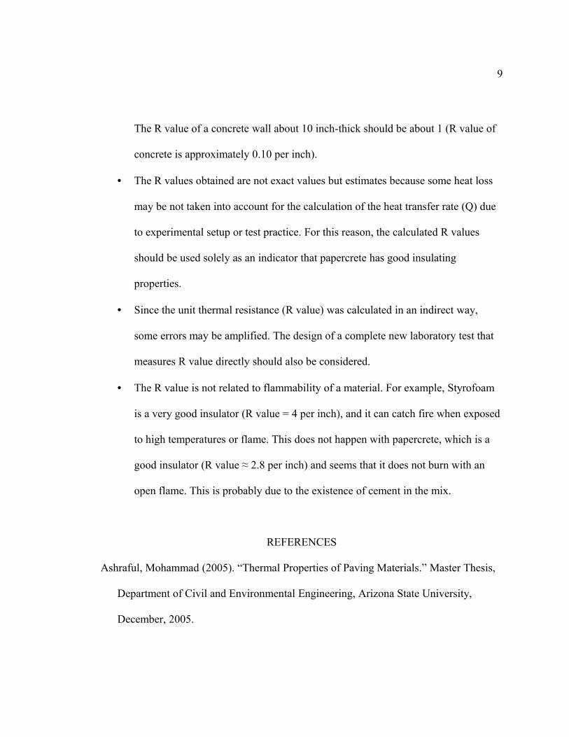
The R value of a concrete wall about 10 inch-thick should be about 1 (R value of

concrete is approximately 0.10 per inch).

• The R values obtained are not exact values but estimates because some heat loss

may be not taken into account for the calculation of the heat transfer rate (Q) due

to experimental setup or test practice. For this reason, the calculated R values

should be used solely as an indicator that papercrete has good insulating

properties.

• Since the unit thermal resistance (R value) was calculated in an indirect way,

some errors may be amplified. The design of a complete new laboratory test that

measures R value directly should also be considered.

• The R value is not related to flammability of a material. For example, Styrofoam

is a very good insulator (R value = 4 per inch), and it can catch fire when exposed

to high temperatures or flame. This does not happen with papercrete, which is a

good insulator (R value ≈ 2.8 per inch) and seems that it does not burn with an

open flame. This is probably due to the existence of cement in the mix.

REFERENCES

Ashraful, Mohammad (2005). “Thermal Properties of Paving Materials.” Master Thesis,

Department of Civil and Environmental Engineering, Arizona State University,

December, 2005.

9

APPENDIX IV

THERMAL CONDUCTIVITY TEST CALCULATIONS

DATA COLLECTED FEBRUARY-MARCH 2006

10

Calculations of Thermal Conductivity (k) and R values

Fourier’s Law of Heat Conduction:

Q = k·A·ΔT / L

Q = Heat transfer rate

k = Thermal condctivity

A = Heat transfer area

ΔT = Temperature difference across the layer and the heat transfer area (t2-t1)

L = Thickness of the layer

R = L / k

R = Thermal resistance

Styrofoam Thermal Conductivity (ks):

R value = 4 ft²·°F·h/Btu per inch

11

1 Rvalue [ft²·°F·h/Btu] ≈ 0.1761RSI [m²·°C /W]

R value = 4 (0.1761)

R value = 0.7044 °C·m²/W per 0.0254m (1 inch)

ks = 0.0254 / 0.7044

ks = 0.3606 W/(m·°C)

Heat Loss:

Surround Heat Loss:

Q1 = ks A1 ΔT1 / L1

Q1 = Heat loss in the surround Styrofoam box (Lateral)

Figure VI.1. Surround Heat Loss

Table VI.1. Heat Loss in the Surround Styrofoam Box

No Sample ksW/m·°C

d1m

h1m

A1m²

t1°C

t2°C

ΔT1°C

L1m

Q1W

12

1 1 0.03606 0.204 0.076 0.0487 25.6 30.7 5.1 0.0520.171

2 3 0.03606 0.204 0.076 0.0487 26.1 34.0 7.9 0.052 0.2673 4 0.03606 0.204 0.076 0.0487 26.4 34.5 8.1 0.052 0.2744 59 a 0.03606 0.204 0.076 0.0487 27.0 34.4 7.4 0.052 0.2505 59 b 0.03606 0.204 0.076 0.0487 26.6 34.4 7.8 0.052 0.2636 Sty. 0.03606 0.204 0.076 0.0487 27.1 35.9 8.8 0.052 0.297

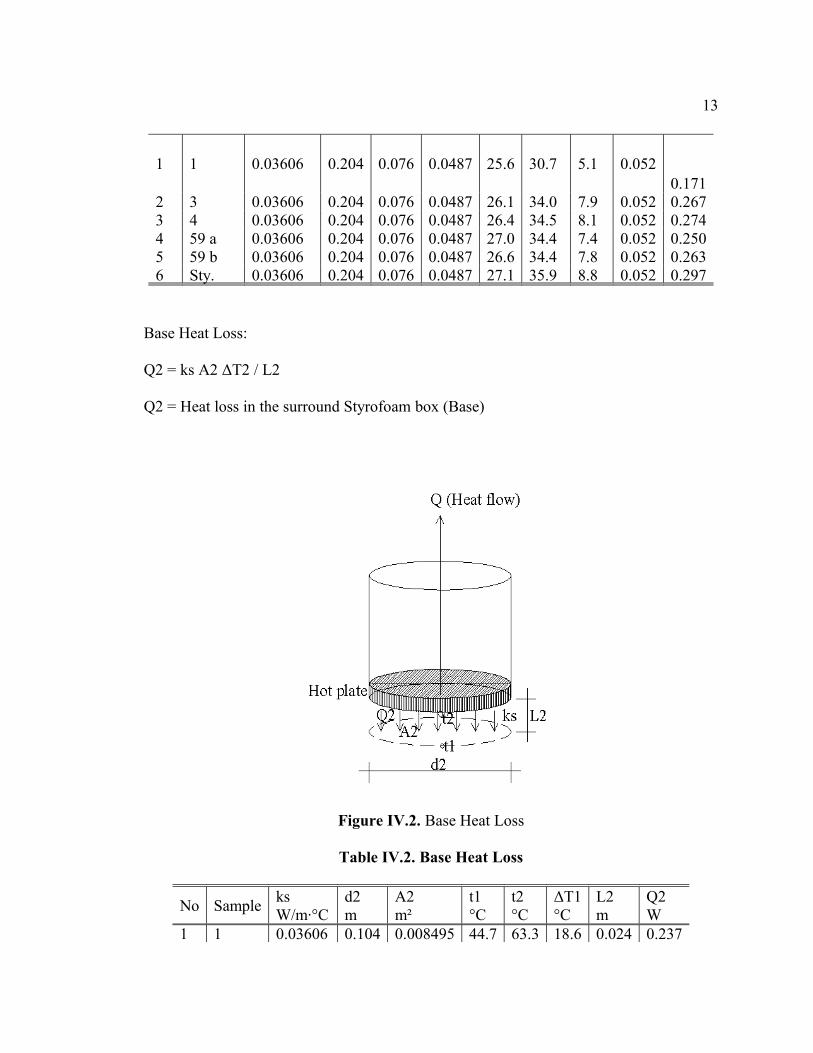
Base Heat Loss:

Q2 = ks A2 ΔT2 / L2

Q2 = Heat loss in the surround Styrofoam box (Base)

Figure IV.2. Base Heat Loss

Table IV.2. Base Heat Loss

No Sample ksW/m·°C

d2m

A2m²

t1°C

t2°C

ΔT1°C

L2m

Q2W

1 1 0.03606 0.104 0.008495 44.7 63.3 18.6 0.024 0.237

13

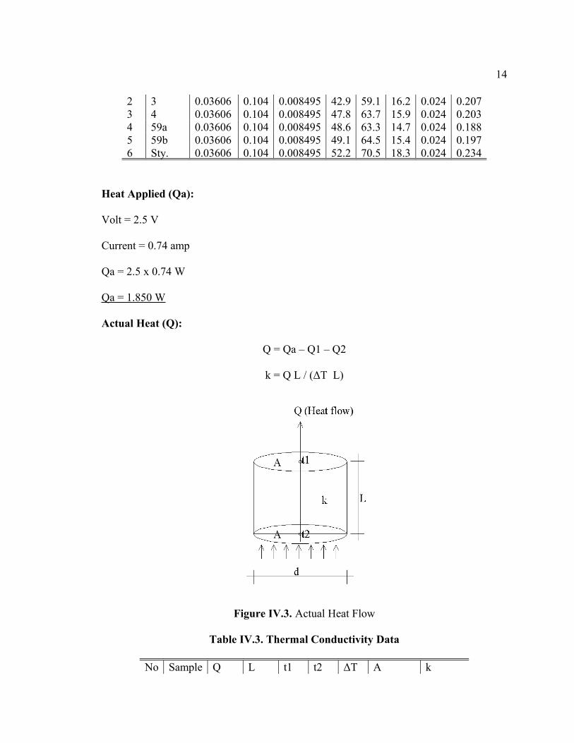
2 3 0.03606 0.104 0.008495 42.9 59.1 16.2 0.024 0.2073 4 0.03606 0.104 0.008495 47.8 63.7 15.9 0.024 0.2034 59a 0.03606 0.104 0.008495 48.6 63.3 14.7 0.024 0.1885 59b 0.03606 0.104 0.008495 49.1 64.5 15.4 0.024 0.1976 Sty. 0.03606 0.104 0.008495 52.2 70.5 18.3 0.024 0.234

Heat Applied (Qa):

Volt = 2.5 V

Current = 0.74 amp

Qa = 2.5 x 0.74 W

Qa = 1.850 W

Actual Heat (Q):

Q = Qa – Q1 – Q2

k = Q L / (ΔT L)

Figure IV.3. Actual Heat Flow

Table IV.3. Thermal Conductivity Data

No Sample Q L t1 t2 ΔT A k

14

W m °C °C °C m² W/m·°C1 1 1.442 0.076 25.3 57.8 32.5 0.008495 0.402 3 1.376 0.076 26.2 53.9 27.7 0.008495 0.443 4 1.373 0.076 25.8 58.0 32.2 0.008495 0.384 59a 1.412 0.076 26.7 59.6 32.9 0.008495 0.385 59b 1.390 0.076 25.5 59.8 34.3 0.008495 0.366 Sty. 1.319 0.076 26.2 66.3 40.1 0.008495 0.29

Thermal Conductivity Correction Factor (λ):

The Styrofoam sample is used as “bench mark” of known k = 0.03606W/m·°C.

Therefore, a correction factor (λ) is used to adjust the papercrete sample values of thermal

conductivity.

λ = 0.03606 / 0.29

λ = 0.12434

k corrected = λ k

R = L / k

TABLE IV.4. R values per inch

No Sample kW/m·°C λ

k correctedW/m·°C

Lm

RSIm²·°C/W

R-valueft²·°F·h/Btu

1 1 0.40 0.12434 0.04974 0.0254 0.51 2.92 3 0.44 0.12434 0.05471 0.0254 0.46 2.63 4 0.38 0.12434 0.04725 0.0254 0.54 3.14 59a 0.38 0.12434 0.04725 0.0254 0.54 3.15 59b 0.36 0.12434 0.04476 0.0254 0.57 3.2

15

0

10

20

30

40

50

60

70

0 50 100 150 200 250 300Time (min)

Temp (C) PapercreteSample 1

Top

Bottom

ΔT

FIG. IV.4. Thermal Conductivity Test Sample 1

16

0

10

20

30

40

50

60

70

0 50 100 150 200 250 300Time (min)

Temp (C) PapercreteSample 3

Top

Bottom

ΔT

FIG. IV.5. Thermal Conductivity Test Sample 3

17

0

10

20

30

40

50

60

70

0 50 100 150 200 250 300Time (min)

Temp (C) PapercreteSample 4

Top

Bottom

ΔT

FIG. IV.6. Thermal Conductivity Test Sample 4

0

10

20

30

40

50

60

70

0 50 100 150 200 250 300Time (min)

Temp (C) PapercreteSample 59a

Top

Bottom

ΔT

FIG. IV.7. Thermal Conductivity Test Sample 59a

18

0

10

20

30

40

50

60

70

0 50 100 150 200 250 300Time (min)

Temp (C) PapercreteSample 59b

Top

Bottom

ΔT

FIG. IV.8. Thermal Conductivity Test Sample 59b

19

0

10

20

30

40

50

60

70

0 50 100 150 200 250 300Time (min)

Temp (C) StyrofoamSample

Top

Bottom

ΔT

FIG. IV.9. Thermal Conductivity Test Styrofoam

20