Thermal Signature and Thermal Conductivities of PEM Fuel Cells - … · 2010-04-13 · enthalpy...
101
Odne Stokke Burheim Thermal Signature and Thermal Conductivities of PEM Fuel Cells Thesis for degree philosiphiae doctor Trondheim, August 2009 Norwegian University of Science and Technology Faculty of Natural Science and Technology Department of Chemistry
Transcript of Thermal Signature and Thermal Conductivities of PEM Fuel Cells - … · 2010-04-13 · enthalpy...

Odne Stokke Burheim
Thermal Signature and Thermal Conductivities of PEM Fuel Cells
Thesis for degree philosiphiae doctor
Trondheim, August 2009
Norwegian University of Science and Technology
Faculty of Natural Science and Technology
Department of Chemistry

NTNU
Norwegian University of Science and Technology
Thesis degree philosophiae doctor
Faculty of Natural Science and Technology
Department of Technology
© Odne Stokke Burheim
ISBN 978-82-471-1856-6 (printed version)
ISBN 978-82-471-1857-3 (electronic version)
ISSN 1503-8181
Doctoral theses at NTNU 2009:226
Printed by NTNU-trykk

Acknowledgement
First of all I would like to thank Professor Signe Kjelstrup, Dr. Preben J. S. Vie and Dr. Steffen Møller-Holst for believing in me and for giving me the opportunity to join the work on the “Thermal Effects in Fuel cell”-project, supported by the Norwegian Research Council grant number 164466/S30. I thank Preben Vie in particular for being so patient with me and for all the little tricks needed in the lab. Signe Kjelstrup has in addition to coaching and backing me up whenever needed also become a good friend and I thank her for sharing experiences from her own life.
Additionally, Jon Pharoah entered the group as a guest researcher in 2008. I thank him for spending so much time with me and teaching me that thinking takes time. The work would never have reached the present quality level without him.
I would further like to thank all my colleagues (students included) at NTNU and SINTEF who has surrounded me and supported me on a daily basis and for making it a pleasant time during these four years. A special thanks to Terje Bruvoll and Roger Aarvik for all help with administrative and practical tasks. All apparatuses custom made was manufactured by Ketil Joner in the workshop of the faculty and his advices in the process of designing these were much appreciated. I thank internship students Hannah Lampert and Karl-Heinz Heffels for their contribution to the experimental work and for all the fruitful discussions.
To my friends, whether we’ve been climbing together, shared flat or just hanging out, thanks for all support and the great times you have given me. A special thank to Ole-Erich Haas for the years together in university and in particular the last six years. Spending long days in the lab for our master degrees and studying all day long for exams have been of great significance for several reasons.
At some point, Ragnhild turn up in the office next to mine. She completes my life and is such a pleasure to be with. I thank her for being so patient when my mind obviously is somewhere else or I just want to stay an extra minute. I am really looking forward to spend my life together with her.
Finally, I would like to thanks my mom, my dad and my sister for always standing up for me and for supporting all activities now and in my childhood. Being encouraged to read, learn and use my curiosity for exploration has made me who I am and has been essential for my choice in career.


Summary of work
The work presented here gives estimates on thermal gradients within the PEM fuel cell, an experimental route to measure the through-plane thermal conductivity of the materials used in the PEM fuel cell and also suggestions of which material characteristics which should be aimed for with respect to thermal management of fuel cells. The work reports for the first time how the thermal conductivity of Nafion® changes with water content. An effect residual water has on the thermal conductivity of the PTL is also reported for the first time. In addition to this a calorimeter for the PEMFC was constructed to measure the thermal signature. This is also reported for the first time in the literature.
To elucidate the heat gradients possible within a PEM fuel cell and to better understand the calorimetric measurements, a 2D thermal model was created and applied at different conditions. The model was made by the use of the finite element method software COMSOL 3.3. This model was used to evaluate temperature elevations in the single cell mainly imposed by water transport, component thermal conductivity modifications and gas flow channel design. The 2D model was compared to a 1D model to demonstrate the importance of taking the gas flow channel design into account. For simplicity, many illustration models consider only 1D. Parallel gas flow channels tend to impose an increased current density under the gas channel while serpentine flow channel pattern does the opposite, according to several studies. Thus a simple 2D model can, as very good approximation, be used to study effects rising from 3D cell designs. It was demonstrated that parallel flow fields give a higher maximum temperature than serpentine gas flow channels. Changes in the porous transport layer, such as compression, residual water and increased through-plane thermal conductivity were also discussed. In general, the maximum temperatures predicted for the PEM fuel cell were between 4.5 and 15 K above the control temperature in the polarisation plate, depending on the conditions in the model.
One of the motivations for the thermal model of the fuel cell was to demonstrate the importance of measuring the through-plane thermal conductivity of fuel cell components. An apparatus for these measurements was constructed and is reported in the presented work. Using K-type thermocouples and digital micrometers together, the apparatus had the possibility to measure the variables in Fourier’s law; the heat flux through the sample, the temperature difference over the sample and its thickness. The thermal conductivity of Nafion® was measured at room temperature as a function of water content; found to be 0.177 ± 0.008 and 0.254 ± 0.016 W K-1 m-1 for dry and maximally wetted membranes respectively. The membrane thickness and thermal conductivity showed no response to increased compaction pressure. The thermal conductivity of the chosen PTL (supplied from Sigracet) was measured both dry and saturated with liquid water at different compaction pressures. The chosen PTL’s through-plane thermal conductivities was measured to be 0.27, 0.36 and 0.40 W K-1 m-1 at 4.6, 9.3 and 13.9 bar compaction pressure respectively. By saturating the PTL with liquid water, the thermal conductivity increased up to 70 %. By measuring the

thickness of the uncompressed PTL, it was observed that the thickness changed by 70 μm depending on the location on the PTL. This corresponds to more than ten percent relatively speaking.
Having used the model to see the effects rising from manipulating some of the experimentally measured data, several commercial PTLs were gathered and measured in order to create a small database of through-plane thermal conductivities and thermal contact resistivities. Depending on the brand, compaction pressure, Teflon content and liquid water content the material conductivity and thermal contact resistivities were found to be 0.15-1.6 W K-1 m-1 and 0.7 – 11.1 10-4 K m2 W-1, respectively. Though some efforts exists, both experimental and theoretical, there is yet no data collection concerning the PTL thermal conductivity as broad, detailed and brand specific as the present in the literature. In addition to this the study opens up for a mechanistic study on how water and Teflon seem to affect the over all heat conduction.
As a part of the thermal studies of PEMFCs, a calorimeter was constructed. The construction and the use of the calorimeter may be regarded as a second motivation for the thermal fuel cell modelling, hoping it would lead to a better understanding of the possibilities and limitations of the calorimeter. The calorimeter measured both the heat and the available work from the fuel cell reaction at constant pressure. As is well known, the sum of these two is equal to the enthalpy of the cell reaction. The control temperature was kept at 50 oC, in order to make sure that the product water would leave the fuel cell in its liquid state. It is important to state this because the reaction enthalpy depends on the state of the product. The most important result from this experiment is that the enthalpy of the fuel cell reaction was measured to be linearly dependent on the fuel cell potential for cell potentials less than 0.55 V, even though the product water was in its liquid state. The only reasonable explanation is that the recorded enthalpy is a mixture of two reactions: formation of water and formation of hydrogen peroxide. At cell potential 0.3 V the calorimetric measurement revealed that the recorded reaction enthalpy corresponds to production of more than 15 mol% hydrogen peroxide. As the formation of hydrogen peroxide is not recorded in-situ until now, this demonstrates one of the advantages of calorimetric measurements. It was further demonstrated that the deviation in the fuel cell reaction enthalpy can be linked both to the inflection point in the polarisation curve and thus also the rapid fall in the power curve. For the cell potentials above 0.55 V the approach demonstrated that the Tafel overpotential can be recorded from the thermal signature.

Nomenclature
Roman Letters
a V Tafel constant
b V / decade Tafel slope
j A cm-2 Current density
jo A cm-2 Exchange current density
ki W K-1 m-1 Thermal conductivity
l m Length
n
Number of electrons in the reaction
p bar Pressure of gas
q J Heat change between two states
qi W m-2 Heat flux
ri K W-1 m-1 Thermal resistance per unit length
xi
Mol fraction of component i
Ai m2 Area
Eo V Standard state potential
Ecell V Cell potential
Erev V Reversible potential
ETN V Thermoneutral potential
Nomenclature vi
F C mol-1 Faraday constant
G J mol-1 Gibbs energy
H J mol-1 Enthalpy
I A Current
P W cm-2 Electric power
Q W cm-2 Heat production
R J mol-1 K-1 Gas constant
Ri K W-1 / Ω cm2 Thermal resistance / Electric resistivity
R”i m2 K W-1 Thermal resistivity
S J mol-1 K-1 Entropy
T K or oC Temperature
U J mol-1 Internal energy
V m3 Volume
W J mol-1 Work
Z m or μm Thickness
Greek Letters
α Transfer coefficient
α H2O per H+ Net water drag in a PEMFC
ζ H2O per H+ Water product multiplier
vii
η V Over-potential
λ H2O per –SO3+ Water content in Nafion® membrane
σ A cm-2 Amplitude of j-distribution
Δ Difference between two states
Ω ohm cm2 Electric resistivity
Subscripts and Abbreviations
AFC Alkaline Fuel Cell
BPP Bipolar Plate
FF / FC Flow Field / Gas Flow Channel
HP High Pressure
MCFC Molten Carbonate Fuel Cell
MEA Membrane Electrode Assembly
MPL Micro Porous Layer
PAFC Phosphoric Acid Fuel Cell
PEEK Poly Ether Ether Ketone
PEMFC Polymer Electrolyte Membrane Fuel Cell
PP Polarisation Plate
PTFE Teflon (Poly Tetra Fluor Ethylen)
PTL Porous Transport Layer

Nomenclature
viii
SOFC Solid Oxide Fuel Cell
TtW Tank to Wheel
WtT Weel to Tank
WtW Well to Wheel

Contents Acknowledgement.........................................................................................................................................i Summary of work........................................................................................................................................iii Nomenclature ...............................................................................................................................................v Contents.......................................................................................................................................................ix 1 Introduction ...........................................................................................................................................1
1.1 Background ....................................................................................................................................1 1.1.1 Fuel cell technologies ...........................................................................................................2 1.1.2 Fuel cells answer to needs in the future................................................................................3 1.1.3 History of Fuel Cells.............................................................................................................5
1.2 Aim and outline of the Thesis ........................................................................................................6 2 On the Temperature Distribution in Polymer Electrolyte Fuel Cells ....................................................9
2.1 Introduction..................................................................................................................................10 2.2 A 2D Thermal Model ...................................................................................................................12
2.2.1 The problem geometry........................................................................................................12 2.2.2 Thermodynamic background ..............................................................................................13 2.2.3 Model Formulation .............................................................................................................14
2.3 Model Results ..............................................................................................................................17 2.3.1 The nature of the system.....................................................................................................17 2.3.2 The effect of water..............................................................................................................20 2.3.3 Material thermal conductivities ..........................................................................................22 2.3.4 Flow field design ................................................................................................................23 2.3.5 Lost work in the PEMFC fuel cell. .....................................................................................26 2.3.6 Stack considerations ...........................................................................................................27
2.4 Conclusions..................................................................................................................................28 3 Ex-situ measurements of through-plane thermal conductivities in a polymer electrolyte fuel cell .....29
3.1 Introduction..................................................................................................................................30 3.2 Experimental ................................................................................................................................32
3.2.1 Apparatus............................................................................................................................32 3.2.2 Procedure............................................................................................................................35 3.2.3 Statistical analysis...............................................................................................................38
3.3 Results..........................................................................................................................................38 3.3.1 Thickness measurements ....................................................................................................38 3.3.2 The thermal conductivity of Nafion® as a function of water content..................................40 3.3.3 Thermal conductivity of the Porous Transport Layer.........................................................42 3.3.4 Thermal resistance of the single PEMFC ...........................................................................44
3.4 Discussion ....................................................................................................................................45 3.4.1 Thermal conductivity of Nafion® .......................................................................................45 3.4.2 Thermal conductivity of the Porous Transport Layer.........................................................45 3.4.3 Thermal conductivity of the single PEMFC .......................................................................46
3.5 Conclusion ...................................................................................................................................47 4 Through-Plane Thermal Conductivity of PEMFC Porous Transport Layers (GDLs).........................49
4.1 Introduction..................................................................................................................................50 4.2 Experimental and modelling ........................................................................................................51 4.3 Results..........................................................................................................................................51
4.3.1 Carbon Papers.....................................................................................................................52 4.3.2 Carbon felts ........................................................................................................................56
4.4 Discussion ....................................................................................................................................58 4.5 Conclusions..................................................................................................................................60
5 A calorimetric analysis of a polymer electrolyte fuel cell and the production of H2O2 at the cathode61 5.1 Introduction..................................................................................................................................62 5.2 Theory ..........................................................................................................................................65 5.3 Experimental ................................................................................................................................69
5.3.1 Apparatus............................................................................................................................69 5.3.2 Measurement ......................................................................................................................71

Content
x
5.3.3 Data reduction procedure....................................................................................................72 5.4 Results and Discussion.................................................................................................................73
5.4.1 The reaction enthalpy .........................................................................................................73 5.4.2 The cell power and the polarisation curve ..........................................................................77 5.4.3 The overpotential from the polarisation curve and the thermal signature...........................78
5.5 Conclusions..................................................................................................................................80 6 Conclusions and further work .............................................................................................................81
6.1 Conclusions..................................................................................................................................81 6.2 Further work.................................................................................................................................82
Bibliography...............................................................................................................................................85


1 Introduction
1.1 Background
Fuel cells offer a solution where renewable energy, stored as produced hydrogen, can replace today’s use of oil in greater parts of the transportation sector. This change will become a necessity for a number of reasons.
According to the Medium-Term Oil Market Reports, MTOMR, of the International Energy Agency, IEA, the average production rate of all existing oil fields in the world is decreasing. [1] The potential production rate of these was reported to decrease by 4 % and 7 % in the MTOMR of 2007 and 2008 respectively. To meet the increased demand for oil products in the market the number of oil fields is being increased. However, the production capacity of new oil fields do not match up to those previously developed and, additionally, they are often more technically sophisticated to produce so that delays of the start-ups has increasingly become a significant problem. One result of this situation is that the estimated point of world production peak is annually being brought closer to our time. Whether the oil production peak is in five years or in fifteen years is of less significance, however, when it is clear that we, as a worldwide society, can not for much longer lean upon oil as the main energy source for transportation.
From some of the scenarios given by the International Panel on Climate Change, IPCC, there is little doubt that care should be taken when using oil and other fossil fuels as energy sources. [2] Not mainly due to the non sustainable future of the supply source, but simply because we are closing onto the point of no return for the changes in global climate.
Of course, fuel cell and hydrogen production is not the only solution to the problems mentioned. Alternatively, synthesized diesel from coal and bio-fuels can replace today’s use of oil. However, there are ethical arguments against bio-fuels, such that agricultural lands should rather be used to feed our world’s growing population. Coal based diesel production (Fischer-Tropsch synthesis) is a source of green house gas emissions and this alternative depends on carbon capture to avoid the climate change arguments.

Chapter 1. Introduction 2
1.1.1 Fuel cell technologies
Fuel cells are in many ways similar to batteries. The exception is that the chemicals required for the reaction are continuously being replaced or refilled.
The PEM fuel cell.
A cross sectional sketch of polymer electrolyte membrane fuel cell, PEMFC, is depicted in Figure 1. This is the type of fuel cell which this thesis focuses on. It uses humidified hydrogen as a fuel and together with oxygen (or air) the chemical energy is converted to electric energy, though humidification of hydrogen is not always necessary. The PEM fuel cell is usually operated between 50 oC and 80oC, and is therefore regarded as a low temperature fuel cell.
Figure 1 A classical PEM Fuel Cell sketch, depicting how mass and electricity are exchanged.
The PEM fuel cell sketched in Figure 1 is fed with humidified hydrogen on the anode side of the membrane. The hydrogen gas, H2, streams through channels in an electronic conductive support before it is further distributed over the membrane area. This support is usually called a polarisation plate and the channels are often named gas flow channel or gas flow field. To distribute the gas one applies a porous layer, which is also electronically conductive – sometimes (and for this work) termed the Porous Transport Layer, PTL. Between the PTL and the membrane the hydrogen gas comes in contact with the catalytic layer, and is oxidised into electrons, e-, and protons, H+. This layer is one of the electrodes in the PEMFC. The catalytic layer consists of carbon, membrane polymer and catalyst. This layer is typically 20 microns thick. Because the membrane doesn’t conduct electrons, only the protons enter the membrane and further move over to the cathode side. The proton conductivity in the membrane is enhanced by presence of water and the protons tend to drag water along to the cathode, hence the
H3O
+ Membrane
H2O 2 H2 → 4 H+ + 4 e- PTL
H2O O2 + 4 H+ + 4 e- → 2 H2O PTL
External load, e.g. ; cars buses mobile devices Etc…
Anode
O2 & H2O
O2 & H2O
O2 & H2O
O2 & H2O
O2 &H2O
O2 & H2O
H2 & H2O
H2 & H2O
H2 & H2O
H2 & H2O
H2 & H2O
H2 & H2O
Cathode

1.1 Background 3
humidification of the hydrogen gas. The electrons are conducted through the PTL and the support to an external load. The electrons enter the fuel cell in a similar manner on the cathode side of the fuel cell. On this side, the electrons meet protons and oxygen in the catalytic layer and spontaneously and instantaneously form water. This layer is thus the other electrode in the fuel cell. The oxygen gas enters the fuel cell in the same manner as the hydrogen, while water leaves in the opposite direction. Thus, air flowing through the flow channels on the cathode side enters dry and rich on oxygen and leaves humidified and lean on oxygen.
Due to the demands of the fuel cell process, the interfacial region between the electrodes and the PTL can be more diverse than so far explained. The fuel cell reactions in each of the catalytic layers require simultaneously a reactant gas along with an electronic and an ionic conductor. For the membrane to optimally conduct protons, water must be accessible. In order to supply water to the membrane and at the same time give the reactant gases a path to the catalyst layer an impregnate layer is attached between the catalyst layer and the PTL. This layer is typically 50 μm thick and consists of a mixture of Teflon and carbon black (nano sized carbon particles) forming tiny pores. The layer is usually referred to as the Micro Porous Layer – MPL. Due to capillary forces in many of these tiny pores, water droplets are forced to stay on each side of this layer. The MPL gives the PEMFC significantly improved performance and is therefore used in most fuel cells.
Other fuel cells
In addition to the PEMFC, there is several other types of fuel cells worth to mention. The differences are given by the fuels fed to the cell, the membrane conductive mechanisms and region of operation temperature. The Solid Oxide Fuel Cell, SOFC, has a membrane made of a solid oxide, usually Y0.1Zr0.9O2, capable of conducting oxygen ions. It is often fed with natural gas and is operated with temperatures between 900 oC and 1000 oC. The Molten Carbonate Fuel Cell, MCFC, has a liquid electrolyte consisting of carbonate salt, e.g. NaCO3, and has thus the ability to conduct oxygen ions along with CO2, which is fed together with the oxygen and reused by extraction from the anode exhaust. It is fed with natural gas or hydrogen gas and operated around 600 oC. Phosphoric Acid Fuel Cells, PAFC, conducts protons by using liquid phosphoric acid as the electrolyte and operates at 150 – 200 oC. Alkaline Fuel Cells, AFC, uses an alkaline liquid electrolyte, such as potassium hydroxide, which transports oxygen as hydroxide ions (cathode reaction: ½ O2 + H2O + 2e- ↔ 2 OH-). This fuel cell is, like the PEMFC, a low temperature fuel cell that must be fed with hydrogen to work properly. The advantage of the low temperature fuel cells is that they are easy to start up and shut down, while their drawback is that they are sensitive to chemical pollutions, such as carbon oxides.
1.1.2 Fuel cells answer to needs in the future
Our entire society needs to convert to alternatives to oil for several reasons. The hydrogen society seems to be the most feasible alternative that includes the transport sector. The essence in the concept of a hydrogen society is the hydrogen economy

Chapter 1. Introduction 4
where hydrogen is used as an energy carrier, where electricity converted into hydrogen and further stored or sold and used. An example of a hydrogen society is illustrated in Figure 2.
Hydrogen is found chemically bound to other elements all over the planet. Water and all organic material in our surrounding contain hydrogen. It is not only due to the substance being so omnipresent and abundant that hydrogen is repeatedly mentioned as the successor of today’s fossil products. The simplicity of extracting hydrogen from water can even be demonstrated by child with a battery, two metal wires and glass of salinated water. Hydrogen has the largest energy of combustion per unit of mass, and is therefore ideal for the transport sector. [3] As illustrated in Figure 2, electricity, bio-mass or natural gas can be used to extract hydrogen gas which is further stored until use for electricity production via a fuel cell route. The hydrogen can also be used for an Internal Combustion Engine, ICE. Both technologies used in a hydrogen society will have to compete with batteries, though they apply to somewhat different market areas.
When energy efficiency of various technologies in the transport sector are compared, three efficiency terms are commonly used; Well to Tank – WtT, Tank to Wheel – TtW and Well to Wheel – WtW. The third one is the product of the first and second. The word well is used as a metaphor for the energy source, e.g. wind turbine, nuclear power plant, gas resource, hydro power station, etc. Today, oil wells are the most common energy tap for the transport sector. Due to refining and distillery costs, WtW is commonly used in evaluating production costs. A comparison between possible hydrogen based technologies is given by Svensson et al and shown in Table 1 [4]. The WtW analysis shows that fuel cells have twice the energy of efficiency of an ICE hydrogen car and more than a third of an electric car. Solely based on energy efficiency, it is clear that fuel cells are more feasible than the hydrogen ICE. In addition to this the reaction temperature in the hydrogen ICE causes release of nitrogen oxides, NOX. When considering the competition between fuel cells and Li-ion batteries one must consider the needs for rapid energy recovery in the transport sector. While a tank of hydrogen can be filled within very few minutes, batteries require charging for several hours. This is the main advantage of the PEM fuel cell; it is the most efficient alternative when considering filling time, global environment and the fuel options of the future.

1.1 Background 5
Table 1 A comparison on energy efficiency of passenger vehicles in a possible hydrogen society. [4]
WtT* TtW WtW
ICE on H2, 700 bars 69 % 20 % 14 %
PEMFC on H2, 700 bars 69 % 40 % (50 %)** 28 % (35 %)**
Li-ion Batteries 83 % 89 % 74 %
* includes loss in distributing electricity on net grid, ** hybrid to battery
Electricity production Renewable Nuclear Fossil
Hydrogen Production Bio-mass
Natural gas Stored hydrogen
FC
FC
FC
FC
Figure 2 A schematically explanation of energy floating as electricity and hydrogen in the hydrogen economy/society.
1.1.3 History of Fuel Cells
In order to give readers a perspective on the history of fuel cell development, a brief summary of the time line is given below. [5]
1839: Christian Friedrich Schönbein and Sir William Robert Grove reports separately on the fuel cell effect in the papers “On the Voltaic Polarization of certain

Chapter 1. Introduction
6
Solid and Fluid Substances” and “On voltaic Series and the Combination of Gases by Platinum” respectively.
1842-1845: Sir Grove constructs a fuel cell generator which he refers to as “Gaseous Voltaic Battery”. The generator was described in several papers. The work continued for several more years after this, though it failed in the competition with steam engines and ICE.
1930s: Francis T. Bacon starts his work developing the alkaline fuel cell (1932). In the later part of the decade the interest in SOFC rouse, based on work done on solid oxide conductors performed by Nernst late in the previous century.
1950s and 1960s: The fuel cell gained a renaissance as space travel programs required energy solutions offered by fuel cells. Low temperature fuel cells supplied both electricity and water for drinking and atmospheric humidification. AFC where used for the Apollo program and the Space Shuttles, while the PEMFC where used only for the Gemini Earth-orbiting programs in the mid 60s. At this point, the PEM technology still struggled with poor membrane development and was therefore not chosen for further space programs.
1970s: Oil shortage in this period woke up an interest in fuel cells for commercial purposes and several companies and organizations started to intensify their effort into this research. Development of PAFCs and Nafion® formed the foundation for the boom fuel cells have had the last 10 – 15 years.
1.2 Aim and outline of the Thesis
This doctoral work is a part of the project “Thermal Effects in Polymer Electrolyte Fuel Cells”, granted by the Norwegian Research Council. The project is collaboration between NTNU, SINTEF and IFE and aims to study how PEM fuel cells deviate from the assumption of being isothermal. As a part of that project, the work presented in this thesis focuses on thermal conductivity measurements of fuel cell components, calorimetric measurements of a PEM fuel cell and also thermal modelling of temperature profiles in a PEMFC.
The presented work originates from work previously done by Vie, Møller-Holst and Kjelstrup. [6] [7] [8] Vie, by inserting a 280 μm thick thermo-couple between the membrane and the PTL, observed that the temperature of the catalyst layer and the membrane is several degrees above the control temperature at the backing plate. He was also able to give rough estimates on the thermal conductivities of some of the fuel cell components. Møller-Holst, in order to increase his understanding of the heat production in the fuel cell, constructed a simple calorimeter for the PEM fuel cell.
The work presented in this thesis was planned to support and further improve the experimental accuracy of previous work performed by these two gentlemen. Knowledge and understanding of the thermal conductivity of fuel cell materials is of great importance when engineering materials and operating fuel cells. We aimed to obtain new experimental data not previously reported. Further, our intention was to

1.2 Aim and outline of the Thesis 7
design, build and use a calorimeter as an in-situ technique for studies of reaction mechanisms.
Chapter 2: This chapter studies the heat production in a PEM fuel cell by the use of a 2D thermal model. Several aspects and likely scenarios are considered and the main results are given as maximum temperatures in a PEMFC. This chapter explains the need for the thermal studies in order to improve the understanding and engineering of PEM fuel cells. This chapter originates from and is inspired by the work presented in Chapter 3 and 5.
Chapter 3: One of the goals with this work was to create a steady routine for measuring through-plane thermal conductivity of PEMFC components. A description of an experimental approach to measure thermal conductivity for fuel cell components with thicknesses ranging from 50 μm to 2 mm is given as the result of this work. Due to the accuracy of the measured thickness, we measured both the thermal conductivity and the thermal contact resistance to the apparatus at different compaction pressures for both PTL materials and Nafion®. We measured the thermal conductivity of Nafion® as a function of water content and the thermal conductivity of GDL with and without residual water. None of these results has previously been reported in the literature.
Chapter 4: As a result from the work in chapter two and three, a desire for a broader and more detailed PTL thermal conductivity data base appeared. Thus we put together more than ten different materials to see how fibre structure, Teflon content and residual liquid water affected the through-plane thermal conductivity. Investigating this material collection, a new broader, more detailed and more brand specific data base than what is presently available was created. The study allows for fuel cell researchers to create better models and a improve their understanding of heat transfer mechanisms in the porous transport layers.
Chapter 5: The aim of the calorimeter was to study reaction mechanisms from the fuel cell thermal signature. The heat and work from a PEMFC was measured and reported for various at different current densities and cell potentials. We demonstrate that the Tafel behaviour can be obtained from the thermal signature, but more important is that it is demonstrated that the inflection point in the polarisation curve is directly linked to a drop in the fuel cell reaction enthalpy and further the formation of hydrogen peroxide. This result was not previously reported in the literature, though the hydrogen peroxide formation is reported by others.
Each of the chapters 2, 3 and 4 has been written as independent parts and are published in or submitted to scientific journals.


Chapter 2
2 On the Temperature Distribution in Polymer Electrolyte Fuel Cells
Odne Burheim and Jon G. Pharoah
Department of Chemistry
Norwegian University of Science and Technology
N-7491 Trondheim, Norway
This manuscript has been submitted to
J. Power Sources (2009.08.25)

Chapter 2. On the Temperature Distribution in Polymer Electrolyte… 10
ABSTRACT
This paper presents 2D thermal model of a fuel cell to elucidate some of the issues and important parameters with respect to temperature distributions in PEM fuel cells. A short review on various properties affecting the temperature profile and the heat production in the polymer electrolyte fuel cell material is included. At an average current density of 1 A cm-2, it is found that the maximum temperature of the MEA is elevated by between 4.5 K and 15 K compared to the polarisation plate temperature. The smallest deviation corresponds to one dimensional transport, while the largest corresponds to the two dimensional transport considering anisotropic thermal conductivity. The two dimensional thermal model further predicts increased lost work. While most of the heat generation is allocated in the cathode, it is shown that the heat effect may be balanced by the water phase change in the anode. The most significant factor in determining the temperature distribution is the channel width, followed by the thermal conductivity of the porous transport layer and state of water in the cell.
2.1 Introduction
The vast majority of fuel cell work, both experimental and theoretical, assumes isothermal conditions when in reality isothermal conditions are extremely difficult to maintain, especially at moderate and high current densities. Single cells are often externally heated during experiments while stacks require significant cooling and temperature gradients will exist both within a cell and within the stack. Understanding the temperature distribution is important as the lost work from reversible heat is temperature dependant, but also because the membrane may be exposed to its glass transition temperature. In addition, elevated temperatures contribute to degradation rates which can be exacerbated by high temperatures and large gradients. Further, the effect of water phase change can, depending on the rate, have a significant impact on the resulting temperature distributions.
The operating temperature of a fuel cell is usually taken to be the temperature measured at some distance from the electrodes, often in the end plate, and this value can be significantly different from temperature at the electrodes. In fact, some measurements have shown that the temperature in the gas channels can be as much as 8 °C cooler than that adjacent to the electrode itself [6]. While the effects are smaller, this trend is also demonstrated in non-optimized cells with unique temperature sensors impeded in the electrolyte [9]. Knowing the actual temperatures at the electrodes is important for several reasons: a) the reaction kinetics are dependent upon the temperature of the electrode, b) the transport properties are functions of the local temperature c) the rate of phase change is strongly dependent on the local temperature and d) Nafion electrolytes must reasonably be maintained below 120 °C at 1 atm to avoid irreversible damage by humidified air [10].

2.1 Introduction 11
According to Bauer et al. [10], [11] Nafion will significantly and permanently decrease its ionic conductivity at elevated temperature. The elastic strength of Nafion, the E-modulus, was measured both as a function of temperature and as a function of access to water. This property is lowered by increased temperature and increased water accessibility. When the E-modulus is sufficiently weakened and water is adequately accessible, the membrane material will swell to self destruction. Nafion is resistant to failure by temperature elevation if the access to water is limited. It was revealed that Nafion exposed to 100 % RH at 1 atm will undergo irreversible damages at 120 oC. Between 90 and 95 oC Bauer et al. found that the E-modulus of Nafion in contact with liquid water started to decrease dramatically with increased temperature. This result suggests that Nafion in contact with liquid water at approximately 95 oC may undergo detrimental changes. Further, it was shown that by lowering the relative humidity the maximum temperature recommendation for Nafion would increase, i.e. at 1 atm approximately 91 % RH / 130 oC, 85 % RH / 140 oC and 75 % RH / 150 oC. Taking into account Nafions response to temperature elevation, water accessibility and that water is liquid up to almost 120 oC (for gases at 2 atm), a PEMFC may, in this region (90-120 oC), be irreversibly damaged. The temperature range chosen for the measurements [10] may have been based on an understanding that the fuel cell was isothermal, as was the general perception around 2001.
The factors which significantly affect the temperature distribution include: 1) component conductivities, 2) contact resistance, 3) heat losses from the system, 4) the electrode reactions, 5) the local rate of water phase change and 6) the geometry of the cell. Point one and two refers to the selected materials for the cell, the compaction forces and the local environment, i.e. residual water. Recently, Burheim et. al [12] demonstrated how the increasing compaction pressure and residual water in the PTL increases the through-plane thermal conductivity of PTLs. However, these results consider only the through-plane thermal conductivity. According to Ramousse et al. [13], based on the model by Danes and Bardon, the in-plane thermal conductivity of a PTL should be between ten and twenty times the through-plane thermal conductivity, depending on the fibre structure. Ironically, Danes and Bardon developed the model for porous carbon fibre felts intended for insulation [14]. However, measurements of in-plane thermal conductivities are not yet reported. Because measurements of through-plane thermal conductivity support the modelling work by Ramousse and Bardon, it is very likely that that the PTL is highly anisotropic, though the in-plane thermal conductivity may not depend on compaction pressure and residual water to the same degree as the through-plane thermal conductivity.
The lost work in the fuel cell, i.e. ohmic heating and the overpotential, as well as the local rate of water phase change will depend on local temperatures and current density deviations in the fuel cell. Pharoah et al. [15], [16] report that, if running a fuel cell at moderate to high current densities, a serpentine gas flow channel will give decreased current underneath the channel while parallel flow fields will have the opposite effect. The prediction is based on modelling a half cell, using an air cathode. Reum et al. [17] report measurements of similar effects for a fuel cell using parallel gas flow channels. Running their fuel cell at moderate current densities of 0.4 A cm2 with fully humidified oxygen/hydrogen the maximum current densities underneath the gas

Chapter 2. On the Temperature Distribution in Polymer Electrolyte…
12
channel is twice the minimum current density below the lands. Replacing oxygen with air increases this effect so that the maximum current density is more than ten times the smallest.
Considering the effects the gas flow field design imposes to the current density distribution and that the MEA is literally insulated by its surrounding PTL, we present a 2D thermal model of a fuel cell to elucidate some of the issues and important parameters in fuel cell design. The goal of this paper is to present simple and efficient model to estimate the maximum temperature generated within a fuel cell, and those parameters which are most important in determining this maximum.
2.2 A 2D Thermal Model
A steady 2D thermal model is developed using the commercial finite element code COMSOL Multiphysics 3.3. A 1D thermal model was also developed, primarily for comparison to other 1D thermal models. This was done simply by removing the gas channels. We give the problem geometry first, the thermodynamics second and the model formulation at the end of this section.
2.2.1 The problem geometry
The domain of interest is depicted in Figure 3 and includes bi-polar plates, porous transport layers (sometimes also referred to as a gas diffusion layers) coated with micro porous layers, catalyst layers and a Nafion electrolyte. All dimensions are given in Figure 3. The gas flow channel geometry was chosen as a repetitive pattern, 1 mm x 1mm, except where otherwise noted. Thermal contact resistance is accounted for between the bi-polar plate, and the porous transport layer, but is currently neglected for all other interfaces.

2.2 A 2D Thermal Model 13
L
Figure 3 Problem geometry.
2.2.2 Thermodynamic background
In order to optimise a fuel cell, it is important to understand where potential work is lost. Equation 2.1 follows directly from the first law of thermodynamics written per unit time. The electric work per unit time extracted from the system at constant pressure is the power delivered by the fuel cell, PFC. Assuming that the reactants enter the system at the same temperature and pressure as the products leave the system, the change in internal energy is given by the change in free energy for the fuel cell reaction, G = H - TS. A real system will also lose heat to the environment, due to i) the energy needed to drive the electrochemical reaction (often referred to as activation losses), j, and ii) due to ohmic heating, Rj2. This can be expressed as the second half of Eq. 2.1, where the thermo-neutral voltage, Etn = H/nF expresses the total energy, and all other terms represent losses from the point of view of power extracted from the fuel cell. The term related to the entropy change for the reaction, TS, gives rise to a heat release which is reversible, Qrev while the other two terms are irreversible. For the
W
1.0 mm
Air
H2
Al B.P.P
Al B.P.P
PTL
PTL
M P L
M E M B R A N E
CATHODE
ANODE
M P L
250 μm 50 μm 20 μm 50 μm 20 μm 50 μm 250 μm
y x
25 μm into membrane

Chapter 2. On the Temperature Distribution in Polymer Electrolyte… 14
PEM fuel cell reaction the entropy is negative and the reversible heat represents lost work proportional to the temperature. We shall see how this reversible heat production is dependent on the local reaction temperature imposed by cell design and further the available electrochemical potential. We will also evaluate the lost work due to the activation overpotential by considering that it changes with current distributions imposed by gas flow channel design.
2 ' 'FC TN rev jP j j j Rj E j Q Q
nF nF 'H T SQ
(2.1)
2.2.3 Model Formulation
Since the goal of this work is to predict the temperature distribution within a fuel cell, we solve the heat diffusion equation over the domain shown above, and apply source terms to account for the heat generated by each of the mechanisms discussed above. One additional consideration however relates to the phase changes of water within the system. In considering the entropy and enthalpy changes for the fuel cell, a choice has to be made for the state of the product water. If water vapour leaves the system, then the enthalpy change is lower while if it leaves as liquid, it is higher by the heat of vaporisation of water. It is still possible however for water to undergo phase changes within the system which can significantly change the temperature distribution. These changes do not affect overall conservation of energy though, as long as water enters and leaves the system in the same phase and the appropriate enthalpy and entropy changes are used. In the present model, water profiles are not explicitly solved for but the temperature effects due to phase change of water are accounted for by assuming a net drag of water, , condensing (absorbing into the membrane) at the anode and a maximum of this water plus the electrochemically produced water, progressing to the vapour state by evaporation (desorption) at the cathode. Various assumptions about the state of water can be investigated by independently varying and . The water content in the membrane is considered to be homogeneously distributed.
The model considers only two dimensions, but different current distributions across the channel (in the y-direction) are imposed by the flow channel design and thus we can compare 3D-like flow channel designs. As discussed above, a serpentine flow field results in a maximum current underneath the land, while a parallel flow field results in a maximum current under the channel [15], [16], [17]. Here, we have chosen to impose characteristic distributions using half a period of a cosine function
1 cosj y j yW
(2.2)
where Wis the channel dimension and σ is the desired amplitude. Figure 4 depicts the cross-channel current density distributions used in this model. The amplitude

2.2 A 2D Thermal Model 15
of the distribution is relatively small (except for in one case) such that the results should predict the minimum effect of flow field on temperature distribution. The amplitude, , in Eq. 2.2 was chosen such that the temperature along the midline of the membrane was as constant as possible. Again, one exception was made; switching from oxygen to air and broadened flow channels and ribs appear to dramatically increase the amplitude in the current distribution [17]. The three current distributions are sketched in Figure 4, note that the x-axis in the figure is as the fractional length of the channel width (W = 1 and 2 mm).
0.0
0.5
1.0
1.5
0 0.2 0.4 0.6 0.8 1
y / Wchannel
j / A
cm
- 2
Serpentine, σ = 0.24Parallel, σ = -0.24
Parallel, σ = -0.8
RIB CHANNEL
Figure 4 The current distributions used in the model.
Considering that the compaction pressure is unevenly distributed under the rib and under the channel, the thermal conductivity in the PTL will also vary. In the presented model two extreme distributions were chosen; a) Isotropic and homogeneous thermal conductivity and b) anisotropic and non-homogeneous thermal conductivity. In the case of an anisotropic PTL, the in-plane conductivity, k= , is taken as 8 times the lowest measured through-plane value, k,[13], i.e. k= = 8· k,dry = 2.16 W K-1 m-1. A non-homogeneous distribution of thermal conductivity arises due to the uneven pressure distribution imposed on the PTL by the bi-polar plate. In this case, we have imposed a co-sine distribution to account for the variation from under the land (High Pressure) to under the channel (Low Pressure). This distribution is given in Eq. 2.3.

Chapter 2. On the Temperature Distribution in Polymer Electrolyte… 16
Unless otherwise stated, values for the thermal conductivities under various conditions are taken from measurements undertaken in our lab for SolviCore materials and for Nafion under various conditions [12]. Table 2 summarises values used for the model. It is of note that the thermal conductivity of the PTL increases in the presence of liquid water due to the increased fibre to fibre contact. Accordingly, we give thermal conductivities for the two cases.
, , , , cos2 2
HP LP HP LP
channel
k k k kk y y
(2.3)
Table 2 Material thermal properties for the domains depicted in Figure 3 [12].
Dry
Wet*
Contact Resistivity PTL-B.P.P – R’’PTL-B.P.P / 10-4 m2 K W-1 1.8 0.9
Through-plane Thermal Conductivity PTL - k,LP (4.6 bar) / W K-1 m-1 0.27 0.45
Through-plane Thermal Conductivity PTL - k,HP (9.3 bar) / W K-1 m-1 0.36 0.54
Thermal Conductivity of MPL and Catalyst Layer k / W K-1 m-1 0.5 0.5
Thermal Conductivity Membrane (λ = 10) kNafion / W K-1 m-1 0.21 0.21
* PTL with residual water
The boundary conditions used for all simulations are Dirichlet conditions (T = 353.14 K) along the y-axis at the edge of the bi-polar plates (x = -L/2 and x = L/2) and no flux, or symmetry, along y = 0 and y = W. The dimensions are as shown in Figure 3 and the material thermal properties are given in Table 2.
Thermal generation is included for:
1. Reversible heating (TS) in the anode and cathode catalyst layer, using the local temperature and SAnode = -0.104 J mol-1
water K-1 and SCat = 163.18 J mol-1
water K-1 [18] corresponding to the half cell reactions at standard conditions.
2. Irreversible heating (I) due to lumped fuel cell overpotentials of Anode = 0.001 V Cat = 0.5 + 0.07 ln[ j] V. This corresponds to imposing the working voltage of the fuel cell at the chosen current density, given as A cm-2, and is measured with a running fuel cell in our laboratory.
3. Ohmic heating in the membrane (I R2) based on a fixed membrane conductivity of 8.7 S m-1 corresponding to ten waters per sulphonic group.[19]

2.2 A 2D Thermal Model
17
4. Water absorption and desorption in Nafion. When water vapour absorbs in Nafion, a heat source is applied as 44.7 kJ mol-1, and when water desorbs to the vapour phase, a heat sink is applied as -44.7 kJ mol-1. These values have been measured by Reucroft et al. [20] for water contents greater than = 5. According to these measurements, there is no heat sink or source when liquid water enters or leaves the membrane for λ > 5. In this model, this is controlled by two parameters: and . corresponds to the number of water molecules per proton which absorbs into the membrane from the vapour phase, while corresponds to the number of water molecules which desorbs to the vapour phase. Note that the maximum value that can take is max = + 0.5
The gas channels are assumed to have stagnant air which will slightly affect the local temperature distributions at the gas channel/PTL interface, but which is consistent with the assumption that all the heat generated in the system is removed by the cooling channels in the bi-polar plates.
All simulations were run until energy was conserved within at least 0.1% and the solutions were also shown to be mesh independent.
2.3 Model Results
This paper considers and compares 2-D thermal models of a fuel cell. The reference case for the comparison is what we regard as a reasonable best case scenario with respect to cooling the fuel cell. The reference case is suitably humidified, such that α = 1.2, ς = 1.7, with a serpentine flow field (SFC 1 x 1 mm with 1 mm lands) with the maximum thermal conductivity in the porous transport layer (Increased Level due to residual water, anisotropic and non-homogenous thermal conductivity) when the polarisation plates are being operated at 80 oC and the average current density is 1 A cm-2.
2.3.1 The nature of the system
The case described above is regarded as reference example for the results in this paper and is recognised as set 1 in Table 3. Figure 5 and Figure 6 depict the temperature profiles at the centre of the channel and at the centre of the land respectively. Under the land, the maximum temperature occurs in the anode catalyst layer and is 3.5 oC above that of the bi-polar plate. The contact resistance between the bi-polar plate and the PTL results in a temperature jump of approximately 0.5 oC, and this jump is proportional to the heat flux passing through the interface which in this case is 3.48 kW m-2 to the anode plate and 2.82 kW m-2 to the cathode plate. The temperature profile is linear in the passive PTLs, and proportional to the heat flux, indicating that transport at this location is very nearly 1 dimensional. The contribution of the various heat sources are given in Figure 7. The single largest contribution, representing -125% of the total heat leaving cell through the bi-polar plates, is the sink due to 1.7 moles of water per Coulomb of charge desorbing to the vapour phase at the

Chapter 2. On the Temperature Distribution in Polymer Electrolyte… 18
cathode. The next largest term is the heat of absorption of 1.2 moles water per Coulomb of charge from the vapour phase at the anode representing approximately 88 % of the heat conducted through the bi-polar plates. The heating due to activation polarisation in the cathode is nearly as significant, while the ohmic heating in the membrane is much smaller. It should be clear from this analysis that the state of water in the cell will be critical, both to the temperature distribution and to the amount of heat that must be removed by the cooling channels. This will be further discussed below.
The magnitude of the current distribution was set in order to try to make the membrane as isothermal as possible, and as such this case compares favourably to the results of a 1D simulation with the same conditions (set 0 in Table 3). It can be noted however that the 1D case and by extension this case represent the lowest maximum temperature possible. As more heat is generated under the channel, this heat will be transported against a temperature gradient through the PTL towards the lands resulting in a maximum temperature under the gas channel. As such, a multi-dimensional model is essential to predicting the maximum temperature experienced in a cell
Table 3 Some predicted thermal signatures for a PEMFC imposed by various water phase change conditions in the electrodes.
Set
αcond / water proton-1
ζvap
/ water proton-1
Flow Channel Design
Thermal Conductivity Conditions
Q’Anode
/ kW m-2
Q’Cathode / kW m-2
T (25, 0) / oC
(μm, mm)
T (25, 1) / oC
(μm, mm)
Tmax / oC
0
1.2
1.7
1D
Residual Water
3.61
2.66
82.1
82.1
82.3
1 1.2 1.7 Serpentine RW 3.48 2.82 83.2 83.2 83.5
2 0 0.5 Serpentine RW 2.81 3.50 83.2 83.2 83.5
3 0 0 Serpentine RW 3.83 4.81 84.2 84.4 84.8
4 1.2 0 Serpentine RW 6.96 7.26 87.0 87.4 87.5

2.3 Model Results 19
80
82
84
86
88
-375 -300 -225 -150 -75 0 75 150 225 300 375x / 10-6 m
T /
oC
Set 4, α = 1.2, ζ = 0Set 3, α = 0, ζ = 0Set 2, α = 0, ζ = 0.5Set 1, α = 1.2, ζ = 1.7Geometry
PTL - Anode PTL - Cathode
j local = 0.76 A cm -2
Figure 5 Predicted temperature profiles under the centre of the gas channels. The model considers an average current density distribution of j =1 A cm-2 and a local current density of 0.76 A cm-2 imposed by a serpentine flow channel design.
80
82
84
86
88
-375 -300 -225 -150 -75 0 75 150 225 300 375
x / 10-6 m
T /
o C
Set 4, α = 1.2, ζ = 0Set 3, α = 0, ζ = 0Set 2, α = 0, ζ = 0.5Set 1, α = 1.2, ζ = 1.7Geometry
PTL - Anode PTL - Cathode
j local = 1.24 A cm -2
Figure 6 Predicted temperature profiles under the centre of the ribs. The model considers an average current density distribution of j =1 A/cm2 a local current density of 1.24 A cm-2 imposed by a serpentine flow channel design.

Chapter 2. On the Temperature Distribution in Polymer Electrolyte… 20
Figure 7 Heat sources and heat sinks in a PEMFC, at 80 oC, α = 1.2 and ζ =1.7.
2.3.2 The effect of water
The effect from absorption and desorption of water on the temperature distribution is shown in Figure 5 and Figure 6, under the channel and under the land respectively. Additional data, including the heat conducted to the anode plate and the cathode plate is summarized in Table 3. The difference between set 1, 2, 3 and 4 is the state of water in the PEMFC. For set 1, the reference case, 1.2 moles of water per Coulomb of charge absorbs into the membrane at the anode and then desorbs along with the product water at the cathode side. Note that because the heat of desorption is equivalent to the heat of vaporisation [20] we can speak interchangeably about desorption and vaporisation of product water. For set 2 we consider only the water product to evaporate at the cathode. Additional water can still be transported through the membrane in this case, but it is assumed to have come from the liquid phase such that no heat is liberated. For set 3 we consider all the water to be in its liquid state with no source terms due to absorption / desorption and for set 4 we assume that the dragged water reaches the anode from the vapour phase, but the cathode is saturated such that all

2.3 Model Results 21
the water leaves in the liquid state. We can think of these three cases as limiting cases with respect to water, and will find in reality, that different locations in an operating fuel cell may resemble each of them. We are therefore interested in how their thermal signature differs from one another so that we can see whether this issue is of great significance or not.
The temperature predictions for set 1 and set 2 are almost mirror images about the membrane centreline. Naturally, the corresponding heat flux conducted to the anode and cathode plate has also switched between the two cases. Consequently, the maximum temperature has moved from the anode in set 1 to the cathode in set 2. This behaviour can be explained by the fact that the heat of absorption is very significant and the impact of having α moles of water transported per proton is that significant energy is transported from the anode to the cathode. If, however, water is absorbed and desorbed from and to the liquid phase as in set 3, the maximum temperature in the fuel cell increases by more than one degree and occurs in the cathode catalyst. In addition, the total heat energy conducted to the bi-polar plates increases by approximately 2.3 kW m-2. Set 4 represents an extreme case corresponding to running a fuel cell with 100 % relative humidity in both the feed gases so that water can condense on the anode side but remains in the liquid phase at the cathode. In this case, the maximum temperature increases to 87.5 oC and the total heat conducted to the bi-polar plates increases to 14.2 kW m-2, more than double the amount when all the water at the cathode is in the vapour phase. These cases serve to illustrate the significance of the state of water in the fuel cell on both the heat rejected to the cooling system and on the maximum temperature to which the fuel cell is subjected.
Another interesting thing we can learn from comparing possible water phase change effects is regarding the reversible heat production, TΔSj / nF. For the model presented here, over 99 % of the reaction entropy is solely related to the cathode process [18]. The distribution of the reversible heat between the anode and the cathode is a subject of some controversy [21], but from the above examples it is almost certain that redistribution will not change the maximum temperature. In reference to set 1 and 2 it was shown that moving a more significant amount of heat energy from the anode to the cathode by the absorption and desorption of water was able to change the location of the maximum, but not its magnitude. The reversible heat is exactly analogous to this, in that the sum of the anode and cathode reversible heats must be that of the overall reaction. Further, the magnitude of the reversible heat generation is noticeably smaller than the heat of absorption/desorption such that the details will pale in comparison.
The distribution of the reaction entropy among the two electrodes is set by nature and therefore impossible to control and the water phase change phenomena also presents some challenges to engineer. However, there are important parameters which can be applied to gain control of the temperature distribution in a fuel cell. One of them is related to modification of the thermal conductivity of fuel cell materials and another is the geometry of the fuel cell. It is to these effects that we now turn our attention.

Chapter 2. On the Temperature Distribution in Polymer Electrolyte… 22
2.3.3 Material thermal conductivities
The next subject to discuss is the materials conducting the heat out of the fuel cell. In accordance with Fourier’s law, the flux is equal to the thermal conductivity times the thermal gradient. Accordingly, if the heat flux remains the same, the temperature gradient will increase in proportion to the thermal conductivity. This is shown in Figure 8 and in Table 4 which presents three cases of heat leaving the cell with a different through-plane thermal conductivity for the PTL and different thermal contact resistance to the bi-polar plate. In all cases, the in-plane thermal conductivity corresponds to the base case, set 1. The lowest thermal conductivity and the highest contact resistance, set 5, correspond to the dry measurements of a SolviCore PTL undertaken in our lab [12]. As demonstrated [12], the through-plane thermal conductivity increases by 50% and the contact resistance decreases by 50% when residual water, is present in the PTL; this case is set 4. Finally, set 6 corresponds to a 10 fold increase of the through-plane thermal conductivity and a 10 fold reduction of the contact resistance relative to set 5.
In comparing the temperature distributions, shown in Figure 8, it is clear that these factors both have a significant effect on the maximum temperature. The maximum temperature ranges from 3.2 oC to almost 11 oC above the bi-polar plate temperature, with the contact resistance comprising between 0.5 oC and 2 oC of this difference. The total amount of heat generated in the system also decreases slightly as the temperature decreases since the reversible heat production is proportional to the temperature in the catalyst layer.
It is important to note, that these examples were carried out with fixed conditions for the phase of water in the system, and that the resulting temperature distributions are geometrically similar. It is reasonable to expect that the magnitude of the changes would be similar irrespective of the state of water. It is clear that care should be taken in designing PTL materials not just with respect to water transport, but also with regards to thermal conductivity.
Table 4 Some temperatures and heat fluxes depending on thermal conductivities and water phase change conditions in a PEM fuel cell operated with serpentine gas channels at 80 oC.
Set
αcond / water proton-1
ζvap
/ water proton-1
PTL Thermal Conductivity Conditions
Q’Anode
/ kW m-2
Q’Cathode / kW m-2
T (25, 0) / oC
(μm, mm)
T (25, 1) / oC
(μm, mm)
Tmax / oC
1 1.2 1.7 Res. Water 3.48 2.82 83.2 83.2 83.5
5 1.2 0 Dry 7.02 7.23 90.7 90.7 90.9
4 1.2 0 Res. Water 6.96 7.26 87.0 87.4 87.5
6 1.2 0 Increased Cond. 6.72 7.45 82.0 83.1 83.2

2.3 Model Results 23
80
82
84
86
88
90
-375 -300 -225 -150 -75 0 75 150 225 300 375
x / 10-6 m
T /
oC
Set 5, α = 1.2, ζ = 0, dry PTL
Set 4, α = 1.2, ζ = 0, wet PTL
Set 6, α = 1.2, ζ = 0, high k PTL
PTL - anode PTL - cathode
j local = 0.76 A cm -2
Figure 8 Temperature profiles under the middle of the rib depending on thermal conductivities and water phase change conditions in a PEM fuel cell operated with serpentine gas channels at 80 oC.
2.3.4 Flow field design
The thermal conductivity is not the only parameter which can be tailored to influence the temperature distribution. The flow channel design can have a significant impact on the current distribution which controls where the heat is introduced into the system and consequently the temperature profile. Here we have accounted for this current distribution heating effect by imposing a current distribution which is consistent with more detailed observations of the impact of flow-field on current density distribution [15], [16], [17], as discussed above. Notwithstanding the approximations inherent in this approach we shall discuss the results in terms of the physical interpretation. This section compares the temperature distributions which arise from having a maximum current under the land (serpentine flow-field) to the case of having a maximum under the channel (parallel flow field). It also explores the effect of increasing the amplitude of the current distribution as in the normal case of using air instead of oxygen for the cathode feed. Finally the effect of increasing the channel and land dimensions is explored. In each case, all parameters are the same as in set one except for the current distribution and in the case of set 8, the channel width. The numerical results of this investigation are summarized in Table 5, while corresponding temperature profiles at the channel centreline are presented in Figure 9.

Chapter 2. On the Temperature Distribution in Polymer Electrolyte… 24
Table 5 Temperatures and heat fluxes in a PEMFC imposed by various gas flow channel designs (bipolar plate operated at 80 oC).
Set
Flow Channel Design
PTL Thermal Conductivity Conditions
Q’Anode
/ kW m-2
Q’Cathode / kW m-2
T (25, 0) / oC
(μm, mm)
T (25, 1) / oC
(μm, mm)
Tmax / oC
1 Serpentine Res. Water 3.48 2.82 83.2 83.2 83.5
7 Paralleel/O2 Res. Water 3.46 2.84 82.6 84.2 84.4
8 Parallel/Air Res. Water 3.58 3.01 82.1 85.3 85.7
9 Wide P. & Air Res. Water 3.52 3.10 81.4 90.2 90.6
80
82
84
86
88
90
-375 -300 -225 -150 -75 0 75 150 225 300 375x / 10-6 m
T /
o C
Set 9, α = 1.2, ζ = 1.7Wide P.&Air Set 8, α = 1.2, ζ = 1.7Paral. & AirSet 7, α = 1.2, ζ = 1.7Paral. & O2Set 1, α = 1.2, ζ = 1.7Serp & O2
PTL - anode PTL - cathode
Figure 9 Temperature profiles under the middle of the rib depending on thermal conductivities and water phase change conditions in a PEMFC operated with serpentine gas channels at 80 oC.
In comparing set 1 and set 7, it can be seen that a current distribution consistent with a parallel flow field results in a maximum temperature which is about 1oC higher than in the case of a serpentine flow field. This maximum occurs under the channel, since more heat is produced where the current is highest and all of this heat must be transported through the PTL to the bi-polar plate. So far, the assumed current distribution is quite modest, but when air is used as a feed, the amplitude can be much

2.3 Model Results 25
larger [14]. This is explored with set 8, with an increased amplitude for the current distribution and the result is an additional temperature increase of 1.5 oC Finally, if the dimensions of the land and channel are doubled to 2 mm, as in set 9 the maximum temperature increases by an additional 5 oC as the length of the path from the region of heat generation to the bi-polar plate increases. This case represents a maximum temperature which is more than 10 degrees above the polarisation plate temperature and is the largest single effect shown. As such it warrants some further justification and exploration.
80
82
84
86
88
90
92
94
0.00 0.20 0.40 0.60 0.80 1.00y / W
T /
o C
80
82
84
86
88
90
92
94α = 1.2, ζ = 1.7, W = 2 mm, Uniform j
α = 1.2, ζ = 1.7, W = 2, Parallel FF & Air
α = 1.2, ζ = 1.7, W = 1mm, Uniform j
Figure 10 Possible temperature profiles in the middle of the membrane along direction crossing the gas channels for polarisation plates held at 80 oC.
Figure 10 shows the temperature distribution along the centre of the membrane for this case with a simulation imposing a uniform current density both for a 2 mm channel width and a 1 mm channel width. In the cases of uniform current density, the temperature profile is less extreme since proportionally more heat is generated under the land, but even with a uniform current density, the maximum temperature at the channel centreline increases by almost 5 oC as the channel and land width increase from 1mm to 2mm. This is explained by the fact that significantly more heat must travel laterally through the thin and relatively low conductivity PTL in order to reach the land. This example clearly shows that irrespective of the flow channel, or of the details of the current distribution, the effect of changing the channel dimension is very significant for

Chapter 2. On the Temperature Distribution in Polymer Electrolyte… 26
the temperature distribution in the fuel cell. Smaller dimensions result in much more uniform temperatures, while larger dimensions can result in rather dramatic increases. As a comment to this observation, neutron imaging of water has revealed that water is less likely to form big droplets and further plug the gas channels when the channels are wide and parallel [22]. Similar effects are also observed by others [23]. This favours the use of broad parallel gas channels. The present model demonstrates that increasing the channel width leads to large increases in the maximum temperature. This increased temperature will also result in local decreases in saturation and more water in the vapour phase. This effect could help explain the neutron imaging observations.
2.3.5 Lost work in the PEMFC fuel cell.
Equation 2.1 states that the total energy converted in a fuel cell is equal to the enthalpy of the reaction multiplied by the current. One component of this energy is the reversible heat, Q’rev, which is given by, due to the temperature entropy product, i.e. TΔS. This heat is negative for the fuel cell reaction and thus increased temperature results in a decreased ability to extract work. A contribution to the lost work is due to the activation overpotential, Q’ηj, and additionally the ohmic heat production, Q’Ω. In Table 6 we predict the total heat production contributions from the three mentioned terms depending on various situations. Model set 10 is a combination of set 4, 5 and 8, considering parallel gas flow channels operated with maximally humidified gases and completely dry PTLs, so that we obtain an even higher maximum temperature in the fuel cell.
Table 6 Heat sources predicted in a fuel cell.
Q’rev / kW m-2 Q’η j / kW m-2 Qwater / kW m-2 Q’Ωj / kW m-2 Q’tot / kW m-2 Tmax /
oC
Set 2.98 at
T = 80 oC 5.0 for η = 0.5 V
0.57 for j = 1.0 A cm-2
1 3.01 5.02 -2.32 0.59 6.30 83.5
4 3.05 5.02 5.56 0.59 14.22 87.5
5 3.08 5.02 5.56 0.59 14.25 90.9
8 3.02 5.13 -2.32 0.76 6.59 85.7
10* (4, 5 & 8) 3.10 5.13 5.56 0.76 14.55 95.3
*ς = 1.2, α = 0, Parallel flow channels and Air, Dry PTL
Because the reversible heat production depends on the local reaction temperature, we give its values both as a result from the local temperature and at the cell control temperature, 80 oC. The reversible heat production in Table 6 compared to the reversible heat at 80 oC, one can see that increased temperature in the cell increases the reversible lost work by up to 4 %.

2.3 Model Results 27
Next, in Eq. 2.1 is the heat production due to activation over potential. This term, Q’ηj, is not strongly dependent on whether the current density is imposed by a serpentine or a parallel gas flow pattern, but on the amplitude of the current density distribution. Quantitavely, running a fuel cell with air and a parallel gas flow pattern, the work lost by the over potential may increase by up to 2.5 %. This value would in reality be strongly dependant on the actual fuel cell performance however, and would require a fully coupled electrochemical model to explore in more detail.
In consideration of the Ohmic heating in the membrane at ten waters per sulphonic group, 8.7 S m-1, with a 50 μm thick membrane and a current density of 1 A cm-2 the lowest possible ohmic heat production, Q’Ωj, is 0.57 W m2. Even though this gives the smallest contribution to the heat production in the fuel cell, according to Eq. 2.1 and Table 6, this term is still the most sensitive when considering current density distributions. This is simply because the ohmic heat production is proportional to the squared current density. Running the fuel cell with air and parallel gas flow channels we predict the lost work due to ohmic heating to be increased by 33 %.
Thus comparing the work lost as heat in set 10 compared to the isothermal fuel cell at 80 oC with evenly distributed current density, the available work has in total decreased by 5 %. We present here a simplification of other work studying the lost work in greater detail. The fact that the lost work is lowered by evenly distributed gradient is a known phenomenon [24]. The methodology regarding lost work is often referred to as entropy production. It should be expected that as even a distribution of entropy production as possible will result in the least lost work. In this case, this will correspond directly to as uniform a current as possible.
2.3.6 Stack considerations
It has thus far been shown, that a single cell having a uniform temperature at the edge of the polarization plates will experience significant temperature gradients. This will be notably worse in a stack. The equations solved here are linear which means that if the boundary condition temperatures are increased, the solution will increase correspondingly. This fact has significance with regards to the placement of cooling channels in a fuel cell stack, or indeed in making short stacks without cooling channels. If two adjacent cells are placed in contact without a cooling channel between them, it can be expected that to a very good approximation the effects shown here will be doubled as the increased temperature due to the first cell becomes the boundary condition to the next cell.
Thus far, we have considered only temperature gradients which arise due to heat generation due to electrical and electro-chemical effects inside the fuel cell. In the case of a stack however, cooling is often effected by passing cooling water through the cooling channels, and this is also a driver for temperature gradients in cells and stacks. If we consider an automotive type stack of 75 kW it will be impossible to control the polarisation plates at uniform temperature as has been assumed thus far. The heat

Chapter 2. On the Temperature Distribution in Polymer Electrolyte…
28
production in the stack can be as much as 1.5 times the electric power such that 113 kW of thermal energy would have to be removed by the coolant flow. The required flow rate to ensure that the temperature rise of the cooling water is kept below 10 oC would be approximately 2.5 dm3 s-1. Of course this flow rate must be minimized to ensure that the parasitic losses are minimized. The net result though is that it is not unreasonable to expect that the cooling channels will impose a significant variation in the polarisation plate temperatures and depending on the inlet temperature of the coolant, this would almost certainly result in increased maximum temperatures within the cell.
2.4 Conclusions
A simplified thermal model of a PEM fuel cell has been developed and used to explore the possible temperature gradients in the through-plane of an operating fuel cell at 1 A/m2. It has been shown that under no conditions is the cell isothermal even when both end plates are held at a constant temperature. Important parameters are the PTL thermal conductivity, which is significantly affected by the presence of liquid water, state of water in the anode and the cathode (absorption and desorption from the membrane) and the gas flow field design, with a particular sensitivity to the channel width. All things considered, it is very likely that the catalyst temperature is between 4
K and 15 K higher than the end plate temperature. This assumes however that the endplates are held at a constant temperature: if the cooling channels are included, the increase will almost certainly be higher, and can be expected to double if cooling channels are only present in every second cell.
From a simple consideration of the lost work in a fuel cell, it can be expected that as uniform a current density distribution as possible will result in the least lost work, or the highest efficiency. There is a strong need to obtain a better understanding of the state of water in a fuel cell, and the location of any phase changes within the system, as this can have quite a large effect on the local temperature and hence on the maximum efficiency.

Chapter 3
3 Ex-situ measurements of through-plane thermal conductivities in a polymer electrolyte fuel cell
Odne Burheim, Preben J. S. Vie, Jon G. Pharoah and Signe Kjelstrup
Department of Chemistry
Norwegian University of Science and Technology
N-7491 Trondheim, Norway
This manuscript has been published:
J. Power Sources, 195 (2010) 249-256.

Chapter 3. Ex-situ measurement of through-plane thermal conductivity…
30
Abstract
In this paper thermal properties for materials typically used in the proton exchange membrane fuel cell (PEMFC) are reported. Thermal conductivities of Nafion membranes were measured ex-situ at 20 oC to be 0.177 ± 0.008 W K-1 m-1 and 0.254 ± 0.016 W K-1 m-1 for dry and maximally wetted membranes respectively. This paper also presents a methodology to determine the thermal conductivity of compressible materials as a function of applied load. This technique was used to measure the thermal conductivity of an uncoated SolviCore porous transport layer (PTL) at various compaction pressures. For the dry PTL at 4.6, 9.3 and 13.9 bar compaction pressures, the thermal conductivity was found to be 0.27, 0.36 and 0.40 W K-1 m-1 respectively and the thermal contact resistivity to the apparatus was determined to be 2.1, 1.8 and 1.1 10-4 m2 K W-1 respectively. It was shown that the thermal contact resistance between two PTLs is negligible compared to the apparatus’ thermal contact resistivity. For a humidified PTL, the thermal conductivity increases by up to 70 percent due to a residual liquid saturation of 25 percent.
3.1 Introduction
Good thermal management of the proton exchange fuel cell (PEMFC) is crucial for further development and successful commercialisation of PEMFC technology. Until recently, little attention has been given to the thermal properties of fuel cell materials and components. The single PEMFC consists of the membrane and electrode assembly (MEA) sandwiched between two porous transport layers (PTL), sometimes referred to as gas diffusion layers (PTL) or backings, which are usually coated with a micro-porous layer (MPL). The catalyst layer, comprised of PTFE, ionomer, carbon and platinum, can be coated either on the MPL, or on the membrane. In PEMFC stacks a series of single cells are separated by bipolar plates. It is common practice to specify a single operating temperature for a fuel cell, implicitly assuming that fuel cells operate isothermally. In addition, much of the fuel cell modelling literature has also assumed isothermal operation, but even those works that do not, are limited by a lack of availability of thermal property data. Evidence is now emerging that substantial temperature gradients exist in the single PEMFC [6], [7], [9], [27], and the proper prediction of fuel cell temperature distributions requires good information on the thermal conductivities of all fuel cell components, as well as the possible contact resistances between these components [28].
Vie and Kjelstrup [6], [7] reported the first measurements of temperature gradients inside the MEA of a single PEMFC. For a current density of 0.7 A cm-2, the temperature between the catalyst layers and membrane was about 3 oC higher than in the gas channels at the other side of the gas diffusion layer. A similar temperature gradient was observed at both electrodes. At 0.3 A cm-2 this difference was about 2 oC. From the measured temperature gradients a combined thermal conductivity of gas diffusion backing and catalyst layer was estimated to 0.19 ± 0.05 W K-1 m-1, but

3.1 Introduction 31
inaccuracy in the positioning of the rather large thermocouples imposed a systematic error to this value. Similar elevated temperatures inside the membrane were measured in-situ by He et al [9].
Ihonen [29] reported the thermal impedance of a 100 µm Sigracet® PTL 10-BC PTL. The thermal conductivity was 0.05 and 0.125 W K-1 m-1 at respectively 1 and 8 bar compaction pressure. No variances in these values were provided.
Recently, Khandelwal et al. [30] reported the thermal conductivity of nearly dry Nafion® for temperatures from 17 to 65 oC at 20 bar compaction pressure. The measurements were based on an approach similar to the one taken in this paper except that the bulk conductivity and sample thickness were assumed to be constant with applied pressure. They reported values in the range 0.10-0.20 W K-1 m-1, depending on the temperature. For SIGRACET® diffusion media treated with 20 wt% PTFE they reported a thermal conductivity of 0.22 ± 0.04 W m-1 K-1. This value doubled in the absence of PTFE. Toray diffusion media, having a different microstructure and a different binder, was found to have a thermal conductivity of 1.80 ± 0.27 W m-1 K-1 at 26 oC.
Ramousse et al. [13] reported an efficient thermal conductivity for the gas diffusion layers provided by Quintech and SGL Carbon. Through-plane thermal conductivities were measured to be 0.363 W K-1 m-1 for the Quintech (190 μm), 326 W K-1 m-1 for the Quintech (190 μm), 0.198 W K-1 m-1 for the Quintech (190 μm) and 0.260 W K-1 m-1 for the SGL Carbon (420 μm). By evaluating the grain structure of the carbon fibres in the PTLs Ramousse et al. estimated the parallel-plane thermal conductivity to be from 1.5 up to 3.5 times larger than the through-plane thermal conductivity. [31]
There are in principal two classes of methods to measure a thermal conductivity. The first class may be termed transient methods [32], requiring information about the heat capacity of the investigated material. The temperature is recorded with respect to time and position when the surrounding temperature suddenly drops or increases. The laser-flash radiometry technique [33] is an example of a transient method, which may be applied at elevated temperatures. The second class of methods involves a known, controlled heat flux and measures temperatures at different locations through the sample [34].
The PEMFC materials are difficult to investigate by the transient method due to size and material structure. The heat capacities of PEMFC materials are also scarcely known. Therefore we consider a transient method to impose work beyond what is comprehensive for obtaining thermal conductivities.
In-situ measurements of thermal properties in PEMFCs are challenging due to the complexity of the numerous processes taking place during operation. The PTL is a particular challenge, since the bulk properties of the material will change with compression pressure, and the loading in a fuel cell is not homogeneous. More accurate thermal conductivity values of the single components and the thermal contact

Chapter 3. Ex-situ measurement of through-plane thermal conductivity…
32
resistance of the interfaces between the components in the MEA may be determined ex-situ.
This paper reports, for the first time, measurements of the thermal conductivity of Nafion as a function of water content. It also presents a methodology for determining the change of both the bulk thermal conductivity of a PTL and its contact resistance as a function of applied pressure.
3.2 Experimental
3.2.1 Apparatus
In this work a “constant heat flux” method was chosen for the determination of thermal conductivities (k), due to lack of information on heat capacities. An apparatus was designed to give a one-dimensional heat flux (q), by the cylindrical geometry shown in Figure 11. The sample is positioned at centre of the apparatus and sandwiched between cylinders in a symmetrical manner. The apparatus can accommodate a stack of the sample material, as well as single elements. In order to measure the sample thickness as a function of compaction pressure, two micrometers (Mitutoyo Digimatic Indicator ID-C Series 543) were connected to the upper flange of the apparatus touching down onto the lower flange. From the distance between the upper and lower parts in the presence and absence of a specimen, the actual thickness of the specimen was determined for all compaction pressures. Sample compression was applied using a pneumatic piston on one end and a steel ball in the other end to ensure the loading was perpendicular to the sample. The clamping pressure was controlled over a range from 3 to 15 bars; a pressure range consistent with fuel cell conditions.
In order to measure the thermal conductivity, an accurate determination of the one-dimensional heat flux through the device must be made as well as an accurate measurement of the temperature drop across the sample. To this end, the cylinders on each side of the sample were comprised of a large steel section, equipped with three thermocouples (type k), capped with a thin aluminium section in contact with the sample. The relatively low value of the thermal conductivity of steel enables good resolution for determining the heat flux while the relatively high thermal conductivity of aluminium provides for an isothermal region adjacent to the sample for determining the temperature drop across the sample. Three thermocouples were used in the steel section to ensure that the temperature profile was linear for the determination of the 1D heat flux. The aluminium disks were screwed onto the ends of the steel rods using a thermal conducting paste in between. Thus the aluminium disk behaves as a large thermometer disk. The diameter of the cylinders and the samples was 21.0 ± 0.1 mm. The heat flux was determined in the upper as well as in the lower part of the apparatus. All eight temperatures were recorded every half minute by an Agilent Acquisition Switch Unit 34970A. In ten minutes the apparatus obtained its stationary state, and the following five minutes were then used for measurements. These thermocouples provide

3.2 Experimental 33
information about temperature differences with a double standard deviation of ± 0.05 K. The two pistons where thus working as heat flux meters giving the heat flux (q), Eq. 3.1, and further the thermal resistance (R) of the sample and its contact thermal resistance towards aluminium, Eq. 3.2. Later, we will use the symbol R” for the thermal resistivity.
Cold water
Aluminuim
Steel Sample
Insulating Tube
Thermo- couples
1 2 3 4
Measuring Arms
Thickness measurement
Hot water
zsample Thermo- couples
5 6 7 8
0000 000
Outlet stream Intlet stream
Figure 11 Sketch of the thermal conductivity apparatus.
1 3 6 8
1 3 6 8
,
2
upper steel lower steel
upper lowersample
q k q kl l
q qq
T T T T
(3.1)

Chapter 3. Ex-situ measurement of through-plane thermal conductivity… 34
4 5
4 5
2 ,
2
total sample Al Sample totalsample
sample Al Samplesample
R R R Rq
T TR R
q
T T
(3.2)
"ii iR R A
The overall heat flux was controlled by adjusting the temperatures at each end of the apparatus. This was obtained by circulating hot and cold water through channels in the end pieces, as can be seen in Figure 11. The temperatures of the heating and cooling water were adjusted to 10 and 35 oC respectively.
In order to obtain a one-dimensional heat flux, the apparatus was thoroughly insulated in the radial direction. The cell was mounted inside a double-walled evacuated glass tube, sealed at both ends. The inside of the double-walls was silver-plated to minimize convection, radiation and thermal conduction in the radial direction.
To assess the temperature profile through the various materials in the thermal conductivity apparatus, a simple mathematical model was used. Room temperature was assumed on the outside surface of the glass tube and thermal conductivity inside the evacuated tube equal to ten percent of what it is in air at one bar. For the modelling case a 0.5 mm thick PTFE disk was evaluated. The model verified that the aluminium disks were nearly isothermal and that two-dimensional effects at the material interfaces did not interfere with the flux measurement. This indicates that the steel rods provide a suitable temperature gradient between the thermo-couples, thus ensuring that heat fluxes may be determined with high accuracy.
The apparatus was calibrated with polytetrafluorethylen, PTFE, following the procedure described below. Disks of PTFE were made with thicknesses ranging from 0.1 mm to 3.0 mm in order to deconvolute the bulk thermal conductivity from the contact resistance. The thermal conductivity of PTFE was measured to be 0.25 ± 0.10 W K-1 m-1 by both the approaches described below (i.e. Eq. 3.4 and Eq. 3.5). The thermal conductivity for PTFE is given by a manufacturer [35] to be 0.25 W K-1 m-1. The measured temperature profile along the length of the apparatus was in agreement with Figure 12.
The thermal contact resistance value between two PTFE disks was found to be between 60% and 70% of the thermal contact resistance value between the apparatus and one PTFE disc (depending on compaction pressure), e.g. RPTFE-PTFE = 0.6*RPTFE-Al. This result can be explained by two relatively soft surfaces touching each other compared to one hard surface and one soft surface. This also shows that the procedure

3.2 Experimental 35
described below is capable of resolving the bulk thermal conductivity, the thermal contact resistance with the device, and the thermal contact resistance between stacks of samples.
18
20
22
24
26
28
30
32
0.00 0.01 0.02 0.03 0.04 0.05 0.06Length / m
Tem
pera
ture
/ o C
TemperatureThermocouple position
Figure 12 The modelled temperature profile along with the thermocouple placements for the upper part of the apparatus, including 0.5 mm PTFE sample, also depicting the materials used in Figure 11.
3.2.2 Procedure
Nafion®
The thermal conductivity of the Nafion® membranes was determined, varying the nominal thickness of the membrane using Nafion® 112 (~51 μm), 115 (~127 μm), 117 (~178 μm) and 1110 (~254 μm), respectively. Each measurement provided the thermal resistance and the actual thickness of the sample, Zsample, at the given clamping pressure. The thickness was, in addition, measured outside the apparatus using a digital micrometer calliper. Equation 3.1, 3.2 and 3.3 explains how we obtained for the sample thermal resistance, Rsample, and the thermal conductivity, ksample, based on geometry (area, A, and thickness, Zsample) and thermal resistance respectively. For the lowest and the highest water contents, three discs from each of the four membrane thicknesses were measured. For the intermediate water contents three pieces from two of the membrane thicknesses were used, e.g. three Nafion 112 disks and three Nafion 117 disks.

Chapter 3. Ex-situ measurement of through-plane thermal conductivity… 36
ksample Zsample
Rsample A (3.3)
After cutting the membranes into circular disks (Ø 21 mm), the disks were cleaned in heated (~80 oC) 1 vol% H2O2(aq) (5 min), heated in purified water (10 min), heated in 0.05 M H2SO4(aq) (5 min), and finally rinsed in heated purified water (10 min). All the membrane pieces were then left to dry in an exsiccator for three days, where their water content was found to be 3 ± 1 water molecules per sulphonic group. This was determined by first weighing the samples after being saturated with liquid water (λ = 22 ± 1) and then weighing the same samples after vacuum drying them in a glove box where λ was assumed to be 0.5
According to Zawodzinski [36] [37], as well as Pushpa [38], Nafion membranes immersed in pure liquid water will have a water content, λ, of 22 ± 1 water molecules per sulphonic acid group. The desired water level was further obtained by placing three pieces of membrane in a small sealed unit along with the amount of water equal to the expected water uptake, thus using the properties Nafion has as a drying agent. For the driest and most humidified water levels (3 and 22) we used three pieces of all the four thicknesses (twelve measurements per reported value), while we used only two membrane thicknesses for the intermediate water levels (six measurements per reported value).
PTL
The measurement of PTL samples is significantly complicated by the fact that these porous materials deform under load and this deformation results in changes in the bulk thermal conductivity as function of pressure. For this reason it is not possible to deconvolute the contact resistance from the bulk conductivity by simply varying the pressure. Further, PTL materials are not typically available in different thicknesses making the technique used for Nafion difficult to apply. An alternative approach to varying the thickness is to measure samples made up of stacks of different numbers of individual PTLs. This however introduces a new variable, the contact resistance between individual samples, which cannot be isolated with the measured data. Here we present a technique for solving this problem that relies on a hybrid approach, first exploiting the natural sample to sample thickness variation to determine the sample-apparatus contact resistance and then stacks of similar samples to determine the sample to sample contact resistance. This procedure is carried out multiple times at various pressures in order to measure the bulk conductivity as a function of applied load (or alternatively as a function of loaded thickness).
Two kinds of carbon based PTL materials were provided from SolviCore and used in this study. The first kind was a MPL coated PTL without catalyst (Gas Diffusion Layer Batch-Number # 206-07-1) and the second its uncoated pure carbon paper PTL. The measurement procedure was similar to the one for Nafion® with a few exceptions. Multiple samples where cut (Ø 21 mm) from a single sheet of PTL material

3.2 Experimental 37
and sorted according to measured thickness, which ranged from 220 µm to 320 µm. The density of each sample was measured and was found similar in all cases, suggesting that the PTL material is nearly homogeneous in the thickness dimension.
The samples were sorted into three groups, one being very thin (230-250 µm), a second intermediate (270 ± 5 µm) and a third being fairly thick (300-320 µm). Individual pieces belonging to the thickest and the thinnest groups were evaluated using Eq. 3.4, while stacks of pieces from the intermediate group were evaluated using Eq. 3.5.
In both the experiments the expected measured total thermal resistance, Rmeasured, is linear. By comparing the y-intercept values from each set of experiments conducted at the same pressure, it is possible to separate the contribution from the thermal contact resistance between two PTL samples.
R 2Rmeasured PTLAl rPTL Zmeasured (3.4)
Rmeasured 2RPTLAl n 1 RPTLPTL nRPTL
Rmeasured 2RPTLAl RPTLPTL n RPTL270 RPTLPTL (3.5)
where RPTL-PTL is the contact resistance between two PTLs, RPTL-Al is the thermal contact resistance between the PTL and the apparatus, RPTL is the thermal resistance of PTL alone and rPTL denotes the thermal resistance per unit thickness.
Repeating this procedure at different applied pressures gives the variation of the contact resistance and the bulk conductivity with pressure.
MPL
The overall thermal resistance for a dry MEA was investigated. In these experiments PTLs coated with MPLs, were used. The Nafion membranes were dry (λ = 3). The thickness of the MPL was measured by comparing the thickness of the MPL coated PTL before and after scraping the MPL off the PTL.

Chapter 3. Ex-situ measurement of through-plane thermal conductivity…
38
3.2.3 Statistical analysis
The accuracies of the results were evaluated with the classical analysis of variance, ANOVA, Eq. 3.6, and an analysis of the transmissions of errors, Eq. 3.7. [39] ANOVA gives the standard deviation, si, and the confidence interval from the response of selected variables. Measured values, i.e. thermal resistances and thicknesses, results are presented with twice the standard deviation based on Eq. 3.6 or equivalent ANOVA. Equation 3.7 gives the variance, of any calculated value, e.g. the calculated thermal conductivity.
( )2n
2 1
1
ii
l
y ys
n=
-=
-
å (3.6)
2
s2
1
p
Xi i
ilsX=
æ ö¶l ÷ç ÷= ç ÷ç ÷ç¶è øå (3.7)
3.3 Results
3.3.1 Thickness measurements
The accuracy of the measured thermal conductivity is largely determined by the precision of the thickness measurement. This applies to all experiments, and is neglected in previous published works. [13] [30] The effect of compression on the PTL is shown in Figure 13. In this case the compression of the paper is nearly linear with applied load.
Figure 14 gives the thickness of the MPL-coated PTL, measured with a micrometer calliper outside the apparatus at zero compaction pressure and the established routine for the applied pressures. The figure shows how the thickness of the coated paper varies from 300 μm up to almost 350 μm. The MPL thickness was investigated by measuring the thickness of a MPL coated PTL before and after scraping the MPL off with a surgical blade. The thickness was found to be 71 ± 21 μm. There was a weak trend showing that the thinner parts of the PTL had a thicker MPL and vice versa. Thus the MPL-coated PTL had a more uniform thickness than the uncoated PTL.

3.3 Results 39
86
88
90
92
94
96
98
100
102
0 5 10Compaction presseure / bar
15
Rel
ativ
e c
omp
ress
ion
/ %
PTL
Figure 13 Relative compression of the PTL as functions of compaction pressure.
The manufacturer, DuPont, gives a thickness of Nafion 1110 of 256 µm, but this value changes considerably with the absorption of water. We measured the average thickness for this membrane as a function of water content, as presented in Table 7.
4 816 24 32 40 48 56 64 72 80 88 96
104
112
120
417
45
300
305
310
315
320
325
330
335
340
345
Height /μm
X-axis /mm Y-axis /mm
Δh: 19 μmΔx: 24 mmAngle: 0.045 deg
Figure 14 Measured thicknesses of a MPL-coated PTL at various locations on the paper, obtained by a micro meter calliper.

Chapter 3. Ex-situ measurement of through-plane thermal conductivity… 40
Table 7 Measured thickness of Nafion 1110 at various humidification levels, λ.
λ - water per sulphonic group 3 ± 1 5 ± 1 11 ± 1 19 ± 1 22 ± 1
ZNafion / μm 263 ± 3 266 ± 8 271 ± 9 284 ± 12 297 ± 16
3.3.2 The thermal conductivity of Nafion® as a function of water content
We present the measured thermal resistance and the measured thickness, respectively, of Nafion® membranes, from which the thermal conductivities are calculated, before we proceed to report the thermal conductivity as a function of water content in the membrane and of applied compaction pressure.
Figure 15 presents the measured thermal resistance of a Nafion® membrane and its contact to the apparatus as a function of measured membrane thickness between 293 and 297 K (the range is due to the temperature drop through the samples). The membranes were Nafion® 112, 115, 117 or 1110, all with water content of 22.0 ± 1.0 moles of water per sulphonic acid group, λ. The clamping pressure was 9.3 bars. The contact resistances between the Nafion® membrane and the aluminium surfaces of the apparatus were calculated from the intercept between the regression line and the y-axis and are shown in Table 8.
0.00
0.50
1.00
1.50
2.00
2.50
3.00
3.50
4.00
0.00000 0.00005 0.00010 0.00015 0.00020 0.00025 0.00030 0.00035Zmeasured / m
Rm
easu
red
/ W K
-1
Figure 15 Measured thermal resistance of Nafion® membranes as a function of the measured membrane thickness. Values include interfacial resistances between Nafion® and the apparatus, found at 295 ± 2 K, at 22 water molecules per sulphonic group and at 9.3 bar compaction pressure.

3.3 Results 41
The thermal resistance and the sample thickness from which the thermal conductivity was calculated, was measured at various humidification levels. All retrieved values are given in Table 8 along with their double standard deviations. λ is the humidification level of Nafion®, denoted as water molecules per sulphonic acid group in the membrane. The thermal conductivity for Nafion, kNafion, as a function of water content, λ, at 295 ± 2 K is given by Eq. 3.8 and shown in Figure 16.
311 106.07.3008.0177.0
mWKk Nafion (3.8)
Table 8 Thermal properties obtained with Nafion at 295 ± 2 K and over a 3.46 cm2 large surface at two different compaction pressures.
4.6 bar 9.3 bar
λ R’’Nafion-Al kNafion R’’ Nafion-Al kNafion
(water level) (10-4 m2 K W-1) (W K-1 m-1) (10-4 m2 K W-1) (W K-1 m-1)
3.0 ± 1.0 1.41 ± 0.17 0.185 ± 0.007 1.17 ± 0.14 0.187 ± 0.007
5.3 ± 1.0 1.7 ± 0.4 0.19 ± 0.06 1.5 ± 0.3 0.22 ± 0.05
8.7 ± 1.0 1.12 ± 0.08 0.202 ± 0.017 0.89 ± 0.09 0.202 ± 0.015
10.7 ± 1.0 1.1 ± 0.4 0.214 ± 0.015 0.95 ± 0.18 0.219 ± 0.009
14.5 ± 1.0 1.18 ± 0.12 0.228 ± 0.009 1.00 ± 0.07 0.229 ± 0.009
18.9 ± 1.0 1.3 ± 0.2 0.252 ± 0.013 1.08 ± 0.14 0.250 ± 0.010
22.0 ± 1.0 0.7 ± 0.3 0.25 ± 0.02 0.5 ± 0.2 0.254 ± 0.014
Within the pressure range used (0.5 up to 10 bar) Nafion showed no sign of compressibility, as the externally measured thickness agreed with the thickness measured inside the apparatus within 0-4 μm. The measurements at the water level 5 waters per sulphonic group happened to have a large spread without any obvious outliers, thus the large error bars for this point.

Chapter 3. Ex-situ measurement of through-plane thermal conductivity… 42
0.15
0.17
0.19
0.21
0.23
0.25
0.27
0.29
0 5 10 15 20 25λ / H2O / HSO3
k Naf
ion
/ W K
-1 m
-1
Figure 16 Thermal conductivity of Nafion membranes at various humidification levels, λ, at 295 ± 2 K. The average is taken between the two series at 4.6 and 9.3 bar compaction pressure.
3.3.3 Thermal conductivity of the Porous Transport Layer
Figure 17 presents the measured thermal resistance at various compaction pressures as functions of the measured thickness, both for stacked material and for the single papers. The stacked pieces were put together in a manner so that they would give an average disk thickness outside the apparatus of 270 ± 2 μm.
Stacking disks of the same size can only give two true independent equations, one for one disk and a second for multiple amounts of disks. On the other hand, there are three unknowns, Rsample, Rsample-sample and Rsample-apparatus. This is due to the linear dependency of unknowns in the stack. Ramousse et al [13] gives estimates based on physical limitations, by saying that the contact resistance to the apparatus must be in the range equal to the thickness of a carbon fibre of air (at the most) or carbon (at the least). Because we have measured the resistance both by stacking (Eq. 3.5) and changing the thickness (Eq. 3.4) we have shown that in this case, the thermal resistance between two PTLs is negligible. These results are shown in Table 9.

3.3 Results 43
0
2
4
6
8
10
12
14
16
18
20
0 200 400 600 800 1000 1200ZMeasured / μm
Rmeasured
/ K W-1
4.6 bar9.3 bar13.9 bar
2
3
4
5
200 250 300
Figure 17 Measured thermal resistances of single and stacked uncoated PTLs as a function of measured thickness at various compaction pressures and 295 ± 5 K.
Table 9 Thermal contact resistances retrieved from measurements performed on single PTLs, stacks of PTLs, at various compaction pressures and at 295 ± 2 K.
Eq. 3.4 – Single Eq. 3.5 - stack
P 2·R’’PTL-Al 2·R’’PTL-Al + R’’PTL-PTL
(bars) (10-4 m2 K W-1) (10-4 m2 K W-1)
4.6 5 ± 2 4.9 ± 1.5
9.3 3.3 ± 0.9 3.6 ± 1.0
13.9 2.4 ± 0.7 2.8 ± 0.8
Figure 17 superimposes the two different experiments, and shows that y-intercept values are very similar between the two experiments. Additionally, using a student t-distribution comparison of the numbers in Table 9, we concluded (95 % confidence) that the y-intercept values obtained from the two approaches (Eq. 3.4 and 3.5) were not different for any compaction level and that the thermal contact resistance between two PTLs, RPTL-PTL, is negligible in these measurements. Based on this conclusion, we present the thermal conductivities for the PTL based on stacking multiple samples and neglecting the contact resistance between the samples.

Chapter 3. Ex-situ measurement of through-plane thermal conductivity… 44
The through-plane thermal conductivity of the dry PTL was measured and is presented along with its measured porosity, ε, in Table 10. It is clear that the thermal conductivity increases significantly with increased applied pressure. Next, water was forced through PTL samples to achieve a residual saturation, s, defined as the volume of water in the sample compared to the pore volume. The thermal conductivities of these PTLs are presented in Table 11.
Table 10 Thermal properties for dry PTL as a function of compaction pressure at 295 ± 2 K.
Porosity Eq. 3.4 - stack Eq. 3.2 - stack
P ε R’’PTL-Al kPTL
(bar) (%) (10-4 m2 K W-1) (W K-1 m-1)
4.6 83 ± 2 2.1 ± 0.6 0.27 ± 0.03
9.3 83 ± 2 1.8 ± 0.8 0.36 ± 0.08
13.9 83 ± 2 1.1 ± 0.3 0.40 ± 0.04
Table 11 Thermal properties for humidified PTL as a function of compaction pressure at 295 ± 2 K.
Saturation Eq. 3.4 - stack Eq. 3.2 - stack
P s R’’Humid PTL-Al kHumid PTL
(bar) (%) (10-4 m2 K W-1) (W K-1 m-1)
4.6 24 ± 3 0.98 ± 0.02 0.45 ± 0.01
9.3 25 ± 3 0.9 ± 0.5 0.54 ± 0.03
13.9 26 ± 3 0.7 ± 0.7 0.57 ± 0.06
3.3.4 Thermal resistance of the single PEMFC
The thermal resistivity of a dry (λ = 3 ± 1) Nafion® membrane sandwiched between two MPL-coated PTLs, giving a single PEMFC, was measured at 293 K and 4.6 and 9.3 bar compaction pressure over 3.46 cm-2. The results were 3.7 ± 1.0 and 3.3 ± 0.5 m2 K W-1 at the two pressures, respectively.
Using the thermal resistance of the Nafion® membranes and the PTLs, it is possible to calculate the thermal resistance of the MPL coating plus its membrane-MPL contact. With a thickness of 71 ± 21 μm (measured externally), the thermal conductivity was 0.6 ± 0.6 and 0.5 ± 0.5 W K-1 m-1 for the two pressures respectively. The large standard deviation is due to thickness variations.

3.3 Results
45
3.4 Discussion
Khandelwal et al [30] reported a thermal conductivity for Nafion® membrane at the humidification level “it had at arrival from shipping” and at 303 K of 0.16 ± 0.03 W K-1 m-1. This is in good agreement with the results of this paper, if we assume that this value refers to the driest value obtainable. This result taken together with the results of the calibration, demonstrate that the apparatus functions well. In addition, the validation reported above demonstrates that the sample to sample resistance can be isolated from the sample to apparatus contact resistance and further the importance of the thickness knowledge.
3.4.1 Thermal conductivity of Nafion®
The thermal conductivities reported here for the Nafion® membrane as a function of water content are reported, to our knowledge, for the first time. Figure 16 and Eq. 3.8 revealed that increasing water content, λ, enhances the thermal conductivity of the Nafion® membrane. The increase is more than 40 % compared to the level of the driest level. Khandelwal et al [30] used volume averaging and the thermal conductivity at the driest level to calculate the thermal conductivity of a fully wetted Nafion membrane. They estimated an increase of approximately 100 % compared to the dry membrane [30]. This approach significantly over-predicts the enhancement of the thermal conductivity value. High humidity is crucial for proton conduction through Nafion® membranes and thus the thermal conductivity at high water content is needed in order to predict the correct temperature distribution in an operating PEM fuel cell.
The thermal conductivity of the driest membranes (λ = 3 ± 1) was approximately 75% of the thermal conductivity of PTFE. This can be explained by difference in the polymer structure. While Nafion has a branching polymer structure, PTFE has a relatively more streamlined polymer structure. The compaction pressure did not have any effect on the thermal conductivity, however.
The thermal conductivity of Nafion® was found using the assumption that bulk properties of Nafion® do not depend on the membrane thickness. This assumption is reasonable, given the linear relationships in Figure 15, Figure 16 and Figure 17.
3.4.2 Thermal conductivity of the Porous Transport Layer
The assumption to neglect the contact resistance between two PTL samples was shown to be reasonable by comparing results based on Eqs. 3.4 and 3.5. It is clear that scatter between experiments decreases significantly as the applied pressure increases. In this case this is due both to a minimization of the contact resistance between the

Chapter 3. Ex-situ measurement of through-plane thermal conductivity… 46
samples and the apparatus and to an increase in the bulk conductivity of the PTL itself. This increase in bulk conductivity is due to deformation of the fibres and binders in the PTL such that more and better contacts between individual fibres are made with increasing pressure. This presents an interesting challenge for fuel cell modellers as the actual loading (compression) in a fuel cell is not uniform such that a higher conductivity is to be expected under the lands of the bi-polar plate as compared to under the channels [31]. In fact, even the absence of non-homogeneous loading, variations in thickness across a single PTL has a noticeable effect on the thermal conductivity.
Comparing Table 10 and Table 11 it is clear that the residual water in the PTL has a strong effect on the measured conductivity and on the contact resistance. This effect is more significant than increasing the clamping pressure. The amount of remaining water in the PTL samples after forcing water through them was reproducible and represented about 25 % of the pore volume. This water is in all likelihood located at the intersection of individual carbon fibres, as shown in Figure 18, and as such, has a significant effect on reducing the contact resistance between the fibres. It is very likely that water is in these same locations during fuel cell operation, and as such the effective conductivity of a PTL should include this effect.
Water droplets
Figure 18 Sketch of how water droplets may enhance thermal conductivity of a PTL. The figure illustrates two carbon fibres in the PTL.
3.4.3 Thermal conductivity of the single PEMFC
From the resistance of the single PEMFC, and relevant dimensions, we were able to obtain an estimate on the thermal conductivity of the MPL coating and the possible contact between MPL and membrane. The thermal conductivity of the MPL of 0.6 W K-1 m-1 is more than the double of PTFE and Nafion, which both are construction materials for the layer.
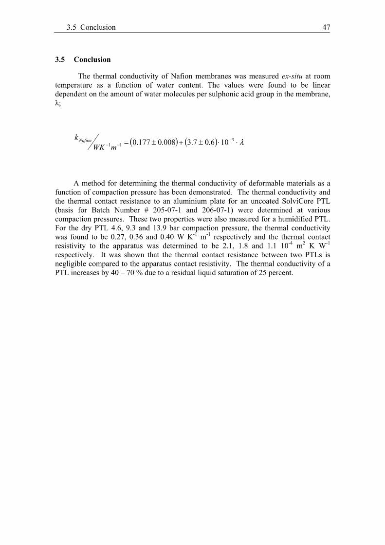
3.5 Conclusion 47
3.5 Conclusion
The thermal conductivity of Nafion membranes was measured ex-situ at room temperature as a function of water content. The values were found to be linear dependent on the amount of water molecules per sulphonic acid group in the membrane, λ;
311 106.07.3008.0177.0
mWKk Nafion
A method for determining the thermal conductivity of deformable materials as a function of compaction pressure has been demonstrated. The thermal conductivity and the thermal contact resistance to an aluminium plate for an uncoated SolviCore PTL (basis for Batch Number # 205-07-1 and 206-07-1) were determined at various compaction pressures. These two properties were also measured for a humidified PTL. For the dry PTL 4.6, 9.3 and 13.9 bar compaction pressure, the thermal conductivity was found to be 0.27, 0.36 and 0.40 W K-1 m-1 respectively and the thermal contact resistivity to the apparatus was determined to be 2.1, 1.8 and 1.1 10-4 m2 K W-1 respectively. It was shown that the thermal contact resistance between two PTLs is negligible compared to the apparatus contact resistivity. The thermal conductivity of a PTL increases by 40 – 70 % due to a residual liquid saturation of 25 percent.


Chapter 4
4 Through-Plane Thermal Conductivity of PEMFC Porous Transport Layers (GDLs)
Odne Burheim, H. Lampert, Preben J. S. Vie, Jon Pharoah and Signe Kjelstrup
Department of Chemistry
Norwegian University of Science and Technology
N-7491 Trondheim, Norway
This chapter is meant to become a short communication to support and supplement Chapter 2 and Chapter 3.

Chapter 4. Through-Plane Thermal Conductivity of PEMFC Porous…
50
ABSTRACT
We report the through-plane thermal conductivities of the several widely used carbon porous transport layers (PTLs or GDLs) and their thermal contact resistivity to an aluminium polarisation plate. We report these values both for wet and dry samples and at different compaction pressures. We show that depending on the type of PTL and possible residual water, the thermal conductivity of the materials differ by an order of magnitude, 0.15 and 1.6 W K-1 m-1 – one order of magnitude in difference. This behaviour is the same for the contact resistivity varying from 0.8 to 11 10-4 m2 K W-1. For dry PTLs the thermal conductivity decreases with increasing PTFE content.
4.1 Introduction
As stated in Chapter 2 and elsewhere [6], [9], the operating PEMFC is not isothermal as it is literally insulated by carbon paper PTLs. In order to achieve efficient control of cooling of fuel cells, knowledge of the through-plane thermal conductivity of these materials is important.
Measurement of the thermal conductivity of PTL materials is complicated for several reasons. A) The in-plane thermal conductivity is very likely to be different from the through-plane [14], [31], B) the through-plane thermal conductivity, the thermal contact resistivity and the thickness changes with the applied compaction pressure [12], C) residual water in the pores significantly changes both the thermal conductivity and the thermal contact resistivity. Therefore care must be taken when measuring the thermal conductivity of PTLs.
Several theoretical approaches have been made to calculate the thermal conductivities of PTL materials. Ramousse et al. [13] estimated minimum and maximum thermal conductivities of carbon papers based on a previously developed model [14], connecting the thermal resistances of the solid and gas phases in parallel series, according to the Maxwell model. Sadeghi et al. [31] developed an analytical model to predict thermal conductivity from the materials structure, simplified by assuming repetitive basic cell contributions.
The first experimental results for the through-plane thermal conductivity were reported by Vie et al. [6], giving a thermal conductivity of 0.19 ± 0.05 W K-1 m-1 for an ETEK ELAT PTL. The experiment was done by inserting thermocouples inside the fuel cell. The relatively large thermocouples increased the uncertainty in the temperature gradient determination for these measurements. Khandelwal et al. [30] reported the first ex-situ measurement on PTL materials, though neither the thermal contact properties to the apparatus nor the in-situ thickness was taken properly into consideration. In addition compaction pressures, likely to severely damage the materials, were applied, i.e. 22 bar. Ramousse et al. [21] used a similar approach. Their apparatus applied copper plates at the end of each cylinder, sandwiching the

4.1 Introduction 51
investigated sample. Using this experimental set-up, different PTL materials provided by Toray (3 different thicknesses) and Sigracet were tested by measuring the thermal resistance on stacks of samples. The PTL bulk through-plane thermal conductivity was estimated based on the assumption that the PTL contact to the apparatus corresponded to a layer as thick as a fibre of 5-10 μm and that the thermal conductivity of this layer would have to be between the values of carbon and air. However, Ramousse et al. did not consider the in-situ thickness at applied compaction pressures. The first experimental report giving all of the three parameters required by Fourier’s law as a function of compaction pressures was Burheim et al. [12]. In addition the contact resistivity towards the apparatus was found properly.
We report here for the first time the through-plane conductivity along with the thermal contact resistivity to a polarisation plate for several different common PTL materials, both dry and humidified, following the procedure described before [12].
4.2 Experimental and modelling
The apparatus [12] was designed to measures the variables that appear in Fourier’s law, i.e. the heat flux, the thickness and the temperature drop over the sample thickness.
The SEM micrographs were obtained using a Hitachi S-3400N ran in SE mode.
Humidifying was done by suction of water through the PTLs during 20 to 30 seconds. The saturation level was obtained by comparing the weight of the PTLs before the measurements to the weight after drying them after the measurements. Each material gave different saturation by this procedure.
In order to better understand some of the aspects of the retrieved data we apply the model described in Chapter 2. The model geometry was shown in Figure 3. Exceptions from the model in Chapter 2 are explained in the section where the model is applied.
4.3 Results
We shall report the through-plane thermal conductivity and thermal contact resistivity of several different dry and wetted PTLs, at different compaction pressures at room temperature. The thermal conductivity was found to change from 0.15 and up to 1.5 W K-1 m-1 depending on water content and applied compaction pressure.
When comparing the different materials, we shall refer to the k/Z-ratio as the ratio of the PTL through-plane thermal conductivity divided by its thickness. This is the inverse thermal resistivity for a given paper and a helpful term as a first-hand evaluation of the materials’ ability to cool the fuel cell.

Chapter 4. Through-Plane Thermal Conductivity of PEMFC Porous… 52
4.3.1 Carbon Papers
In this section we report carbon paper PTLs from three manufacturers; Toray, Sigracet and SolviCore. In general we shall see that adding PTFE to the material will decrease the through-plane thermal conductivity while presence of residual water will increase the through-plane thermal conductivity. We were able to obtain reproducible water content and thus residual water PTL thermal conductivities only for the carbon papers containing non or very little PTFE.
Toray
Toray PTL papers can be delivered in different thicknesses. Some of the bulk properties such as porosity and thermal conductivity depend on this. The material is also available with different PTFE content. The content is indicated by the term “% wet proof”. In this section we will present first the different thickness variations, and next the different “wet proof ability”.
Table 12 gives recorded dimensions and thermal properties of three different Toray TGP-H PTLs, the 060, the 090 and the 120. Comparing the measured results of these, it can be seen that the thermal conductivity increases with increasing PTL thickness. The porosity is approximately the same for the different material classifications. Figure 19 depicts SEM micrographs of the three different classifications. As can be seen, there is very little visual difference between the three pictures. Nevertheless, structural difference must explain the variations in the through-plane thermal conductivity as the porosity is more or less the same for the three different products. At approximately 9 bar compaction pressure the k/Z-ratio of dry 060, 090 and 120 is 3.2, 2.5 and 2.4 kW K-1 m-2. The through-plane thermal conductivity and the contact thermal resistivity increases and decreases with compaction pressure, respectively. This is qualitatively in agreement with previous work [12]. The variation with compaction pressure differs between the three PTL products, however. This further supports the idea of structure variations in Figure 19.
Figure 19 SEM micrographs of PTLs. From left; Toray TGP-H-060, TGP-H-090 and TGP-H-120 – all 5 % wet proof.

4.3 Results and Discussion 53
Table 12 Dimensions and thermal properties of Toray PTL papers at room temperature (5 % wet proof and different thicknesses).
Toray TGP-H-060 (5 % wet proof)
Compaction Dry Residual Water
Pressure / bar
Thickness Z / μm
Porosity ε / %
R’’PTL-Al / 10-4 m2 K W-1
k,PTL / W K-1 m-1
Saturation S / %
R’’PTL-Al / 10-4 m2 K W-1
k,PTL / W K-1 m-1
4.6 172 ± 7 77 ± 1 3.2 ± 0.9 0.41 ± 0.03 68 ± 7 1.2 ± 0.7 1.6 ± 0.3
9.3 165 ± 6 76 ± 1 2.2 ± 0.5 0.53 ± 0.03 71 ± 7 1.0 ± 0.3 1.6 ± 0.2
13.9 159 ± 6 76 ± 1 2.0 ± 0.1 0.66 ± 0.01 75 ± 8 0.8 ± 0.4 1.6 ± 0.2
Toray TGP-H-090 (5 % wet proof)
Dry Residual Water
4.6 275 ± 6 78 ± 1 3.5 ± 0.8 0.50 ± 0.02 61 ± 8 1.2 ± 0.2 1.4 ± 0.1
9.3 265 ± 5 77 ± 1 2.7 ± 0.5 0.65 ± 0.02 71 ± 2 1.3 ± 0.2 1.5 ± 0.1
13.9 256 ± 3 77 ± 1 2.0 ± 0.5 0.73 ± 0.03 70 ± 4 0.7 ± 0.2 1.4 ± 0.1
Toray TGP-H-120 (5 % wet proof)
Dry Residual Water
4.6 345 ± 5 77 ± 1 3.5 ± 0.9 0.62 ± 0.03 31 ± 6 1 ± 2 1.4 ± 0.5
9.3 333 ± 3 76 ± 1 2.6 ± 0.5 0.81 ± 0.03 32 ± 6 0.9 ± 0.8 1.4 ± 0.3
13.9 322 ± 3 75 ± 1 1.9 ± 0.3 0.89 ± 0.02 34 ± 6 0.8 ± 0.4 1.4 ± 0.1
Table 13 shows the through-plane thermal conductivity and resistivity of different wet proof qualities; TGP-H-090, 5, 10 and 60 %. The wet proof quality depends on the PTFE content. SEM micrographs of the three samples are shown in Figure 20. Whereas the thickness is more or less the same for these papers, 250-270 μm, the porosity changes as more Teflon is put into the sample. Teflon and carbon has very similar density (approximately 2.15 g cm-3) and thus the weight and thickness measurement represent the actual porosity to a good approximation. In Figure 20 it can be seen by comparing the micrograph of TGP-H-090 60 % wet proof to the two others that Teflon is highly present. In fact, the amount of PTFE made it difficult to obtain a good picture of this sample. The PTFE content is also reflected in the measured porosity, dropping from around 77 % to 50 %. When comparing the thermal conductivity at 9.3 bar compaction pressure, one can see that it drops with more than 50 %. The 5 % wet proof containing 70 % residual water has a thermal conductivity five times the thermal conductivity of the dry 60 % wet proof.
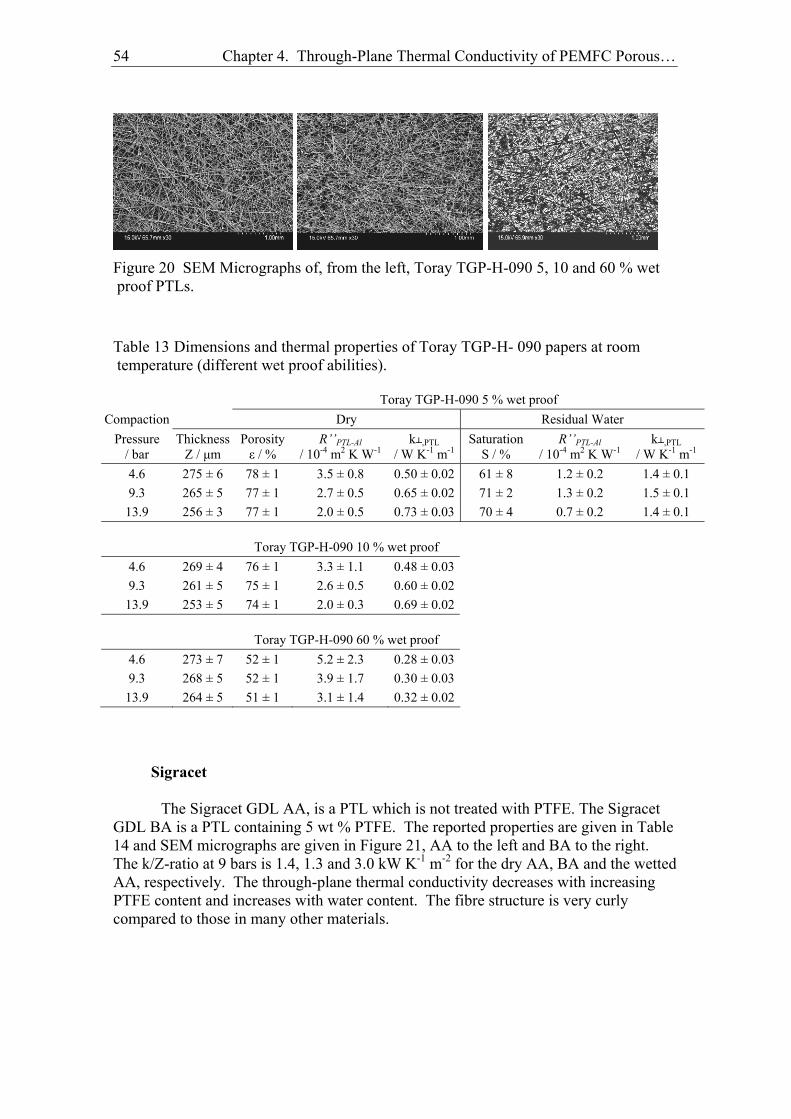
Chapter 4. Through-Plane Thermal Conductivity of PEMFC Porous… 54
Figure 20 SEM Micrographs of, from the left, Toray TGP-H-090 5, 10 and 60 % wet proof PTLs.
Table 13 Dimensions and thermal properties of Toray TGP-H- 090 papers at room temperature (different wet proof abilities).
Toray TGP-H-090 5 % wet proof
Compaction Dry Residual Water
Pressure / bar
Thickness Z / μm
Porosity ε / %
R’’PTL-Al / 10-4 m2 K W-1
k,PTL / W K-1 m-1
Saturation S / %
R’’PTL-Al / 10-4 m2 K W-1
k,PTL / W K-1 m-1
4.6 275 ± 6 78 ± 1 3.5 ± 0.8 0.50 ± 0.02 61 ± 8 1.2 ± 0.2 1.4 ± 0.1
9.3 265 ± 5 77 ± 1 2.7 ± 0.5 0.65 ± 0.02 71 ± 2 1.3 ± 0.2 1.5 ± 0.1
13.9 256 ± 3 77 ± 1 2.0 ± 0.5 0.73 ± 0.03 70 ± 4 0.7 ± 0.2 1.4 ± 0.1
Toray TGP-H-090 10 % wet proof
4.6 269 ± 4 76 ± 1 3.3 ± 1.1 0.48 ± 0.03
9.3 261 ± 5 75 ± 1 2.6 ± 0.5 0.60 ± 0.02
13.9 253 ± 5 74 ± 1 2.0 ± 0.3 0.69 ± 0.02
Toray TGP-H-090 60 % wet proof
4.6 273 ± 7 52 ± 1 5.2 ± 2.3 0.28 ± 0.03
9.3 268 ± 5 52 ± 1 3.9 ± 1.7 0.30 ± 0.03
13.9 264 ± 5 51 ± 1 3.1 ± 1.4 0.32 ± 0.02
Sigracet The Sigracet GDL AA, is a PTL which is not treated with PTFE. The Sigracet
GDL BA is a PTL containing 5 wt % PTFE. The reported properties are given in Table 14 and SEM micrographs are given in Figure 21, AA to the left and BA to the right. The k/Z-ratio at 9 bars is 1.4, 1.3 and 3.0 kW K-1 m-2 for the dry AA, BA and the wetted AA, respectively. The through-plane thermal conductivity decreases with increasing PTFE content and increases with water content. The fibre structure is very curly compared to those in many other materials.

4.3 Results and Discussion 55
Figure 21 A SE SEM micrograph of the Sigracet AA (left) and BA (right) GDLs containing 0 and 5 wt % PTFE, respectively.
Table 14 Dimensions and thermal properties of Sigracet PTL carbon papers.
Sigracet GDL 10 AA
Compaction Dry Residual Water
Pressure / bar
Thickness Z / μm
Porosity ε / %
R’’PTL-Al / 10-4 m2 K W-1
k,PTL / W K-1 m-1
Saturation S / %
R’’PTL-Al / 10-4 m2 K W-1
k,PTL / W K-1 m-1
4.6 301 ± 15 87 ± 1 4.8 ± 1.6 0.30 ± 0.02 66 ± 11 0.3 ± 5.0 0.7 ± 0.3
9.3 275 ± 17 84 ± 2 3.9 ± 1.6 0.38 ± 0.03 72 ± 126 0.5 ± 2.0 0.83 ± 0.14
13.9 246 ± 15 84 ± 2 2.5 ± 1.8 0.42 ± 0.04 83 ± 15 0.6 ± 1.2 0.87 ± 0.10
Sigracet GDL 10 BA
4.6 288 ± 12 85 ± 1 7.2 ± 3.8 0.26 ± 0.03
9.3 244 ± 8 83 ± 1 4.3 ± 2.1 0.30 ± 0.02
13.9 210 ± 6 81 ± 1 3.2 ± 1.8 0.33 ± 0.03
SolviCore
The through-plane thermal conductivities of the SolviCore PTL were previously reported [12]. As water is easy to implement to the material, the PTFE content is most likely very low. The earlier data are repeated here in order to ease the comparison to the rest of the presented material data, see Table 15. The fibres are straight, as can be seen from the micrograph in Figure 22. The thermal conductivity increases with increasing compaction pressure and increasing water content. The k/Z-ratio at 9.3 bar is approximately 1.3 kW K-1 m-2. Even though the SolviCore PTL and the Sigracet PTLs have very different carbon fibre structures their through-plane thermal conductivities are behave similarly. Predictions obtained from a model of Danes and Bardon, give that fibre curvature structure differences, such as present in the SolviCore and the Sigracet PTLs, lead to through-plane thermal conductivity variations of a factor six (e.g. 0.2 and 1.4) [13].

Chapter 4. Through-Plane Thermal Conductivity of PEMFC Porous… 56
Table 15 Thermal conductivities of the SolviCore PTL. [12]
SolviCore PTL
Compaction Dry Residual Water
Pressure / bar
Thickness Z / μm
Porosity ε / %
R’’PTL-Al / 10-4 m2 K W-1
k,PTL / W K-1 m-1
Saturation S / %
R’’PTL-Al / 10-4 m2 K W-1
k,PTL / W K-1 m-1
4.6 221 – 309 83 ± 2 2.1 ± 0.6 0.27 ± 0.03 24 ± 3 0.98 ± 0.7 0.45 ± 0.01
9.3 215 – 295 83 ± 2 1.8 ± 0.8 0.36 ± 0.08 25 ± 3 0.7 ± 0.5 0.54 ± 0.03
13.9 206 – 285 83 ± 2 1.1 ± 0.3 0.40 ± 0.04 26 ± 3 0.5 ± 0.7 0.57 ± 0.06
Figure 22 A SEM micrograph SolviCore PTL untreated carbon paper.
4.3.2 Carbon felts
The carbon felts are again different from carbon papers. They are very soft and can be bent and curled without fracturing. Another difference, it seems, is the perceptibility for water. We were not able to saturate these materials in the manner which we did with some of the carbon papers.
E-TEK
A classical PTL material used for so many fuel cell experiments is the E-TEK carbon felt. Its thermal conductivity vary little with change in compaction pressure though the thickness does and thus the k/Z-ratio, which is 1.3, 1.6 and 1.9 for 4.6, 9.3 and 13.9 bars, respectively. This can be seen in Table 16. A SEM micrograph is given in Figure 23, showing the well known woven structure of the E-TEK carbon cloth.

4.3 Results and Discussion 57
Table 16 Dimensions and thermal properties of the E-TEK PTL carbon cloth.
Compaction E-TEK EC-CC1-060
Pressure / bar
ThicknessZ / μm
Porosity ε / %
R’’PTL-Al / 10-4 m2 K W-1
k,PTL / W K-1 m-1
4.6 211 ± 9 72 ± 1 5.2 ± 2.3 0.28 ± 0.03
9.3 184 ± 11 69 ± 1 3.9 ± 1.7 0.30 ± 0.03
13.9 170 ± 11 66 ± 1 3.1 ± 1.4 0.32 ± 0.02
Figure 23 A SEM micrograph of the E-TEK EC-CC1-060.
Freudenberg FFCT
The Freudenberg H2315 is a carbon cloth which comes with and without additional PTFE. The fibre structure is similar to the one of the Sigracet, as can be seen in Figure 24. Except from the smaller porosity the PTFE treatment introduces no other difference, as can be seen from Table 17. This is also the material with the lowest measured through-plane thermal conductivity among the materials presented in this report. The k/Z-ratio is 0.8 kW K-1 m-1, which is the lowest value found in this study.
Table 17 Dimensions and thermal properties of Freudenberg PTL carbon Cloth
H2315 H2315 T10A (PTFE 10 wt %)
Compaction Pressure
/ bar
Thickness Z / μm
Porosity ε / %
R’’PTL-Al / 10-4 m2 K W-1
k,PTL / W K-1 m-1
ThicknessZ / μm
Porosity ε / %
R’’PTL-Al / 10-4 m2 K W-1
k,PTL / W K-1 m-1
4.6 190 ± 3 75 ± 1 11.1 ± 5.5 0.14 ± 0.02 184 ± 6 72 ± 1 7.8 ± 2.1 0.15 ± 0.01
9.3 182 ± 2 74 ± 1 8.8 ± 4.6 0.15 ± 0.02 175 ± 5 71 ± 1 6.2 ± 2.1 0.15 ± 0.01
13.9 177 ± 2 70 ± 1 7.9 ± 4.0 0.15 ± 0.02 170 ± 5 70 ± 1 4.9 ± 1.5. 0.16 ± 0.01

Chapter 4. Through-Plane Thermal Conductivity of PEMFC Porous… 58
Figure 24 A SEM micrograph of the Freudenberg H2315 carbon cloth
4.4 Discussion
Water contribution
The measured results clearly show that the presence of interstitial liquid water increases the through-plane thermal conductivity of the PTL. One question which arise when these results are compared is whether volume averaging of air, water and carbon to a good approximation can estimate the PTL through-plane thermal conductivity. Consider therefore that the dry papers have one contribution from air (kair = 0.025 W K-1 m-1) and another from the carbon structure, kCS. Thus, if a volume average model is applicable, the thermal conductivity of a PTL with residual water should be equal to the sum of the thermal conductivities multiplied by their respective volume fractions, as suggested in Eq. 4.1. s is the saturation (vol % of pores filled with water) and ε is the porosity (vol % not being solid), so that the equation applies also to the dry PTLs when s equals zero.
Because we have measured the through-plane thermal conductivities of both dry PTLs and PTLs with residual water, this study gives a unique opportunity to test the postulate that volume fraction of air, carbon structure and water can be applied to estimate the through-plane thermal conductivity for PTLs containing liquid water. The answer here seems to depend on the materials; maybe yes for the Sigracet and the SolviCore PTLs and no for the Toray PTLs. This is shown in Table 18. The estimated value based on the volume average model seems to always under-predict the measured values. This suggests that water improves the thermal contact between the fibres rather than a random improvement. This is a question which indeed is important to FC modellers. Several papers show that water tends to cluster and only be present in liquid form at different regions in the fuel cells [22], [23], [25], typically under the ribs next to the flow fields. Thus, at least for the SolviCore and the Sigracet, different PTL thermal conductivities can be estimated at different regions in the cell.
, 1 1100 100 100 100 100PTL Water CS Air
s sk k k
k
(4.1)

4.3 Results and Discussion 59
Table 18 Volume fraction estimates of the through-plane thermal conductivity of dry and partly humidified PTLs.
Sample
ε
/ %
Measured kPTL dry /
W K-1 m-1
kCS / W K-1 m-1
s / %
Predicted kPTL+W /
W K-1 m-1
Measured kPTL+W /
W K-1 m-1
Maximal Prediction kPTL+W /
W K-1 m-1
Toray TGP-H 060 76 0.53 2.13 71 0.83 1.6 0.95
Toray TGP-H 090 77 0.65 2.75 71 0.95 1.5 1.08
Toray TGP-H 120 76 0.81 3.30 32 0.95 1.4 1.23
SolviCore PTL 83 0.36 2.00 25 0.48 0.54 0.82
Sigracet GDL AA 84 0.38 2.25 72 0.72 0.83 0.85
Fibre structure and Teflon content
When comparing the Sigracet AA PTL, the Sigracet BA PTL and the SolviCore PTL, it is clear that the fibre structure in the papers is not necessarily the most important factor for the through-plane thermal conductivity. Adding 5 wt% PTFE to the Sigracet AA paper impairs the thermal conductivity of the material, while straightening out the fibres have apparently little or no effect for the through-plane thermal conductivity as predicted by others [13], [14]. This raises questions around the mechanisms for heat conduction in PTL materials. There is little doubt that one of the most important routes for the heat transport is via the fibre to fibre contact. From the SEM micrographs, one can see that the material with the highest conductivity is the one with the least visible fibre to fibre binder, see Figure 19. In addition, this material is the one in this study with the highest porosity. Its thermal conductivity is lowered by approximately a factor two when adding large amounts of Teflon. This is also the material were the impact of residual liquid water is the strongest and for which the volume fraction average model under-predicts the thermal conductivity the most. The measured thermal conductivity was 50-100 % larger than the ones predicted from Eq. 4.1. The increase in the thermal conductivity that water imposes is enormous. Thus one recipe to high thermal conductivity is less binder (stronger fibre to fibre contact) and interstitial water (to increase the fibre to fibre contact region).
Thermal conductivity and thickness
One of the parameters frequently used in the result section of this chapter is the ratio between the thickness and the through-plane thermal conductivity of a PTL. The k/Z ratio gives a fair comparison between the materials’ ability to cool the fuel cell in the 1D perspective, the region under the land. The results in Table 19 show this. The heat produced under the channel is conducted via the in-plane route in the PTL and therefore; decreasing the thickness may not be such a good idea after all. We shall now play with the simple 2D model from Chapter 2, using the parallel flow channel imposed
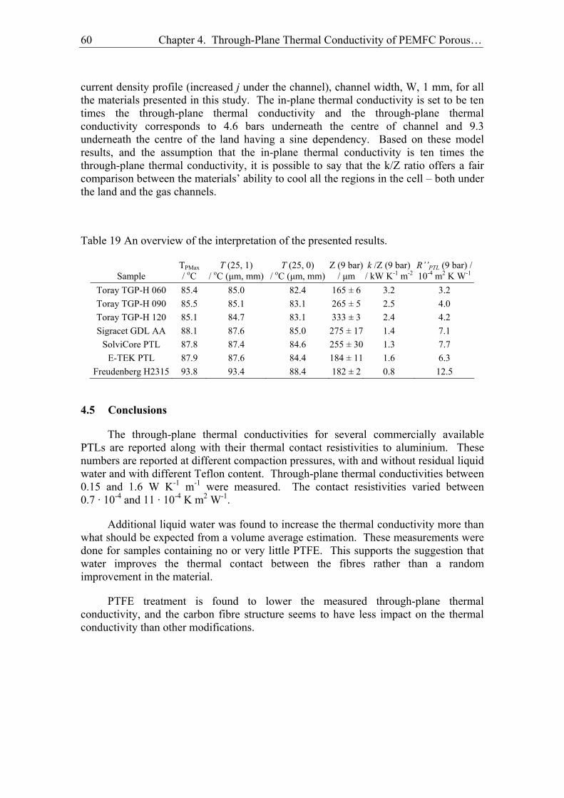
Chapter 4. Through-Plane Thermal Conductivity of PEMFC Porous…
60
current density profile (increased j under the channel), channel width, W, 1 mm, for all the materials presented in this study. The in-plane thermal conductivity is set to be ten times the through-plane thermal conductivity and the through-plane thermal conductivity corresponds to 4.6 bars underneath the centre of channel and 9.3 underneath the centre of the land having a sine dependency. Based on these model results, and the assumption that the in-plane thermal conductivity is ten times the through-plane thermal conductivity, it is possible to say that the k/Z ratio offers a fair comparison between the materials’ ability to cool all the regions in the cell – both under the land and the gas channels.
Table 19 An overview of the interpretation of the presented results.
Sample
TPMax / oC
T (25, 1) / oC (μm, mm)
T (25, 0) / oC (μm, mm)
Z (9 bar)/ μm
k /Z (9 bar) / kW K-1 m-2
R’’PTL (9 bar) / 10-4 m2 K W-1
Toray TGP-H 060 85.4 85.0 82.4 165 ± 6 3.2 3.2
Toray TGP-H 090 85.5 85.1 83.1 265 ± 5 2.5 4.0
Toray TGP-H 120 85.1 84.7 83.1 333 ± 3 2.4 4.2
Sigracet GDL AA 88.1 87.6 85.0 275 ± 17 1.4 7.1
SolviCore PTL 87.8 87.4 84.6 255 ± 30 1.3 7.7
E-TEK PTL 87.9 87.6 84.4 184 ± 11 1.6 6.3
Freudenberg H2315 93.8 93.4 88.4 182 ± 2 0.8 12.5
4.5 Conclusions
The through-plane thermal conductivities for several commercially available PTLs are reported along with their thermal contact resistivities to aluminium. These numbers are reported at different compaction pressures, with and without residual liquid water and with different Teflon content. Through-plane thermal conductivities between 0.15 and 1.6 W K-1 m-1 were measured. The contact resistivities varied between 0.7 · 10-4 and 11 · 10-4 K m2 W-1.
Additional liquid water was found to increase the thermal conductivity more than what should be expected from a volume average estimation. These measurements were done for samples containing no or very little PTFE. This supports the suggestion that water improves the thermal contact between the fibres rather than a random improvement in the material.
PTFE treatment is found to lower the measured through-plane thermal conductivity, and the carbon fibre structure seems to have less impact on the thermal conductivity than other modifications.

Chapter 5
5 A calorimetric analysis of a polymer electrolyte fuel cell and the production of H2O2 at the cathode
Odne Burheim, Preben J. S. Vie, Steffen Møller-Holst, Jon Pharoah
and Signe Kjelstrup
Department of Chemistry
Norwegian University of Science and Technology
N-7491 Trondheim, Norway
This manuscript has been published:
Electrochimica Acta, doi:10.1016/j.electacta.2009.09.053

Chapter 5. A calorimetric analysis of a polymer electrolyte fuel cell and…
62
ABSTRACT
A calorimeter has been constructed and used to measure the total heat production of a single polymer electrolyte fuel cell that is operated on hydrogen and oxygen at 50 °C and 1 bar. The cell had a SolviCore Catalyst Coated Backing and Nafion membranes 112,115 and 117. We report that the total heat production plus the power production corresponds to the enthalpy of formation of water for cell potentials above 0.55 V. For cell potentials less than 0.55 V, we measured a linear decrease in the reaction enthalpy with decreasing cell potential. This effect was obtained independently of membrane thickness and current density. We propose therefore that the main power loss at low cell potentials and the inflection point in the polarisation curve is due to hydrogen peroxide formation at the cathode. The total heat production was decomposed into reversible and irreversible effects (non-ohmic and ohmic). The result was evaluated using Tafel plots. We show that it is possible to determine the overpotential of an electrode also from its thermal signature.
5.1 Introduction
The energy that is dissipated as heat in fuel cells is interesting for several reasons. It provides information that is important for design of auxiliary systems; in particular the cooling systems. Knowledge of the dissipated energy can also help explain the causes of these losses [26]. These issues are now getting increased attention [40], [41], and has motivated us to build a calorimeter and measure the thermal signature of the low temperature polymer electrolyte fuel cell. This paper reports on the construction, test and use of a new calorimeter, as announced earlier [8].
We present a first set of direct calorimetric measurements on a single polymer electrolyte fuel cell, PEMFC, aimed to give direct information of the thermal effects in the cell. To our knowledge, no measurements have so far been reported to access directly the heat produced by fuel cells. The thermal signature was however measured in Li-batteries where possibilities of overheating are large upon discharging as well as charging of the battery [42], [43], [44], [45]. The heat production was measured by placing the battery inside a calorimeter [44], [45]. In the present work, the calorimeter has been tailored to fit around a single cell. The cell has a cylindrical membrane-electrode assembly, and is studied at stationary state. In addition to the heat production, we measure also the simultaneous electric current, the total electric resistance of the cell, and the cell potential.
The cell power can be found from the polarisation curve. By measuring also the heat production, one may add the two values and find the total energy production as a function of current density. If the reactant and product states are the same during the operation, the sum is a constant, as is well known. The characteristic shape of the polarisation curve can be related to the dissipation of energy or the entropy production

5.1 Introduction 63
in the cell. The rapid non-linear fall at relatively low current densities in this curve has thus been attributed to the overpotential, mainly of the oxygen electrode. The linear variation in the potential, E, with current density at intermediated values of the current density is called the ohmic regime. In this regime, the ohmic dissipation explains the variation in the curve. The fall beyond this regime at very high current densities (low cell potentials) has often been attributed to mass transfer limitations [46]. In a simplified calculation of the entropy production, Kjelstrup and Røsjorde [26] found that the non-linear variation in the membrane resistance with water content was essential for the rapid decline. We shall see in this work, that yet another explanation is possible, because the sum of the power production and the heat production can not be explained by the enthalpy of formation of water in the low potential region. Another aim of the work is to find the overpotential, not only from the polarisation curve, but also from its thermal signature. This can be found, as we shall see below, by subtracting the reversible heat and the Joule heat from the total heat production.
In the present set of experiments, a standard membrane (Nafion 112, 115 or 117) and gas diffusion layers, coated with micro porous layers and catalyst (SolvicCore Batch-Number: # 205-07-1, loaded with 0.4 mg Pt cm-2) were chosen, in order to establish results that can be used as reference for later experiments. The cell reaction of the polymer electrolyte fuel cell at the operating conditions in question here (50 °C and 1 bar) can be written as:
(2 2 22 ( ) ( ) 2 ( )H g O g H O l+
2+
2 2+
5a)
Water leaves the cell in the liquid state at these conditions. The electro-osmotic transport of water from the anode to the cathode side, gives a contribution to the cell potential in the mV range. This contribution shall be neglected.
Kinoshita et al. [47] proposed that reduction of oxygen gas proceeds via two parallel pathways, see also Okada and Kaneko [48]. The most important is a direct 4-electron pathway with E 0= 1.23 V,
2 ( ) 4 4 2 ( )O g H e H O l+ + (5b)
The four-electron transfer step was supported by Kuhn et al. [49]. The alternative, undesirable path is a two step pathway via peroxide. The first step is:
2 ( ) 2 2 ( )O g H e H O l+ + (5c)

Chapter 5. A calorimetric analysis of a polymer electrolyte fuel cell and… 64
while the next step c) is:
2 2 2( ) 2 2 2 ( )H O l H e H O l+ + +
2 ( ) 2 ( ) ( )H O l H O l O g+
(5d)
In view of the high half cell potential, an alternative decomposition of peroxide into water and oxygen is likely, with ΔGo and ΔHo equal to -98 kJ mol-1
H2O and -117 kJ mol-1
H2O respectively:
2 2 2 2 (5e)
Whether the oxygen reduction proceeds via path (5b) or paths (5c + 5d) or (5c + 5e) is still a matter of debate among electrochemists [47], [48], [49]. Water formation is thermodynamically favoured, but peroxide production may take place for kinetic reasons. Because hydrogen peroxide formation only requires two electrons transferred it can be kinetically favoured over water formation, requiring four electrons.
Paths (5b) and (5c + 5d) involve the same beginning and end states, defined by the enthalpy of formation of water. Path (5c + 5e), however, is not parallel to step (5b) in the sense that this path gives a different end state from the two first paths. The sum of the heat and power production in the cell is therefore expected to change if there is a crossover from path (5c + 5e) to the other paths. The Tafel slopes for path (5b) or (5c + 5d) have been reported as 2.3 RT / F, i.e. α = 0.43 [48].
Yamanaka has shown that a polymer electrolyte fuel cell can produce hydrogen peroxide [50]. The cathode of his cell was fed with oxygen in the water phase while the anode was in contact with hydrogen gas. Maximum concentrations of peroxide (up to 7 wt%) were obtained under short circuit conditions with heat treated, carbon-containing catalysts in NaOH. Although the yield of water from oxygen reduction is normally more than 98% on Pt, peroxide production was shown to occur below 0.3 V vs. the standard hydrogen electrode [48]. In an evaluation of the cell’s heat and power production, peroxide formation at low potentials is therefore a possibility. We report measurements that allow us to evaluate this from the perspective of combined calorimetric and potential measurements.
We shall thus report on the total heat production and the simultaneous power production in this cell and evaluate the combination. We shall find the separate contributions to the heat production as mentioned above, using the ohmic resistance, the cell potential and the electric current in the cell under operation. This allows us to

5.1 Introduction
65
H U p V q nE F
q T S
answer the following questions: Which reaction mechanism is supported by the experimental data? Which overpotential can be calculated from the total heat production, and how does this calculation compare to the standard determination of the overpotential? Answers to these questions may add insight into the cause of the overpotential. They may also be important, not only for fuel cell modelling, but also for analysis of electrochemical cells where heat effects are important, like Li-batteries.
We shall first see that we have been able to establish a reliable measuring technique, and that we can use this technique to evaluate the electrode reactions. We shall next see that it is possible to find the overpotential also via its thermal signature, with fair precision. The outline of the paper is as follows. We give first an overall thermodynamic analysis of the single polymer electrolyte fuel cell, when placed in a calorimeter at steady state (section 5.2). We describe next a first generation calorimeter used to measure the described effects (section 5.3.1), and the experimental procedure used (sections 5.3.2 and 5.3.3). The results are then presented and discussed in section 5.4.
5.2 Theory
Consider first the cell at temperature T under reversible conditions. There is a change in internal energy, ΔU, when heat is added to the cell and work is done by the cell. The pressure, p, is constant, and ΔV is the volume change by the reaction. The electric work per mole of charges passing the cell is FErev. The first law of thermodynamics gives
rev rev (5.1)
Here F is Faraday's constant and n is the number of electrons transferred in the cell reaction. The heat delivered to the cell under reversible conditions is qrev, and from the definition of entropy we have
(rev 5.2)
where S is the entropy and Δ refers to the cell reaction. The heat change in the surroundings at reversible conditions equals

Chapter 5. A calorimetric analysis of a polymer electrolyte fuel cell and… 66
(surr revq q T S
nE F G T S H
E E Rj
5.3)
This makes the entropy change in the reversible fuel cell plus its nearest surroundings equal to zero, in agreement with the second law. In this particular fuel cell, ΔS is negative and relatively large, since water is formed in the liquid state and gas molecules disappear, cf. (5a). Therefore, the reversible heat effect in the surroundings is positive. Other electrochemical cells may have a cell reaction with a positive entropy change. Such cells can convert heat directly to electric work by taking heat from the surroundings, see [51].
By introducing Eq. 5.2 and the definition of Gibbs energy, G, into Eq. 5.1 we obtain the Nernst equation:
(rev 5.4)
For reversible conditions, Erev = - ΔG/nF. The theoretical value of Erev is 1.21 V at T = 298 K when water is in the liquid state and the reactants are at 1 bar [52]. The negative reaction entropy contributes by -0.25 V and ETN = ΔH/nF by 1.48 V at T = 298 K. So already for very small current densities, the heat production in the cell is substantial. Away from reversible conditions, where there is a net current, the heat production and the entropy production increases [8], [26].
The polarisation curve, where the potential Ecell is plotted as a function of the current density, j, is used to describe the cell’s performance. The current density is the electric current per unit area. As the current density increases, the heat production increases relatively more. We shall use conditions that give small diffusion limitations in the electrodes. The potential of a cell in operation, Ecell, is then the reversible potential minus the ohmic potential drop, Rj, minus the self values of the reaction overpotentials of the overpotentials at the cathode and the anode, η [46]. Here R is the ohmic resistance of the total cell.
cell rev (5.5)
The ohmic potential drop and the overpotential give irreversible heat production (entropy production). These well known thermodynamic relations for an electrochemical cell are illustrated in Figure 25. The overpotential can be described by the Butler-Volmer equation for small current densities and by the Tafel equation for

5.2 Theory 67
larger ones. The overpotential is zero when j = 0. When j → 0, we obtain the Nernst equation, Eq. 5.4.
The power production of the cell (in W per unit of membrane area) is
2cell
H T SP E j j j j R
nF
(5.6)
The total heat production by the fuel cell becomes:
2Q j jnF
T S
Rj
(5.7)
The sum of the power production and the heat production (in J per unit of membrane area) is therefore:
surrTNE j P Q j P j
nF F
qH (5.8)
The sum is called the thermo-neutral power of the cell. It is a hypothetical power.
The heat effects that make qsurr different from –qrev in Eq. 5.3 are due to the overpotential and the Joule heat under the current approximations. These heat effects in Eq. 5.7 are the entropy production [8], [26]. The heat production of the irreversible system is larger than of the reversible one, which it should be, according to the second law. The Joule heat term varies quadratically with the current density, as Rj². The non-ohmic heat effect, the last term on the right hand side of Eq. 5.7, is a heat source which varies non-linearly in j because the overpotential is a strong function of ln j.

Chapter 5. A calorimetric analysis of a polymer electrolyte fuel cell and… 68
TΔS/nF
cell
Figure 25 Thermodynamic properties of an electrochemical cell. The thermoneutral potential in kJ/mol is represented by -ΔH. Part of this energy is needed to compensate the entropy change ΔS at temperature T, leaving us with -ΔG, available for electric work at reversible conditions, Erev. The electric potential under operation is Ecell. Parts of Erev (in V) are used to compensate the overpotential (η) and the Ohmic potential drop (jR).
The overpotentials of the electrodes are here both represented by one symbol η. This is possible if they have the same mathematical form. We can assume that the overpotential of the hydrogen electrode is small, and that the overpotential then represents the oxygen electrode overpotential. Above 0.3 V for the single reaction, the overpotential follows the Tafel equation
η = (RT/αF) ln j/jo (5.9)
or
lna b j (5.10)
where a = - (RT/αF) ln jo and b = RT/ αF. Here jo is the exchange current density of the cathode, and α is the transfer coefficient for the overall reaction of the electrode, while a and b are coefficients from a linear fit of data. When we introduce this expression for the overpotential into Eq. 5.6, the power becomes a non-linear function of the current density.
The purpose of this work is twofold. We want to determine the sum of P and Q in Eq. 5.8, and compare this value to ΔHj/nF for the normal cell reaction (5a). We also want to calculate the overpotential using Eq. 5.7 from the total heat production by the fuel cell in the surroundings, Q, the entropy change of the cell, and the measured total

5.2 Theory
69
resistance and electric current density. We shall see that we can recover ΔHj/nF for reaction (5a), but only for cell potentials above 0.55 V. For lower cell potentials, we find a systematic deviation from this value. This supports that the product states are different from those given by (5b) or (5c + 5d). In the regime where the experimental value for ΔHj/nF corresponds to the result of these paths, the Tafel plot from the thermal signature and from the polarisation curve become the same within the accuracies of the calculations.
5.3 Experimental
5.3.1 Apparatus
We report an isothermal calorimeter designed to measure the heat production of a fuel cell. The calorimeter is equipped to measure also the cell potential drop, and the cell electric resistance. The calorimeter was constructed as a cylinder with insulated walls, and with heat transport in the axial directions. A cross section through the axis of the cylinder is sketched in Figure 26. The cylinder was insulated on the outside by a layer of expanded polyester (not shown).
Figure 26 A sketch of the cylindrical calorimeter, cutting through the axis of the cylinder. Potential differences, E1 and E2, and the fuel cell potential, EFC, were continuously measured, along with the four temperatures, Tj,i. A denotes anode, C denotes cathode, i means inside and o means outside. The two inner temperatures were read to control the heaters. Gases were fed to the cell though the sides (see arrows), and were leaving the cell along the central axis, after passing the gas flow channels.

Chapter 5. A calorimetric analysis of a polymer electrolyte fuel cell and… 70
Three materials were chosen for the construction. They were PEEK (Poly Ether Ether Ketone), copper and steel (ss316). PEEK was chosen as housing material (see Figure 26), because it is a good thermal and electrical insulator, and easy to machine. It was also the mechanically strongest polymer available. Due to high thermal conductivity, copper was used in the end plates and in two internal heaters (see Figure 26) where uniform temperature was required. Stainless steel was used in the polarisation plates next to the membrane-electrode-assembly, MEA, and in the tubes between the heaters and the end plates, where intermediate thermal conductivity was needed. The calorimeter was made symmetric in two pieces, sandwiching the fuel cell and its radial gas seals. It can thus be used to distinguish between heat leaving the cell on the cathode side and on the anode side. The material dimensions were determined using the computational software COMSOL 3.3. By modelling the heat flows from a central source in a suitably constructed grid, we found a suitable length for the steel cylinders between the central heaters and the end plates.
The stainless steel polarisation plate was 11 mm thick. A serpentine flow field (depth, land and channel width equal to 1 mm) was carved into the side next to the fuel cell. Hydrogen and oxygen were fed into the channels via inlets next to the polar plates, see arrows for each gas inlet in Figure 26. Exhaust gases left the calorimeter through the central axis, as shown in the figure.
The heaters consisted of two copper disks, four and six mm thick, and a resistive heating wire, 10 Ω. The heating wire was laid into a channel which was carved into the thicker copper plate. The channel was two mm deep and two mm broad. By inserting two small K-type thermocouples into holes (diameter 0.7 mm) in the thin disk, we measured and controlled the temperatures of the doubly layered copper heaters. The planar copper surface facing the fuel cell was sealed from the PEEK housing by an O-ring, in a 0.5 mm deep channel in the PEEK. The sealing avoided gas leakage along the walls between the PEEK and the steel cylinder.
The purpose of the steel cylinders were to thermally insulate the copper end plate from the double layered heating plate, so that a significant temperature gradient would sustain throughout experiments at all cell operating conditions and at the same time collect the electric current.
Copper plates were used at the end of the steel cylinders. These end plates were cooled to constant temperature by circulating cold water through copper pipes, soldered onto the plate.
The apparatus allowed us to measure the local temperature at several positions. Potential differences were also measured. The fuel cell potential was measured between the gas flow channel plates. All thermodynamic data in Eqs. 5.7 and 5.8 therefore refer to the polar plate positions. All parameters were surveyed and logged by a LabView setup. This includes the load (Agilent 6060B), the power supply (Agilent EE3633A), the High Frequency Ohmeter (HFO) (Agilent 4338B) and the gas flow meters (Burkert, CMOSensTM). In fact, the LabView setup controlled all parts of the operating system

5.3 Experimental 71
except the heaters in the two copper heaters, the cooling water and the humidification. These were controlled by Eurotherm PID-controllers, a refrigerated water bath and by bubbling feed gases through thermostatted water.
The fuel cell was put between the mirror symmetric heaters. The fuel cell consisted of a Nafion 112, 115 or 117 membrane sandwiched between pre-made sheets consisting of catalyst layer, micro porous layer and porous transport layer (these three sections were assembled to the SolviCore Catalyst Coated Backing, Batch Number # 205-07-1, loaded with 0.4 mg Pt cm-2). The active area was 10.2 cm2. The catalyst and catalyst backing were always the same.
The feed gases were humidified by bubbling them through water at 313 K. The humidifiers consisted of a cylindrical closed water bath, where the gases were bubbled through a porous plug close to the bottom. The humidifiers, containing magnetic stirrers, stood upon a plate which controlled the temperature inside the humidifiers. The stoichiometric flow rates where 1.5 for the hydrogen and 3 for the oxygen. The gases were pure thereby eliminating possible mass transfer limitations to the cell membrane.
5.3.2 Measurement
Each experiment started by conditioning the cell. This was done by alternating the cell potential, Ecell, between 0.70 and 0.20 V, keeping the voltage ten minutes at each level, until the current responses were reproducible. The procedure was repeated after the experiment to make sure that the cell performance was the same after as before the experiment.
Polarisation curves were next obtained, keeping a constant cell potential, Ecell, for one hour at every potential, changing the value in steps of 50 mV from 0.2 V up to OCP. At all currents, the power to the heaters were measured, Qheaters,j. The first ten minutes of every step was discarded as the PID controllers required time to adapt to new conditions. To monitor possible ohmic heating in the housing, the potential drops were logged across these regions as well. These potential differences are denoted E1 and E2
in Figure 26, and represents, along with the total electric current, the resistances R1 and R2, respectively The cell resistance is obtained by subtracting these resistances from the overall resistance measured with the Agilent high frequency ohmmeter.
The total heat production by the fuel cell was found as the heat production, Qheaters,j=0, in excess of the heat produced by the heating elements, Qheaters,j, corrected for the cooling of the cell by the feed gases, Qgas, and the ohmic heating in the cell house. Whenever the fuel cell is giving off very little heat, the values of Qheaters,j=0 and Qheaters,j are similar, and the accuracy in the determination of the difference goes down. Qgas was found as a function of the controlled gas stream velocities by calibration with the fuel cell at open circuit. Qhouse is equal to the potential drop in the house multiplied by the total current for the running cell.

Chapter 5. A calorimetric analysis of a polymer electrolyte fuel cell and… 72
(5.11)
, 0 , heaters j heaters j gas house ohmicQ Q Q Q Q
5.3.3 Data reduction procedure
Some of thermodynamic data used in the calculation are shown in Table 20. The entropy change in the cell is equal to:
2 2
00 1/2 0
ln( / ) ( /
w
O H
S S R)
a
p p p pD =D + (5.12)
The water activity a is unity in pure liquid water. The total gas pressure on both
sides is 1 bar. The partial pressures of oxygen and hydrogen are slightly lower than 1 bar, due to the presence of water vapour on both sides. This has a negligible effect on the entropy change (less than 1 % at 323 K), however, leaving us with the standard value.
w
Table 20 Standard state thermodynamic data at 298 K for production of one mole product. [52]
ΔGo
/ kJ mol-1 Eo
/ V ΔHo
/ kJ mol-1 ETN / V
2 2 2
1( ) ( ) ( )
2H g O g H O l
-237
1.23
-286
1.48
2 2 2
1( ) ( ) ( )
2H g O g H O g
-229
1.19
-242
1.25
2 2 2 2( ) ( ) ( )H g O g H O l
-120 / -134*
0.62 / 0.69*
-188 / -191*
0.97 / 0.99*
*Infinitely diluted hydrogen peroxide
Integrating from 298 K to the temperature of operation, 323 K, the entropy of reaction becomes -164 J K-1 mol-1, the enthalpy of reaction is -284 kJ mol-1
H2O, the Gibbs energy change of the reaction is -231 kJ mol-1, and the reversible cell potential is 1.20 V. The products TΔS/nF and ΔH/nF are -0.27 and 1.47 V, respectively at 323 K.
The fuel cell electric power output, P =Ecellj, was calculated from measured cell voltage, Ecell, and the corresponding current density, j = I/A, where I is the electric current (in C/s), and A is the area of the fuel cell membrane. The total energy production, the thermoneutral power, ΔH (j/F), was calculated by introducing values of P and Q into Eq. 5.8.

5.3 Experimental
73
5.4 Results and Discussion
We present and discuss the measured contributions to total energy production in a fuel cell. We demonstrate that the total energy production is reduced at low cell potentials and that the power output from the fuel cell starts to decline simultaneously, and argue that these two trends are related to hydrogen peroxide production. We give also the overpotential of the cell obtained from the thermal signature, and conclude that it compares well to the value obtained from the potential measurements.
5.4.1 The reaction enthalpy
Typical results for heat and power measurements are shown in Fig. 3 for a cell with a Nafion 112 membrane at 323 K and 1 bar. The heat production is shown by square points as a function of current density. The fuel cell power is shown by circular points. The sum of the two gives the total energy production from the fuel cell. We find that the energy production is directly proportional to j until the current density reaches 0.9 A cm-2 in Figure 27. The theoretical value of the thermoneutral potential for production of liquid water, multiplied by the current density, is presented by the stippled line for comparison. We see a perfect agreement with the value for water production up to the given current density. After that, the total energy production falls below the one expected for water as a product.
In order to elucidate this situation further, we plotted the experimental result for the thermoneutral potential (the derivative of the total energy conversion in Figure 27 (triangular points)) as a function of the cell potential in Figure 28. This figure also gives the measured thermoneutral potential from cells using Nafion 115 and 117 membranes. The straight stippled line gives the theoretical value of the thermoneutral potential of formation of liquid water at 323 K, 1.47 V. It is equal to the slope of the stippled line in Figure 27. A very good agreement between experimental and theoretical values is found for cell potentials above 0.55 V. The measurements show larger scatter in the measured thermoneutral potential at lower than at higher current densities. We compare very similar numbers, i.e. Qj=0 vs. Qj≈0 in this region and fluctuations in the PID controllers enhance the error further. The scatter is randomly distributed, however (see also Figure 29a and b). Below a cell potential of 0.55 V, the thermoneutral potential decreases, approximately linearly with the cell potential (Figure 28). The measurement was repeated several times with different membranes in order to make sure that the drop in the thermoneutral potential was not a random error caused by a poor thermal control of the calorimeter, as we believed at first.

Chapter 5. A calorimetric analysis of a polymer electrolyte fuel cell and… 74
0.0
0.3
0.6
0.9
1.2
1.5
1.8
0.0 0.2 0.4 0.6 0.8 1.0 1.2
j / A cm-2
Ene
regy
Pro
duct
ion
/ W c
m-2
Total Energy Conversion
Q
P
Figure 27 The total heat production (squares), the electrical energy production (circles), and the total energy production (triangles) as a function of current density in an oxygen/hydrogen fuel cell at 323 K and with Nafion 112 membrane.
1.30
1.35
1.40
1.45
1.50
1.55
1.60
0.200.300.400.500.600.700.800.90Ecell / V
E T
N /
V
E TNNafion 117Nafion 115Nafion 112
Figure 28 Thermoneutral potential, as functions of the cell potential, Ecell, in a fuel cell operated at 323 K, 1 atm and with oxygen. Results are shown for three Nafion membranes.

5.4 Results and Discussion 75
We may speculate on the origin of this decline. The exhaust gases are kept at 50 oC at the polarisation plate and have this temperature when they are passing the heaters. The gases are fed at a rate proportional to the cell current and with constant humidity, and will thus leave at the same condition. The proportion between water vapour and liquid water is therefore expected to be constant in the experiment. The difference in enthalpy of formation for liquid and gaseous water is equal to the vaporization enthalpy for liquid water. Because water vapour in the product would condense at the gas flow plate, the measured heat from the process will thus relate to reaction 1 in Table 20 in any cases. It is therefore unlikely that the decline in the curve is due to production of water vapour instead of liquid water, which gives a smaller enthalpy of reaction. Given this, we must explain the lowering of the thermoneutral voltage in Figure 28 by another product. Reaction (5c) offers hydrogen peroxide as a possible product. The voltage at which it is produced, 0.55 V, supports the idea that hydrogen peroxide leaves the cell as a product.
In order to further test the hypothesis that hydrogen peroxide is formed, we conducted the same experiments with thicker membranes, Nafion 115 and 117, using the same PTL, MPL electrode materials. Fuel cells with these membranes have a higher resistance, and do therefore produce a smaller current at the same cell potential. The measured resistance for the cells where approximately 0.21, 0.41 and 0.71 ohm cm2, using Nafion 112, 115 and 117 respectively. Vie and Kjelstrup [6] reported 0.31 ohm cm2 for the total cell resistance at 70 oC using Nafion 112. We see that the thermoneutral potential varies essentially in the same way for all membranes. This supports the idea, that the cell potential, rather than the current density is essential for the decline in the thermoneutral potential. A further illustration of this is shown in Table 21. The table shows the current density for the three cells in Fig. 4 when the cell potential is 0.3 V. A factor 2 variation in current density is seen. The thermoneutral potential is the same within the uncertainties, however. We conclude that formation of hydrogen peroxide may explain the deviation from the straight stippled line in Figure 28.
Because energies are additive, the total enthalpy change for reactions 1 and 3 in Table 20 can be written:
2 2
22 2 2 2 2 2
2 2
total
2
TN TN
H Otot H O TN TNH O H O H O H O
H O H O
E EH x H x H x
E E
−= + =
− (5.13)
where xi is the mole fraction of peroxide and water, respectively. The product water mole fraction, xH2O, corresponds to the current efficiency in water production and can be calculated from Eq. 5.13, i.e. at 323K thermoneutral potentials of 1.47, 1.43 and 1.39 correspond to mole fractions of water (xH2O), i.e. current efficiencies, of 1.0, 0.92

Chapter 5. A calorimetric analysis of a polymer electrolyte fuel cell and… 76
and 0.84 respectively. This means that our fuel cell produces more than 16 mol % hydrogen peroxide at the lowest cell potential. The peroxide may be diluted by the water transported along with the protons from the anode, so that the end product has a smaller concentration. The mole fraction calculated for water is equal to the current efficiency for water production, and its value is in agreement with other observations [50], [53], [54], [55].
0.00
0.30
0.60
0.90
1.20
1.50
0.000 0.200 0.400 0.600 0.800 1.000 1.200j / Acm-2
E /
V
0.00
0.30
0.60
P /
W c
m-2
E TNEcellP
a) Nafion 112
0.00
0.30
0.60
0.90
1.20
1.50
0.00 0.20 0.40 0.60 0.80 1.00j / Acm-2
E /
V
0.00
0.30
0.60P
/ W
cm
-2
E TNEcellP
b) Nafion 115
Figure 29 a and b. Thermoneutral voltage (squares), polarisation curve (triangles) and electric power (circles) as functions of current density in a fuel cell operated at 323 K, 1 atm, with oxygen and hydrogen and either Nafion 112 or 115 membranes – a and b respectively.

5.4 Results and Discussion 77
Table 21 Corresponding values of cell potential, current density and thermoneutral potential recorded at 323 K using oxygen and hydrogen at 1 bar with various cell membranes.
Ecell
/ V j / A cm-2 ETN / V
Nafion 112 0.30 1.19 ± 0.10 1.37 ± 0.01
Nafion 115 0.31 0.950 ± 0.001 1.38 ± 0.01
Nafion 117 0.31 0.602 1.40 ± 0.02
The reduction in current efficiency for water production in the present cell can be compared to the anode processes in the chlorine-alkaline electrolysis cell. This is the largest electrochemical industrial process in the world and is therefore very well studied [56]. Oxygen evolution is thermodynamically favoured over chlorine evolution, while chlorine evolution has greater current exchange density and approximately half the Tafel slope of oxygen evolution. Therefore, when the overpotential increases to a significant level, the chlorine current efficiency dominates. A similar behaviour seems to be the case for hydrogen peroxide production vs. water production at low fuel cell potentials [50], [53], [54], [55].
5.4.2 The cell power and the polarisation curve
The results of Figure 28 are further documented in Figure 29a and b, for Nafion 112 and 115, respectively. Both Figure 29a and b show a decline in the measured thermoneutral potential at high current densities, i.e. for cell potentials below 0.55 V. The polarisation curves and the power density as functions of the current density are also given in these figures. The start of the decline in the thermoneutral power coincides with the peak in the power density and the inflection point in the polarisation curve. The regions for reduced thermoneutral potential are painted gray in Figure 29a and b in order to emphasise the relation between the thermoneutral potential reduction, the peak in the power curve and the inflection point in the polarisation curve. The stippled lines in Figure 29a and b is meant to illustrate an idealised situation. Linearization of the polarisation curves for potentials between 0.55 – 0.85 V (where the ohmic behaviour is dominating) is used to demonstrate how the power curves would behave if the polarisation curve did not inflect (both stippled). The point where the power curve peaks and starts to deviate from the idealized (stippled) behaviour systematically related to the reduction of the thermoneutral potential, and thus to the cell potential. Production of hydrogen peroxide leads to a reduction in the electric work, as the reaction Gibbs energy is lowered by approximately a factor two, see Table 20. A decline in the power production, as well as the polarisation curve inflection point, at high current densities is often connected to mass transfer problems, see e.g. [46]. In the present case, where pure humidified gases are fed stoichiometrically, this should not be an issue. If, however, mass transfer limitations occurred for the electrodes, this phenomena should reveal itself at a given current density (mass transfer related) rather

Chapter 5. A calorimetric analysis of a polymer electrolyte fuel cell and… 78
than at a given potential (mechanism related). In addition to this, a diffusion-overpotential should also lead to dissipation of energy and reveal itself as a heat. Such dissipation was not observed here, as the thermoneutral potential then would be constant for all cell potentials. These arguments further supports that the observed decline in the power density and the inflection point on the polarisation curve is related to formation of hydrogen peroxide.
Hydrogen peroxide production is a partial reduction of oxygen, favoured by simpler kinetics, few catalytic sites and high reaction rates, as each oxygen atom only has to exchange two electrons [57]. The catalyst and catalyst backing used here were of a commercial pre-made type. The polarisation curve and the power curve depend on the catalyst and its backing. Peroxide production is unwanted, as it affects the fuel cell life time and leads to detrimental loss in the current efficiency. Knowledge about its production is thus essential for fuel cell construction and operation. The present technique is suited to explain ill performance in a new light.
5.4.3 The overpotential from the polarisation curve and the thermal signature
The data discussed above were further reduced to give the overpotential of the oxygen electrode.
Figure 30 gives the familiar polarisation curve (triangles); the measured cell potential as a function of current density. It is reassuring to see that the polarisation curve extrapolates to a value just below 1 V as is commonly observed in fuel cells. The constant upper limit is again the total energy production, discussed above. We shall now limit the analysis to current densities, where the electrode reaction proceeds via the four electron transfer step, or via two two-electron transfer steps, since we are after the overpotential for a well defined cell reaction.
The overpotential of the oxygen electrodes was therefore calculated from Eq. 5.7 and Eq. 5.11 using data from Figure 30 and plotted in Figure 31. The plot as a function of ln j is done for fuel cell potentials above 0.55 V, as this is the region where we can expect Tafel behaviour for a reaction between two defined states. The contribution from the anode overpotential is normally small [47], and we have assumed that the results reflect the cathode overpotential only. The three terms from which the overpotentials stem, Rj, TΔS/nF and Q/j are also shown in the figure. The fit to the plot of η versus ln j, gave a straight line, Eq. 5.15. The cell resistance was 0.31 ohm cm2.
For comparison, the overpotential was also calculated directly from the cell potential and the ohmic potential drop, which is the classical approach. The result is given by Eq. 0.16. The overpotentials, ηthermal and ηclassic, have dimension V and the current density is in A cm-2. The two values agree within the accuracy given, though the classical approach gives a better precision in the determination. This is again due to the scattered results caused by the PID controllers, as can be seen from Figure 31.

5.4 Results and Discussion 79
0.0
0.2
0.4
0.6
0.8
1.0
1.2
1.4
1.6
1.8
0.00 0.15 0.30 0.45 0.60 0.75 0.90 1.05 1.20
j / A cm-2
Pot
entia
l / V E TN
Ecell
IR cell
Figure 30 The polarisation curve (triangles), the ohmic potential drop (crosses), the measured and theoretical thermo neutral voltages at 323 K (1.47 V) for a fuel cell at 1 bar and 323 K with a Nafion 112 membrane.
-0.35
-0.2
-0.05
0.1
0.25
0.4
0.55
0.7
0.85
1
1.15
-3.0 -2.5 -2.0 -1.5 -1.0 -0.5 0.0
ln j
Pot
entia
l / V
Q / j
η
Rj
TΔS / F
linear fit to η
Figure 31 The overpotential of the electrodes in the fuel cell and its contributions. The fuel cell was operated with oxygen /hydrogen at 323 K and Nafion 112 membrane.

Chapter 5. A calorimetric analysis of a polymer electrolyte fuel cell and…
80
4
0.472 0.007 0.063 0.005 ln ,
5.36 0.02 10 , 0.45 0.04
thermal
o
j A cm V j
j
2
(5.15)
4
0.447 0.002 0.0577 0.0016 ln ,
4.24 0.01 10 , 0.483 0.015
classic
o
2 j A cm V j
j
(5.16)
The transfer coefficient was calculated to 0.45 from the thermal signature and 0.483 from the classical approach. The transfer coefficients can be compared with the value given by Okada and Kaneko [48]. They reported Tafel slopes for path (5b) or (5c + 5d) equal to 2.3 RT / F, or α = 0.43 [48].
The intercepts on the y-axis gave exchange current densities of 5.4 and 4.2 x 10⁻⁴ A cm-2 referred to membrane area, from the two approaches respectively. We did not determine the area of the catalyst, so it is not possible to give absolute exchange current densities.
5.5 Conclusions
One aim of the present work has been to document that the thermal signature of the fuel cell is useful. For this purpose we have constructed a calorimeter that is tailor-made to find the heat production corresponding to a fuel cell power. We report some first results of calorimetric measurements in combination with standard electrochemical measurements, and show that new information can be obtained.
A first set of in situ calorimetric measurements has thus been presented for the single polymer electrolyte fuel cell. We also report a non-ohmic heat production, compatible with Tafel’s equation, an exchange current density of 5.4 x 10⁻⁴ A/cm2
(referred to the membrane area) and a transfer coefficient of 0.45. We have demonstrated for the first time that the electrode overpotential in a cell can be determined via a characteristic heat production.
We have seen that the combined measurements indicate that hydrogen peroxide takes place when the cell voltage falls below 0.55 V. We have demonstrated that this effect partly affects the location of the peak in the power density curve and the inflection point in the polarisation curve. At a cell potential of 0.3 V, the current efficiency for production of water may be as small as 85 %. If this is the sole reason for a deviation observed in the energy production, it represents a more important loss in electric power at high current densities than diffusion limitations do.

6 Conclusions and further work
During this PhD study, several apparatuses and experimental routines have been established and applied to different systems. However, the full potential of the test stations have yet to be reached. This chapter summarises the most important conclusions of my work and, additionally, gives suggestions on how to take further advantage of the laboratory setup.
6.1 Conclusions
An apparatus to ex-situ measure the through-plane thermal conductivity was developed and built and routines for measurements were establishment. One crucial challenge to overcome was to determine the correct thickness for the sample during measurements while another one was to deconvolute the different contact resistances for stacked samples. Both of these challenges were solved successfully. The through-plane thermal conductivity for Nafion was measured as a function of water content at room temperature, λ being the number of water molecules per sulphonic group;
311 106.07.3008.0177.0
mWKk Nafion
It was found that for porous transport layers, PTL, the sample to sample thermal contact resistivity is negligible compared to the sample to apparatus thermal contact resistivity. A small data base of through-plane thermal conductivities and material to aluminium thermal contact resistivities was established for more than ten different commercial PTLs. The values reported correspond to different compaction pressures, Teflon content and residual liquid water in the PTLs. Depending on these conditions, the thermal conductivities and thermal contact resistivities were measured to be in the ranges of 0.15 – 1.6 W K-1 m-1 and 0.7 · 10-4 – 11.1 · 10-4 K m2 W-1, respectively.
A calorimeter was constructed. This had the ability to measure both the heat and the work from the fuel cell at constant pressure at a given temperature. The sum of this work and the heat can be added to the reaction enthalpy for the chemical process. Both the heat from the gases leaving and entering the calorimeter and the heat from ohmic heating in the cell housing was encountered for. It was found that when the cell potential was less than 0.55 V, regardless of conversion rate and membrane thickness, the reaction enthalpy of the PEM fuel cell dropped linearly with the cell potential. Due to the design and operation of the calorimeter, the only explanation for this behaviour is partial production of hydrogen peroxide. At cell potential of 0.30 V the measured reaction enthalpy corresponds to more than 15 mol% hydrogen peroxide. From the measured heat generated when the cell was running at potentials above 0.55 V, it was demonstrated that the Tafel behaviour can be obtained.
A 2D thermal model was developed in order to demonstrate the need and possible use for the through-plane thermal conductivity measurements. The model considers

Chapter 6. Conclusions and further work
82
effects imposed by different 3D designs, such as the gas flow channel pattern. It also considers the choice of feed gases and the phase change of water due to humidification of the feed gases. The model demonstrates that for a single fuel cell at a current density of 1 A cm-2 the membrane and catalyst layer, being literally insulated between two PTLs, can have temperatures between 3 and 15 oC above the end plate temperature. The model also gives some perspectives on how the produced heat is distributed to the anode and the cathode end plates. This information is useful for further use of the calorimeter.
6.2 Further work
My suggestions for further work consist of suggestions on how use the already built apparatuses for fuel cells, fuel cell components and for materials related to other applications. I think in addition to this, new apparatuses can be built with the experience from the work presented here. Here I give some ideas;
Regarding the through-plane thermal conductivity apparatus I consider that the method is established and that it now can be used for validation of new fuel cell materials. I also think that the apparatus can be used for materials for different applications, e.g. vinyl amine membranes for CO2-separation. Chapter 2 and Chapter 3 demonstrate that such a study could reveal important relations between transport of water, heat, CO2 and water content in such a system.
The thesis reports measured through-plane thermal conductivity – not in-plane thermal conductivity. As demonstrated in Chapter 2, greater parts of the produced heat are conducted by this in-plane conductivity. This is an experimental property which is not experimentally verified yet, though it might be the most crucial in order to get an over view of the fuel cell temperature distribution. This research will require development of a new apparatus.
The fraction of hydrogen peroxide in the product from the fuel cell process has, by ex-situ techniques, been shown to depend on the catalyst amount, the cell potential and the water content in the region where the reaction takes place [50], [53], [54], [55], [57]. The effects from using MPLs are not fully understood, though it has been demonstrated that they improve the fuel cell performance in the region where we have measured reduction in the total reaction enthalpy. Therefore I propose to run the calorimeter with fuel cells with and without MPLs.
A question which seems to interest many fuel cell researchers is how the heat is distributed among the electrodes. We have shown that this depends partly on the water phase change and electrode reaction entropy. Even though this is a highly complex question, we now have the opportunity to measure and understand these effects, by combining the 2D thermal model and the calorimeter.
The calorimeter is tailored to accommodate PEM fuel cells and is additionally gas tight. When both of the two suggested calorimetric experiments are done, one can

6.2 Further work 83
also replace the hydrogen gas flow controller with a controller capable of controlling a mixture of liquid methanol and water. We may at this stage hypothesise that the oxygen reduction reaction gives off water and hydrogen peroxide when the cell potential is lowered adequately.


Bibliography
[1] International Energy Agency – IEA, Midterm Oil Marked Report 2007, 2008 and
2009, website, http://omrpublic.iea.org/, (August 2009).
[2] Intergovernmental Panel on Climate Changes – IPCC, http://www.ipcc.ch/,
(August 2009).
[3] The Hydrogen Community website, http://www.hydrogensociety.net/,
(August 2009).
[4] A.M. Svensson, S. Møller-Holst, R. Glöckner, O. Maurstad, Energy, 32 (2007)
437-445.
[5] Fuel Cell Norway ANS, http://www.fuelcell.no/principle_history_eng.htm,
(August 2009)
[6] P. J.S. Vie, S. Kjelstrup, Electrochim. Acta, 49 (2004) 1069-1077.
[7] P. J. S. Vie, Characterisation and Optimisation of the Polymer Electrolyte Fuel Cell,
Dr. thesis, NTNU, Norway, 2002.
[8] S. Møller-Holst, S. Kjelstrup, and P. Vie, The 4th International ASME Conference
on Fuel Cell Science, Engineering and Technology, June 19-20, Irvine, California,
2006.
[9] He, S., Mench, M.M., Tadigadapa, S., 2006, Sensors and Actuators A, 125, 170-177
[10] G. Alberti, M. Casciola, L. Massinelli, B. Bauer, Journal of Membrane Science
185 (2001) 73-81.
[11] F. Bauer, S. Denneler, M. Willert-Porada, J Polym Sci Part B: Polym Phys, 43
(2005) 786-795.
[12] O. Burheim, P.J.S. Vie, J.G. Pharoah,S. Kjelstrup, J. Power Sources, 196 (2010)
249-256.
[13] J. Ramousse, S. Didjierjean, O. Lottin, D. Maillet, Int. J. of Thermal Sciences, 47
(2008) 1-6.
[14] F. Danes, J. Bardon, Revue Generale de Thermique, 36 (1997) 302-311.
[15] J. G. Pharoah, K. Karan, W. Sun, J. Power Sources, 161 (2006) 214-224.
[16] D. Harvey, J. G. Pharoah, K. Karan, J. Power Sources, 179 (2008) 209-219.
[17] M. Reum, S.A. Freunberger, A. Wokaun, and F.N. Büchi, J. Electrochem. Society,
156 (2009) B301-B310.

Bibliography 86
[18] M.J. Lampinen, and M. Fomino, J. Electrochem. Society, 140 (1993) 3537-3546.
[19] T. E. Springer, T. A. Zawodsisnki, Jr., and S. Gottesfeld.. J. Electrochem. Soc.,
138 (1991) 2334-2342.
[20] P.J. Reucroft, D. Rivin, N.S. Schneider, Polymer, 43 (2002) 5157-5161.
[21] J. Ramousse, O. Lottin, S. Didierjean, D. Maillet, J. Power Sources, 192 (2009)
435–441.
[22] A. Turhan, K. Heller, J.S. Brenizer, M.M. Mench, J. Power Sources, 180 (2008)
773–783.
[23] P. Boilat, D. Kramer, B.C. Seyfang, G. Frey, E. Lehmann, G.G. Scherer, A.
Wokaun, Y. Ichikawa, Y, Tasaki, K. Shinora, Electrochemistry Communications,
10 (2008) 546-550.
[24] E. Johannessen, S. Kjelstrup, Chemical Engineering Sci., 60 (2005) 3347-3361.
[25] S.Lister, D. Sinton, N.Djilali, J. Power Sources, 154 (2006) 95-105.
[26] S. Kjelstrup and A. Røsjorde, J. Phys. Chem. B., 109 (2005) 9020-9033.
[27] G. Elert, The Physiscs Hypertextbook, January 2006,
hypertextbook.com/physics/thermal/conduction
[28] E. Birgersson, M. Noponen, M. Vynnycky, J. Electrochem. Soc., 152 (2005)
A1021-A1034.
[29] J. Ihonen, Development of Characterisation Methods for the Components of the
Polymer Electrolyte Fuel Cell. Ph.D.-thesis, Stockholm: Dep. Of Chemical
Engineering and Technology, Applied Electrochemistry, Kungliga Tekniska
Högskolan, 2003.
[30] M. Khandelwal, M. M. Mench, J. Power Sources, 161 (2006) 1106-1115.
[31] E. Sadeghi, M. Bahrami, N. Djilali, J. Power Sources, 179 (2008) 200-208.
[32] Thermophysical Properties Laboratory web-page, Hot Wire Methods for the
Thermal Conductivity Measurement, January 2006,
http://www.tpl.ukf.sk/engl_vers/hot_wire.htm
[33] C.L. Choy, K. W. Kwok, W. P. Leung, F. P. Lau, J. Polymer Sci. Part B: Polymer
Phys, 32 (1994) 1389-1397.
[34] M. Spinnler; Int. J. Heat and Mass Transfer, 47 (2004) 1305-1312.
[35] Boedeker Plastics, Inc., Texas 77984, USA, web-page; www.boedeker.com,
(October 2006).

87
[36] T. A. Zawodzinski, M. Neeman, L. O. Sillerud, S. Gottesfeld, J. Phys. Chem., 95
(1991) 6040-6044.
[37] T. E. Springer, T. A. Zawodzinski, S. Gottesfeld, J. Electrochem. Soc., 138 (1991)
2334 – 2342.
[38] K. K. Pushpa, D. Nandan, R. M. Iyer, J. Chem. Soc., Faraday Trans 1, 84 (1988)
2047-2056.
[39] G. E. P. Box, W. G. Hunter, J. S. Hunter, Statistics for experimenters, John Wiley
& Sons, Inc, 1978.
[40] C.Y. Wang, Chem. Rev., 104 (2004) 4727.
[41] A. Faghri and Z. Guo, Int. J. of Heat and Mass Transfer, 48 (2005) 3891.
[42] K. E. Thomas, C. Bogatu, and J. Newman, J. Electrochem. Soc. 148 (2001)
A570-A575.
[43] K. E. Thomas, J. Newman, J. Power Sources, 119-121 (2003) 844-849.
[44] H. Yang and J. Prakash, J. Electrochem. Soc., 151 (2004) A570-A575.
[45] M.N. Richard and J. R. Dahn, Electrochem. Soc., 146 (6) 2068-2077 (1999).
[46] A.Z. Weber, J. Newman, Chem. Rev., (2004), 4679−4726.
[47] K. Kinoshita, Electrochemical Oxygen Technology, Interscience, New York, 1992
[48] T. Okada, and M. Kaneko, Springer Series in Material Sc. ISBN 978-3-540-
70730-1.
[49] H. Kuhn, A. Wokaun, and G.G. Scherer, Electrochim. Acta, 52 (2007) 2322-2327.
[50] I. Yamanaka, Catal Surv Asia, 12 (2008) 78-87.
[51] K. Hemmes, G.P. Dijkema, H.J. van der Kooi, Russian J. of Electrochem. 40
(2004) 1100.
[52] G. Aylward and T. Findlay, SI Chemical Data, 5th edition, Wiley, New York, 2002.
[53] E. Lobyntseva, T. Kallio, N. Alexeyeva, K. Tammeveski, K. Kontturi,
Electrochimica Acta 52 (2007) 7262–7269.
[54] V.A. Sethuraman, J.W. Weidner, A.T. Haug, M. Pemberton, L.V. Protsailo,
Electrochim. Acta, 54 (2009) 5571–5582.
[55] S.L. Gojkovic’, S. Gupt, R.F. Savinell, Electrochim. Acta, 45 (1999) 889–897.
[56] S. Trasatti, Electrodes of Conductive Metallic Oxides, ISBN 0-444-41912-8,
Elsevier Sci. P. Co., 1980
[57] W. Liu and D. Zuckerbrod, , J. El. Soc., 152 (2005) A1165-A1170.


![Laboratory Investigation and Modelling of the Thermal ...downloads.hindawi.com/journals/geofluids/2019/5121740.pdf · [23] whereas the thermal conductivities of salt solutions are](https://static.fdocuments.in/doc/165x107/5e2ceaa60abfe46e2c6645f5/laboratory-investigation-and-modelling-of-the-thermal-23-whereas-the-thermal.jpg)