Theory of the Josephson Junction Laser

Steven H. Simon1 and Nigel R. Cooper2

1Rudolf Peierls Centre, Oxford University, OX1 3NP, United Kingdom2T.C.M. Group, Cavendish Laboratory, J.J. Thomson Avenue, Cambridge, CB3 0HE, United Kingdom

(Dated: July 11, 2018)

We develop an analytic theory for the recently demonstrated Josephson Junction laser (Science355, 939, 2017). By working in the time-domain representation (rather than the frequency-domain)a single non-linear equation is obtained for the dynamics of the device, which is fully solvable insome regimes of operation. The nonlinear drive is seen to lead to mode-locked output, with a periodset by the round-trip time of the resonant cavity.

The physics of Josephson junctions has been studiedintensely for over half a century[1, 2]. These devicesare fairly unique as the only lossless nonlinear low tem-perature circuit elements[3]. Due to interest in usingJosephson physics for quantum computing applications,enormous attention has focused on the combination ofJosephson junctions and low loss resonant cavities[4, 5].

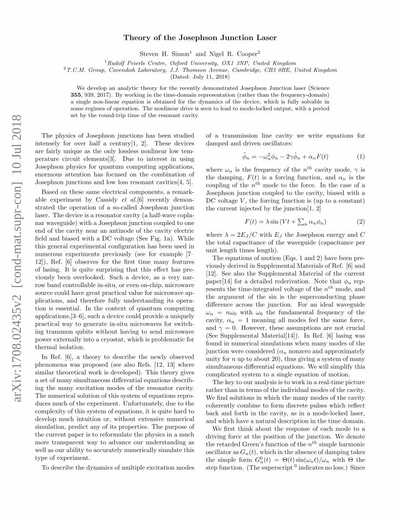
Based on these same electrical components, a remark-able experiment by Cassidy et al.[6] recently demon-strated the operation of a so-called Josephson junctionlaser. The device is a resonator cavity (a half-wave copla-nar waveguide) with a Josephson junction coupled to oneend of the cavity near an antinode of the cavity electricfield and biased with a DC voltage (See Fig. 1a). Whilethis general experimental configuration has been used innumerous experiments previously (see for example [7–12]), Ref. [6] observes for the first time many featuresof lasing. It is quite surprising that this effect has pre-viously been overlooked. Such a device, as a very nar-row band controllable in-situ, or even on-chip, microwavesource could have great practical value for microwave ap-plications, and therefore fully understanding its opera-tion is essential. In the context of quantum computingapplications,[3–6], such a device could provide a uniquelypractical way to generate in-situ microwaves for switch-ing transmon qubits without having to send microwavepower externally into a cryostat, which is problematic forthermal isolation.

In Ref. [6], a theory to describe the newly observedphenomena was proposed (see also Refs. [12, 13] wheresimilar theoretical work is developed). This theory givesa set of many simultaneous differential equations describ-ing the many excitation modes of the resonator cavity.The numerical solution of this system of equations repro-duces much of the experiment. Unfortunately, due to thecomplexity of this system of equations, it is quite hard todevelop much intuition or, without extensive numericalsimulation, predict any of its properties. The purpose ofthe current paper is to reformulate the physics in a muchmore transparent way to advance our understanding aswell as our ability to accurately numerically simulate thistype of experiment.

To describe the dynamics of multiple excitation modes

of a transmission line cavity we write equations fordamped and driven oscillators:

φn = −ω2nφn − 2γφn + αnF (t) (1)

where ωn is the frequency of the nth cavity mode, γ isthe damping, F (t) is a forcing function, and αn is thecoupling of the nth mode to the force. In the case of aJosephson junction coupled to the cavity, biased with aDC voltage V , the forcing function is (up to a constant)the current injected by the junction[1, 2]

F (t) = λ sin (V t+∑n αnφn) (2)

where λ = 2EJ/C with EJ the Josephson energy and Cthe total capacitance of the waveguide (capacitance perunit length times length).

The equations of motion (Eqs. 1 and 2) have been pre-viously derived in Supplemental Materials of Ref. [6] and[12]. See also the Supplemental Material of the currentpaper[14] for a detailed rederivation. Note that φn rep-resents the time-integrated voltage of the nth mode, andthe argument of the sin is the superconducting phasedifference across the junction. For an ideal waveguideωn = nω0 with ω0 the fundamental frequency of thecavity, αn = 1 meaning all modes feel the same force,and γ = 0. However, these assumptions are not crucial(See Supplemental Material[14]). In Ref. [6] lasing wasfound in numerical simulations when many modes of thejunction were considered (αn nonzero and approximatelyunity for n up to about 20), thus giving a system of manysimultaneous differential equations. We will simplify thiscomplicated system to a single equation of motion.

The key to our analysis is to work in a real-time picturerather than in terms of the individual modes of the cavity.We find solutions in which the many modes of the cavitycoherently combine to form discrete pulses which reflectback and forth in the cavity, as in a mode-locked laser,and which have a natural description in the time domain.

We first think about the response of each mode to adriving force at the position of the junction. We denotethe retarded Green’s function of the nth simple harmonicoscillator asGn(t), which in the absence of damping takesthe simple form G0

n(t) = Θ(t) sin(ωnt)/ωn with Θ thestep function. (The superscript 0 indicates no loss.) Since

arX

iv:1

708.

0243

5v2

[co

nd-m

at.s

upr-

con]

10

Jul 2

018

2

all of the modes couple to the same source, we group themall together by defining

Ψ =∑n αnφn . (3)

The voltage across the junction is simply VJ = V + Ψ.The retarded Green’s function for Ψ is then just K(t) =∑n α

2nGn(t). The dynamics of the system may then be

recast as a single equation

Ψ(t) = λ

∫ t

−∞dt′K(t− t′) sin[V t′ + Ψ(t′)] (4)

This is a highly nonlinear equation. As is often the casewith such equations, many solutions may exist and solu-tions may depend on initial conditions as well.

To understand the form of the kernel K(t), considerfirst the ideal case of no damping γ = 0 with ωn = nω0

and αn = 1. Then K has a sawtooth form K0(t) =(1/2)[T/2− (t mod T )] where T = 2π/ω0 is the “round-trip” time of the cavity. Once one adds damping, withγ ω0, to a very good approximation the response is thedecaying sawtooth (See also Supplemental Material[14])

K(t) = e−γtK0(t). (5)

It is important to note that even if one adds random-ness to the frequencies ωn and to the couplings αn thegeneral sawtooth form persists (See also SupplementalMaterial[14]). The sudden step reflects the fixed timedelay associated with the round-trip time of the cavity.

Note that in the case where Ψ 1, which results fromeither small λT 2 or large γT , we can treat Eq. 4 perturba-tively. At zeroth order, we drop Ψ on the right hand sideand have a simple integral on the right. For example, inthe case of large γT , one obtains Ψ(0)(t) = (λT/4γ) sinV twith the superscript here meaning at zeroth order. Wecan then plug this Ψ(0) into the right hand side of Eq. 4and again perform the integral, to obtain an improvedapproximation Ψ(1) at first order, and so forth. It iseasy to establish that this procedure only ever generatesharmonics of the frequency V , i.e., the time period ofoscillation is 2π/V . At large γT , this arises because thefunction K(t) has decayed to almost zero before reachingT , so its sawtooth form has been lost and the time periodT forgotten.

However, for small γT (believed to be appropriate forthe experiment[6]) with large λT 2 there is a different typeof solution where the oscillation period will instead be T .Most of the remainder of this paper will explore this case.

Using the form of Eqs. 5, we can transform Eq. 4 to

Ψ(t) = Ψ(t− T )e−γT + λ

∫ t

t−Tdt′K(t− t′) sin[V t′ + Ψ(t′)]

(6)The first term on the right represents the integration from−∞ to t−T . The interpretation is that a signal Ψ(t−T )

EJ

(a)

(b)

V

FIG. 1. (a) Circuit diagram for the Josephson junction laser(From Refs [6, 12, 13]). The cavity can be thought of asan LC chain (See Supplemental Material[14]). (b) Numericalform of Ψ(t) obtained by integration of Eq. 6 for parametersV = 2, γ = .01, λ = 6 in units where T = 2π so ω0 = 1. Thewaveform has constant negative slope with discrete steps of2π. Note that the two steps within each cycle are not equallyspaced but the pattern is periodic with period T .

has gone down the waveguide and returned after time Thaving decayed by e−γT . The resulting signal Ψ(t) is thisdecayed signal plus the result of driving by the Josephsonjunction during the period t− T to t.

Let us consider first the special case of γ = 0 and avoltage V that is commensurate with the period T . I.e.,we set V = Vm = 2πm/T for some integer m. Lookingfor a periodic solution we set Ψ(t−T ) = Ψ(t). Eq. 6 canthen be satisfied by having the sin be a constant sincethe integral of K0 over a period vanishes. Thus we set

Ψ(t) mod 2π = −Vmt+ β (7)

for some constant β. The right hand side is a linearlydecreasing function of time, but can be made periodic byinserting m phase slips of 2π during the cycle (i.e., mak-ing it a sawtooth). The phase slips may be at any pointin the cycle of time T , although they need to be the samefrom one cycle to the next to ensure T -periodicity. Thisanalytic solution matches numerical solutions for small γand commensurate V quite well as shown, for example, inFig. 1b. This form of solution remains valid for any formof K0(t) so long as its integral over a period vanishes.In particular this will be true for any parameters αn wechoose in Eq. 3 (See also Supplemental Material[14]). Weemphasize that this is the first completely analytic un-derstanding of this experimental system.

The power absorbed by the waveguide is P = (VJ −V )I = ΨEJ sin(V t+ Ψ). Here VJ −V = Ψ is the voltagefrom the injection point of the waveguide (the connec-tion of the Josephson junction to the waveguide) to theground. Thus the energy absorbed by the waveguide percycle is Eabsorbed =

∫ tt−T dt

′EJΨ(t′) sin(V t′ + Ψ(t′)) =−V TEJ〈sinβ〉 where we have integrated by parts (anddisregarded boundary terms assuming a periodic or al-

3

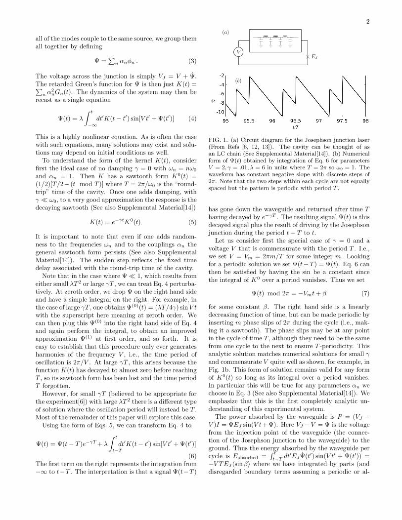
FIG. 2. Numerical form of Ψ(t) obtained by integration ofEq. 6 for parameters V = 4.02, γ = .05, λ = 12 in units whereT = 2π. (a) Oscillations of Ψ over several hundred periods.(b) Plot of 〈Ψ〉 which is Ψ averaged over a period T withvertical scale on the left, and also a plot of 〈sinβ〉 which issin[V t + Ψ] averaged over a period T with vertical scale onthe right. The two vertical scales are in ratio of λT 2/24 aspredicted by Eq. 9. The two curves (〈sinβ〉 and 〈Ψ〉) overlayso precisely that they are not both visible on this figure. Thediagonal dashed line is the predicted slope −δV t as discussedin the text. Note that when sinβ reaches −1 (the horizontaldashed line) the form of solution changes for a short periodof time.

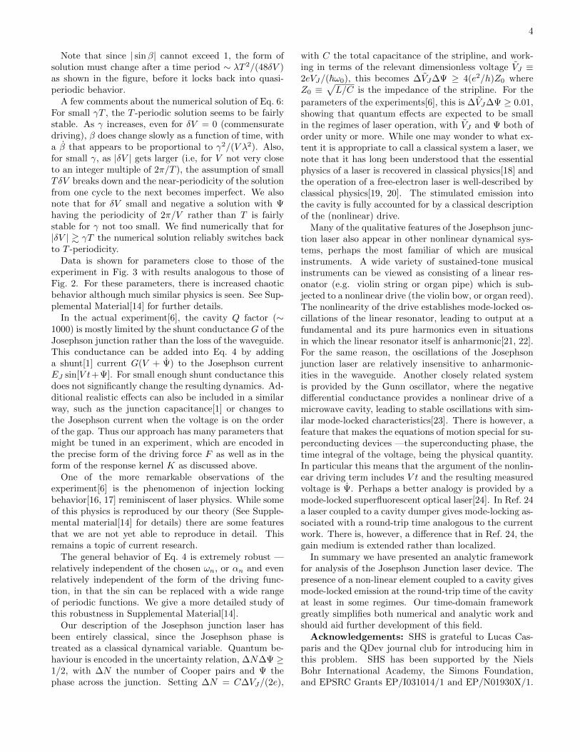
FIG. 3. As in Fig. 2 but for parameters closer to those of theexperiment: λ = 3, γ = .0005 and voltage V = 12.01. Againthe plots of 〈Ψ〉 and 〈sinβ〉 overlap so one cannot distinguishthe two curves. More examples and details are given in theSupplemental Material[14].

most periodic solution), and the brackets indicate theaverage of the sin over the cycle.

If there is a damping γ > 0 then there will be a lossper cycle of Estored(1−e−2γT ) where Estored is the storedenergy in the waveguide. For a steady state, we thusrequire that Estored = −V EJ〈sinβ〉/(2γ), for small γT .From this we can estimate the maximum waveguide volt-age (maximum Ψ).

Since Ψ is basically a sum of sawtooth waves, weconsider a sawtooth with a single 2π step which hasFourier modes sin(2πnt/T ) of amplitude 2/n. To de-termine the energy stored in each of these modes, re-fer back to Eq. 1 and note that the energy stored ina single oscillator is[15] Estored = C

4 V2max = C

4 (φn)2 =

C4

(2πnT

2n

)2= 4π2C

T 2 . To represent the finite slope of thesteps, we cut off the higher Fourier modes by using in-stead Fourier modes of amplitude (2/n)fn where fn isa some cutoff function which is unity at small n anddecays for large n. The total energy stored is thenEstored = (4π2C/T 2)

∑n f

2n whereas the maximum value

of the voltage will be Vmax = Ψmax = (4π/T )∑n fn.

Given that there are m = V T/(2π) phase slips per cyclewe add together all the energy in all of these pulses to getEstored = ξCV Vmax/2 where ξ =

∑f2n/

∑n fn. For fn

chosen as a sharp cutoff, ξ = 1 whereas for an exponen-tial cutoff fn = e−an instead we obtain ξ = 1/2. Settingthe energy stored to −V EJ〈sinβ〉/(2γ) with λ = 2EJ/Cwe obtain the result |Ψmax| = |Vmax| = λ

2ξγ |〈sinβ〉| withξ the unknown constant of order unity. Numerically wefind that this formula holds with 1/2 . ξ < 1 wheneverthe solution has near to T -periodicity.

With this maximum value of Ψ the sharp steps of Ψoccur over a time-scale δt ≈ 2π(2ξγ)/(λ|〈sinβ〉|). Dur-ing this time the argument of the sin wraps by 2π andsin[V t + Ψ] goes smoothly from 〈sinβ〉 to −1 to +1and then back to 〈sinβ〉. The total area under thisspike should then be roughly −2〈sinβ〉δt ≈ 4πγ/λ. (If〈sinβ〉 = −1 then it has to go all the way from −1 to 1giving a height of 2 whereas if 〈sinβ〉 = 0 then the spikegoes symmetrically up to 1 and down to −1 having netzero area.) Thus we can approximate

sin[V t+ Ψ(t)] = 〈sinβ〉+∑j(4πγ/λ)δ(t− tj) (8)

where tj are the particular times when the sawtooth stepsoccur. This can then be plugged into Eq. 4 and inte-grated. The second term is responsible for producing thesawtooth steps in Ψ since it is being integrated with thesawtooth function K. Note that the coefficient of thedelta function in Eq. 8 is exactly right to produce stepsof size 2π in Ψ. On the other hand, when we integrateEq. 8 in Eq. 4, using

∫ t−∞ dt′K(t− t′) = T 2/24, the first

term gives the relationship

〈Ψ〉 = λT 2〈sinβ〉/24 (9)

where again the brackets mean an average over a fullcycle. This relationship is very accurately confirmed nu-merically, not only for the case of commensurate voltagethat we have focussed on so far, but also more generally,as shown in Figs. 2b and 3b.

We can now consider the case where V deviates frombeing commensurate with the period T . We write V =Vm + δV where TδV 2π. We propose a solution ofthe form of Eq. 7 with Vm still commensurate and nowβ = −δV t is a slow function of time. We again assumethere are m phase slips of 2π per period and that theywill occur at the same points in each cycle. However nowΨ is no longer periodic in T but rather shifts by −δV Teach cycle as seen in Figs. 2 and 3. The frequency ofoscillation, however, remains ω0 = 2π/T very accurately.

4

Note that since | sinβ| cannot exceed 1, the form ofsolution must change after a time period ∼ λT 2/(48δV )as shown in the figure, before it locks back into quasi-periodic behavior.

A few comments about the numerical solution of Eq. 6:For small γT , the T -periodic solution seems to be fairlystable. As γ increases, even for δV = 0 (commensuratedriving), β does change slowly as a function of time, witha β that appears to be proportional to γ2/(V λ2). Also,for small γ, as |δV | gets larger (i.e, for V not very closeto an integer multiple of 2π/T ), the assumption of smallTδV breaks down and the near-periodicity of the solutionfrom one cycle to the next becomes imperfect. We alsonote that for δV small and negative a solution with Ψhaving the periodicity of 2π/V rather than T is fairlystable for γ not too small. We find numerically that for|δV | & γT the numerical solution reliably switches backto T -periodicity.

Data is shown for parameters close to those of theexperiment in Fig. 3 with results analogous to those ofFig. 2. For these parameters, there is increased chaoticbehavior although much similar physics is seen. See Sup-plemental Material[14] for further details.

In the actual experiment[6], the cavity Q factor (∼1000) is mostly limited by the shunt conductance G of theJosephson junction rather than the loss of the waveguide.This conductance can be added into Eq. 4 by addinga shunt[1] current G(V + Ψ) to the Josephson currentEJ sin[V t+Ψ]. For small enough shunt conductance thisdoes not significantly change the resulting dynamics. Ad-ditional realistic effects can also be included in a similarway, such as the junction capacitance[1] or changes tothe Josephson current when the voltage is on the orderof the gap. Thus our approach has many parameters thatmight be tuned in an experiment, which are encoded inthe precise form of the driving force F as well as in theform of the response kernel K as discussed above.

One of the more remarkable observations of theexperiment[6] is the phenomenon of injection lockingbehavior[16, 17] reminiscent of laser physics. While someof this physics is reproduced by our theory (See Supple-mental material[14] for details) there are some featuresthat we are not yet able to reproduce in detail. Thisremains a topic of current research.

The general behavior of Eq. 4 is extremely robust —relatively independent of the chosen ωn, or αn and evenrelatively independent of the form of the driving func-tion, in that the sin can be replaced with a wide rangeof periodic functions. We give a more detailed study ofthis robustness in Supplemental Material[14].

Our description of the Josephson junction laser hasbeen entirely classical, since the Josephson phase istreated as a classical dynamical variable. Quantum be-haviour is encoded in the uncertainty relation, ∆N∆Ψ ≥1/2, with ∆N the number of Cooper pairs and Ψ thephase across the junction. Setting ∆N = C∆VJ/(2e),

with C the total capacitance of the stripline, and work-ing in terms of the relevant dimensionless voltage VJ ≡2eVJ/(~ω0), this becomes ∆VJ∆Ψ ≥ 4(e2/h)Z0 whereZ0 ≡

√L/C is the impedance of the stripline. For the

parameters of the experiments[6], this is ∆VJ∆Ψ ≥ 0.01,showing that quantum effects are expected to be smallin the regimes of laser operation, with VJ and Ψ both oforder unity or more. While one may wonder to what ex-tent it is appropriate to call a classical system a laser, wenote that it has long been understood that the essentialphysics of a laser is recovered in classical physics[18] andthe operation of a free-electron laser is well-described byclassical physics[19, 20]. The stimulated emission intothe cavity is fully accounted for by a classical descriptionof the (nonlinear) drive.

Many of the qualitative features of the Josephson junc-tion laser also appear in other nonlinear dynamical sys-tems, perhaps the most familiar of which are musicalinstruments. A wide variety of sustained-tone musicalinstruments can be viewed as consisting of a linear res-onator (e.g. violin string or organ pipe) which is sub-jected to a nonlinear drive (the violin bow, or organ reed).The nonlinearity of the drive establishes mode-locked os-cillations of the linear resonator, leading to output at afundamental and its pure harmonics even in situationsin which the linear resonator itself is anharmonic[21, 22].For the same reason, the oscillations of the Josephsonjunction laser are relatively insensitive to anharmonic-ities in the waveguide. Another closely related systemis provided by the Gunn oscillator, where the negativedifferential conductance provides a nonlinear drive of amicrowave cavity, leading to stable oscillations with sim-ilar mode-locked characteristics[23]. There is however, afeature that makes the equations of motion special for su-perconducting devices —the superconducting phase, thetime integral of the voltage, being the physical quantity.In particular this means that the argument of the nonlin-ear driving term includes V t and the resulting measuredvoltage is Ψ. Perhaps a better analogy is provided by amode-locked superfluorescent optical laser[24]. In Ref. 24a laser coupled to a cavity dumper gives mode-locking as-sociated with a round-trip time analogous to the currentwork. There is, however, a difference that in Ref. 24, thegain medium is extended rather than localized.

In summary we have presented an analytic frameworkfor analysis of the Josephson Junction laser device. Thepresence of a non-linear element coupled to a cavity givesmode-locked emission at the round-trip time of the cavityat least in some regimes. Our time-domain frameworkgreatly simplifies both numerical and analytic work andshould aid further development of this field.Acknowledgements: SHS is grateful to Lucas Cas-

paris and the QDev journal club for introducing him inthis problem. SHS has been supported by the NielsBohr International Academy, the Simons Foundation,and EPSRC Grants EP/I031014/1 and EP/N01930X/1.

5

NRC is supported by EPSRC Grants EP/P034616/1 andEP/K030094/1.

[1] A. Barone and G. Paterno, Physics and Applications ofthe Josephson Effect (Wiley-VCH Verlag GmbH & Co.KGaA, 1982).

[2] K. K. Likharev, The Dynamics of Josephson Junctionsand Circuits (Gordon and Breach, New York, 1984).

[3] M. H. Devoret, A. Wallraff, and J. M. Martinis, (2004),arXiv:cond-mat/0411174.

[4] M. H. Devoret and R. J. Schoelkopf, Science 339, 1169(2013).

[5] Quantum machines : measurement and control of engi-neered quantum systems, Ecole d’ete physique theorique(Les Houches, Haute-Savoie, France), Vol. 96 (OxfordUniversity Press, 2014).

[6] M. C. Cassidy, A. Bruno, S. Rubbert, M. Irfan,J. Kammhuber, R. N. Schouten, A. R. Akhmerov,and L. P. Kouwenhoven, Science 355, 939 (2017),http://science.sciencemag.org/content/355/6328/939.full.pdf.

[7] M. Hofheinz, F. Portier, Q. Baudouin, P. Joyez, D. Vion,P. Bertet, P. Roche, and D. Esteve, Phys. Rev. Lett.106, 217005 (2011).

[8] C. M. Wilson, G. Johansson, A. Pourkabirian,M. Simoen, J. R. Johansson, T. Duty, F. Nori, andP. Delsing, Nature 479, 376 (2011).

[9] F. Chen, A. J. Sirois, R. W. Simmonds, and A. J.Rimberg, Applied Physics Letters 98, 132509 (2011),http://dx.doi.org/10.1063/1.3573824.

[10] F. Chen, J. Li, A. D. Armour, E. Brahimi, J. Stetten-heim, A. J. Sirois, R. W. Simmonds, M. P. Blencowe,and A. J. Rimberg, Phys. Rev. B 90, 020506 (2014).

[11] V. Gramich, B. Kubala, S. Rohrer, and J. Ankerhold,Phys. Rev. Lett. 111, 247002 (2013).

[12] A. D. Armour, M. P. Blencowe, E. Brahimi, and A. J.Rimberg, Phys. Rev. Lett. 111, 247001 (2013).

[13] S. Meister, M. Mecklenburg, V. Gramich, J. T. Stock-burger, J. Ankerhold, and B. Kubala, Phys. Rev. B 92,174532 (2015).

[14] S. H. Simon and N. R. Cooper, Supplemental Material(2017).

[15] Because the spatial form of the voltage is Vn(x) =Vn cos(2πnx/`), the total energy stored is half of theusual CV 2/2. See Supplemental Material[14].

[16] R. Adler, Proceedings of the IRE 34, 351 (1946).[17] Y.-Y. Liu, J. Stehlik, M. J. Gullans, J. M. Taylor, and

J. R. Petta, Phys. Rev. A 92, 053802 (2015).[18] M. Borenstein and W. E. Lamb, Phys. Rev. A 5, 1298

(1972).[19] F. Hopf, P. Meystre, M. Scully, and W. Louisell, Optics

Communications 18, 413 (1976).[20] E. Saldin, E. Schneidmiller, and M. Yurkov, The Physics

of Free Electron Lasers (Springer, 2000).[21] N. H. Fletcher, Reports on Progress in Physics 62, 723

(1999).[22] A. Jenkins, Physics Reports 525, 167 (2013), self-

oscillation.[23] W.-C. Tsai, F. J. Rosenbaum, and L. A. MacKenzie,

IEEE Transactions on Microwave Theory and Techniques18, 808 (1970).

[24] J. D. Harvey, R. Leonhardt, P. D. Drummond, andS. Carter, Phys. Rev. A 40, 4789 (1989).

1

Supplemental Materials: Theory of the Josephson Junction Laser

Supp. 1: Derivation of Eq. 1

Although Eq. 1 was given in Ref. [6] (see also Ref. [12])and also for a single mode in [13] we give a re-derivationof it here for completeness. For simplicity we will performthe derivation in the absence of loss. The inclusion of lossis quite straightforward.

We begin with the telegrapher’s equation for a waveg-uide. Treating the system as a string of coupled inductorsand capacitors we have the consitituitive equations

∂xI = −C∂tV (S1)

∂xV = −L∂tI (S2)

where V is the electostatic potential, and I is the current.Here C is the capacitance per unit length and L is theinductance per unit length. One can view the system asbeing made of discrete elements separated by distance a,with La and Ca the inductance and capacitance of eachindividual element.

The boundary conditions for a half-wave cavity oflength ` are I(x = 0) = I(x = `) = 0 and correspondingly∂xV(x = 0) = ∂xV(x = `) = 0. Given these boundaryconditions, we can write

I =∑n>0

In(t) sin(2πnx/`) (S3)

V =∑n≥0

Vn(t) cos(2πnx/`) (S4)

We now couple in the Josephson junction at positionxi. This injects current Iin = Ej sin(ϕ) at position xiwhere ϕ is the phase across the junction (which we willdetermine later) and we have set 2e/~ = 1 as before. Dueto this current injection, we modify Eq. S1 to read

∂xI = −C∂tV + Iin(ϕ)δ(x− xi) (S5)

We can then decompose Eqns. S5 and S2 into spatialFourier modes giving (for m > 0)

(2πm)Im = −C ∂tVm + 2 cos(2πmxi/`)Iin(ϕ) (S6)

(2πm)Vm = L∂tIm (S7)

where C = C` is the total capacitance and L = L` thetotal inductance. Defining

φm =

∫ t

−∞Vm(t′)dt′

we have Eq. S7 written as

Im = 2πmφm/L

which we plug into Eq. S6 to obtain

(2πm)2

Lφm = −C∂2t φm + 2αmIin(ϕ) (S8)

where we have defined

αm = cos(2πmxi/`). (S9)

In the experiment, the injection point xi is very close tothe end of the cavity so αm ≈ 1 for m not too large.However, there is no reason not to consider the moregeneral case.

Looking also at the voltage at the injection point wehave

V(xin) =∑m≥0

αmVm

The waveguide is DC-biased using the techinque ofRef. [9], which couples to the V0 mode which we thenidentify as the applied voltage V . We thus have

ϕ(t) =

∫ t

−∞dt′V(xin, t

′) = V t+∑m>0

αmφm(t)

Plugging this into Eq. S8 obtains our final result Eq. 1,except for the loss term which we have dropped only forconvenience of notation here.

Supp. 2: The Green’s Function

Given a damped harmonic oscillator with a δ functionsource

φ = −ω2φ− 2γφ+ δ(t), (S10)

it is easy to show that the response is

G(t) =e−γt sin ωt

ωΘ(t)

where

ω =√ω2 − γ2.

Now defining

Ψ =∑n

αnφn

we get a response function for Ψ given by

K(t) =∑n

α2n

e−γt sin ωnt

ωnΘ(t). (S11)

2

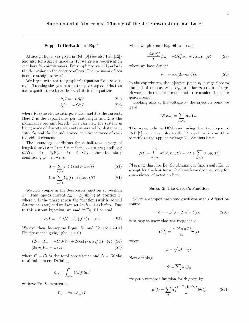
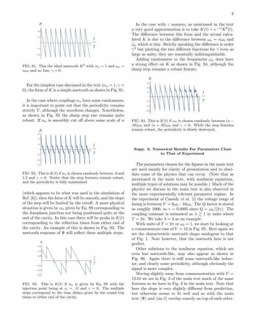
FIG. S1. This the ideal sawtooth K0 with αn = 1 and ωn =nω0 and no loss, γ = 0.

For the simplest case discussed in the text (αn = 1, γ =0), the form ofK is a simple sawtooth as shown in Fig. S1.

In the case where couplings αn have some randomness,it is important to point out that the periodicity remainsstrictly T , although the waveform changes. Nonetheless,as shown in Fig. S2 the sharp step rise remains quiterobust. If αn is smoothly cut off above some scale of n

FIG. S2. This is K(t) if αn is chosen randomly between .8 and1.2 and γ = 0. Notice that the step features remain robust,and the periodicity is fully maintained.

(which appears to be what was used in the simulation ofRef. [6]), then the form ofK will be smooth, and the slopeof the step will be limited by the cutoff. A more physicalsituation is given by αn given by Eq. S9 corresponding tothe Josephson junction not being positioned quite at theend of the cavity. In this case there will be peaks in K(t)corresponding to the reflection times from either end ofthe cavity. An example of this is shown in Fig. S3. Thesawtooth response of Ψ will reflect these multiple steps.

FIG. S3. This is K(t) if αn is given by Eq. S9 with theinjection point being at xi = .1` and γ = 0. The multiplesteps correspond to the time delays given by the round triptimes to either end of the cavity.

In the case with γ nonzero, as mentioned in the texta very good approximation is to take K(t) = e−γtK0(t).The difference between this form and the actual calcu-lated K is due to the difference between ωn = nω0 andωn which is tiny. Strictly speaking the difference is orderγ2 but plotting the two different functions for γ even aslarge as unity, they are essentially indistinguishable.

Adding randomness to the frequencies ωn does havea strong effect on K as shown in Fig. S4, although thesharp step remains a robust feature.

FIG. S4. This is K(t) if ωn is chosen randomly between (n−.05)ω0 and (n + .05)ω0 and γ = 0. While the step featuresremain robust, the periodicity is slowly destroyed.

Supp. 3: Numerical Results For Parameters Closeto That of Experiment

The parameters chosen for the figures in the main textare used mainly for clarity of presentation and to eluci-date some of the physics that can occur. (Note that asmentioned in the main text, with nonlinear equations,multiple types of solutions may be possble.) Much of thephysics we discuss in the main text is also observed inthe more experimentally relevant parameter regime. Inthe experiment of Cassidy et al. [1] the voltage range oflasing is between V = 6ω0−16ω0. The Q-factor is statedas roughly 1000, so γ = 0.0005 since Q = ω0/(2γ). Thecoupling constant is estimated as λ & 1 in units whereT = 2π. We take λ = 3 as an example.

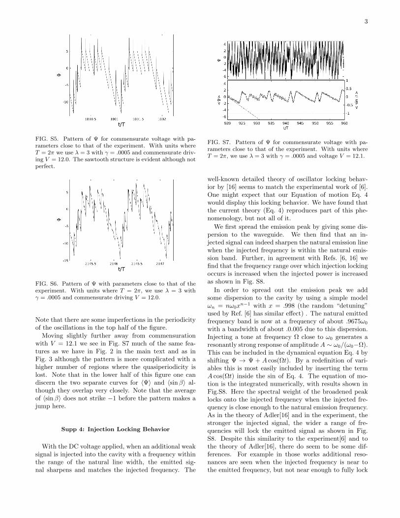
With units of T = 2π or ω0 = 1, we start by looking ata commensurate case of V = 12 in Fig. S5. Here again wesee the characteristic sawtooth shape analogous to thatof Fig. 1. Note however, that the sawtooth here is notperfect.

Other solutions to the nonlinear equation, which areeven less sawtooth-like, may also appear as shown inFig. S6. Again there is still some sawtooth-like behav-ior, and clearly some periodicity, although obviously thesignal is more complex.

Moving slightly away from commensuration with V =12.01 we see in Fig. 3 of the main text much of the samefeatures as we have in Fig. 2 in the main text. Note thathere the slope is very slightly different from prediction,but otherwise seems to fit well and as with the maintext 〈Ψ〉 and 〈sinβ〉 overlay exactly on top of each other.

3

FIG. S5. Pattern of Ψ for commensurate voltage with pa-rameters close to that of the experiment. With units whereT = 2π we use λ = 3 with γ = .0005 and commensurate driv-ing V = 12.0. The sawtooth structure is evident although notperfect.

FIG. S6. Pattern of Ψ with parameters close to that of theexperiment. With units where T = 2π, we use λ = 3 withγ = .0005 and commensurate driving V = 12.0.

Note that there are some imperfections in the periodicityof the oscillations in the top half of the figure.

Moving slightly further away from commensurationwith V = 12.1 we see in Fig. S7 much of the same fea-tures as we have in Fig. 2 in the main text and as inFig. 3 although the pattern is more complicated with ahigher number of regions where the quasiperiodicity islost. Note that in the lower half of this figure one candiscern the two separate curves for 〈Ψ〉 and 〈sinβ〉 al-though they overlap very closely. Note that the averageof 〈sinβ〉 does not strike −1 before the pattern makes ajump here.

Supp 4: Injection Locking Behavior

With the DC voltage applied, when an additional weaksignal is injected into the cavity with a frequency withinthe range of the natural line width, the emitted sig-nal sharpens and matches the injected frequency. The

FIG. S7. Pattern of Ψ for commensurate voltage with pa-rameters close to that of the experiment. With units whereT = 2π, we use λ = 3 with γ = .0005 and voltage V = 12.1.

well-known detailed theory of oscillator locking behav-ior by [16] seems to match the experimental work of [6].One might expect that our Equation of motion Eq. 4would display this locking behavior. We have found thatthe current theory (Eq. 4) reproduces part of this phe-nomenology, but not all of it.

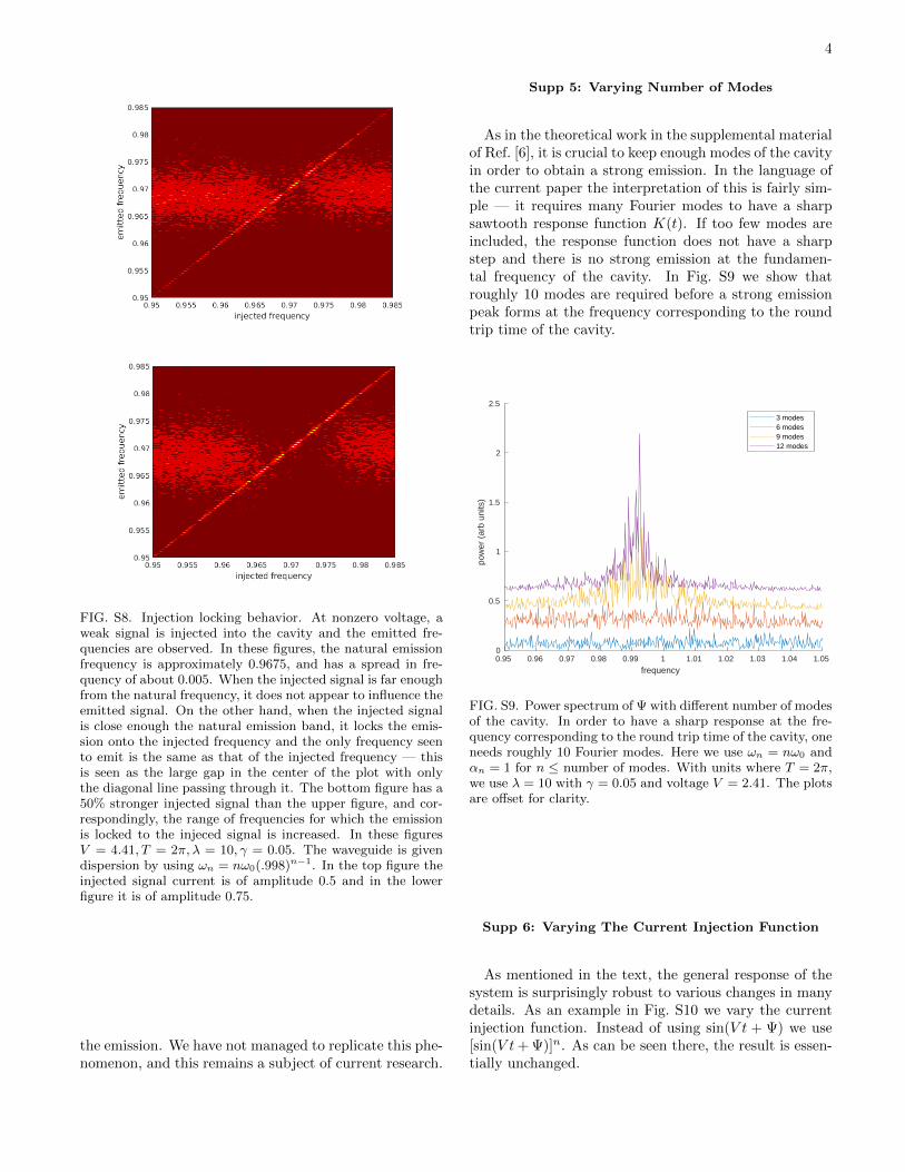
We first spread the emission peak by giving some dis-persion to the waveguide. We then find that an in-jected signal can indeed sharpen the natural emission linewhen the injected frequency is within the natural emis-sion band. Further, in agreement with Refs. [6, 16] wefind that the frequency range over which injection lockingoccurs is increased when the injected power is increasedas shown in Fig. S8.

In order to spread out the emission peak we addsome dispersion to the cavity by using a simple modelωn = nω0x

n−1 with x = .998 (the random “detuning”used by Ref. [6] has similar effect) . The natural emittedfrequency band is now at a frequency of about .9675ω0

with a bandwidth of about .0.005 due to this dispersion.Injecting a tone at frequency Ω close to ω0 generates aresonantly strong response of amplitude A ∼ ω0/(ω0−Ω).This can be included in the dynamical equation Eq. 4 byshifting Ψ → Ψ + A cos(Ωt). By a redefinition of vari-ables this is most easily included by inserting the termA cos(Ωt) inside the sin of Eq. 4. The equation of mo-tion is the integrated numerically, with results shown inFig.S8. Here the spectral weight of the broadened peaklocks onto the injected frequency when the injected fre-quency is close enough to the natural emission frequency.As in the theory of Adler[16] and in the experiment, thestronger the injected signal, the wider a range of fre-quencies will lock the emitted signal as shown in Fig.S8. Despite this similarity to the experiment[6] and tothe theory of Adler[16], there do seem to be some dif-ferences. For example in those works additional reso-nances are seen when the injected frequency is near tothe emitted frequency, but not near enough to fully lock

4

FIG. S8. Injection locking behavior. At nonzero voltage, aweak signal is injected into the cavity and the emitted fre-quencies are observed. In these figures, the natural emissionfrequency is approximately 0.9675, and has a spread in fre-quency of about 0.005. When the injected signal is far enoughfrom the natural frequency, it does not appear to influence theemitted signal. On the other hand, when the injected signalis close enough the natural emission band, it locks the emis-sion onto the injected frequency and the only frequency seento emit is the same as that of the injected frequency — thisis seen as the large gap in the center of the plot with onlythe diagonal line passing through it. The bottom figure has a50% stronger injected signal than the upper figure, and cor-respondingly, the range of frequencies for which the emissionis locked to the injeced signal is increased. In these figuresV = 4.41, T = 2π, λ = 10, γ = 0.05. The waveguide is givendispersion by using ωn = nω0(.998)n−1. In the top figure theinjected signal current is of amplitude 0.5 and in the lowerfigure it is of amplitude 0.75.

the emission. We have not managed to replicate this phe-nomenon, and this remains a subject of current research.

Supp 5: Varying Number of Modes

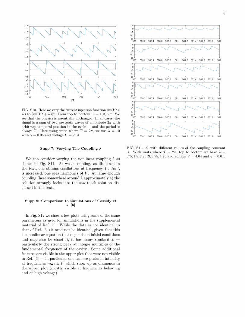
As in the theoretical work in the supplemental materialof Ref. [6], it is crucial to keep enough modes of the cavityin order to obtain a strong emission. In the language ofthe current paper the interpretation of this is fairly sim-ple — it requires many Fourier modes to have a sharpsawtooth response function K(t). If too few modes areincluded, the response function does not have a sharpstep and there is no strong emission at the fundamen-tal frequency of the cavity. In Fig. S9 we show thatroughly 10 modes are required before a strong emissionpeak forms at the frequency corresponding to the roundtrip time of the cavity.

0.95 0.96 0.97 0.98 0.99 1 1.01 1.02 1.03 1.04 1.05

frequency

0

0.5

1

1.5

2

2.5

pow

er (

arb

units

)

3 modes6 modes9 modes12 modes

FIG. S9. Power spectrum of Ψ with different number of modesof the cavity. In order to have a sharp response at the fre-quency corresponding to the round trip time of the cavity, oneneeds roughly 10 Fourier modes. Here we use ωn = nω0 andαn = 1 for n ≤ number of modes. With units where T = 2π,we use λ = 10 with γ = 0.05 and voltage V = 2.41. The plotsare offset for clarity.

Supp 6: Varying The Current Injection Function

As mentioned in the text, the general response of thesystem is surprisingly robust to various changes in manydetails. As an example in Fig. S10 we vary the currentinjection function. Instead of using sin(V t + Ψ) we use[sin(V t+ Ψ)]n. As can be seen there, the result is essen-tially unchanged.

5

-20

-15

-10

-15

-10

-5

-15

-10

-5

700 701 702 703 704 705

t/T

-14-12-10

-8-6-4

FIG. S10. Here we vary the current injection function sin(V t+Ψ) to [sin(V t+ Ψ)]n. From top to bottom, n = 1, 3, 5, 7. Wesee that the physics is essentially unchanged. In all cases, thesignal is a sum of two sawtooth waves of amplitude 2π witharbitrary temporal position in the cycle — and the period isalways T . Here using units where T = 2π, we use λ = 10with γ = 0.05 and voltage V = 2.04

Supp 7: Varying The Coupling λ

We can consider varying the nonlinear coupling λ asshown in Fig. S11. At weak coupling, as discussed inthe text, one obtains oscillations at frequency V . As λis increased, one sees harmonics of V . At large enoughcoupling (here somewhere around λ approximately 4) thesolution strongly locks into the saw-tooth solution dis-cussed in the text.

Supp 8: Comparison to simulations of Cassidy etal.[6]

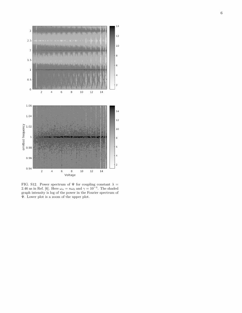
In Fig. S12 we show a few plots using some of the sameparameters as used for simulations in the supplementalmaterial of Ref. [6]. While the data is not identical tothat of Ref. [6] (it need not be identical, given that thisis a nonlinear equation that depends on initial conditionsand may also be chaotic), it has many similarities —particularly the strong peak at integer multiples of thefundamental frequency of the cavity. Some additionalfeatures are visible in the upper plot that were not visiblein Ref. [6] — in particular one can see peaks in intensityat frequencies mω0 ± V which show up as diamonds inthe upper plot (mostly visible at frequencies below ω0

and at high voltage).

500 500.2 500.4 500.6 500.8 501 501.2 501.4 501.6 501.8 502-15

-10

-5

0

5

500 500.2 500.4 500.6 500.8 501 501.2 501.4 501.6 501.8 502-15

-10

-5

0

5

500 500.2 500.4 500.6 500.8 501 501.2 501.4 501.6 501.8 502-15

-10

-5

0

5

500 500.2 500.4 500.6 500.8 501 501.2 501.4 501.6 501.8 502-15

-10

-5

0

5

500 500.2 500.4 500.6 500.8 501 501.2 501.4 501.6 501.8 502-15

-10

-5

0

5

500 500.2 500.4 500.6 500.8 501 501.2 501.4 501.6 501.8 502-15

-10

-5

0

5

FIG. S11. Ψ with different values of the coupling constantλ. With units where T = 2π, top to bottom we have λ =.75, 1.5, 2.25, 3, 3.75, 4.25 and voltage V = 4.04 and γ = 0.01.

6

FIG. S12. Power spectrum of Ψ for coupling constant λ =2.46 as in Ref. [6]. Here ωn = nω0 and γ = 10−4. The shadedgraph intensity is log of the power in the Fourier spectrum ofΨ. Lower plot is a zoom of the upper plot.