THEORETICAL PREDICTION OF COUNTER-ROTATING …

THEORETICAL PREDICTION OF COUNTER-ROTATING PROPELLER NOISE

by

ANTHONY BRIAN PARRY

Being an account of research carried out in the

Department of Applied Mathematical Studies, University

of Leeds, under the supervision of Professor D. G. Crighton

Submitted in accordance with the requirements

for the degree of Doctor of Philosophy

February, 1988

ABSTRACT

A theoretical prediction scheme has been developed for the tone

noise generated by a counter-rotation propeller.

We start by deriving formulae for the harmonic components of the

far acoustic field generated by the thickness and steady loading noise

sources. Excellent agreement is shown between theory and measurements.

Asymptotic approximation techniques are described which enable us to

simplify considerably the complex radiation formulae, whilst retaining

all of their important characteristics, and thus save, typically, 95%

of computer processing time.

Next we derive formulae for the radiated sound field generated by

aerodynamic interactions between the blade rows. Here, however, the inputs

to the formulae include a knowledge of the fluctuating blade pressure

fields which cannot generally be assumed given and must therefore be

calculated within the prediction scheme.

In the case of viscous wake interactions we consider various models

for the wake profile which is written as a series of harmonic gusts. The

fluctuating pressure distribution on the downstream blades can then be

calculated in the high frequency limit. Comparisons are made between

measurements and predictions for a counter-rotation propeller and for rotor/

stator interaction on a model fan rig.

For potential field interactions we describe the flow fields due to

blade circulation and blade thickness in terms of harmonic gusts with the

flow assumed incompressible. The blade response is calculated for both

finite and semi-infinite airfoils. Some important differences between these

two cases are noted in both high and low frequency limits. Predicted noise

levels are much improved over those obtained using only the viscous wake

model. The inclusion of compressibility, in both flow field and airfoil

response calculations, provides a further improvement in the predicted

noise levels. The discrepancy between measurements and predictions at

this stage is, typically, 2 or 3 dB.

ACKNOWLEDGEMENTS

First and foremost I would like to express sincere thanks to

Professor D. G. Crighton for his insuperable help, encouragement and

enthusiasm. During the three years it has taken to prepare this thesis,

I found our regular discussion sessions to be most stimulating; these

discussions managed to rekindle in me an appetite for applied mathematics

that I thought I had left behind in the sixth form. For this I shall

always be grateful.

I would like to thanks Rolls-Royce plc. for allowing me to pursue

my studies, and for releasing some experimental data.

In addition, my colleagues at Rolls-Royce plc. deserve a mention.

In particular, I am indebted to Dr. A. J. Kempton for many helpful

discussions, and to Dr. A. M. Cargill for a number of invaluable suggestions

relating to the work in chapters 5,6 and 7.

The financial support of the S. E. R. C., through the award of an

Industrial Studentship, and of Rolls-Royce plc., is also gratefully

acknowledged.

Finally, I must compliment Mrs. L. Trundle on her meticulous typing,

of both text and formulae, and Mr. C. J. Knighton on his handiwork in

preparing the figures.

TO

DEANA, JENNIFER AND KATE

CONTENTS

1. INTRODUCTION 1

2. SINGLE-ROTATION PROPELLER NOISE 6

2.1 Introduction 6

2.2 Steady Loading Noise 7

2.3 Thickness Noise 17

2.4 Comparison with Measurements 21

2.5 Nonlinear Effects 24

3. ASY: PTOTIC APPROXIMATIONS FOR ROTOR ALONE NOISE 27

3.1 Introduction 27

3.2 Subsonic Operating Conditions 28

3.2.1 A Straight Bladed Propeller 28

3.2.2 A Swept Propeller 37

3.3 Supersonic Operating Conditions 40

3.3.1 A Straight Bladed Propeller 40

3.3.2 Chordwise Noncompactness Effects 44

3.4 Uniform Asymptotic Approximations 50

3.4.1 Bessel Function Approximations 50

3.4.2 The Transonic Regime 56

3.4.3 The Supersonic Regime 64

APPENDICES 71

A3.1 Harmonic Series for Straight-Bladed, Chordwise 71

Compact, Supersonic Propellers

A3.2 Harmonic Series for Chordwise Noncompact, Supersonic 74

Propellers

A3.3 Asymptotic Overlap of Bessel Function Approximations 77

4. COUNTER-ROTATION PROPELLER NOISE 80

4.1 Introduction 80

4.2 Downstream Interactions 82

4.3 Upstream Interactions 86

4.4 Asymptotic Approximations 88

4.5 Discussion 90

5. WAKE INTERACTIONS 93

5.1 Introduction 93

5.2 Wake Models 94

5.2.1 Prandtl's Mixing Length Theory 94

5.2.2 Schlichting Wake Model 99

5.2.3 Gaussian Wake Model 102

5.2.4 'Experiments 103

5.3 Harmonic Gusts 106

5.3.1 Coordinate System for Wake 107

5.3.2 Schlichting Wake Model 109

5.3.3 Gaussian Wake Model 111

5.3.4 Reynolds Wake Model 112

5.4 Airfoil Response 112

5.4.1 Coordinate System for Downstream Blades 112

5.4.2 High Frequency Response 115

5.5 Measurement vs Prediction 117

5.5.1 Counter-Rotation Propeller 117

5.5.2 Rotor-Stator Interaction 121

APPENDICES - 126

A5.1 Fourier Coefficients for the Schlichting Wake Model 126

6. POTENTIAL FIELD INTERACTIONS - INCOMPRESSIBLE FLOW 128

6.1 Introduction 128

6.2 Potential Field due to Blade Thickness 130

6.2.1 Velocity Potential 130

6.2.2 Upwash on Upstream Airfoil 134

6.2.3 Upwash on Downstream Airfoil 137

6.3 Potential Field due to Blade Circulation 138

6.3.1 Stream Function 138


6.3.3 Uowash on Downstream Airfoil 141

6.4 Response of Upstream Airfoil (Semi-Infinite) 142

6.5 Response of Downstream Airfoil (Semi-Infinite) 145

6.6 Response of Finite Chord Airfoil 146

6.7 Finite Airfoil vs Semi-Infinite Airfoil 149

6.7.1 Pressure 149

6.7.2 Lift per unit Span 152

6.7.3 The Factor of n/4 154

6.8 Measurement vs Prediction 158.

APPENDICES 166

A6.1 The Potential Field of an Ellipse 166

A6.2 Chordwise Integration (Finite Airfoil) 169

A6.3 High Frequency Response of a Finite Airfoil 171

A6.4 Chordwise Integration (Finite Airfoil with c} co) 173

A6.5 Low Frequency Effects 176

1. Total Unsteady Lift 176

1.1 Finite Airfoil 176

1.2 Upstream Semi-Infinite Airfoil 177

1.3 Downstream Semi-Infinite Airfoil 178

2. Unsteady Pressure 178

2.1 Finite Airfoil 178

2.2 Upstream Semi-Infinite Airfoil 180

2.3 Downstream Semi-Infinite Airfoil 180

7. POTENTIAL FIELD INTERACTIONS - COMPRESSIBLE FLOW 181


7.2 Potential Field due to Blade Thickness 183




7.3 Potential Field due to Blade Circulation 190




7.4 Response of the Upstream Row 196

7.5 Leading Edge Correction 210

7.6 Response of the Downstream Row 217

7.7 Low Frequency Response 222

7.8 Measurement vs Prediction 227

APPENDICES 234

A7.1 Dirac Delta Functions 234

A7.2 Velocity Potential for a Point Vortex in Incompressible 236

Flow

A7.3 The Kutta Condition 238

A7.4 Chordwise Integration (Low Frequency) 240

8. FURTHER WORK 244


8.2 Approximations 244

8.3 Installation Effects 246

8.4 Extensions

8.5 Further Topics

247

249

REFERENCES 252

LIST OF FIGURES

Figure 2.1 The nominal propeller disc plane. 9

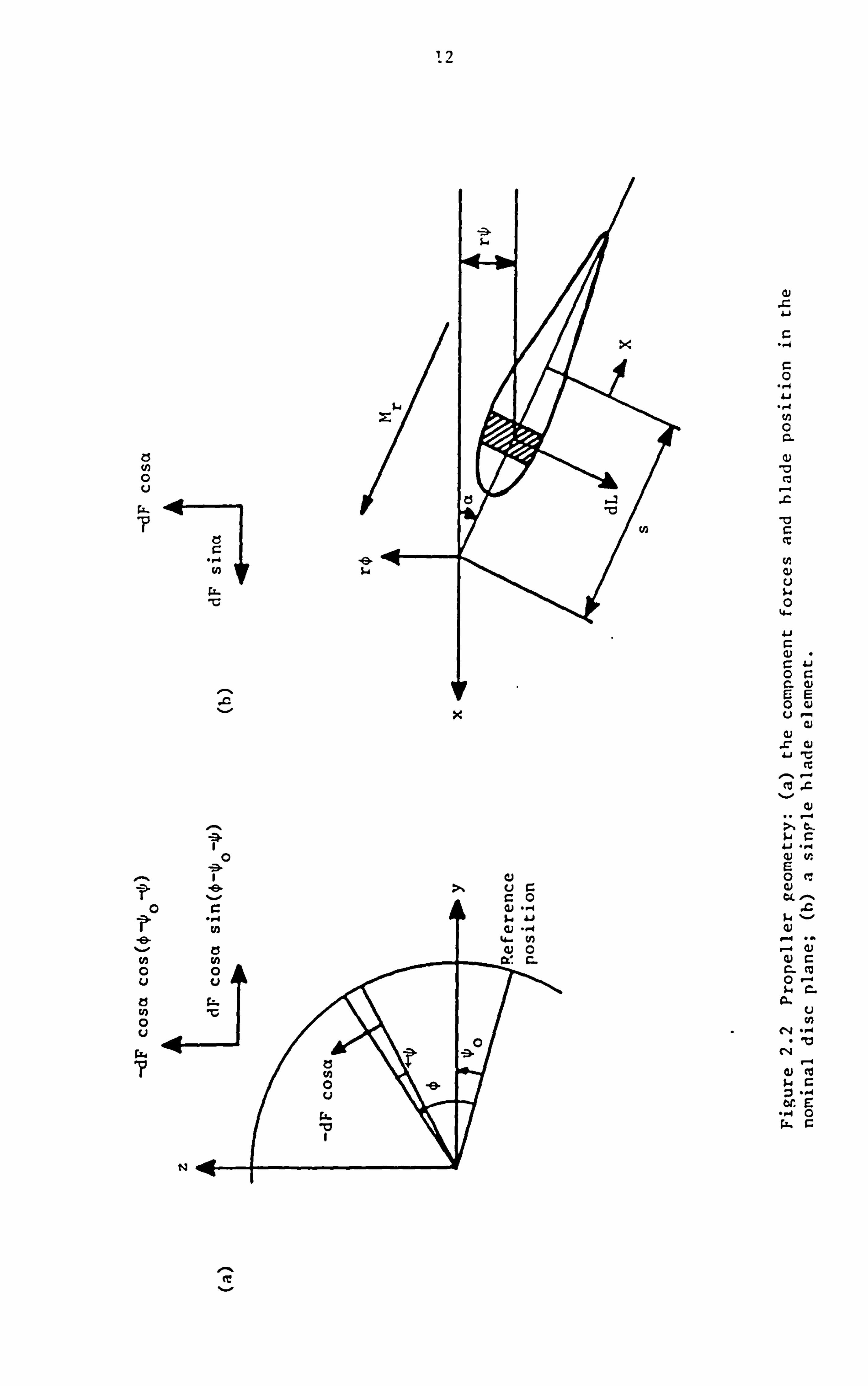
Figure 2.2 Propeller 12 geometry: (a) the component forces and blade position in the nominal disc plane; (b) a single blade element.

Figures 2.3,2.4 Gannet measurements vs predictions (first and 22 second harmonic).

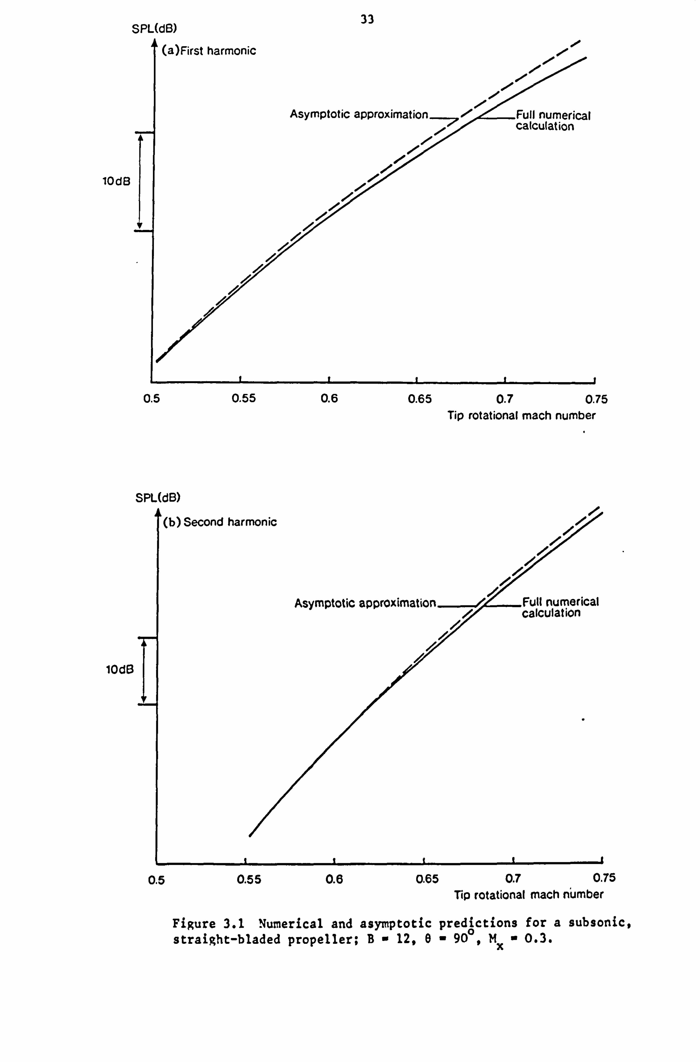
Figure 3.1 Numerical and asymptotic predictions for a subsonic, 33 = 0.3 straight-bladed propeller; B= 12,8 = 90°, M :

x (a) first harmonic; (b) second harmonic.

Figure 3.2 The relationship between 8t and Mobs' 35

Figure 3.3 Numerical and asymptotic predictions of the effect 35 = 500 of blade sweep on a subsonic propeller; A

t

Figure 3.4 Comparisons between numerical and asymptotic 43

predictions for a supersonic, straight-bladed propeller.

Figure 3.5 Numerical and asymptotic predictions of the effect 43

of chordwise noncompactness.

Figure 3.6 Asymptotic calculation of propeller noise vs tip 51

relative Mach number. ' For M <1 we use (3.2.9) rt

and for M >, l we use (3.3.5). rt

Figure 3.7 Comparisons between first and second order asymptotic 51 predictions and numerical calculations for a supersonic, straight-bladed propeller.

Figure 4.1 Front and rear blade row configurations (at constant 83 radius) on a counter-rotation propeller.

Table 5.1 Coefficients for the near wakes and far wakes from 105 isolated airfoils, cascades and rotor.

Figure 5.1 Coordinate system for downstream gust interaction. 108

Figures 5.2-5.4 Gannet measurements vs predictions for the (1,1), 108, (1,2) and (2,1) interaction tones. 119

Figures 5.5,5.6 Predicted wake interaction noise vs rotor-rotor 122

spacing for the (1,1) interaction tone on a7x7 propfan, and for blade passing frequency on a 27-bladed fan rig.

Table 5.2 Predicted PWL levels, relative to measureirents, for 123

the Rolls-Royce 27-bladed fan rig.

Figure 6.1 The cross section of each blade is represented by an 132

ellipse of ni. nor axis a and major axis h.

Figure 6.2 Coordinate systems for the interaction of the 132 rear row potential field with the front row blades.

Figure 6.3 The potential field due to blade circulation can 140 be modelled by replacing each blade section with a point vortex having the same circulation.

Figure 6.4 Contour used to evaluate the integral in (6.7.3). 140

Figures 6.5-6.10 Gannet measurements vs predictions for the (1,1), 160, (2,1) and (1,2) interaction tones. The potential 161, field predictions are obtained using both semi- 163 infinite and finite airfoil response calculations in incompressible flow.

Figure 6.11 Conformal mapping from a circle in the E-plane 167 to an ellipse in the z-plane.

Figure 7.1 Vortex positions in original and transformed 192

coordinate systems.

Figure 7.2 The integration contour and branch cuts in the 192

complex plane.

Figure 7.3 Three part boundary value problem. 212

Figures 7.4-7.9 Gannet measurements vs predictions for the (1,1), 229 (2,1) and (1,2) interaction tones. The potential 230 field predictions are obtained using both semi- 232 infinite (high frequency) and low frequency airfoil response calculations in compressible flow.

1

1. INTPOTUCTION

Interest has recently been revived in the use of the propeller as

a propulsor for modern day aircraft. However, current aircraft are

designed to cruise at Mach numbers in the range 0.7-0.9 where the

efficiency of conventional propellers drops rapidly. A solution to this

problem was put forward many years ago by Brady (1951) who suggested

using thin blades and/or swept blades to maintain high propeller

efficiency at transonic or supersonic speeds. However, because of low

fuel costs and the advent of the turbofan this idea was not pursued.

In the mid-1970's the oil embargo led to rocketing fuel prices, and

Hamilton Standard and N. A. S. A. started to consider alternative fuel

efficient powerplants. Rohrbach & Metzger (1975) introduced the Prop-

Fan which is a small diameter, highly loaded, multi-bladed, variable

pitch unducted propulsor whose blades incorporate thin advanced airfoil

sections with tip sweep. The Prop-Fan had potential for significant

fuel savings, and it was suggested that community noise levels would be

lower than those with current turbofan powered aircraft and that cabin

noise levels should be much the same as on current turbofan-propelled

aircraft. In addition, the Prop-Fan could be used in both commercial

and military applications (see Jackson & Gatzen (1976) and, more recently,

Lange (1984)).

Following the introduction of the Prop-Fan many aerospace companies

initiated major research programmes to develop Prop-Fan technology and to

examine its viability: N. A. S. A. 's technology status has been reviewed by

Dugan et al. (1977,1978) and Mitchell & Mikkelson (1982); Hamilton

Standard's by Holbrook & Rosen (1978), Metzger (1980,1984) and Gatzen

2

(1982); and Pratt and Whitney's by Banach & Reynolds (1981) and Godston

& Reynolds* (1985).

The review of Mitchell & Mikkelson (1982) also suggested that

propulsive efficiency could be increased by a further 7-11% by introducing

a second Prop-Fan behind the first which rotates in the opposite direction

and hence removes the swirl created by the forward row: this device is

known as a counter-rotation propeller.

These suggestions were further substantiated by the analytical study

of Strack et al. (1982) who took into account performance, acoustics,

vibration, weight, cost and maintenance and concluded that the counter-

rotation propeller provided 8% higher propulsive efficiency than an

equivalent single-rotation propeller.

The Prop-Fan has now achieved the status of a full scale powerplant.

Sagerser & Ludemann (1985) describe in detail the progress on the N. A. S. A. /

Hamilton Standard large scale advanced propeller (L. A. P. ) and Prop-Fan test

assessment program (P. T. A. ), which comprises a complete powerplant (single-

rotation propeller) and flight tests. The General Electric unducted fan

(U. D. F. counter-rotation propeller) has also been flight tested recently:

a full description is given by Harris & Cuthbertson (1987).

It is important to note that all of the Prop-Fan designs currently

being flight tested by airframe manufacturers are counter-rotation

propellers, as opposed to single rotation propellerst. The suggestion

of Rohrbach & Metzger (1975), who considered only single-rotation

propellers, that noise should not be a problem for advanced propellers,

FOOTNOTES

* In particular, Godston & Reynolds discussed the state of technology readiness for both tractor - and pusher-propeller configurations.

t Boeing have carried out flight tests on the U. D. F. (Harris & Cuthbertson 1987) and McDonnell-Douglas have carried out flight tests on both the U. D. F. and the Pratt and Whitney/Allison geared counter-rotation propeller.

3

is therefore not applicable because of the additional noise sources due

to aerodynamic interactions between the blade rows.

Consequently, it is important to be able to predict the noise-from

counter-rotation propellers in order to advise on the optimum (acoustic)

propeller configuration. The work described here is therefore aimed at

providing a prediction technique for counter-rotation propeller noise:

in particular, we have concentrated on far field noise, since any new

Prop-Fan powered aircraft must automatically comply with the stringent

community noise rules* in order to achieve certification. However, we

note that there is currently some concern over the cabin noise nuisance

associated with Prop-Fans.

For single-rotation propellers the main noise sources, in linear

theory, are generated by blade loading and volume displacement. In

chapter 2 we derive mathematical descriptions of these sources and their

radiated fields, and show comparisons between measurement and theory.

Since the whole aim of the work is to provide predictions for

engineering purposes, we must be able to consider the whole of the

audible frequency range and to obtain predictions relatively quickly and

cheaply. With this in mind we describe, in chapter 3, asymptotic

approximation techniques which enable us to simplify considerably the

formulae derived in chapter 2, whilst retaining all of their important

characteristics, and thus save, typically, 95% of computer processing

time.

In chapter 4 we describe the framework for prediction of noise

radiation from counter-rotation propellers due to aerodynamic interactions

between the blade rows. Here, however, the inputs to the radiation

FOOTNOTE

* Federal Aviation Regulations (F. A. R. ) Part 36 Stage III.

4

formulae include a knowledge of the fluctuating blade pressure fields

which, unlike the steady lift forces, cannot generally be assumed given.

In chapter 5 we consider the aerodynamic interactions due to 'the

viscous wakes shed from the upstream blades. Various models are

described for the wake profile, which is rewritten as a series of harmonic

gusts. The fluctuating pressure distribution on the downstream blades

can then be calculated in the high frequency limit*. Comparisons are

made between measured and predicted levels for a counter-rotation

propeller and for rotor/ stator interactions on a model turbofan rig.

Additional interaction sources are produced by the bound potential

fields about each blade row. In chapter 6 we describe models for the

potential flow fields due to blade thickness and blade circulation,

assuming the flow to be incompressible. As before, the velocity fields

are written in terms of harmonic gusts. The response of the adjacent

blade row (upstream or downstream) is calculated assuming the blades

to be semi-infinite flat plates. Since, in incompressible flow, the

response of a finite flat plate airfoil can be calculated exactly, we

also discuss some important differences between the semi-infinite and

the finite airfoil response calculations in the high and low frequency

limits. Comparisons are shown between measured and predicted far-field

noise levels; here the predictions are much improved over those obtained

when only the wake interaction is included.

In chapter 7 we extend the model for potential interactions to

include compressibility effects which become important at the higher

Mach numbers typical of Prop-Fan operating conditions. Here we update the

FOOTNOTE

* Even for the lowest frequency interaction on a typical counter- rotation propeller the reduced frequency is greater than unity. The high frequency approximation is therefore the most appropriate.

5

descriptions of both the potential flow field around the blades and the

high frequency airfoil response. It is shown that there is a further

improvement in the predicted noise levels, as compared with measurements,

when the compressibility effects are included.

Finally, in chapter 8, we discuss ways in which the prediction

scheme can be improved or extended to include additional effects.

Literature surveys and historial reviews are provided in the

introductory sections to each chapter.

Throughout we have tried to develop a prediction scheme which is

reasonably robust, can be used for engineering purposes, provides an

insight into the underlying physics, does not rely on large quantities

of computer processing time, and - first and foremost - is based on

rational analytical models of all the fluid mechanical and acoustic

processes involved.

6

2. SINGLE ROTATION PROPELLER NOISE

2.1 Introduction

In this chapter we will derive, theoretically, expressions

for the acoustic field of a single-rotation propeller, using linear

theory. Within this framework the sources of noise are blade loading

(doublet or dipole) and blade thickness (simple source or monopole).

These sources are discussed in sections 2.2 and 2.3 respectively.

In order to gain confidence in the expressions, a comparison

is made in section 2.4 between predictions and measured data for

the case of a subsonic conventional propeller.

Although the whole of this work is based on linear theory we

do, in section 2.5, discuss the possible importance of nonlinear

or quadrupole effects, making reference to the existing literature.

7

2.2 Steady Loading Noise

The propeller blades have a pressure, or force, distribution

which is steady in blade-fixed coordinates (hence the term 'steady

loading noise'). For a fixed observer this means that the fluid

forces fluctuate at blade passing frequency, resulting in acoustic

dipole radiation (see below).

Apart from some early work by Lynam & Webb (1919) and Bryan

(1920) the first complete description of propeller steady loading

noise was given by Gutin (1936), for the case of a stationary

propeller, who utilised Lamb's (1932) expression for concentrated

point force radiation. Descriptions of Gutin's analysis are now

standard in acoustics textbooks: see, for example, Morse & Ingard

(1968), Sharland & Leverton (1968), Pierce (1981), Glegg (1982) and

Goldstein (1976).

Gutin's analysis was extended to include the effects of

forward speed by Garrick & Watkins (1954) who generalised Lamb's

expression to the case of a concentrated point force moving

uniformly at subsonic speeds. In addition, consideration of acoustic

chordwise noncompactness effects was provided by Watkins & Durling

(1956). Their analysis differs from ours in that they projected

the propeller blades forward onto a disc, while in our approach we

allow the blades to twist between hub and tip.

Lowson (1965) showed that there are two terms contributing

to the sound field of a fluctuating point force in motion. One term

is due to the fluctuation of the force and the other is due to the

fluctuation of the convection velocity. In the far field the

fluctuating force produces a sound field of dipole character, as

would be expected, and the fluctuating convection velocity produces

a sound field of quadrupole character. Lowson applied the analysis

8

to the case of a static propeller, with the forces assumed to be

concentrated at an effective radius. Switching to a Fourier

series representation he obtained precisely the same result as

(utin (1936). The 'thrust' force is constant in strength and,

due to motion in a circle, has fluctuating convection velocity,

thus resulting in radiation of quadrupole character. The 'torque'

force, or at least its component in a particular direction, fluctuates

due to rotation thus resulting in radiation of dipole character; see

also Lowson (1966). (A description of the directivities of the

different sources is provided by Sharland & Leverton (1968). ) This

shows that we must take care when referring to loading sources as

dipoles.

Our starting voint is the Ffowcs Williams-Hawkings (1969a) equation

(an extension of Lighthill's (1952) theory of aerodynamic sound and

Curie's (1955) work on solid boundaries to include the effects of

motion). This shows that the acoustic pressure dp due to a moving

point force dF is given by

do(_, t) -- v- FL (Z

, r) (2.2.1) 4ir? (1-M)

where i represents the source time, p the distance of the observer

x from the source y at the source time t and M the Mach number of the

source (at T) in the direction of the observer. Source time can be

simply related to observer tine t, as shown in the general case by

Morfey (1972) and for the case of rotating blades by Hawkings & Lowson

(1975). The relationship is

t- R/c T_0

1-M cosO x

(2.2.2)

where Mx is the flight Mach number and 0 is the angle of the observer

to the flight axis at time T (see Figure 2.1).

.. a

1>

_ý

>N

m

u

a O c

ro G

O G

.. N

w a oc k,

10

The lift acting across a blade section of span dr is

IP U2CLcdr (2.2.3) r

where c is the local chord, Ur is the blade section speed and CL

is the local lift coefficient. In (2.2.3) Ur is given by

U Mr ar (2.2.4)

c 0

where Mr is the section relative Mach number,

Mr a (M2 + z-lit (2.2.5)

In (2.2.5) z is a normalised radius,

zr (2.2.6) Rt

where r is the local radius, Rg: b/lis the propeller tip radius, and Mt

is the tip rotational Mach number. We will introduce the function

FL(X) to represent the distribution of lift along the local blade

t chord. The coordinate X is measured parallel to the local chord

and is normalised by the chord length so that X- -1 at the blade

loading edge and X-} at the trailing edge. The function FL(X)

is also normalised so that

}

1 FL(X) dX -1" (2.2.7)

FOOTNOTE

t The specification of the lift distribution along the chord is

necessary if we are to take account of acoustic chordwise noncompactness effects.

11

The force acting across a blade element of span dr and chord

cdX is then

dL = JpU2CLFL(X)dr cdX (2.2.8)

The blades are assumed to be thin' so that the points of action can

be represented by Dirac delta functions (cf. Clegg (1982)). Then

the force exerted on the fluid, by a blade element, in a direction

normal to the blade sections, at radius r, axial station X and

azimuthal angle 0 is given by

dF - -dL = -}pU2CLFL(X)dr cdX 6 (2B 7rm + 92T - eJ 9 (2.2.9M=1--

where n is the propeller angular speed and B is the number of blades.

We can rewrite (2.2.9) in Fourier series form as

dF - -1pU2CLFL(X)dr cdX 2ý

eiMB(lT - 4) . (2.2.10)

mm-(»

From Figure 2.2 we can see that the components of fluid force

acting on a blade section are given by

dF(r, X, m) - dF sin a, (2.2. lIa)

dFy(r, X, m) - dF cosa sin(m-ýo-p), (2.2.11b)

dFZ(r, X, O) - -dF cosa cos(o-ý0-. *), (2.2.11c)

FOOTNOTE

t The thin blade assumption is quite reasonable since advanced propellers are likely to have thickness/chord ratios of about 0.02.

ý 1

C. ' 4-i

O

u

y O 0.

o/ C-,

ti

ti

-C

O

a OG

e v N V1 OO uu

y ti

L*.

N

y O U

b

x

C) u C v .. r {r

wy 4) O

R: G

9

0

d

-v c Ct

u 0

w

OG C C1 EE Oa U .ý

4J CJ

. L' CJ u ti

ti

C)

ý 0. 1+ G a. + ". r NN E o C: C)

}, v G1

. -. GJ C1 G Gm O- $+ G"

0. U

N ""+ .b

N

G1 N L+ G

Of E

fs. G

. ý. 2

..,

13

where a is the local blade stagger angle, obtained from the local

velocity triangle ast

_ zM

X tan

1Mt. (2.2.12)

In (2.2.11b) and (2.2.11c) ýo is the (azimuthal) angle of the

observer from the reference point (see Figure 2.2) and 4' represents

the variation in azimuthal angle as X varies between -} and 1.

From Figure 2.2 we can see that

rgp - (s + cX) sin a (2.2.13)

or, from (2.2.5) and (2.2.12),

rý (s + cX) zMt

m (2.2.14)

r

where s is the distance the blade mid-chord has been swept back,

along a helical path, from the pitch change axis.

In the far field the distance of the observer from an element at

(r, X, ý) can be approximated by

R ti r0-r sinO cos(O-ý0-ty) + (s+cX)cosa core, (2.2.15)

where r is the distance of the observer from the centre of the 0

propeller disc and

FOOTNOTE

1 Note, from (2.2.5) and (2.2.12), that we have taken the blade to lie parallel to the local flow direction.

14

R t«1. (2.2.16)

rrr 000

The approximation (2.2.15) will be used in phase terms involving R;

however, it is sufficient to replace the 1/R amplitude term by 1/ro.

The far field acoustic pressure, (2.2.1), is given by

dp = -1 "V"[dF(T)] .

(2.2.17) 4nr0 (1-MXcos9)

From (2.2) and (2.10) we can see that the spatial dependence of

dF, where

dF = (dFX, dFy, dFZ) (2.2.18)

is, for each value of in, exp[-imBnr0/co(1-Mxcos9)]. The far field

acoustic pressure is then given by*

dp - 1mBSI (dFxcosO + dFysine) (2.2.19)

4nr0 c0 (1-MxcosO)

Combining equations (2.2.10), (2.2.11), (2.2.15) and (2.2.19) and

integrating over 0, X and r we find that the far field acoustic pressure

is given by

00 -imB2op co I imBS2 (t-ro/co pL22 exp

m=-ý 167r ro(1-Mxcos9) 1-Mxcos9

Rt 2n

M2CLFL(X) D EcosO sins + sine cosa sin(-ß0 -$)7 (2.2.20)

Rh -1 0

exp f 1ýQ Er sine cos(m-ýo-u, ) - (s+cX)cosa cose]-iuM4

I dmdXdr,

(1 MxcosO)c0

* This result agrees with equation (8) of Lighthill (1972) for the far field of a dipole in a moving fluid.

15

where Rh is the propeller hub radius. In the integral over ý in

(2.2.20), 1 say, we replace (0-ý0 -ý) with 4l, whence

-imBi -imBt J 2ir =e (cosO sins + sin8 cosa sino1)

exp rimBSZr sine cos¢ - imBo d¢ , L(1-Mxcos6)c0 111

(2.2.21)

where the same limits of integration have been retained due to the

periodicity of the integrand. This integral can be performed

analytically in terms of Bessel functions (see Watson (1952)). We

then have

itnB(7r/2-fr0 -ý) (1-MXCOSA)cosa mBQr sing

1.

Iý 27re [cosO

sins - Jm nr/co (l-MXcos6)coj

(2.2.22)

From equations (2.2.5), (2.2.6), (2.2.12), (2.2.14) and (2.2.22) we see

that (2.2.20) reduces to

Co -imB2pc2D 0 imBn

p=i exp (t-ro/c°) + imB(n/2-ý o)

m- 8nro(1-Mxcos9) (1-Mxcose)

1} M2cos9-M 2C mBM z sing

MF (X) crxJt

z -# rLLD zMr mB 1-Mxcos9

0

MMt

exp _ i2mB (s + cX)

- dXdz (1-Mxcos9) D

(2.2.23)

where z0 is the propeller hub/tip ratio.

16

In order to compare our result with that of Hanson (1980a), we

define a phase term

2mB s/D Mt

s (1-MXcosO)Mr

non-dimensional wavenumbers

2mB c/DM t k x' (1-Mxcos9)Mr

2mB c/D (M2cos9-MX) k

y (1-MXcos9)zMr

and a noncompactness factor

L (kX) -I

_1

-ik X FL(X)e X dX.

(2.2.24)

(2.2.25)

(2.2.26)

(2.2.27)

Using (2.2.24) to (2.2.27) we can rewrite (2.2.23) in the form

_2 pac

pco B exp

imBi2 (t - °) + imB(ý -) m=-- 8nr0 (1-Mxcose) (i-Mxcose) 02o

_ M2e

los J

rmB*ýtz sing cL

r (ik 2 'ýL(kX) dz

z Li-mxcos9 y

0

(2.2.28)

Equation (2.2.28) is the complex conjugate of Hanson's (1980a) result

for steady loading noise, corresponding to the fact that we chose a

time dependence eialt whereas Hanson chose e-iwt.

17

2.3 Thickness Noise

The rotating propeller blades have finite thickness, which

results in a continuous extraction and injection of fluid across the

boundary of any control volume. For a fixed observer this volume

displacement effect generates acoustic monopole radiation (see below)

which fluctuates at blade passing frequency.

A first description of thickness noise, for a stationary

propeller with symmetrical sections, was provided by Deming (1937,

1938), who used Rayleigh's (1877) expression for the velocity

potential due to a source in a wall of infinite extent. This work

suggested that thickness noise was not an important noise source.

A description of the sound field for a simple source in motion

was provided by Oestreicher (1951) who later pointed out the

occurrence of a dipole addition to the sound field (Oestreicher 1957).

Lowson (1965) derived a more complete expression which showed, in

fact, that the sound field of a simple source consists of three terms:

a monopole effect due to the double rate of change of mass introduction,

a dipole effect due to the convection of the displaced mass, and a

quadrupole effect due to the acceleration. This shows again, as we

commented for steady loading noise in the previous section, that care

must be taken when referring to the thickness noise source as a pure

monopole.

Diprose (1955) extended Deming's analysis to include the effects

of forward speed and showed that thickness noise assumes greater

importance, in relation to steady loading noise, as the blade speeds

are increased. Further work on thickness noise was also provided by

Van de Vooren & Zandbergen (1963) who used an acceleration potential

technique for a propeller in forward flight. Their results showed that

the thickness and steady loading noise components could be of the

same order of magnitude. In addition Lyon (1971) and Lyon et al. (1973)

18

showed the importance of thickness noise for airfoils with section

relative Mach number close to unity.

Our starting point for thickness noise is again the Ffowcs

Williams-Hawkings equation (1969a). This shows that the acoustic

pressure p due to a blade element of thickness h(X) is given by

218 Fo'(X)Ur

p= -- -- -- (2.3.1) at Ic 8X 4nR(1-M)

where the sign is different to that used by Ffowcs Williams &

Hawkings since here the X coordinate points in the direction opposite

to the blade motion (see Figure 2.2). We now normalise the thickness

function by the maximum section thickness b so that

h(X) - bh(X) . (2.3.2)

To extend the result (2.3.1) to the case of B propeller blades

rotating with angular velocity n we proceed as in section 2.1 and

replace the normalised thickness function h(X) by

h(X) jd (2B + 2T - ý) (2.3.3)

Using the far field approximation, (2.3.1) then becomes

pc Mb ah B8 imB Str- (2.3.4) p=0re(

ý)ý

ms-ý 41rro(1-MXCOS9)c 3X 21r at

where we have used the Fourier series form of (2.3.3). Then, using

19

(2.2.2) and (2.2.5) and integrating over 4, X and r we find that

the far field acoustic pressure is given by

Co -

imBZS2pc pC2o exp

imBSt (tý/c)

m-ý 8ir ro(1-MxcosO) (1-Mxcose) 0o

RtJ J 21r imBc r sinOcos (ý-ý, -,, )

J exp

1imE4+- o ýmBQ(s+cX)cosaCos

10 co (1-MxcosO) co (1-Mxcose) (2.3.5) ph

Mr ah Ocdxdr

c ax

The integral over 0 can be evaluated analytically in terms of Bessel

functions, as in (2.2.21) and (2.2.22) of the previous section, whence

iaB2f2pc imBc (t-r /c )

paCo2 exp o o+ imB(ir/2-ý m- W 41rr0 (1-MXcos9) (1-Mxcos9) 0)1

(2.3.6)

11 11 eX -i2mB (s+cX)Mt

Mh 8h j mBzMtsin01cdXR

dz

z -ý (1-MXCOS9). P Mr rc ax mB 1-MXCOSA

ýt

0

where we have used (2.2.12) and (2.2.14). The integral over X can now

be evaluated by parts to give.

20

Co -p c2DB imBf2(t-r /c ) p=° exp oo+ imB(ir/2 - J,

m=-ý 8irr0 (1-MxcosO) (1-Mxcoso) (»]

1 (2.3.7)

z

-iomBzM sing Jr M2 est k2 (k) dz

mB lei x cos8 xc vx

0

where 'v is the noncompactness factor defined by

I -ik X

'v h(X)e x dX . (2.3.8)

_1ý

The result (2.3.7) again agrees precisely with Hanson's (1980a)

expression for thickness noise when we allow for the different time

dependences.

21

2.4 Comparison with Measurements

In order to gain confidence in the expressions we have derived,

we need to compare predictions with measured data. The data we shall

use in the comparison have been acquired by Rolls-Royce during a

series of flyover tests with a Fairey Gannet aircraft. Although

the Gannet is powered by a counter-rotation propeller it was possible,

because of the design of the double Mamba engine, to run the two

rows at slightly different speeds so that the "rotor-alone" tones of

the front and rear rows, and the tones generated by the aerodynamic

interactions between the two rows, are separated in terms of

frequency and so can be examined independently, as shown by Bradley

(1986). The problem of Doppler frequency shifting, inherent in

flyover tests, has been removed by using the Rolls-Royce de-Dopplerisation

technique; see Howell et al. (1986). As a result it is possible to

produce directivity plots for the rotor alone tones and for the

interaction tones.

Figures 2.3 and 2.4 show the measured and predicted levels, as a

function of angle, for the first two harmonics of blade-passing

frequency (for the forward row). As can be seen, the predictions are

dominated by the steady loading component*, and it is clear that the

agreement between the measured data and the predictions is excellent.

The loading and thickness distribution inputs, as a function of

radius, for equations (2.2.28) and (2.3.7) are required for the

prediction. These were supplied to Rolls-Royce by Dowty Rotol,

manufacturers of the Gannet propeller. However, since the flight Mach

number of the Gannet is very modest (less than 0.3), the chordwise

FOOTNOTE

* This result is to be expected at subsonic speeds, as was commented in section 2.2, and has been shown previously by Deming (1937, 1938), Regier & Hubbard (1953), Diprose (1955) and Lyon (1971).

10dB

10dß

BIacde o ssin"; frequency (forward row!

r,, I . _. _

., I cri A&W U' >\V

I! �

"1I 30 60

22

11%

Predicted steady loading

thickness

90 120 150

Argle to flight axis

Figure 2.3 Gannet measurements vs predictions.

2nd harmonic of blade passing i ý. frequency

Measured

Predicted j-ý-"ý., steady loading

"ý" N\ Predicted

ý/ "\ thickness

i1\

li \

30 60 90 120 150 Angle to (light axis

Figure 2.4 Gannet measurements vs predictions.

23

wavenumber is small for the first few harmonics of blade passing

frequency and hence the noncompactness factors are approximately

equal to 1, i. e. it is not necessary to input the chordwise

distributions of loading and thickness but only the spanwise

distributions.

24

2.5 Nonlinear Effects

The steady loading and thickness components, described in

sections 2.1 and 2.2, represent the linear content of the sound field.

In addition to these there are also quadrupole, or nonlinear,

components which become important, 'in relation to the linear sound

field, when the perturbation velocities in the flow can no longer be

considered small. Although nonlinear effects are not, in general,

covered in our analysis* it is worth discussing their importance in

relation to the linear terms. This will be done by reference to the

literature. ,

The nonlinear effects depend not only on the hydrodynamic flow

around the blades but also on the resultant acoustic field generated.

This means that there are essentially two effects: first, nonlinear

source effects and second, nonlinear propagation effects; although it

is not possible to separate the two either conceptually or in practice.

An approach which implicitly includes both source and propagation

effects has been provided by Hawkings (1979) who, instead of using

the acoustic analogy (Ffowcs Williams & Hawkings 1969a) as is usual,

used the transonic small disturbance theory of Caradonna & Isom (1972).

This approach, however, involves solving the Caradonna-Isom equation

numerically to obtain the near aerodynamic field, and then using

Kirchoff's theorem to obtain the far acoustic field. The latter stage

is effected by the numerical evaluation of a surface integral. The

extensiveness of the calculations obviously makes this approach

unattractive for a prediction scheme. More recently Morgan (1982) has

argued that, by means of an ingenious transformation, the leading

FOOTNOTE

* Note, however, that the asymptotic analysis described in later chapters is applicable to any source, linear or nonlinear. All that is required is knowledge of the source strength.

25

nonlinear term in the Caradonna-Isom equation can be incorporated into

the linear wave equation.

The importance of quadrupole source terms in rotating machinery,

particularly for multibladed high speed rotors was first pointed out

by Ffowcs Williams & Hawkings (1969b). In addition, for ducted

rotors, Morfey & Fisher (1970) showed the inadequacies of linear

theory in the supersonic operating regime, these inadequacies being

due to the development of shocks on the rotors. Hanson & Fink (1979)

also discussed the quadrupole source terms and showed that they were

only important at transonic blade speeds. The incorporation of

blade sweep into the propeller design can effectively remove this

transonic phenomenon; see Hanson (1979) and Metzger & Rohrbach (1979).

It should therefore be possible to neglect the quadrupole source term

for propfans.

Instead of considering the nonlinear effects as source terms,

Ffowcs Williams (1979) has argued that the role of the quadrupole

is more that of modifying the propagation speed of the acoustic wave.

This effect is generally discussed in the literature by way of

Whitham's (1956,1974) weak shock theory. Hawkings & Lowson (1974)

have used the Whitham technique to account for some of the discrepancy

between linear predictions and measurements when the pressure signature

was assumed to be an N-wave. However Barger (1980) argued that for

subsonic or low supersonic tip speeds the pressure signature never

attains an N-wave form. His approach showed that nonlinear distortion

can result in shock formation after short propagation distances for

straight bladed propellers (NASA SR-2 propeller blades for example)

and that shocks form at much greater distances for subsonic or swept

26

propellers. In addition Tam & Salikuddin (1986), who used weak

shock theory, have pointed out that at high forward speeds, where

cabin noise (rather than far-field community noise) is the major

concern and the propagation distance is small, nonlinear effects

can be important* since the propagation time is increased, for waves

propagating upstream, due to the high speed of the convected flow

in the opposite direction. The cumulative nonlinear process thus

has sufficient time to take effect.

There are, however, a number of reasons for wishing to ignore

nonlinear effects in the development of a prediction technique. The

first is that the incorporation of nonlinear effects into a computer

program inevitably results in much greater computer running time and,

in many cases, the difference between the linear and the nonlinear

solutions is only 2 or 3 dB (Hawkings & Lowson 1974, Tam & Salikuddin

1986). This seems to be the case when weak shock theory is used to

correct the linear solution. When a more complete nonlinear prediction

is required, it is necessary to link an aerodynamic flowfield program

with an acoustics program and the end result can in fact be no better

than the simple linear prediction. For example Korkan et al. (1986)

used the NASPROP-E code to generate the aerodynamic flowfield around

an SR-3 propeller. The description of the flowfield was then used as

input to a noise prediction program based on the Ffowcs Williams-

Hawkings equation in order to predict the radiated noise. The

predictions agreed with measurements in the subsonic regime but were

typically 5dB in error in the supersonic regime. Since our aim is to

provide a relatively straightforward prediction scheme we will therefore

remain within a linear framework.

FOOTNOTE

*A configuration with rear-mounted propfan engines is in mind here.

27

3. ASYMPTOTIC APPROXIMATIONS FOR ROTOR ALONE NOISE

3.1 Introduction

In chapter 2 we showed that linear acoustic theory, using only

the thickness monopoles and force dipoles and completely ignoring

any quadrupole effects, produces accurate results - at any rate,

over the parameter range represented by flight tests of the Gannet

aircraft. However the formulae, equations (2.2.28) and (2.3.7),

involve numerical integration along the blade span and the integrand

includes a complicated Bessel function as a factor. Furthermore,

at conditions where noncompactness effects become important, an

additional numerical integration is required along. the blade chord.

Since results are likely to be required for several harmonics, a

range of observer positions, various operating conditions and

different propeller configurations, numerical evaluation of the

formulae can become a relatively cumbersome procedure. It is therefore

useful to have available much simpler approximate formulae from which

trends, scaling laws and possibly even absolute values, can be quickly

obtained. The current chapter will address the problem of obtaining

suitable approximate formulae.

For conventional subsonic propellers it has been standard for

many years to use the Gutin (1936) point force approximation, which was

shown by Deming (1940) to be accurate for low values of mB. However

Hicks & Hubbard (1947), Kurbjun (1955) and more recently Trebble et al.

(1981) have all shown, for propellers, that the Gutin approximation

underpredicts, relative to measured levels, for high values of mB. The

work of Trillo (1966) on hovercraft propellers, Filleul (1966) on axial

flow fans and Stuckey & Goddard (1967) on helicopters has also shown

that the Gutin formula underpredicts compared to measured data, for high

28

mB. In the last case, Comparison was also made with predictions from

the Deuce computer program of Dodd & Roper (1958), which includes

numerical integration along the blade span and limited chordwise

noncompactness effects; the Gutin results were much lower than the

computed results at high values of mB. Since the advanced propellers

of interest today have relatively large numbers of blades the Gutin

approximation is therefore likely to prove inaccurate.

Alternative approximations have been derived by Tanna & Morfey

(1971) for the simple source (thickness) component and by Morfey & Tanna

(1971) for the doublet (force) component. However these expressions

relate to power spectral density and therefore do not retain the full

character of expressions for sound pressure level, all phase information

having been discarded.

A Mach number scaling law for helicopter rotors has been derived

by Aravamudan et al. (1978) in terms of power spectral density. In

their work, however, they neglected the variation in the Bessel function

with tip speed which, as we shall show below, is the most important

part of the formulation and of the phenomenon it describes.

3.2 Subsonic Operating Conditions

3.2.1 A Straight Bladed Propeller

In this section we will derive asymptotic results for the far-

field harmonic components of the radiated sound field. We start with

the case of a straight bladed propeller operating at low forward speeds.

The effects of acoustic chordwise noncompactness are more important at

supersonic and high subsonic speeds, since the non-dimensional chordwise

wavenumber kX, defined in (2.2.25), is much larger there because of

the effect of the Doppler factor. Accordingly, noncompactness effects

29

are considered in section 3.3.3 which discusses propellers operating

at supersonic conditions (although the results derived there are

applicable at both subsonic and supersonic speeds). We will therefore

now set

o, 4s

WV a 1.

(3.2.1)

In order to consider different sources together we will write the

harmonic components of the sound field in the form

(1 mBzM sine Pm =I S(z)JmB = dz , (3.2.2)

1-M cose zx 0

where Pm represents a typical term in the summation in either (2.2.28)

or (2.3.7) after a factor

_ pcoB exp

imBB2 (t - ro/ca) + imB(2 - V,

o) " 8irro(1-Mxcos9)

[(1_N

has been removed. Factors representing interference effects will be

inserted to multiply the source strength S(z) when we come to consider

those effects in later sections. Thus S(z) represents the variation

in source strength with spanwise/radial station (note that S also

depends on harmonic. blade number and the propeller operating

parameters) and the Bessel function represents the radiation efficiency

of sources rotating in the nominal disc plane.

30

For a propeller operating at subsonic* conditions the argument

of the Bessel function will always be less than the order. If we

consider the order of the Bessel function mB, representing the product

of harmonic and blade number, to be large we can use the Debye

approximation (see, for example, Abramowitz & Stegun (1965))

JMB (mBsechß) 1%, ex CmB(tanhß-ß)? (3.2.3)

(2nmBtanhß)

where

sechß zMtsinO

a 1-M cos9

x

(3.2.4)

Note that this is quite different from the approximation used by

Goldstein (1976) and others, in which the argument of the Bessel

function is assumed small and the order fixed. We would suggest that

that approximation is generally quite inappropriate in propeller noise

theory. All experience with Bessel function asymptotics suggests that

mB -4 is quite sufficient to permit accurate results using the large

mB limit, and that even mB -2 (lowest harmonic of a 2-bladed propeller)

is better approached through the limit mB - as opposed to the small

argument, fixed order limit.

Since mB has been assumed large we see, from the form of (3.2.3)

and (3.2.4), that the Sessel function, and hence the integrand of

(3.2.2) because S(z) contains no terms which vary exponentially rapidly with

mB, increases rapidly towards the tip. We can therefore evaluate (3.2.2)

using Laplace's method for integrals (see, for example, Murray (1974)).

FOOTNOTE

*A propeller is said to be operating at subsonic conditions when the blade tip relative Mach number is less than unity.

31

We will put

S(z) % s(1 - z)V as z "+ 1. (3.2.5)

If the source strength is finite at the propeller tips, then

SM (3.2.6)

v0

Equation (3.2.2) then reduces to

_1 S exp[mB(tanhß )] Cot (1-z)"exp[-mB(1-z)tanhß ]dz (3.2.7) P ti

in (2nmBtanhßt) t

where

-1 IHtsmnO ßt sech (3.2.8) 1-Mx cos A

and the suffix t refers to the blade tips. We can then evaluate

(3.2.7) to give

p Al S exp[mB(tanhßt- ßt)]

v: (3.2.9) m (2mnB tanhlt) (mB tanhBt)v+l

This equation is much simpler than the full prediction requiring

numerical evaluation (equations (2.2.28) and (2.3.7)) and, in addition,

retains full dependence on tip rotational Mach number, radiation angle

and harmonic number. The essence of (3.2.9) is that it shows precisely

32

how, under the conditions assumed, single rotation propeller noise at

subsonic speeds is tip dominated.

To show the accuracy of (3.2.9) we will compare the full numerical

predictions with the asymptotic predictions. This will be done for the

steady loading noise source which, as remarked at the start of section

2.1, dominates the sound field at subsonic conditions. The values of

S and v are obtained by matching (3.2.5) with the tip variation of the

radial loading distribution to be used in the full numerical calculation,

Figure 3.1 compares the numerical and the asymptotic solutions for a

12-bladed propeller at first and second harmonics of blade passing

frequency. The radiation angle was chosen to be 900, since it has

been known for many years that, for a propeller operating subsonically,

the sound level drops rapidly away from the propeller plane: see Paris

(1932). The figure shows the variation in sound pressure level with

tip rotational Mach number. It is clear that there is close agreement

between the two results across the full range of tip rotational Mach

numbers examined, particularly at the second harmonic of blade passing

frequency.

The asymptotic result, equation (3.2.9), can also be used to explain

numerous published results, both experimental and theoretical.

Trebble (1983a, 1983b, 1984), for example, found experimentally

that at low helical tip speeds the radiated sound field decayed rapidly

with the harmonic of blade passing frequency, whereas at higher (subsonic)

helical tip speeds there was only a weak decay in the sound field with

harmonic number. The same result had also been found earlier by Hubbard

& Lassiter (1952)*. To explain this effect we will take the dominant term

FOOTNOTE

* Although Hubbard and Lassiter's results were primarily for supersonic tip speeds, they also obtained some results at tip rotational Mach numbers of 0.75 and 0.9 for comparative purposes.

SPL(dB) 33

10dB

0.5 0.55 0.6 0.65 0.7 0.75 Tip rotational mach number

SPL(dB)

(b) Second harr

10dB

.0

0.5 0.55 0.6 0.65 0.7 0.75 Tip rotational mach number

Figure 3.1 Numerical and asymptotic predictions for a subsonic, straight-bladed propeller; B- 12,0 - 900, Mx a 0.3.

k (a)First harmonic

34

in (3.2.9), which is

E= exp[-tnB(ßt - tanhßt)]

and we will rewrite (3.2.8) as

sechßt a Mobs'

(3.2.10)

(3.2.11)

since Mobs represents the component of the blade tip rotational Mach

number in the direction of the observer. A plot of Mobs against ßt

is shown in Figure 3.2. When Mobs is small, 0t is large. Since

tanhßt <1 the argument of the exponential in (3.2.10) will be large

and negative: in fact, E ti exp(-mB6t). It is clear that as the harmonic

number i is increased E will decay very rapidly indeed. However as

Mobs i 1, ßt becomes small and (ßt - tanhßt) ti ßt/3 which shows that

E will decay only weakly with m: in fact, E ti exp(-mBßt/3).

An early survey by Regier & Hubbard (1953) concluded that propeller

noise could best be reduced by increasing the number of blades and

decreasing the tip speed. The same results were found more recently

by Miller & Sullivan (1985) who carried out a parametric study, using a

time domain prediction program, which was aimed at the simultaneous

optimisation of both noise and performance. These two proposed changes -

reducing the tip speed and increasing the blade number - have effects

identical to those discussed above if we note that increasing the number

of blades corresponds to increasing the harmonic number.

In addition, Miller & Sullivan found that if the spanwise (radial)

distribution of load was altered so that the inboard loading was increased

and the loading near the tip reduced whilst the total load was maintained

Mobs ' sechBt 35

1.00

. 75

. 50

. 25

. 00

Figure 3.2 The relationship between 0t and Mobs"

ASPL(dB)

8

6

4

2

ßt

. 00 1.00 2.00 3.00 4. on

0.5 0.6 0.7 0.8 Tip rotational mach number

Figure 3.3 Numerical and asymptotic predictions of the effect of 0 blade sweep on a subsonic propeller; At a 50.

36

constant, then the radiated noise was reduced*. Since we know from

equation (3.2.9) that most of the noise is generated near the blade

tip, it is the reduction in loading there that is important. We can see

from (3.2.5) that decreasing the loading near the blade tips corresponds

to decreasing S and/or increasing v (for the steady loading component).

Equation (3.2.9) then shows the precise form of the reduction in the

sound field (steady loading component). Dittmar (1984) also used a

computer program to look at the effect of moving the loading inboard

and found similar resultst, as did Succi (1980).

In Gutin's (1936) original work the propeller was modelled by an

effective source at the radial station z-O. B. In this case it is

still possible to use the asymptotic approximation (3.2.3), but instead

of (3.2.10), the dominant term will now be given by

E' exp[-mB(ße - tanhße)]

where

sechße - 0.8Mobs'

(3.2.12)

(3.2.13)

This shows that 0e will be larger than 0t so that Cutin's approximation

will overpredict the reduction of noise with mB, particularly for low

tip rotational Mach numbers.

FOOTNOTES

* Note here-that, as noted previously, the steady loading component of the sound field is more important than the thickness noise component at subsonic speeds.

t Dittmar's work was specifically aimed at supersonic tip speed propellers. However for off-peak observer angles, Mobs will be less

than unity (see equation (3.2.11)) and in this region our results above will be valid.

37

3.2.2 A Swept propeller

The advanced propellers currently being studied generally

incorporate some degree of blade sweep (see, particularly, Metzger &

Rohrbach (1979,1985)). This is mainly for aerodynamic reasons but,

in addition, the inclusion of sweep in the blade design produces acoustic

benefits because the signals, emitted from different radial stations

are partially dephased. Some discussion of this aspect has already

been given by Hanson (1980b).

We will now extend the asymptotic analysis, discussed in section

3.2.1, to include the effects of blade sweep. We assume that at subsonic

operating conditions, as for straight bladed propellers, most of the

noise is generated near the blade tips. We then linearise the section

relative Mach number Mr, and the non-dimensional blade sweep s/D (as

defined in Figure 2.2), about z-1, i. e.

I ti st

+ (z-1)

tan At , (3.2.14)

DD2

F M2

Mr ti Mrt 1+ (z-1) 2 (3.2.15) Mrt

where st is the blade tip sweep, At is the blade tip sweep angle and

Mrt is the tip relative Mach number. This means that the phase exponent

$s, representing the effects of blade sweep, can be approximated by

2mBM tanA stmt 4s -. Ost +t- (z-1) (3.2.16)

(1-Mxcoso)Mrt 2 DMrt

where 0 st represents the phase component as calculated at the blade tips,

UNIVERSITY LIBRARY LEEDS

38

2mBM s /D +st -tt (3.2.17)

(1-MXcosO)Mrt

If we now include this phase term in (3.2.7) we find that

S exp[mB(tanhßt ßt)] 1v

Pý ti (1-z) (2nm9tanhBt)1 (3.2.18)

2M tanA s M2 exp mB(z-1)

Eanhßt

-ittt (1-Mxcos9)Mrt 2D Mrt

By evaluating this integral, using (3.2.8), and comparing with the

result (3.2.9) for straight bladed propellers, we see that the effect

of blade sweep on the harmonic components of the acoustic pressure

is given by the multiplying factor

P (swept) 4M2 1tanJtt-

sM2 =1+2-t -t

Pm (straight) Mrtf(1-MX Cosa) -Mtsin 97 2D Mrt

(3.2.19)

Equation (3.2.19) shows that, asymptotically, the noise benefit

achieved by incorporating blade sweep into a propeller design is

independent of blade number and harmonic. The predicted noise

benefit for a 12-bladed propeller with 50° of tip sweep has been

calculated using the full numerical calculation, given by (2.2.28),

and the asymptotic approximation (3.2.19). The results are shown in

39

Figure 3.3, for an observer at 900 radiation angle; the tip rotational

Mach number varies between 0.5 and 0.8. The numerical calculations

are shown for the first, second, third and tenth harmonics of blade

passing frequency. At the first harmonic the noise reduction, as

calculated numerically, is less than the asymptotic prediction across

the full range of tip rotational Mach numbers examined. However, at

higher harmonics the numerical results rapidly approach the asymptotic

result. This is in accord with intuition, which suggests that the

phase oscillations due to sweep weaken the dominance of the tip region

at fixed mB, so that a given level of accuracy can only be achieved by

increasing mB. Figure 3.3 indeed shows this behaviour.

To justify the arguments leading to (3.2.19) we refer to pages

121-125 of Olver (1974), where it is proved that the dominant contribution JbeXp[zp(t)]q(t)dt

to the integral when IzI is large comes from the

a vicinity of the point t- to at which Re{zp(t)} attains its maximum value

provided to coincides with an end point, a or b. That is the case here;

the real part of the argument of the exponential is unaffected by blade

sweep and (for subsonic conditions) reaches its maximum at the blade tip.

The result which justifies (3.2.9) for unswept blades and (3.2.19) for

swept is actually (6.19) of Olver (1974), and shows again that subsonic

single-rotor noise is tip-dominated. (There is, in particular, no

significance in any saddlepoint, at which the complex argument of the

exponential is stationary in these circumstances. )

40

3.3 Supersonic' Operating Conditions

3.3.1 A Straight Bladed Pro peller

When the propeller blade tips are operating supersonically* Mobs'

defined by (3.2.8) and (3.2.11), can be greater than unity for certain

values of 0. For each such 0 there is a section of the blade which

approaches the observer at 0 with precisely sonic speeds. In this case

the blade tips are no longer the most efficient radiators of sound

since, for large values of mB, the radiation efficiency, represented

by the Bessel function in (2.2.28) and (2.3.7), peaks near the radial

station z* where

Z* t- Xcose 11ss (3.3. ý)

" mobs Mtsine

For the present we will neglect the effects of chordwise noncompactness

and blade sweep so that, from (3.2.2), the harmonic components of the

radiated sound are given by

I Pm -J S(z) J (riBB*)dz (3.3.2)

z 0

where, as in section 3.2, S(z) is used to denote the source strength

at radiation station z.

It was shown in (3.2.3) that, for z less than z* and mB large,

the Bessel function is exponentially small. For z greater than z* and

mB large we can use the asymptotic approximation

FOOTNOTE

* Here we mean that Mrt, rather than Mt, is greater than 1.

41

JmB (mB secß) ti 2

cos(mB tanß - mBä -ir/4) (3.3.3) {itm tangy

where secß = z/z*, showing that the Bessel function oscillates

rapidly with slowly changing amplitude. The integral in (3.2.2) will

therefore be dominated by contributions from close to z- z*, those

from z< z* being suppressed by exponential smallness of the Bessel

function, those from z> z* being almost self-cancelling because of

the rapid oscillations. Consequently, we can make the approximation

S(z*) I JmB [mB Z*Idz (3.3.4)

01

where the source strength is only evaluated at z- z* and the lower and

upper limits of integration have been extended to zero and infinity

respectively. The integral in (3.3.4) can easily be evaluated to give

pm ', S (z*) z* (mB!

(3.3.5)

Interpretation of this result is most important. If, for given 9,

there exists a section z= z* on the blade for which Mobsz* - 1, then

the radiation in direction 0 is dominated by contributions from the

i=ediate vicinity of z- z* rather than the tip. If S(z) is

independent of mB then the decay of those contributions from z- z*

with mB is as ImBI-1, and the harmonic series in this case converges to

a function with logarithmic singularities in the time domain. However,

from section 2.2 we see, from the definition of ky in (2.2.26), that the

FOOTNOTE

* We note that, for helicopter rotors, Hawkings & Lowson (1974) used stationary

phase techniques to simplify the integration over the blade surface, for high values of mB. They also found that the "sonic radius" provided the dominant contribution to the radiated sound field.

42

force component of S(z) increases as mB in which case the harmonic

series represents a waveform containing (pole) singularities of order 1.

For the volume component, from the definition of kx in (2.2.25), S(z)

increases as (mB)2 so that the harmonic series represents a waveform

containing (pole) singularities of order 2. (A detailed discussion

of the harmonic series results is given in appendix 3.1). Taking

account of the finite chordwise dimension reduces the order of these

singularities, as will be shown in section 3.3.2. It is thus seen

that the present spectral approach is able, quite naturally, to pick

up distinctive features characteristic of the real time waveform - such

as singularities - whenever these exist. Any power law decay with m

gives a singularity in some derivative of p(t), while if Pm vanishes

faster than any inverse power of m, p(t) is infinitely differentiable

- and has no special character.

In Figure 3.4 a comparison is shown between a full numerical

calculation and the asymptotic approximation for a 12-bladed propeller

operating at a range of supersonic helical tip speeds. The results

are shown for an observer in the plane of the propeller, and for the

first two harmonics of blade passing frequency. It is clear that the

simple asymptotic approximation, (3.3.5), agrees well with the full

numerical calculation over the range of tip rotational Mach numbers

examined. The plots show that there are small oscillations in the

numerical predictions as the tip rotational Mach number is varied.

This is because, as the tip rotational Mach number is increased, the

radial integral will be altered by a small amount, either positive or

negative, due to the Bessel function oscillations. These oscillations

are associated with the next term in the asymptotic development, of

relative order (mB)-I, containing a sinusoidal term and dominated by

contributions from the tip. We will return to this point in section 3.4.

SPL(dB)

First harmonic

10dß

43

ý___T________ý_____.

Asymptotic Full numerical approximation calculation

Second harmonic

lOdB

0.7 0.75 0.8 0.85 0.9 Tip rotational mach number

Figure 3.4 Comparisons between numerical and asymptotic predictions for a supersonic, straight-bladed propeller.

tSPL(aB) 25

Sec

50

15

10 Fir

5

01 1 0.7 0.75 0.8 0.85 0.9

Tip rotational Mach number Figure 3.5 Numerical and asymptotic predictions of the effect of chordwise noncompactness.

44

3.3.2 Chordwise Nonconpactness Effects

When the chordwise wavenumber kX of (2.2.25) exceeds unity the

effects of chordwise noncompactness can become significant. These

effects will be most important at high forward speeds where the

Doppler factor can produce a considerable increase in kX.

From (2.2.27) and (2.3.8) we see that noncompactness at each

radial station z can be represented by the factor

(# -ik X Y' =Jf (X) eX dX , (3.3.6)

where f(X) is a general chordwise shape function corresponding either

to F(X), which represents the blade loading, or h(X), which represents

the blade thickness. We rewrite (3.3.6) in the form of a Fourier

transform

J f(X)CH(X + 1) - H(X - })]e -ik xX dX , (3.3.7)

-co

where H is the Heaviside unit function. Since the shape functions

are always of algebraic form in the region of the blade leading and

trailing edges we can put*

f(X) ti aL(l + X) as x -º -; , (3.3.8)

f (X) % aT (1 - X) VT

as x -º 1.

Here we have used the suffices L and T to denote leading and trailing

edge values respectively. As in previous sections, mB is assumed to be

FOOTNOTE

* An integrable singularity in the leading edge loading can, as usual, be tolerated, corresponding to -1 < vL < 0.

45

large so that, from (2.2.25), kX is also large. We can then evaluate

(3.3.7) asymptotically, using the methods outlined in chapter 4 of

Lighthill (1958), leading to

' ti aLvL. expC± ilkx1/2 i(vL + 1)ir/27

Ik 1 vL +

aTvT. exp[+ iýkx1/2 + i(vT + 1)n/2]

v+1 T lkkI

0

(3.3.9)

where the upper or lower signs are used according as m, the harmonic

index, is positive or negative. We will consider first the case where

vL is less than vT. This means that the shape function, f(X), is

weighted towards the leading edge. The first term in (3.3.9) is then

dominant so that the noise generated by a blade section will decay with

increasing kX as

cc I LVL*

expE+ ilkX1/2 + i(vL + 1)n/2] . (3.3.10) IkXI L

When the chordwise shape function is symmetric we have that

aLaTa

and (3.3.11)

vL = vT = v, say

so that (3.3.9) reduces to

46

T, tit 2av!

sin(kx/2)e+ivn/2 Jk jv+l

x

(3.3.12)

In this case the noise level will oscillate as kX is increased due to the

factor sin(kx/2) in (3.3.12), and the envelope of the oscillations will

reduce in level as IkXý-l. The two results, (3.3.10) and (3.3.12),

provide a simple description of the results found by Hanson (1980b; see,

in particular, Figure 9) who examined three types of shape function for

loading noise. Of these, two were leading-edge-dominated and had almost

identical monotonic algebraic decay of '1 with increasing kx, differing

only in a constant corresponding to different values of aL, the

distributions elsewhere over the chord being irrelevant. The third

was essentially symmetric about the mid-chord and gave oscillatory

behaviour in V due to correlated comparable leading and trailing edge

effects, with algebraic envelope decay similar to that of the first two.

The importance of our expressions (3.3.10) and (3.3.12) is that

(i) they show how noncompactness effects at each station are dominated

by leading or trailing edge behaviour, and (ii) they form a basis for

subsequent evaluation of the spanwise integral which is needed in order

to determine the overall acoustic benefit of noncompactness. This overall

benefit cannot be assessed by examining a single blade section (as was done

in Figure 9 of Hanson (1980b)).

We will now assume that the noncompactness factor is given

asymptotically by (3.3.10), i. e. the shape function f(X) is weighted

towards the leading edge. Then, from (3.3.2) and (3.3.10), 1

Pm ti aLvL exp[ i(v L*

1)2d S JmB(mBi*)e

ti1k x

r/2 dz.

L Ik IVL+1

zx (3.3.13)

0

47

The form of the integral in (3.3.13) is similar to that in (3.3.2)

except for the additional phase term. If, for the present, we assume

kx to be approximately constant with radius* (we will return to this

point later) then we can proceed as in section 3.3.1, and arrive at

OL V. $(Z*)Z* F

iJk*11

Pm ti LLv

+1 exp i(vL + 1)2 ±= (3.3.14) ImBIIk*) L2

where k* is the value of k at z- z*. xx

Equation (3.3.14) is superficially similar to (3.3.5) which, we

observed, corresponded to the production of logarithmic singularities

at the condition Mobsz* - 1. However, taking into account the 1 dependence

-vL of S(z) and kX on mB, we find that (3.3.14) decays as for the

-v force component of the sound field and as ImBlL for the volume

component. (The actual dependence on mB is more complex than this;

a full description of the harmonic components, and the associated waveforms,

is given in appendix 3.2). We examine loading noise first and consider

three types of loading distribution. When there is an integrable

singularity in the leading edge loading, corresponding to -1 < vL < 0,

there are weak algebraic singularities in the real time waveform; when

the leading edge loading is constant, corresponding to vL 0 0, logarithmic

singularities are generated; finally, when the leading edge loading is

zero, corresponding to vL > 0, there are no singularities generated

(though there are singularities in some derivative of the pressure).

FOOTNOTE

* For kx to be constant with radius we are assuming, essentially, that the

projection of the chord, onto a line parallel to the engine axis, is constant with radius. There are thus no spanwise interference effects which are analogous to the effect of sweep.

48

We now examine thickness noise where the harmonic decay is controlled

by the shape of the leading edge. For a blunt leading edge, corresponding

to 0< VL < 1, there are weak algebraic singularities in the real time

waveform; for a wedge shaped leading edge, corresponding to vL = 1,

logarithmic singularities are generated; finally, for a cusp shaped

leading edge, corresponding to vL > 1, there are no singularities in

the waveform. The results for thickness noise in the case of a blunt

leading edge agree with those obtained previously by Tam (1983).

It is interesting to note the variations with tip rotational Mach

number Mt*. For loading noise, from (2.2.25), (2.2.26), (2.2.28), -vL-1

(3.3.1) and (3.3.14), we find that Pm varies as Mt . Since, for

loading, vL is always greater than -1 this means that Pm is a decreasing

function of Mt. For thickness noise, from (2.2.25), (2.3.7), (3.3.1) -v

and (3.3.14), we find that Pm varies as Mt L. Since, for blade thickness,

vL is always greater than 0 this shows, again, that Pm is a decreasing

function of Mt. This algebraic decrease contrasts markedly with the

exponential increase at subsonic tip speeds which was discussed in

section 3.2.

In Figure 3.5 a comparison is shown between a full numerical

calculation and the asymptotic approximation (3.3.14) for a 12-bladed

propeller of constant chord. The plot shows the noise reduction due to

noncompactness for the first two harmonics of blade passing frequency.

The values of aL and vL were determined from the form of the full

chordwise shape function in the region of the leading edge. The shape

function was chosen so that vL -1 and vT - 2. From Figure 3.5 it can be

FOOTNOTE

* Here we must take account, through (3.3.1), of the variation of z* with Mt. Note that at z- z* we have Mr - M* w 1.

49

seen that the asymptotic approximation agrees well with the full

numerical calculation over the range of tip speeds examined. At

second harmonic there is very close agreement between the two calculations

at the lower tip speeds, but there is some discrepancy at higher tip

speeds. Since the approximate calculation is asymptotic in mB we

would generally expect the results at second harmonic to be more

accurate than those at first. However, in deriving (3.3.14) we ik /2

neglected the variation of the phase term ex in (3.3.13) and

assumed kx to be approximately constant with z. From (2.2.25) we find

that, for a propeller of constant chord,

d kX mBM3 zc/D

dz 2 (1 -H cose)M3 x

0

(3.3.15)

At first harmonic, for the case under consideration, (d/dz)(kx/2) is

less than 1 for the range of tip speeds examined. This means that,

to a first approximation, the variations in phase across the blade span

can be neglected, as can be seen from the agreement, at first harmonic,

between the asymptotic and numerical predictions in Figure 3.5.

However, at higher harmonics the phase variations along the blade span

will be significant and the asymptotic approximation (3.3.14) will be

inaccurate, particularly at higher tip speeds. This is confirmed by

the second harmonic results in Figure 3.5.

The variations in phase along the blade span due to noncompactness

are analogous to the effects of blade sweep. To account for spanwise

interference effects due to phase variations we can no longer assume

that the radiated noise is dominated solely by contributions from z- z*

50

and must consider, instead, the whole blade span. In the following

sections we develop uniform asymptotic approximations in which amplitude

and phase effects are accounted for.

3.4 Uniform Asymptotic Approximations

In sections 3.2 and 3.3 we described asymptotic approximations

for propellers operating at subsonic and supersonic conditions. However,

these approximations were not uniform - in fact the subsonic approximation

becomes singular as the blade helical tip speed approaches unity (at

Mobs °1 we have, from (3.2.8) and (3.2.11), that ßt -0 and hence, in

(3.2.9), tanhßt = 0). In Figure 3: 6 we show a plot of propeller noise

against tip rotational Mach number as calculated using the asymptotic

approximations in sections 3.2 and 3.3. Here, we switch from the

subsonic approximation to the supersonic approximation at Mobs ' 1; it

is clear that at this point the curve is discontinuous. In order to

rectify this problem we will develop approximations which change

smoothly between subsonic and supersonic operating conditions.

3.4.1 Bessel Function Approximations

Since the Bessel function tends, in general, to dominate the

radial integrations, (2.2.28) and (2.3.7), we consider asymptotic

approximations for Jv(va) which are uniform in a as v--.

First we suppose that c<1 and a- 0(1). We can then write

o- sechß (3.4.1)

and use the Debye asymptotic approximation which is given in section

9.3.7 of Abramowitz & Stegun (1965) as

51

lOdB

0.8 0.9 1.0 1.1 1.2 Tip relative Mach number

Figure 3.6 Asymptotic calculation of propeller noise vs tip relative Mach number. For Mrt <1 we use (3.2.9) and for Mrt >, 1 we use (3.3.5).

First harmonic

1OdB

1OdB

ýý--ý---T--------r------

Asymptotic Asymptoticion pproximation approximat

Second harmonic 1second order

Full numerical calculation

Q7 0.75 0.8 0.85 0.9 Tip rotational mach number

Figure 3.7 Comparisons between first and second order asymptotic predictions and numerical calculations for a supersonic, straight- bladed propeller.

52

ex Cv(tanhß-ß)J to uk(cothß) J(vsechß) ti

L+k (3.4.2)

(2nvtanhß) k=1 v

where

ul(t) 3t

24 (3.4.3)

and, in general, un(t) . tan as tiý. The series (3.4.2) is non-

uniform as ß}0 since then t- cothß ti 0-1 and

u1(cothß) 1 3

vßv (3.4.4)

The series (3.4.2) is thus nonuniform when ß- 0(v-1/3). However, for

0» V-1/3 we can use the approximation

Jv(v a) ti ex Cv(tanhß-ß)] (3.4.5)

(2nvtanhß)

where 0 is defined by (3.4.1).

We now suppose that 0- 0(v 1/3)

and put

8s icv- 1/3 (3.4.6)

where K- 0(1). Since 0 is small we can use the approximation

2 sechs '1-ß22-1-K

2K 3 (3.4.7)

We then obtain

53

2 Jv(vsechß) = Jv L K2/3 + o(v

L 2v J

K2 1/3 -1 tijv(v -- v )+0(v ), as v 2

(3.4.8)

Here, in order to obtain the next term, we use a Taylor expansion and

section 9.3.27 of Abramowitz & Stegun (1965). From section 9.3.23 of

Abramowitz & Stegun (1965) we find that (3.4.8) reduces further to

Jv(vsechß) ti 1 73 21/3

Ai (K22 3+ 0(v ). (3.4.9)

v2

In order to use only the leading order term in (3.4.9) we require

v-2/3 «1 or, from (3.4.6), that ß«1. From (3.4.1), (3.4.7) and

(3.4.9) we can then use the approximation

1/3 Jv(ýb) "

21 3 A1[21/3v2/3(1 - Q)] . (3.4.10)

v 17-

In appendix 3.3 we show that the two expressions (3.4.5) and (3.4.10),

agree in the overlap range v-1/3 «$«1. It would be possible to

use this fact to form a composite smooth approximation which reduces

to (3.4.5) or (3.4.9) where appropriate. That leads, however, to a

rather complicated expression, and instead we will simply join (3.4.5)

and (3.4.10) at the point $= v-1/6, i. e. at

Q -1/3

Q1-=. 2

(3.4.11)

Then, for o< Q_ we use the approximation given by (3.4.5) and for

54

Q_ <a<1 we use (3.4.11). In practice this may lead to a discontinuity

in the predicted pressure, but this will be extremely small because

a= a_ is well inside the overlap domain.

We now turn to the case where a>1 and a= 0(1) so that ß is

imaginary. Instead of using $ we define X by

a= seca . (3.4.12)

The asymptotic expansion for Jv(Va) is then given in section 9.3.15 of

Abramowitz & Stegun (1965) as

1} {CoS[1 6 j (vseca) ti

2+ 0(coý ý)1

ýrvtav J

(3.4.13)

c0t3A I +0 () sind

v

where

=v(tanX-X) -ir/4 . (3.4.14)

The series (3.4.13) is again nonuniform when A= 0(v-1/3). However,

for v-1/3 << A< 7/2 we can use the approximation

Jv(va) % (-ffvtanX) cos[v(tana - X) - it/4] . (3.4.15)

where A is defined by (3.4.12).

For A= 0(v-1/3) we now carry out an analysis similar to that used

above between (3.4.6) and (3.4.11). For A«1 we find that we can again

55

use the approximation (3.4.10) with v defined by (3.4.12). The two

expressions, (3.4.10) and (3.4.15) agree in the range v-1/3 << A« 7/2.

We therefore join (3.4.10) and (3.4.15) at the point a= v-1/6, i. e.

at

V-1/3 Q= Q+ =1+ (3.4.16)

2

This may again lead to a discontinuity, but the choice of o+ should

ensure that any such discontinuity is very small, and that the pressure

is in fact continuous.

The Bessel function, corresponding to the radiation efficiency of

a blade section, has now been split into three distinct regions: first,

a subsonic regime defined by a< a_ in which zMobs is always less than

unity and where the Bessel function can be approximated by (3.4.5);

second, a transonic regime defined by a_ <a< a+ in which zMobs is

always close to unity and where the Bessel function can be approximated

by (3.4.10); and finally, a supersonic regime, defined by a> a+, in

which zMobs is always greater than unity and where the Bessel function

can be approximated by (3.4.15).

We therefore proceed by splitting the blade radially into these

predefined subsonic, transonic and supersonic regions and then

considering each region separately. The acoustic radiation (with

harmonic components Pm(1)) from the subsonic region is no different

from that discussed in section 3.2 (with appropriate changes from

parameter values at the tip to values at z= a_/Mobs defining the

upper bound of the subsonic regime) and will not, therefore, be

considered further.

56

3.4.2 The Transonic Regime

We now define a new source strength function S(z) which combines

the original source strength S(z) introduced in section 3.3.1 and the

noncompactness factor ' which was discussed in section 3.3.2. If both

leading and trailing edge effects are to be considered, as in (3.3.9),

then we introduce SL (z) and ST (z) and consider each source function +ik /2

independently. The phase factors e_ X are, however, not included

in the source strength function; instead we introduce the sweep phase -iý

factor es in which the sweep is defined relative to the blade leading

or trailing edges.

The source strength at z can be related to the source strength

at the 'sonic radius' z* by a Taylor series, i. e.

S(z) = S(z*) + (z - z*) S'(z*)+..... (3.4.17)

Here we consider just the first two terms in the series expansion.

For a straight-bladed propeller* the harmonic components of the acoustic

pressure, radiated from the transonic region of the blades, are given by

Z t

Pß(2) ti (z*) J JmB(mB Z*)dz + S' (z*)

where t

1/3

z+ = z* 1* ! 2BZ

2

(3.4.18)

(3.4.19)

FOOTNOTE

* Here we suppose that s

is constant over the transonic region of the blades.

t Here, and throughout this section, mB is taken to mean ImBI. The

analysis is the same for positive and negative harmonics since J_n(-nx) a Jn. (nx) for integdr values of n.

Z+

(z-z*)Jý

Z-

(mB -! )dz J

57

We now use the asymptotic approximation (3.4.10) for the Bessel

function and introduce the substitution

x=2 1/3 (mB) 2/3 (z* - 1)

whence (3.4.18) reduces to

(3.4.20)

x+ x+

*J *2 ý(Z*) P(2) =Z S(z*) Ai(-x)dx + Z1

353 xAi(-x)dx (3.4.21) mB 2 (mB)

x

where the limits of integration are given by

(mB) 1/3 x+ _+

22/3 (3.4.22)

Since mB is assumed large we have, from (3.4.22), that x+ are also

large. We can therefore use the asymptotic forms for the first of the

two integrals in (3.4.21). These can be found in sections 10.4.82 and

10.4.83 of Abramowitz & Stegun (1965). There follows*

x +

Ai(-x)dx u1--2 cos (mB)

++1 exp - (mB)

1 Tr"(mm) 3423

(3.4.23)

We now proceed to consider the second integral in (3.4.21). The Airy

FOOTNOTE

* The higher order terms in the asymptotic approximation for the Bessel function, (3.4.10), can easily be included in the analysis. The result for the first integral in (3.4.18), currently given by_ff34.23), would then contain an additional term of relative order (mB)

.

58

function is defined in integral form in section 10.4.32 of Abramowitz

& Stegun (1965) whence

xx tt 00

Jx Ai(-x)dx =1I X0 J

cos(t3-xt)dt dx . (3.4.24)

x ir x) 03

On changing the order of integration and evaluating the x-integral in

(3.4.24) we obtain

X + 00

x Ai(-x)dx = -x+ 1 Isin(t3- xt) + sin(t3+ x t) dt

j3+

3+

x ýotL (3.4.25)

co {+12 [cos(.. 3_

x+t) - cos(- + x+t) dt 0

Both of the integrals in (3.4.25) can be evaluated, using the method

of stationary phase, by setting t=x! T. Each integral contributes a

term of 0(x+3/4) from the stationary phase point at t=1. Since neither

of the integrals is, in fact, singular at t=0, the stationary phase

contribution provides the correct leading order term. We then have

x+

Ix Ai(-x)dx ti 0(x+/4 (3.4.26)

X-

which, on using (3.4.22), reduces to

x+

1x Ai(-x)dx ti OC(mB)1/12] . (3.4.27)

X-

59

From (3.4.21), (3.4.23) and (3.4.27) we then find that

Pm(2) ti Z* (z*)

1/2 2B- 1/2 1/4 cos

( /ý n()

l 'r (ý) 34+1 exp -

23

(3.4.28)

+ OC(mB)-7/1211

Note that the leading order term in (3.4.28) corresponds to the result

obtained in section 3.3.1.

In order to complete the analysis for a straight-bladed

propeller we need to consider the supersonic region of the blade.

Before proceeding, in the next section, to discuss this region we will,

however, first tackle the problem of phase variations across the

transonic blade region.

The acoustic pressure radiated from the transonic region is, in

his case, given by

Z

J (2) = (z*) Jý(t Z*)e_ s dz

Z-

(3.4.29)

We now linearise the sweep phase term s about the sonic radius,

setting

where

S ti S+ as iZ* - 1) mB

_ 2mBMts*/D

ý* a

s (i - MXcosO)

a= S

v

Mt(tanA* - 2z*Mts*/D)

(1 - MXcosO)

(3.4.30)

(3.4.31)

(3.4.32)

60

s* is the leading edge sweep at z= z* and A* is the leading edge sweep

angle at z= z*. Now define

x= (mB)1/3 g- 1) (3.4.33)

and then, on using the asymptotic approximation (3.4.10) for the Bessel

function, (3.4.29) reduces to

(2) 21/3 -lbs ( 1/3 1/3 -ias(mB)2/3x Pm

(mB)2 3 z* S(z*)e I Ai F_2 (mB) xle dx.

-11

Now the Airy function can be expressed in integral form by

(3.4.34)

Co 3 AiC -21/3 (mB)1/3xß = 4/3

1 1/3

` exp

it - ixt dt . (3.4.35)

2 (mB) it JB

Inserting this in (3.4.34) we obtain

P (2)

ti z*S(z*)e-lbs sex

lt3 -ixt -ia mB

2/3x dt dx P() (3.4 . 36)

27rm. B -f

6mB S

We now substitute t 2/3

= (mB) T and interchange the order of integration

to give

P (2)

ti z*S(z*) e s(mB)2/3 C-i mB

2/3 JexpI1t3i ex +a

fP () x(T )7dx dT.

mB 2m 6

(3.4.37)

The inner integral in (3.4.37), 1X say, can be evaluated as

61

I=1 exp In. (mB)2/3(T+a) _exp -i (mg)2/3(T+a

x (MB)2/3 (T+a s)s2s

(3.4.38)

whence

(2) z*S(z*)e-lbs im t3 ±

1(x)2/3 (T+as) dT (3.4.39) 3.4.39)

m ti t+

mB 21ri exp __

62 (T+as) _co

where the ± terms are to be summed: We now make the substitution

(mB)-1/6T, (3.4.40)

so that (3.4.39) becomes

(2) z*S(z*) - i(mB)2' 1 fexp i(mB)1ý2 T3 dT p ti ± CX -iý* ±a- (- ± T1[T+(mB)h/6aJ m mB S2a 21riý1 23

(3.4.41)

Now we define the functions

f+ (T) = T3

±T, (3.4.42) 3

which have derivatives

f+ (T) T2 ±1. (3.4.43)

62

The function f_ thus has stationary points at T=±1 and the function

f+ has no stationary points. We will therefore evaluate (3.4.41) by

the method of stationary phase, considering only the contribution from

f_ and thereby obtaining

P (2)

ti- z*S(z*) exP ie* - i(mB)2ý3

a1m mB

1S2S

21ri

{exP(mB)1/ 2 (T-1)2_ 1

-exp [i()h/2 (T+1)2_ 1

dT J2323

z*S(z*) 2 1/2 -1/4 (mB)1/2 n- i(mB)2/3

- -- a (mB) sin! -- exp -s mB Tr L342s

(3.4.44)

This suggests that the effect of blade sweep is to reduce the acoustic

pressure generated by the transonic region of the blade by OE(mB)-1/41.

However, in order to confirm this we must first consider the additional

contribution to Pm(2) from the singularity at T=- (mB)1/6as in (3.4.41).

We use the substitutions

u=T+Y s (3.4.45)

Ys = (mB)1/6as

in (3.4.41), whence

_ (2) ti Z*S(Z ) imBa 3

Pß . expj-iýS - sl (I ++

I-) (3.4.46) mB t6J

63

where the integrals I+ are given by

I=±1 rCO . ()1/2 u3- Yu2+ (Y2 ± 1)u

1 du

+ (3.4.47) JexP 27ri

_ý 23ssJu

Since we are considering only the contribution from u=0 we write

3 (2 YS±1)u-yu2+u= (YS±1)w

. (3.4.48) 3

The inverse of (3.4.48) is given by

u=w+ 2Ys 2+

0(w3) . (3.4.49) (Ys ± 1)

The integrals (3.4.47) then reduce to

(Y IN±1I exp

[i1/2 (ý) (Y2 ± 1)w 1+2+

0(w) dw 27riJ_ý 2w (Y2±1)

_±1 sgn(Y2±1), YS9-1 2

so that

I+ + I_ = H(1 - YS), y2 ý. 1. (3.4.50)

64

This shows that the contribution from the singularity is zero for

h'I >1 or ja sI

> (mB)-1/6 so that the acoustic pressure-is given by

(3.4.44) to leading order. However, when there is little sweep,

corresponding to ja sI

< (mB)-1/6, the leading order term is given by

(3.4.46) with (I+ + I_) = 1; this differs from the straight bladed

result (3.4.28) only by a phase factor. It would therefore seem

appropriate to ensure that ja sI

> (mB)-1/6 in propfan designs.

3.4.3 The Supersonic Regime

In the supersonic operating regime the acoustic pressure generated

by a straight-bladed propeller is given by

1

Pß(3) 1b J S(z)JMB(mB Z*)dz . (3.4.51)

Z

On using the asymptotic approximation for the Bessel function given by

(3.4.15) we obtain

Pm(3) ti J ß2

S(z*secß) 2 cos[mB(tanß-ß) -ir/4]z*secßtanß dß,

ß týmBtanß

1 (3.4.52)

where

-1/3 ßl = sec-1 1+

(ý ß2a sec-1

1 (3.4.53) 2 z*

and we have used the substitution

65

z= z* secß . (3.4.54)

Since mB is large and the dominant term is purely oscillatory we will

evaluate (3.4.52) by the method of stationary phase. Define

f (ß) = tang -ß

f'(ß) = sec2ß -1= tan2ß,

(3.4.55)

so that a stationary point exists at ß=0, corresponding to z= z*.

This point, however, lies outside the region of integration so that

the leading order terms in (3.4.52) are given by the contributions from

the end points, and we obtain

ß2

P (3)

ti 2

lz*S(z*secß) sin[mB(tanß-ß)-w/41+ OC(mB)-2

m {[Btan8J mBsinß

ßl (3.4.56)

It therefore appears, superficially, that the leading order term is

OC(mB)-3/21. However, from (3.4.53) we note that, since mB is large,

-1/6 ßl ti (w3)

so that

(3.4.57)

p (3) 2 1/2 z* S(z+) sin

(mB)1/2 1 m ti- -

[r(mB)5 6

(mB)5 634

66

and since S(z+) = S(z*) + OC(mR)-131 we obtain, to leading order,

Pm (3) /2 1/2 11/4

sin (mB)1/2

_ ýr z*S(z*) (3.4.58) ýý

(mB) 34 mB

which is OE(rB)-1/411 times the leading order result from the transonic

blade region. In fact (3.4.58) cancels identically with the cosine

term in (3.4.28). The leading order approximation is therefore provided

by the contribution from 0=02 which is

PM 3 ti

2 )1/2 Z S(1) sin[mB(tanß2 - ß2) - f/41. (3.4.59) ;

mBtanß2 mBsinß2

When (3.4.59), representing an edge effect, is added on to the leading

term in (3.4.28) (cf. (3.3.5)) we find that the asymptotics agree

remarkably well with full numerical calculations. This is shown quite

clearly in Figure 3.7, an updated version of Figure 3.4.

We now consider the effect of blade sweep on the supersonic portion

of the blade. We linearise the sweep phase term about z= z+ so that

¢_++ a+(Z - 1)mB ss+

z (3.4.60)

where the definitions of and and a are analogous to those given for s

and as in (3.4.31) and (3.4.32). The acoustic pressure is then given by

-+ 1 Pm(3) ti e1¢s

( S(z) 2 1/2

cos[rB(tanß - ß) - n/4 ]

z} {TtnBtanßj

-is+mB(z/z+ - 1) (3.4.61)

e dz

67

We use the substitution (3.4.54) so that, from (3.4.19),

z_ secß ti 1- (ý) Jsecß (3.4.62) z+ 1

(mB) +

-1/ 2 C 2ý and we therefore define

a+ = a+ 1- (3.4.63) 2

so that (3.4.61) becomes

-ir -+ + is+mB

ß2

s p

(3) ti z*e S(z)sec$ tan1/2BeimBf+(ß)+n/4

m (2, x)1 2

ii (3.4.64)

where the functions f+(ß) are defined by

f+(ß) _ ±(tanß - ß) -a secß (3.4.65)

and have derivatives

68

V(a) = ±tan2a - a+ secß tank ,

2 f+(ß) = ±2tanß secß - a+

2 (secß tans + sec3ß).

(3.4.66)

There are therefore stationary points at ß=0, which lies outside the

range of integration, or

ß=±sin a+ (3.4.67)

Note that if is negative then it lies outside the range of integration.

Therefore only one of the values given by (3.4.67) represents a valid

stationary point, according as a+ is positive or negative. Without

loss of generality we will suppose that a+ is positive. We consider

two cases. First suppose that ßl <ß< ß2 so that the stationary

point lies in the range of integration. The function f+(ß) is expanded

about $=ß as

f+iß) ti -ß+(- ß)2 tanS

2

and, following the standard stationary phase procedure,

(3.4.68)

00

Z*S(z) -4s+imB(a-ß)-iTr/4 " 1/2" imB(ß-ß)2tanß/2 pm(3) ti

(2.0 1/2 e secß tan ße dß

69

where z is the value of z at ß=ß, z= z*secß.

above integral we obtain

p (3)

lb ZS(z)e-i¢S+imB(a - ß)

m mB

(3.4.69)

We now consider the case where < ßl or ß> ß2. Then the integral

(3.4.64) is dominated by contributions from the endpoints ßl and ß2.

However, on using (3.4.57) we find that the leading order contribution

comes from 6l and is

-ii ++ imBa+ + imBf (ß )

p (3) es+1 z*S(z*) (3.4.70)

m (27x)1 2a+(mB) 5 12 mB

which is smaller than (3.4.69) by a factor of 0C(mB)-5/123. Note that

in (3.4.70) we have assumed that a+ is not small. For a+ small the

multiplicative factor is OE(mB)-1/41.

The results obtained here show the remarkable fact that the

inclusion of sweep can raise the noise level, generated by the super-

sonic portion of the blade, by OC(mB)1/2] through the introduction of

a stationary phase point. This reduces the rather effective cancellation

mechanism that was already previously present. In order to avoid this

situation we require ß<0l or > ß2. From (3.4.57) and (3.4.67),

ß< ßl corresponds to a+ < (mg)-1/6. As a+ is approximately equal to

+ -1/3 as, since (z - z*) ' OE(mB) ], this requirement conflicts with that

On evaluating the

70

specified in section 3.4.2 for the transonic regime. We must therefore

choose > ß2 which, from (3.4.53) and (3.4.67), corresponds to

a+ > sin(cos-1z*) = (1 - z*2) . (3.4.71)

On neglecting terms of OC(mB)-1/3 1 we can replace a with as which is

defined by (3.4.32). The requirement (3.4.71) for effective cancellation

can then be written as

(tanA* - 2z*M2s*/D) 2 Mt > (1 - z* ). (3.4.72)

(1 - MXcos9)

71

APPENDIX 3.1

Harmonic Series for Straight-Bladed, Chordwise Compact, Supersonic

Propellers

On neglecting constant factors we find, from (2.2.28), (2.3.7),

(3.2.2) and (3.3.5), that the waveform generated by a straight bladed

propeller operating at supersonic conditions, where noncompactness

effects are neglected for the present, is of the form

00 n(t-rO/c0) Iff S(Z*)

p(t) ti exp I imB +-' ýo (A3.1.1) m=-ý (1-Mxcos9) 2 imB1

We now consider three cases. First, S(z*) is independent of mB.

Second, corresponding to the steady loading noise source, take S(z*) ' mB.

Third, corresponding to the thickness noise source, let S(z*) v (mB)Z

Define the function

F(E) = Bnýnsgn(E)exp[iEB(QDT + a)7 (A3.1.2)

where DD represents the Doppler shifted angular frequency n/(1-MXcose),

T the retarded time (t - ro/co) and a= n/2 - %. The parameter n can

take the values -1,0 and 1 corresponding, respectively, to S(z*) ti 1,

S(z*) ti mB atd S(z*) ti (mB) 2. The Fourier transform of F(ý) is, in the

notation of Lighthill (1958),

72

G(X) F(Z) exp(-i2n Z X)dg l

-Co (A3.1.3)

Bn 9nsgn(9)exp i2ng B (2DT + a) -X dg 21T

-Co

The Fourier transforms are, for the three cases,

G(X) = -Zkn(QDT +a- TrX), n= -1; (A3.1.4) BB

-1 G(X) _

2i(SZDT +a-

27rX) 9n=0; (A3.1.5)

BB

_ -2 G(X) _

26IDT +a- 7X) (A3.1.6)

BB

We now use Poisson's summation formula (this is given as Theorem

28 in Lighthill (1958)) which states that

Co 00 F(m) ai G(n) . (A3.1.7)

In=-ý n =-Co

The waveforms generated in the three cases are then

p(t) ti -? I 00

In(2DT +a- 2rn), for S(z*) (A3.1.8)

B n=-- B

73

co P(t) ti

2i

B n-

-1 (CDT +a-

2ýn , for S(z*) ti nB;

B (A3.1.9)

_ý -2

p(t) ti _2 c (QDT +a-

27n) for S(z*) ti (mB)2. (A3.1.10)

B n=-Go B

In each case, each of summed singularities corresponds to the passage

of a blade.

74

APPENDIX 3.2

Harronic Series for Chordwise Nonconpact, Supersonic Propellers

On neglecting constant factors we can, from (3.3.14), write the

acoustic waveform as

00 P(t) ti

S(v*+2 exp[imB(S2DT + a*) - i(vL+1) sgn(m)]

m=-Oo ImB IL 2 (A3.2.1)

where 0D, T are as defined in appendix 3.1 and a* = k* /2mB + w/2 - *o.

We consider first the loading noise source with -1 < vL <0 and

define the function

L-1 sgn(E)e

iB(it D ýt+a*)

FM =

{cos[VL+1)

- sgn()sin (vL+l) -v

2 2

(A3.2.2)

We now proceed as in appendix 3.1 and obtain, by Poisson's summation

formula,

00 p(t) ti -2i(-v L-1)

!BLG IQDT + a* - 21m/BI L

(A3.2.3)

{sin("L

2)cosE(vL+1)

ýJsgn(O T+ a* -

1M) + sinC(vL+1) Zcos(ýý)

B 2- 2J

75

The waveform thus contains weak algebraic singularities. Similar

analyses for vL= 0 and vL =1 produce the real time waveforms

00 P(t) ti 2i Rn 0DT+ a* _

21rm

m=-00 B

and

(A3.2.4)

co p(t) ti 2iB I (%T + a* -

27rm) [tn(I-)

+ kn(nDT + Cl* -, M=-co B 2ir B

(A3.2.5)

respectively. The waveform in (A3.2.4), which is generated by a

loading function which is finite at the leading edge, contains periodic

logarithmic singularities. In (A3.2.5), representing the waveform

generated by a loading function which is zero at the leading edge, the

singularities have effectively been removed.

In the case of the thickness noise source we define the function

F()

{cos[(vL+1)

ý -isgn()sin (vL+l)1 I&I Le

i&B D.

22

(A3.2.6)

Then, for 0< vL < 1, corresponding to an airfoil with a blunt leading

edge, we obtain the real time waveform

76

V -L co p (t) %, 2(-v L

)! BVL _1 11 %T + a* _

27rn

M_-00 1B

(A3.2.7)

{cos[1+vL)cos[(1_vL)

+ si n (1+v )ý sin (1-v )ý sn(n T+ a*- 2L2L2DB

which is of the same form as (A3.2.3) and contains weak algebraic

singularities. For vL = 1, corresponding to an airfoil with a wedge

shaped leading edge, we obtain the waveform

co p(t) tit Rnt2DT+a*- Lrm

mýý B (A3.2.8)

which is, basically, identical to (A3.2.4) and contains logarithmic

singularities. For vL > 1, corresponding to an airfoil with a cusp

shaped leading edge, the waveform is given by (A3.2.7) which, since

vL -1>0, now contains no singularities or discontinuities (except

in pressure derivatives).

77

APPENDIX 3.3

Asymptotic Overlap of Bessel Function Approximations

Here we consider the two Bessel function approximations (3.4.5)

and (3.4.10) and show that they have a common limit. The upper limit of

(3.4.5) is obtained when a -* 1- or, from (3.4.1), when $ -* 0 +. Then

tanhß ß3+ 0(ß5) (A3.3.1) 3

so that the leading order approximation to (3.4.5) is

J (vi) ti exp(-vß3/3) (A3.3.2) v (2nvß)1/2

Next we consider the lower limit of (3.4.10) which is obtained when

a+0+. The argument of the Airy function in (3.4.10) is then large

and positive and we can therefore use the asymptotic form given in

section 10.4.59 of Abramowitz & Stegun (1965). There follows, since

1-Qti82,2ý

J (vý) ti 21/3 1

ex 2 21/3v2/3 ß2 3/2

v vl 31213232 1/4 P- -( 21

21r / 12 /v/ß13

2J

1 1/2 eXP(-

1 vß3

(2nvß) 3

78

in agreement with (A3.3.2).

The Bessel function approximations for a>1 are given by (3.4.10)

and (3.4.15). We consider the limit of (3.4.15) as a; 1+, i. e. as

A+0+. Then

tana ti A+3+ 0(A5) (A3.3.3) 3

and (3.4.15) reduces to

2 1/2 1va3 1T Jv(vo) ti cos -- - (A3.3.4) ova 34

Next we consider the limit of (3.4.10) as ai +- with 1-a= -X2/2.

The argument of the Airy function is then large and negative and we can

use the asymptotic form given in section 10.4.60 of Abramowitz & Stegun

(1965) to otbain

v(va) ti

21/3 1 21-17-4 sin

? 21/3v2/3 22 3/2+ n

v 7r

1/2 21/3v2/3 34 2

12 1/2 sivX3 n+-,

7rva 34

which agrees with (A3.3.4). This confirms that we have complementary

asymptotic expansions (3.4.5) and (3.4.10) for a<1, (3.4.15) and

79

(3.4.10) for a>1, and that these match to leading order in the strict

sense of matched expansion theory (see Van Dyke 1975 p. 90). Existence

of the overlap is necessary to ensure that our sequence of approximations

does in fact cover all values of a.

80

4. COUNTER-POTATION PROPELLER NOISE

4.1 Introduction

We now turn our attention to counter-rotation propellers. The

earliest work on this topic appears to be that of Hubbard (1948) who

complemented his experiments with an analytical description of rotor-

rotor acoustic interference effects which, he showed, produce lobular

azimuthal directivities. Following this there seems to have been no

published work specifically aimed at counter-rotation propeller noise

until the 1980's. However, Young (1951) and Daly (1958) carried out

experiments on axial flow fans and showed that counter-rotation

configurations were clearly noisier than single rotation configurations.

In addition, experiments on open rotor aerodynamic interactions were

conducted by Roberts & Beranek (1952) who compared data from a tractor

propeller (single-rotation) with data from a pusher propeller (a single-

rotation propeller with an upstream pylon): it was found that the pusher

configuration produced more uniform overall noise directivity patterns

than the tractor configuration and that there was no benefit to be

obtained in the pusher configuration by increasing blade numbers - in

contrast to the well-known benefits for a tractor configuration.

More recently Hanson (1985a) has provided a freouency domain

description of the noise generated by the steady and unsteady forces on

the blades of a counter-rotation propeller, based on the application of

the acoustic analogy to propellers (see Hanson (1983)). In addition to

Hanson's analytical work there has been a substantial amount of

experimental work. Block at N. A. S. A. Langley has investigated the noise

of both pusher propellers (see Block (1985) and Block & Gentry (1986))

and counter-rotation propellers (see Block (1986a, 1986b) and Block et al.

(1986)), concentrating mainly on the differences in directivity compared

81

with single-rotation propellers. Fujii et al. (1986) and Metzger &

Brown (1987) have conducted parametric studies on counter-rotation

propellers, where they varied tip speeds (of both front and rear rows

independently) and rotor-rotor spacing. Experiments on a counter-

rotation propeller at an angle of attack have been carried out by

Dittmar (1986) and the effects of a cropped rear blade row were

investigated by Dittmar & Stang (1987).

In the current chapter we will derive far-field acoustic radiation

formulae for the sound generated by aerodynamic interactions on a

counter-rotation propeller in terms of the unsteady forces. These

fluctuating forces are present on both upstream and downstream blade

rows due to the interaction of each blade row with the unsteady velocity

field generated by the adjacent blade row. For the present we take that

velocity field to be given in the form of a harmonic series. The precise

Fourier coefficients, and the resultant unsteady blade forces, will be

calculated in chapters 5 to 7 for the different types of aerodynamic

interaction.

The frameworks is entirely general, and allows arbitrary (and

differential) blade numbers and rotational speeds. The resulting formulae

can therefore be applied either to a counter-rotation propeller or to the

pylon-rotor interactions on a single-rotation pusher propeller (the latter

case is effected by setting the forward blade number to be 1 and the

forward row rotational speed to be zero).

Finally, we show how the asymptotic approximation techniques

described in chapter 3 can be simply extended for application to a

counter-rotation. propeller. In this case the savings in CPU time are

particularly important because, at the low tip speeds typical of community

noise conditions, up to 5000 combination tones can be generated in the

82

audible frequency range. Since calculations are required at a range

of observer positions and for a number of sources the computation time

for a wholly numerical calculation can be horrendous.

4.2 Downstream Interactions

In this section we discuss the interactions between the downstream

blade row and the distorted flow generated by the upstream blade row.

The blade row configurations are shown in Figure 4.1. The analysis

is similar to that used in chapter 2 and we will therefore use the

same notation, except that the subscripts 1 and 2 are introduced to

denote association with the forward or rearward blade row respectively.

We start by taking the distorted velocity field downstream of the

forward blade row and writing it in the Fourier series form*

Co in1B1(21t+ e) u=ue

nl ý1 (4.2.1)

where the harmonic velocity components u are complex. We now define (n1) -"1

the unsteady lift coefficients CL in terris of the response of a blade

section to a single harmonic gust. A gust

u ein1B1(c21T+4) u ein1B1(n1+22)t + in1B142

nl (4.2.2)

-nl

where ý2 is the azimuthal angle measured in a coordinate system fixed

FOOTNOTE

* The distorted flow fields are discussed in more detail in chapters 5to7.

83

N pq

c'41 u XI

I

N 6 HI

a N

N

i i

.ý i i

ý. u i i

i i

!V C7 H

r4

ý I N ý

84

with respect to the rear blade row', generates an unsteady force

12 (n1) (n1) in1B1(c21+n2)T + in1B1c2

dL =2 pUr2CL fL (X)e drcdX,

l) where fL (X) is a shape function normalised according to

J fL 1 (X) dX =1.

_I

(4.2.3)

(4.2.4)

l) Here CL and fL l)

are both complex. The total elementary force

exerted on the fluid by the downstream blades is then given by

12 Co (n1) (n1) in1B1(c1T+q) 21rn2 dF = -dL =-2 pUr drcdX CL fL eGd e-22t+ B 2 nl=-ý n2-, 2

pUr2 2

B2 °° (n1) (n1) i(n1B1l1+n2B2S22)t+i(n1B1. n2B2)4

drcdX CL ig

f 4e 1r nl, n2=-ý

(4.2.5)

where we have followed the approach used in chapter 2. The components

of force on the fluid due to a blade element are given by (cf. (2.2.11))

FOOTNOTE

t Specifically, we select ý2 =¢=0 at T=0.

85

dF[sina2, cosa2 sin(4-po-iP), -cosa2 cos(4-i, 0-0] , (4.2.6)

where 4' and ýo are defined in section 2.2 (see Figure 2.2 and (2.2.14)).

We now proceed exactly as in section 2.2 and, after some

manipulation and an analytical integration over c, we obtain the far-

field acoustic pressure as

ipc2 o

B2 -(n1B c21+n2B2S22) ro p=r exp it-

n1=-ý n2=-- 87r o(1-MxcosO) (1-MxcosO)

+ i(n1B-n2B2)(ýV0 + (4.2.7)

(n1)

J2 -ids [(niBiMt+n2B2Mt

cL (n1) MeJz sing k `Y (k )dz

r2 n1B1-n2B2 (1-Mxcose) Y2Lx z 0

where, in order to compare our result with that of Hanson (1985a), we

have defined a phase term exponent

=2

`n1B1Mt1+n2B2Mt2

n - os Mr2 (1-MXcosO) 1B1 (M

t1

s2 + M )

t 2 D (4.2.8)

nondimensional wavenumbers

86

Fl3lMt1__2+nB2Mt2)

c ()? kX

Mr2 (1-M cosO) - n1B1 Mtl + Mt2

D (4.2.9)

-2

[iniBiMt+n2B2Mt2 MX c2

ky =M Mt z cosh + (n1B1-n2B2) r2 (1-Mxcose) 2zD

and a noncompactness factor

T (n )

1 (k ) = L x J

(ni) -ikXX fL (X)e dX .

(4.2.10)

(4.2.11)

Equation (4.2.7) is the complex conjugate of Hanson's (1985a) result

since, as in chapter 2, we chose a time dependence elwt and Hanson

- iwt chose e

4.3 Upstream Interactions

In this section we discuss the interactions between the upstream

blade row and the distorted flow generated by the downstream blade row.

The analysis is identical to that in section 4.2 so that, by writing

the distorted velocity field upstream of the rear blade row in Fourier

series form, we obtain

87

_r P=GG

lpc0 eRP i(nlB101 2B2Q 2)

t., ro

n1=-ý n2=-ý 8Trro(1-M COSO) (1-MXcos8) co D- x

+ I(n1B1-n2B2)(*o+n/2)

12 -ids (n1B1Mt +n2B2Mt

rl Jn1B1_n2B2 12

JM e-

z (1-M x

cosh) o

(n2) CL (n2)

z sing ky ''L (kx)dz . 2

(4.3.1)

where here

2 (n1B111t1+n2B2Mt2)

ýs Mrl (1-MXcos9)

S1 - 2B2(Mt +Mt) -

12D (4.3.2)

2 (n1BiMt1+n2B2Mt2)

cl kX =M n2B2(Mt +Mt

rl (1-MXcos9) 12 Dc (4.3.3)

2 (n1BIMt+n2B2Mt2)

Mxlcl k=M Nt z Cosa - (n1B1-n2B2) I- , (4.3.4)

y r1 (1-MXCosa) 1z JD

and the noncompactness factor TL 2) (kr) is defined by (4.2.4) and

(4.2.11) with nl replaced by n2 and kX given by (4.3.3).

88

Equations (4.2.7) and (4.3.1) are essentially the same with the

suffices 1 and 2 interchanged. However, there is a difference in the

definitions of ky in (4.2.10) and (4.3.4); in (4.2.10) the two terms

within the square brackets are added whereas in (4.3.4) they are

subtracted. This leads to a difference in the far-field directivities

of interaction tones generated by the upstream blade row and interaction

tones generated by the downstream blade row. Bradley (1986) made use

of this fact when appraising data from the Fairey Gannet counter-

rotation propeller, and we shall see in chapters 5 to 7 how directivity

effects help in determining noise sources.

4.4 Asymptotic Approximations

It is possible to derive asymptotic approximations to the radiation

formulae (4.2.7) and (4.3.1) in much the same way as those derived in

chapter 3 for rotor alone tones. Here, we define a formally large

parameter

v n1B1 - n2B2 (4.4.1)

and a sonic radius

(n1B1-n2B2) (1-MXcosO) Z* (4.4.2)

(n1B1Mt 1

+n2B2Mt 2)

sine

so that z* does not necessarily lie on the blade but can be anywhere

in the range 0< z* < -, depending on the values of the parameters. We

89

can then proceed as in chapter 3 by defining three regimes corresponding

to subsonic, transonic and supersonic mode phase speed*. (This differs

from the rotor alone tone case where the field is steady in blade fixed

coordinates and the modes are locked to the rotor. ) Since the analysis

is virtually identical to that in chapter 3 we will not repeat it here.

However, in addition to the approximations described in chapter 3 we

must consider just one further case, viz. Bessel functions of order

zero corresponding to n1B1 = n2B2. Here we use the large argument,

fixed order, approximation to the Bessel function given in Abramowitz &

Stegun (1965). Then, continuing as in section 3.4.3, for the supersonic

portion of a straight bladed S. R. P., we obtain the far-field acoustic

pressure as

211 S(z0) sin(nzo) (4.4.3) p ti 3/2 S(1)sinn - 1/2

n zo

where

(n1B1Mt 1

+n2B2Mt 2

)sine

n= (4.4.4) (1-MXcosO)

In (4.4.3) the unsteady source strength S(z) is analogous to the steady

source strength defined in chapter 3. The effects of blade sweep and

chordwise noncompactness can be included as before .

FOOTNOTE

* Here we refer to the mode generated by the (nl, n2) interaction which is defined in the following section.

90

The sonic radius z* in (4.4.2) depends on n1B1 and n2B2. We

cannot, therefore, use the asymptotic formulae to obtain design rules

valid for interaction tones at all frequencies, as we could for rotor

alone tones, but we can use the formulae to suggest ways of reducing

a particularly noisy or critical interaction tone. Of course, the

formulae can also be used to produce large savings in C. P. U. time

(of, typically, 95%) when making predictions of interaction noise levels.

4.5 Discussion

In sections 4.2 and 4.3 we provided a framework for the prediction

of of interaction noise once the unsteady lift coefficients, CL and

2) l) 2) CL , and chordwise shape functions, fL and fL , are known.

In the following three chapters we will show how the unsteady airfoil

response can be calculated, with appropriate approximations, entirely

consistent with those of chapters 3 and 4, for different aerodynamic

interactions. In each case the chordwise integration can be performed

analytically. We therefore calculate the unsteady response, of both

upstream and downstream blades, which is acoustically weighted to

account for chordwise interference effects, i. e. we calculate

dL1 a12

(n2) (n2)

dr 2 PUr1c1CL 'F ( X) (4.5.1)

and

dL2 =1

2 (nl) (nl)

dr 2 pUr2C2CL 'F (kX). (4.5.2)

91

The unsteady response values can then be fed into the complete

formulae, (4.2.7) or (4.3.1), or into the asymptotic approximations.

From (4.2.7) and (4.3.1) we see that interaction tones are

generated at the combination frequencies

(nIB1 1+n2B2c2)

f= nl'n2 2i(1-MXcos9)

(4.5.3)

where n1 and n2 can take any (positive or negative) integer values*.

In future chapters we will use the notation (nl, n2) to refer to an

interaction tone generated at the frequency given by (4.5.3). In the

case of interactions between the downstream blades and the wakes or

potential flow field generated by the upstream blades, the (nl, n2)

interaction represents the n2'th harmonic of the response of the

downstream blades to the nI'th harmonic of the unsteady velocity field.

In the case of interactions between the upstream blades and the potential

flow field generated by the downstream row, the (nl, n2) interaction

represents the n1'th harmonic of the response of the upstream blades

to the n2'th harmonic of the unsteady velocity field. When n1 and n2

are of different sign the interaction tone generated (a 'difference tone')

has poor radiation efficiency: the mode phase speed is subsonic across

the whole span of the blade and the Bessel function in (4.2.7) and (4.3.1)

is therefore exponentially smallt. We will therefore neglect 'difference

FOOTNOTES

* Note that when nl =0 we are considering the n2'th harmonic of rotor alone noise generated by the rear row and when n-0 we are considering the nl'th harmonic of rotor-alone noise generates by the front row.

t In the case of a ducted rotor, such a mode is called a 'cut-off' mode.

92

tones' and concentrate only on 'sum tones' for which nl and n2 are

of the same sign.

93

5. WAKE INTERACTIONS

5.1 Introduction

In chapter 4 we provided a framework for the calculation of far-

field acoustic radiation due to unsteady blade forces. In this chapter

we determine the unsteady lift generated on the downstream blades of a

counter-rotation propeller due to interactions with the wakes from the

upstream blade row. These unsteady forces can then be inserted into

the radiation formulae of chapter 4.

We start by modelling the rotor wakes in section 5.2. Since we

are considering counter-rotation propellers which have low blade numbers*

we treat each blade in isolation and assume that momentum is conserved

on a two-dimensional basis, i. e. at constant blade radius. Two

analytical wake models are used which can be derived, with appropriate

assumptions, from Prandtl's mixing length theory. An additional wake

model based on experimental results is also used.

In section 5.3 we apply the three wake models to the forward row of

a counter-rotation propeller. The wake defect velocities for each model

are then rewritten in Fourier series form.

Switching to a coordinate system attached to the rear row of the

propeller, we calculate the response of the downstream row to each

harmonic gust in section 5.4. The flow is taken to be compressible and

the airfoil response is assumed to be the same as that on a flat plate

extending to downstream infinity (this corresponds to the high frequency

response calculation considered by Landahl (1961) and Goldstein (1976)).

Finally, in section 5.5, we compare predictions of far-field noise

levels, as calculated using the unsteady blade forces given in the

FOOTNOTE

* The blade numbers on a counter-rotation propeller are low when compared with a turbofan, but are still large when compared to a conventional propeller. There is thus no conflict here with the asymptotic calculations discussed in chapters 3 and 4.

94

current chapter and the radiation formulae in chapter 4, with measured

data. We consider both a low blade number counter-rotation propeller

and a high blade number model fan rig*. In both cases we discuss the

differences in predictions obtained using the different wake models.

5.2 Wake Models

5.2.1 Prandtl's Mixing Length Theory

We start with a brief discussion of Prandtl's mixing length theory

which will form the basis for the model of the wake. More detailed

discussions of mixing length theory can be found in chapter XIX of

Schlichting (1955) and chapter V of Goldstein (1938).

The mean turbulent mixing stress T is assumed to be locally related

to the mean velocity gradient by

du

dY (5.2.1)

where the coordinates (X, Y) are measured parallel and normal to the mean

velocity u. In (5.2.1) AT is a mixing coefficientt, corresponding to the

viscosity in laminar flow, which is called the eddy viscosity. We also

introduce the eddy kinematic viscosity

A EaT (5.2.2)

P

analogous to the kinematic viscosity in laminar flow.

FOOTNOTES

* Here we are considering rotor-stator interaction. This configuration is modelled as a counter-rotation propeller with the rear row speed set to zero.

t The mixing coefficient was introduced by Boussinesq (1877).

95

Prandtl's mixing length hypothesis asserts that

pR21duldu IdYIdY (5.2.3)

where R is known as the mixing length. We now consider the increase in

wake width, and decrease in wake velocity, with downstream distance. It

is assumed that the mixing length k is proportional to the wake width b,

so that

R_ß

b

0 (5.2.4)

where ß is a constant. We also assume that the rate of increase of the

wake length b* is proportional to the mean transverse velocity

averaged over one half of the wake, i. e.

b Db ti

bjl Dt v, dy

0

(5.2.5)

where D/Dt denotes the convective derivative. Now, following Prandtl

(1925) we have that

u' ti w' ti R du (5.2.6) dY

FOOTNOTE

* Here b is taken to be the wake half width.

96

On combining (5.2.4) to (5.2.6) we obtain*

b_ Db

ti ß du dY =ßu, (5.2.7) Dt dY

0

where the prime denotes a perturbation quantity, i. e.

00 (5.2.8)

where U,,, is the flow velocity at infinity, and the suffix c denotes

the value at the wake centreline. On using the definition of the

convective derivative in (5.2.5), combined with (5.2.6) to (5.2.8), we

obtain

db ti ß

utc (5.2.9)

dX U

to leading order in u'/U. and v'/U..

Now the drag per unit length on the airfoil is related to the mom-

entum byt

FOOTNOTES

* In the case where the wake has no definite edge, b denotes a typical transverse length scale.

t Here we suppose that the static pressure in the wake is approximately equal to that in the freestream. In addition, for application to a blade row, we assume that adjacent blades are far enough apart for each blade to be considered in isolation.

97

Co dD (-

=pI u(U» - u) dY . (5.2.10) dr 1

Using (5.2.8), with u' small, we obtain

Co dD

= put 1'

dY (5.2.11)

_I,

to leading order in u'/U..

We now normalise the transverse coordinate Y by the wake half

width b so that

Ybn . (5.2.12)

In addition we assume that the wake profile shape, normalised on the

centreline defect velocity, is independent of X so that

u-a C fl(n)

UU (» Co

(5.2.13)

where fl(n) is a shape function. Then, from (5.2.11) to (5.2.13),

dD 2 bu'c pU A

dr U (5.2.14)

where A is a constant representing the integral of fl(n). The drag

coefficient CD is related to the drag by

98

dD =1 pCDcU?

dr 2 (5.2.15)

where c is the airfoil chord. Combining (5.2.9), (5.2.14) and (5.2.15)

we find that

dbtißC DC

dX 2b

which can be solved to give

b ti (BCDcX)l

From (5.2.14) and (5.2.15)

u'c CDc

U 2bA

(5.2.16)

(5.2.17)

(5.2.18)

so that, from (5.2.17), the centreline defect velocity decays with X

according to

ülc

ti CDC

U ßX (5.2.19)

We will now use the above results to obtain wake velocity profiles.

99

5.2.2 Schlichting Wake Model

We now consider a wake model first investigated by Schlichting

(1930) and based on Prandtl's mixing length hypothesis. Detailed

derivations are provided in chapter XIII of Goldstein (1938) and chapter

XXIV of Schlichting (1955).

With u defined by (5.2.8), where u' is small, and the transverse

velocity v equal to v', where v' is small, the boundary layer equation

8 -8u -8u 18T +u+v=-

. (5.2.20)

at ax ax p 8Y

reduces, in steady flow, to

_U aus 1 DT ax p ay

(5.2.21)

where second order quantities have been neglected. From Prandtl's

mixing length hypothesis, (5.2.3), we obtain*

au' a 2ý2 au' a

2' (5.2.22)

ax aY ay

From (5.2.17) and (5.2.19) we put

b= B(CDcX)l, (5.2.23)

FOOTNOTE

* Here we use local velocity and not the velocity averaged over the

width.

100

u' CDCJ I

f2(n) , (5.2.24) UX

where B and the shape function f2(n) are to be determined. On

substituting (5.2.23) and (5.2.24) into (5.2.22), with R given by

(5.2.4), we obtain

f2+of 2=2$2f, f.. 2 2B2,

(5.2.25)

where the primes denote derivatives with respect to argument. The

boundary conditions are u' = 0,8u'/8Y =0 at Y=b (or, equivalently,

that f= f' =0 at n= 1). We can integrate (5.2.25) to give

nf2 ß2 (fß, 2

2B2 (5.2.26)

Since f2 decreases between n=0 and n=1 we choose the negative square

root, leading to

2 f (n) B (1 - n3/2) 2 18B2

(5.2.27)

We now consider the momentum equation which is given by (5.2.14)

and (5.2.15). From (5.2.24) the momentum equation reduces to

Cc Cc

J1 D= 2b D f2(n)dn "

(5.2.28) 2

[xi

0

101

From (5.2.23) and (5.2.27) we obtain B= lOß so that

EL-1 _ 10 ýDý

Y 3/2 2

1- (b) (5.2.29) UOO Mx

and

b= ß(1OCDcX) (5.2.30)

It remains to determine the value of the empirical constant B. Now

experiments carried out by Schlichting (1930) and Reichardt (1942)*

suggest that

(CDcx)

4

where bI is defined as that value of Y such that

u' 1uc

U- Y=bI 2 UOD

From (5.2.29) we then have

(5.2.31)

(5.2.32)

b_ (/2- )2/3 b (5.2.33)

2 1/3

FOOTNOTE

* In fact the experiments were carried out on circular cylinders of different diameters. We have assumed the same results to hold for airfoils with the chord as the appropriate length scale.

102

which, from (5.2.30) and (5.2.31), leads to

21/3 ß==0.18 410(F-1)23

(5.2.34)

In section 5.3 we will apply the "Schlichting wake model" to a

counter-rotation propeller and show how the wakes can be rewritten in

Fourier series form.

5.2.3 Gaussian Wake Model

Here we consider an alternative wake model which was obtained by

Reichardt (1942) and G8rtler (1942) and is described in chapter XXIV

of Schlichting (1968).

We start by substituting (5.2.1) and (5.2.2) into (5.2.21) whence

Du' e3 u'

ax u ay2 Co

(5.2.35)

and if the viscosity e is now taken as constant (as in laminar flow,

though not necessarily with the same numerical value as for laminar

flow), this partial differential equation is identical in form to the

standard heat equation (see, for example, Chester (1971)). The solution

corresponding to a concentration of momentum at the origin is classical,

and is given by

u= B'(e)I exp - ý' Y2 (5.2.36)

Uc, 4cX

103

where the constant of proportionality B' is to be determined. It

follows from the momentum equation ((5.2.14) and (5.2.15)) that

CDc = B' exp -= Y2 dY = B'

U 2X4. X

4ecn (5.2.37)

whence

-, cCD uIu - expl- Y2I (5.2.38)

U" 4 TrcX L 4cX J

We now use the empirical formula (5.2.31) which leads to

642. n2

U-CDc

On substituting this into (5.2.38) we obtain

(5.2.39)

# CCD 2 2 Rn2

exp -Ln2 Y2 (5.2.40)

Uý 7r Xb

The harmonic components of these Gaussian wakes, as generated by a

counter-rotation propeller, will be discussed in section 5.3.

5.2.4 Experiments

To date there is little published information on propfan wakes. The

author knows only of the work of Hanson & Patrick (1985), Sundar (1985)

104

and Sundar & Sullivan (1986). Hanson & Patrick's study was of a

qualitative nature and attempted to discriminate between viscous wakes

and potential flow fields at different operating conditions; there was

insufficient data presented to correlate wake development with downstream

distance. Sundar and Sundar & Sullivan's examination of wakes were aimed

at determining propeller performance; the downstream development of the

wake was therefore not an integral part of the work.

Consequently, we must instead consider wakes behind airfoils or rotors.

An early study was provided by Silverstein et al. (1939) on the wakes

behind airfoils. This work used experiments to modify a theoretical

model*. However, the model did not conserve momentum on a two-dimensional

basis and is therefore inappropriate for our uset. (In fact there

appeared to be some confusion over near wake and far wake regions where

the wake develops at different spatial rates; modifications were made to

the far wake model to fit the near wake experimental results. These

modifications were inconsistent in that the wake width and wake defect

velocity were treated independently. ) A detailed discussion of wake

models for rotors, both empirical and theoretical, is given by Majjigi

& Gliebe (1985). However, this work is aimed at turbofans and is

complicated by three dimensional effects. The most appropriate published

information appears to be that of Reynolds (1979) tt who studied the

FOOTNOTES

* The theoretical model used by Silverstein et al. (193? ) was bases} on Prandtl's mixing length theory and assumes u'/U ti X- and bNX!. The

wake shape is different from the Schlichting and Gaussian profiles and is formed from circular functions.

t All the aerodynamic and response calculations discussed here are carried out on a two dimensional basis.

ttSee also Raj & Lakshminarayana (1973) and Ravindranath & Lakshminarayana (1981).

105

wakes behind isolated airfoils, cascades and rotors. In particular,

Reynolds examined the wake profile, and the downstream wake development,

for different values of section drag coefficient.

Reynolds found that the wake profile correlated well with a Gaussian

shape, i. e.

f 1(r1) = exp (-Rn2 n2) = exp -Rn2 2

Y2 , (5.2.41)

bi

and that the wake centreline defect velocity decayed according to

ul c 1/4 A1 A2

U- CD +XXX Xo

00

LtZ cc

(5.2.42)

where X0 represents the virtual wake origin. The values of Al, A2 and

X0 for different configurations are tabulated in Table 5.1. We will use

the values given for the rotor wake.

Near Wake Far Wake

X /c Al A2 Xo/c A1 A2 o

Isolated Airfoil -. 193 -. 578 . 65 -. 182 . 495 0

Cascade -. 141 . 706 . 681 -. 06 . 54 0

Rotor -. 16 . 361 . 463 -. 36 . 271 0

Table 5.1 Coefficients for the near wakes and far wakes from isolated

airfoils, cascades and rotors.

106

From the momentum equation we have

ºýf CD C=ue exp-ßn2Y2 dY=uc

Ib2

U00 b 11 U0 (kn7r

2j

so that, combining (5.2.42) and (5.2.43),

3/4 -1 CCD Rn2 Al A2

b=2 X X0 Ic-

-co -) I(-

(5.2.43)

(5.2.44)

For future reference we will call this wake model the "Reynolds wake

model". Note that in the far wake the dependence of b and u' on X is

the same as in the "Schlichting" and "Gaussian" wake models. However,

the dependence on the drag coefficient CD is different. Here C1/4

and b" C3/4 whereas in both the "Schlichting" and "Gaussian" wake models

u' ti CD"2 and b ti CD'2. This implies that the "Reynolds" wake profile

will have smaller defect velocities but greater width than either the

"Schlichting" or "Gaussian" wake profiles. The importance of these

differences in wake profile will become clear in section 5.5.

5.3 Harmonic Gusts

In the previous section we described different wake models that may

be individually applicable to propfan blades. Here we show how, in each

case, the wakes of the complete propfan can be described as a summation of

harmonic gusts which then impinge on the rear row of a counter-rotation

propeller.

107

5.3.1 Coordinate System for Wake

We use a coordinate system attached to the forward blade row. The

situation is shown in Figure 5.1. The (X, Y) coordinates correspond to

those used in section 5.2, with X and Y measured parallel and normal

to the airfoil. The (r.., y) coordinates correspond to cylindrical polar

coordinates (at a fixed radius) with x measured parallel to the propeller

axis and y, corresponding to rýl where r is the radius and ýl is the

azimuthal angle, measured in the direction of rotation. The two

coordinate systems are related by

X=x cosa1 +y sinal

(5.3.1)

Y -x sinaI +y cosal

where al represents the local blade stagger angle. Along the wake centre-

line Y=0, so that

x

cosal (5.3.2)

The wake velocities in the x and y directions are then given by

_ _c sina +y Cosa u_ = (uXuy) _ -(cosal, sina1) uc

x- xo fl 11 ýcosal

bx-x0 cosal

(5.3.3)

S1

IOda

108

y Y %

`ý x

y2 Y *d2

a2

g

Figure 5.1 Coordinate system for downstream gust interaction.

ANGLE

S2

Figure 5.2 Gannet measurements vs predictions for the (1,1) interaction tone.

109

Since the wake develops relatively slowly in the X direction the wake

width in the y direction, by, can be related, approximately, to the

standard wake width in the Y direction, b, -by

b ti b

y Cosal (5.3.4)

We now put y= rý1 and decompose the wake into harmonics so that

in1B141

uue (5.3.5) n1=-Co -n1

where B1 is the number of blades on the forward row and u is defined 1

by n/B1

un ° B1

u_(ý1)e-in1B1 1

d11 " (5.3.6) l 27r

-ý/B1

This analysis will be applied to each wake profile in turn, on the

assumption that the isolated blade wake velocity can be used in the

integrand of (5.3.6).

5.3.2 Schlichting Wake Model

The defect velocity across the wake is given by (5.2.29). From

(5.3.3) and (5.3.6) the harmonic components are given by

110

vri-O un = -(cosal, sina CDcl

l) Url 1 18$ x_X

cosal o

2

-x sina1 +y cosa1 3/2

-in 1B101 1-e d¢1 x b

coral - Xo

(5.3.7)

where Uris the relative section flow speed across the upstream blades

of local chord length c1 and 4± =x tanal/r ± b/r cosal. On making the

substitution

-x sina1 + r4lcosal

b

the integral in (5.3.7) can be rewritten as

1

b I-in1B1x tanacl 3/2

exp (1 - 1ý1

r cosa1 r -1

-ik b* e day

(5.3.8)

(5.3.9)

where we have defined a wake wavenumber kb by

n1B1b lcb .

r cosal (5.3.10)

The integral in (5.3.9) is evaluated in appendix 5.1. From the definition

of the wake width b in (5.2.30), with X given by (5.3.2), we then find,

111

from (5.3.5), that the defect velocity is given by

cDc1Ur1 a*

u= -(cosa1, sinal) I G(kb)exp n1B1(clt+o -r tanal) 2r cosa1 n1=-ý

(5.3.11)

where 2 2k

G(kb) = 404 J(1 - coskb-kbsinkb) +Cb (5.3.12)

3kb 2 12kb 7r

represents the Fourier coefficient, for wavenumber kb, normalised so

that G(O) = 1. In (5.3.11) the azimuthal angle ý is measured in a

stationary frame of reference and is related to ýl by

ý1 =0+ nlt (5.3.13)

where 12 l is the angular shaft speed of the forward row.

5.3.3 Gaussian Wake Model

The wake defect velocity is given in (5.2.40). From (5.3.3) and

(5.3.6) we then obtain the harmonic components as

un =-(cosal, sinal) 2 In2 1CDUr

1rXC_x tcosi o

(5.3.14) w (-x sina1+ycosal)2

J exp L Rn2 b2 x-X

in1Blei del

-(» 1(cosal 0)

112

Here we have assumed that the wakes are thin so that the limits of

integration can be taken as infinite. On using the substitution

(5.3.8), with b replaced by b1, and completing the square in the

argument of the exponential we can easily evaluate the integral in

(5.3.14). On using the definition of bI in (5.2.31) we then obtain the

result (5.3.11) with the normalised Fourier coefficients given by

I k2 G(kb) = exp I- b

(5.3.15)

I 4Zn2

Here the wake wavenumber kb, defined by (5.3.10), is based on the width

b, given in (5.2.31).

5.3.4 Reynolds Wake Model

The wake defect velocity for the Reynolds (empirical) wake model

is given in (5.2.42). The analysis is identical to that carried out

above for the Gaussian wake model (since the Reynolds wake profile is

also of Gaussian form). The defect velocity can be written in the form

(5.3.11) with the normalised Fourier coefficients again given by (5.3.15).

Here, however, the wake wavenumber kb is based on the value of bI defined

by (5.2.44).

5.4 Airfoil Response

5.4.1 Coordinate System for Downstream Blades

We now consider the upwash on a blade of the downstream row. The

upstream and downstream blade configurations are shown in Figure 5.1. We

define new coordinates (x2, y2) measured parallel to the (x;, y ) coordinate

system but with the origin located at the leading edge of the downstream

113

reference blade*. The two coordinate systems are related by

c2 x= x2 +g-- cosa2

2 c

y= y2 +? 2

sina2 + r(f2 1+a2)t

where a2 and c2 represent the local stagger angle and chord, respectively,

of the rear blade section. The gap between the upstream and downstream

pitch change axes is denoted by g. We also define another coordinate

system (X2, Y2) where X2 and Y2 are measured parallel and normal to the

local chord of the downstream reference blade. The origin of this

coordinate system is again located at the leading edge of the reference

blade (see Figure 5.1). We relate the (X2, Y2) coordinates to the (x2, y2)

coordinates by

x2 = X2 Cosa2 + Y2 sina2,

(5.4.2)

Y2 = -X2 sina2 + Y2 cosa2.

The upwash normal to the downstream reference blade is given by

uU sina2 + uyCosa 2. (5.4.3)

x

From (5.3.11) and (5.4.1) to (5.4.3) we then obtain

FOOTNOTE

* The front and rear row reference blades are defined such that 0=01=02=0att=0.

114

C1) r co 1

u= -sin(a1 + a2) 1 G(kb) 2r cosa1 n1=-co

(5.4.4)

in1Bl [c2

exp sin(a1 + a2-g sinal +iw2t -11 r-AX2 -ikYY2 r cosa

where the angular frequency w2 is given by

w2 = n1B1(Q1 + Q2)

and the wavenumbers kX and ky are given by

k n1BIsin(a1 + a2)

r cosa1

ky a -n1BIcos(aI + a2)

r cos al

(5.4.5)

(5.4.6)

Recall here that G(kb) differs for the three different wake models:

for the Schlichting wake model G(kb) is given by (5.3.12) and the wake

width b is given by (5.2.30); for both the Gaussian and Reynolds wake

models G(kb) is given by (5.3.15) and kb is based on bi, which is defined

by (5.2.31) and (5.2.44) for the Gaussian and Reynolds models

respectively.

115

5.4.2 High Frequency Response

We now consider the response of the downstream blades to the

fluctuating velocity field described above. Since, for counter-rotation

propellers, the blade relative Mach numbers tend to be in the high sub-

sonic regime, we shall take the flow to be compressible. We suppose that

the gust is of relatively high frequency; the main reason for this is

that the low frequency wake interactions are relatively unimportant -

this fact will become clear from the comparisons with measured data in

section 5.5. If required, the low frequency airfoil response case can

easily be included in the prediction scheme from the published work of

Amiet (1973,1974) who extended an earlier analysis due to Osborne (1973).

(A discussion of the low frequency compressible flow solution for non-

convected gusts is given in section 7.7. The convected gust result can

immediately be obtained from these results by setting the normalised gust

frequency equal to the reduced frequency. )

At high frequencies the pressure will oscillate rapidly away from

the leading edge of the downstream blades where indeed it will be

(integrably) singular. The pressure will be, therefore, to a large part

self-cancelling. The trailing edge region should then be relatively

unimportant, so that the pressure distribution should be the same as

that on a flat plate extending to downstream infinity. We then have a

two part boundary value problem which can be solved by the Wiener-Hopf

technique (see, for example, Noble (1958) or Crighton (1977)). This

method is used in detail in chapter 7 for the case of nonconvected gusts

in compressible flow.

We consider one harmonic component of the upwash given by

116

un = vn 1

exp[ikX(Ur 2 t- X2)] (5.4.7)

1

where the leading edge upwash velocity vn and the wavenumber kX are 1

defined in (5.4.4) to (5.4.6). The resulting pressure difference, Ap,

across the airfoil (modelled as a semi-infinite flat plate) is given by

Landahl (1961) and Goldstein (1976)* as

2pU v is M

(X ) r2 n1

ex

r i'r

-2 r2

2X2 + iw t P2 X2]1 Pa2 (5.4.8) [2(1r2)2 (1+M) 2

22

where a2 is the reduced frequency defined by

w2c2 C2 kX. ý22U2

r2

(5.4.9)

and Mr = Ur /co is the section relative Mach number across the rear 22

blade.

The total lift per unit span on the blade is obtained by integrating

(5.4.8) along the chord. We also need to include the phase term

exp(-ikx2X2/c2 + ikx) which was introduced in chapter 4t and represents

the noncompactness effects. We are therefore calculating the effective

FOOTNOTES

* Our solution is the complex conjugate of Goldstein's since he chose

a time dependence e -'Wt and we have used e'wt. In addition the phase term ela2 is missing from our result since the gust is referenced to the airfoil leading edge and not the mid-chord.

t Note here that the phase term is referenced to the airfoil leading edge whereas in chapter 4 it was referenced to the mid-chord.

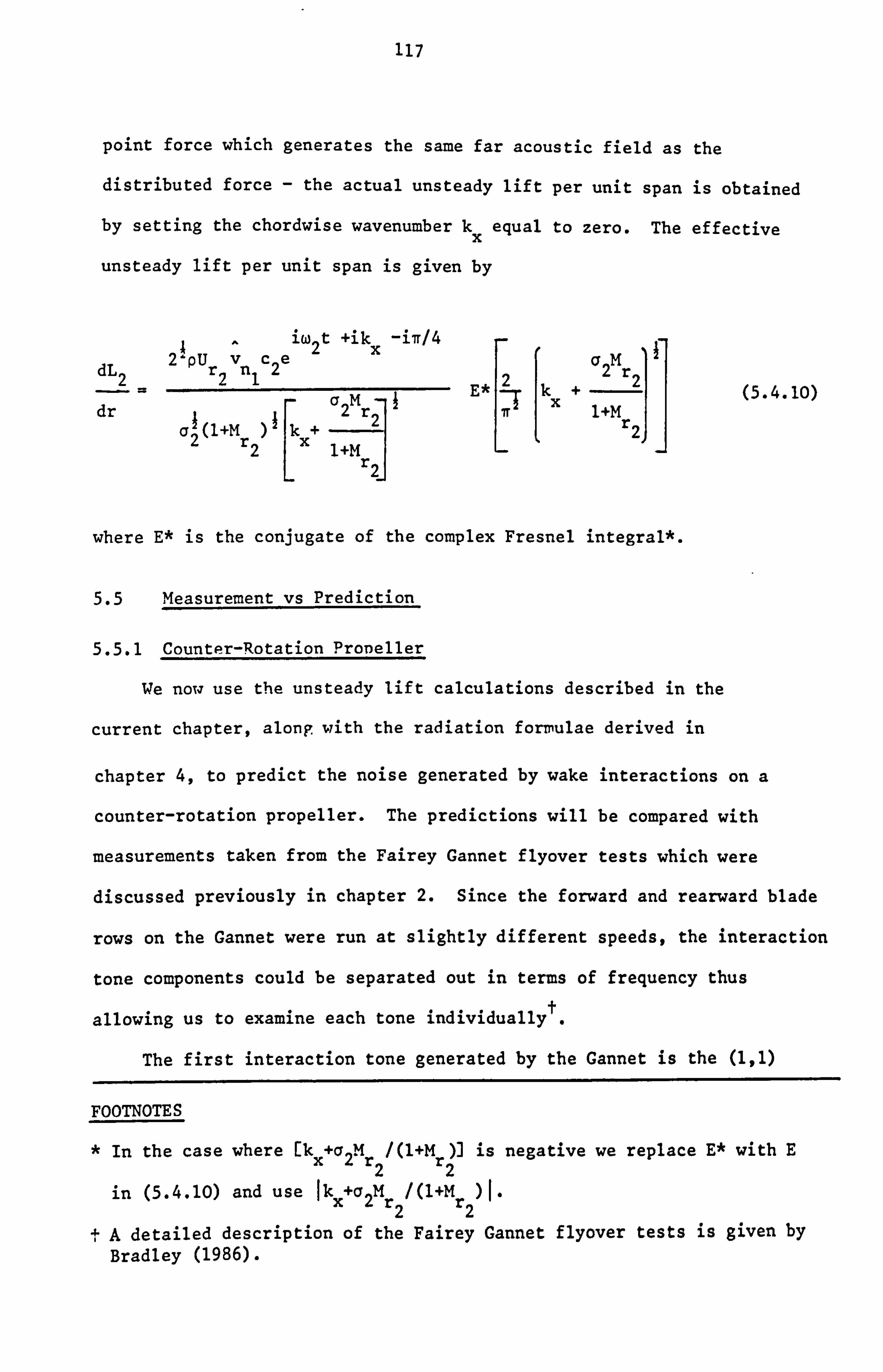
117

point force which generates the same far acoustic field as the

distributed force - the actual unsteady lift per unit span is obtained

by setting the chordwise wavenumber kX equal to zero. The effective

unsteady lift per unit span is given by

I iw2t +ikx -i7r/4

dL 2`pUr vn c2e 221

dr Q2Mr2

Q (1+M )k+ 2 r2 x 1+M

r2

E* k+2 Tr x 1+M

r2

where E* is the conjugate of the complex Fresnel integral*.

5.5 Measurement vs Prediction

5.5.1 Counter-Rotation Propeller

We now use the unsteady lift calculations described in the

current chapter, along with the radiation formulae derived in

(5.4.10)

chapter 4, to predict the noise generated by wake interactions on a

counter-rotation propeller. The predictions will be compared with

measurements taken from the Fairey Gannet flyover tests which were

discussed previously in chapter 2. Since the forward and rearward blade

rows on the Gannet were run at slightly different speeds, the interaction

tone components could be separated out in terms of frequency thus

allowing us to examine each tone individuallyt.

The first interaction tone generated by the Gannet is the (1,1)

FOOTNOTES

* In the case where Ckx+a2Mr /(1+Mr)7 is negative we replace E* with E 22

in (5.4.10) and use IkX+a2Mr /(1+Mr )ý. 22

tA detailed description of the Fairey Gannet flyover tests is given by

Bradley (1986).

118

interaction. The directivity plot for this tone is shown in Figure 5.2.

We can see that there is a null at the 900 radiation angle in both the

measured and predicted data. This is to be expected since the (1,1)

interaction tone generates a plane wave mode (on the Gannet which has

equal blade numbers on the forward and rear rows), i. e. n1Bl - n2B2 = 0,

which peaks on the propeller axis and is zero in the plane of the rotor.

However, the predictions are, typically, 25dB below the measurements.

The next two interaction tones generated by the Gannet are the

(2,1) and (1,2) interactions for which directivity plots are shown in

Figures 5.3 and 5.4 respectively. For these interaction tones the

predictions are at least 10dB below the measurements. In fact, it is

not only the levels that are incorrectly predicted but also the

directivities: the predictions are 20dB below the measurements for the

(1,2) interaction in the forward arc; the predictions are 40dB below the

measurements for the (2,1) interaction in the rear arc*.

Bradley (1986) considered the directivities of the interaction

tones generated by the Gannet. He showed that, although the measured

directivities were similar in level in forward and rear arcs, any noise

source on the rear blade row produced only asymmetrical directivities

(except for the plane wave case where n1- n2). This result suggested

that there was a noise source on the forward blade row. In order to

generate tones at the (nl, n2) interaction tone frequencies the noise

source must be that due to the interaction of the forward blade row with

the potential field generated by the rear row. Discussion of the potential

field interactions is, however, left to chapters 6 and 7.

FOOTNOTE

* Here, we use forward arc and rear arc to denote the angular regions

00 to 900 and 900 to 1800 respectively.

119

lOdB

Figure 5.3 Gannet measurements vs predictions for the (1,2) interaction

tone.

bdS

ANGLE

Figure 5.4 Gannet measurements vs predictions for the (2,1) interaction tone.

00 4G0 800 1200 1600

120

We now discuss the results obtain using the three different wake

models described in sections 5.2 and 5.3. For the first three interaction

tones on the Gannet, shown in Figures 5.2 to 5.4, the different wake

models gave identical results. To understand the reason for this we

consider the values of the wake wavenumber and the normalised Fourier

coefficients for the Gannet. A typical value of the wake wavenumber,

as defined by (5.3.10), for the first wake harmonic on the Gannet is

kb 1,0.05*; the wake wavenumber obtained using the Reynolds wake model

(where the wake width has a different dependence on drag coefficient from

that calculated using the Schlichting and Gaussian models) differs only

slightly from this and is, typically, about 10% higher. By using the

series expansion for the Fresnel cosine integral from Abramowitz & Stegun

(1965) we find that, for small wavenumbers, the normalised Fourier

coefficients for the Schlichting wake model, defined by (5.3.12), can

be approximated by

G(kb) tit - 81

5 kb+0(k. ) . (5.5.1)

In addition, the Fourier coefficients for the Gaussian and Reynolds wake

profiles, defined by (5.3.15), can be approximated by

2

G(kb) ti 1- kb

+ 0(kb) . (5.5.2) 41n2

FOOTNOTE

* Here we have used the value of bI in the calculation of the wake wave-

number in order to obtain compatibility between the three wake models.

121

From (5.5.1) and (5.5.2) it is clear that all three wake profiles will

give almost identical results unless kb = 0(1). This shows that, for a

low blade number propeller, the different wake models will only produce

different results at high harmonics (typically, for n1 > 10). From

(5.2.31) and (5.2.44), combined with (5.3.10), we note that the

dependence of the wake wavenumber on downstream distance is given by

kb ti (X/c)1. It then follows, from the discussion above, that for kb

to be 0(1) at low harmonics on a propfan we must have (X/c) = 0(100).

We conclude that, for all practical purposes, there will be no reduction

of wake interaction noise on a propfan with increased rotor-rotor spacing;

except, perhaps, at high frequencies. A plot of predicted wake interaction

noise against rotor-rotor spacing is shown in Figure 5.5 for the first

interaction tone on a7x7 bladed propfan. The results for all three

wake models overlay identically and, in addition, it is clear that there

is no significant change in noise level with increased rotor separation,

even when the rotors are 10 diameters apart. Experimental results

obtained by Metzger & Brown (1987) confirm that there is little

dependence of propfan noise on rotor-rotor spacing.

The results discussed above appear to conflict with general results

obtained from work on fan noise where the wake interaction usually provides

the dominant noise source. In addition it is well known that turbofan

noise reduces with increasing rotor-stator separation. Accordingly, we

will use the prediction scheme described in chapters 4 and 5 to predict

the interaction noise generated by a model fan rig in order to explain

these apparent anomalies.

5.5.2 Rotor-Stator Interactions

In this section we will compare predicted wake interaction noise

levels with measurements taken from tests carried out by Rolls-Royce on

122

Z-

lOdB

0.0 2.0 4.0 6.0 8.0 10.0 Rotor-rotor spacing/diameter

Figure 5.5 Predicted wake interaction noise vs rotor-rotor spacing for the (1,1) interaction tone on a7x7 propfan.

lOdB

6.0 8.0 10.0 Rotor-rotor spacing/diameter

Figure 5.6 Predicted wake interaction noise vs rotor-rotor spacing for blade passing frequency on a 27-bladed fan rig.

0.0 2.0 4.0

123

a 27-bladed model fan rig. The tests are discussed in detail by

Schwaller et al. (1984). Since we cannot expect the far field

directivities to be the same on ducted and unducted configurations we

will compare measured and predicted sound power levels in order to

smooth out the directivity effects. In addition we consider only the

rear arc data* so that rotor blockagef does not influence the results.

Measurements taken of the wakes from the rotor suggest that the

Schlichting or Gaussian wake models are the most appropriate. (However,

these models still overpredict the wake defect velocity due to the fact

that'the effects of rotor swirl tt

-are not taken into account. )

The predictions of interaction noise at the first two harmonics of

blade passing frequency for the three wake models, relative to measurements,

are shown in Table 5.2. Clearly, the Schlichting and Gaussian wake

Wake Models used in Prediction

Reynolds I Schlichting I Gaussian

Harmonic of 1 1.5 5.1 4.8 Blade Passing Frequency 2 -13.6 -1.0 -1.2

Table 5.2 Predicted PWL levels, relative to neasurernents, for

the Rolls-Royce'27-bladed fan rig.

FOOTNOTES

* Rear arc data refers to measurements taken of the noise radiated from the rear of the fan rig (downstream of the stators).

t Acoustic duct modes which rotate in a direction counter to that of the rotor can be reflected back along the duct instead of propagating through the rotor; for a more detailed discussion of this phenomenon see Philpot (1975).

ttOn turbofan rotors the effect of blade camber is to change the direction

of the airflow through the blade passages. The fluid then has non zero velocity in the direction of blade rotation. This velocity is termed the swirl velocity. On propfans swirl can, to a large extent, be

neglected due to the low blade camber.

124

models produce similar interaction noise levels and agree with the

measurements to within 5dB at blade passing frequency and to within

1dB at twice blade passing frequency. Since, as we commented above, the

Schlichting and Gaussian wake models also provide the best agreement with

the measured wake data, we can have some confidence in the prediction

scheme for wake interaction noise. The Reynolds wake model produces

noise levels which agree with the measurements to within 2dB at blade

passing frequency but underpredicts by nearly 15dB at twice blade

passing frequency. We now discuss the reasons for the difference in

noise level obtained using the Reynolds wake model and either the

Schlichting or Gaussian wake models.

Typical values of the wake wavenumber for the first wake harmonic

on the fan rig are kb "1 for the Schlichting or Gaussian wake models,

and kb ti 1.6 for the Reynolds wake model. The wake wavenumbers are

much higher than those on the Gannet due to a higher number of blades

(27 as opposed to 4) and higher section drag coefficients (typically 0.04

as opposed to 0.007). We can, therefore, no longer use the low wavenumber

approximations to the normalised Fourier coefficients given by (5.5.1)

and (5.5.2). Instead we must use the full expressions (5.3.12) and

(5.3.15). A plot of the variation in noise level with increased rotor-

rotor spacing, as predicted using the three wake models, is shown in

Figure 5.6. From (5.3.10) this can also be viewed as a plot of the

2 variation in noise level with kb (since b ti X'). We see that the

Reynolds wake model produces a greater decay in noise level with kb than

either the Gaussian or Schlichting models which produce similar noise

levels. However, at large rotor-rotor spacing, corresponding to kb '6

125

for the Gaussian or Schlichting wake models, the Gaussian wake model

continues to produce noise levels which decay rapidly with wake wave-

number, but the decay in noise levels obtained using the Schlichting

wake model is less rapid and tends to oscillate with wavenumber. The

Reynolds and Gaussian wake models both produce noise levels which decay

with wake wavenumber according to (5.3.15)*. The asymptotic Fourier

coefficients for the Schlichting wake model are calculated in appendix

5.1 where it is shown that

l0 ýr G(kb) ti 3 2 52 lc

b as lcb -º co . (5.5.3)

This explains why the interaction noise levels obtained using the

Schlichting wake model decay only weakly at high wake wavenumbers, At

these high wake wavenumbers the Fourier coefficients for the Schlichting

wake profile are dominated by the contributions from the edges and the

centre of the wake (where there is a discontinuity in the second

derivative). In this wavenumber regime, therefore, we must view these

rather artificial predictions with considerable caution. However, for

current technology, low drag, fans it is unlikely that the wake wavenumbers

will be high enough, in the audible frequency range, to enter this regime.

FOOTNOTE

* In (5.3.15) we must remember that the Reynolds wake is wider than the Gaussian wake, so that kb is larger.

126

APPENDIX 5.1

Fourier Coefficients for the Schlichting Wake Model

From (5.3.9) the Fourier coefficients for the Schlichting wake

model are defined by

1i

G(kb) = 10 [1

- IýI3/2 2 l

e-1 (A5.1.1)

9lJ -1

where the factor 10/9 is a normalising factor chosen so that G(0) = 1.

We rewrite (A5.1.1) in the form

G(kb) = ?0 (I1 - 212 + I3) (A5.1.2) 9

where 1

I1 Jcos kbý dý , (A5.1.3)

0

1

I2 aJ X3/2 cos kb* day , (A5.1.4)

0

I3 = j13

cos kb* day . (A5.1.5)

0

The first integral II can easily be evaluated as

sin 1% Ia (A5.1.6) 1k"

127

The third integral can be evaluated by repeated use of integration by

parts leading to

sin lcb 3cos kb 6sin kb 6 I3=

kb+ ý2 -

k3 +4(1-coslcb) (A5.1.7)

In the second integral 12 we substitute p= 7192/21% and again use

repeated integration by parts. We then obtain

sin lcb 3 cos kb 3} 2kb I2 =+ -- 2-2C

(A5.1.8) kb 2 kb 2kb

ti

7r

where C is the Fresnel cosine integral. From (A5.1.2) and (A5.1.6) to

(A5.1.8) we find that the normalised Fourier coefficients are given by

2 2kb G(kb) =

404 (1-cos kb - kbsin kb) +C (A5.1.9) 3kb 2 21cb ýr

When kb is large we can use the large argument form of the Fresnel

cosine integral from Abramowitz & Stegun (1965) which leads to

G (k_) ti 10

b32 1

mag -ºý, (A5.1.10)

Note that this result can also be obtained directly from (A5.1.1) by the

use of asymptotic Fourier transforms as described by Lighthill (1958).

128

6. POTENTIAL FIELD INTERACTIONS - INCOMPRESSIBLE FLOW

6.1 Introduction

In chapter 5 we calculated the unsteady flow generated by the

wakes shed from the upstream blades of a counter rotation propeller

and the response of the downstream blades to each convected gust

harmonic. Comparisons between the predicted far-field noise and

measured Gannet data showed that not only were the predictions

substantially below the measurements, by about 20dB in general, but

also that the directivity was incorrectly predicted, resulting in under-

predictions of about 50dB at some angles. Now, as we have mentioned

previously, the forward and rearward rows of the Fairey Gannet propeller

were run at slightly different speeds so that the different interaction

tone components could be separated in terms of frequency. Bradley (1986)

has shown that, for a specific interaction component, unsteady interaction

noise sources on the forward blade row generate directivities different

from those of unsteady interaction noise sources on the rear blade row.

The only way the gross underprediction of the Gannet data can be reduced,

therefore, is to introduce an unsteady interaction noise source on the

forward blade tow, namely that due to the interaction of the forward

blades with the bound potential field (bound vortex and thickness fields)

generated by the downstream blade row. It seems appropriate to include,

in addition, the interaction of the downstream blades with the bound

potential field generated by the forward blade row, because that is

likely to generate at least as large a field as that from the interaction

of the forward row with the potential field of the rear row - the latter

involving a trailing edge (weakly loaded if a Kutta condition is

satisfied), the former a leading edge (highly loaded).

129

In the previous chapter the flow was modelled as compressible

throughout and the response of the downstream blades was calculated as

though they were semi-infinite flat plates. Here, however, we must

consider the response of both upstream and downstream airfoils. If,

in calculating the response of an upstream airfoil, we retain the semi-

infinite flat plate model then the airfoil is extended to upstream

infinity; consequently it has no leading edge and therefore there can

be no inverse square root singularity in the response. (The inverse

square root singularity at the trailing edge is removed by the application

of a Kutta condition. ) The neglect of the standard leading edge

singularity may influence the results. Since the response of a finite

airfoil in compressible flow can only be calculated numerically it is

difficult to determine the importance of the leading edge region. We

will therefore proceed as follows.

For the present we, assume the flow to be incompressible. Then the

finite airfoil response can be calculated exactly. We can therefore

compare the results from the semi-infinite airfoil high frequency

approximation and the finite airfoil calculation in order to see whether

the leading edge inverse square singularity influences the far-field

noise. The extension to the compressible flow case will then be made

in chapter 7 where we will take account of the results from the

incompressible flow case.

In sections 6.2 and 6.3 we describe the bound potential field about

each row of a counter-rotation propeller, in incompressible flow, due to

blade thickness and blade circulation respectively. The potential field

of each row is written in terms of harmonic components.

Next, in sections 6.4 and 6.5, we consider the response of upstream

and downstream semi-infinite flat plates to each harmonic of the potential

field generated by the downstream and upstream blade rows respectively.

130

As in chapter 5 we use the Wiener-Hopf technique in order to calculate

the airfoil respcnse. A Kutta condition is imposed at the trailing

edge of the upstrean plates. The response of a finite airfoil is

described in section 6.6.

A comparison is then made between the finite airfoil and semi-

infinite plate results, in the limit of large chord, in section 6.7.

We show that, although the unsteady pressures match near the trailing

edge* in the two cases, the total unsteady lift differs by a factor of

ff/4; the lift on a finite chord airfoil being lower.

In section 6.8 we compare far-field acoustic predictions with

measured Gannet data. It is clear that the potential field interactions

produce substantially higher noise levels, for the first few interaction

tones, than the wake interactions. The differences between the finite

airfoil and semi-infinite airfoil predictions ar-^ discussed, both by

reference to the high frequency asymptotic limits, calculated in section

6.7, and the low frequency asymptotic limits, calculated in appendix 6.7.

6.2 Potential Field due to Blade Thickness

6.2.1 Velocity Potential

In order to calculate the potential flow about a blade row we

consider the thickness and lift problems separately (see, for example,

page 86 of Ashley & Landahl (1965)). In this section we discuss just

the thickness problem.

We will assume that the airfoil cross section of the blades can be

FOOTNOTE

* Here we are considering an interaction between an upstream blade and the potential field of the downstream row.

131

approximated by an ellipse of major axis b and minor axis a (see

Figure 6.1). In appendix 6.1 we show that the potential field about

the ellipse, in a uniform flow of speed Ur parallel to the major axis,

can be approximated by

Cosa -Urx -U r a(a+b)

L (Rý) 2 ax

(6.2.1)

-s ina -Ury -U ra (a+b) a (tad

2 ay

where R= (x2 + Y2)l and the coordinates x and y are shown in Figure 6.1.

The angle a in (6.2.1) represents the blade stagger angle. On taking the

Laplacian of (6.2.1) we obtain

02ý -Ur a (a+b)

Cosa a-

sinn a V2(InR)

2 ax ay (6.2.2)

= rU r a(a+b)Ccosa S'(x)S(y) - sina S(x)S'(y)]

where ö(x) is the Dirac delta function and the primes denote differentiation

with respect to argument.

In the case of an infinite cascade of airfoils, centres a distance

s apart, we obtain

132

V

U r

X

Figure 6.1 The cross section of each blade is represented by an ellipse of minor axis a and major axis b.

"I, - 2nr B2

C1

xi ty

a2

Y1 Yl

2nr B1

" 8

Figure 6.2 Coordinate systems for the interaction of the rear row potential field with the front row blades.

133

v2ý _ irUra(a+b) Ccosa V(x) 6(y"-ns) n=-ý

(6.2.3)

-sins ö(x) 5'(y-ns);.

Now, by Poisson's summation formula (see, for example, Lighthill (1958))

we know that

a(Y-ns) =1L exp -i27r n. (6.2.4)

n=-ý s n=-- s

and, by differentiation, that

00 00 2 d'(y-ns) = ii

n exp -i21r (6.2.5) n=-ý s n--c-

We can then write (6.2.3) in the Fourier series form

ICosa 61(x) +s i2nn

sins d(x) 2ý _ 7rUr a(a+b) io

s n=-ý

(6.2.6)

exp -i27rn X

s

We try to obtain a solution to (6.2.6) in the form

134

nU a (a+b) e=rj Ex1sgn(x) + A2]

s n=-ý

exp -2nI nI IAI

- i2irn , ss

where al and X2 are to be determined. On calculating the Laplacian of

(6.2.7) and equating the coefficients of 5(x) and d'(x) with those in

(6.2.6) we obtain

(6.2.7)

a

cosa 1' 2

-i sgn(n)sina 2a2 (6.2.8)

so that 0 is given by

7rU a (a+b) 0rI [cosa sgn(x) -i sina sgn(n)]

2s n--

exp -2n ln lJ .L -i2nn Y

ss

6.2.2 Upwash on Upstream Airfoil

(6.2.9)

We now consider an isolated airfoil situated upstream of the cascade.

The situation is shown in Figure 6.2. The upwash normal to the airfoil

is given by

u1 a -sina1 ai + coso; 1 '. (6.2.10)

ax ay

135

where al is the stagger angle of the airfoil. In (6.2.9) we replace

a with a2, Ur with Ur ,n with n2, etc. (where the suffix 2 is used to 2

denote values associated with the downstream blade row of a counter-

rotation propeller, which is represented by the cascade). We take n2 to

be positive (it is clear from (6.2.9) that for n2 negative the result is

just the complex conjugate of that for n2 positive) and x to be negative

(in the upstream direction). Then, from (6.2.9) and (6.2.10),

irr 2Ur2a2 (a2+b2) 2 rtn2

ul =2 n2exp (x2-iy2) + i(a2-ai) s2 n2=-ý

[-S2

(6.2.11)

We now define two new coordinate systems, (xl, yi) and (X1, Y1), as

shown in Figure 6.2. The coordinates xl and yl are measured parallel to

x and y with their origin located at the trailing edge of the upstream

airfoil. The coordinates XI and Yl are measured parallel and normal to

the upstream airfoil and their origin is also located at the trailing

edge of the airfoil. Since the upstream airfoil represents a blade on

the forward row of a counter-rotation propeller it must, of course,

rotate. Similarly, the downstream cascade, which represents the rear

row of a counter-rotation propeller, must also rotate. Specifically,

the upstream airfoil moves in the negative y direction, with velocity

r2l, and the cascade moves in the positive y direction, with velocity

rSI 21 where SIl and f22 represent the angular speeds of the forward and

rear rows and r is the radial station under consideration. The (x, y)

and (xl, yl) coordinate systems are related by

136

x x1 - (g - c1/2 cos a1),

(6.2.12)

y= y1 +c1 /2 s ina 1-r (S21 + S22) t

where cl is the chord of the upstream airfoil and g is the distance

(the "gap") between the midchords of the upstream and downstream

airfoils. The (xl, yl) and (X1, Y1) coordinate systems are related by

xl = XiCosa l- Ylsinal

(6.2.13)

yl = Xlsina1 + Ylcosa1 .

The cascade spacing s2 is given by

2nr s2= --

B2 (6.2.14)

where B2 is the number of blades on the downstream blade row. The

upwash in (6.2.11) can then be written in the form

ul = v1 exp[y1(X1-iY1) + iw1 t] (6.2.15) n2a-co

where 2 -ia in2B2Ur2a2(a2+b2)

n2B2 c 1e 1

vl 2 exp -g-+ i(a2 al) 4r r2

(6.2.16)

137

n2B2 -ia1 yl =e (6.2.17)

r

and wl is the angular frequency given by

wl = n2B2(c21+Sl 2) . (6.2.18)

6.2.3 Upwash on Downstream Airfoil

Here we consider an airfoil situated downstream of the cascade.

The situation is the same as in section 5.4 and is shown in Figure 5.1.

The upwash normal to the airfoil chord is given by

u2 = sina2 a+

cosa2 4

ax ay (6.2.19)

where a2 is the stagger angle of the downstream airfoil. (Note that, as

in the previous section, the suffices 1 and 2 are used to denote values

associated with the upstream and downstream airfoils respectively). In

(6.2.9) we replace a with -a 1 (since the cascade is now staggered in the

opposite direction to that considered in section 6.2.1) and n with -n1

(since the cascade rotates in the opposite direction to that considered

in section 6.2.1). We take n1 to be positive (as commented previously,

we can take complex conjugates for n1 negative) and x to be positive (in

the downstream direction). Then, from (6.2.9) and (6.2.19),

i7rUr al(al+bl) -2nn u2 a1 n1exp 1 (x-iy) + i(02-al

2 nl=-ý S Si 1

(6.2.20)

138

The cascade spacing s1 is given by

2rr sl = (6.2.21)

B 1

where BI is the number of blades on the downstream row. On introducing

the coordinate systems (x2, y2) and (X2, Y2), which are defined by (5.4.1)

and (5.4.2) and are shown in Figure 5.1, the upwash in (6.2.20) can be

written in the form

Co u2 v2 exp[Y2(X2-iY2) + iw2t] (6.2.22)

n1=-Co

where

2ý is in1BlUrlal(al+b1) [n1B1

c2e 2

v2 =2 exp 8-+ iia2-al) , (6.2.23) 4r r2

-n1B1 e ia2

Y2 (6.2.24) r

and w2 is the angular frequency given by

w2 m n1B1(a1+n2). (6.2.25)

6.3 Potential Field due to Blade Circulation

6.3.1 Stream Function

In section 6.2 we calculated the flow about a blade row due solely

to thickness effects, i. e. the blades were assumed to be operating at zero

139

angle of attack, and also calculated the resulting upwash on an upstream

or downstream airfoil. To complete the formulation we now need to

consider the lifting flow about a row of flat plates (airfoils of

infinitesimal thickness) operating at an angle of attack.

A flat plate operating at incidence to the mean flow generates lift

which, by the Kutta-Joukowski law (see, for example, Ashley & Landahl

(1965)), can be related to the airfoil circulation. We will therefore

model each section of a blade by a point vortex with the appropriate

circulation.

In terms of the stream function ý, the x and y components of the

velocity field are

ux ay

, uy ax

(6.3.1)

where the coordinate system is shown in Figure 6.3. It follows that for

an infinite row of point vortices, each of circulation r, situated at

x=0, y9 ns where n is any integer, * must satisfy

v2ý -r a(x) 1 6(y-ns) . (6.3.2) n=-ý

From (6.2.4) we can rewrite this in Fourier series form as

02ý a-r d(x) exp -i2nn Z, ]

- (6.3.3)

s n=-ý s

140

S= 2Trr

By

r -, 4ý

r

n Figure 6.3 The potential field due to blade circulation can be modelled by replacing each blade section with a point vortex having the same circulation.

Im s

to s A1

Figure 6.4 Contour used to evaluate the integral in (6.7.3).

141

The solution to (6.3.3) then follows immediately as*

Co =r i1 exp-2nlnl

'x' .. -i2Trn

4Tr n=- Ini s


(6.3.4)

We now consider an airfoil situated upstream of the cascade: the

situation is shown in Figure 6.2. The up wash normal to the airfoil

is given by

ul = -sina1 3*

-cosal a-

ay ax (6.3.5)

where al is the stagger angle of the airfoil. By following the analysis

in section 6.2.2 we find that the upwash normal to the airfoil can be

written in the same form as (6.2.15), with (6.2.16) replaced by

-rB2 vl exp

[-n2B2

g-- Cl

e-ial -ice (6.3.6) 4 irr r2


Here we consider an airfoil downstream of the cascade as shown in

Figure 5.1. The upwash normal to the airfoil is given by

FOOTNOTE

* It is to be understood that the summation given in (6.3.4) does not include the n=0 contribution which is, in fact, given by -rlxl/2s. The n=0 term represents the steady component (both spatially and temporally) of the velocity field and therefore has no influence on the unsteady lift to be calculated in sections 6.4 to 6.6.

142

u2 = sina2 a-

cosa2 9ý

ay ax (6.3.7)

where a2 is the stagger angle of the downstream airfoil. By following

the analysis in section 6.2.3 we find that the upwash normal to the

airfoil can be written in the same form as (6.2.22), with (6.2.23)

replaced by

rBl FU1B1

c2 ia2 v2 = exp g--e+ ia2 (6.3.8)

4nr Lr 2

6.4 Response of Upstream Airfoil (Semi-Infinite)

In this section we consider the response of the upstream blades to

the potential field generated by the rear row. Recall that (as we

commented in the introduction to this chapter) the incompressible flow

modelling of the potential field interaction in the current chapter is,

in fact, just a prelude to the compressible flow model which will be

discussed in chapter 7.

In the compressible flow case, as we found in chapter 5, the

response of an airfoil to a gust cannot be calculated exactly in the

general case (unless we use the numerical work of Graham (1970) or

Adamczyk (1971)), but can only be given in the high frequency asymptotic

limit*. For the interaction between the potential field of the downstream

FOOTNOTE

* The response can also be given in the low frequency asymptotic limit (see section 7.7).

143

row and an upstream blade the high frequency approximation can be

interpreted physically as saying that the pressure oscillates rapidly

away from the trailing edge and is, to a large degree, self-cancelling.

The response should therefore be dominated by contributions from the

trailing edge region (where the pressure is not simply a rapidly

oscillating wave with slowly changing amplitude and phase) so that the

blade can be modelled by a semi-infinite flat plate. The one area of

concern in this model is the standard leading edge inverse square root

singularity which has been thereby suppressed and, without resorting

to a numerical solution, there is no exact way to assess the importance

of this singularity in the compressible flow case.

In the incompressible flow case, however, the response of both

finite and semi-infinite airfoils can be calculated. We can therefore

determine, in this case, whether the leading edge provides a negligible

or a non-negligible contribution to the total airfoil response. The

results should indicate whether or not care should be taken in the

treatment of the leading edge region in the compressible flow case.

We start, therefore, with an airfoil extending to upstream infinity

and consider only the trailing edge problem. The velocity potential, 4,,

satisfies Laplace's equation

v2ý -0

with the boundary condition

(6.4.1)

Yx iwt

ae +v1e11-0; Y1 s 0±, X1 < 0. (6.4.2)

8Y1

144

Also, neglecting vortex wakes for the moment, 4, will be continuous

across Y1 = 0, X1 > 0. Since ý must be an odd function of YL this

means that

e=0; Y1 = 0, X1 >0. (6.4.3)

We now have a two-part boundary value problem. The solution is

obtained by using the Wiener Hopf technique (see, for example, Noble

(1958)). On imposing a Kutta condition at the trailing edge we then

obtain the pressure difference across the plate as*

(Y X

1+ -1- e1 1-wC-(X, )1y2] . (6.4.4) Ap(X1) _ -2ipUr

't

1 YlUrl

The total lift acting on the airfoil is obtained by integrating

(6.4.4) along the airfoil chord. There follows

iwlt

dLI -2ipUrlvle iwj -Ylc1 # lYlcl

=1+e- w(y1c1) + 2i (6.4.5) dr y Y1 r 1

where c1 is the chord of the upstream blade.

FOOTNOTE

* The use of the Wiener-Hopf technique, and the trailing edge Kutta

condition, are discussed in more detail in chapter 7.

145

In the following section we proceed to calculate the response of a

downstream blade to the bound potential field generated by the upstream

blade row.

6.5 Response of Downstream Airfoil (Semi-Infinite)

Here we assume that the airfoil response is dominated by contributions

from the leading edge so that the airfoil can be modelled by a plate

extending to downstream infinity. The flow is again taken to be incomp-

ressible. In this case the leading edge singularity will, of course, be

retained. We will not be neglecting a singularity at the trailing edge

since, in practice, the trailing edge singularity is relieved by the

effects of viscosity*.

We therefore consider just the leading edge problem. The velocity

potential, 0, satisfies Laplace's equation

02fß s0


(6.5.1)

Y X+iw t + v2e

222-0; Y2 a 0±, X2 > 0. (6.5.2) aY2

In addition ¢ is continuous across Y2 m 0, X2 < 0. Since 0 is odd in Y2

this means that

4-0; Y2 = 0, R2 <0. (6.5.3)

FOOTNOTE

* See the discussion on the Kutta condition in appendix 7.3.

146

We now have a two part boundary value problem which can be solved,

as in section 6.4, by using the Wiener-Hopf technique (see, in addition,

chapter 7). We then obtain the pressure difference across the plate as

r iw2 iw2 y X2 2 Ap(X2) = 2ipv2Ur e1+ w(iX2y2) -e -1 (6.5.4) 1

xi 2 Y2Ur y2 2

The total lift acting on the airfoil is obtained by integrating

(6.5.4) along the airfoil. The lift, per unit span, is then given by

iw2tý 2ipv ue dL2 2 r2

1+ w2 [w(icW)

-e +i dr 22

Y2Ur 22

(6.5.5)

where c2 is the chord of the downstream blade.

We have now calculated the response of upstream and downstream

airfoils to a potential field using the basic assumption that the air-

foils can be replaced by semi-infinite flat plates. In the next two

sections we will discuss the ramifications of this assumption.

6.6 Response of Finite Chord Airfoil

The response of an airfoil to a gust in incompressible flow is

usually calculated by way of the Sears function (see Von Karman & Sears

(1938) and Sears (1940)). However, since the potential flow field is not

convected with the mean flow we cannot use directly these standard results.

147

Instead we use the results of Kemp (1952) who made the appropriate

extensions to the response calculation for a gust moving at a velocity

different from that of the mean flow.

We rewrite the gust velocity on Y1=0 in the form

u= wIexp(iwlt -iv 1X1) (6.6.1)

where wlis the normal gust velocity at the mid chord. The relationship

between wIand v1 is therefore

-Ylc1/2 wl vIe

In (6.6.1) u1 is the normalised gust wavenumber

C1 u1a iy

1-

2

and X1 is a normalised coordinate which is related to XI by

_X X1= 1

+1 . cl/2

(6.6.2)

(6.6.3)

(6.6.4)

The unsteady pressure distribution on the airfoil in incompressible

flow, due to the gust defined by (6.6.1), is given by Anriet (1973) as*

FOOTNOTE

* We note that the response of an airfoil to a completely arbitrary upwash is given in integral form in chapter 13 of Ashley & Landahl (1965).

148

1_; 1

Ap(X1) = 2pUr wl _ 1 1+X1

CC(Q1)(Jo(in) - iJ1(u1)) + i31(u1)

(6.6.5)

-11- ül (1 - Y. i)

I1(X1) elwt 71

where Q1 is the reduced frequency defined by

a= W1 cl

. (6.6.6) 1U2

rl

In (6.6.5) C(Q1) is the Theodorsen function*, which is defined by

H(2) (Q ) C(Q) _ (2)

11 (2) . (6.6.7)

1 Hi (Q1) + M( (al)

where H(2)(x) is a Hankel function of the second kind of order n and

argument x. The integral Ii(X1) in (6.6.5) is defined by

1 -ill l&

Iý(X1) a_e2 dý (6.6.8) (X1-ß) (1-ý )

-1

and is to be interpreted as a Cauchy principal value integral.

FOOTNOTE

* Theodorsen (1935).

149

The total airfoil lift is obtained by integrating (6.6.5) along the

airfoil. The integrations are carried out in appendix 6.2 where it is

shown that

dLl iQ }1(A31t

dr -= 7rpc1Urlw1 C(a1)CJo(u1) - iJ1(u1)] +1 J1(u1) e (6.6.9)

ul

which agrees with the result of Kemp (1952).

In this section we have obtained expressions for the pressure and

lift, per unit span, or an airfoil in incompressible flow. In -the

following section we will examine whether these results match with those

obtained in section 6.4, for a semi-infinite airfoil, when the chord

length becomes large.

6.7 Finite Airfoil vs Semi-Infinite Airfoil

6.7.1 Pressure

In this section we will take the results from section 6.6, for a

finite airfoil, and let the chord become large. The results will then

be compared with the response calculations in section 6.4 where we

considered an airfoil extending to upstream infinity.

First we consider the unsteady pressure distribution on the airfoil,

due to a nonconvected gust, which is given by (6.6.5). We switch back

to the XI coordinate which is related to 5F1 by (6.6.4) and, in the Cauchy

integral (6.6.8), we define

&-1-- (6.7.1) c1/2

150

From (6.6.3), (6.6.4) and (6.7.1) the Cauchy integral can be rewritten

as

c

eYlc1/2

1

e-Yl 11(X1) =1 dL. . (6.7.2) 20 (ý+X1) ý1 1

cl

We now let cl -+ -. Since, from (6.2.17), the real part of yl is positive

the inverse square root singularity in the integrand at I= c1 can be -JylR

neglected since it is damped out by the exponential decay term e

The upper limit of integration can, for the same reason, be taken as

infinite. We therefore obtain

e Ylcl/2

e-Y1 c. dR 11 (6.7.3) 2 (R+R)Rý

10

This integral can be evaluated by considering the contour shown in

Figure 6.4. Here

CC1+C2+C3+C4 (6.7.4)

and, by Cauchy's theorem, the integral around C is zero since there are

no singularities within the contour. Now the integral along C4 tends to

zero as the length of the contour reduces to zero so that

151

J_+ C2 -C1 -C3

From Abramowitz & Stegun (1965)

(6.7.5)

-ilic e "1c1/2 i

= WE-(-X )Y 13

(6.7.6) 2(-X1)ß 11

^C1

where we must take

a-rg(X1) =r.

In addition

(6.7.7)

inc ey1c1/2eyIX1 I-1 (6.7.8)

2(-X 1) -C 3

The Cauchy integral corresponds to the integral along contour C2 so that,

from (6.7.5), (6.7.6) and (6.7.8),

inc ey1c1/2 YX 1Y'3 (6.7.9) I' 1 fe

11- WE-(-X 1) 1 1 2(-X1)

In appendix 6.3 we show that the factor

152

C(a) [Jo (11) -i il (ii )]+ i31611) (6.7.10)

is 0(013/2) for c1 large (here we have assumed that a1 and ul are

approximately of the same order) so that, to leading order, the unsteady

pressure on the airfoil is given by the Cauchy integral term in (6.6.5).

From (6.6.4), with c1 large,

(1-X2)1 =2 -X1

jcl

xx 1+ 1

ti 21 cl cl

(6.7.11)

The unsteady pressure difference across the airfoil can then be

approximated by

c /2 iwlt yX Ap(X1) ti -2ipUr wleY1

1e 1- 1re1 1-wC-(-X1) (6.7.12)

1 vi

From (6.6.2), (6.6.3) and (6.6.6) this reduces to

iwlt iwl Y1X1 Ap(X1) ti -2ipUr v1e1+e -w[-(-x 1) Yi] (6.7.13)

1Y lUr 1

which agrees exactly with the result for the semi-infinite airfoil, given

by (6.4.4, ), which was calculated using the Wiener Hopf technique.

6.7.2 Lift per unit Span

In section 6.7.1 we showed that the pressure distribution on a semi-

infinite plate agrees with that on a finite chord airfoil when the chord

153

is large and for points not close to the airfoil leading edge. We

now compare the total unsteady lift per unit span obtained in the two

cases.

(a) Finite Airfoil

The section lift on a finite chord airfoil in incompressible flow

was given in (6.6.9). In appendix 6.3 we show that the Bessel/Hankel

function combination (i. e. the term in curly brackets) tends to

Q -ill l+iTr/4 1-1e (6.7.14)

ul (2mu1)

as c1 becomes large. Then from (6.6.3), (6.6.6) and (6.6.9),

dL, PUrl°i i iwl iwlt

- ti Try 1+e as c -> o. (6.7.15) dr (ylc1) Yiur

1

1

(b) Semi-Infinite Airfoil

The section lift on a semi-infinite airfoil in incompressible flow

was given in (6.4.28). We consider each of the three terms in square -c

brackets in turn. The first is e Y1 1

which is, of course, exponentially

small as c1 becomes small (recall, from (6.2.26), that the real part of

Yl is positive). The second term is shown by Abramowitz & Stegun (1965)

to be OC(y1cl)-17 as c1 + co. The third term is obviously OE(y1cl)'],

and is therefore the leading order term. We then have

dL pUr °lcl 1

ti 41

iw

e 1Wlt

as cl (6.7.16) dr (y1c1) Ylu

1)

154

By comparison with (6.7.15) we see that the total unsteady lift per unit

span on a large, but finite, chord airfoil is n/4 times that on the

equivalent length cl, as measured upstream from the trailing edge, of a

semi-infinite airfoil. In section 6.7.1, however, we found that the

pressure distribution was the same in both cases. We will now discuss

this apparent anomaly in more detail.

6.7.3 The Factor of 7/4

The two expressions, (6.7.15) and (6.7.16), show that the total

unsteady lift on an airfoil section does not converge with increasing

chord length; in fact the lift diverges as cl. It follows that the

leading edge portion of the blade is important, even when the unsteady

flow field decays exponentially with distance, as was the case here. In

the analysis carried out in section 6.7.1 we made a number of approximations

involving the leading edge portion of the airfoil. These approximations

will now be reviewed.

In (6.7.2), the vorticity integral Ii was approximated by neglecting

the inverse square root singularity at the leading edge and extending the

upper limit of integration to infinity. These steps are certainly

justified since there is an exponential decay factor under the integral

sign which damps out the leading edge contribution. A second approximation

was made in (6.7.11) where, essentially, we assumed that X1/cl « 1.

Near the leading edge, however, X1/c1 ti 1 and we have shown that the

leading edge region provides a non-negligible contribution to the total

airfoil lift. We must therefore retain the factor (1 + X1/c1) in (6.7.11).

The effect of the factor (1+ X1/c1)1 is to reduce the unsteady

pressure difference across the airfoil to zero, parabolically, at the

0

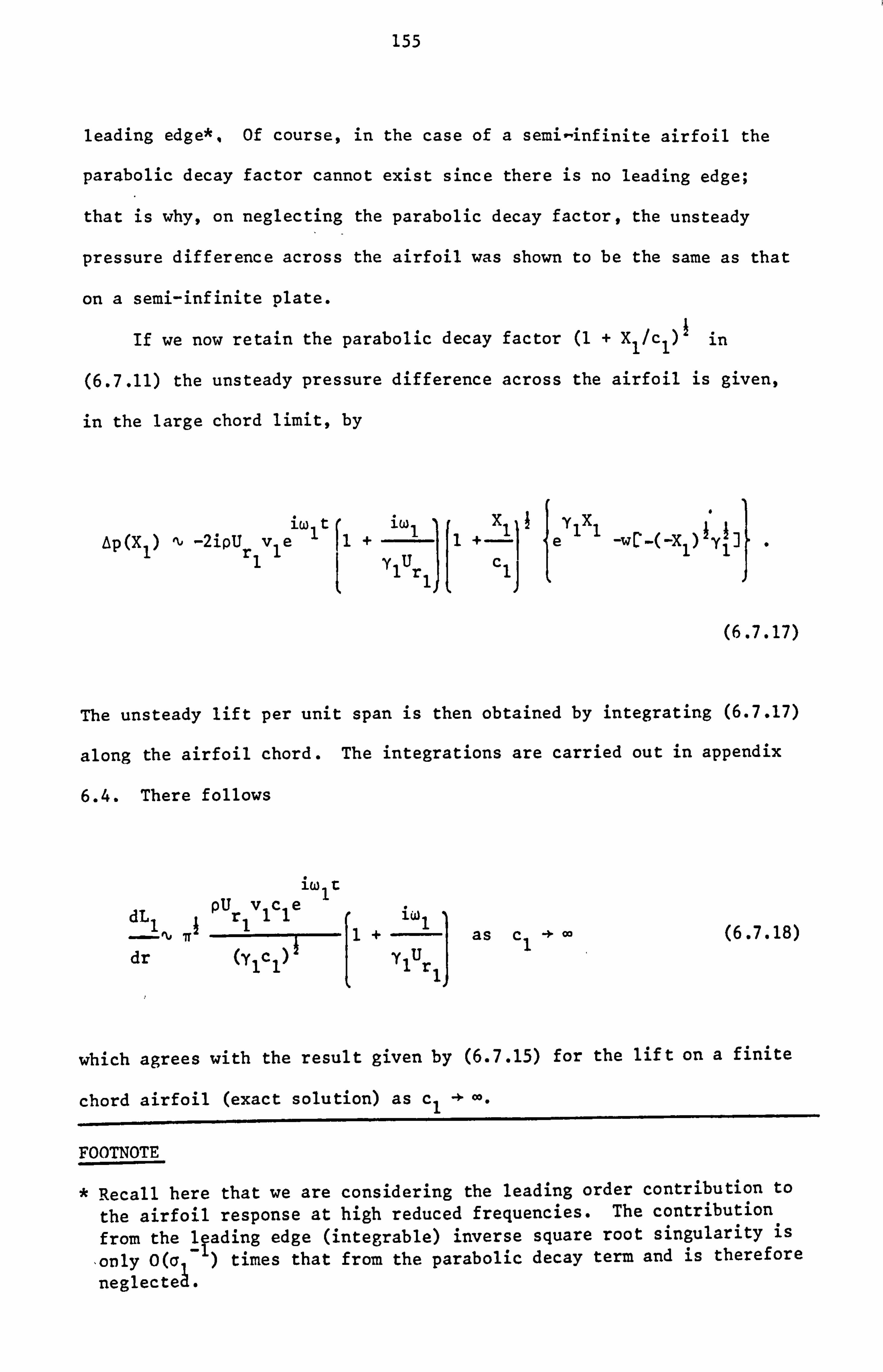
155

leading edge*, Of course, in the case of a semi-infinite airfoil the

parabolic decay factor cannot exist since there is no leading edge;

that is why, on neglecting the parabolic decay factor, the unsteady

pressure difference across the airfoil was shown to be the same as that

on a semi-infinite plate.

If we now retain the parabolic decay factor (1 + X1/c1)1 in

(6.7.11) the unsteady pressure difference across the airfoil is given,

in the large chord limit, by

Ap (X ) ti -2ipU ve iw

1t (1 +

1w1 1+

X 1I 1 rl 1

YlUr ell 1J

eYlXl WC-i Ry II

(6.7.17)

The unsteady lift per unit span is then obtained by integrating (6.7.17)

along the airfoil chord. The integrations are carried out in appendix

6.4. There follows

dL1 I PUrlv1c1e

iU)l t iwl

ti --ýý- 1+ as c 00 (6.7.18) dr (Ylcl) I lur

1

which agrees with the result given by (6.7.15) for the lift on a finite

chord airfoil (exact solution) as cl - 00.

FOOTNOTE

* Recall here that we are considering the leading order contribution to

the airfoil response at high reduced frequencies. The contribution from the ltading edge (integrable) inverse square root singularity is

, only 0(Ql ) times that from the parabolic decay term and is therefore

neglected.

156

The results of this section show that, in incompressible flow, the

airfoil cannot accurately be modelled by a semi-infinite plate; even

though the two solutions for the resultant unsteady pressure difference

across the airfoil agree precisely except in the region of the leading

edge. The reason for this is that the trailing edge region does not

dominate the unsteady lift induced by the gust and the two solutions,

for a finite and a semi-infinite airfoil, produce different unsteady

pressure distributions in the region of the leading edge*: in the case

of the finite airfoil the pressure drops parabolically to zero at the

leading edge when the chord is sufficiently large (or, as is appropriate

here, the gust frequency is sufficiently high); in the case of the semi-

infinite airfoil there is, obviously, no leading edge and the unsteady

pressure just decays as (-X1)-' away from the trailing edge. The

difference in pressure distributions near the leading edge in the two cases

wholly accounts for the factor of w/4 between the lift on the trailing

edge region, of length cl, of a semi-infinite airfoil and that on a

finite airfoil of length cl.

For a downstream gust interaction problem in incompressible flow

the same result holds; for either convected or nonconvected gusts (i. e.,

for wake or potential field interactions). In this case a Kutta condition

is imposed at the trailing edge of the finite airfoil so that the unsteady

pressure drops to zero there. The semi-infinite airfoil has no trailing

edge and, as in the previous case, the pressure will just decay as X2

away from the leading edge. This difference in the trailing edge behaviour

again results in a factor of w/4 between the lift on the leading edge region,

FOOTNOTE

* For the semi-infinite airfoil the leading edge is represented by the

point X1= -cl.

157

of length c2, of a semi-infinite airfoil and that on a finite airfoil

of length c2.

The main approximation made in the current section (and, indeed,

in the whole of the current chapter) is the assumption of incompressible

flow. This implies that the sound speed is infinite, so that a disturbance

at the trailing edge of an airfoil is felt immediately at the leading

edge. In practice, since the sound speed is finite, there is a time

delay of cl/(co-Ur ). In order that the phase difference between leading

edge and trailing edge is not significant the time delay should be small

in comparison to the period 21T/c, l" Amiet (1973) suggests a fraction of

1/r as appropriate so that, for reasonable accuracy, we require

a1Mr 1<1.

1-M r1

(6.7.19)

This means that, even if the Mach number is small, the incompressible

flow assumption will produce inaccurate results for high reduced

frequencies (i. e. large chord or high frequency). The semi-infinite

airfoil assumption will, therefore, only produce the correct response

at distances from the trailing edge compatible with (6.7.19), as was

shown by the agreement between (6.4.27) and (6.7.13). We note that,

in a discussion of the unsteady Kutta condition , Daniels (1978) found

that in incompressible flow the unsteady pressure difference across an

airfoil grew algebraically at large distances upstream from the trailing

edge. Daniels comments that in the compressible flow case (which is

considered by Crighton (1972)) the same is not true and the pressure

oscillates away from the trailing edge. However, even in compressible

158

flow, we must be careful about the behaviour at large upstream distances

from the trailing edge.

In chapter 7 we show how a trailing edge problem, in compressible

flow, can be modified to provide the correct behaviour far upstream.

The solution takes the form of an asymptotic series in increasing powers

of a'. The same procedure cannot, however, be used in incompressible

flow because then each term in the series is of the same order, i. e.

o(vl1>.


In this section we use the expressions for the unsteady lift given

in sections 6.4 to 6.6, along with the radiation formulae given in

chapter 4, to calculate the resultant far field noise. In the case of

the downstream wake interaction, which was considered in chapter 5, the

noise sources were positioned on the rearward blade row; here, however,

we have noise sources on both forward and rearward blade rows. Since

the relative phasing of the two sources must, therefore, be corrected

to account for spatial separation* we will, for the present, consider

the fields separately. Throughout the discussion we will refer back to

the results of chapter 5 to determine the relative predicted noise levels

due to potential field and wake interactions. The predictions will be

compared with the measured Gannet flyover data which were discussed in

section 2.3.

We start with the semi-infinite airfoil response calculations given

in sections 6.4 and 6.5. The first interaction tone generated by the

FOOTNOTE

* Acoustic interference between the rotor-alone tones generated by the forward and rearward rows of a counter-rotation propeller are discussed by Hanson (1985a).

159

Gannet is the (1,1) interaction. The far-field directivity of this tone

is shown in Figure 6.5. The first thing to note is that the predicted

potential field interaction noise is significantly greater than the

predicted wake interaction noise: the predicted forward and rearward

potential field interaction tones* are. tyvically. 10dB and 20dB greater

than the predicted wake interaction tone respectively. The second

important point follows directly from the first: the predicted rearward

potential field interaction noise is greater than the predicted forward

potential field interaction noise, typically by about 10dB. The predicted

rearward potential field interaction noise agrees well with the measured

data in the forward arc (0 ,0: 90°) but underpredicts by approximately

5dB in the rear arc (90° ,0; 180°). The next two interaction tones

generated by. the Gannet are the (2,1) and (1,2) interaction tones, for

which directivity plots are shown in Figures 6.6 and 6.7. Here we see

again that the predicted potential field interaction noise levels are

significantly greater than the predicted wake interaction noise levels by,

typically, 15dB (and more at some angles). Note that sources on the

forward blade row (due to the upstream potential field interaction)

generate far-field directivities different from those of sources on the

rear blade row (due to the downstream wake and potential field interactions).

This agrees with the general idea of Bradley (1986) which, as we have

mentioned, led üs to consider the potential field interactions. The

FOOTNOTE

* The forward potential field interaction refers to the interaction between the upstream blade row and the potential field generated by the rear row. The rearward potential field interaction refers to the interaction between the downstream blade row and the potential field

generated by the forward row.

160

P.. A /1`. \ lOdB MEASURED

RWD POT', \/ 'ý " ýý".

Nyf FWD POT

;1 ý\; ºfr/i 4 v If

I! ,,

; WAKE ;I ns dSi d

41, 0.0 40.0 80.0 120.0 160.0

ANGLE

Figure 6.5 Gannet measurements vs predictions for the (1,1) interaction tone. The potential field predictions are obtained using semi-infinite airfoil re§ponse'calculations. in incompressible flow.

lOdB ýý f MEASURED

/ Al%i \ý \

'// FWD Pý00T% 1

\ \\ ` ,`

V/ % 11 'If %% \

% %

iJv RWD POT\ l `\

WAKE

0.0 40.0 80.0 120.0 160.0

ANGLE

Figure 6.6 Gannet measurements vs predictions for the (2,1) interaction tone. The potential field predictions are obtained using semi-infinite airfoil response calculations in incompressible flow.

161

10dB

10dß

'I ý/ \' \

I1\

ANGLE

'--ý MEASURED oýý.

--"ýý% RWD POT

% ý %%

- 'o

f%/ \-- 1 11 i. \% %

/%

ii FWD POT Ii

WAKE

ANGLE

0.0 40.0 80.0 120.0 160.0

Figure 6.7 Gannet measurements vs predictions for the (1,2) interaction tone. The potential field predictions are obtained using semi-infinite airfoil response calculations in incompressible flow.

Figure 6.8 Gannet measurements vs predictions for the (1,1) interaction tone. The potential field predictions are obtained using finite chord response calculations in incompressible flow.

162

downstream potential field interaction is clearly the dominant source

(except for the (2,1) interaction where the forward potential field

interaction tone dominates in the rear arc) leading to good agreement

with measurements in the forward arc and discrepancies of ± 5dB

(depending on the interaction tone considered) in the rear arc.

Next we consider the finite chord calculations given in section 6.6

(these calculations are applied to both upstream and downstream potential

field interactions). The far-field directivities of the (1,1), (2,1)

and (1,2) interaction tones are shown in Figures 6.8,6.9 and 6.10

respectively. By comparison with Figures 6.5,6.6 and 6.7 we can see

that the predicted upstream potential field interaction noise levels have

increased, by about 3dB, and the predicted downstream potential field

interaction noise levels have decreased, by about 7dB, in relation to the

semi-infinite airfoil results. At first sight these results appear to

conflict with the results of section 6.7 (i. e., that the semi-infinite

airfoil model should give noise levels about 2dB above those obtained

using the finite airfoil model); however, we must remember that the

reduced frequencies of the first few Gannet interaction tones are not

high, so that the results of section 6.7, which were obtained for the

high reduced frequency limit, are not strictly applicable here. As an

aid to understanding the results we discuss the low frequency behaviour

of the airfoil response in appendix 6.5, for both the finite airfoil and

the semi-infinite airfoils. There we show that the unsteady lift on the

upstream blade row, as calculated using the semi-infinite airfoil model,

is where ul is small, times that calculated using the (exact) finite

chord model. Consequently the far-field noise calculated using the semi-

infinite airfoil model will be lower in magnitude than that calculated

163

lOdB

MEASURED

/"

ý\\

\

r, j

WAKE ºº 1ý

iý

0.0 40.0 80.0

rwu rvr

%

RWD POT ,

"

120.0 180.0


MEASURED

lOdB ýý ýý`q" 'RWD POT

FWD POT

WAKE ý, '

0.0 40.0 80.0 120.0 18.0

ANGLE

ANGLE


164

using the finite airfoil model in the low frequency limit. In addition

we show, in appendix 6.5, that the unsteady lift on the downstream blade

row, as calculated using the semi-infinite airfoil model, is O(1-2i), where

u2 is small, times that calculated using the finite chord model.

Consequently, in this case, the far field noise calculated using the

semi-infinite airfoil model will be higher in magnitude than that

calculated using the finite airfoil model in the low frequency limit.

The differences in lift are, in each case, due to leading edge effects:

for the upstream potential field interaction the finite airfoil response

has an inverse square root singularity at the leading edge (which is not

damped out by the decaying velocity field as it is in the high frequency

case) whereas the semi-infinite airfoil response contains no singularity

(there is, of course, no leading edge and a Kutta condition has been

imposed at the trailing edge); for the downstream potential field inter-

action the unsteady pressure difference across a finite airfoil near the

leading edge is O(u2) times that across a semi-infinite airfoil near the

leading edge.

These results show that for low frequency interactions in incompressible

flow the semi-infinite airfoil approximation can result in substantial

under-or over-predictions of the unsteady lift and hence in the radiated

acoustic field. The errors can be attributed to erroneous behaviour near

the leading edges of airfoils*.

For high frequency interactions in incompressible flow the semi-

infinite airfoil approximation results in overprediction of the unsteady

FOOTNOTE

* In the case of an airfoil extending to upstream infinity the leading

edge refers to the point one (real airfoil) chord length upstream from

the trailing edge.

165

lift by a factor of 7/4 and hence an overprediction of 2dB in the

radiated sound field. The overprediction of the semi-infinite airfoil

model here is entirely due to the behaviour away from the local airfoil

edge (where the unsteady pressures agree between the two models): in

the case of the finite airfoil model the pressure reduces to zero at

the furthest edge; in the semi-infinite airfoil model the pressure does

not reduce to zero but decays as 1XI-1 away from the local edge.

In the compressible flow case, which is discussed in the next

chapter, it is not possible to calculate the airfoil response exactly*

and we are forced to consider the high frequency limit. Consequently we

will need to examine the leading edge behaviour, to ensure that important

effects here are not neglected.

FOOTNOTE

* The airfoil response can, of course, be calculated exactly with a

numerical solution such as that described by Graham (1970) or Adamczyk (1971).

166

APPENDIX 6.1

The Potential Field of an Ellipse

First we define a conformal mapping from a circle of radius r in

the E plane to an ellipse, of major axis b and minor axis a, in the

z-plane (see Figure 6.11). The mapping is of the form

Z=+ 22

. (A6.1.1)

When ý=r the corresponding value of z is b and when ý= it the value

of z is ia. Using these values in (A6.1.1) and solving for r and R we

obtain

r (a + b) R2

(b 2-a2 ) (A6.1.2) 24

If we introduce flow of velocity Ur in the direction of the positive

real axis then the complex potential, in the &-plane, is given by

2 WiE) -UrUrr (A6.1.3)

(see, for example, Milne-Thompson (1948)). Far away from the origin the

inverse of (A6.1.1) is

167

a) ca Cl. N

0) cý a bP

N

1 w' N

t N +

4P

11 11

ya N

ai

N

C)

IJ

a)

a,

0

ai

a, u

C. )

E 0 $4 w to

a. ca E3

ca

0 w 0 U

v

co . -4 w

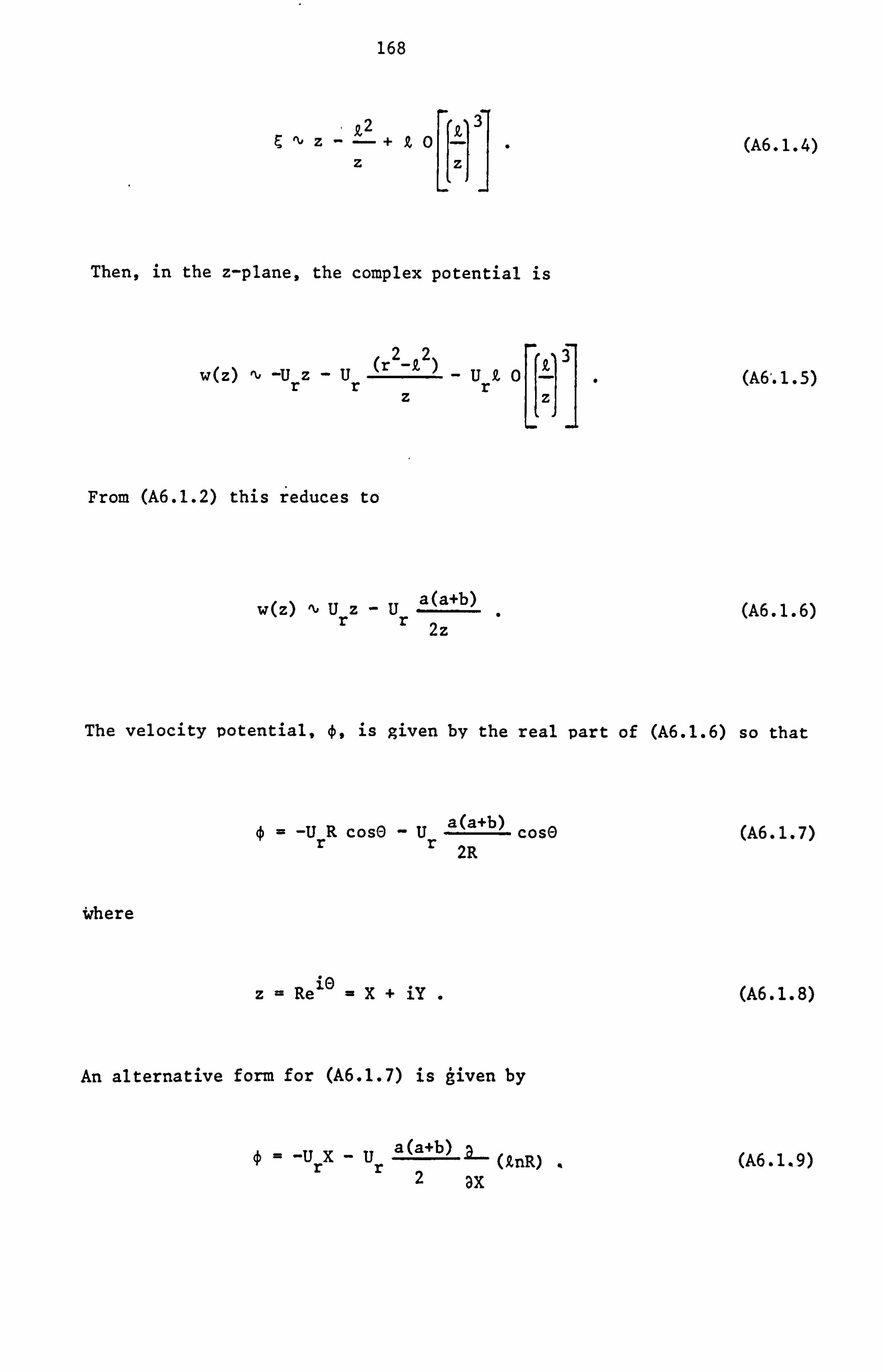
168

2 2+ X03 (A6.1.4)

z LZJ

Then, in the z-plane, the complex potential is

223 w(z) ý, -u z- ur

(r -! C )- urk 0 Z' (A6'. 1.5)

rzz

From (A6.1.2) this reduces to

w(z) ti Urz - Ur a (a+b) (A6.1.6)

2z

The velocity potential, 0, is given by the real part of (A6.1.6) so that

_ -UrR cosO - Ur a(a+b) cose (A6.1.7) 2R

where

z= Rely =X+ iY . (A6.1.8)

An alternative form for (A6.1.7) is given by

_ -Urx - Ur a(a+b) (knR) (A6.1.9) 2 ax

169

APPENDIX 6.2

Chordwise Integration (Finite Airfoil)

The pressure distribution along the airfoil is given by (6.6.5).

The total lift is therefore obtained by integrating between X1 = -1 and

X1 =1 and multiplying by c1/2 (since X1 represents distance scaled on

the semichord). We therefore need to consider the single integral

1 1-Xl _ I1 = dXl (A6.2.1)

1+X1 -1

and the double integral

1_1 lull

I= (1 - X) _e

dg dX1 . (A6.2.2) 2i (X1-9)(1-2 )

-1 -1

We now make the substitutions

%1 = -cose, _ -cos, . (A6.2.3)

The integral (A6.2.1) can then be simply evaluated as

Ii=Tr . (A6.2.4)

The second integral (A6.2.2) becomes, on interchanging the order of

integration,

170

I=1 eiu1cosý 2 1-cos20

dO d. 2 (cosh-cosh)

00

(A6.2.5)

From page 93 of Glaüert (1948) the inner integral in (A6.2.5) can be

evaluated as 2, rcosc. The outer integral then becomes

iulcos4 2

I2 = 7r I 7r

cosh e d¢ = iir J1(ul)

0

The unsteady lift on the airfoil is given by, from (6.6.5).

dL iw tI 1I1[C(i1)(J0(ii1)

dr _ pUrlwIc1e

1 -iJl(u1)) + iJ

1(u1 )7

- (1- Q1

I2

(A6.2.6)

(A6.2.7)

The result (6.6.9) then follows from (A6.2.1), (A6.2.6) and (A6.2.7).

171

APPENDIX 6.3

High Frequency Response of a Finite Airfoil

The total unsteady lift on a finite airfoil (in incompressible flow)

is given by (6.6.9). In order to approximate this at high reduced

frequencies we use the asymptotic forms of the Bessel and Hankel functions

given by Abramowitz & Stegun (1965). We then find that the asymptotic form

of the Theodorsen function is

C(a1) ti +0 (al1) as a1 -* -. (A6.3.1)

It follows that

C(Q1)[Jo(p1) -iJ1(p1)] + iQl

j (; j ti 2+

Oivll)]

[cos(p1-n/4) - icos(ij1-37r/4)] + iQl

cos(u1-3n/4) + 0(11 11) P1

2 -1 -iul+iir/4 Q iu1-irr/4 -p1 +iw/4

+1e+e + O(cy )I e- 7r; j 2u1

+ o(uil

(A6.3.2)

Now jil is defined by (6.6.3) and since, from (6.2.17), the real part of Y1

is positive we must have

172

iu e

1+0 as j1-). co . (Ab. 3.3)

Then, from (Ab. 3.2) and (A6.3.3), we have to leading order in ol* that

_iu1+iir/4

C(al)[j (p1) - iJ1(p1)] + iQl

J1( 1) ti 1- ý1 e--

P1 N1 (27rp1)

(A6.3.4)

Similarly, the Bessel function combination given by (6.7.10) becomes

2 -1 C(Q1)[Jo(N1) - jJi(p )] + iJl(ui) ti

[iPi_i/4

+ O(Q1 ) 7rN1

=0 (Qi3/2)

from (A6.3.3).

FOOTNOTE

(Ab. 3.5)

* We have assumed here that a1 and p1 are of the same order.

173

APPENDIX 6.4

Chordwise Integration (Finite Airfoil with c ->. co)

The pressure difference across an airfoil, in the large chord limit,

is given by (6.7.17). In order to calculate the total lift, per unit

span, we therefore need to consider the integrals

1 Il (1 - y)

1e11 dy (A6.4.1)

0

and

I2 =1 (1 - y)I w(-YiciY') dy . (Ab. 4.2)

0

where we have replaced X1 in (6.7.17) with -cly. We calculate I1 and 12

for y1cl large. The first integral I1 can be evaluated in terms of error

functions to give

-Y1c1 I1 1+ In

3/2e erf(iyici). (A6.4.3) Ylcl 2(Ylcl)

On using the asymptotic form of the error function from Abramowitz & Stegun -Y

(1965) and neglecting terms of 0(e 1 1) we find that

I1 =I+ DI(Ylcl)-2) (A6.4.4) Y1c1

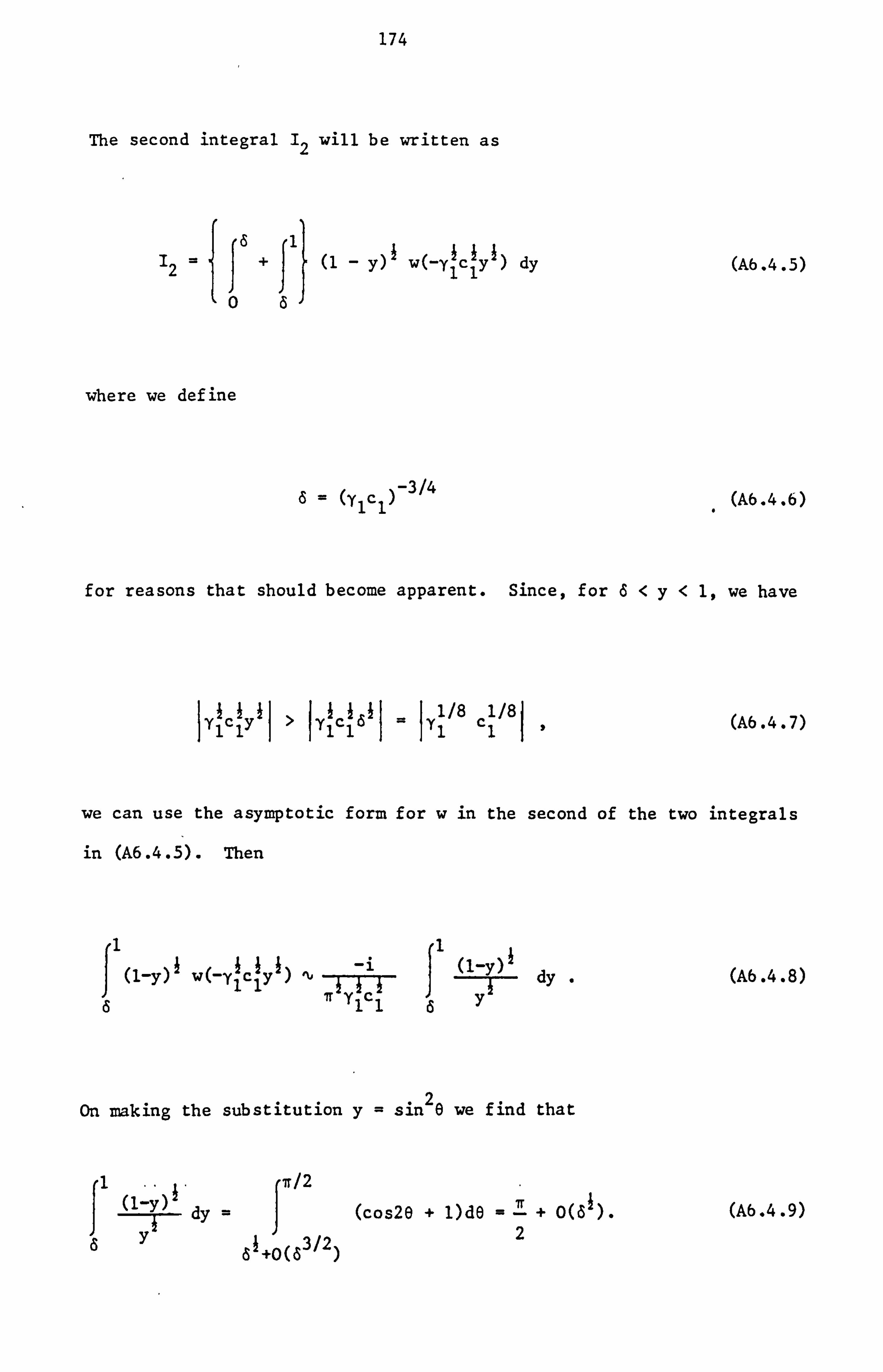
174

The second integral 12 will be written as

IsJ1 I2 =+ (1 - Y) I

w(-Yiciy') dy (Ab. 4.5)

06

where we define

6= (y, cl) -3/4 .

(A6.4.6)

for reasons that should become apparent. Since, for 6<y<1, we have

yIciy 1> 1YIC16 11

= IY1l/8

ci/81 (A6.4.7)

we can use the asymptotic form for w in the second of the two integrals

in (A6.4.5). Then

11

(1-Y) W(-YIcly ti --- dy

S116y

On making the substitution y= sin26 we find that

J1 it/2

( dy = (cos2A + 1)de =+ 0(S1). Y2

8ý+0(S3/2)

(A6.4.8)

(A6.4.9)

175

We now return to the first of the two integrals in (A6.4.5). Here we

can write

a J(i_)i w(-y clyl)dy < J+w(-y cIyl), dy sa

001 (A6.4.10)

where we have used the fact that, from (6.2.17), -yl (and hence

-yiciy' since cl and y are real and positive) lies in the upper half

plane where IwI is bounded above by 1. Combining (A6.4.5) to (A6.4.10)

we find that

I2 = 1r + O[SI(ylcl)- l+ 00) = --- -+0 (ylcl)-3/4 2y c 2y c 1111

(Ab . 4.11)

To leading order, then, the unsteady loading per unit span is, from the

above results and (A6.4.17), given by

iwlt e dLl pUrlvlc1 iwI

ti n1+ (A6.4.12) dr Ylc1 y1

r1

176

APPENDIX 6.5

Low Frequency Effects

1. Total Unsteady Lif t

]. 1 Finite Airfoil

The unsteady lift per unit span is given by (6.6.9). In order to

calculate the lift in the low frequency limit we use the small argument

Bessel and Hankel function approximations from Abramowitz & Stegun (1965).

Then the Theodorsen function can be approximated, at low reduced frequencies,

by

C(ol) ti 1. (A6.5.1)

Then, (6.6.9) reduces to

dLl ial ipl iwlt ti 7rpc Uw 'I fe (A6.5.2)

dr 1 rl 122

From (6.6.2) wl can be replaced by vl when y1cl, or p1, is small. Then,

to leading order, the unsteady lift is given by the quasi-steady approx-

imation (see, for example, section 3.4.1 of Goldstein (1976))

dLl iw t

dr ' ýpc1Urlvle (A6.5.3)

177

1.2 Upstream Semi-Infinite Airfoil

Here we use the low argument approximation to the w-function in

(6.4.5). For z small we have

w(z) ti 1+ l=- - z2 -

4iz 3 +... (A6.5.4)

rt 3ir

(it is necessary here to retain the first 4 terms). Using this

approximation in (6.4.5), with the exponential written in series form,

we find that

t

dLl -2ipUr 1vIe

iwl

ti 1+ dr Y1

iwl `

(y1cl)2 Ylcl

YlUr ý1+2

1

+ 2i(yIc1)4

-y

4i(y1c1)3/2 2i(yIc1) ý- 1c1 -

31r Ir

Then, to leading order in y1cl the unsteady lift is given by

iw iw 8t dLl

/2 1+1 (Y1cl) npclU mole

1

dr 3n YlUr r1

1

(A6.5.5)

(A6.5.6)

which is 0r. (yIc1) II or 0(u i),

times the low frequency finite airfoil

result (or quasi-steady result) given by (A6.5.3).

178

1.3 Downstream Semi-Infinite Airfoil

The low argument anpröximation to the w-function, given by (A6.5.4),

is now substituted in (6.5.5). We then obtain, on using the series form

for the exponential,

1W2t

dL 2ipv2Ur g iW r 2(y c)I 2--= 2 1+ 2 ---22 +Y2c2

dr y2 Y2Ur 2

Tr,

(d-(1 + Y2C2)

Y U2 (Y2C2)i

2 r2

(A6.5.7)

To leading order in y2c2, then, the unsteady lift per unit span is given

by

dL2 _ -4i

dr (Y2c2

i(2t 'Trpc2Ur v2e

2 (A6.5.8)

which is OE(y2c2)-1], or 0(u21), times the low frequency finite airfoil

result given by (A6.5.3)*.

2. Unsteady Pressure

2.1 Finite Airfoil

The unsteady pressure distribution across the airfoil is given by

FOOTNOTE

* For the downstream finite airfoil interaction the suffix 1 throughout (A6.5.3) is replaced with 2.

179

(6.6.5) where the singular integral Ii is defined in (6.6.8). In

(6.6.8) we will use the substitutions (A6.2.3). Then, on using the

approximation

we find that

-iu1ý e ti 1- iulý.

(1+ip1cos4) I1 ti

(cos4'-cosh) 0

dý = i1 'TT.

(A6.5.9)

(A6.5.10)

If we now substitute (A6.5.10), the Bessel function low argument approx-

imations, and the Theodorsen function approximation (A6.5.1) into (6.6.5)

we obtain, to leading order in ul,

Op(X) ti 2pUr wl _1

elft . 1 1+X 1

(A6.5.11)

To 0(ul) we can, from (6.6.2), replace w1 with vl. Then, on using the

coordinate change given by (6.6.4) we find that

iw1t -X1 4

AD (X ) ti 2pU Ve 1 rl 1 jc1+x1j (A6.5.12)

Equivalently, for a downstream finite airfoil, we obtain

180

iw2t c2-X2 Ap(X2) ti 2pUr v2e (A6.5.13)

2 X2

2.2 Upstream Semi-Infinite Airfoil

On using the low argument approximation for the w -function and the

exponential in (6.4.4) we obtain

2 iwl iwlt -X

Ap(X1) ti 1+ (y1cl) 2PUr v1e (A6.5.14) 1 cl ylUr

1

which is or (y1cl)1?, or 0(ui), times the low frequency finite airfoil

result, given by (A6.5.12), in the region of the trailing edge and has

no singularity at X1 =- cl (the leading edge).

2.3 Downstream Semi-Infinite Airfoil

The low frequency approximation to (6.5.4) is

1W2t c

Ap(X2) ti 2pUr v2e (A6.5.15) 7r (y2c2) 2 x2

which is OC(y2c2)-'], or O(i ), times the low frequency finite airfoil

results, given by (A6.5.13), in the region of the leading edge and does

not reduce to zero at X2 = c2 (the trailing edge).

181

7. POTENTIAL FIELD INTERACTIONS - COMPRESSIBLE FLOW

7.1 Introduction

In the last chapter we calculated the unsteady flow generated by

the bound potential field about the upstream and downstream blade rows

of a counter-rotation propeller, and the response of the adjacent blade

row to each harmonic of the unsteady velocity field. The calculations

were performed assuming that the flow could be considered incompressible.

This means that the modelling is inappropriate when the flow Mach

numbers are, typically, greater than 0.3 (see, for example, the discussion

on page 15 of Lighthill (1986)). Since the Mach numbers of interest on

propfans are always above 0.3*, even at approach conditions, we need to

extend the modelling in chapter 6 to include compressibility effects.

In sections 7.2 and 7.3 we describe the bound potential field about

each row of a counter-rotation propeller, in compressible flow, due to

blade thickness and blade circulation respectively. The potential field

is written in terms of harmonic components and we show how the exponential

decay of each component differs from the exponential decay given in

chapter 6 for the incompressible flow case. The upwash on the forward

and rearward blade rows, due to each harmonic gust, is then calculated.

In the case of compressible flow it is not possible to calculate

the response of an airfoil to a gust in closed form. We therefore start

by considering the high frequency limit and, in section 7.4, we calculate

the response of the upstream blades to each harmonic of the potential

field generated by the downstream row by using the Wiener Hopf technique.

FOOTNOTE

* Here the Mach number is the blade helical Mach number Mr and not the flight Mach number of the aircraft.

182

In using this technique we are assuming that the airfoil response is

dominated by contributions from the trailing edge region so that leading

edge effects can be neglected. One of the important results of chapter

6 was that the leading edge region can provide a non-negligible contrib-

ution to the total unsteady lift. Therefore, in order to account for

the leading edge effects we extend the iterative technique developed by

Landahl (1961) and Adamczyk (1974), who considered downstream convected

gust interactions, to the case of an upstream potential field interaction.

This technique provides a solution, in the form of an asymptotic series,

to a three part boundary value problem and is discussed in section 7.5.

Following on from this we discuss the high frequency response of the

downstream blades to the potential field of the upstream row in section

7.6.

Next we consider the low frequency limit and, in section 7.7, we

show that, in this limit, the compressible flow problem can be reduced to

an equivalent incompressible flow problem. The results from chapter 6

and the work of Osborne (1973) and Kemp (1973) then enable us to calculate

the total airfoil response* to each harmonic of the potential field

generated by the adjacent blade row.

In section 7.8 we compare the predicted far-field noise generated

by a counter-rotation propeller (as calculated using the radiation

formulae of chapter 4, with the unsteady lift provided by the results of

. 11 the current chapter) with the Gannet flyover measurementsI which have been

described in previous chapters and, in more detail, by Bradley (1986). The

FOOTNOTES

* When noncompactness effects are taken into account.

t In particular, we consider the first three interaction tones.

183

predictions made using the high frequency approximation are shown both

with and without a Kutta condition imposed at the trailing edges of the

blades on the upstream row. On retaining the Kutta condition, predictions

and measurements are shown to agree extremely well, typically to within

2 or 3dB. On rejecting the Kutta condition, however, the predictions are

raised by between 5 and 10dB and, in some cases, the directivity of the

far-field sound is altered. The predictions made using the low frequency

approximation are similar to those made using the high frequency approx-

imation. Since the first few interaction tones on the Gannet are basically

low frequency interactions, the equivalence of the low and high frequency

predictions for these tones suggests that only the high frequency approx-

imation need be retained.

7.2 Potential Field. due to Blade Thickness


In this section we will extend the analysis of section 6.2 to the

compressible flow case. We again assume that the airfoil cross section

of the blades can be approximated by an ellipse of minor axis a and

major axis b. The compressible flow problem can be reduced to an

equivalent incompressible flow problem by applying a Prandtl-Glauert

transformation*; see, e. g., Landau & Lifshitz (1959) or Ward (1955).

This means that the (X, Y) coordinates, which are measured parallel and

normal to the airfoil chord, are scaled according to

x' = X,

Y' = ßY, (ß. 2. i)

FOOTNOTE

* See Prandtl (1930) and Glauert (1928).

184

where

ß il - Mr (7.2.2)

and Mr is the airfoil section relative Mach number. In addition if

6' = ßýs (7.2.3)

where c is the velocity potential in the (X, Y) coordinate system, then

ý' represents an "incompressible flow" velocity potential in the (X', Y')

coordinate system about an ellipse of minor axis ßa and major axis b.

In the case of a staggered cascade of airfoils the separation s should

also be scaled according to (7.2.1). Then, by comparison with section

6.2, we find that 4' satisfies

0'2 7rUrßa(ßa+b) ZaL (X'+ns sina)6(Y'-ns ß cosa)1, (7.2.4) n=-- 8X'

where 0'2 denotes the Laplacian in the (X', Y') coordinates and a is the

airfoil stagger angle.

We now introduce the coordinates (x, y) which are measured normal

and parallel to the cascade direction and are shown in Figure 5.1. From

(7.2.1; the (x, y) and (X', Y') coordinate systems are related by

X' x cosa -y sins , (7.2.5)

Y' = ßx sina + ßy cosa .

185

This can be inverted to give

x= X'cosa + y, sins

y =-X'sina + y' Cosa

ßJ

(7.2.6)

In appendix 7.1 it is shown that the delta function combination in (7.2.4)

can be related to a delta function combination in (x, y) coordinates by

6(X'+ns sins) 6(Y'-ns ßcosa) =1 d(x)d(y-ns). (7.2.7) ß

Then from (7.2.6), (7.2.7) and the chain rule we find that (7.2.4) can be

written in the form

[coscL rUa(ßa+b) d'(x) 5(y-ns)-sina d(x)d'(y-ns)] (7.2.8)

co

n=-ý

where the primes on the delta functions denote differentiation with respect

to argument. By using Poisson's summation formula, as in section 6.2,

we then obtain

7rUra($a+b) exp(-i27rn S) s n=--

[Cosa ö'(x) + i21rn

sins d(x)]. S

(7.2.9)

186

Now from (7.2.3) and (7.2.6) the Laplacian of ý' in the (X', Y')

coordinate system can be rewritten as

0'2ý' =1 '(sin2a+ß2cos2a) a22 + 2sina cosa(1-52)

a2

s ax axay

+ (cos ta+ß2sin2 a)

92

a2 y

(7.2.10)

We will try to obtain a solution to (7.2.9) and (7.2.10) in the form

Co X0 j [x1sgn(x) + A2] exp -i27rn

y

n=-ý s

exp -2711n1 Ixl

ar - i2irn x

ss

where

Arßa(ßa + b) A=

0 s

(7.2.11)

(7.2.12)

and X1, A2, Xr and ai are to be determined. On substituting (7.2.11) into

(7.2.10) and equating the coefficients of S(x) and d'(x) with those in

(7.2.9) we obtain, after some manipulation,

Cosa (7.2.13) 1

2(sin2a + ß2cos2a)

187

_ -i sgn(n)sina A2

2ß(sin2a + 02cos2a)

r (sin2a

ß+B2

costa)

X. _ -(1-ß 2 )sins cosa

(sin 2a + ß2cos2a)

so that, finally,

irUra(ßa+b) = Cßsgn(x)cosa - isgn(n)sinal E Ey

2s(sin2a + ß2cos2a) x

where

2nß lnl lxI i27(1-ß2)nx sinacosa _ Ex a exp 22 2+ 22

s(sin a+ß cos a) s(sin a+0 cos a)

and

Ey exp 1-i27rn y

s

7.2.2 Upwash on upstream airfoil

(7.2.14)

(7.2.15)

(7.2.16)

(7.2.17)

(7.2.18)

(7.2.19)

We now consider an isolated äirföil situated upstream of the cascade.

The situation has been previously described in section 6.2.2 and is shown

188

in Figure 6.2. On following the analysis in section 6.2.2 and defining

Mach numbers in the x and y directions as

Uý r2 MX = cosa2

co - (7.2.20)

and Ur2

M= sina2, y2 c 0

where co is the speed of sound, we find that the upwash can be written

in the form

ul = v1 exp(YX X1 + yy Y1 + iw1t) (7.2.21) 11

where

_n g2 2Ura2 v=2 sina 22

(ß 2a2 +b 2

)(sina 2 -iß 2 cosa 2

)(cosa l -in 2 l) l 4r (1-ýtX)

(7.2.22) I-n

2B2 -

cl cosaI) +i

cl exp

[n2 (g sinal1 ,

r221

YX = n2B2

(11 2cosa1 - isina1) , (7.2.23)

1r

yy = ý2B2

(n2sina1 + icosal) , 1 (7.2.24)

r

189

n2 is a compressibility factor defined by

ß2 + iMxM v2

ri Z= 1-*42

x

(7.2.25)

(note that n2 +1 as MX, M Y2

- 0, i. e. as the flow becomes incompressible)

and wl is the angular frequency defined by (6.2.18).


Here we consider an isolated airfoil situated downstream of the

cascade. The situation has been previously described in section 5.4.1

(for the case of a convected gust) and is shown in Figure 5.1. On using

an analysis similar to that in section 5.4.1, and defining Mach numbers

in the x and y direction as

i1 rl

MX = cosal c

and 0 (7.2.26) U

r2 M= sinal , yi c 0

we find that the upwash on the downstream airfoil can be written in the

form

u2 = v2 exp(YX X2 + YY Y2 + iw2t) (7.2.27) 22

where

190

V2 =

n1B2Urla1(ßlal+bl)

4r2(1-MX2) (sinaI+ ißlCosa

1)(cosa2+ inlsina2)

(7.2.28)

exp ý1B1 [n1(g

- c2

Cosa 2) -i C2

sina2 r22

-n1B1 YX = (nlcosa2 + isina2), (7.2.29)

2r

-n1 B1 ly = (nlsina2 - icosa2), (7.2.30)

2r

nl is a compressibility factor defined by

ßi - iMXMy 1

ni 1-M 2

x

and w2 is the angular frequency defined by (6.2.25)

7.3 Potential Field due to Blade Circulation


(7.2.31)

In the incompressible flow case, discussed in chapter 6, the potential

flow field due to airfoil circulation was obtained by consideration of the

stream function * and the airfoils were modelled by point vortices. In

191

appendix 7.2 we show that, for a row of point vortices of circulation r

in incompressible flow, the velocity potential ý satisfies

v2ý =r d'(x)sgn(y-ns) (7.3.1) 2 n=-co

where the row of vortices and the coordinate system are shown in Figure

6.3. We now apply a Prandtl-Glauert transformation to the (X, Y) coord-

inates (see Figure 7.1) as defined by (7.2.1) to (7.2.3). In the new

(X', Y') coordinate system the position of the vortices has been altered.

We therefore introduce coordinates (X, Y) which are measured normal and

parallel to the line of vortices respectively (in the scaled, or Prandtl-

Glauert, coordinate system). The (X, Y) coordinates are related to the

(X', Y') coordinates by

X= X' cosa + Y' sins , (7.3.2)

f= -X' sins + Y' cosa ,

where a represents the angle between the two coordinate systems (see

Figure 7.1). Now the distance between adjacent vortices (in the Prandtl-

Gläuert plane), as measured parallel to the X' and Y' axes, is ßs cosa

and -s sins respectively, so that

s- s(sin2a + $2cos2a)' (7.3.3)

192

scosa

os Y\ 4Y

I ý1

ýYr

-11-X

S

I\ a

X, X'

VORTEX POSITIONS I\

VORTEX POSITIONS IN IN (x, y), (X, Y) COORDINATES COORDINATES

t

a

Figure 7.1 Vortex positions in original and transformed coordinate systems.

Re s

I Figure 7.2 The integration contour and branch cuts in the complex plane.

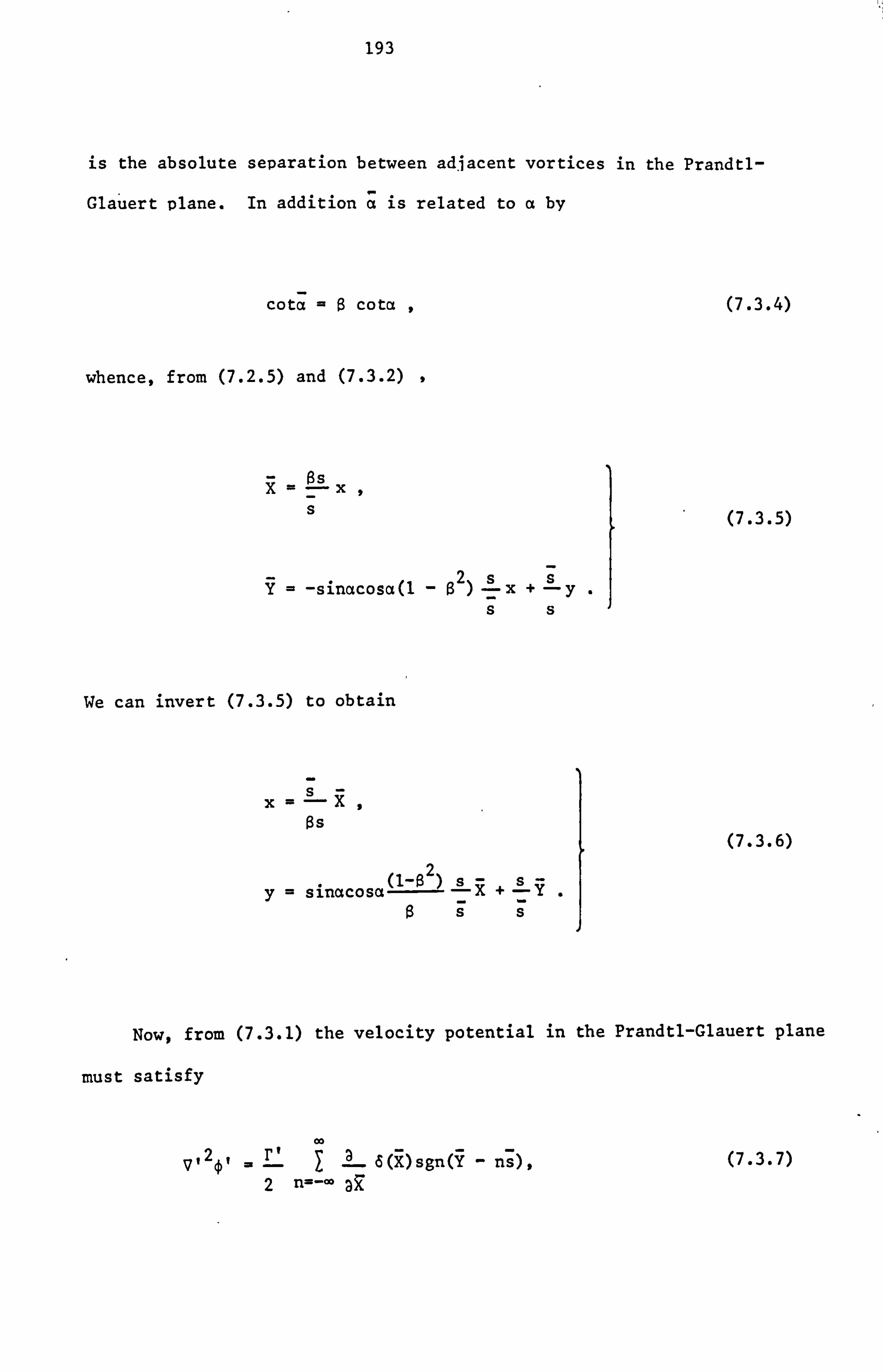
193

is the absolute separation between adjacent vortices in the Prandtl-

Glauert plane. In addition ä is related to a by

cota =B cots!

whence, from (7.2.5) and (7.3.2) ,

as x

s

Y -sinacosa(1 - ß2) s x+ s

y. ss

We can invert (7.3.5) to obtain

X=s as

2 y= sinacosa(l-ß

3X+ s_ Y. ßss

(7.3.4)

(7.3.5)

(7.3.6)

Now, from (7.3.1) the velocity potential in the Prandtl-Glauert plane

must satisfy

p, 2e,

3 rt ia d(X)sgn(Y - ns), (7.3.7) 2 n='°° 3

194

where r' is the circulation about each vortex in the new system.

(7.3.5) and (7.3.6) we can rewrite (7.3.7) as

r (1-ß )sa V12ý = rl 7 Is a+ 2

_. sinacosa

2 n=-ý ßs 8x ßs ay

ö ßS x sgn -sinacosa(1-ß2) !

_x +S (y-ns) ,

ss

which reduces to

co V'24' =r2I C(sin2a+ß2cos2a)d'(x)sgn(y-ns)

2ß n=-()o

+ 2sinacosa(1-0 2)6(x)6(y-ns)]

From

(7.3.8)

(7.3.9)

In appendix 7.2 it is shown, from Poisson's summation formula, that

sgn(y-ns) =i exp(-i2nny/s)

n=-ý n n=-ý n (7.3.10)

By writing the series of delta functions in y in Fourier series form, as

in section 7.2, we then obtain

195

'2ý' = ir, 00 [sin2a+2cos2)(x) -$ i2ýn sinacosa(1-ß2)

n= ý d(x)]

2nß -

exp(-i21rny/s)

n

(7.3.11)

Following the procedure used in section 7.2.1 we then find that ý is

given by

ý= it

sgn(x) 1ExEy

(7.3.12) 41r n=-00 n

where EX and Ey are defined in (7.2.18) and (7.2.19) respectively. The

circulation r in (7.3.12) is related to the 'incompressible' circulation

r' by

r=r ß

(7.3.13)

as shown, for example, by Landau & Lifshitz (1959) and Ward (1955).


We now consider an airfoil upstream of the cascade: the situation

is shown in Figure 6.2. By following the analysis in sections 6.2.2 and

7.2.2 we find that the upwash can be written in the same form as (7.2.21)

with (7.2.22) replaced by

196

rrB2 vl = (cosal - in sina1)

4 Irr 2

(7.3.14)

exp2B2 Gn2(g - cl

Cosa l) +i cl

sinal] r22


Here we consider an airfoil dgwnstream of the cascade as shown in

Figure 5.1. The analysis used in sections 5.4.1,6.2.3 and 7.2.3 is

applicable. We find that (7.2.27) is again appropriate to describe the

upwash, with the gust amplitude v2 replaced by

rl3 l v2 (cosa2 + inisina2) 4 Trr

(7.3.15) IX181

In1(g - C2

cosa2) -i C2

exp sina2] r22

7.4 Response of the Upstream Row

As we mentioned in chapter 5, the response of an airfoil to a gust

in compressible flow has, in general, to be calculated numerically.

However, in the case of high frequency interactions, an approximate solution

can be obtained by considering the airfoil to be semi-infinite and solving

197

only the trailing edge problem. This is similar to the problem discussed

in chapter 5 except that, in this case, the gust is not convected with

the mean flow. In addition, since we are considering a trailing edge, the

inverse square root singularity at the edge will be removed by imposing

a Kutta condition.

in chapter 6, where'the incompressible flow case was considered, we

found that the semi-infinite airfoil approximation can lead to errors

due to the neglect of important leading edge effects. We will therefore

apply a correction to the semi-infinite airfoil solution which accounts

for the leading edge effects. This correction will be discussed in the

following section.

In the (X1, YI) coordinate system fixed to the forward blade row

(see Figure 6.2) the velocity potential satisfies the convected wave

equation

2

p2ý - 12 a+

Ur a=0 (7.4.1)

co at 1 8X1

Since 4 has a time dependence e iü

it (7.4.1) reduces to

(1- M2) as

+a? L

-2ikM r 30

+k2ý=0 (7.4.2) r1 ax1

2 ayl 1 axl

where

198

k=1, (7.4.3) c 0

U

Mr = rl

. (7.4.4) 1c

0

The upwash is given by (7.2.21). On imposing a hard wall boundary

condition we obtain

Yxlx1+iwlt

+ vle 8Y1

= 0; X1 < 0. Y1 = 0. (7.4.5)

We now define a new velocity potential ýP, and a new set of coordinates

x and y, where

iv +iu t

e(Xl. Y1) = (D (X, Y)e (7.4.6)

X° Xlf

(7.4.7)

Y= KY1,

and v and K are to be determined. On substituting (7.4.6) and (7.4.7)

into (7.4.2) we obtain

199

22 (1 - M2 )8_ý + K2

a_ý + G2iv(1 - M2 )- 2ikM ä aý

r1 äX2 3y2 r r1 ax

+ Ck2 + 2vkM - v2 (1 - M2 ) ]0 =0. r1 r1

If in (7.4.8) we set

K= (1 -M2 1

kM rl

v2 (1-M )

rl

then (7.4.8) reduces to the Helmholtz equation

22 20 +

!a+K=0 22

ax ay

where

K= (1

k

- Mr) 1

(7.4.8)

(7.4.9)

(7.4.10)

(7.4.11)

The normal velocity on the blade surface is

200

2 8(P ivx+iwl

_ (1 M )`- e 8Y1 r1 8y

If we now define another velocity potential ý by

(1 - Mr )

r

then the boundary condition, (7.4.6), reduces to

v*x

ay X<0, y=0 .

(7.4.12)

(7.4.13)

(7.4.14)

In (7.4.14) v* is defined as

v* =y iv . 1

The pressure is given by

p -pes- +U !

- 8t r1 ax

(7.4.15)

(7.4.16)

where p is the density. From (7.4.6) and (7.4.13) we can rewrite this

in terms of j as

201

-pvIUr

eivx+iwIt p, (7.4.17) (1 -Ir )

1

where

p* = ik*ý + aL (7.4.18)

aX

and

k k* _ (7.4.19)

M (1, -M ) r1 r1

We now look for the solution to

72* +K2ý=0 (7.4.20)

with the boundary condition (7.4.14).

The solution is obtained by the Wiener Hopf technique and will be

described here in detail. We define 0 and G Fourier transforms by

T+(s. Y) s «Xj) H(± )eisx dx (7.4.21)

where H(x) is the Heaviside unit function. The inverse transform is

given by

202

ý(X, y) =1

21r .

-isx T(s, y)e ds (7.4.22)

On Fourier transforming the Helmholtz equation, (7.4.20), we obtain

W11 2

I (s, y) + xi'(s, )=0f (7.4.23)

where we use primes to denote differentiation with respect to y and

(Ký-s2)

Here we choose the branch of the square root so that

X -i! sl as s-±-.

(7.4.24)

(7.4.25)

The branch cuts in the complex plane are shown in Figure 7.2. The wave-

number K is taken to have a small imaginary part.

We now consider the region x>0 where we assume continuity of pressure

across the wake. From (7.4.17) p* is also continuous across the wake so

that, on Fourier transforming (7.4.18), we obtain

i(k* - s)[T+(s, 0-) -T +(s, 0+)] =0,

203

Since ý must be an odd function of y this leads to

+(s, 0+) = 0. (7.4.26)

If we now take the Fourier transform of p* in the region x<0 we obtain

-2i(k* - s) '_(s, O+) = eP*(s) (7.4.27)

where we have again used the fact that ý is odd in y and 1P* represents

the transform of the jump in p* across the airfoil.

The boundary condition, (7.4.14), can be Fourier transformed to

give

ß'(s, 0) e V*X+1SX

dx

-co

1.

(S - 1V*)

where the integral converges provided that

Im(s) < Re(v*) .

(7.4.28)

(7.4.29)

From (7.4.23) and the requirement that the fields decay at infinity

we obtain

204

T(s, y) = C(s)e'-"XY (7.4.30)

where we have taken 7 to be positive. (For y negative we can again use

the fact that ý is odd in y. ) On differentiating (7.4.30) and setting

0+ we obtain

ß'(s, 0) = -iX'(s, Of) . (7.4.31)

On substituting (7.4.26) and (7.4.28) into (7.4.31) we find that

`Y+(s, O) +i= --iX'Y-(s, 0+) " (7.4.32) (s - iv*)

We now write X in the form

X (K + s) ' (K - s)

' (7.4.33)

so that, on dividing through by (K - s)1, (7.4.32) becomes

''(s, 0)

(K -. s) +

(s - iv*)(K - s) =- i(K + s)'Y_(s, O+) . (7.4.34)

Here the first term on the left hand side is a 1+ function and the right

hand side is a (D function. We can rewrite the second tern on the left hand

205

side as

1

(s - iv*) (K - iv*) +

i1_1

(s - iv*) (K -

s) (K -

iv*)'ý (7.4.35)

where the first term is G function (since, from (7.2.35) and (7.4.15),

iv* lies in the upper half plane) and the second term is a (D function.

We thus rewrite (7.4.34) as

+(s'o) +

(K - s)l (s - iv*) (K -s (K - iv*)

-i(K + s)''_(s, O+) _i (s - iv*) (K - iv*)

(7.4.36)

where the left hand side is a(@ function and the right hand side is a

G function. By the usual arguments resulting from Liouville's theorem,

both sides of (7.4.36) are equal to an entire function E(s) which must

be identically equal to zero (otherwise '+(s, 0) would diverge as s

implying that 4 has a singularity at the origin). From (7.4.27) and the

right hand side of (7.4.36) we then obtain

AP* (s) = 2i (k* - (7.4.37) (K - iv*)'(K + s) (s - iv*)

206

We now apply the inverse Fourier transform, as defined by (7.4.22),

whence

OP* (X) =1

ir(K - iv*)

(k* - s)e-isx ds (K + s) (s - iv*)

(7.4.38)

On wrapping the integration contour around the branch cut in the upper

half plane we obtain

a

2eIK +i, rf4 Ap*(X)

n(K - iv*) J 0

(k* +K- is')exs ds'

s' (s' + iK - v*)

- 2(k* - iv*)

exv* (K2 + v*2)

(7.4.39)

where the final term represents the contribution from the pole at s- iv*.

Alternatively,

2e1Kx-iir/4 tp*(x) =_i CI1 + (v* + ik*)I2]

-ff (K - iv*)

k* - iv*) ' xv* -e

(K2 + v*2)

(7.4.40)

where

207

J XSt 3

I1 =e ds' _ s'i Ix'I i

0

and, from Abramowitz & Stegun (1965),

(7.4.41)

Xs'

I_e ds'

_ (i K-

v*)'] (7.4.42) 2J s' (s' + iK - v*) K- v*)

0

where we have used x=- ýxý since x is negative on the airfoil. 'Then,

combining (7.4.40) to (7.4.42), we obtain

Qp*(X) = -2 (K 2(

+ v*

v* +2ik*) e1Kx w[ijxjl(iK - v*)'I-ev*X

)

2eiKx-iir/4 + it (K - iv*) IXI

(7.4.43)

We now impose a Kutta condition at the trailing edge of the airfoil. In

appendix 7.3 we show that this is equivalent to removing the inverse

square root singularity at the trailing edge. Then, from (7.4.17) and

(7.4.15), the pressure jump across the airfoil is given by

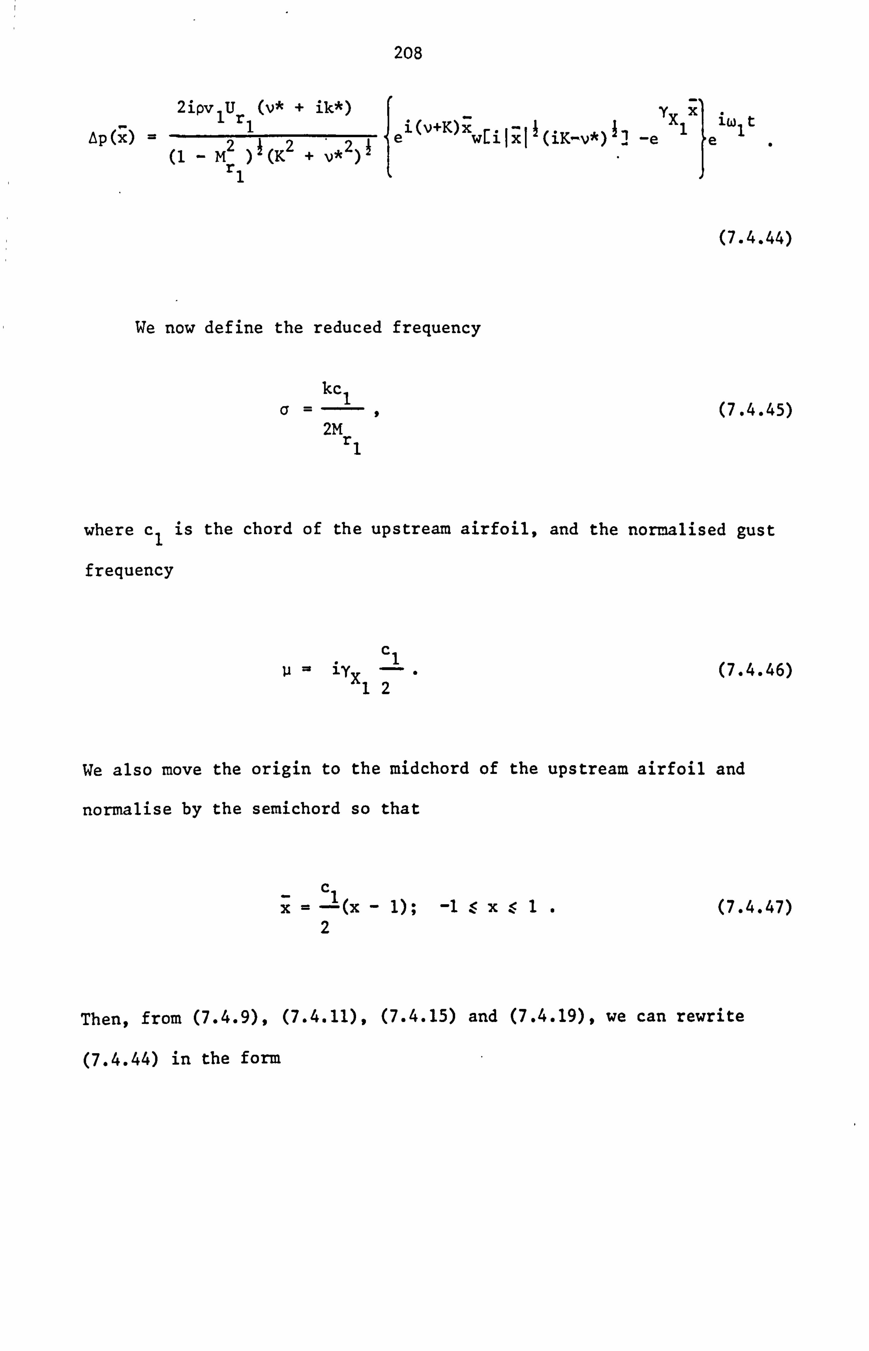
208

2ipv1Ur (v* + ik*) YX X iw t Ap(x) =2

11 22 el(v+K)xwlijxj1(iK-v*)'1- -e e1

(1 - Mr) (K + v* ) 1

We now define the reduced frequency

kcI Q=,

2M rl

(7.4.44)

(7.4.45)

where c1 is the chord of the upstream airfoil, and the normalised gust

frequency

C1 u iyx -.

12 (7.4.46)

We also move the origin to the midchord of the upstream airfoil and

normalise by the semichord so that

_C X= -(x - 1); -1 :x$1.

2 (7.4.47)

Then, from (7.4.9), (7.4.11), (7.4.15) and (7.4.19), we can rewrite

(7.4.44) in the form

209

ap

-2ipv1Ur1(Q - u) () =2_ elý*(x-1)wE. (1-x)l(iu+iQ*) 7

(1 - Mr) (ia* + iv) (iQ - iu) 1

elw1t

where we have defined

QM

and

rl Q* _

(1-Mr) 1

QM r1

Cy = (1+Mr)

1

(7.4.48)

(7.4.49)

(7.4.50)

The total lift on the airfoil is obtained by integrating (7.4.48)

along the airfoil chord (and multiplying by the semichord). We also need -ik x

to include the phase term ex which was introduced in chapter 4 and

represents the noncompactness effects. The 'effective' unsteady lift

per unit span, i. e. the point force which generates the same far-field

sound (the actual unsteady lift per unit span is obtained by setting the

chordwise wavenumber kX equal to zero), is then given by

210

dL 1 pvIUr

1 c1(a - u)e

iwl t-ikX

dr (1 - M2 )1(u + kX) (iu + iQ*)' (icr ý- iu) l

1

-iTr/4 (iv + ia* -i2(Q*-k X) e1-e w(-(1 k) l (Q* - kX X )

i2(u+k ) -i2(a*-k -e

x+ wEi2l(iii + iQ*)lle x

(7.4.51)

If in (7.4.48) and (7.4.51) we let Mr }0 (the reduced frequency is, 1

in this case, written as a= wlc1/2Ur which is the incompressible flow

limit, then we obtain the results (6.4.4) and (6.4.5)*. This serves as

a partial check on the results of this section.

In the current section we have dealt with just the trailing edge

problem and consequently any leading edge effects have been neglected.

Since, in chapter 6, we showed that leading edge effects can be important

we will discuss a correction to the present results to account for these

effects. This discussion forms the basis for the next section.

7.5 Leading Edge Correction

We will use a technique developed by Landahl (1961) and Adamczyk (1974),

and discussed by Anriet (1973,1975), for downstream convected gust

FOOTNOTE

* Note that particular care must be taken with the low argument limit of the first w-function in (7.4.50) as a* ;0 in order to remove the inverse square root singularity (a*-kx)-I with kX a 0.

211

interactions. This involves an iterative technique for the solution of

a three part boundary value problem. The situation is shown in Figure

7.3 with the upwash specified on -cl x<0. The first iteration

involves solving the trailing edge problem with the upwash specified on

<x<0; this is the case discussed in the previous section. The

second iteration involves correcting the upstream boundary condition on

-ý <x<- cl without affecting the boundary condition on the airfoil, i. e.

on -cl. x<0. We therefore require the "new" pressure difference across

-CO <x cl to be minus the pressure difference obtained on the first

iteration, and the upwash on -cl <, *; <- to be zero. This second

iteration induces an error in the boundary condition on 0<x<- which

could be corrected by a third iteration and so on. (In fact, we are

likely to obtain a finite, but non zero, pressure jump at x-0 corres-

ponding to the airfoil trailing edge. )

We define a new coordinate x centred on the airfoil leading edge so

that

XaX+ cl. (7.5.1)

The pressure jump ßp2 across -ý <x<0 is minus that obtained in the

previous section so that

Op2(x) = -AP(X) - -Lp(x - c1). (7.5.2)

Then, from (7.4.17) and (7.4.18),

-ivc1 Op2(x) = -e Op*(x - cl)

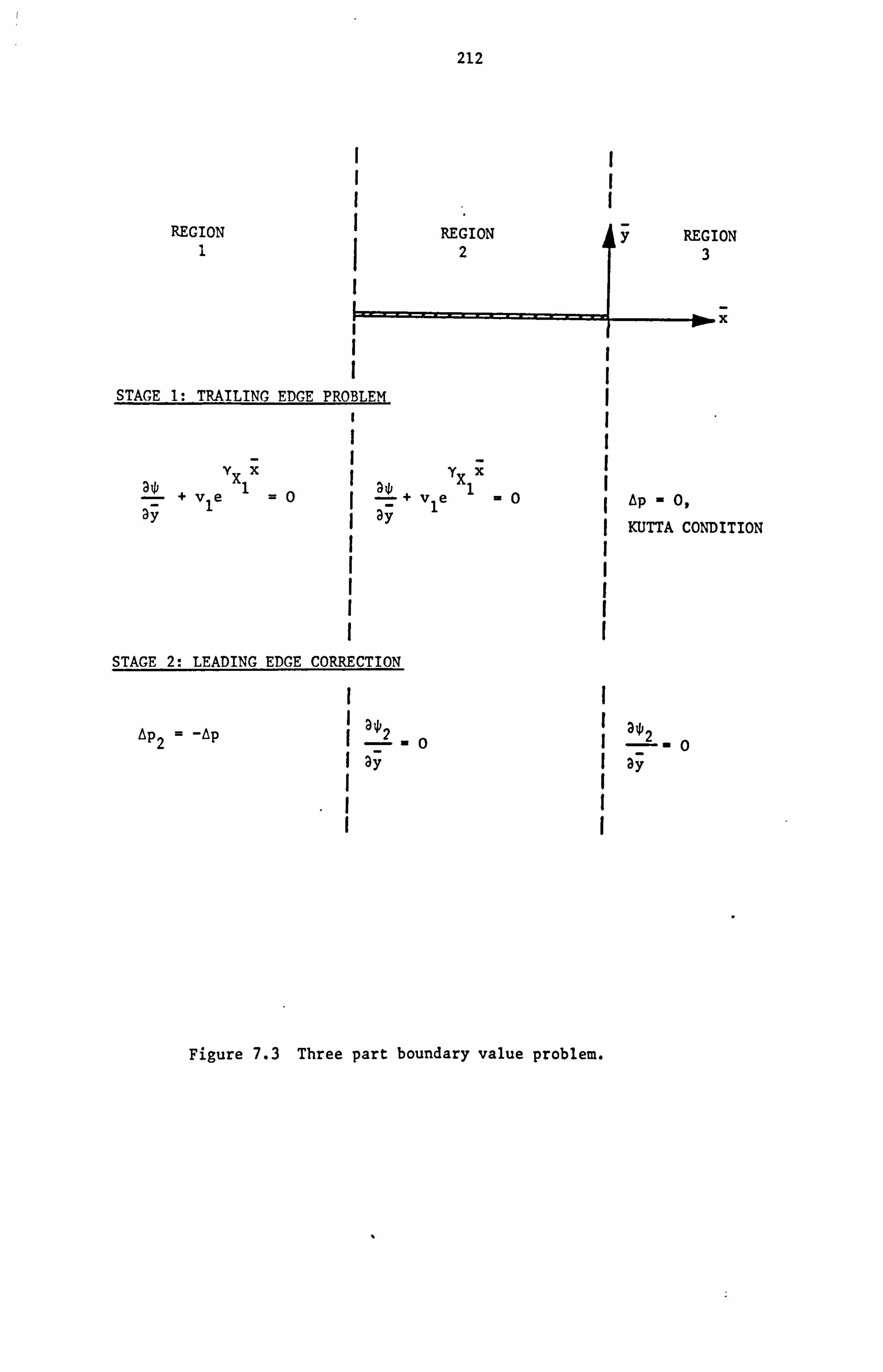
212

REGION I

REGION y REGION 1I23

X

I II

STAGE 1: TRAILING EDGE PROBLEM

YX L+

v1eYX1X =O1 a-

+ °1e X1

O( AP - 0, ay ý ay ý KUTTA CONDITION

j

STAGE 2: LEADING EDGE CORRECTION

I 3ý aý 6p2 = -gyp ?-0I2-0

ay I ay

.1I i

Figure 7.3 Three part boundary value problem.

213

(We will use the suffix 2 throughout this section to denote "second

iteration" values. ) From (7.4.43) we then obtain

2i(v* + ik*) -ivcl iK(x-c1) v(x-cl) Ap*(x) =22ee w[iJx-cl1 (iK-v*) I_e

(K + v* )

(7.5.3)

(recall, from the discussion following (7.4.43), that the inverse square

root singularity term has been removed in order to satisfy the Kutta

condition). Since we are considering a high frequency problem kc1 and

'1 c1 are both large. Then, from (7.4.9), (7.4.11) and (7.4.15), the

argument of the w function in (7.5.3) is also large on x<0 so that,

from Abramowitz & Stegun (1965),. we can use the approximation

w[ilx - c, lý(iK - v*)'] ti Tr ]x - clj UK - v*)

(7.5.4)

(In order to use this approximation we have used the fact that

jarg(iK - v*)'] < 7/2. ) In addition, since yX cl is large, the last

term in (7.5.3) is, from (7.4.15), exponentially small on x<0.

Consequently, this term will be neglected. The jump in p2 across x<0

can therefore be approximated by

214

-ivc1+iK(x-c1)

Ap2(x) ti 2i(v* + ik*)2-

2 7 (iK - v*) (K + v* )x- cl

The boundary condition is that of no upwash so that

alp 2 ---=0 x>0 . (7.5.6) ay

In (7.5.6) we have, for consistency, replaced y with y.

The problem is therefore defined by the Helmholtz equation, (7.4.20),

with the boundary condition (7.5.6) and the jump in p2 across x<0 given

by (7.5.5). The solution is again obtained by the Wiener-Hopf technique

with G+ and G Fourier transforms defined by (7.4.1) and the inverse

transform defined by (7.4.22).

The Fourier transform of Lp2(x) is given by

dP* (s) 2i(v* + ik*)e-ivcl-iKc1 0

ei(s+K)x dx . (7.5.7) 2

7r(iK - v*) (K2 + v*2 (c-X)

We now use the fact that Kc1 is large. On normalising x in (7.5.7) by

cl we find that the integrand oscillates rapidly. Then the integral is

dominated by contributions from near x-0 and, by following Murray (1974),

we can approximate (7.5.7), to leading order in I, by c1(K+s)

215

Ap* (s) - *) e

-i(v+K) cl (7.5.8)

_ 2(v* + ik

2- ýr c1 (iK -- v*) (K2 + v*2)

i (s + K)

From this point we proceed with the Wiener-Hopf technique in the

usual manner and the pressure jump Op2(x) is finally obtained as

Ap (x) =

iPv1Ur 1

(a - u)eiw 1 t+iQ (1-x)-4jQ

2'

2 ir1 (1 - Mr ) (iu+iQ*) (iQ - iu)

1 (7.5.9)

-iTr/4- 1 21e-in/4 wC-2 ev (1 + x) ]-

7r fQIti (1 + x)

#

where we have reintroduced the normalised frequencies a, V, a* and a given

by (7.4.45), (7.4.46), (7.4.49) and (7.4.50) and, in addition, we define

M _

r. Q=2a. (7.5.10)

1 -H rl

(1 +M)

all = rl

a. (7.5.11) M (1 -M) r1 r1

We note, from (7.5.9), that we have restored the inverse square root

singularity at the airfoil leading edge (recall that the pressure distrib-

216

ution on the airfoil is now given by the sum of (7.4.48) and (7.5.9)).

Comparing (7.4.48) and (7.5.9) we see that, apart from the exponential

decay term e- lux in p and the inverse square root singularity (1 + x)-

in p2, the first and second stage solutions are basically of the same

form apart from the factor (iv + is*)-l in p2. Since we are considering

a high frequency problem both u and a (and hence a*) are large!. This

suggests that, in the high frequency limit, the first correction to the

trailing edge problem is 0(Q-1) smaller than the leading order term.

The total lift, per unit span, on the airfoil is obtained by

integrating (7.5.9) along the airfoil chord (and multiplying by the

semichord). As in the previous section we will include the phase term -ik x

ex which was introduced in chapter 4 and represents noncompactness

effects. After some manipulation we obtain

dLl -pv1Ur c (c - p) e iw1 t+ik Xi2Q*

21

dr =

21ni(1 - M2 )1(iu + io*)(ia - iu) 1

-i2(a+k ) 1- w(-2e-iý/4Q )e x (7.5.12)

(a - kX )

I- w(-2 e ii/4(a +k )e-i2(Q+kX) 1_Q

x +2

xall (a*-kii

The total "effective" lift (i. e. the magnitude of the lift that determines

the amplitude of the far-field sound) is then given by the sum of (7.4.50)

217

and (7.5.12). Note that, as we suggested in the last paragraph, the

first correction to the trailing edge problem is O(a "I) smaller than

the leading order term - even when the inverse square root singularity

at the airfoil leading edge is included. We conclude that, in the

high frequency limit, the semi-infinite airfoil model is a valid

approximation and provides accurate results to leading order in a.

Recall that, as we found in chapter 6, the same conclusion does not

hold in the incompressible flow case where the semi-infinite airfoil

approximation leads to errors in the unsteady pressure, away from the

trailing edge, which affect the final result for the total fluctuating

lift, per unit span, acting across the airfoil.

7.6 Response of the Downstream Row

In the previous two sections we considered the interaction of the

potential field, generated by the downstream blade row, with the upstream

airfoils. We now consider the interaction of the potential field,

generated by the upstream blade row, with the downstream airfoils. As

in section 7.4 we consider the high frequency limit and model the airfoil

as a semi-infinite flat plate extending to downstream infinity. The

Kutta condition is inappropriate here since there is no trailing edge.

We could, of course, follow the procedure discussed in the previous

section for a three part boundary value problem and add a correction to the

leading edge response so that the final solution satisfies the trailing

edge Kutta condition. However, the airfoil response is likely to be

dominated by the leading edge inverse square root singularity so that the

trailing edge region should be relatively unimportant. Moreover, as we

showed in section 7.5, the correction terms are 0(c^1) smaller than those

resulting from the semi-infinite airfoil approximation. We will therefore

218

consider just the leading edge problem.

On following the analysis at the start of section 7.4 we can

reduce the problem to that of finding a potential *(x, y) which satisfies

the Helmholtz equation

where

v 2iy+K. 2ý=0, (7.6.1)

K=k r (7.6.2)

(1 -M ) 2

and k= w2/co with w2 defined by (6.2.25), with the boundary condition

3ý -

ay

The coordinates x and y are given by

and

x2

y=(i-M2 r2 Z,

(7.6.3)

(7.6.4)

where X2 and Y2 are shown in Figure 5.1, and in (7.6.3) the wavenumber v*

is given by

219

v* = YX - iv 2

where

kM r 2

v= (1- .

Mr) 2

We write the pressure in the form

-ov2Ur2 iw2t+ivx p

(1 - MTA e

2

where

p* = ik*l + 31ý

3x and

k k* =

m (1 - M ) r r 2 2

(7.6.5)

(7.6.6)

(7.6.7)

4

(7.6.8)

(7.6.9)

The solution is again obtained by the Wiener-Hopf technique whence

ep*(X) = 2(v* + ik*)

(iK - v*) (iK v*) e-iKx wEix (iK + v*)']-exv*

_ 2e iKx

7rß (iK - v*) x1

(7.6.10)

where all the complex wavenumber square roots are now defined with a

220

branch cut along the negative real axis. The pressure jump Ap is then

found from (7.6.7) and (7.6.10). If we introduce the reduced frequency

kc2 6=ý

2M r2

(7.6.11)

where c2 is the chord of the downstream airfoil section, the normalised

gust frequency

c u= iyX 2 (7.6.12)

22

and a normalised coordinate x, which is related to x by

c x=? (x + 1), (7.6.13)

2

then the pressure jump can be written in the form

AP(x) a

-2pv2Ur 2e

iw2t

(1 - M2 + r2

Le iQ(x+l

(-ii, iQ)

b(i(x + 1) (-iv + iQ))-e

iu(x+1) (7.6.14)

+

-iQ (x+1)

7r 1 (x + 1)

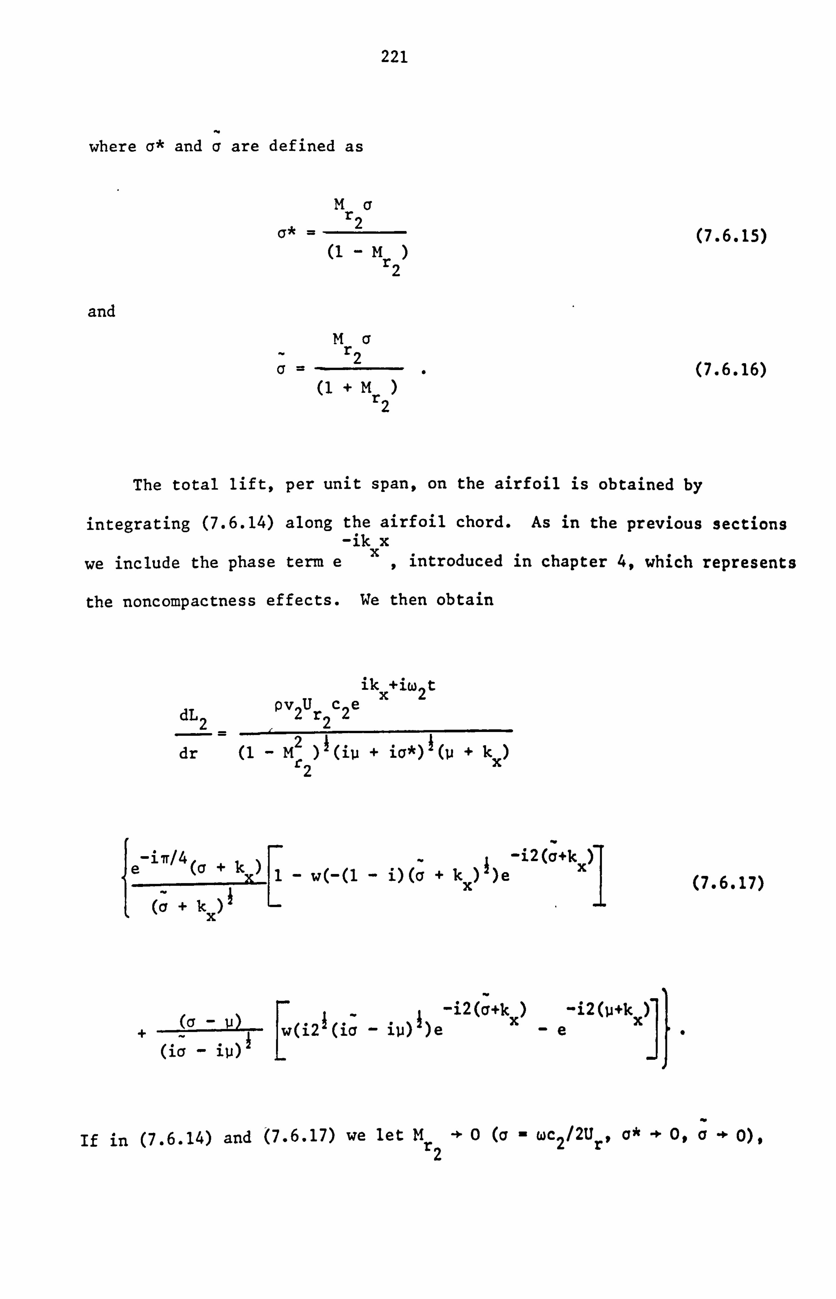
221

where a* and a are defined as

MQ r2

Q* _ (7.6.15) (1-M

2

and MQ

Q= ~ r2

(7.6.16) (1 +Mr )

2

The total lift, per unit span, on the airfoil is obtained by

integrating (7.6.14) along the airfoil chord. As in the previous sections -ik x

we include the phase term ex, introduced in chapter 4, which represents

the noncompactness effects. We then obtain

ik+iw2t

dL 2 pv2Ur

2 c2e

dr (1 - M2) (ill + is*)l(U + kX) 2

{14 (Q + kX) 1- w(-(1 - i)(Q +k )e-i2(Q+k x)

x (7.6.17) (o + kx

+ (Q - u)

[w(i2(i;

- iu) )e-i2(Q+kX) -e

i2(u+kX)

" (iQ - iU)

If in (7.6.14) and (7.6.17) we let Mr 2}0

(a - Wc2/2Ur, a* - 0, a 0),

222

which is the incompressible flow limit, we regain the results (6.5.4)

and (6.5.5).

7.7 Low Frequency Response

The response calculations in the three previous sections have been

specifically aimed at the high frequency limit since, in general, this

is the regime which is most appropriate to the interactions on high

blade number counter-rotation propellers. However, there are occasions

on which interactions take place at low reduced frequencies (some of

these will be discussed in the following section). It is therefore

necessary to consider low frequency interactions. In the case of

convected gust interactions, i. e. wake interactions, which were discussed

in chapter 5, we only considered the high frequency limit. Our reasons

for discussing low frequency potential field interactions and not low

frequency wake interactions is that, as became clear in chapter 6, the

potential field interactions are much more significant than wake inter-

actions at low frequencies*.

The response of an airfoil to a nonconvected gust in compressible

flow, in the low frequency limit, has already been provided by Osborne

(1973) and Kemp (1973) who followed on from the basic theory of Amiet

& Sears (1970). However, their approach, and notation, was somewhat

different from ours. Furthermore, we require not the total airfoil lift

but the effective lift when acoustic noncompactness effects are taken into

account. In addition, for the sake of completeness, we wish to relate the

FOOTNOTE

* This conclusion has been obtained just by consideration of the data from the Fairey Gannet flyover tests. Since there are major differences between Gannet propeller blades and advanced propeller blades the same conclusion does not necessarily apply to the propfan.

223

compressible flow results to the incompressible flow results which were

given in chapter 6. We shall therefore solve the problem in detail.

our starting point is the boundary value problem described by

(7.4.14) to (7.4.20). (We note, in passing, that the coordinate trans-

formation given by (7.4.6), (7.4.7) and (7.4.9), which reduces the wave

equation to a Helmholtz equation, is equivalent to the combined Galilean-

Lorentz transformation used by Anriet & Sears (1970) and Osborne (1973)).

In order to apply the results to both upstream and downstream interactions

we introduce the upwash

w(x t) =w0 eiwt-ijix (7.7.1)

where p and x are defined by (7.4.46) and (7.4.47) for upstream inter-

actions and by (7.6.12) and (7.6.13) for downstream interactions. The

coordinate x is centred on the midchord in both cases. The upwash

amplitudes v1 and v2 in (7.4.17) and (7.6.7) respectively can then be

replaced by relating them to 0 as appropriate. We scale all lengths

on the semichord. We then require the solution to

v20' + Ký20, _0 (7.7.2)


air = -e-iufX

a on -1 Sxg1 (7.7.3) y

where

224

and

QM KI =r

(1 Mr)

QM2 r + (1 - Mr)

The pressure jump across y=0 is given by

-pw U iLM2x

r

Apr Ap =° 2r A exp r2+ iwt (1 - M) ` (1 - M2)'

r)

where

Ap _ iQ'4' +W aX

a

v- ý1 - Mr)

(7.7.4)

(7.7.5)

(7.7.6)

(7.7.7)

(7.7.8)

Since we are considering the low frequency limit we assume that K' is

2 small and neglect K' . The Helmholtz equation (7.7.2) then reduces to

Laplace's equation. The problem is then completely analogous to that

considered by Kemp (1952) in the case of incompressible flow. The

pressure distribution across the airfoil for this case is given by

Amiet (1973) and was described in chapter 6. We then obtain

225

Apt _ -2 1-

xx IcýQý)(Jo(u`) - iJliuý)) + 1J1(u`)7

1+

(7.7.9)

-11- a' (1 - x2)1I' Tr u,

where I' is the singular integral

_e I (x - ý)(1 - ý2)

dg . (7.7.10)

-1

We see, from (7.7.6) and (7.7.9), that the total lift acting on the airfoil

section is not the same as that given by Kemp (1952) (with the transformed

temporal and spatial reduced frequencies, a' and u') because of the phase

factor exp[iaMr2 x/(1-M2)] in (7.7.6). In addition we need to include the

noncompactness phase factor exp(-ikxx) in order to obtain the "effective"

lift (or dipole strength) as observed in the far acoustic field. (Since

we are considering the low frequency limit the noncompactness effects are

likely to be small. However, for the sake of consistency, we retain all

first order wavenumber terms. ) The chordwise integrations, including these

phase terms, are carried out in appendix 7.4 where it is shown that the

"effective" unsteady lift, per unit span, acting across the airfoil is

given by

226

dL pw Urcitelwt o-

{EJ

(u') - iJ1(u') ]Cc (Q') (J (n') - iJ1(n t)) + iJ(n t) ] dr (1 -M2)001 r

(7.7.11)

i(Q+k ) +

(uý _x

CJo(n')Jl(u') - J1(n')Jo(u')]

where

M2a r1 =r

(1 -M 22- kX . (7.7.12)

) r

If, as in the three previous sections, we let Mr tend to zero we find

that the compressible flow result (7.7.11) tends to the incompressible

flow result given by (6.6.9)

The above analysis should be accurate to 0(K'). However, Miles

(1950a, 1950b) has questioned the validity of the 0(K') approximation

when an infinite wake is present. Problems arise when logarithmic terms

such as Rn(K') appear in the solution. By direct expansion of the exact

Poissio integral equation, Miles derives results for a«1 and Mr«1.

Amiet (1974) showed that in the case of a convected sinusoidal gust, the

Miles solution differed from the Osborne (1973) solution by an O(kM2)

phase term. One piece of further work, therefore, would be to update the

results of this section by calculating the Miles/Anriet correction for a

nonconvected gust.

In the following section we proceed to make comparisons between

counter-rotation propeller noise interaction tones, as calculated using

the results for airfoil response from this chapter, and measured data.

227


In the previous sections of this chapter we have calculated the

unsteady lift* generated on both upstream and downstream blade rows

due to the interaction of the blades on each row with the bound potential

field of the adjacent blade row. We showed, in chapter 4', how the

far-field acoustic pressure could be calculated once the unsteady lift

is known. In this section we will compare the Gannet flyover measure-

ments with the predicted acoustic field using the results from both the

current chapter and chapter 4. We shall also refer back to the comparisons

between measurements and predictions which were shown in chapter 5, where

just the downstream wake interaction was considered, and chapter 6, where

the potential field interactions were considered but the flow was assumed

to be incompressible.

We start with the high frequency response calculations given in

sections 7.4 to 7.6. Since the validity of the Kutta condition in

unsteady flow is a matter of controversy at the moment (see the

discussion in appendix 7.3) we calculate the response of the upstream

blades to the potential field of the downstream blades both with and

without the Kutta condition imposed. (As we show in appendix 7.3, this

corresponds to rejecting or retaining the inverse square root term in

(7.4.43). )

The first interaction tone generated by the Gannet is the (1,1)

FOOTNOTES

* As we pointed out during the analysis, we have in fact calculated the effective (chordwise) point loading that gives the same far-field

acoustic pressure as the (chordwise) distributed loading when interference effects are taken into accout.

t See also Hanson (1985a).

228

interaction. The far-field directivity of this tone is shown in

Figure 7.4. The predicted far-field noise, due to the upstream and

downstream potential field interactions with a Kutta condition imposed

at the trailing edge of the upstream blades, is typically 5dB higher

in the forward arc (0 <0< 90°), and up to 10dB higher in the rear

arc (90° ;0; 180°), than was calculated in the incompressible flow case

(see Figure 6.5) and compares extremely well with the measured data.

(Since the upstream and downstream potential field interactions are

spatially separated the phase relationship between the two sources is

not just that given in the current chapter but must be corrected in the

manner described by Hanson (1985a). For the present we consider the

sources separately. ) The next two interaction tones generated by the

Gannet are the (2,1) and (1,2) interactions for which directivity plots

are shown in Figures 7.5 and 7.6. Here, as for the (1,1) interaction,

the predicted noise levels are between 5dB and 10dB higher than was

calculated in the incompressible flow case (see Figures 6.6 and 6.7) and

agree well with the measurements, although there is a small discrepancy

in the rear arc for the (1,2) interaction.

In Figures 7.4 to 7.6 we have also plotted the predicted far-field

noise due to the upstream potential field interaction* using the high

frequency response calculation with no Kutta condition imposed at the

trailing edges of the blades. In this case the predictions are,

typically, 5 to 10dB higher than the predictions for which a Kutta

condition was imposed at the trailing edges. In addition there appears

FOOTNOTE

* i. e. the interaction of the upstream blades with the potential field

generated by the downstream blade row.

229

IOdB

IO

FWD. POT. (NO KUTTA COND. )

'% "ý MR

11T

: ". I

WAKE I

7-

Gü0 ANGLE

Figure 7.4 Gannet measurements vs predictions for the (1,1) interaction tone. The potential field predictions are obtained using semi-infinite airfoil response calculations in compressible flow.

Fwr)L TNK TA N.

MEASURED

.r"f .ý :\ FWD. POT.

:"0 RWD- POT.

/. I`. it b R\ %I

WA K

/, /ýý

/

Fwa POT.

%% . 'j

iý

ANGLE

ao /AO 80.0 120,0 160-0


tone. The potential field predictions are obtained using semi-infinite airfoil response calculations in compressible flow.

230

FWD POT (NO KUTTA COND. )

lOdB \ MEASURED RWD POT

i: %% FWD POT ýf

ýý, ýý

"'ý ^` ý.

% \ `ff

1ý 11f

"t1 /f

1 ý,

1 ff

N 1. ý f WAKE IFS Ir " 'r .

.r

0.0 4 .0A. 0

4.0 16 .0

ANGLE

Figure 7.6 Gannet measurements vs predictions for the (1,2) interaction tone. The potential field predictions are obtained using semi-infinite airfoil response calculations in compressible flow.

lOdB

T I/ 'I `` \ /

/1\+

-.

ANGLE

80.0 120.0 160.0


tone. The potential field predictions are obtained using low frequency

airfoil response calculations in compressible flow.

0.0 40.0

231

to be some change in directivity, particularly for the (1,1) interaction

where the forward arc levels are raised and the rear arc levels are

lowered when no Kutta condition is imposed. These results seem to

agree qualitatively with those of Howe (1976), who found that the

application of a Kutta condition reduces the level of acoustic radiation,

and Rienstra (1981), who found that the sound field diffracted by an

airfoil has directivity properties which are strongly dependent on the

trailing edge condition. The results presented here seem to indicate

that it is appropriate to apply the trailing edge Kutta condition for

the interaction frequencies we have considered on the Gannet. This

follows the suggestion of Crighton (1981) that far-field acoustic

measurements, along with theory, may be the optimum way of determining

the correct trailing edge condition.

The high frequency response calculations, with a Kutta condition

imposed at the trailing edge of the upstream blades, agree extremely well

with far-field acoustic measurements. From a point of interest however

we will now consider the low frequency response calculations which were

discussed in section 7.7. The predicted far-field noise, using the low

frequency approximation, due to the upstream and downstream potential

field interactions, and the measured data, are shown in Figures 7.7,7.8

and 7.9 for the (1,1), (2,1) and (1,2) interactions respectively. By

comparison with Figures 7.4,7.5 and 7.6 we can see that there is close

agreement between the low frequency predictions and the high frequency

predictions (with, of course, a Kutta condition imposed at the trailing

edge of the upstream blades) which, as we have already shown, agree

extremely well with the measured data: It seems, therefore, appropriate

to retain the high frequency approximation since it agrees with the low

10dß

T

80.0

JD POT\ \

1

4t ý

ANGLE

Figure 7.8 Gannet measurements vs predictions for the (2,1) interaction tone. The potential field predictions are obtained using low frequency airfoil response calculations in compressible flow.

MEASURED lOdB RWD POT

FWD POT

WAKE /

ýý I1 17 ý

0.0 40.0 80.0 120.0 160.0

ANGLE


tone. The potential field predictions are obtained using low frequency

airfoil response calculations in compressible flow.

232

233

frequency Gannet measurements and is, by definition, accurate in the

high frequency asymptotic limit.

Finally, we note that the potential field predictions, which agree

with measured far-field noise levels, are typically 20dB (and more

at some angles) above the predicted noise levels due to the wake

interactions which were discussed in chapter 5. This shows that,

although wake interactions are likely to be important when the rotor-

rotor spacing on a counter-rotation propeller is large (since the bound

potential field decays exponentially with distance as shown in sections

7.2 and 7.3), potential field interactions may provide the dominant low

frequency interaction noise sources when the rotor-rotor spacing is

small.

234

APPENDIX 7.1

Dirac Delta Functions

Here we consider the delta function combination

d(X' + ns sina) 5(Y' - ns $cosa) (A7.1.1)

representing the locations of the airfoil mid-chords in section 7.2.1.

We now define

X X' +ns sina ,

Y =Y' -ns ßcosa

From (7.2.5) we can relate X and Y to x and y by

(A7.1.2)

x=x cosa - (y - ns)sina (A7.1.3)

Y= ßx sins + ß(y - ns)cosa

We can invert (A7.1.3) to give

xXcosa+Ysina ß (A7.1.4)

y=-xsina+Ycosa+ns . ß

235

Now

Cosa -sins

sins Cosa (A7.1.5)

8(X, Y) ßß

and the Jacobian is given by

det a(XI 1. (A7.1.6) 8 L(X, Y) ß

Then, from (A7.1.2) to (A7.1.6),

Co Co Co Co

11 6(X)6(Y) dxdy = 6(X)6(Y) det dXdY =1. (A7.1.7)

Since X=0 and Y=0 if, and only if, x=0 and y= ns, (A7.1.7)

implies that

s(X)S(Y) =1 d(x)d(y - ns) . (A7.1.8) 8

236

APPENDIX 7.2

Velocity Potential for a Point Vortex in Incompressible Flow

In chapter 6 it was shown that the harmonics, n, of the stream

function ý, for a row of point vortices in incompressible flow, satisfy

ýýIý 1 aý --r sgn(x) exp -27rIni I°- i2irn yI

2x 2s s sl (Al. 2.1)

where the situation is shown in Figure 6.3. Since the stream function i,

and the velocity potential 4, are related by

a" =-4, (A7.2.2)

ax ay

(A7.2.1) implies that

jr sgn(x) exp -21tInj

Lx-- i271n (A7.2.3)

47rn s

Is

(recall that we are considering individual harmonic components). The

Laplacian of m is then given by

02e = jr 6'(x) 1 exp -i2'Tn

y (A7.2.4) 21r n=-°° ns

237

-. where we have restored the summation.

We now define

F(ý) 1

exp -i21 y

s

The Fourier transform of FQ) is

Co G(v) = F(Z) exp(-i21rgv)dg

=1 exp 2ng v+ de 1s

=-iii sgnv+y s

(A7.2.5)

(A7.2.6)

From (A7.2.6) and Poisson's summation formula (see appendix 3.1) we can

write (A7.2.4) in the form

co 02ý r ö'(x) sgn(y - ns). (A7.2.7)

2 n=-ý

238

APPENDIX 7.3

The Kutta Condition

In our analysis the airfoils have been modelled as flat plates

(finite or semi-infinite). As we have found, the pressure jump across

the plate has inverse square root singularities at the edges of the plate.

In order to alleviate the singularity at the trailing edge we must

introduce a vortex sheet, extending to downstream infinity, across which

the tangential velocities jump but the pressure is continuous. If the

strength of the vortex sheet is fixed in order to cancel exactly the

trailing edge singularity, then a Kutta condition is said to be satisfied.

(A more detailed discussion of the Kutta condition in unsteady flow is

provided by Crighton (1985). ) The use of a Kutta condition in unsteady

flow is a matter of controversy at the present. For the moment. however.

we will assume that a Kutta condition is satisfied.

We look for a potential *K which satisfies the Helmholtz equation

(7.4.20) and is odd in y. Then, downstream of the trailing edge, there

is a jump in the potential across the vortex wake so that

ivKx ýrKý±Ge y-0±, x>0, (A7.3.1)

where vK and G are to be determined. Now p*(x) is continuous across

y=0 since pK(x) is continuous (the definitions of pK and pK are the

same as in section 7.4 except that we have introduced a suffix 'K' on

those parameters related to the velocity potential * K), so that (7.4.18)

239

and (A7.3.1) together imply that

vK = -k* (A7.3.2)

Since there is no additional upwash the boundary condition is

=0 y=0, x<0 (A7.3.3) ay

As in section 4 we now have a two part boundary value problem which

we will solve by using the Wiener-Hopf technique*. We then obtain, on

X<0,

2G K+ k* IeiKx+in/4

Ap* (x) =-

n (-x) (A7.3.4)

This shows that the effect of the Kutta condition here is merely to

remove the inverse square root singularity at the trailing edge, i. e. we

select

Gai (K + k*) (K - iv*)ý

(A7.3.5)

so that the sum of (7.4.43) and (A7.3.4) has no term in i I1.

FOOTNOTE

* Crighton (1977, chapter 9) shows how the Wiener-Hopf technique can be

used to solve a trailing edge problem in unsteady compressible flow

with a Kutta condition imposed.

240

APPENDIX 7.4

Chordwise Integration (Low Frequency)

From (7.7.6), (7.7.9) and (7.7.10) we find, on including the -ik x

noncompactness phase term ex, that the chordwise integrals are

I=1-X ein'x dx 11+ xýl

. (A7.4.1)

-1

where n' is defined in (7.7.12), and

1 ,x31 e-iu'C I2 = eln (1 - x2) 2 dCdx , (A7.4.2)

(x -1 -1

where u' is defined in (7.7.5). On making the substitution x- -cosO

the first integral (A7.4.1) is easily evaluated as

11= nCJo(n') -iJ1(n')] . (A7.4.3)

We use the same substitution in the second integral (A7.4.2) and change

the order of integration. In Watson (1952) it is shown that e in'cos0

can be expanded as a series of Bessel functions:

241

e in cos9

= Jo (n +2C (_i)njn(ne)cosne . (A7.4.4)

n=1

We then consider the integral

7r

I(n) _ cosn9 sin2A dO (cos4 - cosO)

0 (A7.4.5)

Tr

_1 1C2 cosne - cos(n+2)9 - cos(n-2)e7 de . 4 (cosq - core) 0

where we have replaced & with -cos¢.

Before proceeding we note, from Glauert (1948, p. 93), that

IT cosmG

(cosO - cosh) 0

Then

dO =n sin$$ (A7.4.6) sin4

7r I(0)

(1 - cos20) d8 1tcos ý (A7.4.7) 2 (coso - cosO)

0

lT I(1) a1

(cos9 - cos36) dO =- wsin2 (A7.4.8) 4 (cosq - cosO) 2

0

and, for n >, 2,

242

(n) = C2 sinnt - sin(n+2)ý - sin(n-2)4J _ -nsinýsinn4.

4 sind

(A7.4.9)

The integral (A7.4.2) is then given by

I2 = it J eiu'co" cosq, J0(n') -iJ1(n') -2 X (-i)nJn(n')sinýsinn( d4. 00

n=1 0

ß(A7.4.10)

The integrals in (A7.4.10) can be evaluated in terms of Bessel functions

(Watson 1952) so that

I2 i7t 21Jo(n')J1(u') -J1(n')Jo(u')

(A7.4.11)

+? I nJ n(n')Jn(u')l u' n=1

Kemp (1973) has shown that the series of Bessel functions in (A1.4.11)

can be summed as

nil nJn(n')Jn(u') =2

(utu' CJ0 (n')J1(u') -J1(n')J0 (u')] (A7.4.12)

whence, on substituting (A7.4.12) in (A7.4.11),

243

I2 = 1' 2u

U (nl)J1(ut) -J1(n')Jo(u')J . (A7.4.13) (u -n ')

On using (A7.4.3) and (A7.4.13) in the integral of (7.7.6), and

multiplying by c/2, we obtain the result (7.7.11) which, apart from the

wavenumber kX, agrees with the result of Kemp (1973).

a

244

8. FURTHER WORK

8.1 Introduction

In chapters 2 to 7 we have described a technique for predicting

both the rotor-alone and the aerodynamic interaction components of the

sound field generated by a counter-rotation propeller. We now proceed

to discuss ways in which the model could be improved or extended.

8.2 Approximations

We start by reviewing some of the assumptions and/or approximations

that have been made during the course of the work.

one of the most important assumptions made at the outset was of the

validity of linear theory. However, since nonlinear effects have already

been reviewed in detail in section 2.5, we will not discuss them further

here.

An approximation made in the problem of aerodynamic interactions

was that the blades could be replaced by flat plates. This involves

switching the boundary conditions from the true airfoil surface to a

mean surface. Hawkings (1978) showed that this change in boundary conditions

could be represented by an "unsteady thickness" noise source. Glegg (1986)

showed that unsteady thickness was important on a model helicopter rotor,

mainly due to directivity effects*. However, our preliminary calculations

indicate that this noise source is not important on the Gannet, and is

therefore unlikely to be important on prop-fans.

FOOTNOTE

* Unsteady loading on flat plate helicopter rotor blades generates

noise on the rotor axis with a null in the rotor plane. The unsteady thickness source radiates mainly in the plane of the rotor, thus

removing the null.

245

In the gust/airfoil interaction calculations in chapters 5 to 7 we

assumed that the gust is not distorted by-the potential flow field about

the rotor. However, Goldstein & Atassi (1976) used rapid distortion theory

to calculate the response of a two-dimensional airfoil to a low frequency

sinusoidal gust in incompressible flow, and showed that the airfoil potential

field has an important influence on the airfoil response. The work was

extended by Goldstein (1979) to include compressibility effects, although

the principal result takes the form of a variable coefficient wave equation

for which a solution is not available in closed form. Kerschen & Balsa

(1981) showed that a number of simplifications could be made to Goldstein's

work, although some numerical methods were still necessary. The use of

subsonic thin airfoil theory enabled Kerschen & Myers (1983) to provide

further approximations and hence obtain a closed form solution. This work

has since been extended by Myers & Kerschen (1984,1986) to include a more

accurate description of speed of sound fluctuations and to include the

effects of airfoil camber. All these effects relating to potential field

distortion of the gust could, in principle, be incorporated into our

prediction scheme.

The decomposition of rotor wakes into harmonic gusts in chapter 5 is

performed assuming that the wakes are discrete. For high solidity rotors

we must therefore consider wake merging effects. This should be straight-

forward provided we use the Gaussian wake model which forms the solution

to a linear equation given by (5.2.35). We can therefore simply superpose

the wake profiles. However, the Schlichting wake model forms the solution

to a nonlinear equation given by (5.2.22) and it would obviously be

inappropriate to superpose solutions in this case.

Another assumption, which is invalid for high solidity rotors, is

that the rotor response can be calculated by treating each blade as an

246

isolated airfoil, rather than as an element of a periodic cascade of

blades. The response of cascades to sinusoidal gusts has been discussed

previously by Fleeter (1973) and in chapter 5 of Goldstein (1976).

However, their results are given in terms of the numerical solution of

simpler integral equations and it may therefore, for our purposes, be

more appropriate to seek solutions in closed form for some limiting

cases; for example, under the high frequency assumption made in chapters

5,6 and 7 it should be possible to treat leading and trailing edge

cascade problems as if the cascade were semi-infinite, and the corresponding

Wiener-Hopf problems are now being examined by D. Innes (private commun-

ication).

8.3 Installation Effects

The prediction method described in chapters 2 to 7 is applicable,

mainly, to an isolated powerplant. We now discuss some additional effects

present on installed powerplants.

The effects of upstream or downstream pylons or wings can be

predicted using the formulation already described in chapters 4 to 7.

Tanna et al. (1981) and Dittmar (1986) have shown that incidence

effects can be important. These effects could be included in the

prediction scheme, for small angles of incidence, by writing the incident

velocity field as the sum of a constant velocity component (normal to the

propeller disc) and an azimuthal velocity component which varies

sinusoidally around the disc.

We next consider the effect of boundary layer shielding. Dittmar

et al. (1984) conducted wind tunnel experiments in an attempt to reproduce

effects which had been noted on earlier flight tests with a propfan

247

mounted on a Jet Star aircraft. The experiments showed that the

boundary layer did indeed provide substantial shielding. A number of

analytical studies have been carried out to predict the shielding effect.

McAninch (1983) described a simple model, involving a shear layer to

represent the boundary layer, to show the effects of Mach number,

frequency and observer position. Further work was described by

McAninch & Rawls (1984) who used two models: the first was two-

dimensional and the fuselage was represented by a flat plate; the second

was three-dimensional and the fuselage was represented by a circular

cylinder. The parallel flow assumption is applied and several methods

are used to solve the resulting differential equation for acoustic pressure.

Hanson (1984) used an infinitesimally thin boundary layer and an incident

plane wave; the shielding effect was described purely in terms of classical

refraction. A more representative description of the incident field was

used by Hanson & Magliozzi (1985) who used Hanson's (1985b) near field

propeller noise theory to predict the sound field; the framework was

three-dimensional and accounted for boundary layer refraction and

scattering effects. Tam (1986) has used two models to examine boundary

layer shielding; the first is inviscid and accounts for refraction effects;

the second is an eddy viscosity model which accounts for turbulence damping

effects. The theoretical work described above is, in all cases, used in

conjunction with a harmonic wave representing the incident sound field and

is therefore ideally suited to incorporation in the prediction method

described here.

8.4 Extensions

We now outline some extensions to the work described in previous

chapters.

Noise fields on upstream and downstream rotors have been treated

248

independently thus far. There is, however, a need to sum all sources.

Different sources on the same blade row can simply be added (provided,

of course, that we ensure the phase descriptions are correct). To sum

front and rear blade row fields we must account not only for phase

differences at source but also for spatial separation. This is quite

straiehtforward and has been described by Hanson (1985a).

We should consider also the effects of blade sweep. The radiation

formulae described in chapters 2 and 4 include phase terms representing

blade sweep effects. However, the airfoil response calculations described

in chapters 5 to 7 were performed for unswept blades. Graham (1970) showed

how the convected wave equation for a three-dimensional disturbance

incident on an airfoil of infinite span can be transformed into a two-

dimensional Helmholtz equation*. Martinez & Widnall (1980) used this

transformation to consider a high frequency oblique gust interaction problem.

Their work can easily be used to extend the descriptions in chapters 5 to

7 for application to counter-rotation propellers with swept blades.

In chapters 5 to 7 we calculated the response of an airfoil to an

incident gust on a two-dimensional basis, i. e., we calculated the response

of a section of an infinite span airfoil. This calculation should be

reasonably accurate along most of the blade span where blade chord,

thickness and twist are changing quite slowly. However, in the region of

the blade tips the two-dimensional response calculation is obviously

incorrect. Martinez & Widnall (1983) have examined the tip edge effect

for a high frequency gust interaction problem, and obtained a correction

FOOTNOTE

* The transformation that we used in chapter 7, is, basically, a

simplification of Graham's transformation.

249

factor that could possibly be used to correct the response calculations

in, chapters 5 to 7. Another view of the tip interaction problem is

given in recent work of Cargill (1987) who has solved exactly the

linearised equations at a free stream Mach number of precisely unity;

this study explicitly displays the effects associated with the side

edge of the tip.

In calculating steady loading noise in chapter 2 we considered the

blade forces generated by airfoil section lift. The resolved components

of these forces correspond to the torque and thrust forces considered

by Gutin (1936). However, experimental results (Hanson 1986; Vaczy &

McCormick 1987) show that advanced propellers generate strong leading

edge and tip vortices which produce a radial suction force (the effects

of interactions between the tip vortex and a downstream blade row are

discussed below). Hanson (1986) has shown how this source can be

included in a frequency domain prediction technique.

8.5 Further Topics

We discuss finally two further pieces of important work that need

to be included in the prediction scheme.

First, consider the interaction between the tip vortex generated

by a propeller and a downstream blade row or wing. Miller et al. (1981)

conducted experiments on general aviation propellers which showed that

the tip vortex could be important with regard to cabin noise. Block (1986),

Harris & Cuthbertson* (1987) and Dittmar & Stang (1987) have carried

out tests on counter-rotation propellers in which the rear blade row

FOOTNOTE

* Harris & Cuthbertson did not publish the results from the cropped blade row tests. We note, however, that the two rows were run at different speeds in order to separate out the different harmonic components.

250

was cropped in order to avoid chopping of the tip vortices from the

upstream blades by the downstream row. Blockts tests were carried out

on a counter-rotation propeller with equal blade numbers fore and aft:

cropping the rear row produced no clear acoustic benefit. Dittmar &

Stang conducted tests on a9x8 counter-rotation propeller, for which

the different harmonic components were separated out in terms of

frequency: the levels of both rotor alone tones and interaction tones were

reduced by cropping the rear row. Since the tip vortex interaction

appears to represent an important noise source it would seem appropriate

to include it in the prediction scheme. Various models of the tip vortex

have been described in the literature: Spreiter & Sacks (1951) considered

the trailing vortex from a lifting wing; Widnall (1970) considered the

potential field about an oblique line vortex as a sum of harmonics -

incompressible or compressible two-dimensional response functions can be

used and it is also possible to extend the vortex model to include a

viscous core; Widnall & Wolf (1980) considered different tip vortex

structures, using the inviscid rollup model of Betz, in incompressible

flow for application to low frequency gust interactions with swept airfoils;

Martinez & Widnall (1983) considered interactions in compressible flow

between a high frequency harmonic gust and a noncompact airfoil - the

airföil response and radiation calculations, however, differ from those

used in chapters 5 to 7 and must therefore be calculated independently; a

vortex model which includes a viscous core has been described by Amiet

(1986) - this model appears to predict rotor/vortex interaction noise

quite well at low frequencies as shown by Schlinker & Amiet (1983). Since

the models described above were all formulated for harmonic gusts they are

well suited for application to the prediction techniques described here.

251

Lastly, consider near-field effects. The acoustic radiation

formulae obtained in chapters 2 and 4 were derived for an observer

situated in the far-field. The equivalent frequency domain formulae

for an observer in the near field of a single-rotation propeller have

been derived by Hanson (1985b). The equivalent near-field formulae for

a counter-rotation propeller can easily be derived from the results of

Hanson (1983). Wright (1971) and Hanson (1985b) have shown that consider-

able errors results from the application of far-field radiation formulae

in the near-field, particularly at low tip speeds. However, the near-

field formulae are quite complicated and involve both Hankel and Bessel

functions, as well as spanwise and chordwise integration, in addition to

an infinite wavenumber transform. In order to obtain near-field

predictions, without using large amounts of CPU time, the asymptotic

techniques discussed in chapter 3 can be applied to the near field

radiation formulae. In this case we take mB to be large with the observer

distance fixed. Work is now well underway to develop near-field asymptotics

along these lines, with cabin noise and structural fatigue as important

applications.

252

ýýýýuýrTrý e

Abramowitz, M. & Stegun, I. A. (1965). Handbook of Mathematical Functions. Dover.

Adamczyk, J. J. (1971). Passage of an isolated airfoil through a three- dimensional disturbance. Ph. D. thesis, Univ. Connecticut.

Adamczyk, J. J. (1974). The passage of an infinite swept airfoil through an oblique gust. N. A. S. A. Contr. Rep. 2395.

Anriet, R. K. (1973). Review of unsteady airfoil lift theories. United Aircraft Research Lab. Rep. M210885-2.

Amiet, R. K. (1974). Compressibility effects in unsteady thin airfoil theory. A. I. A. A. J. 12(2), 252-255.

Amiet, R. K. (1975). Effects of compressibility in unsteady airfoil lift theories. Proc. Symp. "Unsteady Aerodynamics". Univ. Arizona, 18-20 Mar.

Amiet, R. K. (1986). Airfoil gust response and the sound produced by airfoil-vortex interaction. J. Sound Vib. 107(3), 487-506.

Anriet, R. K. & Sears, W. R. (1970). The aerodynamic noise of small perturbation subsonic flows. J. Fluid Mech. 44(2), 227-235.

Aravamudan, K. S., Lee, A. & Harris, W. L. (1978). A simplified Mach number scaling law for helicopter rotor noise. J. Sound Vib., 57(4), 555-570.

Ashley, H. & Landahl, M. T. (1965). Aerodynamics of Wings and Bodies. Dover.

Banach, H. J. & Reynolds, H. J. (1981). Turboprop engine propulsion for the 1990's. A. I. A. A. Paper 1648.

Barger, R. L. (1980). Theoretical prediction of nonlinear propagation effects on noise signatures generated by subsonic or supersonic propeller or rotor blade tips. N. A. S. A. Tech. Paper 1660.

253

Block, P. J. W. (1985). Noise radiation patterns of counter-rotation and unsteadily loaded single-rotation propellers. J. Aircraft 22(9), 776-783.

Block, P. J. W. (1986a). Experimental study of the effects of installation on single- and counter-rotation propeller noise. N. A. S. A. Tech. Paper 2541.

Block, P. J. W. (1986b). Pusher propeller noise directivity and trends. A. I. A. A. Paper 1929.

Block, P. J. W. & Gentry, G. L. (1986). Directivity and trends of noise generated by a propeller in a wake. N. A. S. A. Tech. Paper 2609.

Block, P. J. W., Matte, R. M. & Druez, P. M. (1986). Counter-rotation propeller noise directivity and trends. A. I. A. A. Paper 1927.

Borchers, I. U., Scholten, R. & Gehlhar, B. W. (1986). Experimental results of the noise radiation of propellers in non-uniform flows. A. I. A. A. Paper 1928.

Boussinesq, J. (1877). TfiMorie de 1'4coulement tourbillant"M6m. prgs. Acad. Sci. XXIII, 46.

Bradley, A. J. (1986). A study of the rotor/rotor interaction tones from a contra rotating propeller driven aircraft. A. I. A. A. Paper 1894.

Brady, G. W. (1951). Propellers for high powers and transonic speeds. Presented at the Third Anglo-American Aeronautical Conference.

Bryan, G. H. (1920). The acoustics of moving sources with application to airscrews. British A. R. C. R. & M. No. 684.

Caradonna, F. X. & Isom, M. P. (1972). Subsonic and transonic potential flow over helicopter blades. A. I. A. A. J. 10.1606-1612.

Cargill, A. M. (1987). Tip effects on the sound generated by gust-aerofoil interaction at transonic speeds. To be submitted to J. Fluid Mech.

Chester, C. R. (1971). Techniques in Partial Differential Equations. McGraw-Hill Kogakusha.

254

Crighton, D. G. (1972). Radiation properties of the semi-infinite vortex sheet. Proc. Roy. Soc. Lond. A330,185-198.

Crighton, D. G. (1977). Introduction to Wiener-Hopf methods in acoustics and vibration. David W. Taylor Naval Ship Research and Development Center Rep. 0112.

Crighton, D. G. (1981). Acoustics as a branch of fluid mechanics. J. Fluid Mech. 106,261-298.

Crighton, D. G. (1985). The Kutta condition in unsteady flow. Ann. Rev. Fluid Mech. 17,411-445.

Curie, N. (1955). The influence of solid boundaries on aerodynamic sound. Proc. Roy. Soc. A231,505-514.

Daly, B. B. (1958). Noise level in fans. J. Inst. Heating Ventilating Eng. 26,29-45.

Daniels, P. C. (1978). On the unsteady Kutta condition. Quart. J. Mech. Appl. Math. 31,49-75.

Deming, A. F. (1937). Noise from propellers with symmetrical sections at zero blade angle. N. A. C. A. Tech. Note 605.

Deming, A. F. (1938). Noise from propellers with symmetrical sections at zero blade angle II. N. A. C. A. Tech. Note 679.

Deming, A. F. (1940). Propeller rotation noise due to torque and thrust. J. Acoust. Soc. Am. 12,173-182.

Diprose, K. V. (1955). Some propeller noise calculations showing the effect of thickness and planform. R. A. E. Tech. Note M. S. 19.

Dittmar, J. H. (1984). Observations from varying the lift and drag inputs to a noise prediction method for supersonic helical tip speed propellers. N. A. S. A. Tech. Memo. 83797.

Dittmar, J. H. (1986). Cruise noise of counter-rotation propeller at angle of attack in wind tunnel. N. A: S. A. Tech. Memo. 88869.

255

Dittmar, J. H., Burns, R. J. & Leciejewski, D. J. (1984). An experimental investigation of the effect of boundary layer refraction on the noise from a high speed propeller. N. A. S. A. Tech. Memo. 83764.

Dittmar, J. H. & Stang, D . B. (1987). Noise reduction for model counter- rotation propeller at cruise by reducing aft-propeller diameter. N. A. S. A. Tech. Memo. 88936.

Dobrzynski, W. M. (1986). The effect on radiated noise of non-zero propeller rotational plane attitude. A. I. A. A. Paper 1926.

Dodd, K. N. & Roper, G. M. (1958). A Deuce program for propeller noise calculations. R. A. E. Tech. Note M. S. 45.

Dugan, J. F., Bencze, D. P. & Williams, L. J. (1977). Advanced turboprop technology development. A. I. A. A. Paper 1223.

Dugan, J. F., Gatzen, B. S. & Adamson, W. M. (1978). Prop-Fan propulsion - its status and potential. S. A. E. Paper 780995.

Ffowcs Williams, J. E. (1979). On the role of quadrupole source terms generated by moving bodies. A. I. A. A. Paper 0576.

Ffowcs Williams, J. E. & Hawkings, D. L. (1969a). Sound generation by turbulence and surfaces in arbitrary motion. Phil. Trans. Roy. Soc. A264,321-342.

Ffowcs Williams, J. E. & Hawkings, D. L. (1969b). Theory relating to the noise of rotating machinery. J. Sound Vib.. U(1), 10-21.

Fille ul, N. le S. (1966). An investigation of axial flow fan noise. J. Sound Vib. 3(2), 147-165.

Fleeter, S. (1973). Fluctuating lift and moment coefficients for cascaded airfoils in a non-uniform compressible flow. J. Aircraft 10(2), 93-98.

Fujii, S., Nishiwaki, H. & Takeda, K. (1986). Noise and performance of a counter-rotation propeller. J. Aircraft 23(9), 719-724.

256

Garrick, I. E. & Watkins, C. E. (1954). A theoretical study of the effect of forward speed on the free space sound pressure field around propellers. N. A. C. A. Rep. 1198.

Gatzen, B. S. (1982). Turboprop design - now and the future. I. C. A. S. Paper 452.

Glauert, H. (1926). The Elements of Airfoil and Airscrew Theory. Macmillan.

Glauert, H. (1928). The effect of compressibility on the lift of an airfoil. Proc. Roy. Soc. A 118,113-119.

Glegg, S. A. L. (1982). Fan noise. In "Noise and Vibration" (R. G. White and D. J. Mead, eds. ). Ellis Horwood.

Glegg, S. A. L. (1986). Broadband propeller noise prediction in the plane of the rotor. A. I. A. A. Paper 1964.

Godston, J. & Reynolds, C. (1985). Future Prop Fans - tractor or pusher. A. I. A. A. Paper 1189.

Goldstein, M. E. (1976). Aeroacoustics. McGraw-Hill.

Goldstein, M. E. (1979). Unsteady vortical and entropic disturbances of potential flows round arbitrary obstacles. J. Fluid Mech. 93,209-224.

Goldstein, M. E. & Atassi, H. (1976). A complete second order theory for the unsteady flow about an airfoil due to a periodic gust. J. Fluid Mech. 74,741-765.

Goldstein, S. (1933). On the two-dimensional steady flow of a viscous fluid behind a solid body. Proc. Roy. Soc. A 142,545-562.

Goldstein, S. (1938). Modern Developments in Fluid Mechanics. Clarendon Press.

G8rtler, H. (1942). Berechnung von aufgaben der freien turbulenz auf

grund eines neuen naherungsansatzes. ZAHM 22,244-254.

257

Graham, J. M. R. (1970). Similarity rules for thin airfoils in non- stationary flows. J. Fluid Mech., 753-766.

Gutin, L. (1936). On the sound field of a rotating propeller. Physik. Zeitschr. der Sowjetunion. 9(l), 57-71. (Translated as 1948 N. A. C. A. Tech. Memo. 1195).

Hanson, D. B. (1979). The aeroacoustics of advanced turbopropellers. In "Mechanics of Sound Generation in Flows" (E. -A. Müller, ed. ). Springer-Verlag.

Hanson, D. B. (1980a). Helicoidal surface theory for harmonic noise of propellers in the far field. A. I. A. A. J. 18(10), 1213-1220.

Hanson, D. B. (1980b). Influence of propeller design parameters on far field harmonic noise in forward flight. A. I. A. A. J. 18(11), 1313-1319.

Hanson, D. B. (1983). Compressible helicoidal surface theory for propeller aerodynamics and noise. A. I. A. A. J. 21(6), 881-889.

Hanson, D. B. (1984). Shielding of Prop-Fan cabin noise by the fuselage boundary layer. J. Sound Vib. 92(4), 591-598.

Hanson, D. B. (1985a). Noise of counter-rotation propellers. J. Aircraft 22(7), 609-617.

Hanson, D. B. (1985b). Near field frequency domain theory for propeller noise. A. I. A. A. J. 1(10), 499-504.

Hanson, D. B. (1986). Propeller noise caused by blade tip radial forces. A. I. A. A. Paper 1892.

Hanson, D. B. & Fink, M. R. (1979). The importance of quadrupole sources in prediction of transonic tip speed propeller noise. J. Sound Vib. 62(1), 19-38.

Hanson, D. B. & Magliozzi, B. (1985). Propagation of propeller tone noise through a fuselage boundary layer. J. Aircraft 22(1), 63-70.

258

Hanson, D. B. & Patrick, W. P. (1985). Near wakes of advanced turbopropellers. I. U. T. A. M. Symp. "Aero- and Hydro-acoustics". Ecole Central de Lyon, Lyon, Jul.

Harris, R. W. & Cuthbertson, R. D. (1987). U. D. F. TM /727 flight test program. A. I. A. A. Paper 1733.

Hawkings, D. L. (1978). Theoretical models of helicopter rotor noise. Specialists Meeting "Helicopter Acoustics". N. A. S. A. Langley, Hampton, Virginia, 22-24 May.

Hawkings, D. L. (1979). Noise generation by transonic open rotors. In "Mechanics of Sound Generation in Flows" (E. -A. Müller, ed. ). Springer- Verlag.

Hawkings, D. L. & Lowson, M. V. (1974). Theory of open supersonic rotor noise. J. Sound Vib. _a(1),

1-20.

Hawkings, D. L. & Lowson, M. V. (1975). Tone noise of high speed rotors. A. I. A. A. Paper 0450.

Hicks, C. W. & Hubbard, H. H. (1947). Comparison of sound emission from two blade, four blade and seven blade propellers. N. A. C. A. Tech. Note 1354.

Holbrook, G. E. & Rosen, G. (1978). Evolution of the turboprop for high speed air transportation. A. S. M. E. Paper G. T. -201.

Howe, M. S. (1976). The influence of vortex shedding on the generation of sound by convected turbulence. J. Fluid Mech. J., 711-740.

Howell, G. P., Bradley, A. J., McCormick, M. A. & Brown, J. D. (1986). Dedopplerisation and acoustic imaging of aircraft flyover noise measurements. J. Sound Vib. 1(1), 151-167.

Hubbard, H. H. (1948). Sound from dual-rotating and multiple single- rotating propellers. N. A. C. A. Tech. Note 1654.

Hubbard, H. H. & Lassiter, L. W. (1952). Sound from a two-blade propeller at supersonic tip speeds. N. A. C. A. Rep. 1079.

259

Jackson, A. H. & Gatzen, B. S. (1976). Multi-mission uses for Prop-Fan propulsion. Conf. "Variable Geometry and Multicycle Engines". A. G. A. R. D. 48th Meeting, Paris.

Kemp, N. H. (1952). On the lift and circulation of airfoils in some unsteady flow problems. J. Aeron. Sci. 19(10), 713-714.

Kemp, N. H. (1973). Closed form lift and moment for Osborne's unsteady thin-airfoil theory. A. I. A. A. J. 11(9), 1358-1360.

Kerschen, E. J. & Balsa, T. F. (1981). Transformation of the equation governing disturbances of a two-dimensional compressible flow. A. I. A. A. J. 19,1367-1370.

Kerschen, E. J. & Myers, M. R. (1983). Incidence angle effects on convected gust airfoil noise. A. I. A. A. Paper 0765.

Korkan, K. D., Von Lavante, E. & Bober, L. J. (1986). Numerical evaluation of propeller noise including nonlinear effects. A. I. A. A. J. 24(6), 1043-1045.

Kurbjun, M. C. (1955). Noise survey of a 10 foot four blade turbine driven propeller under static conditions. N. A. C. A. Tech. Note 3422.

Lamb, H. (1932). Hydrodynamics, 6th ed. Cambridge Univ. Press.

Landahl, M. (1961). Unsteady Transonic Flow. Pergamon Press.

Landau, L. D. & Lifshitz, E. M. (1959). Fluid Mechanics. Pergamon Press.

Lange, R. H. (1984). A review of advanced turboprop transport activities. In "Aerodynamics and Acoustics of Propellers". A. G. A. R. D. Conf. Proc. No. 366.

Lighthill, M. J. (1952). On Sound generated aerodynamically. I. General theory. Proc. Roy. Soc. A211,546-587.

Lighthill, M. J. (1958). Fourier Analysis and Generalised Functions. Cambridge Univ. Press.

2 60

Lighthill, M. J. (1972). The fourth annual Fairey lecture: the propagation of sound through moving fluids. J. Sound Vib. 2(4), 471-492.

Lighthill, M. J. (1986). An Informal Introduction to Theoretical Fluid Mechanics. Clarendon Press.

Lowson, M. V. (1965). The sound field for singularities in notion. Proc. Roy. Soc. A 286,559-572.

Lowson, M. V. (1966). Basic mechanisms of noise generation by helicopters, V. /S. T. O. L. aircraft and ground effect machines. J. Sound Vib. . 1(3), 454-466.

Lynam, E. J. H. & Webb, H. A. (1919). The emission of sound by airscrews. British A. R. C. R. & M. No. 624.

Lyon, R. H. (1971). Radiation of sound by airfoils that accelerate near the speed of sound. J. Acoust. Soc. Am. 49(3 part 2), 894-905.

Lyon, R. H., Mark, W. D. & Pyle, R. W. (1973). Synthesis of helicopter rotor tips for less noise. J. Acoust. Soc. Am. 1(2), 607-618.

Magliozzi, B. (1984). Advanced turboprop noise: a historical review. A. I. A. A. Paper 2261.

Majjigi, R. K. & Gliebe, P. R. (1985). Development of a rotor wake/vortex model, vol. 1 final technical report. N. A. S. A. Contr. Rep. 174849.

Martinez, R. & Widnall, S. E. (1980). Unified aerodynamic-acoustic theory for a thin rectangular wing encountering a gust. A. I. A. A. J. 18(6), 636-645.

Martinez, R. & Widnall, S. E. (1983a). Aerodynamic theory for wing with side edge passing subsonically through a gust. A. I. A. A. J. 21(6), 808-815.

Martinez, R. & Widnall, S. E. (1983b). An aeroacoustic model for high speed unsteady blade-vortex interaction. A. I. A. A. J. 21(9), 1225-1231.

McAninch, G. L. (1983). A note on propagation through a realistic boundary layer. J. Sound Vib. 88(2), 271-274.

McAninch, G. L. & Rawls, J. W. (1984). Effects of boundary layer refraction and fuselage scattering on fuselage surface noise from advanced turboprop propellers. A. I. A. A. Paper 0249.

261

Metzger, F. B. (1980). Progress and trends in propeller/Prop-Fan noise technology. A. I. A. A. Paper 0856.

Metzger, F. B. (1984). The state of the art in Prop-Fan and turboprop noise. In "Aerodynamics and Acoustics of Propellers". A. G. A. R. D. Conf. Proc. No. 366.

Metzger, F. B. & Brown, P. C. (1987). Results of acoustic tests of a Prop-Fan model. A. I. A. A. Paper 1894.

Metzger, F. B. & Rohrbach, C. (1979). Aeroacoustic design of the propfan. A. I. A. A. Paper 0610.

Metzger, F. B. & Rohrbach, C. (1985). Benefits of blade sweep for advanced turboprops. A. I. A. A. Paper 1260.

Miles, J. W. (1950a). On the compressibility correction for subsonic unsteady flow. J. Aeron. Sci. ]j(3), 181-182.

Miles, J. W. (1950b). Quasi-stationary airfoil theory in subsonic compressible flow. Quart. Appl. Math. $, 350-358.

Miller, B. A., Dittmar, J. H. & Jeracki, R. J. (1981). The propeller tip

vortex -a possible contributor to aircraft cabin noise. N. A. S. A. Tech. Memo. 81768.

Miller, C. J. & Sullivan, J. P. (1985). Noise constraints effecting optimal propeller designs. S. A. E. Paper 850871.

Milne-Thompson, L. M. (1948). Theoretical Aerodynamics. Macmillan.

Mitchell, G. A. & Mikkelson, D. C. (1982). Summary and recent results from

the N. A. S. A. advanced high-speed propeller research program. N. A. S. A. Tech.

Memo. 82891.

Morfey, C. L. (1972). The sound field of sources in motion. J. Sound Vib.

. U(3), 291-295.

Morfey, C. L. & Fisher, M. J. (1970). Shock wave radiation from a supersonic ducted rotor. J. Roy. Aeron. Soc. 74,579-585.

262

Morfey, C. L. & Tanna, H. K. (1971). Sound radiation from a point force in circular motion. J. Sound Vib. 15(3), 325-351.

Morgan, J. D. (1982). Nonlinear effects in high speed rotor noise. J. Sound Vib. 85(4), 501-511.

Morse, P. M. & Ingard, K. U. (1968). Theoretical Acoustics. McGraw-Hill.

Murray, J. D. (1974). Asymptotic Analysis. Oxford Univ. Press.

Myers, M. R. & Kerschen, E. J. (1984). Effect of airfoil mean loading on convected gust interaction noise. A. I. A. A. Paper 2324.

Myers, M. R. & Kerschen, E. J. (1986). Influence of airfoil camber on convected gust interaction noise. A. I. A. A. Paper 1873.

Noble, B. (1958). Methods Based on the Wiener-Hopf Technique for the Solution of Partial Differential Equations. Pergamon Press.

Oestreicher, H. L. (1951). The effect of motion on the acoustic radiation of a sound source. Centr. Air. Docum. Off. (Washington) Tech. Data Digest 16(9), 16-19.

Oestreicher, H. L. (1957). Field of a spatially extended moving sound source. J. Acoust. Soc. Am. 29(11), 1223-1232.

Olver, F. W. J. (1974). Introduction to Asymptotics and Special Functions. Academic Press.

Osborne, C. (1973). Unsteady thin-airfoil theory for subsonic flow. A. I. A. A. J. 11(2), 205-209.

Paris, E. T. (1932). A note on the sound generated by a rotating airscrew. Phil. Mag. 13.99-111.

Philpot, M. G. (1975). The role of rotor blade blockage in the propagation

of fan noise interaction tones. A. I. A. A. Paper 0447.

i

Pierce, A. D. (1981). Acoustics: an Introduction to its Physical Principles

and Applications. McGraw-Hill.

263

11 Prandtl, L. (1925). Uber die ausgebildete turbulenz. ZAMM 5,136-139.

Prandtl, L. (1930). Uber strBmungen deren geschwindigkeiten mit der schai(9eschwindigkeit ver-teichbar sind. J. Aero. Res. Inst. Tokyo , 14 et seq.

Raj, R. & Lakshminarayana, B. (1973). Characteristics of the wake behind

a cascade of airfoils. J. Fluid Mech. 61(4), 707-730.

Ravindranath, A. & Lakshminarayana, B. (1981). Rotor wake mixing effects downstream of a compressor rotor. A. S. M. E. Paper G. T. - 98.

Rayleigh, Lord (1877). The Theory of Sound. Macmillan.

Regier, A. A. &. Hubbard, H. H. (1953). Status of research on propeller noise and its reduction. J. Acoust. Soc. Am. 25(3), 395-404.

Reichardt, H. (1942). GesetzmHßigkeiten der freien Turbulenz. V. D. I. - Forschungsheft 414.

Reynolds, B. D. (1979). Characteristics of the wake of a lightly loaded

compressor or fan rotor. A. I. A. A. Paper 0550.

Rienstra, S. W. (1981). Sound diffraction at a trailing edge. J. Fluid Mech. 108,443-460.

Roberts, J. P. &B ranek, L. L. (1952). Experiments in external noise reduction of a small pusher-type amphibian airplane. N. A. C. A. Tech. Note 2727.

Rohrbach, C. & Metzger, F. B. (1975). The Prop-Fan -a new look in

propulsors. A. I. A. A. Paper 1208.

Sagerser, D. A. & Ludemann, S. G. (1985). Large-scale advanced propfan (LAP) program progress report. A. I. A. A. Paper 1187.

Schlichting, H. (1930). Uber das ebene windschattenproblem. Ing-Arch.

1,533-571.

264

Schlichting, H. (1955). Boundary Layer Theory. McGraw-Hill.

Schlinker, R. H. & Amiet, R. K. (1983). Rotor-vortex interaction noise. A. I. A. A. Paper 0720.

Schwaller, P. J. G., Parry, A. B., Oliver, M. J. & Eccleston, A. (1984). Farfield measurements and mode analysis of the effects of vane/blade ratio on fan noise. A. I. A. A. Paper 2280.

Sears, W. R. (1940). Some aspects of non-stationary airfoil theory and its practical application. J. Aeron. Sci. 8,104-108.

Sharland, I. J. & Leverton, J. W. (1968). Propeller and helicopter and hovercraft noise. In "Noise and Acoustic Fatigue in Aeronautics". (E. J. Richards and D. J. Mead, eds. ). J. Wiley and Sons.

Silverstein, A., Katzoff, S. & Bullivant, W. K. (1939). Downwash and wakes behind plain and flapped airfoils. N. A. C. A. Rep. 651.

Spreiter, J. R. & Sacks, A. H. (1951). The rolling up of the trailing vortex sheet and its effect on the downwash behind wings. J. Aeron. Sci. 18(l), 21-32.

Strack, W. C., Knip, G., Weisbrich, A. L., 'Godston, J. & Bradley, E. (1982). Technology and benefits of aircraft counter rotation propellers. N. A. S. A. Tech. Memo. 82983.

Stuckey, T. J. & Goddard, J. 0. (1967). Investigation and prediction of helicopter rotor noise part I Wessex whirl tower results. J. Sound Vib. 5(l), 50-80.

Succi, G. P. (1980). Noise and performance of propellers for light aircraft. M. I. T. Rep. 154.

Sundar, R. M. (1985). Ph. D. thesis. Purdue University.

Sundar, R. M. & Sullivan, J. P. (1986). An experimental investigation of propeller wakes using a laser Doppler velöcimeter. A. I. A. A. Papet 0080.

Tam, C. K. W. (1983). On linear acoustic solutions of high speed helicopter impulsive noise problems. J. Sound Vib. 0 (1), 119-134.

265

Tam, C. K. W. (1986). Propagation of acoustic waves through a turbulent boundary layer. Proc. I. M. A. C. S. Symp. "Computational Acoustics". Yale Univ., 6-8 Aug.

Tam, C. K. W. & Salikuddin, M. (1986). Weakly nonlinear acoustic and shock wave theory of the noise of advanced high speed turbopropellers. J. Fluid Mech. 164,127-154.

Tanna, H. K., Burrin, R. H. & Plumblee, H. E. (1981). Installation effects on propeller noise. J. Aircraft 18(4), 303-309.

Tanna, H. K. & Morfey, C. L. (1971). Sound radiation from point sources in circular motion. J. Sound Vib. 16(3), 337-348.

Theodorsen, T. (1935). General theory of aerodynamic instability and the mechanism of flutter. N. A. C. A. Tech. Rep. 496.

Trebble, W. J. G. (1983a). Investigation of effect of blade-tip shape on aerodynamic performance and noise characteristics of a 0.7m diameter propeller. R. A. E. Tech. Memo. Aero. 1974.

Trebble, W. J. G. (1983b). Investigation of the aerodynamic performance and noise characteristics of a 1/5th scale model of the Dowty-Rotol R212 propeller. R. A. E. Tech. Memo. Aero. 1983.

Trebble, W. J. G. (1984). Investigation of the aerodynamic performance and noise characteristics of a Dowty-Rotol R212 propeller at full scale in the 24 ft wind tunnel. R. A. E. Tech. Memo. Aero. 2012.

Trebble, W. J. G ., Williams, J. & Donnelly, R. P. (1981). Comparative acoustic wind-tunnel measurement3 and theoretical correlations on subsonic aircraft propellers at full-scale and model-scale. R. A. E. Tech. Memo. Aero. 1909.

Trebble, W. J. G., Williams, J. & Donnelly, R. P. (1984). Some aeroacoustic windtunnel measurements, theoretical predictions and flight test correlations on subsonic aircraft propellers. In "Aerodynamics and Acoustics of Propellers". A. G. A. R. D. Conf. Proc. 366.

Trillo, R. L. (1966). An empirical study of hovercract propeller noise. J. Sound Vib. 3(3), 476-509.

Vaczy, C. M. & McCormick, D. C. (1987). A study of the leading edge vortex and tip vortex on Prop-Fan blades. A. S. M. E. Paper G. T. -234.

266

Van de Vooren, A. I. & Zandbergen, P. J. (1963). Noise field of a rotating propeller in forward flight. A. I. A. A. J. 1(7), 1518-1526.

Van Dyke, M. (1975). Perturbation Methods in Fluid Mechanics. Parabolic Press.

Von Karman, T. & Sears, W. R. (1938). Airfoil theory for non-uniform motion. J. Aeron. Sci. 379-390.

Ward, G. N. (1955). Linearized Theory of Steady High-Speed Flow. Cambridge Univ. Press.

Watkins, C. E. & Durling, B. J. (1956). A method for calculation of free space sound pressures near a propeller in flight including considerations of the chordwise blade loading. N. A. C. A. Tech. Note 3809.

Watson, G. N. (1952). Theory of Bessel Functions, 2nd ed. Cambridge Univ. Press.

Whitham, G. B. (1956). On the propagation of weak shock waves. J. Fluid Mech. 1,290-318.

Whitham, G. B. (1974). Linear and Nonlinear Waves. Wiley Interscience.

Widnall, S. E. (1970). Helicopter noise due to blade vortex interaction. J. Acoust. Soc. Am. 5Q(l part 2), 354-365.

Widnall, S. E. & Wolf, T. L. (1980). Effect of tip vortex structure on helicopter noise due to blade vortex interaction. J. Aircraft 17(10), 705-711.

Wright, S. E. (1971). Discrete radiation from rotating periodic sources. J. Sound Vib. 17(4), 437-498.

Young, R. H. (1951). Contra-rotating axial flow fans. J. Inat. Heating Ventilating Eng. 18(187), 448-477.

THEORETICAL PREDICTION OF COUNTER-ROTATING …

Documents

Transcript of THEORETICAL PREDICTION OF COUNTER-ROTATING …