Theoretical Foundation

Chem350-Quantum Chemistry Lecture Notes 2 Fall 2011

1

Theoretical Foundation

2.1 The time-independent Schrödinger Equation

In Lecture Notes 1 we gave a qualitative description of the quantized energy levels of a particle.

When a particle is moving with one of these energies it has a special stability and the particle is said

to be in a “stationary state”. Excited states are not as stable as the ground state, but they do have a

nonzero lifetime; i.e. a particle in an excited energy level spends some time in that state before losing

its energy and returning to the ground state. A “stationary state” is a state of the particle in which

the experimentally measurable properties of the particle do not change in time during the lifetime of

the state. Since the properties of a particle are intimately related to its state as will be seen later, we

say that stationary states are independent of time (within the lifetime of the state).

We now turn to a theoretical description of the stationary states of a particle. Given a particular

particle, our objective is to find all stationary states of this particle, and predict quantitatively all its

properties when it is in any one of these states. The fundamental equation that describes properties

of microscopic particles in their stationary states is the (time-independent) Schrödinger equation.

When written in its most concise form it appears as:

Schrödinger equation eq 2.1

where is called the Hamiltonian operator of the particle. Operators will be discussed below. Suffice

it to say here that they are not scalars. In eq 2.1, should always be considered as a known quantity.

It will be seen later that for any given particle, or a system of many particles, there are simple rules to

write down explicitly. Of course, in order to devise a procedure for solving eq 2.1, we have to write

it as explicitly as needed. The unknowns in the Schrödinger equation are the scalar quantities E and

. The former is a constant representing the energy of the particle, and is a function of the

coordinates of the particle. Note that the Hamiltonian has energy units. is called the wavefunction

or “state function” of the particle. There are infinitely many solutions of the Schrödinger equation for

E and . The set of energy values obtained by solving eq 2.1 constitute the allowed energies of the

particle. Associated with each distinct E value there is one (in some cases more than one)

corresponding.

As an example of an explicit Schrödinger equation, let us consider a particle of known mass m moving

in one dimension (1D), say along the x-axis, under the influence of a known potential energy function

V(x). The symbol x denotes the position of the particle on the x-axis; it is an independent variable

ranging between - and + (“full space” in 1D). Independent variables should always be considered

as known quantities because whenever needed we are free to choose their values. The explicit

Schrödinger equation for this particle is

eq 2.2a

where ℏ= . This is a second order ordinary differential equation for finding the state function (x)

for a specified E (which is, however, unknown initially). It is known that the general solution of a

second order ordinary differential equation contains two arbitrary constants, call them A and B.

Together with E there are 3 unknown constants in the general solution. In real-life applications, the


2

general circumstances under which a particle is moving, same for all of its states, are always known.

For example, the particle under study may actually be trapped between two rigid walls separated by

a given distance a. This means that we know the particle can never get out of the trap, and this fact

imposes a severe restriction on the possible values of E (to be seen below); i.e. the physically allowed

energy values are discrete (quantized).

Eq 2.2a can be formally written as

eq 2.2b

Comparison with eq 2.1 shows that the terms inside the parentheses in eq 2.2b make up the

Hamiltonian operator, of the particle in this example. It consists of two parts: the second term V is

the potential energy of the particle, a scalar quantity. The first term, however, is not a scalar. It is a

constant (- ) times the “second derivative operator”, . An operator such as this one is not

meaningful by itself; to gain a meaning, it must always be written together with a function on its right

side: the expression, , is thus meaningful because it says “take the second derivative of

the function “. More will be said about operators later.

2.2 Normalization of

All physically allowed solutions of eq 2.2a have the following form

(x) = N f(x) eq 2.3a

where f(x) is a function containing no unknowns, and N is an arbitrary constant; i.e. the only

unknown in eq 2.3a is the factor N. For many applications it is convenient to assign a real number to

N by using the requirement:

Normalization condition (1D) eq 2.3b

where * is the complex conjugate of .1 Substituting from eq 2.3a, one sees that

N= with I = eq 2.3c

Thus by calculating the definite integral I (the result is always a positive number), one obtains the

value of N. The sign of N is not physically significant; one usually takes the plus sign. The factor N in

eq 2.3a is known as a “normalization constant”. When its value is chosen according to eq 2.3c so that

satisfies the normalization condition 2.3b, we say that is a “normalized function”.

Since eq 2.2a is the Schrödinger equation for a particle that has only one degree of freedom, eqs

2.3a-c are appropriate for such a case. Consider now a particle moving in 3-dimensional (3D) space. It

has 3 degrees of freedom, meaning that 3 independent variables are needed to locate it in 3D space.

1 A complex number z is defined by 2 real numbers a and b, and the complex number i= , as z=a + i b. The

“complex conjugate” of z is z*=a – i b. The product, z*z= is always a positive number for all choices of a

and b. Thus (x)*(x) is a positive number for all x values. *(x) is obtained from (x) by replacing i with –i in

the explicit expression for (x).


3

The type of variables used for this purpose may be either Cartesian ( x, y, z) or spherical polar

coordinates (r, , ). The Hamiltonian operator in eq 2.1 is now a function of 3 variables, and as a

consequence, the state function is also a function of the same 3 variables. Analogs of Eqs 2.3a-c

for this case are written in the following notation

= N f Normalization constant, N eq 2.4a

Normalization condition (General) eq 2.4b

N= with I = eq 2.4c

The purpose of this notation is to express the main concepts as simply as possible by hiding some

unnecessary details. Thus, in these expressions the symbols for the variables are not explicitly shown,

and only one integration symbol is written in eqs 2.4a,b. Details are easily filled in when we actually

perform the integration. For the particle in 3D, we know that there are 3 independent variables. The

type of these variables is inferred from the explicit expression for which must be available in order

to evaluate the integrals. The number of integrations to be done is equal to the number of variables;

i.e. 3 in this case (triple integral). The symbol is called “volume element”. The expression for

depends on the type of variables used. If Cartesian variables are involved, . On the

other hand, for spherical polar variables, it is: . Finally, limits of the definite

integrals are “all space”. In Cartesian variables, “all space” means: x, y, z each ranging from

. In spherical polar variables “all space” is: r goes from 0 to , ranges from 0 to π, and

from 0 to 2π. Note the different ranges of the angle variables and .

With appropriate interpretation of the hidden “details” you may see that eqs 2.4a-c are perfectly

general: they apply to all cases. For example, for a particle in 1D there is only one independent

variable, call it x. There is only one integration to be done with , and “all space” is x ranging

from . Thus eqs 2.4a-c reduce to eqs 2.3a-c. In general, for a system of n particles moving

in the 3D space, the number of independent variables is 3n (3 for each particle). The integrals are 3n

dimensional. The volume element is a product: , where each single-particle

volume element has the same expression (but with subscripts attached to the variables to distinguish

between the particles) as the one discussed in the previous paragraph. Limits of the integrals are “all

space” for each particle.

This approach of hiding “details” in order to emphasize “main ideas” is used throughout quantum

chemistry. Otherwise, expressions would appear very complicated so that one would have a hard

time in distinguishing details from fundamental concepts. For example, the compact form of the

Schrödinger equation (eq 2.1) is perfectly general (it can be used for all cases) in this sense, and

emphasizes the eigenvalue-eigenfunction concept (to be discussed). The “detail” here is the

procedure for rewriting it when needed as an explicit equation suitable for applying mathematical

methods to solve it; i.e. the rules for making explicit. They will be discussed below. The explicit 1D

Schrödinger equation (eq 2.2a) is a special case of eq 2.1.

Example 2.1 The ground state wavefunction of the electron in the hydrogen atom is =C

where C is a constant and is the Bohr radius. Normalize .


4

Procedure: The factor C is a normalization constant. To calculate its value from eq 2.4b,c we note that

the electron is moving in 3D. Hence there are 3 independent variables, and I is a triple integral. The

type of variables to use in the integrations is inferred from the expression for . The

symbol r in f indicates the spherical polar variables. Thus, , and

, ,

, and the normalized function is:

Note: where b must be a positive number, and n=0 or a positive integer.

2.3 Probability and the state function

Probability concepts play an important role in quantum mechanics. Probability, Pr, of occurrence of

an event is represented by real numbers between 0 and 1, with Pr=1 meaning 100% certainty that

the event has occurred. Pr is dimensionless (i.e. no units). Let us consider the motion of a single

particle. It is a fundamental postulate of quantum theory that if the function of a given energy

level is known, one can calculate all other properties of the particle in such a state, using the

relevant. One such property is the probability of finding the particle in a given “volume element”

located at some specified point in space. The probability of finding the particle in such a tiny volume

is given by

Pr = * Probability within eq 2.5

where is the normalized state function. You should interpret this expression in line with the

discussion in section 2.2. For example, assume that the particle is constrained to move along the x-

axis. Then it will have only one degree of freedom, and Pr can be written in a (slightly) more explicit

form

Pr(x) = *(x)(x) Probability within a small interval around a point x

Probability of finding the particle in a large interval between x=a and x=b where b>a is obtained by

Pr Probability within ∆x=b-a eq 2.6

Note that the probability of finding the particle in “all space” is 1 (as it should be) because is

normalized (eq 2.3b).

Requirements for acceptability of . Probability interpretation via eqs 2.5-6 of the state function

imposes several restrictions on . Only those functions are physically acceptable that satisfy the

following conditions: i) must be everywhere finite; i.e. it must not become infinite at some point in


5

space. ii) must be a continuous function of its variables. iii) must be a single-valued function at

all points in space.

Exercise 2.1 Consider the function, , defined for all x ranging between .

Here k is a constant. Show that f is physically acceptable only for real values of k ( i.e. the imaginary

part of k must be zero).

2.4 Operators

An “operator” is a mathematical operation that is applied to a function. It is conventional to use the

symbol “^” to distinguish an operator from a scalar (a number) when using single letters to represent

such objects. Thus, meanings of the symbols and A are very different; the former is an operator

while the latter is a scalar.

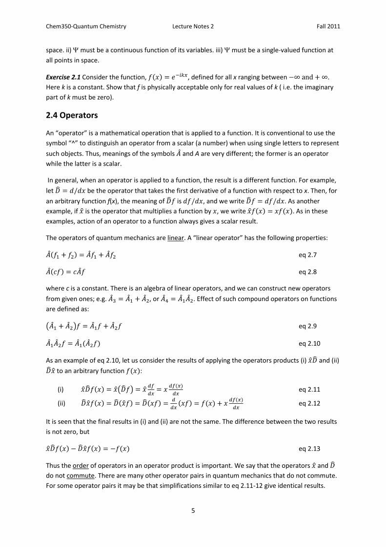
In general, when an operator is applied to a function, the result is a different function. For example,

let be the operator that takes the first derivative of a function with respect to x. Then, for

an arbitrary function f(x), the meaning of is , and we write . As another

example, if is the operator that multiplies a function by , we write . As in these

examples, action of an operator to a function always gives a scalar result.

The operators of quantum mechanics are linear. A “linear operator” has the following properties:

eq 2.7

eq 2.8

where c is a constant. There is an algebra of linear operators, and we can construct new operators

from given ones; e.g. , or . Effect of such compound operators on functions

are defined as:

eq 2.9

eq 2.10

As an example of eq 2.10, let us consider the results of applying the operators products (i) and (ii)

to an arbitrary function :

(i) eq 2.11

(ii) eq 2.12

It is seen that the final results in (i) and (ii) are not the same. The difference between the two results

is not zero, but

eq 2.13

Thus the order of operators in an operator product is important. We say that the operators and

do not commute. There are many other operator pairs in quantum mechanics that do not commute.

For some operator pairs it may be that simplifications similar to eq 2.11-12 give identical results.


6

Then we say that those two operators commute. For example, an arbitrary operator commutes

with all of its powers, .

Introducing the identity operator that multiplies a function by 1, eq 2.13 may be written as

eq 2.14

and we have the operator identity:

eq 2.15

For any two operators, the operator expression, , is called the “commutator” of and . Eq

2.15 shows that the commutator of and is not zero, i.e. these two operators do not commute. It

is common practice to omit the operator symbol “^” from letters (or numbers) representing

multiplication operators. For example, eq 2.15 is usually written as

eq 2.16

We will follow this practice.

Exercise 2.2 Find the commutator of: a) z3 and d/dz, b) z3 and /y (y and z are independent

variables). In each of these two cases, state whether the operators commute or not.

2.5 Eigenvalue-Eigenfunction Equation

Suppose that the result of operating on some function f by an operator is simply the initial function

multiplied by a special constant k:

Eigenvalue-eigenfunction equation for operator eq 2.17

If you compare the graphs of the functions f and kf (e.g. take a function of one variable), you will

convince yourself that the two graphs will look very similar, differing only in the scale of function

values. For example, they become zero at the same values of their variables, and they attain their

maxima and minima at the same points. Considering the fact that, in general, an operator transforms

a given function into a very different function, a function f that satisfies eq 2.17 is a very special one.

It turns out that for a given operator , there are many (in fact, infinitely many) functions (with

different values of k) obeying eq 2.17. The set of these special functions is called “eigenfunctions” of

the given operator (i.e. there is one operator , but there are infinitely many different functions,

each obeying eq 2.17 with a different value for k). Each eigenfunction is associated with a

corresponding value of k via eq 2.17. The set of different k values is called “eigenvalues” of the

operator . Eigenvalues of quantum mechanical operators are real numbers whereas there is no

such restriction for the eigenfunctions; i.e. the latter may be complex-valued.


7

If an eigenfunction f in eq 2.17 is replaced by cf where c is an arbitrary constant, the latter function

will also satisfy eq 2.17 with the same eigenvalue k due to the property given in eq 2.8.2 This

arbitrariness is removed by normalizing the eigenfunctions so that (see eq 2.4b): 3

eq 2.18

In the light of the operator concept, and the eigenvalue-eigenfunction equation 2.17, we can better

comprehend the Schrödinger equation, eq 2.1 (this is another example of main ideas vs. details).

When we decide on studying the properties of a given system (e.g. a single particle, or an atom with

many electrons, or a molecule, etc.), we always know the explicit expression for the Hamiltonian

operator of the system. is a function of the variables needed to locate spatial positions of

particles in the system. Thus, the Schrödinger equation is an eigenvalue-eigenfunction equation for

. The allowed energies of the system are eigenvalues of , and the state functions are

eigenfunctions of .

Orthogonality of eigenfunctions. Two different functions g and h of any number of variables are said

to be “orthogonal” if the following definite integral involving them vanishes:

Orthogonality eq 2.19

Let k1, k2, … be the various eigenvalues of a given operator , arranged in increasing order. The

corresponding eigenfunctions are denoted as f1, f2, … . It can be shown that any pair of functions

selected from the set of eigenfunctions satisfies eq 2.19

Orthogonality of eigenfunctions eq 2.20

We say that the eigenfunctions of the operator are orthogonal. If, in addition, the eigenfunctions

are normalized (eq 2.18), they are called “orthonormal” (a word derived from the two words:

orthogonal and normalized).

Exercise 2.3 Consider the function, g=c1f1+c2f2, where f1 and f2 are orthonormal functions. For g to be

normalized, what must be the relation between the constants c1 and c2?

Commuting and noncommuting operators. It has been mentioned in section 2.4 that while, in

general, two quantum mechanical operators do not commute, there are operator pairs that do

commute. For example, an operator always commutes with its powers, and any expression

involving its powers. Thus, you should easily show that commutes with itself, and also with 2, 3,

…, or with an operator such as =c1 +c22+c3

3 where c1, c2, and c3 are given constants. Another

important case is when the two operators depend on different independent variables. For example,

operator pairs such as and , (partial derivatives) always commute because x

and y are independent variables. Another example is where depends on spatial variables whereas

depends on “spin” (of an electron) variables. The latter type of variable (spin) will appear later in

this course. The spin variables are independent of the space variables, and therefore any operator

expression of spin variables always commutes with an operator of spatial variables.

2 In enumerating different eigenfunctions of eq 2.17, no distinction can be made between f and a multiple of it,

c f. In quantum mechanics, f and c f are always regarded as the “same” eigenfunction. 3 See section 2.2 for how to fill in “details” in the integrals of eqs 2.18-20.


8

The significance of commuting operators is that when two or more operators commute, they have

the same set of eigenfunctions.

Exercise 2.4 Show that if f is an eigenfunction of with eigenvalue k, (eq 2.17), then the same

function f is also an eigenfunction of the operator =c1 +c22+c3

3 with eigenvalue b=c1k+c2k2+c3k

3.

2.6 Rules for writing explicit expressions for quantum mechanical operators

Experimentally measurable properties of a system are called its “observables”. Quantum theory

associates each observable with a linear operator. Expressions for the operators are obtained from

known classical mechanical expressions for the observables, using simple rules. All classical quantities

must be expressed using Cartesian variables for the positions of particles, and their linear momenta.

The classical expression for the potential energy function, V, is used in quantum theory without any

modification. In all quantum chemical applications, V is a function of coordinates only.

We will use the standard symbol T for the classical kinetic energy. Let us consider a particle of mass

m, moving in 3D. T must be written in terms of the linear momentum, , of the particle before

converting T into a quantum operator. Linear momentum is a vector with Cartesian components:

. The classical kinetic energy of the particle is given by

where eq 2.21

In classical mechanics, the sum of the kinetic energy (expressed in terms of momenta) and the

potential energy of a material system is known as the hamiltonian of the system, denoted by the

standard symbol H; i.e. H=T+V. Classical H is a constant, equal to the total energy of the system: H=E.

For our single particle example, it is:

eq 2.22

Expressions for quantum operators are obtained from their classical counterparts by the following

rule: each Cartesian component of linear momentum in the classical expression is replaced by the

operator

eq 2.23

where and are constants, and (x,y,z) are the Cartesian coordinates of the

particle. The operator for is obtained by using eq 2.10

eq 2.24

The kinetic energy operator for a single particle in 3D space is thus

eq 2.25

and the explicit Hamiltonian operator is


9

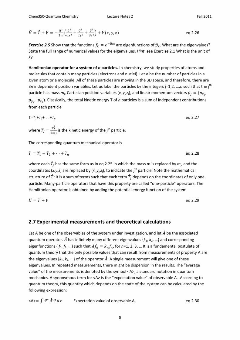
eq 2.26

Exercise 2.5 Show that the functions are eigenfunctions of . What are the eigenvalues?

State the full range of numerical values for the eigenvalues. Hint: see Exercise 2.1 What is the unit of

k?

Hamiltonian operator for a system of n particles. In chemistry, we study properties of atoms and

molecules that contain many particles (electrons and nuclei). Let n be the number of particles in a

given atom or a molecule. All of these particles are moving in the 3D space, and therefore, there are

3n independent position variables. Let us label the particles by the integers j=1,2, …,n such that the jth

particle has mass mj, Cartesian position variables (xj,yj,zj), and linear momentum vectors

. Classically, the total kinetic energy T of n particles is a sum of independent contributions

from each particle

T=T1+T2+ … +Tn eq 2.27

where is the kinetic energy of the jth particle.

The corresponding quantum mechanical operator is

eq 2.28

where each has the same form as in eq 2.25 in which the mass m is replaced by mj, and the

coordinates (x,y,z) are replaced by (xj,yj,zj), to indicate the jth particle. Note the mathematical

structure of it is a sum of terms such that each term depends on the coordinates of only one

particle. Many-particle operators that have this property are called “one-particle” operators. The

Hamiltonian operator is obtained by adding the potential energy function of the system

eq 2.29

2.7 Experimental measurements and theoretical calculations

Let A be one of the observables of the system under investigation, and let be the associated

quantum operator. has infinitely many different eigenvalues {k1, k2, …} and corresponding

eigenfunctions { f1, f2, …} such that , for n=1, 2, 3, … It is a fundamental postulate of

quantum theory that the only possible values that can result from measurements of property A are

the eigenvalues {k1, k2, …} of the operator . A single measurement will give one of these

eigenvalues. In repeated measurements, there might be dispersion in the results. The “average

value” of the measurements is denoted by the symbol <A>, a standard notation in quantum

mechanics. A synonymous term for <A> is the “expectation value” of observable A. According to

quantum theory, this quantity which depends on the state of the system can be calculated by the

following expression:

<A> Expectation value of observable A eq 2.30


10

where is a given normalized wavefunction for the state of interest (i.e. an allowed solution of the

Schrödinger equation 2.1). Evaluation of the integral in eq 2.30 proceeds in two steps: i) one first

simplifies the part as much as possible by using the given (i.e. known) expressions for the

operator and the state function ; ii) the resultant expression (i.e. a function) from the first step is

multiplied by , and then the integral is evaluated.

It should be noted that unless commutes with the Hamiltonian , the state function can not be

an eigenfunction of , and as a consequence, will be a different function than . In the special,

but important case when commutes with , will be proportional to one of the eigenfunctions

of with eigenvalue , which leads to the conclusion that = .4 In this case, the integral in eq

2.30 can be evaluated immediately

<A> eq 2.31

because is normalized. Thus repeated measurements of property A will all result with the same

value, , (i.e. no dispersion) when the associated operator commutes with the Hamiltonian

operator of the system. An example is the measurement of the energy, E, of the system in a given

stationary state. Since is one of the eigenfunctions of , say with eigenvalue En, every

measurement of E of the system in this state will yield the same energy En. The usual notation for the

average energy is <H>, rather than <E>.

Example 2.2 Calculate the average distance of the electron from the nucleus in H-atom for the

ground state of the electron (see Example 2.1 for the normalized ground state ).

Procedure: The observable is the distance of the electron from the nucleus. This is identified as the

variable in polar coordinates. Its average value is designated as < >. The associated operator is ; it

multiplies any function with : . The rest is a matter of evaluating a simple triple integral,

and can be done in a similar way to that in Example 2.1. You will obtain, < >=3a0/2=79.4 pm.

2.8 Expansion of into a Linear Combination of Eigenfunctions

Suppose that for a given state of the system is available as an explicit expression. For some

purposes in quantum theory, we wish to express it in the following special form

eq 2.32

where { f1, f2, …} are normalized eigenfunctions of an operator , and { c1, c2, …} are constants. It will

be assumed that explicit expressions for all of the eigenfunctions are given. The sum on the right side

is called “linear combination” of the functions { f1, f2, …}, and we say that we have “expanded” into

a linear combination of these functions. For the expression 2.32 is to be useful, we must know how

to calculate the coefficients from the given information. The orthogonality property (eq 2.20) of the

eigenfunctions makes this task easy. In order to use it, we multiply both sides of eq 2.32 by the

complex conjugate of one of the eigenfunctions , and integrate

4 See the part “commuting and noncommuting operators” in section 2.5.


11

eq 2.33

Among the many integrals on the right side, due to the orthogonality property of the eigenfunctions,

only one integral will be nonzero: the one with the nth coefficient cn. The nonzero integral,

because we are told that the eigenfunctions are normalized. Therefore, we can write

eq 2.34

Since by hypothesis the explicit expressions for both and are available, this definite integral can

be evaluated for n=1, 2, …, in succession, yielding numerical values of all coefficients in eq 2.32.5

Probability interpretation of (eq 2.5-2.6) is valid only if it is normalized: . We may

express the normalization condition in terms of the coefficients in eq 2.32 as follows. We replace

in the normalization integral by its expansion (eq 2.32), and use eq 2.34:6

Thus

eq 2.35

when in eq 2.32 is normalized.

It is of interest to express the average value of observable A (eq 2.30) in the given state in terms of

these coefficients since it leads to a theoretical prediction of the probability of observing each

eigenvalue kn of the operator . We first simplify the term in the integrand of eq 2.30 where

has the form in eq 2.32.

Then

Comparison with eq 2.34 shows that the value of each integral on the right side is simply cn*. Thus

we obtain the desired expression:

<A>= eq 2.36

If does not commute with , many of the coefficients calculated by eq 2.34 will not be zero. In this

case, the average value of observable A in the state is a weighted average of eigenvalues of the

associated operator . The weight factor of each eigenvalue is interpreted as the probability

of getting in a measurement of property A. As seen from eq 2.35, the sum of all probabilities is 1,

in agreement with the probability concept. On the other hand, if commutes with then must be

one of the eigenfunctions { f1, f2, …} of , e.g. for a given n, and because of the orthogonality

5 If the eigenfunctions and/or are complex-valued functions, values of the coefficients may be complex

numbers. 6 For any two complex numbers z1 and z2, one has the identities: (z1+z2)*=z1*+z2* and (z1z2)*=z1*z2*


12

property, eq 2.35 will give a nonzero result for only one coefficient: cn=1. This case has been

discussed previously (eq 2.31).

Exercise 2.6 Given

Assume that the particle is in a state with , where C is a constant. The

functions are normalized. In measurements of property A of the particle in this state, what are the

possible outcomes for A, and the probability of each outcome?

Additional Exercises for this part:

Problems 16, 17, 18, 21, 26 in Chapter 11 of Physical Chemistry (4th ed.) by Laidler, Meiser and

Sanctuary

Theoretical Foundation

Documents

Transcript of Theoretical Foundation