TheGaige - Pennsylvania State University

The Gaige Technology and Business

Innovation Building

Penn State Berks, Reading PA

Geothermal Redesign of the Gaige Building

Final Report: Architectural Engineering Senior Thesis

THE PENNSYLVANIA STATE UNIVERSITY

SCHREYER HONORS COLLEGE

DEPARTMENT OF ARCHITECTURAL ENGINEERING

Matthew T. Neal

Spring 2014

A thesis submitted in partial fulfillment of the requirements for

a baccalaureate degree in Architectural Engineering

with honors in Architectural Engineering

Reviewed and approved* by the following:

Stephen Treado

Associate Professor of Architectural Engineering

Thesis Supervisor

Richard Mistrick

Associate Professor of Architectural Engineering

Honors Advisor

*Signatures are on file in the Schreyer Honors College

Page i

Final Report

April 7th, 2014

Page i

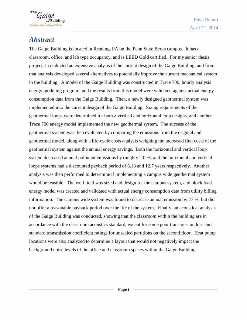
Abstract

The Gaige Building is located in Reading, PA on the Penn State Berks campus. It has a

classroom, office, and lab type occupancy, and is LEED Gold certified. For my senior thesis

project, I conducted an extensive analysis of the current design of the Gaige Building, and from

that analysis developed several alternatives to potentially improve the current mechanical system

in the building. A model of the Gaige Building was constructed in Trace 700, hourly analysis

energy modeling program, and the results from this model were validated against actual energy

consumption data from the Gaige Building. Then, a newly designed geothermal system was

implemented into the current design of the Gaige Building. Sizing requirements of the

geothermal loops were determined for both a vertical and horizontal loop designs, and another

Trace 700 energy model implemented the new geothermal system. The success of the

geothermal system was then evaluated by comparing the emissions from the original and

geothermal model, along with a life-cycle costs analysis weighing the increased first costs of the

geothermal system against the annual energy savings. Both the horizontal and vertical loop

system decreased annual pollutant emissions by roughly 2.0 %, and the horizontal and vertical

loops systems had a discounted payback period of 6.13 and 12.7 years respectively. Another

analysis was then performed to determine if implementing a campus wide geothermal system

would be feasible. The well field was sized and design for the campus system, and block load

energy model was created and validated with actual energy consumption data from utility billing

information. The campus wide system was found to decrease annual emission by 27 %, but did

not offer a reasonable payback period over the life of the system. Finally, an acoustical analysis

of the Gaige Building was conducted, showing that the classroom within the building are in

accordance with the classroom acoustics standard, except for some poor transmission loss and

standard transmission coefficient ratings for unsealed partitions on the second floor. Heat pump

locations were also analyzed to determine a layout that would not negatively impact the

background noise levels of the office and classroom spaces within the Gaige Building.

Final Report

April 7th, 2014

Page ii

Table of Contents

Abstract ............................................................................................................................................ i

Acknowledgements ...................................................................................................................... xiv

Chapter 1: Executive Summary ...................................................................................................... 1

Chapter 2: Existing Conditions: ...................................................................................................... 2

2.1: Building Overview and Background .................................................................................... 2

2.2: Existing Mechanical System Overview ............................................................................... 3

2.3: Mechanical System Design Requirements ........................................................................... 4

2.3.1: Design Objectives ......................................................................................................... 4

2.3.2: Energy Sources and Rates............................................................................................. 5

2.3.3: Design Conditions......................................................................................................... 6

2.3.4: Ventilation Requirements ............................................................................................. 8

2.3.5: Heating and Cooling Loads .......................................................................................... 9

2.3.6: Annual Energy Use ..................................................................................................... 10

2.4: Design Load Estimation ..................................................................................................... 13

2.4.1: Model Design Approach ............................................................................................. 14

2.4.2: System Design Assumptions ...................................................................................... 15

2.4.3: Model Comparison with Utility Data ......................................................................... 19

2.4.4: Model Validation ........................................................................................................ 21

2.5: Existing Annual Costs, Energy Consumption, and Emissions .......................................... 23

2.5.1: Annual Energy Costs .................................................................................................. 24

2.5.2: Site versus Source Energy Comparison ...................................................................... 25

Final Report

April 7th, 2014

Page iii

2.5.3: Total Annual Emission Rates ..................................................................................... 27

Chapter 3: Mechanical Depth: Geothermal Analysis .................................................................. 29

3.1 Geothermal Analysis of the Gaige Building ....................................................................... 30

3.1.1: Design Objectives ....................................................................................................... 30

3.1.2: Geothermal System Sizing and Calculations .............................................................. 32

3.1.3: Geothermal System Layout—Vertical Bore Option ................................................... 40

3.1.4: Geothermal System Layout—Horizontal Bore Option .............................................. 44

3.1.5: Proposed System Configuration ................................................................................. 45

3.1.6: Building Piping Layout ............................................................................................... 47

3.1.7: Geothermal Equipment Selection ............................................................................... 51

3.1.8: Dedicated Outdoor Air System ................................................................................... 57

3.1.9: Annual Energy and Cost Analysis .............................................................................. 58

3.1.10: Source Energy Consumption and Emissions ............................................................ 61

3.1.11: Life Cycle Cost Analysis .......................................................................................... 64

3.2: Campus-wide Geothermal System Analysis ...................................................................... 68

3.2.1: Campus-wide Geothermal Motivation........................................................................ 68

3.2.2: Campus Wide Load Analysis ..................................................................................... 69

3.2.3: Energy Analysis of Campus Buildings ....................................................................... 70

3.2.4: Modeling Validation of Overall Campus Energy Consumption ................................ 74

3.2.5: Geothermal Modeling of Overall Campus.................................................................. 76

3.2.6: Campus Wide Geothermal Sizing and Layout ........................................................... 77

3.2.7: Cost and Energy Analysis ........................................................................................... 80

Final Report

April 7th, 2014

Page iv

Chapter 4: Acoustical Breadth ...................................................................................................... 88

4.1: Honors Work: Acoustics Performance of the Gaige Building ........................................... 88

4.1.1: Room Acoustics Performance .................................................................................... 88

4.1.2: Sound Isolation Performance ...................................................................................... 94

4.2: Heat Pump Noise Control and Isolation........................................................................... 100

4.2.1: Heat Pump Location Options .................................................................................... 101

4.2.2: Analysis of Sound Isolation through Partitions ........................................................ 106

4.2.3: Analysis of Air Noise through Diffusers .................................................................. 106

Chapter 5: Construction Breadth ................................................................................................ 110

4.1: Geothermal Bore Cost Evaluation ................................................................................... 110

4.1.1: Vertical Bore Cost Estimation .................................................................................. 111

4.1.2: Horizontal Bore Cost Estimation .............................................................................. 113

4.1.3: Comparison of Vertical Bore to Horizontal Bore Costs ........................................... 115

4.2: Gaige Building Geothermal—Initial Costs ...................................................................... 115

4.2.1: Savings from Original Design .................................................................................. 115

4.2.2: Initial Costs for Vertical Bore Design ...................................................................... 116

4.2.3: Initial Costs for Horizontal Bore Design .................................................................. 117

Chapter 6: Conclusions ............................................................................................................... 118

References ................................................................................................................................... 120

Appendix A: Building Pump Head Loss Calculations .............................................................. 121

Appendix B: Horizontal Geothermal Pump Head Calculations ................................................ 122

Appendix C: Emissions Factors ................................................................................................. 124

Final Report

April 7th, 2014

Page v

Appendix D: Original Mechanical System Costs ...................................................................... 125

Appendix E: Campus Geothermal Well Field Costs ................................................................. 127

Appendix F: Costs of Vertical Geothermal System ................................................................... 129

Appendix G: Costs of Horizontal Geothermal System .............................................................. 132

Appendix H: Acoustics Reference Data .................................................................................... 135

Appendix I: Ductwork Noise Outputs from Dynasonics ........................................................... 138

Final Report

April 7th, 2014

Page vi

List of Figures

Figure 1: The Gaige Building ........................................................................................................ 1

Figure 2: Annual energy distribution as calculated by the Trace 700 ......................................... 11

Figure 3: Actual utility costs for the Gaige Building from May 2012 to May 2013 ................... 12

Figure 4: Actual electricity costs for the Gaige Building from May 2012 to May 2013 ............. 13

Figure 5: Actual natural gas utility costs for the Gaige Building from May 2012 to May 2013 . 13

Figure 6: Actual vs. Modeled electricity consumption on a monthly basis ................................. 20

Figure 7: Actual vs. Modeled natural gas consumption on a monthly basis ............................... 21

Figure 8: Comparison of actual monthly electricity consumption with results from the validated

Trace 700 model ........................................................................................................................... 22

Figure 9: A comparison between the utility data for natural gas usage in the ............................. 23

Figure 10: The monthly energy costs for the Gaige Building for electricity and natural gas. ..... 24

Figure 11: A figure showing the comparison of heating energy (natural gas) to ........................ 26

Figure 12: A figure showing the comparison of heating energy (natural gas) to ........................ 26

Figure 13: A Graphs showing the annual emission of each pollutant the Gaige Building by

energy source ................................................................................................................................ 28

Figure 14: Penn State Berks campus map showing the Gaige Building and ............................... 29

Figure 15: A graph breaking down the monthly energy consumption of the .............................. 31

Figure 16: Graph from chapter 34 of ASHRAE Applications to help calculate G factors .......... 36

Figure 17: Table six from chapter 34 of ASHRAE Applications used to calculated bore thermal

resistance ....................................................................................................................................... 37

Figure 18: Undisturbed ground temperatures for the United States, Reading, PA show at red dot

....................................................................................................................................................... 38

Final Report

April 7th, 2014

Page vii

Figure 19: Specifications of a vertical well designed for the Gaige Building ............................. 42

Figure 20: Site layout of the vertical geothermal well field ........................................................ 43

Figure 21: Location of the geothermal well field with respect to the rest of campus .................. 43

Figure 22: A horizontal loop geothermal pipe, typical section for one loop per pipe, ASHRAE

Application, Ch 34 ........................................................................................................................ 44

Figure 23: Proposed configuration of the Gaige Building’s horizontal loop geothermal system 45

Figure 24: A schematic of the piping arrangement in the Gaige Building’s proposed geothermal

design ............................................................................................................................................ 46

Figure 25: A diagram of the first floor HVAC zoning and piping distribution ............................ 48

Figure 26: A diagram of the second floor HVAC zoning and piping distribution ...................... 49

Figure 27: A diagram of the third floor HVAC zoning and piping distribution .......................... 50

Figure 28: A picture of a Bell and Gossett, base mounted centrifugal pump, series e-1510 ....... 52

Figure 29: Pump selection diagram provided by Bell and Gossett to assist in pump sizing.

Vertical geothermal pump is shown in red and horizontal geothermal loop pump is shown in

green .............................................................................................................................................. 53

Figure 30: Pump curve for the selected vertical bore geothermal pump shown at operating

conditions in red ............................................................................................................................ 53

Figure 31: The pump curves shown for the horizontal loop geothermal field pump, operating

conditions shown .......................................................................................................................... 54

Figure 32: Pump selection diagram provided by Bell and Gossett .............................................. 55

Figure 33: Pump operating curves for the building pumps, shown at operating conditions in red

....................................................................................................................................................... 56

Figure 34: A sketch of the water source heat pumps selected from Carrier, both horizontal and

vertical unit shown ........................................................................................................................ 57

Final Report

April 7th, 2014

Page viii

Figure 35: Monthly electricity costs for the original and geothermal redesign of the Gaige

Building......................................................................................................................................... 58

Figure 36: Monthly natural gas costs for the original and geothermal redesign of the Gaige

Building......................................................................................................................................... 59

Figure 37: Monthly energy costs for the original and geothermal redesign of the Gaige Building

....................................................................................................................................................... 59

Figure 38: Monthly electricity consumption of the Gaige Building with the original and

geothermal redesign ...................................................................................................................... 60

Figure 39: Monthly natural gas consumption of the Gaige Building with the original and


Figure 40: A graph showing the annual pollutants from the of the original Gaige Building’s

mechanical system ........................................................................................................................ 61

Figure 41: A graph showing the annual pollutants from the geothermal system for the Gaige

Building......................................................................................................................................... 62

Figure 42: Site energy consumption for the Gaige Building with a geothermal system ............. 63

Figure 43: Source energy consumption for the Gaige Building with a geothermal system ........ 63

Figure 44: Life cycle cost analysis of the vertical well system for the Gaige Building .............. 66

Figure 45: The life cycle cost analysis for the horizontal loop option for the Gaige Building ... 67

Figure 46: Total monthly energy costs for the Penn State Berks campus by specific building .. 69

Figure 47: Total monthly electricity costs for the Penn State Berks campus by specific building

....................................................................................................................................................... 70

Figure 48: Total monthly natural gas costs for the Penn State Berks campus by specific building

....................................................................................................................................................... 70

Figure 49: Annual energy cost comparison between the original campus and the geothermal

redesign of the campus.................................................................................................................. 77

Final Report

April 7th, 2014

Page ix

Figure 50: A layout of the overall geothermal system to serve the campus. Well field piping is

shown in blue and red, and orange piping is part of the campus distribution piping. Pumps are

shown as orange boxes.................................................................................................................. 79

Figure 51: A comparison between the required geothermal lengths for separate and centralized

geothermal systems ....................................................................................................................... 80

Figure 52: Estimated annual emission from the current campus system for Penn State Berks ... 81

Figure 53: Estimated Annual emission from the geothermal redesign of the Penn State Berks

campus .......................................................................................................................................... 81

Figure 54: Two AE 309 students who helped with the measurements, using the B&K 2250

sound level analyzer ...................................................................................................................... 89

Figure 55: Myself using the B&K 2250 sound level analyzer..................................................... 89

Figure 56: Aharon and Cory setting up a speaker for the transmission loss and reverberation

time measurements........................................................................................................................ 89

Figure 57: T30 measurements of classrooms in the Gaige Building that are less than 10,000

cubic feet ....................................................................................................................................... 91

Figure 58: T30 measurements of classrooms in the Gaige Building that are greater than 10,000

cubic feet ....................................................................................................................................... 91

Figure 59: Background noise levels in the six classroom spaces. The target NC-35 is shown in

red ................................................................................................................................................. 93

Figure 60: Typical measurement setup to take transmission loss measurement of a partition

between rooms .............................................................................................................................. 95

Figure 61: ATL measurement results for the partition between classroom 120 and 121, with an

ASTC of 46 ................................................................................................................................... 96


ASTC of 49 ................................................................................................................................... 97

Final Report

April 7th, 2014

Page x


ASTC of 40 ................................................................................................................................... 98


ASTC of 38 ................................................................................................................................... 98

Figure 65: One of the low performing walls, shown where it is built into a window glazing

system ........................................................................................................................................... 99

Figure 66: The gap in the same wall shown in figure 65, where the wall meets the window ..... 99

Figure 67: Source location of instructor shown in red, and receiver locations shown in blue,

typical classroom ........................................................................................................................ 101

Figure 68: A grid response showing the A-weighted sound pressure levels when .................... 103

Figure 69: The geometrical model of the two classroom spaces with sources and receivers

shown .......................................................................................................................................... 104

Figure 70: A grid response showing the resulting A-weighted sound pressure levels in both

classrooms ................................................................................................................................... 105

Figure 71: NC plot of background noise level from heat pump duct work for a typical classroom

..................................................................................................................................................... 107

Figure 72: NC plot of background noise level from heat pump duct work for a typical office 109

Figure 73: A graph showing RS Means data for pile boring costs as bore diameter changes ... 112

Figure 74: A pie chart showing the percentage breakdown of costs for a vertical geothermal well

that is 300’ deep .......................................................................................................................... 112

Figure 75: A pie chart showing the breakdowns between trenching and piping costs for a 800’

horizontal loop ............................................................................................................................ 114

Final Report

April 7th, 2014

Page xi

List of Tables

Table 1: Energy rates used for the cost analysis for the Gaige Building, used in the .................... 5

Table 2: Energy rates that have been calculated using data provided from ................................... 6

Table 3: Design set points for the Gaige Building for different spatial types and seasons ........... 7

Table 4: Data used for the weather design conditions from the design of the ............................... 7

Table 5: Weather data that is used in the final modeling of the Gaige building in this report ...... 7

Table 6: Summary of the ventilation calculations performed for the Gaige Building's three

RTU's .............................................................................................................................................. 8

Table 7: A summary of the loads calculated from the Trace 700 Model in Technical Report Two

......................................................................................................................................................... 9

Table 8: A comparison of the loads calculated from the Trace 700 model ................................. 10

Table 9: A comparison of the annual energy usage calculated from the Trace 700 model and the

Carrier HAP Model ....................................................................................................................... 11

Table 10: Electrical equipment loads used in the model on a W/SF basis, with the exception of

the kitchen area ............................................................................................................................. 17

Table 11: Miscellaneous electrical loads found throughout the building, provided H.F. Lenz

Company ....................................................................................................................................... 17

Table 12: Thermal resistance values for different construction types used in the Gaige Building

....................................................................................................................................................... 18

Table 13: Annual energy costs for both the Trace 700 model and actual data from the Gaige

Building......................................................................................................................................... 20

Table 14: A summary of the annual energy costs in the validated model of the Gaige Building,

....................................................................................................................................................... 25

Table 15: Table summarizing the total annual emissions of the Gaige Building ........................ 27

Final Report

April 7th, 2014

Page xii

Table 16: From ASHRAE HVAC Application, chapter 34, used to find short circuit heat loss

factor ............................................................................................................................................. 33

Table 17: A table summarizing the geothermal length calculations for the Gaige Building ........ 40

Table 18: A table showing the required number of bores to serve the Gaige Building, depending

upon bore depth............................................................................................................................. 41

Table 19: A summary of how differing loop lengths are used to meet the horizontal loop length

requirements .................................................................................................................................. 45

Table 20: Head loss calculation summary table for the geothermal pump in the Gaige Building

....................................................................................................................................................... 51

Table 21: A table showing the percent decrease in emissions from switching to a geothermal

system ........................................................................................................................................... 62

Table 22: Increased first costs for the vertical well geothermal layout ....................................... 65

Table 23: Increased first costs for the horizontal loop geothermal system.................................. 65

Table 24: Rates using in the life cycle costs analyses for the Gaige Building ............................ 66

Table 25: A list of the Berks campus building and their occupancy types .................................. 72

Table 26: Summary of the percentage of overall fuel use for the heating, cooling, and ventilation

of building that use both natural gas and electricity as an energy source ..................................... 73

Table 27: A summary of the percentage of electricity used for heating, cooling, and ventilation

for the electric only service building on the Penn State Berks campus ........................................ 73

Table 28: Overall annual energy use estimates for each campus building .................................. 74

Table 29: Percentage deviations between EIA data targets for annual energy consumption and

Trace 700 results ........................................................................................................................... 75

Table 30: Required geothermal total well lengths for the campus-wide geothermal system ...... 78

Final Report

April 7th, 2014

Page xiii

Table 31: Annual pollutant emissions for each design, and the percentage reduction from the


Table 32: Estimate of initial costs for heat pumps, heat pump piping, and building water pumps

for the campus ............................................................................................................................... 83

Table 33: Estimates for the initial costs of DOAS units and building maintenance for the campus

....................................................................................................................................................... 84

Table 34: Overall increase in first costs for the campus geothermal system ............................... 85

Table 35: A table summarizing the simple payback period as the number of bores is adjusted

with load diversity......................................................................................................................... 86

Table 36: A tale showing how an added first cost savings can impact the campus-wide system’s

payback period .............................................................................................................................. 87

Table 37: Costs estimate for a vertical geothermal well, based upon a 300’ deep well ............ 111

Table 38: Cost estimates for a horizontal geothermal loop that is 800 feet long ....................... 113

Table 39: A summary of the cost per horizontal loop, as loop length is adjusted ..................... 114

Table 40: Summary of cost savings that can be realized from the original Gaige Building’s

design .......................................................................................................................................... 116

Table 41: A summary of the initial first costs increase for the vertical geothermal system ...... 117

Table 42: A summary of the overall increased first costs for the horizontal loop geothermal

design .......................................................................................................................................... 117

Final Report

April 7th, 2014

Page xiv

Acknowledgements

Insert Text Here

Final Report

April 7th, 2014

Page 1

Final Report

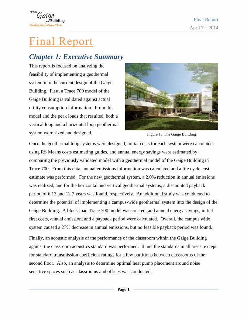
Chapter 1: Executive Summary

This report is focused on analyzing the

feasibility of implementing a geothermal

system into the current design of the Gaige

Building. First, a Trace 700 model of the

Gaige Building is validated against actual

utility consumption information. From this

model and the peak loads that resulted, both a

vertical loop and a horizontal loop geothermal

system were sized and designed.

Once the geothermal loop systems were designed, initial costs for each system were calculated

using RS Means costs estimating guides, and annual energy savings were estimated by

comparing the previously validated model with a geothermal model of the Gaige Building in

Trace 700. From this data, annual emissions information was calculated and a life cycle cost

estimate was performed. For the new geothermal system, a 2.0% reduction in annual emissions

was realized, and for the horizontal and vertical geothermal systems, a discounted payback

period of 6.13 and 12.7 years was found, respectively. An additional study was conducted to

determine the potential of implementing a campus-wide geothermal system into the design of the

Gaige Building. A block load Trace 700 model was created, and annual energy savings, initial

first costs, annual emission, and a payback period were calculated. Overall, the campus wide

system caused a 27% decrease in annual emissions, but no feasible payback period was found.

Finally, an acoustic analysis of the performance of the classroom within the Gaige Building

against the classroom acoustics standard was performed. It met the standards in all areas, except

for standard transmission coefficient ratings for a few partitions between classrooms of the

second floor. Also, an analysis to determine optimal heat pump placement around noise

sensitive spaces such as classrooms and offices was conducted.

Figure 1: The Gaige Building

Final Report

April 7th, 2014

Page 2

Chapter 2: Existing Conditions:

2.1: Building Overview and Background

The Gaige Technology and Business Innovation Building is a 64,000 SF building located in

Reading, PA, on the Berks commonwealth campus of Penn State University. The Gaige

Building is a host of many functions, but primarily, it is used as classroom, office, and lab space

for the college’s engineering, business, and hotel and restaurant management programs.

The Gaige Building is three stories tall, and it was constructed between April 2010 and

November 2011. It was operated on a design-bid-build project delivery method, and had a full

range of consulting services, from cost-estimating to A-V consulting. Functionally, the first

floor contains classroom and lab spaces primarily, with a large area for studying and relaxing

called the Learning Loft. Once you move to the second floor, you see the same classroom and

lab emphasis, but a corridor on the east-west wing of the building provides a large amount of

conference and office space.

Once you move to the third floor, the east-west wing of the building is capped off at two stories,

but the north-sound wing continues up to three stories to accommodate one more classroom

space and ample office and conference space. The exterior of the building consists of weather-

resistant terracotta panel, metal framed exterior glazing and curtain wall systems, and precast

concrete panels. Together, all of these building elements provide an aesthetically pleasing, but

sealed and energy efficient building façade and enclosure. More information on the architecture

of the building can be found in the building statistics report performed on the Gaige Building

through this same thesis project.

Final Report

April 7th, 2014

Page 3

2.2: Existing Mechanical System Overview

The Gaige Building has three main root top units (RTU-1, RTU-2, and RTU-3) that provide

ventilation, conditioning, and exhaust for the majority of the spaces within the building’s design.

The units are sized to 20,500 CFM, 14,000 CFM, and 12,500 CFM respectively. Each of these

units serve a variety of spaces within the first, second, and third floors of the building. Air is

supplied from the roof top units at a supply temperature of 55 degrees, and it is ducted

throughout the building.

At the individual spaces, variable air volume boxes are provided for each zone. The VAV box

takes the 55 degree air, and varies the volume of air being supplied to the space to meet the

cooling requirement of the space at the current time. The load is monitored by a thermostat

located in each of the zones separately. CO2 and occupancy sensors also are coordinated with

the VAV boxes to allow for a reduction in outside air required to be supplied to each space. A

minimum set point prevents the VAV box from supplying air less than the minimum outside air

requirement for the space. A reheat coil prevents from overcooling the space when providing

minimum outside air at a time when cooling requirements are reduced.

Two 1300 MBH boilers provide the hot water service for the building and all mechanical heating

requirements. Four split system air conditioners are required to provide individual space cooling

for the telecom/data rooms in the building, and one computer room air conditioner is required for

the IT storage and equipment room, also supplied with an air-cooled chiller. Unit heaters are

provided throughout the building as needed in semi-heated spaces, such as the vestibules at the

building entrances.

Finally, the heating loads for the building are met by radiant-heating panels and fin-tube heat

exchangers placed at exterior walls of spaces that don’t experience a year round cooling load.

This allows for simultaneous heating and cooling throughout the building in spaces that contain

these heating elements. Although it provides poor energy efficiency, the VAV boxes are

equipped with reheat coils, so some heating in spaces without panes or fin-tubes could

potentially have some heating capacity, but that is not the primary design intent.

Final Report

April 7th, 2014

Page 4

2.3: Mechanical System Design Requirements

In this section of technical report three, an extensive analysis of the mechanical system of the

Gaige Building, at Penn State’s Berks Commonwealth Campus, is conducted. The design

focuses and goals will be initially stated, and then, all aspects of the mechanical system within

the Gaige Building will be discussed and analyzed. First, the objectives of the Gaige Building’s

design will be highlighted, as well as the energy sources that were present at the building’s site.

Then, the ventilation system of the building will be discussed. Finally, the heating and cooling

loads for the building and the heating and cooling systems will be presented. Schematics of

major water and air flow systems will be given to provide an overall graphic representation of

system operation.

2.3.1: Design Objectives

One of the main focuses of the Gaige Building was the need for energy performance. As a Penn

State Building, it was expected that The Gaige Building would underperform an ASHRAE

Standards baseline building by at least 30%. This could be accomplished through the envelope

construction of the building as well as the mechanical system used by the building. This need for

energy efficiency led to a decision to incorporate very high performance windows and glazing

into the façade of the building, a step towards the 30% reduction expectation. As well, the

rooftop units for the Gaige Building are each equipped with energy recovery wheels that help to

pre-heat outside air in the winter with exhaust air, or pre-cool in the summer.

As well, since the Gaige Building is simply a standalone classroom building, all of the heating

and cooling systems are provided from boiler and air-cooled chillers on-site. As a result of the

lower loads associated with this type and size of building, a centralized heating boiler plant is

used, but all cooling required is provided by separate systems. Each rooftop unit is equipped

with internal equipment that provides the necessary cooling, and the individual air-conditioning

units are connected to air-cooled chillers that provide the cooling needed for each unit.

Final Report

April 7th, 2014

Page 5

The final key design objective was water efficiency throughout the Gaige Building. To

accomplish this goal, the Gaige Building incorporates a rainwater harvesting and storage system

that provides for nearly 100% of the building’s non-potable water usage.

Overall, the Gaige Building is designed to be a building that is a landmark for the Penn State

Berks campus. It is a building unlike any other on campus. It acts as a showcase for students, a

standard for the building community, and an educational tool for the Reading community. With

its energy efficiency, water efficiency, and status in the area, it will be a landmark for much of

the future to come. The Gaige Building, as it educates students at the Penn State Berks campus,

will be long remembered.

2.3.2: Energy Sources and Rates

For the Gaige Building, the two sources of energy used in the mechanical system are natural gas

and electricity. Natural gas is used primarily for the two boilers that provide the hot water for

the heating coils in the rooftop units, auxiliary coils in the VAV units, and radiant and fin-tube

heaters throughout the building. Electricity is the main utility used by the Gaige Building, and it

is used for all internal building operations and cooling. All cooling units (the rooftop units and

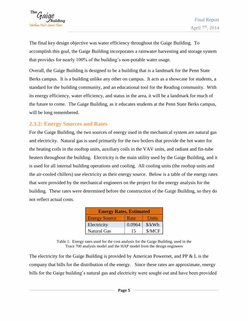
the air-cooled chillers) use electricity as their energy source. Below is a table of the energy rates

that were provided by the mechanical engineers on the project for the energy analysis for the

building. These rates were determined before the construction of the Gaige Building, so they do

not reflect actual costs.

Energy Rates, Estimated

Energy Source Rate Units

Electricity 0.0964 $/kWh

Natural Gas 15 $/MCF

Table 1: Energy rates used for the cost analysis for the Gaige Building, used in the

Trace 700 analysis model and the HAP model from the design engineers

The electricity for the Gaige Building is provided by American Powernet, and PP & L is the

company that bills for the distribution of the energy. Since these rates are approximate, energy

bills for the Gaige building’s natural gas and electricity were sought out and have been provided

Final Report

April 7th, 2014

Page 6

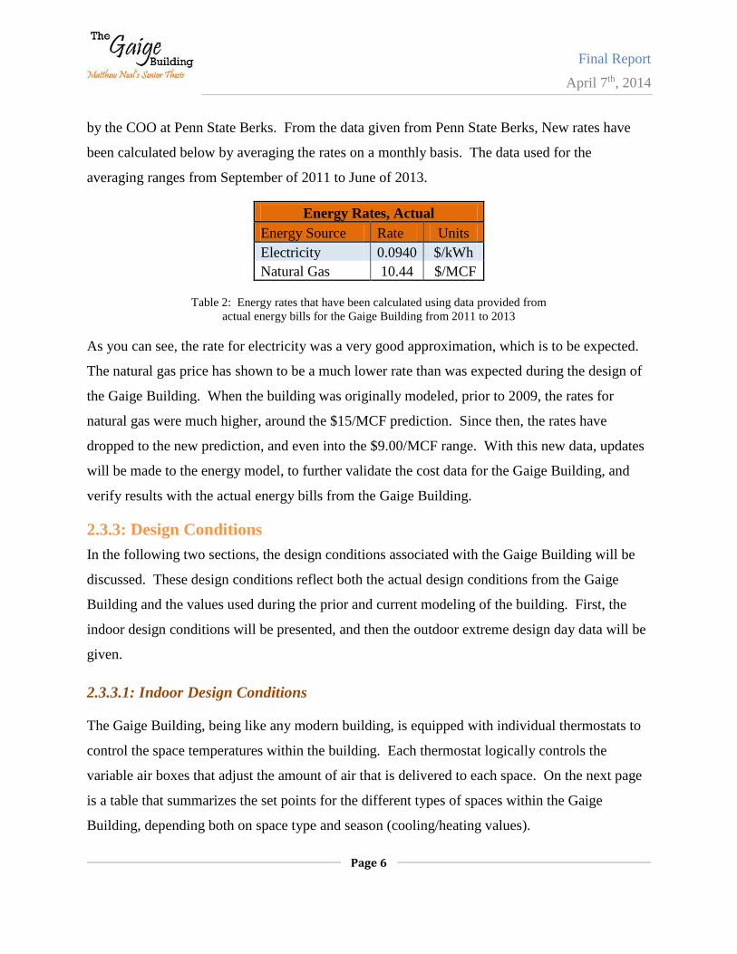
by the COO at Penn State Berks. From the data given from Penn State Berks, New rates have

been calculated below by averaging the rates on a monthly basis. The data used for the

averaging ranges from September of 2011 to June of 2013.

Energy Rates, Actual

Energy Source Rate Units

Electricity 0.0940 $/kWh

Natural Gas 10.44 $/MCF

Table 2: Energy rates that have been calculated using data provided from

actual energy bills for the Gaige Building from 2011 to 2013

As you can see, the rate for electricity was a very good approximation, which is to be expected.

The natural gas price has shown to be a much lower rate than was expected during the design of

the Gaige Building. When the building was originally modeled, prior to 2009, the rates for

natural gas were much higher, around the $15/MCF prediction. Since then, the rates have

dropped to the new prediction, and even into the $9.00/MCF range. With this new data, updates

will be made to the energy model, to further validate the cost data for the Gaige Building, and

verify results with the actual energy bills from the Gaige Building.

2.3.3: Design Conditions

In the following two sections, the design conditions associated with the Gaige Building will be

discussed. These design conditions reflect both the actual design conditions from the Gaige

Building and the values used during the prior and current modeling of the building. First, the

indoor design conditions will be presented, and then the outdoor extreme design day data will be

given.

2.3.3.1: Indoor Design Conditions

The Gaige Building, being like any modern building, is equipped with individual thermostats to

control the space temperatures within the building. Each thermostat logically controls the

variable air boxes that adjust the amount of air that is delivered to each space. On the next page

is a table that summarizes the set points for the different types of spaces within the Gaige

Building, depending both on space type and season (cooling/heating values).

Final Report

April 7th, 2014

Page 7

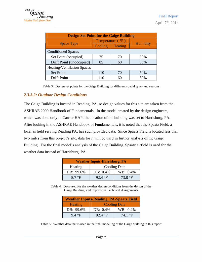
Design Set Point for the Gaige Building

Space Type Temperature ( °F )

Humidity Cooling Heating

Conditioned Spaces

Set Point (occupied) 75 70 50%

Drift Point (unoccupied) 85 60 50%

Heating/Ventilation Spaces

Set Point 110 70 50%

Drift Point 110 60 50%

Table 3: Design set points for the Gaige Building for different spatial types and seasons

2.3.3.2: Outdoor Design Conditions

The Gaige Building is located in Reading, PA, so design values for this site are taken from the

ASHRAE 2009 Handbook of Fundamentals. In the model created by the design engineers,

which was done only in Carrier HAP, the location of the building was set to Harrisburg, PA.

After looking in the ASHRAE Handbook of Fundamentals, it is noted that the Spaatz Field, a

local airfield serving Reading PA, has such provided data. Since Spaatz Field is located less than

two miles from this project’s site, data for it will be used in further analysis of the Gaige

Building. For the final model’s analysis of the Gaige Building, Spaatz airfield is used for the

weather data instead of Harrisburg, PA.

Weather Inputs-Harrisburg, PA

Heating Cooling Data

DB: 99.6% DB: 0.4% WB: 0.4%

8.7 °F 92.4 °F 73.8 °F

Table 4: Data used for the weather design conditions from the design of the

Gaige Building, and in previous Technical Assignments

Weather Inputs-Reading, PA-Spaatz Field

Heating Cooling Data

DB: 99.6% DB: 0.4% WB: 0.4%

9.4 °F 92.4 °F 74.1 °F

Table 5: Weather data that is used in the final modeling of the Gaige building in this report

Final Report

April 7th, 2014

Page 8

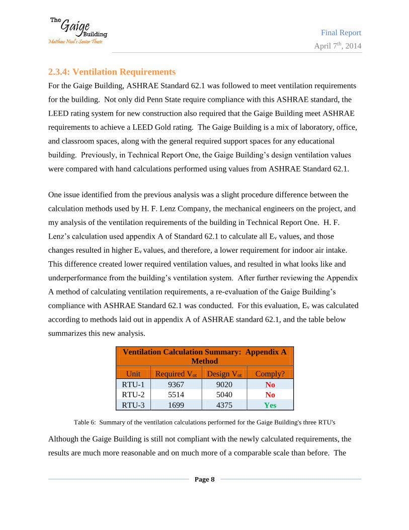
2.3.4: Ventilation Requirements

For the Gaige Building, ASHRAE Standard 62.1 was followed to meet ventilation requirements

for the building. Not only did Penn State require compliance with this ASHRAE standard, the

LEED rating system for new construction also required that the Gaige Building meet ASHRAE

requirements to achieve a LEED Gold rating. The Gaige Building is a mix of laboratory, office,

and classroom spaces, along with the general required support spaces for any educational

building. Previously, in Technical Report One, the Gaige Building’s design ventilation values

were compared with hand calculations performed using values from ASHRAE Standard 62.1.

One issue identified from the previous analysis was a slight procedure difference between the

calculation methods used by H. F. Lenz Company, the mechanical engineers on the project, and

my analysis of the ventilation requirements of the building in Technical Report One. H. F.

Lenz’s calculation used appendix A of Standard 62.1 to calculate all Ev values, and those

changes resulted in higher Ev values, and therefore, a lower requirement for indoor air intake.

This difference created lower required ventilation values, and resulted in what looks like and

underperformance from the building’s ventilation system. After further reviewing the Appendix

A method of calculating ventilation requirements, a re-evaluation of the Gaige Building’s

compliance with ASHRAE Standard 62.1 was conducted. For this evaluation, Ev was calculated

according to methods laid out in appendix A of ASHRAE standard 62.1, and the table below

summarizes this new analysis.

Ventilation Calculation Summary: Appendix A

Method

Unit Required Vot Design Vot Comply?

RTU-1 9367 9020 No

RTU-2 5514 5040 No

RTU-3 1699 4375 Yes

Table 6: Summary of the ventilation calculations performed for the Gaige Building's three RTU's

Although the Gaige Building is still not compliant with the newly calculated requirements, the

results are much more reasonable and on much more of a comparable scale than before. The

Final Report

April 7th, 2014

Page 9

value for Ep, the fraction of primary air to discharge air in the ventilation zone, was assumed to

be 1.0 in this calculation, which resulted in Fa, Fb, and Fc to have the value of 1.0 as well.

Despite the system’s underperformance, the required changes would be very minimal to

compensate for the differences. The differences, because of their small relative size, are

probably due to different area measurements or some other similar deviation.

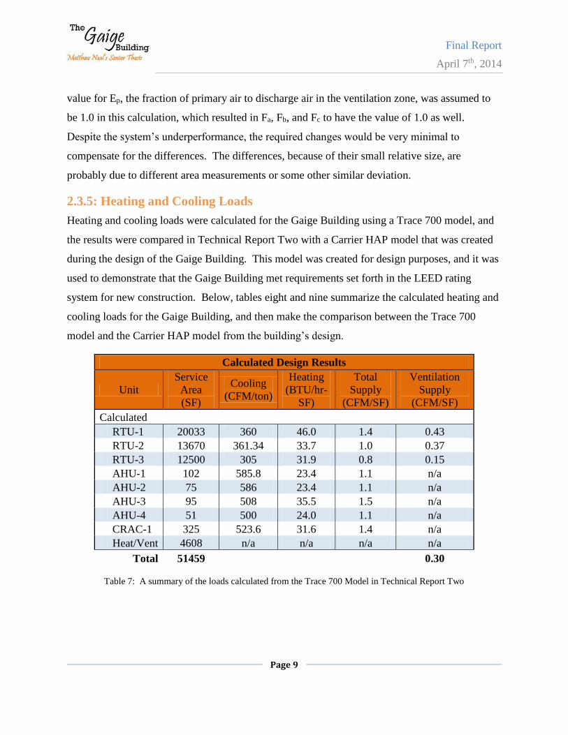
2.3.5: Heating and Cooling Loads

Heating and cooling loads were calculated for the Gaige Building using a Trace 700 model, and

the results were compared in Technical Report Two with a Carrier HAP model that was created

during the design of the Gaige Building. This model was created for design purposes, and it was

used to demonstrate that the Gaige Building met requirements set forth in the LEED rating

system for new construction. Below, tables eight and nine summarize the calculated heating and

cooling loads for the Gaige Building, and then make the comparison between the Trace 700

model and the Carrier HAP model from the building’s design.

Calculated Design Results

Unit

Service

Area

(SF)

Cooling

(CFM/ton)

Heating

(BTU/hr-

SF)

Total

Supply

(CFM/SF)

Ventilation

Supply

(CFM/SF)

Calculated

RTU-1 20033 360 46.0 1.4 0.43

RTU-2 13670 361.34 33.7 1.0 0.37

RTU-3 12500 305 31.9 0.8 0.15

AHU-1 102 585.8 23.4 1.1 n/a

AHU-2 75 586 23.4 1.1 n/a

AHU-3 95 508 35.5 1.5 n/a

AHU-4 51 500 24.0 1.1 n/a

CRAC-1 325 523.6 31.6 1.4 n/a

Heat/Vent 4608 n/a n/a n/a n/a

Total 51459 0.30

Table 7: A summary of the loads calculated from the Trace 700 Model in Technical Report Two

Final Report

April 7th, 2014

Page 10

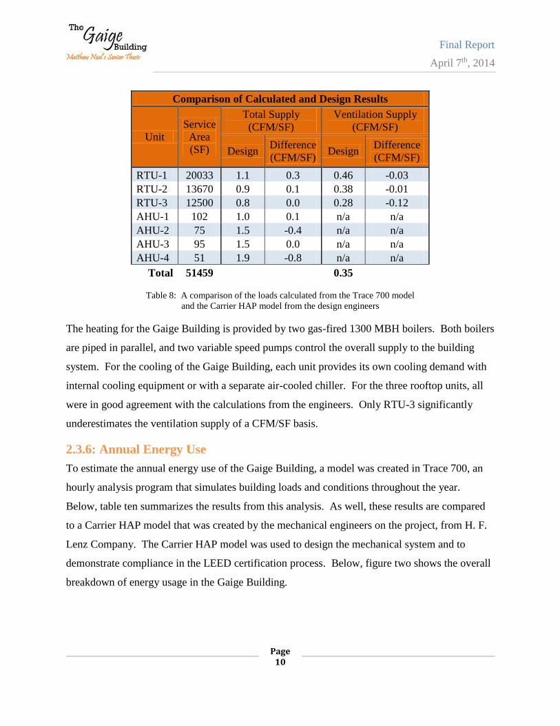
Comparison of Calculated and Design Results

Unit

Service

Area

(SF)

Total Supply

(CFM/SF)

Ventilation Supply

(CFM/SF)

Design Difference

(CFM/SF) Design

Difference

(CFM/SF)

RTU-1 20033 1.1 0.3 0.46 -0.03

RTU-2 13670 0.9 0.1 0.38 -0.01

RTU-3 12500 0.8 0.0 0.28 -0.12

AHU-1 102 1.0 0.1 n/a n/a

AHU-2 75 1.5 -0.4 n/a n/a

AHU-3 95 1.5 0.0 n/a n/a

AHU-4 51 1.9 -0.8 n/a n/a

Total 51459 0.35

Table 8: A comparison of the loads calculated from the Trace 700 model

and the Carrier HAP model from the design engineers

The heating for the Gaige Building is provided by two gas-fired 1300 MBH boilers. Both boilers

are piped in parallel, and two variable speed pumps control the overall supply to the building

system. For the cooling of the Gaige Building, each unit provides its own cooling demand with

internal cooling equipment or with a separate air-cooled chiller. For the three rooftop units, all

were in good agreement with the calculations from the engineers. Only RTU-3 significantly

underestimates the ventilation supply of a CFM/SF basis.

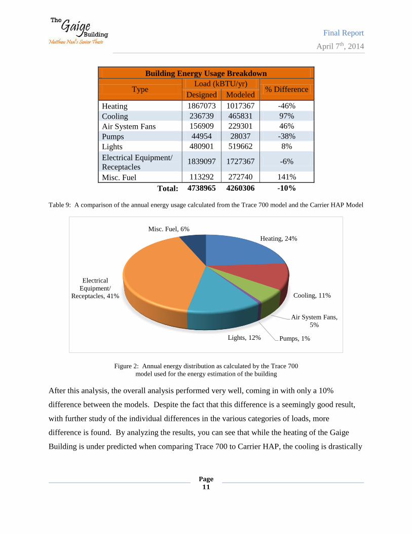
2.3.6: Annual Energy Use

To estimate the annual energy use of the Gaige Building, a model was created in Trace 700, an

hourly analysis program that simulates building loads and conditions throughout the year.

Below, table ten summarizes the results from this analysis. As well, these results are compared

to a Carrier HAP model that was created by the mechanical engineers on the project, from H. F.

Lenz Company. The Carrier HAP model was used to design the mechanical system and to

demonstrate compliance in the LEED certification process. Below, figure two shows the overall

breakdown of energy usage in the Gaige Building.

Final Report

April 7th, 2014

Page 11

Building Energy Usage Breakdown

Type Load (kBTU/yr)

% Difference Designed Modeled

Heating 1867073 1017367 -46%

Cooling 236739 465831 97%

Air System Fans 156909 229301 46%

Pumps 44954 28037 -38%

Lights 480901 519662 8%

Electrical Equipment/

Receptacles 1839097 1727367 -6%

Misc. Fuel 113292 272740 141%

Total: 4738965 4260306 -10%

Table 9: A comparison of the annual energy usage calculated from the Trace 700 model and the Carrier HAP Model

Figure 2: Annual energy distribution as calculated by the Trace 700

model used for the energy estimation of the building

After this analysis, the overall analysis performed very well, coming in with only a 10%

difference between the models. Despite the fact that this difference is a seemingly good result,

with further study of the individual differences in the various categories of loads, more

difference is found. By analyzing the results, you can see that while the heating of the Gaige

Building is under predicted when comparing Trace 700 to Carrier HAP, the cooling is drastically

Heating, 24%

Cooling, 11%

Air System Fans,

5%

Pumps, 1%Lights, 12%

Electrical

Equipment/

Receptacles, 41%

Misc. Fuel, 6%

Final Report

April 7th, 2014

Page 12

over predicted. These two errors will tend to cancel each other out, and hide some amount of

difference between the models.

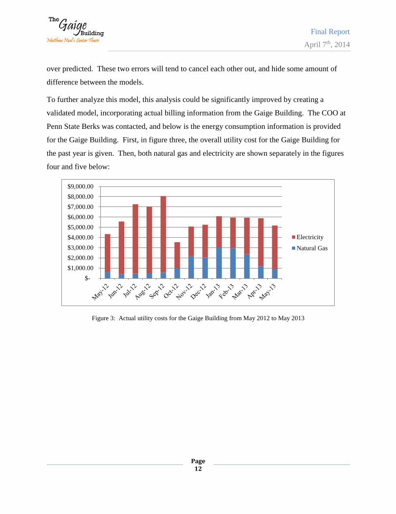
To further analyze this model, this analysis could be significantly improved by creating a

validated model, incorporating actual billing information from the Gaige Building. The COO at

Penn State Berks was contacted, and below is the energy consumption information is provided

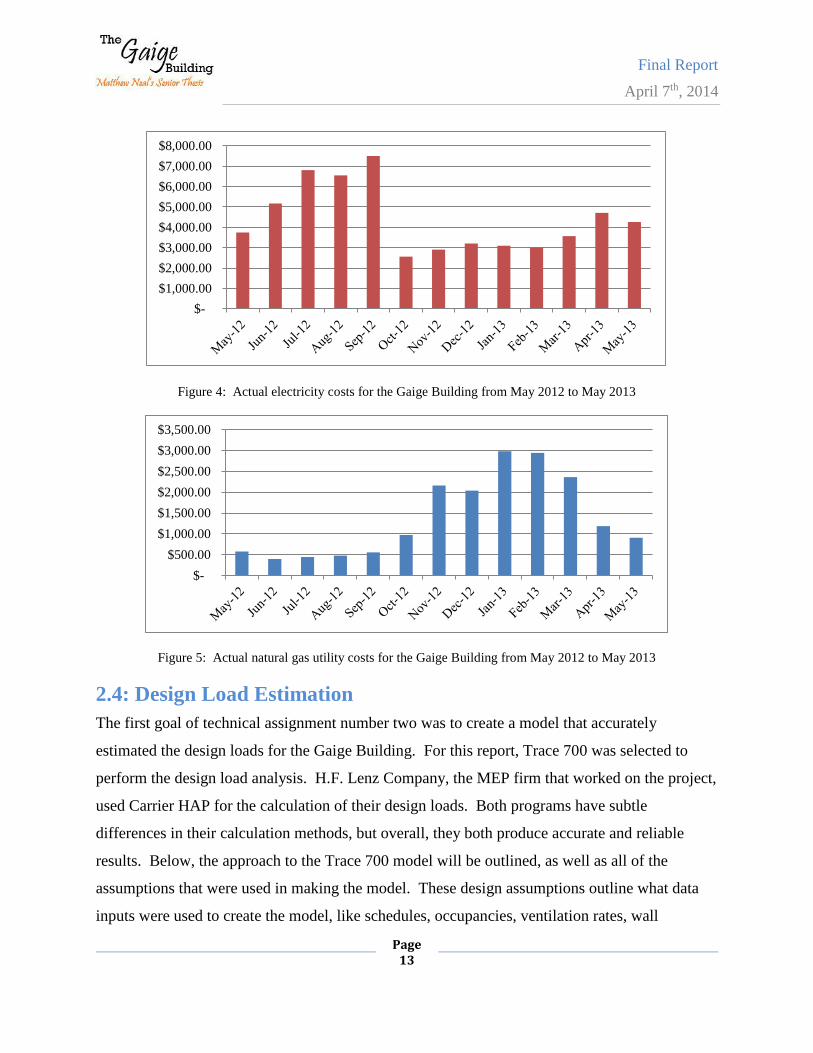
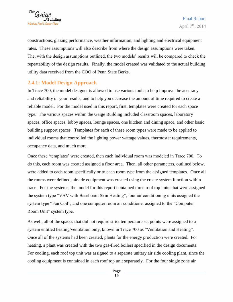
for the Gaige Building. First, in figure three, the overall utility cost for the Gaige Building for

the past year is given. Then, both natural gas and electricity are shown separately in the figures

four and five below:

Figure 3: Actual utility costs for the Gaige Building from May 2012 to May 2013

$-

$1,000.00

$2,000.00

$3,000.00

$4,000.00

$5,000.00

$6,000.00

$7,000.00

$8,000.00

$9,000.00

Electricity

Natural Gas

Final Report

April 7th, 2014

Page 13

Figure 4: Actual electricity costs for the Gaige Building from May 2012 to May 2013

Figure 5: Actual natural gas utility costs for the Gaige Building from May 2012 to May 2013

2.4: Design Load Estimation

The first goal of technical assignment number two was to create a model that accurately

estimated the design loads for the Gaige Building. For this report, Trace 700 was selected to

perform the design load analysis. H.F. Lenz Company, the MEP firm that worked on the project,

used Carrier HAP for the calculation of their design loads. Both programs have subtle

differences in their calculation methods, but overall, they both produce accurate and reliable

results. Below, the approach to the Trace 700 model will be outlined, as well as all of the

assumptions that were used in making the model. These design assumptions outline what data

inputs were used to create the model, like schedules, occupancies, ventilation rates, wall

$-

$1,000.00

$2,000.00

$3,000.00

$4,000.00

$5,000.00

$6,000.00

$7,000.00

$8,000.00

$-

$500.00

$1,000.00

$1,500.00

$2,000.00

$2,500.00

$3,000.00

$3,500.00

Final Report

April 7th, 2014

Page 14

constructions, glazing performance, weather information, and lighting and electrical equipment

rates. These assumptions will also describe from where the design assumptions were taken.

The, with the design assumptions outlined, the two models’ results will be compared to check the

repeatability of the design results. Finally, the model created was validated to the actual building

utility data received from the COO of Penn State Berks.

2.4.1: Model Design Approach

In Trace 700, the model designer is allowed to use various tools to help improve the accuracy

and reliability of your results, and to help you decrease the amount of time required to create a

reliable model. For the model used in this report, first, templates were created for each space

type. The various spaces within the Gaige Building included classroom spaces, laboratory

spaces, office spaces, lobby spaces, lounge spaces, one kitchen and dining space, and other basic

building support spaces. Templates for each of these room types were made to be applied to

individual rooms that controlled the lighting power wattage values, thermostat requirements,

occupancy data, and much more.

Once these ‘templates’ were created, then each individual room was modeled in Trace 700. To

do this, each room was created assigned a floor area. Then, all other parameters, outlined below,

were added to each room specifically or to each room type from the assigned templates. Once all

the rooms were defined, airside equipment was created using the create system function within

trace. For the systems, the model for this report contained three roof top units that were assigned

the system type “VAV with Baseboard Skin Heating”, four air conditioning units assigned the

system type “Fan Coil”, and one computer room air conditioner assigned to the “Computer

Room Unit” system type.

As well, all of the spaces that did not require strict temperature set points were assigned to a

system entitled heating/ventilation only, known in Trace 700 as “Ventilation and Heating”.

Once all of the systems had been created, plants for the energy production were created. For

heating, a plant was created with the two gas-fired boilers specified in the design documents.

For cooling, each roof top unit was assigned to a separate unitary air side cooling plant, since the

cooling equipment is contained in each roof top unit separately. For the four single zone air

Final Report

April 7th, 2014

Page 15

conditioning units and the computer room air conditioner, each system was assigned to a

separate air-cooled chiller, each of which was found in the design documents as well. All

cooling equipment was assigned to the electric utility and heating was assigned to the gas utility.

2.4.2: System Design Assumptions

The following sections outline how the building was modeled, what data was used for the system

inputs as far as internal loads are concerned, and where the data was obtained from. Many of the

design assumptions were pulled directly from the model created by H.F. Lenz, for this report

aims to recreate accurately the actual model used to design the building. Despite the fact that

values were pulled from the model, it was always ensured that the values used in this model

accurately reflected the building’s design, and it will be discussed where variations between what

was designed and what was modeled in Carrier HAP were discovered, and how those variations

were addressed.

2.4.2.1: Design Condition Assumptions

For the Gaige Building, standard values were used for space thermostat set points. All occupied

spaces were set to values specified in table one below. This space type constitutes the majority

of the building, but spaces that only require heating and ventilation were designed at differing

thermostat set points. The set points for the Gaige building, and the chosen set points for this

model, can be seen previously in table three.

2.4.2.2: Occupancy Assumptions

For the Gaige Building, in order to recreate the best match between the model created by H.F.

Lenz Company and the model created for this report, values were chosen based upon the design

values found in both the design documentation of the Gaige Building and the model created by

H.F. Lenz Company. Although values could be calculated on an occupancy per 1000 SF basis

from ASHRAE recommendations, since design occupancies were available, they were used.

Final Report

April 7th, 2014

Page 16

2.4.2.3: Ventilation Assumptions

For the ventilation rates in the model, rates were obtained from the design documents from H.F.

Lenz Company. Although ventilation rates were calculated from the previous assignment,

technical report one, it is the goal of this assignment to best recreate a model for the building, as

designed. Because of this, the preloaded ASHRAE standards template values within Trace 700

were not used, and individual ventilation supply rates were input on a space by space basis.

2.4.2.4: Building Infiltration Assumptions

As per recommendation by the mechanical engineer from H.F. Lenz who worked on the project,

0.3 air changes per hour was used as the infiltration to all spaces within in the Gaige Building.

This value was selected based upon the fact that the Gaige Building is designed to be positively

pressurized, and it is of at least average construction quality. Since the building’s façade has

been given much thought, shown by its LEED Silver status, the building could probably be

considered of a higher quality construction, and a lower value for infiltration could have been

used. Since 0.3 air changes per hour was used in H.F. Lenz’s model in Carrier HAP, that value

was also adopted for the Trace 700 model created for this report.

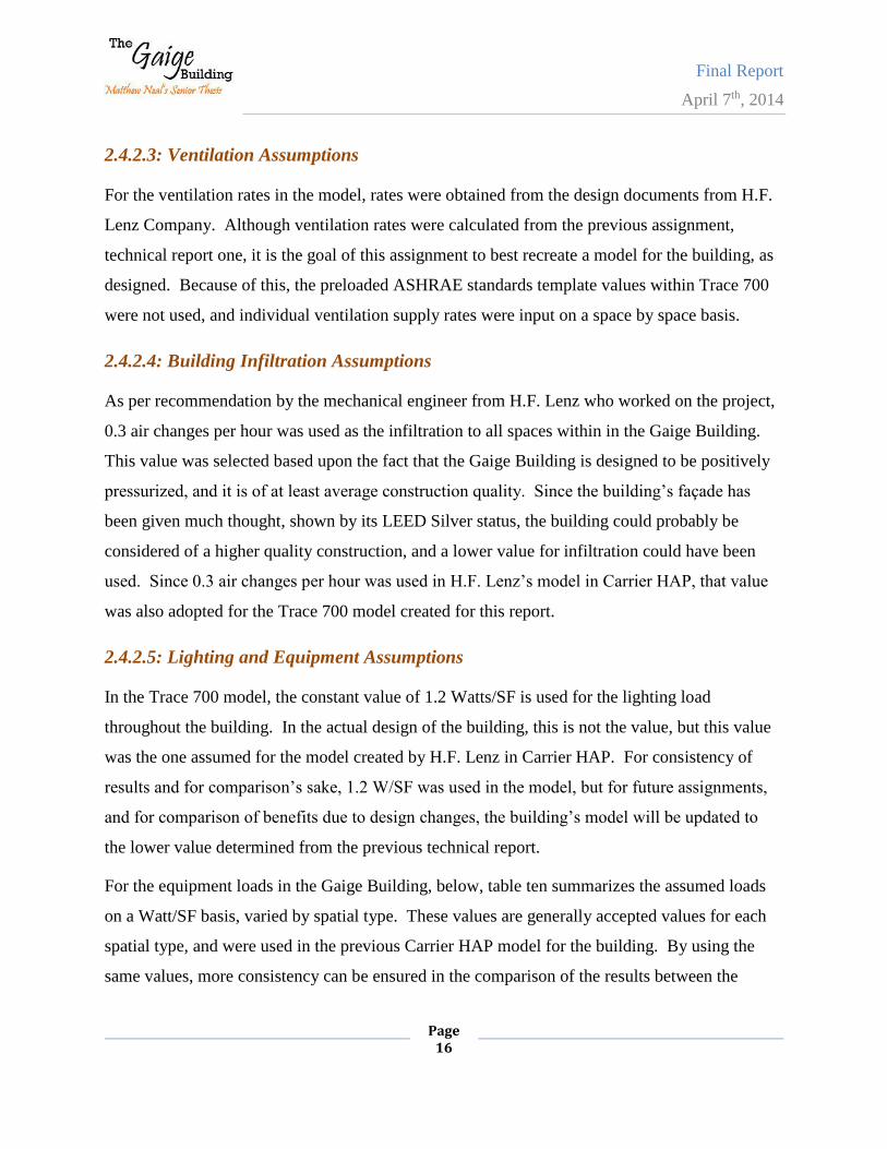
2.4.2.5: Lighting and Equipment Assumptions

In the Trace 700 model, the constant value of 1.2 Watts/SF is used for the lighting load

throughout the building. In the actual design of the building, this is not the value, but this value

was the one assumed for the model created by H.F. Lenz in Carrier HAP. For consistency of

results and for comparison’s sake, 1.2 W/SF was used in the model, but for future assignments,

and for comparison of benefits due to design changes, the building’s model will be updated to

the lower value determined from the previous technical report.

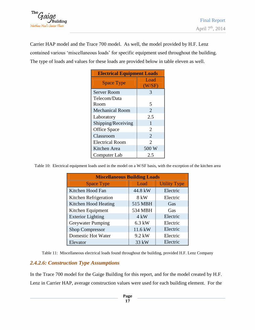
For the equipment loads in the Gaige Building, below, table ten summarizes the assumed loads

on a Watt/SF basis, varied by spatial type. These values are generally accepted values for each

spatial type, and were used in the previous Carrier HAP model for the building. By using the

same values, more consistency can be ensured in the comparison of the results between the

Final Report

April 7th, 2014

Page 17

Carrier HAP model and the Trace 700 model. As well, the model provided by H.F. Lenz

contained various ‘miscellaneous loads’ for specific equipment used throughout the building.

The type of loads and values for these loads are provided below in table eleven as well.

Electrical Equipment Loads

Space Type Load

(W/SF)

Server Room 3

Telecom/Data

Room 5

Mechanical Room 2

Laboratory 2.5

Shipping/Receiving 1

Office Space 2

Classroom 2

Electrical Room 2

Kitchen Area 500 W

Computer Lab 2.5

Table 10: Electrical equipment loads used in the model on a W/SF basis, with the exception of the kitchen area

Miscellaneous Building Loads

Space Type Load Utility Type

Kitchen Hood Fan 44.8 kW Electric

Kitchen Refrigeration 8 kW Electric

Kitchen Hood Heating 515 MBH Gas

Kitchen Equipment 534 MBH Gas

Exterior Lighting 4 kW Electric

Greywater Pumping 6.3 kW Electric

Shop Compressor 11.6 kW Electric

Domestic Hot Water 9.2 kW Electric

Elevator 33 kW Electric

Table 11: Miscellaneous electrical loads found throughout the building, provided H.F. Lenz Company

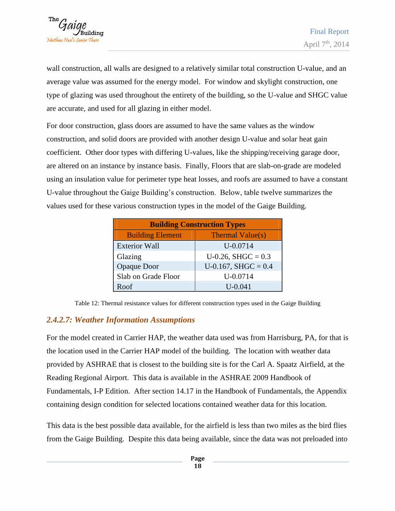
2.4.2.6: Construction Type Assumptions

In the Trace 700 model for the Gaige Building for this report, and for the model created by H.F.

Lenz in Carrier HAP, average construction values were used for each building element. For the

Final Report

April 7th, 2014

Page 18

wall construction, all walls are designed to a relatively similar total construction U-value, and an

average value was assumed for the energy model. For window and skylight construction, one

type of glazing was used throughout the entirety of the building, so the U-value and SHGC value

are accurate, and used for all glazing in either model.

For door construction, glass doors are assumed to have the same values as the window

construction, and solid doors are provided with another design U-value and solar heat gain

coefficient. Other door types with differing U-values, like the shipping/receiving garage door,

are altered on an instance by instance basis. Finally, Floors that are slab-on-grade are modeled

using an insulation value for perimeter type heat losses, and roofs are assumed to have a constant

U-value throughout the Gaige Building’s construction. Below, table twelve summarizes the

values used for these various construction types in the model of the Gaige Building.

Building Construction Types

Building Element Thermal Value(s)

Exterior Wall U-0.0714

Glazing U-0.26, SHGC = 0.3

Opaque Door U-0.167, SHGC = 0.4

Slab on Grade Floor U-0.0714

Roof U-0.041

Table 12: Thermal resistance values for different construction types used in the Gaige Building

2.4.2.7: Weather Information Assumptions

For the model created in Carrier HAP, the weather data used was from Harrisburg, PA, for that is

the location used in the Carrier HAP model of the building. The location with weather data

provided by ASHRAE that is closest to the building site is for the Carl A. Spaatz Airfield, at the

Reading Regional Airport. This data is available in the ASHRAE 2009 Handbook of

Fundamentals, I-P Edition. After section 14.17 in the Handbook of Fundamentals, the Appendix

containing design condition for selected locations contained weather data for this location.

This data is the best possible data available, for the airfield is less than two miles as the bird flies

from the Gaige Building. Despite this data being available, since the data was not preloaded into

Final Report

April 7th, 2014

Page 19

Carrier HAP, Harrisburg, PA was used for the previous design of the building by H.F. Lenz. For

my future models, the design overrides option in Trace 700 will be used to specify the design

criterion used for the Gaige Building. The data used in the following mechanical depth analysis

incorporated the weather data for Spaatz Airfield, show previously in table three.

2.4.2.8: Schedule Assumptions

When the original model of the Gaige Building was created by H.F. Lenz, various custom

schedules were made for use in the Carrier HAP model. Schedules that were assigned are

provided in Appendix B. The schedules given for nighttime, compressor, greywater pumping,

and kitchen hoods are all used for the miscellaneous loads specified in the Carrier HAP model

for the Gaige Building. These are utilization schedules that control the operation of the

equipment. Other than that, the “All-Classroom” schedule is the main schedule used for the

Gaige Building for the operation of all people, lighting, and ventilation, apart from a separate

people and lighting schedule provided for the Office Spaces. As well, and Office miscellaneous

load schedule is provided for office equipment operation. Again, all of these schedules can be

seen in Appendix B of this report.

2.4.3: Model Comparison with Utility Data

Once this new data was obtained, first, new cost factors were input into the previous Trace 700

model. The new natural gas and electricity costs were taken to be the average of the costs from

the past year of data, and then the annual energy costs were estimated. Below, in table nineteen,

the modeled results with the updated utility costs are compared to the actual charges from the

Gaige building bills from June 2012 to May 2013.

Final Report

April 7th, 2014

Page 20

Annual Energy Cost Information

Modeled (Trace 700)

Natural Gas $ 23,396.00

Electricity $ 85,404.00

Actual Cost from Billing

Natural Gas $ 17,431.31

Electricity $ 53,390.19

Table 13: Annual energy costs for both the Trace 700 model and actual data from the Gaige Building

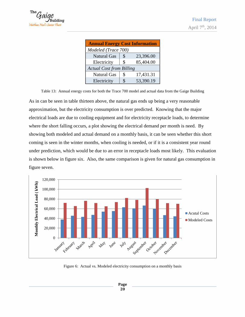
As in can be seen in table thirteen above, the natural gas ends up being a very reasonable

approximation, but the electricity consumption is over predicted. Knowing that the major

electrical loads are due to cooling equipment and for electricity receptacle loads, to determine

where the short falling occurs, a plot showing the electrical demand per month is need. By

showing both modeled and actual demand on a monthly basis, it can be seen whether this short

coming is seen in the winter months, when cooling is needed, or if it is a consistent year round

under prediction, which would be due to an error in receptacle loads most likely. This evaluation

is shown below in figure six. Also, the same comparison is given for natural gas consumption in

figure seven.

Figure 6: Actual vs. Modeled electricity consumption on a monthly basis

0

20,000

40,000

60,000

80,000

100,000

120,000

Mo

nth

ly E

lect

rica

l L

oa

d (

kW

h)

Acutal Costs

Modeled Costs

Final Report

April 7th, 2014

Page 21

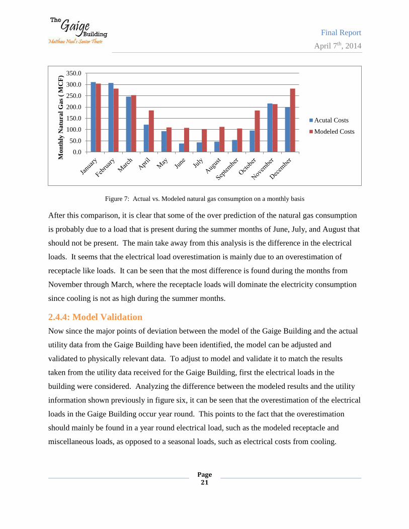
Figure 7: Actual vs. Modeled natural gas consumption on a monthly basis

After this comparison, it is clear that some of the over prediction of the natural gas consumption

is probably due to a load that is present during the summer months of June, July, and August that

should not be present. The main take away from this analysis is the difference in the electrical

loads. It seems that the electrical load overestimation is mainly due to an overestimation of

receptacle like loads. It can be seen that the most difference is found during the months from

November through March, where the receptacle loads will dominate the electricity consumption

since cooling is not as high during the summer months.

2.4.4: Model Validation

Now since the major points of deviation between the model of the Gaige Building and the actual

utility data from the Gaige Building have been identified, the model can be adjusted and

validated to physically relevant data. To adjust to model and validate it to match the results

taken from the utility data received for the Gaige Building, first the electrical loads in the

building were considered. Analyzing the difference between the modeled results and the utility

information shown previously in figure six, it can be seen that the overestimation of the electrical

loads in the Gaige Building occur year round. This points to the fact that the overestimation

should mainly be found in a year round electrical load, such as the modeled receptacle and

miscellaneous loads, as opposed to a seasonal loads, such as electrical costs from cooling.

0.0

50.0

100.0

150.0

200.0

250.0

300.0

350.0

Mo

nth

ly N

atu

ral

Ga

s (

MC

F)

Acutal Costs

Modeled Costs

Final Report

April 7th, 2014

Page 22

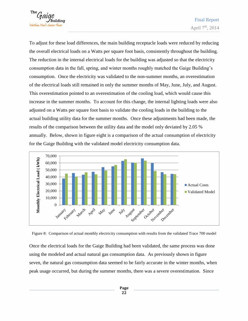
To adjust for these load differences, the main building receptacle loads were reduced by reducing

the overall electrical loads on a Watts per square foot basis, consistently throughout the building.

The reduction in the internal electrical loads for the building was adjusted so that the electricity

consumption data in the fall, spring, and winter months roughly matched the Gaige Building’s

consumption. Once the electricity was validated to the non-summer months, an overestimation

of the electrical loads still remained in only the summer months of May, June, July, and August.

This overestimation pointed to an overestimation of the cooling load, which would cause this

increase in the summer months. To account for this change, the internal lighting loads were also

adjusted on a Watts per square foot basis to validate the cooling loads in the building to the

actual building utility data for the summer months. Once these adjustments had been made, the

results of the comparison between the utility data and the model only deviated by 2.05 %

annually. Below, shown in figure eight is a comparison of the actual consumption of electricity

for the Gaige Building with the validated model electricity consumption data.

Figure 8: Comparison of actual monthly electricity consumption with results from the validated Trace 700 model

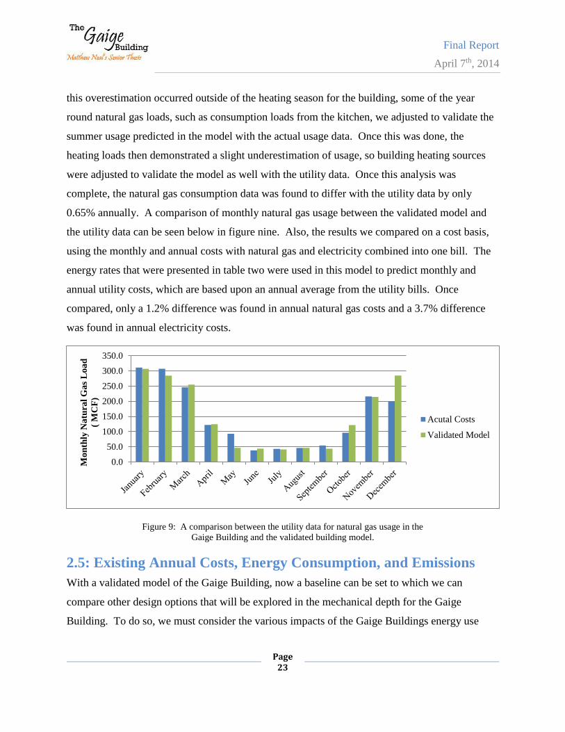
Once the electrical loads for the Gaige Building had been validated, the same process was done

using the modeled and actual natural gas consumption data. As previously shown in figure

seven, the natural gas consumption data seemed to be fairly accurate in the winter months, when

peak usage occurred, but during the summer months, there was a severe overestimation. Since

0

10,000

20,000

30,000

40,000

50,000

60,000

70,000

Mo

nth

ly E

lect

rica

l L

oa

d (

kW

h)

Actual Costs

Validated Model

Final Report

April 7th, 2014

Page 23

this overestimation occurred outside of the heating season for the building, some of the year

round natural gas loads, such as consumption loads from the kitchen, we adjusted to validate the

summer usage predicted in the model with the actual usage data. Once this was done, the

heating loads then demonstrated a slight underestimation of usage, so building heating sources

were adjusted to validate the model as well with the utility data. Once this analysis was

complete, the natural gas consumption data was found to differ with the utility data by only

0.65% annually. A comparison of monthly natural gas usage between the validated model and

the utility data can be seen below in figure nine. Also, the results we compared on a cost basis,

using the monthly and annual costs with natural gas and electricity combined into one bill. The

energy rates that were presented in table two were used in this model to predict monthly and

annual utility costs, which are based upon an annual average from the utility bills. Once

compared, only a 1.2% difference was found in annual natural gas costs and a 3.7% difference

was found in annual electricity costs.

Figure 9: A comparison between the utility data for natural gas usage in the

Gaige Building and the validated building model.

2.5: Existing Annual Costs, Energy Consumption, and Emissions

With a validated model of the Gaige Building, now a baseline can be set to which we can

compare other design options that will be explored in the mechanical depth for the Gaige

Building. To do so, we must consider the various impacts of the Gaige Buildings energy use

0.0

50.0

100.0

150.0

200.0

250.0

300.0

350.0

Mo

nth

ly N

atu

ral

Ga

s L

oa

d

( M

CF

)

Acutal Costs

Validated Model

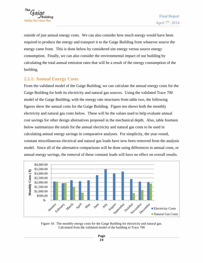
Final Report

April 7th, 2014

Page 24

outside of just annual energy costs. We can also consider how much energy would have been

required to produce the energy and transport it to the Gaige Building from whatever source the

energy came from. This is done below by considered site energy versus source energy

consumption. Finally, we can also consider the environmental impact of our building by

calculating the total annual emission rates that will be a result of the energy consumption of the

building.

2.5.1: Annual Energy Costs

From the validated model of the Gaige Building, we can calculate the annual energy costs for the

Gaige Building for both its electricity and natural gas sources. Using the validated Trace 700

model of the Gaige Building, with the energy rate structures from table two, the following

figures show the annual costs for the Gaige Building. Figure ten shows both the monthly

electricity and natural gas costs below. These will be the values used to help evaluate annual

cost savings for other design alternatives proposed in the mechanical depth. Also, table fourteen

below summarizes the totals for the annual electricity and natural gas costs to be used in

calculating annual energy savings in comparative analyses. For simplicity, the year-round,

constant miscellaneous electrical and natural gas loads have now been removed from the analysis

model. Since all of the alternative comparisons will be done using differences in annual costs, or

annual energy savings, the removal of these constant loads will have no effect on overall results.

Figure 10: The monthly energy costs for the Gaige Building for electricity and natural gas.

Calculated from the validated model of the building in Trace 700

$-

$500.00

$1,000.00

$1,500.00

$2,000.00

$2,500.00

$3,000.00

$3,500.00

$4,000.00

Mo

nth

ly C

ost

s (

$)

Electricity Costs

Natural Gas Costs

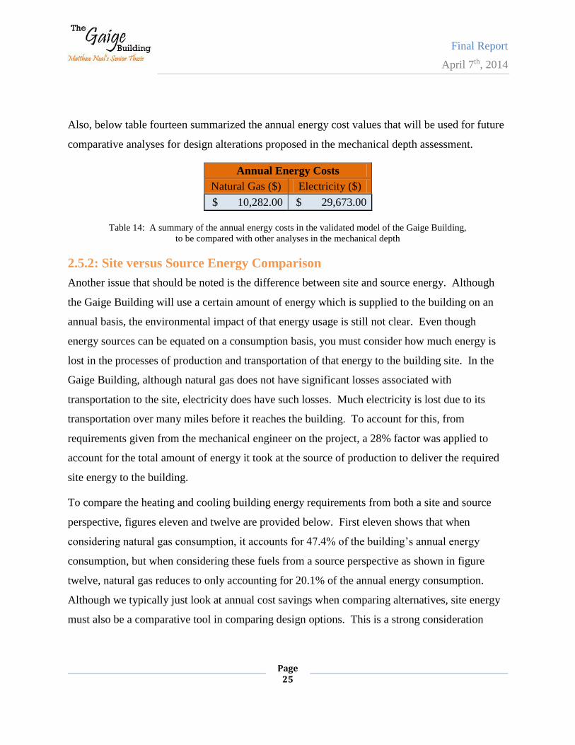
Final Report

April 7th, 2014

Page 25

Also, below table fourteen summarized the annual energy cost values that will be used for future

comparative analyses for design alterations proposed in the mechanical depth assessment.

Annual Energy Costs

Natural Gas ($) Electricity ($)

$ 10,282.00 $ 29,673.00

Table 14: A summary of the annual energy costs in the validated model of the Gaige Building,

to be compared with other analyses in the mechanical depth

2.5.2: Site versus Source Energy Comparison

Another issue that should be noted is the difference between site and source energy. Although

the Gaige Building will use a certain amount of energy which is supplied to the building on an

annual basis, the environmental impact of that energy usage is still not clear. Even though

energy sources can be equated on a consumption basis, you must consider how much energy is

lost in the processes of production and transportation of that energy to the building site. In the

Gaige Building, although natural gas does not have significant losses associated with

transportation to the site, electricity does have such losses. Much electricity is lost due to its

transportation over many miles before it reaches the building. To account for this, from

requirements given from the mechanical engineer on the project, a 28% factor was applied to

account for the total amount of energy it took at the source of production to deliver the required

site energy to the building.

To compare the heating and cooling building energy requirements from both a site and source

perspective, figures eleven and twelve are provided below. First eleven shows that when

considering natural gas consumption, it accounts for 47.4% of the building’s annual energy

consumption, but when considering these fuels from a source perspective as shown in figure

twelve, natural gas reduces to only accounting for 20.1% of the annual energy consumption.

Although we typically just look at annual cost savings when comparing alternatives, site energy

must also be a comparative tool in comparing design options. This is a strong consideration

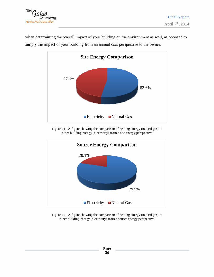
Final Report

April 7th, 2014

Page 26

when determining the overall impact of your building on the environment as well, as opposed to

simply the impact of your building from an annual cost perspective to the owner.

Figure 11: A figure showing the comparison of heating energy (natural gas) to

other building energy (electricity) from a site energy perspective

Figure 12: A figure showing the comparison of heating energy (natural gas) to

other building energy (electricity) from a source energy perspective

52.6%

47.4%

Site Energy Comparison

Electricity Natural Gas

79.9%

20.1%

Source Energy Comparison


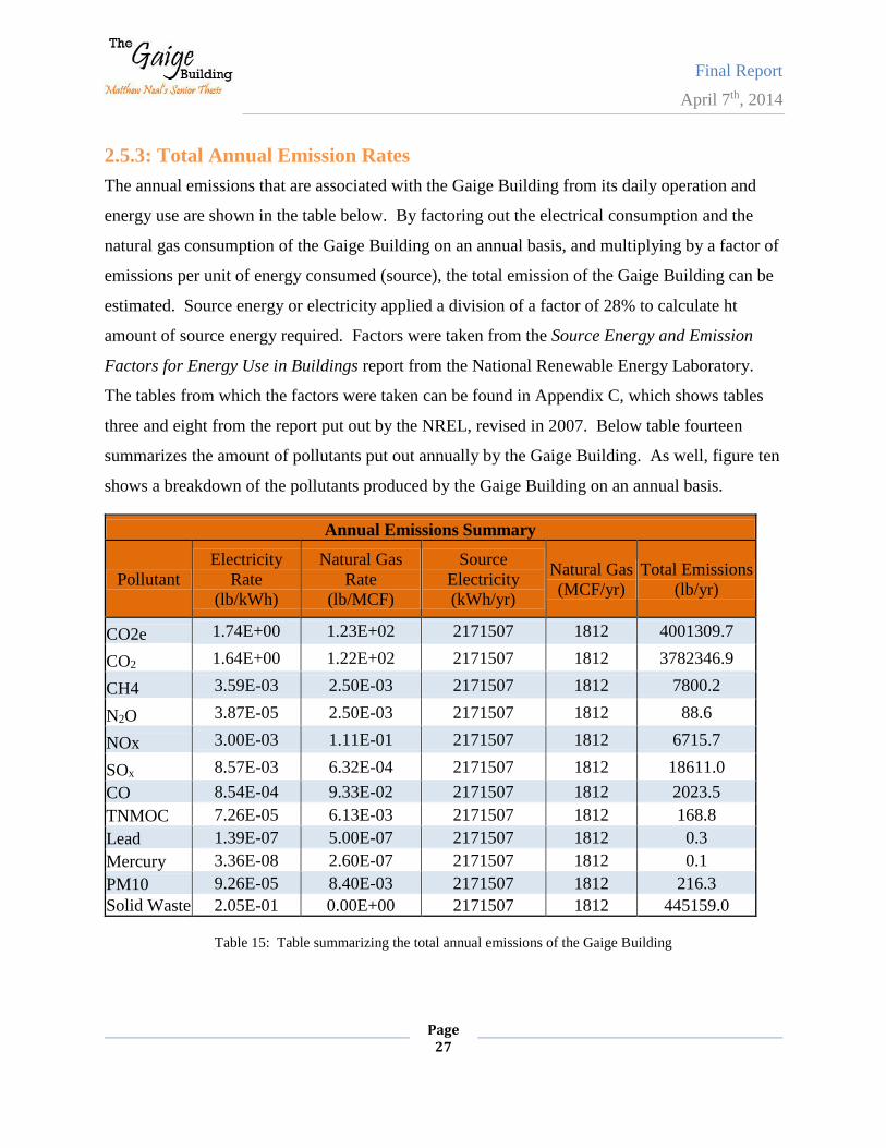
Final Report

April 7th, 2014

Page 27

2.5.3: Total Annual Emission Rates

The annual emissions that are associated with the Gaige Building from its daily operation and

energy use are shown in the table below. By factoring out the electrical consumption and the

natural gas consumption of the Gaige Building on an annual basis, and multiplying by a factor of

emissions per unit of energy consumed (source), the total emission of the Gaige Building can be

estimated. Source energy or electricity applied a division of a factor of 28% to calculate ht

amount of source energy required. Factors were taken from the Source Energy and Emission

Factors for Energy Use in Buildings report from the National Renewable Energy Laboratory.

The tables from which the factors were taken can be found in Appendix C, which shows tables

three and eight from the report put out by the NREL, revised in 2007. Below table fourteen

summarizes the amount of pollutants put out annually by the Gaige Building. As well, figure ten

shows a breakdown of the pollutants produced by the Gaige Building on an annual basis.

Annual Emissions Summary

Pollutant

Electricity

Rate

(lb/kWh)

Natural Gas

Rate

(lb/MCF)

Source

Electricity

(kWh/yr)

Natural Gas

(MCF/yr)

Total Emissions

(lb/yr)

CO2e 1.74E+00 1.23E+02 2171507 1812 4001309.7

CO2 1.64E+00 1.22E+02 2171507 1812 3782346.9

CH4 3.59E-03 2.50E-03 2171507 1812 7800.2

N2O 3.87E-05 2.50E-03 2171507 1812 88.6

NOx 3.00E-03 1.11E-01 2171507 1812 6715.7

SOx 8.57E-03 6.32E-04 2171507 1812 18611.0

CO 8.54E-04 9.33E-02 2171507 1812 2023.5

TNMOC 7.26E-05 6.13E-03 2171507 1812 168.8

Lead 1.39E-07 5.00E-07 2171507 1812 0.3

Mercury 3.36E-08 2.60E-07 2171507 1812 0.1

PM10 9.26E-05 8.40E-03 2171507 1812 216.3

Solid Waste 2.05E-01 0.00E+00 2171507 1812 445159.0

Table 15: Table summarizing the total annual emissions of the Gaige Building

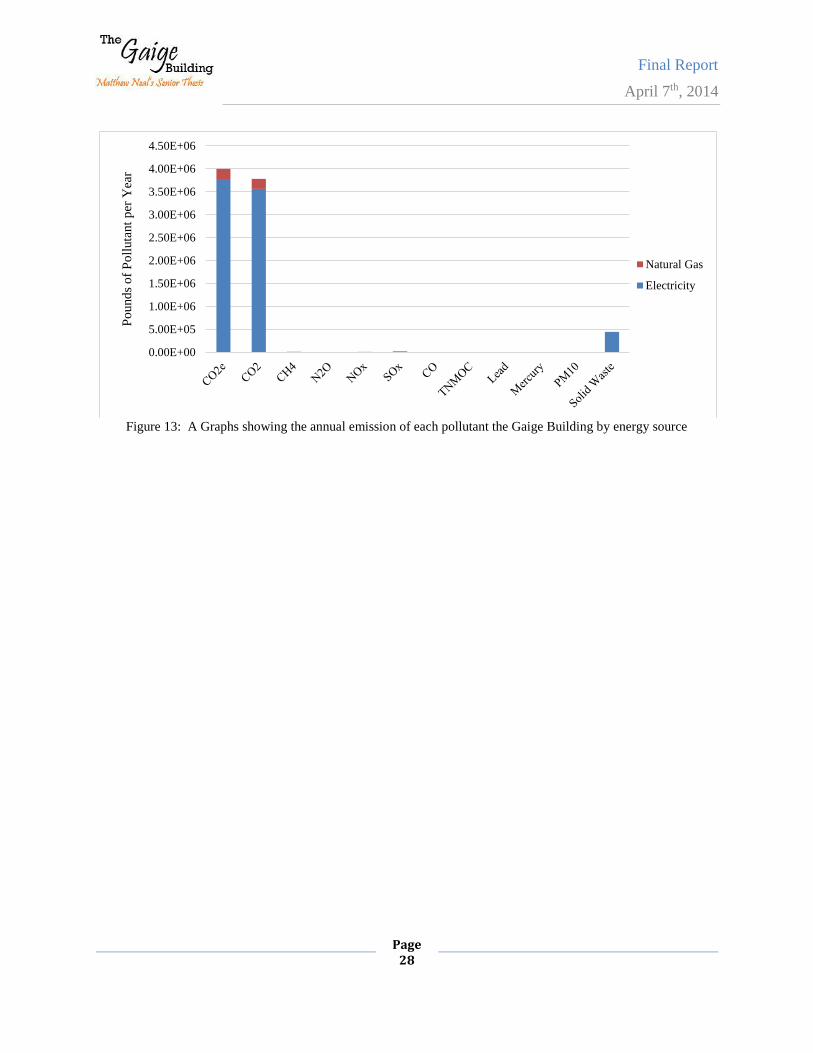
Final Report

April 7th, 2014

Page 28

Figure 13: A Graphs showing the annual emission of each pollutant the Gaige Building by energy source

0.00E+00

5.00E+05

1.00E+06

1.50E+06

2.00E+06

2.50E+06

3.00E+06

3.50E+06

4.00E+06

4.50E+06

Po

und

s o

f P

oll

uta

nt

per

Yea

r

Natural Gas

Electricity

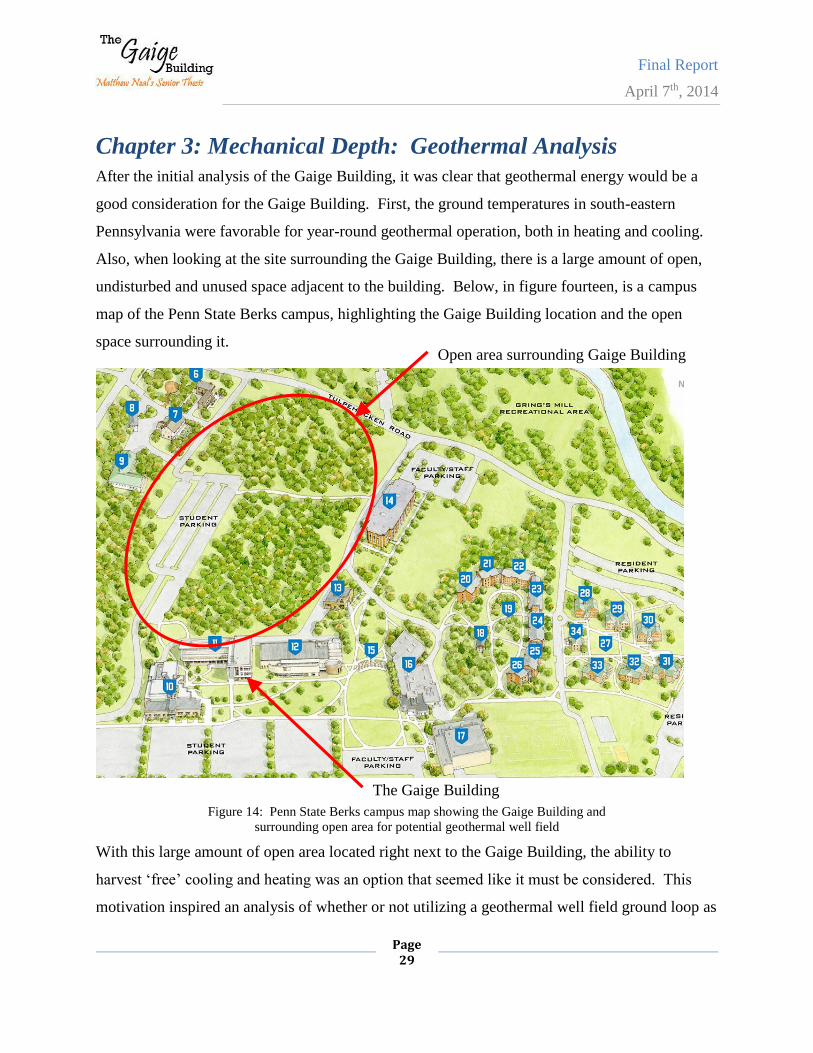
Final Report

April 7th, 2014

Page 29

Chapter 3: Mechanical Depth: Geothermal Analysis

After the initial analysis of the Gaige Building, it was clear that geothermal energy would be a

good consideration for the Gaige Building. First, the ground temperatures in south-eastern

Pennsylvania were favorable for year-round geothermal operation, both in heating and cooling.

Also, when looking at the site surrounding the Gaige Building, there is a large amount of open,

undisturbed and unused space adjacent to the building. Below, in figure fourteen, is a campus

map of the Penn State Berks campus, highlighting the Gaige Building location and the open

space surrounding it.

Figure 14: Penn State Berks campus map showing the Gaige Building and

surrounding open area for potential geothermal well field

With this large amount of open area located right next to the Gaige Building, the ability to

harvest ‘free’ cooling and heating was an option that seemed like it must be considered. This

motivation inspired an analysis of whether or not utilizing a geothermal well field ground loop as

Open area surrounding Gaige Building

The Gaige Building

Final Report

April 7th, 2014

Page 30

an energy source for the Gaige Building would decrease the annual energy costs enough to

justify the initial increase in first costs required for the well field.

Out of this study, it was also realized that the open space available was much larger than was

needed for a geothermal well field for just the Gaige Building. With this, a second mechanical

study was conducted, to determine if it would be feasible to construct a centralized geothermal

well field to serve the majority of the campus buildings. With the large amount of space

available, and with a large collections of building near each other, all under the same owner,

much more annual savings could be realized when considering the larger campus that the Gaige

Building was located in. To study this option, models of the campus as a whole were created,

and initial first cost increases were compared against annual savings to help determine if the

large first costs of a campus wide geothermal system would pay off over the life of the system.

3.1 Geothermal Analysis of the Gaige Building

First, an analysis of the Gaige Building’s potential for a geothermal well-field system was

analyzed. In the sections below, an overview will be given of the design objectives for this

system, the overall configuration of the system, and the layout and setup of the geothermal well

field. Then, alterations in the Gaige Building’s internal systems layout will be discussed.

Finally, annual savings from the geothermal system will be modeled and calculated, and the

performance of the new system will be evaluated upon its overall emissions reductions and the

payback period for the system using a discounted payback life-cycle cost analysis.

3.1.1: Design Objectives

For the Gaige Building the system design objects were straightforward: reduce annual emissions

and utility costs by utilizing the thermal energy located onsite. In a geothermal system, the

fundamental reason it works is due to the relatively constant ground temperatures that can be

found when you are only 10 to 20 feet below ground level. Despite the large temperature

fluctuations that we experience above ground, ranging from 0⁰ up to 90⁰ during normal yearly

conditions, the ground temperature remains relatively constant. With this, during the summer

months, when cooling is needed, the ground can act as a heat sink. Water source heat pumps can

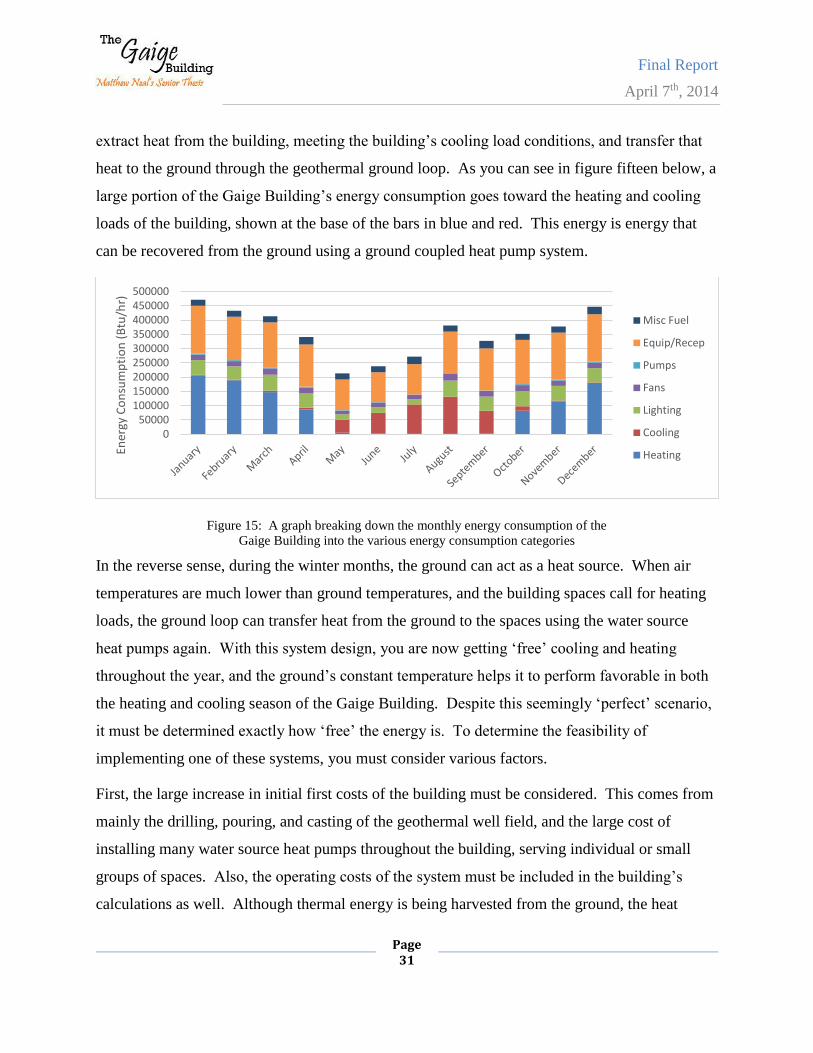
Final Report

April 7th, 2014

Page 31

extract heat from the building, meeting the building’s cooling load conditions, and transfer that

heat to the ground through the geothermal ground loop. As you can see in figure fifteen below, a

large portion of the Gaige Building’s energy consumption goes toward the heating and cooling

loads of the building, shown at the base of the bars in blue and red. This energy is energy that

can be recovered from the ground using a ground coupled heat pump system.

Figure 15: A graph breaking down the monthly energy consumption of the

Gaige Building into the various energy consumption categories

In the reverse sense, during the winter months, the ground can act as a heat source. When air

temperatures are much lower than ground temperatures, and the building spaces call for heating

loads, the ground loop can transfer heat from the ground to the spaces using the water source

heat pumps again. With this system design, you are now getting ‘free’ cooling and heating

throughout the year, and the ground’s constant temperature helps it to perform favorable in both

the heating and cooling season of the Gaige Building. Despite this seemingly ‘perfect’ scenario,

it must be determined exactly how ‘free’ the energy is. To determine the feasibility of

implementing one of these systems, you must consider various factors.

First, the large increase in initial first costs of the building must be considered. This comes from

mainly the drilling, pouring, and casting of the geothermal well field, and the large cost of

installing many water source heat pumps throughout the building, serving individual or small

groups of spaces. Also, the operating costs of the system must be included in the building’s

calculations as well. Although thermal energy is being harvested from the ground, the heat

050000

100000150000200000250000300000350000400000450000500000

Ener

gy C

on

sum

pti

on

(B

tu/h

r)

Misc Fuel

Equip/Recep

Pumps

Fans

Lighting

Cooling

Heating

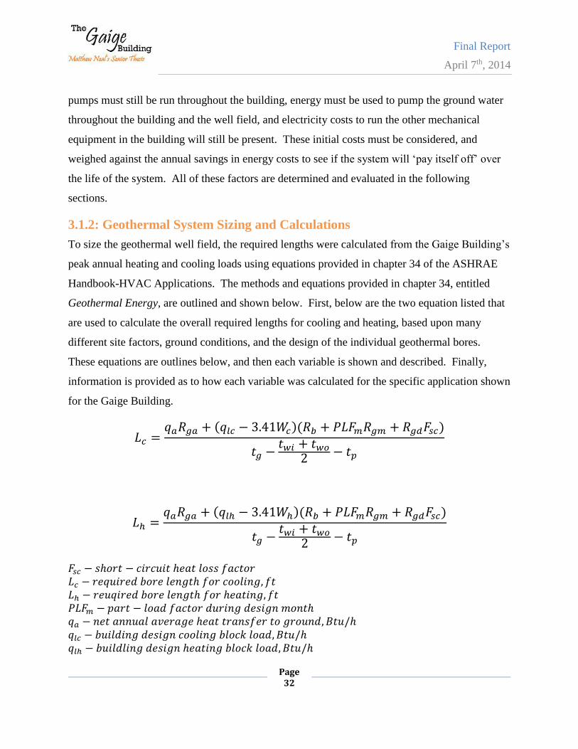
Final Report

April 7th, 2014

Page 32

pumps must still be run throughout the building, energy must be used to pump the ground water

throughout the building and the well field, and electricity costs to run the other mechanical

equipment in the building will still be present. These initial costs must be considered, and

weighed against the annual savings in energy costs to see if the system will ‘pay itself off’ over

the life of the system. All of these factors are determined and evaluated in the following

sections.

3.1.2: Geothermal System Sizing and Calculations

To size the geothermal well field, the required lengths were calculated from the Gaige Building’s

peak annual heating and cooling loads using equations provided in chapter 34 of the ASHRAE

Handbook-HVAC Applications. The methods and equations provided in chapter 34, entitled

Geothermal Energy, are outlined and shown below. First, below are the two equation listed that

are used to calculate the overall required lengths for cooling and heating, based upon many

different site factors, ground conditions, and the design of the individual geothermal bores.

These equations are outlines below, and then each variable is shown and described. Finally,

information is provided as to how each variable was calculated for the specific application shown

for the Gaige Building.

𝐿𝑐 =𝑞𝑎𝑅𝑔𝑎 + (𝑞𝑙𝑐 − 3.41𝑊𝑐)(𝑅𝑏 + 𝑃𝐿𝐹𝑚𝑅𝑔𝑚 + 𝑅𝑔𝑑𝐹𝑠𝑐)

𝑡𝑔 −𝑡𝑤𝑖 + 𝑡𝑤𝑜

2− 𝑡𝑝

𝐿ℎ =𝑞𝑎𝑅𝑔𝑎 + (𝑞𝑙ℎ − 3.41𝑊ℎ)(𝑅𝑏 + 𝑃𝐿𝐹𝑚𝑅𝑔𝑚 + 𝑅𝑔𝑑𝐹𝑠𝑐)

𝑡𝑔 −𝑡𝑤𝑖 + 𝑡𝑤𝑜

2− 𝑡𝑝

𝐹𝑠𝑐 − 𝑠ℎ𝑜𝑟𝑡 − 𝑐𝑖𝑟𝑐𝑢𝑖𝑡 ℎ𝑒𝑎𝑡 𝑙𝑜𝑠𝑠 𝑓𝑎𝑐𝑡𝑜𝑟

𝐿𝑐 − 𝑟𝑒𝑞𝑢𝑖𝑟𝑒𝑑 𝑏𝑜𝑟𝑒 𝑙𝑒𝑛𝑔𝑡ℎ 𝑓𝑜𝑟 𝑐𝑜𝑜𝑙𝑖𝑛𝑔, 𝑓𝑡

𝐿ℎ − 𝑟𝑒𝑢𝑞𝑖𝑟𝑒𝑑 𝑏𝑜𝑟𝑒 𝑙𝑒𝑛𝑔𝑡ℎ 𝑓𝑜𝑟 ℎ𝑒𝑎𝑡𝑖𝑛𝑔, 𝑓𝑡

𝑃𝐿𝐹𝑚 − 𝑝𝑎𝑟𝑡 − 𝑙𝑜𝑎𝑑 𝑓𝑎𝑐𝑡𝑜𝑟 𝑑𝑢𝑟𝑖𝑛𝑔 𝑑𝑒𝑠𝑖𝑔𝑛 𝑚𝑜𝑛𝑡ℎ

𝑞𝑎 − 𝑛𝑒𝑡 𝑎𝑛𝑛𝑢𝑎𝑙 𝑎𝑣𝑒𝑟𝑎𝑔𝑒 ℎ𝑒𝑎𝑡 𝑡𝑟𝑎𝑛𝑠𝑓𝑒𝑟 𝑡𝑜 𝑔𝑟𝑜𝑢𝑛𝑑, 𝐵𝑡𝑢/ℎ

𝑞𝑙𝑐 − 𝑏𝑢𝑖𝑙𝑑𝑖𝑛𝑔 𝑑𝑒𝑠𝑖𝑔𝑛 𝑐𝑜𝑜𝑙𝑖𝑛𝑔 𝑏𝑙𝑜𝑐𝑘 𝑙𝑜𝑎𝑑, 𝐵𝑡𝑢/ℎ

𝑞𝑙ℎ − 𝑏𝑢𝑖𝑙𝑑𝑙𝑖𝑛𝑔 𝑑𝑒𝑠𝑖𝑔𝑛 ℎ𝑒𝑎𝑡𝑖𝑛𝑔 𝑏𝑙𝑜𝑐𝑘 𝑙𝑜𝑎𝑑, 𝐵𝑡𝑢/ℎ

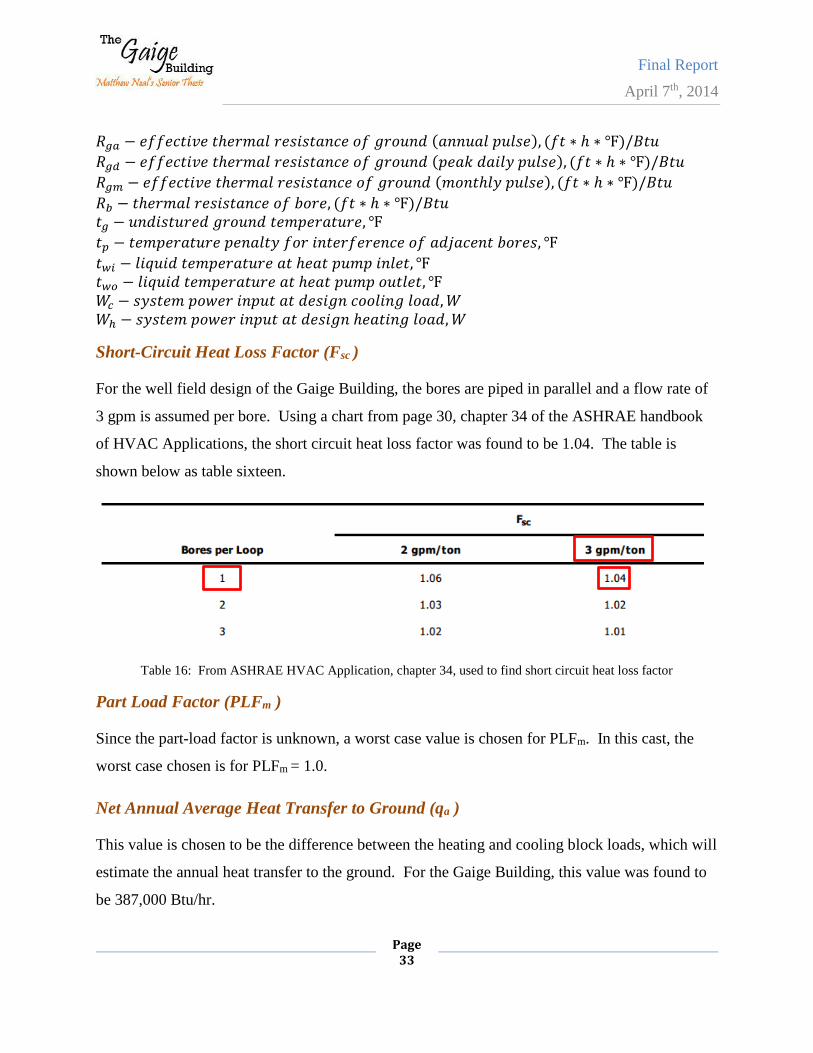
Final Report

April 7th, 2014

Page 33

𝑅𝑔𝑎 − 𝑒𝑓𝑓𝑒𝑐𝑡𝑖𝑣𝑒 𝑡ℎ𝑒𝑟𝑚𝑎𝑙 𝑟𝑒𝑠𝑖𝑠𝑡𝑎𝑛𝑐𝑒 𝑜𝑓 𝑔𝑟𝑜𝑢𝑛𝑑 (𝑎𝑛𝑛𝑢𝑎𝑙 𝑝𝑢𝑙𝑠𝑒), (𝑓𝑡 ∗ ℎ ∗ ℉)/𝐵𝑡𝑢

𝑅𝑔𝑑 − 𝑒𝑓𝑓𝑒𝑐𝑡𝑖𝑣𝑒 𝑡ℎ𝑒𝑟𝑚𝑎𝑙 𝑟𝑒𝑠𝑖𝑠𝑡𝑎𝑛𝑐𝑒 𝑜𝑓 𝑔𝑟𝑜𝑢𝑛𝑑 (𝑝𝑒𝑎𝑘 𝑑𝑎𝑖𝑙𝑦 𝑝𝑢𝑙𝑠𝑒), (𝑓𝑡 ∗ ℎ ∗ ℉)/𝐵𝑡𝑢

𝑅𝑔𝑚 − 𝑒𝑓𝑓𝑒𝑐𝑡𝑖𝑣𝑒 𝑡ℎ𝑒𝑟𝑚𝑎𝑙 𝑟𝑒𝑠𝑖𝑠𝑡𝑎𝑛𝑐𝑒 𝑜𝑓 𝑔𝑟𝑜𝑢𝑛𝑑 (𝑚𝑜𝑛𝑡ℎ𝑙𝑦 𝑝𝑢𝑙𝑠𝑒), (𝑓𝑡 ∗ ℎ ∗ ℉)/𝐵𝑡𝑢

𝑅𝑏 − 𝑡ℎ𝑒𝑟𝑚𝑎𝑙 𝑟𝑒𝑠𝑖𝑠𝑡𝑎𝑛𝑐𝑒 𝑜𝑓 𝑏𝑜𝑟𝑒, (𝑓𝑡 ∗ ℎ ∗ ℉)/𝐵𝑡𝑢

𝑡𝑔 − 𝑢𝑛𝑑𝑖𝑠𝑡𝑢𝑟𝑒𝑑 𝑔𝑟𝑜𝑢𝑛𝑑 𝑡𝑒𝑚𝑝𝑒𝑟𝑎𝑡𝑢𝑟𝑒, ℉

𝑡𝑝 − 𝑡𝑒𝑚𝑝𝑒𝑟𝑎𝑡𝑢𝑟𝑒 𝑝𝑒𝑛𝑎𝑙𝑡𝑦 𝑓𝑜𝑟 𝑖𝑛𝑡𝑒𝑟𝑓𝑒𝑟𝑒𝑛𝑐𝑒 𝑜𝑓 𝑎𝑑𝑗𝑎𝑐𝑒𝑛𝑡 𝑏𝑜𝑟𝑒𝑠, ℉

𝑡𝑤𝑖 − 𝑙𝑖𝑞𝑢𝑖𝑑 𝑡𝑒𝑚𝑝𝑒𝑟𝑎𝑡𝑢𝑟𝑒 𝑎𝑡 ℎ𝑒𝑎𝑡 𝑝𝑢𝑚𝑝 𝑖𝑛𝑙𝑒𝑡, ℉

𝑡𝑤𝑜 − 𝑙𝑖𝑞𝑢𝑖𝑑 𝑡𝑒𝑚𝑝𝑒𝑟𝑎𝑡𝑢𝑟𝑒 𝑎𝑡 ℎ𝑒𝑎𝑡 𝑝𝑢𝑚𝑝 𝑜𝑢𝑡𝑙𝑒𝑡, ℉

𝑊𝑐 − 𝑠𝑦𝑠𝑡𝑒𝑚 𝑝𝑜𝑤𝑒𝑟 𝑖𝑛𝑝𝑢𝑡 𝑎𝑡 𝑑𝑒𝑠𝑖𝑔𝑛 𝑐𝑜𝑜𝑙𝑖𝑛𝑔 𝑙𝑜𝑎𝑑, 𝑊

𝑊ℎ − 𝑠𝑦𝑠𝑡𝑒𝑚 𝑝𝑜𝑤𝑒𝑟 𝑖𝑛𝑝𝑢𝑡 𝑎𝑡 𝑑𝑒𝑠𝑖𝑔𝑛 ℎ𝑒𝑎𝑡𝑖𝑛𝑔 𝑙𝑜𝑎𝑑, 𝑊

Short-Circuit Heat Loss Factor (Fsc )

For the well field design of the Gaige Building, the bores are piped in parallel and a flow rate of

3 gpm is assumed per bore. Using a chart from page 30, chapter 34 of the ASHRAE handbook

of HVAC Applications, the short circuit heat loss factor was found to be 1.04. The table is

shown below as table sixteen.

Table 16: From ASHRAE HVAC Application, chapter 34, used to find short circuit heat loss factor

Part Load Factor (PLFm )

Since the part-load factor is unknown, a worst case value is chosen for PLFm. In this cast, the

worst case chosen is for PLFm = 1.0.

Net Annual Average Heat Transfer to Ground (qa )

This value is chosen to be the difference between the heating and cooling block loads, which will

estimate the annual heat transfer to the ground. For the Gaige Building, this value was found to

be 387,000 Btu/hr.

Final Report

April 7th, 2014

Page 34

Building Design Cooling Block Load (qlc )

This value was found using the Trace 700 model that was created and validated to the Gaige

Building’s utility cost information. Using the model, the peak, or design, cooling load for the

Gaige Building is 1,066,400 Btu/hr. This is the value to which the bore lengths should be

calculated.

Building Design Heating Block Load (qlh )

The well field also needs to be calculated using the design heating load for the Gaige Building,

for the same Trace 700 model mentioned in the previous section, this value was found to be

679,400 Btu/hr.

Effective Thermal Resistance of Ground—Annual Pulse (Rga )

This ground thermal annual pulse was calculated with a bore diameter of 6 inches, and the soil

type determined as follows. The Berks campus in the geologic region termed the great valley in

Eastern Pennsylvania. From this county geology map, the location of the building site is set on

Trenton limestone and calciferous sandstone. With these two values from table five of ASHRAE

Applications chapter 34, the thermal conductivity can be used on average as 1.7 and a diffusivity

of 1.05. The results with these values calculated the effective thermal resistance of the ground

for an annual pulse to be 0.215. These calculations are laid out below in the ground thermal

resistance calculations section.

Effective Thermal Resistance of Ground—Peak Daily Pulse (Rgd )

Using the equations from the ASHRAE chapter 34, the effective thermal resistance of the ground

for a peak daily pulse was found to be 0.129. The notes for this calculation are similar to above

under Rga, and the calculations are laid out in the ground thermal resistance calculations section.

Final Report

April 7th, 2014

Page 35

Effective Thermal Resistance of Ground—Monthly Pulse (Rgm )

For a monthly pulse, the effective thermal resistance of the ground was found to be 0.207. The

notes for this calculation are similar to above under Rga, and the calculations are laid out below

in the ground thermal resistance calculations section.

Ground Thermal Resistance Calculations

For the three effective thermal resistances of the ground listed in the previous three sections, the

following equations were used to calculate the resistances.

𝑅𝑔𝑎 =𝐺𝑓−𝐺1

𝑘𝑔 𝑅𝑔𝑚 =

𝐺1−𝐺2

𝑘𝑔 𝑅𝑔𝑑 =

𝐺2

𝑘𝑔

Where the G-factors are found using figure 15, and also using the following Fourier Numbers

𝜏1 = 3650 𝑑𝑎𝑦𝑠

𝜏2 = 3650 + 30 = 3680 𝑑𝑎𝑦𝑠

𝜏𝑓 = 3650 + 30 + 0.25 = 3680.25 𝑑𝑎𝑦𝑠

𝐹𝑜𝑓 =4 ∗ 1.05 ∗ 3680.25

0.52= 61828.2 𝐹𝑜1 =

4 ∗ 1.05 ∗ (3680.25 − 3650)

0.52= 508.2

𝐹𝑜2 =4 ∗ 1.05 ∗ (3680.25 − 3680)

0.52= 4.2

From figure 15 in chapter 34 of the ASHRAE Applications:

𝐺𝑓 = 0.938 𝑎𝑛𝑑 𝐺1 = 0.572 𝑎𝑛𝑑 𝐺2 = 0.220

So with these G values,

𝑅𝑔𝑎 =0.938−0.572

1.7= 0.215 𝑅𝑔𝑚 =

0.572−0.220

1.7= 0.207 𝑅𝑔𝑑 =

0.220

1.7= 0.129

Below, the figure 15 from chapter 34 of the ASHRAE Applications is provided, labeld figure

sixteen in this report.

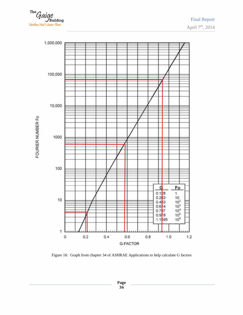
Final Report

April 7th, 2014

Page 36

Figure 16: Graph from chapter 34 of ASHRAE Applications to help calculate G factors

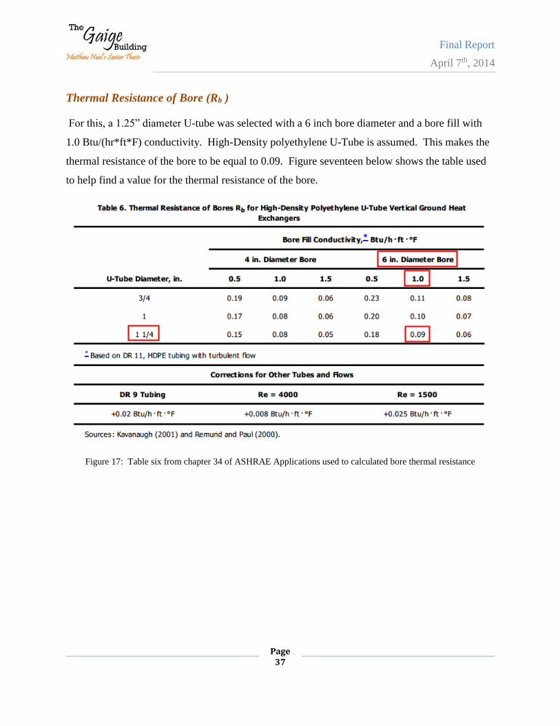
Final Report

April 7th, 2014

Page 37

Thermal Resistance of Bore (Rb )

For this, a 1.25” diameter U-tube was selected with a 6 inch bore diameter and a bore fill with

1.0 Btu/(hr*ft*F) conductivity. High-Density polyethylene U-Tube is assumed. This makes the

thermal resistance of the bore to be equal to 0.09. Figure seventeen below shows the table used

to help find a value for the thermal resistance of the bore.

Figure 17: Table six from chapter 34 of ASHRAE Applications used to calculated bore thermal resistance

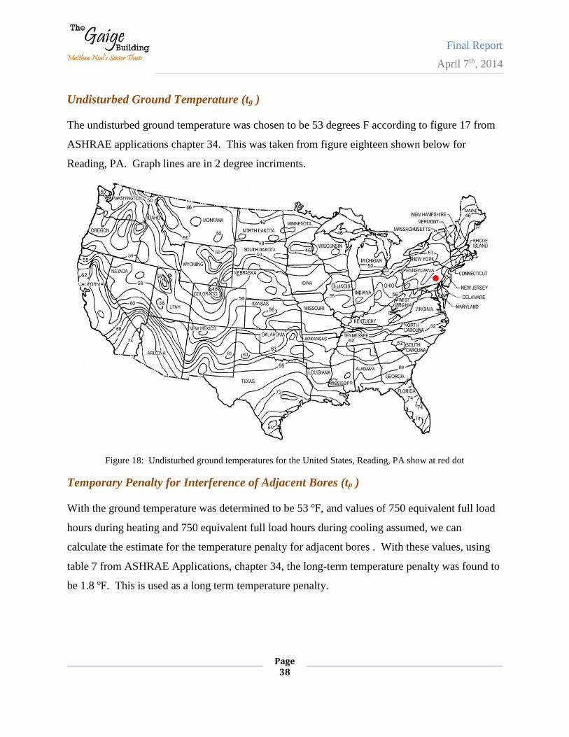
Final Report

April 7th, 2014

Page 38

Undisturbed Ground Temperature (tg )

The undisturbed ground temperature was chosen to be 53 degrees F according to figure 17 from

ASHRAE applications chapter 34. This was taken from figure eighteen shown below for

Reading, PA. Graph lines are in 2 degree incriments.

Figure 18: Undisturbed ground temperatures for the United States, Reading, PA show at red dot

Temporary Penalty for Interference of Adjacent Bores (tp )

With the ground temperature was determined to be 53 ℉, and values of 750 equivalent full load

hours during heating and 750 equivalent full load hours during cooling assumed, we can

calculate the estimate for the temperature penalty for adjacent bores . With these values, using

table 7 from ASHRAE Applications, chapter 34, the long-term temperature penalty was found to

be 1.8 ℉. This is used as a long term temperature penalty.

Final Report

April 7th, 2014

Page 39

Liquid Temperature at Heat Pump Inlet (twi )

The water temperature at the inlet to the geothermal bores is chosen relative to the ground

temperature, of 53 ℉. For cooling, the temperature is typically chosen to be 20 ℉ to 30 ℉

higher than undisturbed ground temperature for cooling and 10 ℉ to 20 ℉ lower for heating. For

this test, 78 ℉ is used for cooling and 38 ℉ is used for heating.

Liquid Temperature at Heat Pump Outlet (two )

These values were chosen to be roughly five to seven degrees different from the entering

temperature to the heat pumps. The value increases for cooling mode, and decreases for heating

mode. To ensure that freezing would not be an issue, this system design was chose to use a

heating outlet temperature of 33 degrees and a cooling outlet temperature of 85 degrees.

System Power Input at Design Cooling Load (Wc )

For the geothermal well field, once the overall well field was designed, the pump head for the

system and flow rate was used to help select a pump for the geothermal well field. Once the

initial pump was found, which will be provided in the equipment selection section 3.1.6 below,

the input power to the system was found to be 3728.5 W, calculated from the pumps horse

power.

System Power Input at Design Heating Load (Wh )

The pump chosen for the system for cooling will be the same pump chosen for heating. Thus,

the input power to the system during heating will also be 3728.5 W.

Final Geothermal Length Calculations

Below, table x summarizes the previously listed values and performing the calculations for Lc

and Lh from the equations at the beginning of this section.

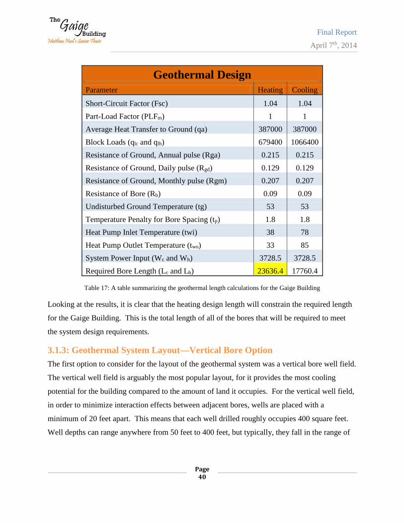
Final Report

April 7th, 2014

Page 40

Geothermal Design

Parameter Heating Cooling

Short-Circuit Factor (Fsc) 1.04 1.04

Part-Load Factor (PLFm) 1 1

Average Heat Transfer to Ground (qa) 387000 387000

Block Loads (qlc and qlh) 679400 1066400

Resistance of Ground, Annual pulse (Rga) 0.215 0.215

Resistance of Ground, Daily pulse (Rgd) 0.129 0.129

Resistance of Ground, Monthly pulse (Rgm) 0.207 0.207

Resistance of Bore (Rb) 0.09 0.09

Undisturbed Ground Temperature (tg) 53 53

Temperature Penalty for Bore Spacing (tp) 1.8 1.8

Heat Pump Inlet Temperature (twi) 38 78

Heat Pump Outlet Temperature (two) 33 85

System Power Input (Wc and Wh) 3728.5 3728.5

Required Bore Length (Lc and Lh) 23636.4 17760.4

Table 17: A table summarizing the geothermal length calculations for the Gaige Building

Looking at the results, it is clear that the heating design length will constrain the required length

for the Gaige Building. This is the total length of all of the bores that will be required to meet

the system design requirements.

3.1.3: Geothermal System Layout—Vertical Bore Option

The first option to consider for the layout of the geothermal system was a vertical bore well field.

The vertical well field is arguably the most popular layout, for it provides the most cooling

potential for the building compared to the amount of land it occupies. For the vertical well field,

in order to minimize interaction effects between adjacent bores, wells are placed with a

minimum of 20 feet apart. This means that each well drilled roughly occupies 400 square feet.

Well depths can range anywhere from 50 feet to 400 feet, but typically, they fall in the range of

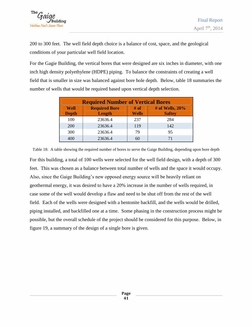
Final Report

April 7th, 2014

Page 41

200 to 300 feet. The well field depth choice is a balance of cost, space, and the geological

conditions of your particular well field location.

For the Gagie Building, the vertical bores that were designed are six inches in diameter, with one

inch high density polyethylene (HDPE) piping. To balance the constraints of creating a well

field that is smaller in size was balanced against bore hole depth. Below, table 18 summaries the

number of wells that would be required based upon vertical depth selection.

Required Number of Vertical Bores Well

Depth

Required Bore

Length

# of

Wells

# of Wells, 20%

Saftey

100 23636.4 237 284

200 23636.4 119 142

300 23636.4 79 95

400 23636.4 60 71

Table 18: A table showing the required number of bores to serve the Gaige Building, depending upon bore depth

For this building, a total of 100 wells were selected for the well field design, with a depth of 300

feet. This was chosen as a balance between total number of wells and the space it would occupy.

Also, since the Gaige Building’s new opposed energy source will be heavily reliant on

geothermal energy, it was desired to have a 20% increase in the number of wells required, in

case some of the well would develop a flaw and need to be shut off from the rest of the well

field. Each of the wells were designed with a bentonite backfill, and the wells would be drilled,

piping installed, and backfilled one at a time. Some phasing in the construction process might be

possible, but the overall schedule of the project should be considered for this purpose. Below, in

figure 19, a summary of the design of a single bore is given.

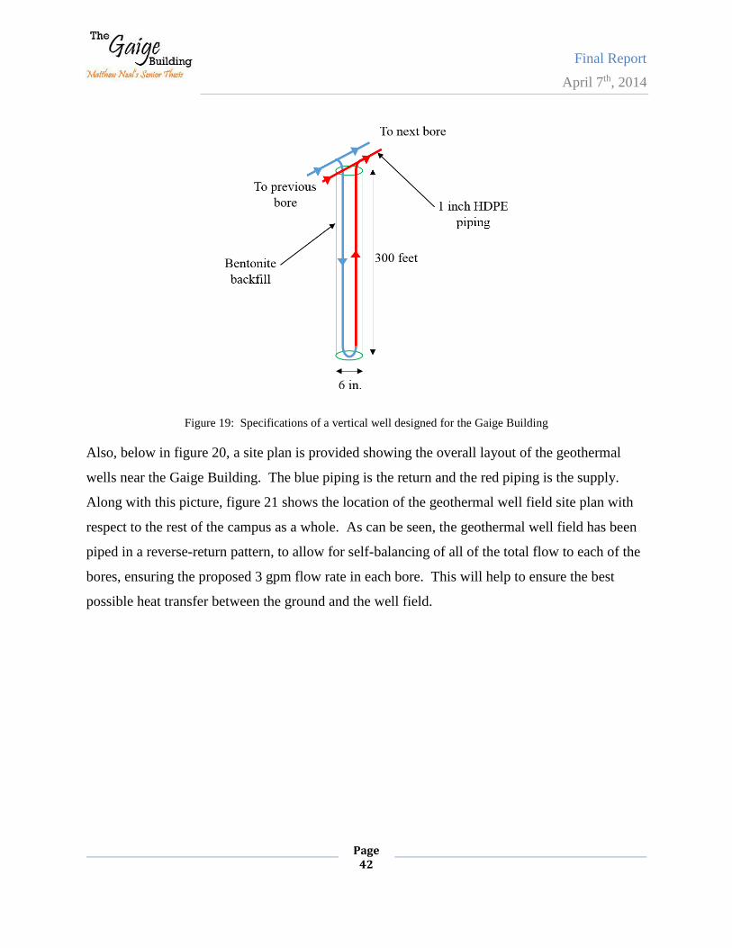
Final Report

April 7th, 2014

Page 42

Figure 19: Specifications of a vertical well designed for the Gaige Building

Also, below in figure 20, a site plan is provided showing the overall layout of the geothermal

wells near the Gaige Building. The blue piping is the return and the red piping is the supply.

Along with this picture, figure 21 shows the location of the geothermal well field site plan with

respect to the rest of the campus as a whole. As can be seen, the geothermal well field has been

piped in a reverse-return pattern, to allow for self-balancing of all of the total flow to each of the

bores, ensuring the proposed 3 gpm flow rate in each bore. This will help to ensure the best

possible heat transfer between the ground and the well field.

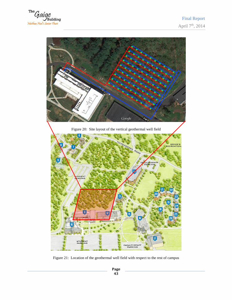
Final Report

April 7th, 2014

Page 43

Figure 20: Site layout of the vertical geothermal well field

Figure 21: Location of the geothermal well field with respect to the rest of campus

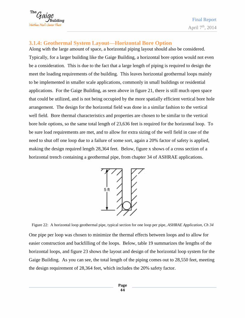
Final Report

April 7th, 2014

Page 44

3.1.4: Geothermal System Layout—Horizontal Bore Option Along with the large amount of space, a horizontal piping layout should also be considered.

Typically, for a larger building like the Gaige Building, a horizontal bore option would not even

be a consideration. This is due to the fact that a large length of piping is required to design the

meet the loading requirements of the building. This leaves horizontal geothermal loops mainly

to be implemented in smaller scale applications, commonly in small buildings or residential

applications. For the Gaige Building, as seen above in figure 21, there is still much open space

that could be utilized, and is not being occupied by the more spatially efficient vertical bore hole

arrangement. The design for the horizontal field was done in a similar fashion to the vertical

well field. Bore thermal characteristics and properties are chosen to be similar to the vertical

bore hole options, so the same total length of 23,636 feet is required for the horizontal loop. To

be sure load requirements are met, and to allow for extra sizing of the well field in case of the

need to shut off one loop due to a failure of some sort, again a 20% factor of safety is applied,

making the design required length 28,364 feet. Below, figure x shows of a cross section of a

horizontal trench containing a geothermal pipe, from chapter 34 of ASHRAE applications.

Figure 22: A horizontal loop geothermal pipe, typical section for one loop per pipe, ASHRAE Application, Ch 34

One pipe per loop was chosen to minimize the thermal effects between loops and to allow for

easier construction and backfilling of the loops. Below, table 19 summarizes the lengths of the

horizontal loops, and figure 23 shows the layout and design of the horizontal loop system for the

Gaige Building. As you can see, the total length of the piping comes out to 28,550 feet, meeting

the design requirement of 28,364 feet, which includes the 20% safety factor.

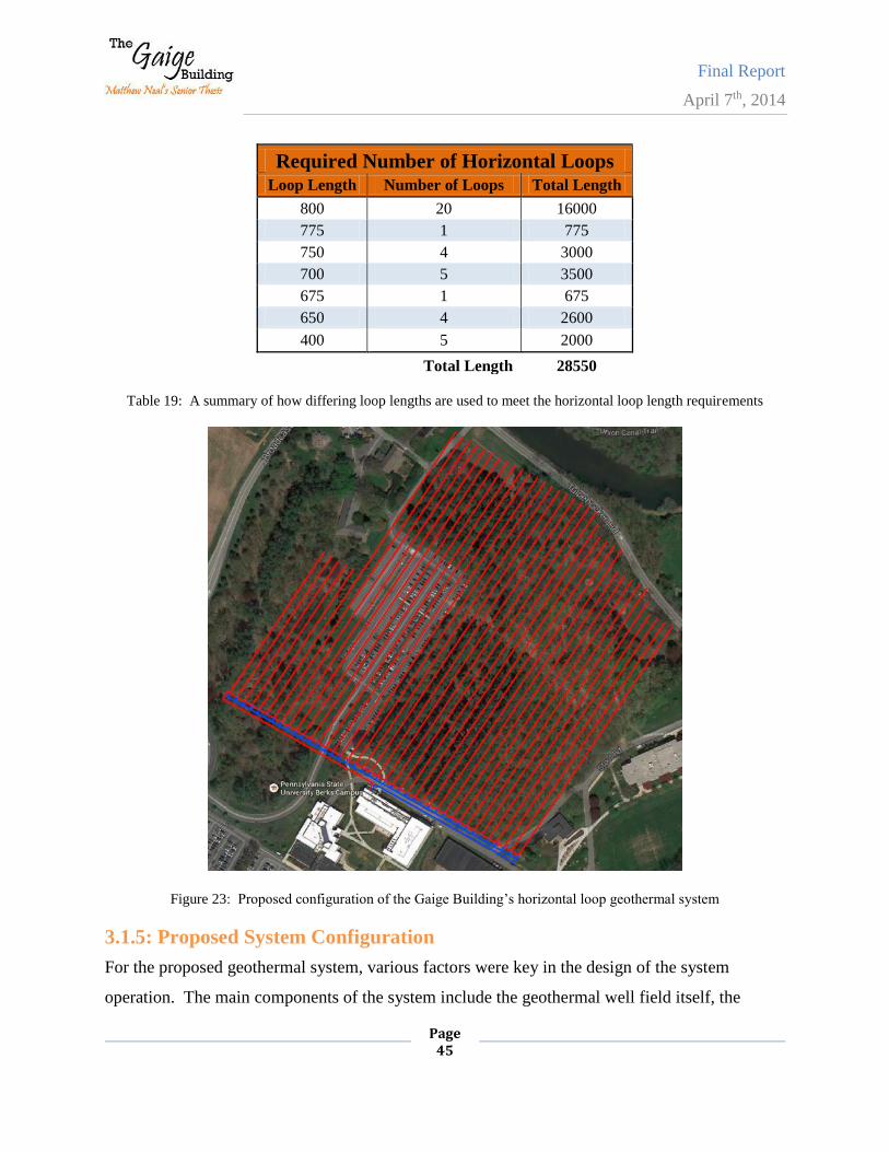
Final Report

April 7th, 2014

Page 45

Required Number of Horizontal Loops Loop Length Number of Loops Total Length

800 20 16000

775 1 775

750 4 3000

700 5 3500

675 1 675

650 4 2600

400 5 2000

Total Length 28550

Table 19: A summary of how differing loop lengths are used to meet the horizontal loop length requirements

Figure 23: Proposed configuration of the Gaige Building’s horizontal loop geothermal system

3.1.5: Proposed System Configuration

For the proposed geothermal system, various factors were key in the design of the system

operation. The main components of the system include the geothermal well field itself, the

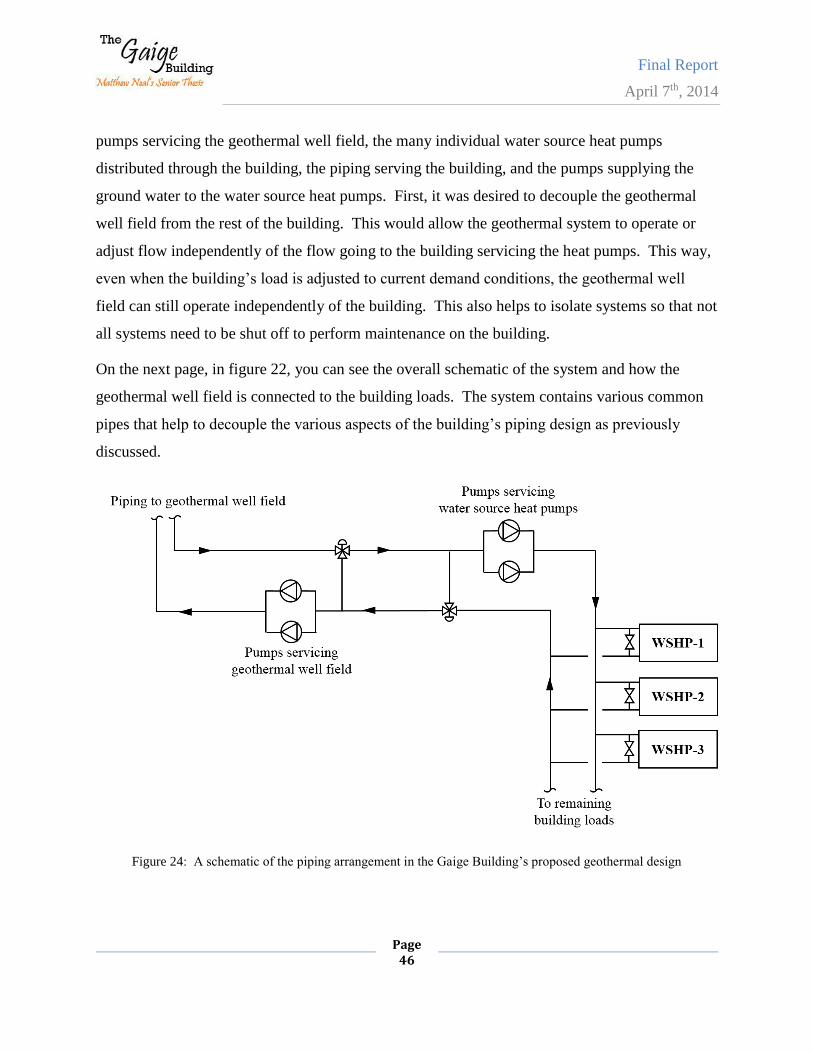
Final Report

April 7th, 2014

Page 46

pumps servicing the geothermal well field, the many individual water source heat pumps

distributed through the building, the piping serving the building, and the pumps supplying the

ground water to the water source heat pumps. First, it was desired to decouple the geothermal

well field from the rest of the building. This would allow the geothermal system to operate or

adjust flow independently of the flow going to the building servicing the heat pumps. This way,

even when the building’s load is adjusted to current demand conditions, the geothermal well

field can still operate independently of the building. This also helps to isolate systems so that not

all systems need to be shut off to perform maintenance on the building.

On the next page, in figure 22, you can see the overall schematic of the system and how the

geothermal well field is connected to the building loads. The system contains various common

pipes that help to decouple the various aspects of the building’s piping design as previously

discussed.

Figure 24: A schematic of the piping arrangement in the Gaige Building’s proposed geothermal design

Final Report

April 7th, 2014

Page 47

Along with servicing heat pumps placed in each of the building spaces, the geothermal loop will

also serve a larger capacity water source heat pump that will service the heating / cooling coil for

the dedicated outdoor air unit. Also, with hot water demand for the building, a boiler will be

provided to supply the hot water to the building. The boiler will also be sized to provide

supplemental hot water to the heating coils, in case the geothermal system cannot fully meet the

heating load. This design of having a backup boiler in the system was included in the energy

model for the space, so it will also potentially supplement the water system as well during

heating season.

3.1.6: Building Piping Layout

In order to implement a new ground loop into the Gaige Building, not only must the pumps be

sized and placed in the mechanical room, but a piping distribution plan must be laid out within

the building, and space considerations must be made. The ground loop will enter into the

building on the first floor, coming into the mechanical room in the upper left corner of the

building. There is currently a large amount of space in that mechanical room, so space concerns

will not be an issue when placing the additional pumps required in the Gaige Building’s design.

It is proposed that the ground water loop be piped throughout the building through a central pipe

run that passes through the main circulation corridor of the building. This piping will be exposed

in the main corridor, for it has an open atrium style plan, and then it will run above the drop

acoustical ceiling tile when it circulates through the office spaces. Below, main piing runs are

shown for the first, second, and third floor, in figures 23, 24, and 25 respectively.

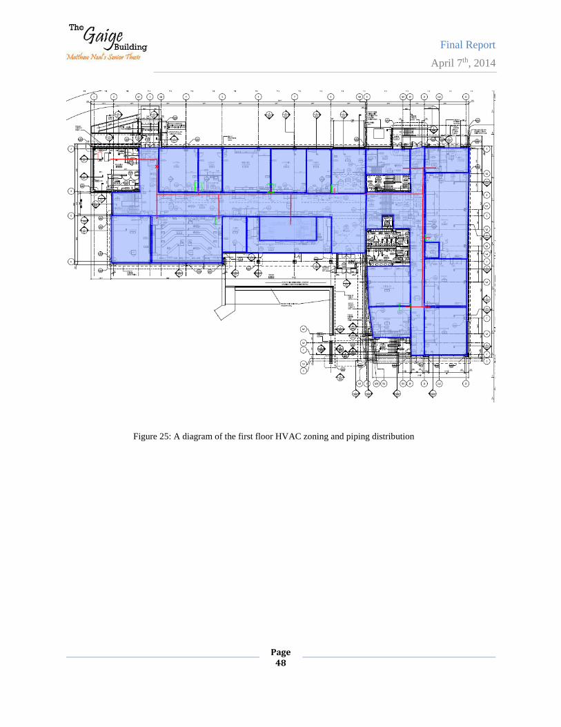
Final Report

April 7th, 2014

Page 48

Figure 25: A diagram of the first floor HVAC zoning and piping distribution

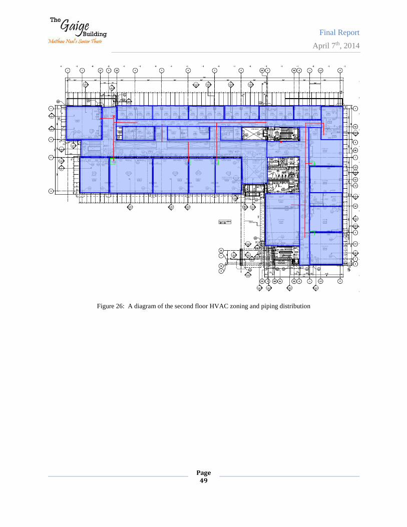
Final Report

April 7th, 2014

Page 49

Figure 26: A diagram of the second floor HVAC zoning and piping distribution

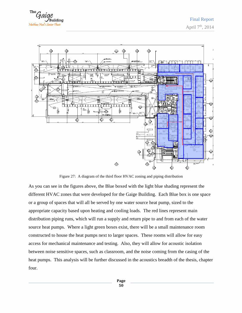
Final Report

April 7th, 2014

Page 50

Figure 27: A diagram of the third floor HVAC zoning and piping distribution

As you can see in the figures above, the Blue boxed with the light blue shading represent the

different HVAC zones that were developed for the Gaige Building. Each Blue box is one space

or a group of spaces that will all be served by one water source heat pump, sized to the

appropriate capacity based upon heating and cooling loads. The red lines represent main

distribution piping runs, which will run a supply and return pipe to and from each of the water

source heat pumps. Where a light green boxes exist, there will be a small maintenance room

constructed to house the heat pumps next to larger spaces. These rooms will allow for easy

access for mechanical maintenance and testing. Also, they will allow for acoustic isolation

between noise sensitive spaces, such as classroom, and the noise coming from the casing of the

heat pumps. This analysis will be further discussed in the acoustics breadth of the thesis, chapter

four.

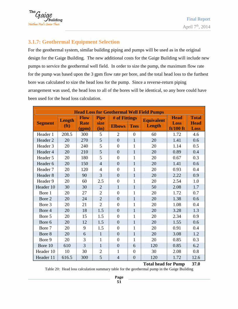
Final Report

April 7th, 2014

Page 51

3.1.7: Geothermal Equipment Selection

For the geothermal system, similar building piping and pumps will be used as in the original

design for the Gaige Building. The new additional costs for the Gaige Building will include new

pumps to service the geothermal well field. In order to size the pump, the maximum flow rate

for the pump was based upon the 3 gpm flow rate per bore, and the total head loss to the furthest

bore was calculated to size the head loss for the pump. Since a reverse-return piping

arrangement was used, the head loss to all of the bores will be identical, so any bore could have

been used for the head loss calculation.

Head Loss for Geothermal Well Field Pumps

Segment Length

(ft)

Flow

Rate

(gpm)

Pipe

size

(in)

# of Fittings Equivalent

Length

Head

Loss

ft/100 ft

Total

Head

Loss Elbows Tees

Header 1 208.5 300 5 2 0 60 1.72 4.6

Header 2 20 270 5 0 1 20 1.41 0.6

Header 3 20 240 5 0 1 20 1.14 0.5

Header 4 20 210 5 0 1 20 0.89 0.4

Header 5 20 180 5 0 1 20 0.67 0.3

Header 6 20 150 4 0 1 20 1.41 0.6

Header 7 20 120 4 0 1 20 0.93 0.4

Header 8 20 90 3 0 1 20 2.22 0.9

Header 9 20 60 2.5 0 1 20 2.54 1.0

Header 10 30 30 2 1 1 50 2.08 1.7

Bore 1 20 27 2 0 1 20 1.72 0.7

Bore 2 20 24 2 0 1 20 1.38 0.6

Bore 3 20 21 2 0 1 20 1.08 0.4

Bore 4 20 18 1.5 0 1 20 3.28 1.3

Bore 5 20 15 1.5 0 1 20 2.34 0.9

Bore 6 20 12 1.5 0 1 20 1.55 0.6

Bore 7 20 9 1.5 0 1 20 0.91 0.4

Bore 8 20 6 1 0 1 20 3.08 1.2

Bore 9 20 3 1 0 1 20 0.85 0.3

Bore 10 610 3 1 0 6 120 0.85 6.2

Header 10 10 30 2 1 0 30 2.08 0.8

Header 11 616.5 300 5 4 0 120 1.72 12.6

Total head for Pump 37.0 Table 20: Head loss calculation summary table for the geothermal pump in the Gaige Building

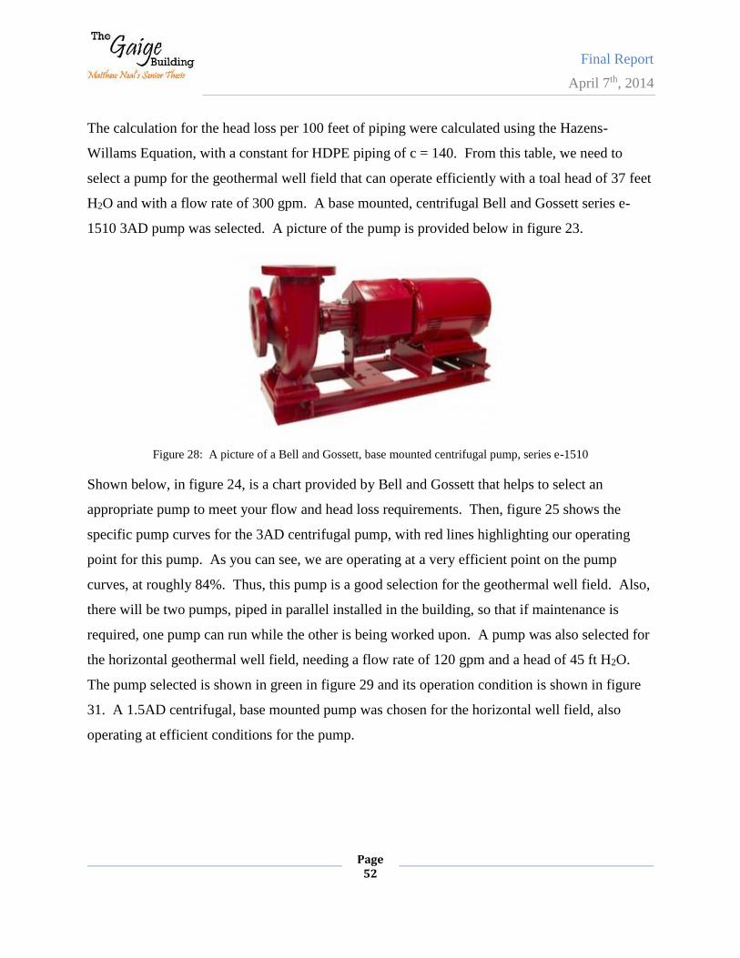
Final Report

April 7th, 2014

Page 52

The calculation for the head loss per 100 feet of piping were calculated using the Hazens-

Willams Equation, with a constant for HDPE piping of c = 140. From this table, we need to

select a pump for the geothermal well field that can operate efficiently with a toal head of 37 feet

H2O and with a flow rate of 300 gpm. A base mounted, centrifugal Bell and Gossett series e-

1510 3AD pump was selected. A picture of the pump is provided below in figure 23.

Figure 28: A picture of a Bell and Gossett, base mounted centrifugal pump, series e-1510

Shown below, in figure 24, is a chart provided by Bell and Gossett that helps to select an

appropriate pump to meet your flow and head loss requirements. Then, figure 25 shows the

specific pump curves for the 3AD centrifugal pump, with red lines highlighting our operating

point for this pump. As you can see, we are operating at a very efficient point on the pump

curves, at roughly 84%. Thus, this pump is a good selection for the geothermal well field. Also,

there will be two pumps, piped in parallel installed in the building, so that if maintenance is

required, one pump can run while the other is being worked upon. A pump was also selected for

the horizontal geothermal well field, needing a flow rate of 120 gpm and a head of 45 ft H2O.

The pump selected is shown in green in figure 29 and its operation condition is shown in figure

31. A 1.5AD centrifugal, base mounted pump was chosen for the horizontal well field, also

operating at efficient conditions for the pump.

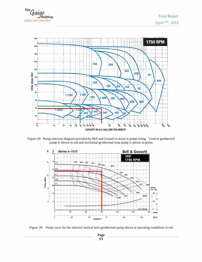
Final Report

April 7th, 2014

Page 53

Figure 29: Pump selection diagram provided by Bell and Gossett to assist in pump sizing. Vertical geothermal

pump is shown in red and horizontal geothermal loop pump is shown in green

Figure 30: Pump curve for the selected vertical bore geothermal pump shown at operating conditions in red

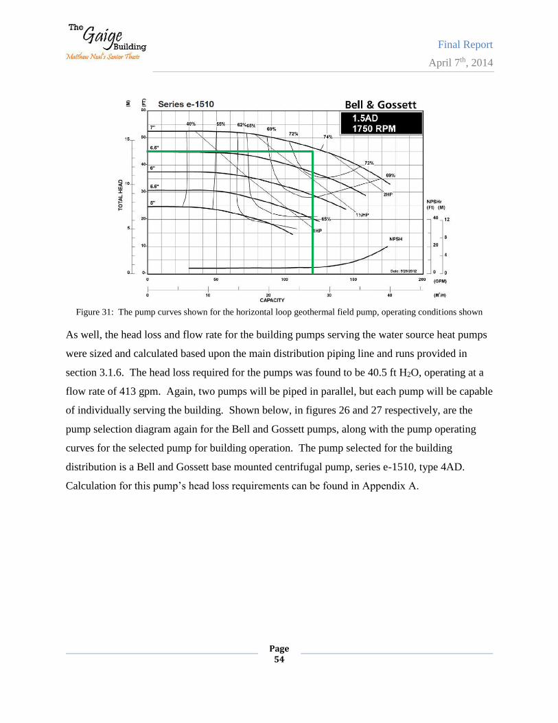
Final Report

April 7th, 2014

Page 54

Figure 31: The pump curves shown for the horizontal loop geothermal field pump, operating conditions shown

As well, the head loss and flow rate for the building pumps serving the water source heat pumps

were sized and calculated based upon the main distribution piping line and runs provided in

section 3.1.6. The head loss required for the pumps was found to be 40.5 ft H2O, operating at a

flow rate of 413 gpm. Again, two pumps will be piped in parallel, but each pump will be capable

of individually serving the building. Shown below, in figures 26 and 27 respectively, are the

pump selection diagram again for the Bell and Gossett pumps, along with the pump operating

curves for the selected pump for building operation. The pump selected for the building

distribution is a Bell and Gossett base mounted centrifugal pump, series e-1510, type 4AD.

Calculation for this pump’s head loss requirements can be found in Appendix A.

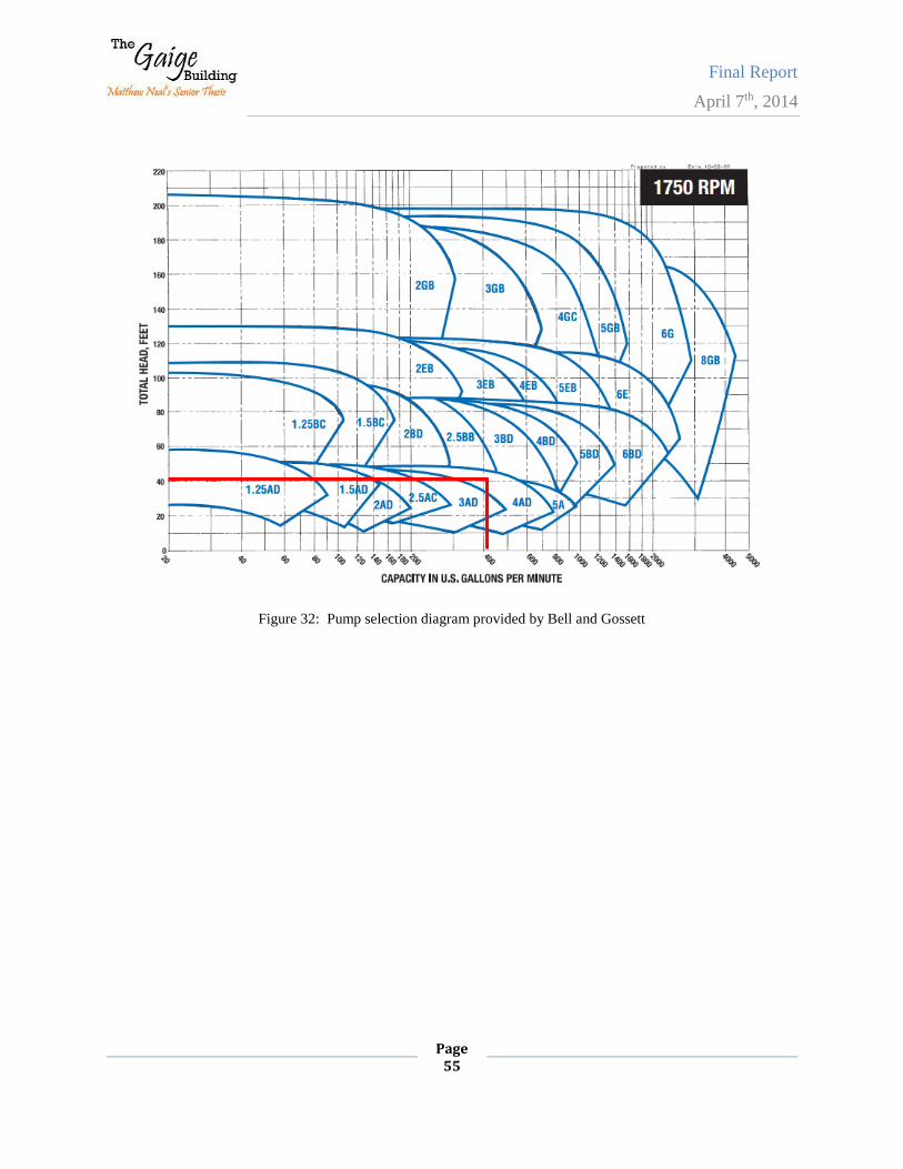
Final Report

April 7th, 2014

Page 55

Figure 32: Pump selection diagram provided by Bell and Gossett

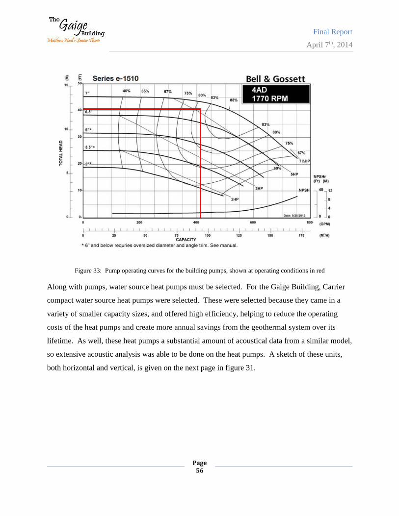
Final Report

April 7th, 2014

Page 56

Figure 33: Pump operating curves for the building pumps, shown at operating conditions in red

Along with pumps, water source heat pumps must be selected. For the Gaige Building, Carrier

compact water source heat pumps were selected. These were selected because they came in a

variety of smaller capacity sizes, and offered high efficiency, helping to reduce the operating

costs of the heat pumps and create more annual savings from the geothermal system over its

lifetime. As well, these heat pumps a substantial amount of acoustical data from a similar model,

so extensive acoustic analysis was able to be done on the heat pumps. A sketch of these units,

both horizontal and vertical, is given on the next page in figure 31.

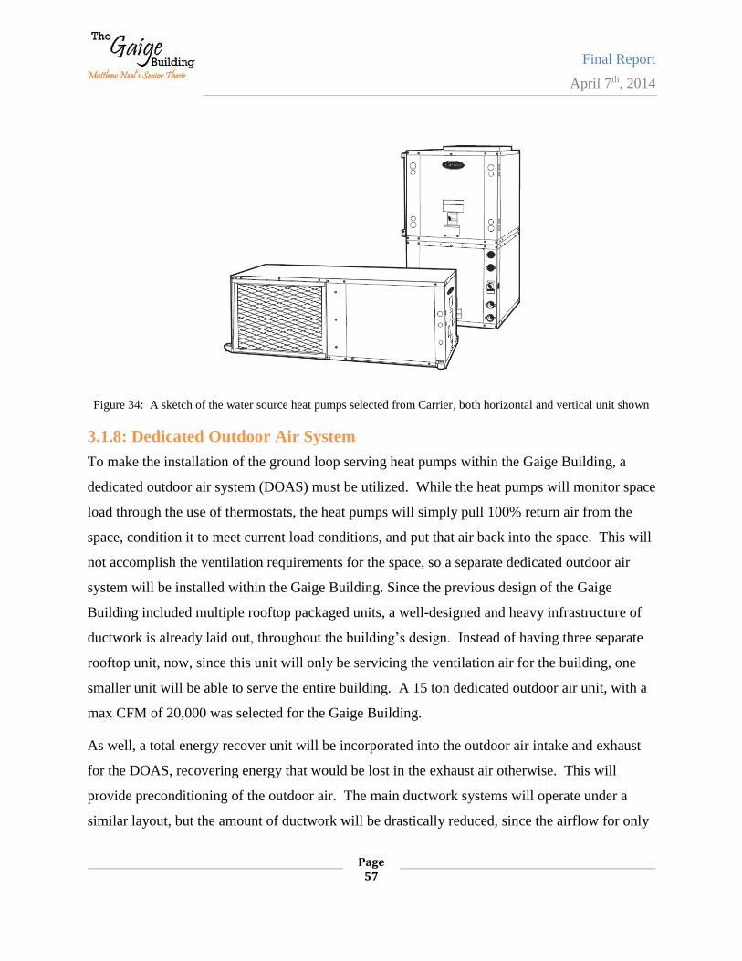
Final Report

April 7th, 2014

Page 57

Figure 34: A sketch of the water source heat pumps selected from Carrier, both horizontal and vertical unit shown

3.1.8: Dedicated Outdoor Air System

To make the installation of the ground loop serving heat pumps within the Gaige Building, a

dedicated outdoor air system (DOAS) must be utilized. While the heat pumps will monitor space

load through the use of thermostats, the heat pumps will simply pull 100% return air from the

space, condition it to meet current load conditions, and put that air back into the space. This will

not accomplish the ventilation requirements for the space, so a separate dedicated outdoor air

system will be installed within the Gaige Building. Since the previous design of the Gaige

Building included multiple rooftop packaged units, a well-designed and heavy infrastructure of

ductwork is already laid out, throughout the building’s design. Instead of having three separate

rooftop unit, now, since this unit will only be servicing the ventilation air for the building, one

smaller unit will be able to serve the entire building. A 15 ton dedicated outdoor air unit, with a

max CFM of 20,000 was selected for the Gaige Building.

As well, a total energy recover unit will be incorporated into the outdoor air intake and exhaust

for the DOAS, recovering energy that would be lost in the exhaust air otherwise. This will

provide preconditioning of the outdoor air. The main ductwork systems will operate under a

similar layout, but the amount of ductwork will be drastically reduced, since the airflow for only

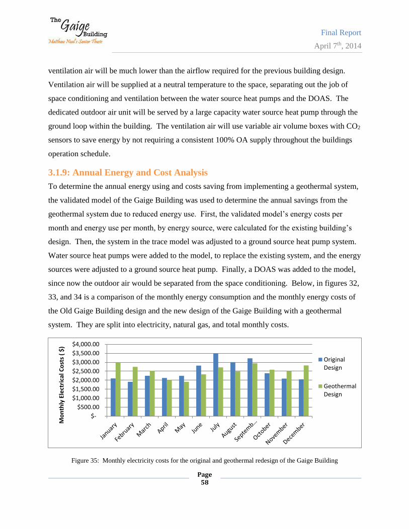
Final Report

April 7th, 2014

Page 58

ventilation air will be much lower than the airflow required for the previous building design.

Ventilation air will be supplied at a neutral temperature to the space, separating out the job of

space conditioning and ventilation between the water source heat pumps and the DOAS. The

dedicated outdoor air unit will be served by a large capacity water source heat pump through the

ground loop within the building. The ventilation air will use variable air volume boxes with CO2

sensors to save energy by not requiring a consistent 100% OA supply throughout the buildings

operation schedule.

3.1.9: Annual Energy and Cost Analysis

To determine the annual energy using and costs saving from implementing a geothermal system,

the validated model of the Gaige Building was used to determine the annual savings from the

geothermal system due to reduced energy use. First, the validated model’s energy costs per

month and energy use per month, by energy source, were calculated for the existing building’s

design. Then, the system in the trace model was adjusted to a ground source heat pump system.

Water source heat pumps were added to the model, to replace the existing system, and the energy

sources were adjusted to a ground source heat pump. Finally, a DOAS was added to the model,

since now the outdoor air would be separated from the space conditioning. Below, in figures 32,

33, and 34 is a comparison of the monthly energy consumption and the monthly energy costs of

the Old Gaige Building design and the new design of the Gaige Building with a geothermal

system. They are split into electricity, natural gas, and total monthly costs.

Figure 35: Monthly electricity costs for the original and geothermal redesign of the Gaige Building

$-

$500.00

$1,000.00

$1,500.00

$2,000.00

$2,500.00

$3,000.00

$3,500.00

$4,000.00

Mo

nth

ly E

lect

rica

l Co

sts

( $

)

OriginalDesign

GeothermalDesign

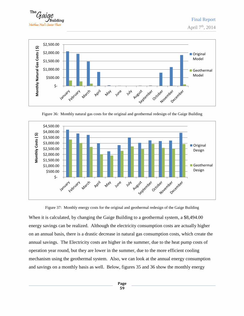
Final Report

April 7th, 2014

Page 59

Figure 36: Monthly natural gas costs for the original and geothermal redesign of the Gaige Building

Figure 37: Monthly energy costs for the original and geothermal redesign of the Gaige Building

When it is calculated, by changing the Gaige Building to a geothermal system, a $8,494.00

energy savings can be realized. Although the electricity consumption costs are actually higher

on an annual basis, there is a drastic decrease in natural gas consumption costs, which create the

annual savings. The Electricity costs are higher in the summer, due to the heat pump costs of

operation year round, but they are lower in the summer, due to the more efficient cooling

mechanism using the geothermal system. Also, we can look at the annual energy consumption

and savings on a monthly basis as well. Below, figures 35 and 36 show the monthly energy

$-

$500.00

$1,000.00

$1,500.00

$2,000.00

$2,500.00

Mo

nth

ly N

atu

ral G

as C

ost

s (

$)

OriginalModel

GeothermalModel

$-

$500.00

$1,000.00

$1,500.00

$2,000.00

$2,500.00

$3,000.00

$3,500.00

$4,000.00

$4,500.00

Mo

nth

ly C

ost

s (

$)

OriginalDesign

GeothermalDesign

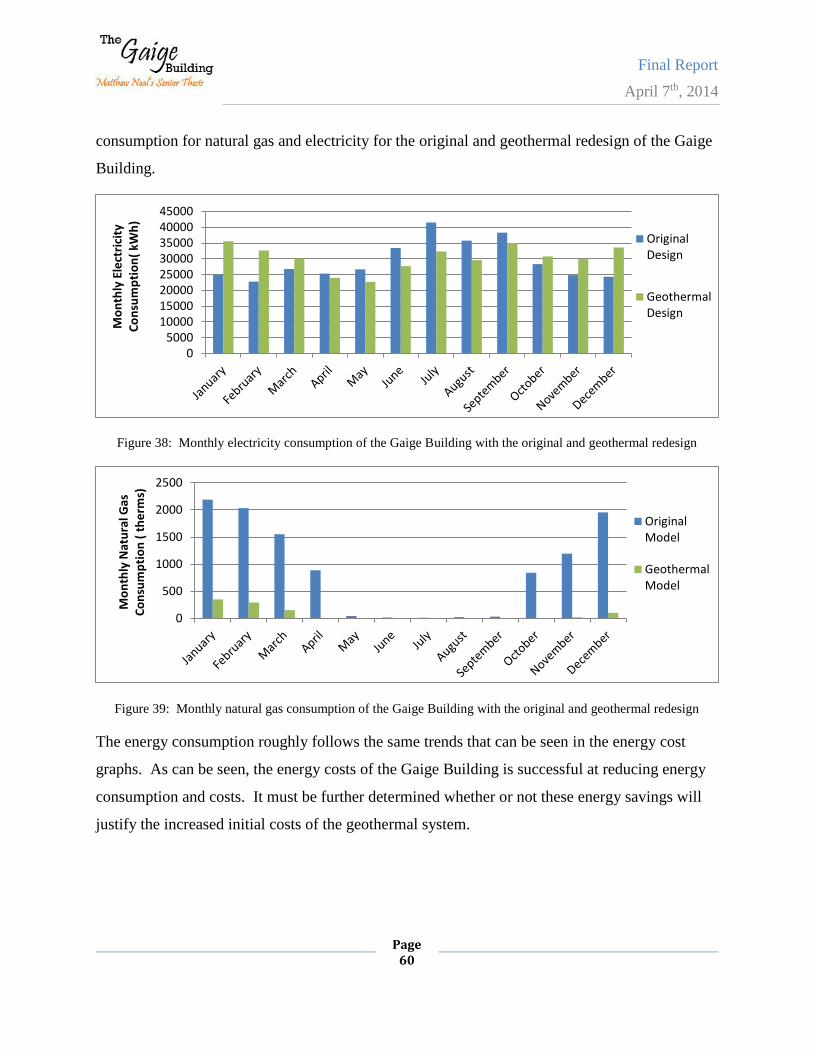
Final Report

April 7th, 2014

Page 60

consumption for natural gas and electricity for the original and geothermal redesign of the Gaige

Building.

Figure 38: Monthly electricity consumption of the Gaige Building with the original and geothermal redesign

Figure 39: Monthly natural gas consumption of the Gaige Building with the original and geothermal redesign

The energy consumption roughly follows the same trends that can be seen in the energy cost

graphs. As can be seen, the energy costs of the Gaige Building is successful at reducing energy

consumption and costs. It must be further determined whether or not these energy savings will

justify the increased initial costs of the geothermal system.

05000

1000015000200002500030000350004000045000

Mo

nth

ly E

lect

rici

ty

Co

nsu

mp

tio

n(

kWh

)

OriginalDesign

GeothermalDesign

0

500

1000

1500

2000

2500

Mo

nth

ly N

atu

ral G

as

Co

nsu

mp

tio

n (

th

erm

s)

OriginalModel

GeothermalModel

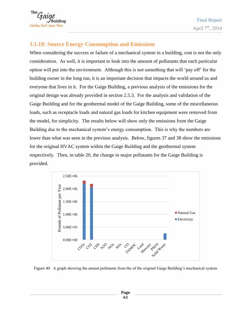
Final Report

April 7th, 2014

Page 61

3.1.10: Source Energy Consumption and Emissions

When considering the success or failure of a mechanical system in a building, cost is not the only

consideration. As well, it is important to look into the amount of pollutants that each particular

option will put into the environment. Although this is not something that will ‘pay off’ for the

building owner in the long run, it is an important decision that impacts the world around us and

everyone that lives in it. For the Gaige Building, a previous analysis of the emissions for the

original design was already provided in section 2.5.3. For the analysis and validation of the

Gaige Building and for the geothermal model of the Gaige Building, some of the miscellaneous

loads, such as receptacle loads and natural gas loads for kitchen equipment were removed from

the model, for simplicity. The results below will show only the emissions from the Gaige

Building due to the mechanical system’s energy consumption. This is why the numbers are

lower than what was seen in the previous analysis. Below, figures 37 and 38 show the emissions

for the original HVAC system within the Gaige Building and the geothermal system

respectively. Then, in table 20, the change in major pollutants for the Gaige Building is

provided.

Figure 40: A graph showing the annual pollutants from the of the original Gaige Building’s mechanical system

0.00E+00

5.00E+05

1.00E+06

1.50E+06

2.00E+06

2.50E+06

Po

und

s o

f P

oll

uta

nt

per

Yea

r

Natural Gas

Electricity

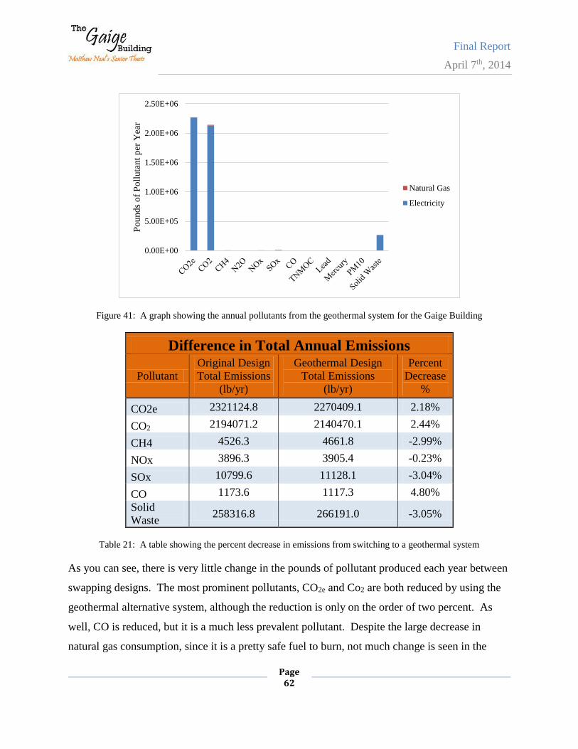
Final Report

April 7th, 2014

Page 62

Figure 41: A graph showing the annual pollutants from the geothermal system for the Gaige Building

Difference in Total Annual Emissions

Pollutant

Original Design

Total Emissions

(lb/yr)

Geothermal Design

Total Emissions

(lb/yr)

Percent

Decrease

%

CO2e 2321124.8 2270409.1 2.18%

CO2 2194071.2 2140470.1 2.44%

CH4 4526.3 4661.8 -2.99%

NOx 3896.3 3905.4 -0.23%

SOx 10799.6 11128.1 -3.04%

CO 1173.6 1117.3 4.80%

Solid

Waste 258316.8 266191.0 -3.05%

Table 21: A table showing the percent decrease in emissions from switching to a geothermal system

As you can see, there is very little change in the pounds of pollutant produced each year between

swapping designs. The most prominent pollutants, CO2e and Co2 are both reduced by using the

geothermal alternative system, although the reduction is only on the order of two percent. As

well, CO is reduced, but it is a much less prevalent pollutant. Despite the large decrease in

natural gas consumption, since it is a pretty safe fuel to burn, not much change is seen in the

0.00E+00

5.00E+05

1.00E+06

1.50E+06

2.00E+06

2.50E+06

Po

und

s o

f P

oll

uta

nt

per

Yea

r

Natural Gas

Electricity

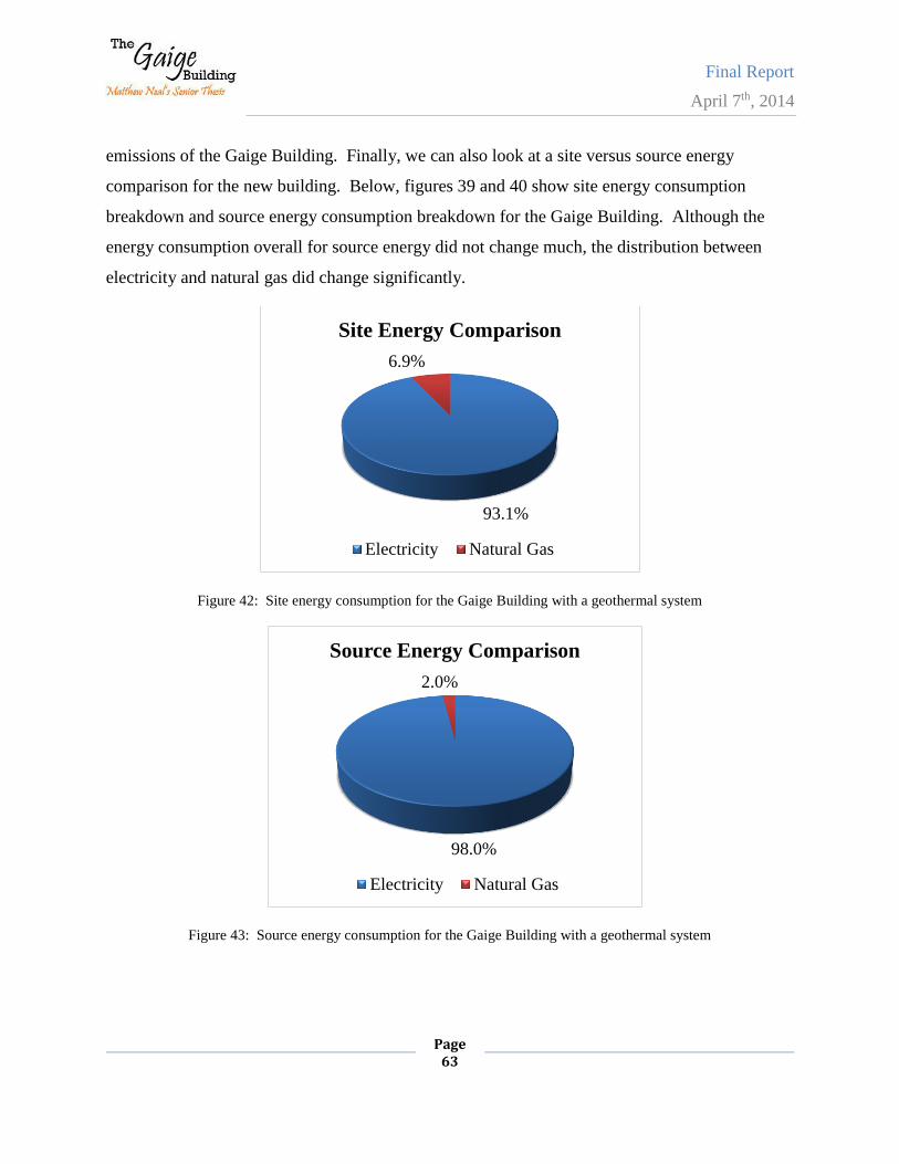
Final Report

April 7th, 2014

Page 63

emissions of the Gaige Building. Finally, we can also look at a site versus source energy

comparison for the new building. Below, figures 39 and 40 show site energy consumption

breakdown and source energy consumption breakdown for the Gaige Building. Although the

energy consumption overall for source energy did not change much, the distribution between

electricity and natural gas did change significantly.

Figure 42: Site energy consumption for the Gaige Building with a geothermal system

Figure 43: Source energy consumption for the Gaige Building with a geothermal system

93.1%

6.9%

Site Energy Comparison


98.0%

2.0%

Source Energy Comparison


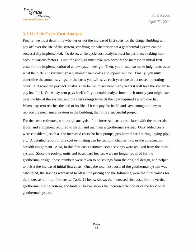
Final Report

April 7th, 2014

Page 64

3.1.11: Life Cycle Cost Analysis

Finally, we must determine whether or not the increased first costs for the Gaige Building will

pay off over the life of the system, verifying the whether or not a geothermal system can be

successfully implemented. To do so, a life cycle cost analysis must be performed taking into

account various factors. First, the analysis must take into account the increase in initial first

costs for the implementation of a new system design. Then, you must also make judgments as to

what the different systems’ yearly maintenance costs and repairs will be. Finally, you must

determine the annual savings, or the costs you will save each year due to decreased operating

costs. A discounted payback analysis can be run to see how many years it will take the system to

pay itself off. Once a system pays itself off, you could analyze how much money you might save

over the life of the system, and put that savings towards the next required system overhaul.

When a system reaches the end of its life, if it can pay for itself, and save enough money to

replace the mechanical system in the building, then it is a successful project.

For the costs estimates, a thorough analysis of the increased costs associated with the materials,

labor, and equipment required to install and maintain a geothermal system. Only added costs

were considered, such as the increased costs for heat pumps, geothermal well boring, laying pipe,

etc. A detailed report of this cost estimating can be found in chapter five, or the construction

breadth assignment. Also, in this first costs estimate, some savings were realized from the initial

system. Since the rooftop units and baseboard heaters were no longer required for the

geothermal design, those numbers were taken to be savings from the original design, and helped

to offset the increased initial first costs. Once the total first costs of the geothermal system was

calculated, the savings were used to offset the pricing and the following were the final values for

the increase in initial first costs. Table 21 below shows the increased first costs for the vertical

geothermal piping system, and table 22 below shows the increased first costs of the horizontal

geothermal system.

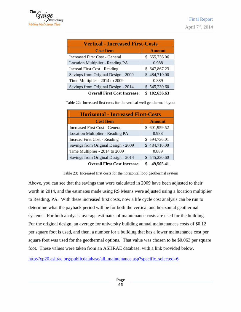
Final Report

April 7th, 2014

Page 65

Vertical - Increased First-Costs

Cost Item Amount

Increased First Cost - General $ 655,736.06

Location Multiplier - Reading PA 0.988

Incread First Cost - Reading $ 647,867.23

Savings from Original Design - 2009 $ 484,710.00

Time Multiplier - 2014 to 2009 0.889


Overall First Cost Increase: $ 102,636.63

Table 22: Increased first costs for the vertical well geothermal layout

Horizontal - Increased First-Costs

Cost Item Amount








Table 23: Increased first costs for the horizontal loop geothermal system

Above, you can see that the savings that were calculated in 2009 have been adjusted to their

worth in 2014, and the estimates made using RS Means were adjusted using a location multiplier

to Reading, PA. With these increased first costs, now a life cycle cost analysis can be run to

determine what the payback period will be for both the vertical and horizontal geothermal

systems. For both analysis, average estimates of maintenance costs are used for the building.

For the original design, an average for university building annual maintenances costs of $0.12

per square foot is used, and then, a number for a building that has a lower maintenance cost per

square foot was used for the geothermal options. That value was chosen to be $0.063 per square

foot. These values were taken from an ASHRAE database, with a link provided below.

http://xp20.ashrae.org/publicdatabase/all_maintenance.asp?specific_selected=6

http://xp20.ashrae.org/publicdatabase/all_maintenance.asp?specific_selected=6

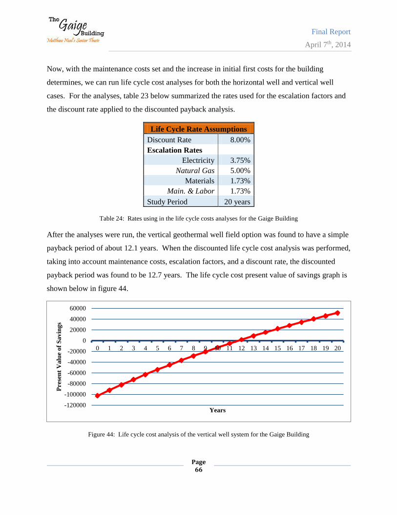
Final Report

April 7th, 2014

Page 66

Now, with the maintenance costs set and the increase in initial first costs for the building

determines, we can run life cycle cost analyses for both the horizontal well and vertical well

cases. For the analyses, table 23 below summarized the rates used for the escalation factors and

the discount rate applied to the discounted payback analysis.

Life Cycle Rate Assumptions

Discount Rate 8.00%

Escalation Rates

Electricity 3.75%

Natural Gas 5.00%

Materials 1.73%

Main. & Labor 1.73%

Study Period 20 years

Table 24: Rates using in the life cycle costs analyses for the Gaige Building

After the analyses were run, the vertical geothermal well field option was found to have a simple

payback period of about 12.1 years. When the discounted life cycle cost analysis was performed,

taking into account maintenance costs, escalation factors, and a discount rate, the discounted

payback period was found to be 12.7 years. The life cycle cost present value of savings graph is

shown below in figure 44.

Figure 44: Life cycle cost analysis of the vertical well system for the Gaige Building

-120000

-100000

-80000

-60000

-40000

-20000

0

20000

40000

60000

0 1 2 3 4 5 6 7 8 9 10 11 12 13 14 15 16 17 18 19 20

Pre

sen

t V

alu

e o

f S

av

ing

s

Years

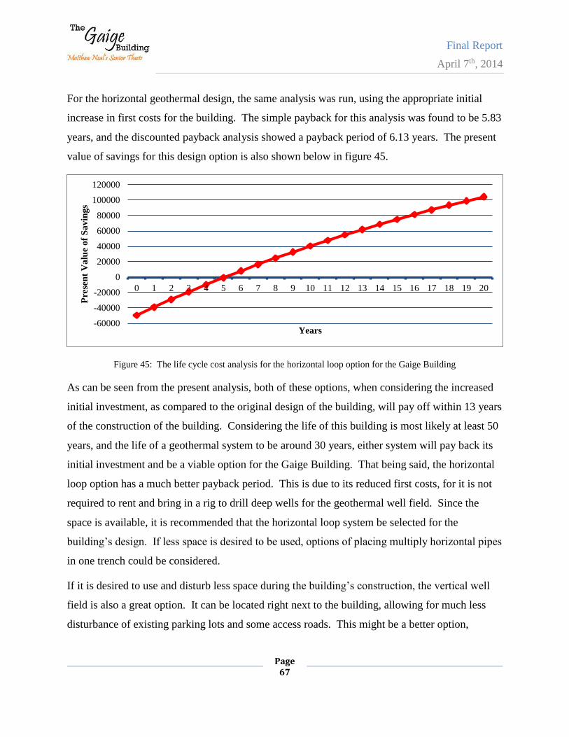
Final Report

April 7th, 2014

Page 67

For the horizontal geothermal design, the same analysis was run, using the appropriate initial

increase in first costs for the building. The simple payback for this analysis was found to be 5.83

years, and the discounted payback analysis showed a payback period of 6.13 years. The present

value of savings for this design option is also shown below in figure 45.

Figure 45: The life cycle cost analysis for the horizontal loop option for the Gaige Building

As can be seen from the present analysis, both of these options, when considering the increased

initial investment, as compared to the original design of the building, will pay off within 13 years

of the construction of the building. Considering the life of this building is most likely at least 50

years, and the life of a geothermal system to be around 30 years, either system will pay back its

initial investment and be a viable option for the Gaige Building. That being said, the horizontal

loop option has a much better payback period. This is due to its reduced first costs, for it is not

required to rent and bring in a rig to drill deep wells for the geothermal well field. Since the

space is available, it is recommended that the horizontal loop system be selected for the

building’s design. If less space is desired to be used, options of placing multiply horizontal pipes

in one trench could be considered.

If it is desired to use and disturb less space during the building’s construction, the vertical well

field is also a great option. It can be located right next to the building, allowing for much less

disturbance of existing parking lots and some access roads. This might be a better option,

-60000

-40000

-20000

0

20000

40000

60000

80000

100000

120000

0 1 2 3 4 5 6 7 8 9 10 11 12 13 14 15 16 17 18 19 20

Pre

sen

t V

alu

e o

f S

av

ing

s

Years

Final Report

April 7th, 2014

Page 68

depend upon whether or not the construction would take place during the school year when

classes are in session or not. Both design options are fine choices, and the decision would be left

to the owners to weigh out the pros and cons relating to the increased payback.

3.2: Campus-wide Geothermal System Analysis

After realizing the geothermal potential of the Reading, PA area, the idea of implementing a

geothermal system for the entire Berks campus was also an option that could be analyzed.

Toward the beginning of the project, I was provided with monthly billing data for all of the

campus buildings on the Penn State Berks campus. With this data available, a rough estimate of

how all of these building could work together, in one centralized system needed to be observed.

With the rare opportunity of having many buildings with the same owner so close to each other,

a centralized system needed to be analyzed.

3.2.1: Campus-wide Geothermal Motivation

Various factors influenced the motivation behind this analysis. First, it is known that whenever

you can produce energy at a centralized plant, you can do so much more efficiently than if you

are producing energy separately at many different sites with less efficient equipment. Also, for a

geothermal system, since it is already extremely energy efficient, allowing many different load

sources to take advantage of this efficiency would have great potential benefits. Also, the

potential load diversity that could be present on the campus seemed like a good option as well.

If all of the buildings were to be run off a centralized system, if certain buildings have very

difference schedules of loading, one building might experience maximum load a different time

than other buildings. Instead of having to size two systems separately at the separate maximum

loads, the two buildings energy sources could be combined, and great load diversity benefits

could be realized.

On the Penn State Berks campus, many different types of building exist: public assembly

spaces, classrooms, offices, dorm buildings, athletic facilities, and others. Along with all of

these buildings being located relatively near to each other, there is still a large amount of open

space available on the campus, which gives good potential to install geothermal well fields. If a

certain amount of load diversity could be realized, it would also decrease the number of wells

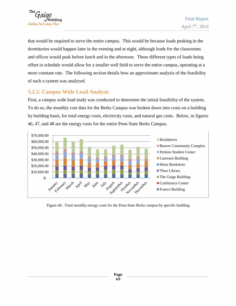
Final Report

April 7th, 2014

Page 69

that would be required to serve the entire campus. This would be because loads peaking in the

dormitories would happen later in the evening and at night, although loads for the classrooms

and offices would peak before lunch and in the afternoon. These different types of loads being

offset in schedule would allow for a smaller well field to serve the entire campus, operating at a

more constant rate. The following section details how an approximate analysis of the feasibility

of such a system was analyzed.

3.2.2: Campus Wide Load Analysis

First, a campus wide load study was conducted to determine the initial feasibility of the system.

To do so, the monthly cost data for the Berks Campus was broken down into costs on a building

by building basis, for total energy costs, electricity costs, and natural gas costs. Below, in figures

46, 47, and 48 are the energy costs for the entire Penn State Berks Campus.

Figure 46: Total monthly energy costs for the Penn State Berks campus by specific building

$-

$10,000.00

$20,000.00

$30,000.00

$40,000.00

$50,000.00

$60,000.00

$70,000.00Residences

Beaver Community Complex

Perkins Student Center

Luerssen Building

Hintz Bookstore

Thun Library

The Gaige Building

Conference Center

Franco Building

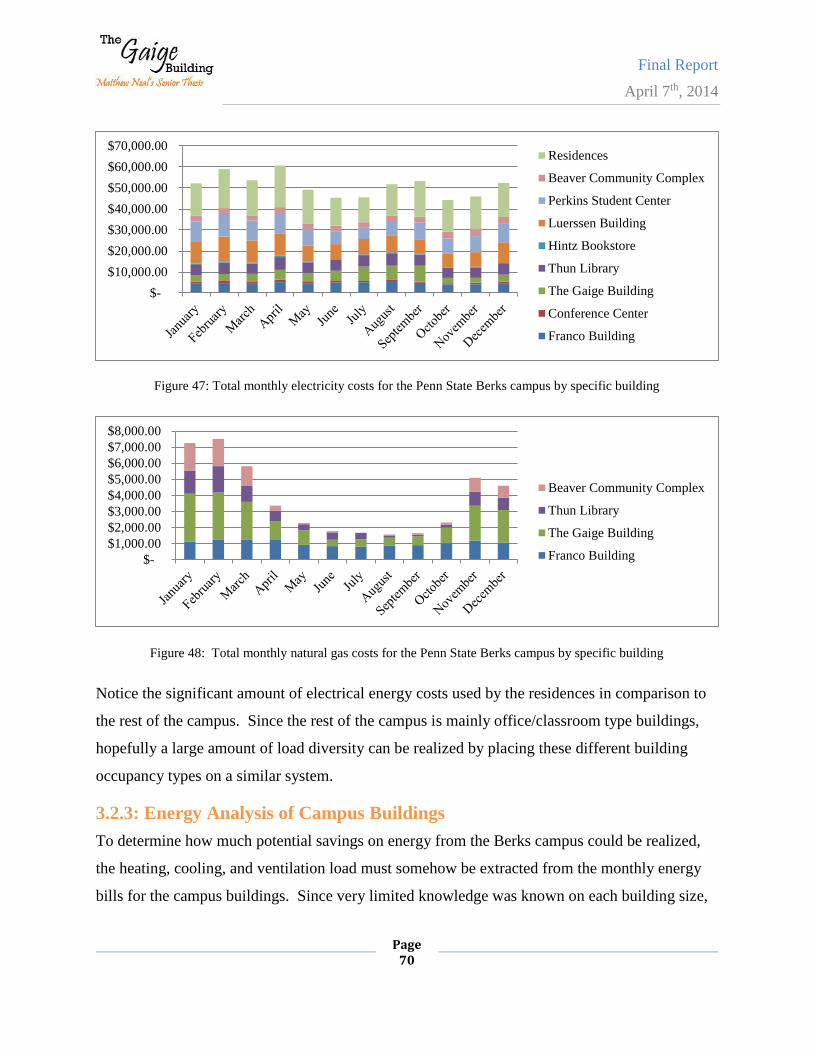
Final Report

April 7th, 2014

Page 70

Figure 47: Total monthly electricity costs for the Penn State Berks campus by specific building

Figure 48: Total monthly natural gas costs for the Penn State Berks campus by specific building

Notice the significant amount of electrical energy costs used by the residences in comparison to

the rest of the campus. Since the rest of the campus is mainly office/classroom type buildings,

hopefully a large amount of load diversity can be realized by placing these different building

occupancy types on a similar system.

3.2.3: Energy Analysis of Campus Buildings

To determine how much potential savings on energy from the Berks campus could be realized,

the heating, cooling, and ventilation load must somehow be extracted from the monthly energy

bills for the campus buildings. Since very limited knowledge was known on each building size,

$-

$10,000.00

$20,000.00

$30,000.00

$40,000.00

$50,000.00

$60,000.00

$70,000.00Residences


Perkins Student Center

Luerssen Building

Hintz Bookstore

Thun Library

The Gaige Building

Conference Center

Franco Building

$-

$1,000.00

$2,000.00

$3,000.00

$4,000.00

$5,000.00

$6,000.00

$7,000.00

$8,000.00


Thun Library

The Gaige Building

Franco Building

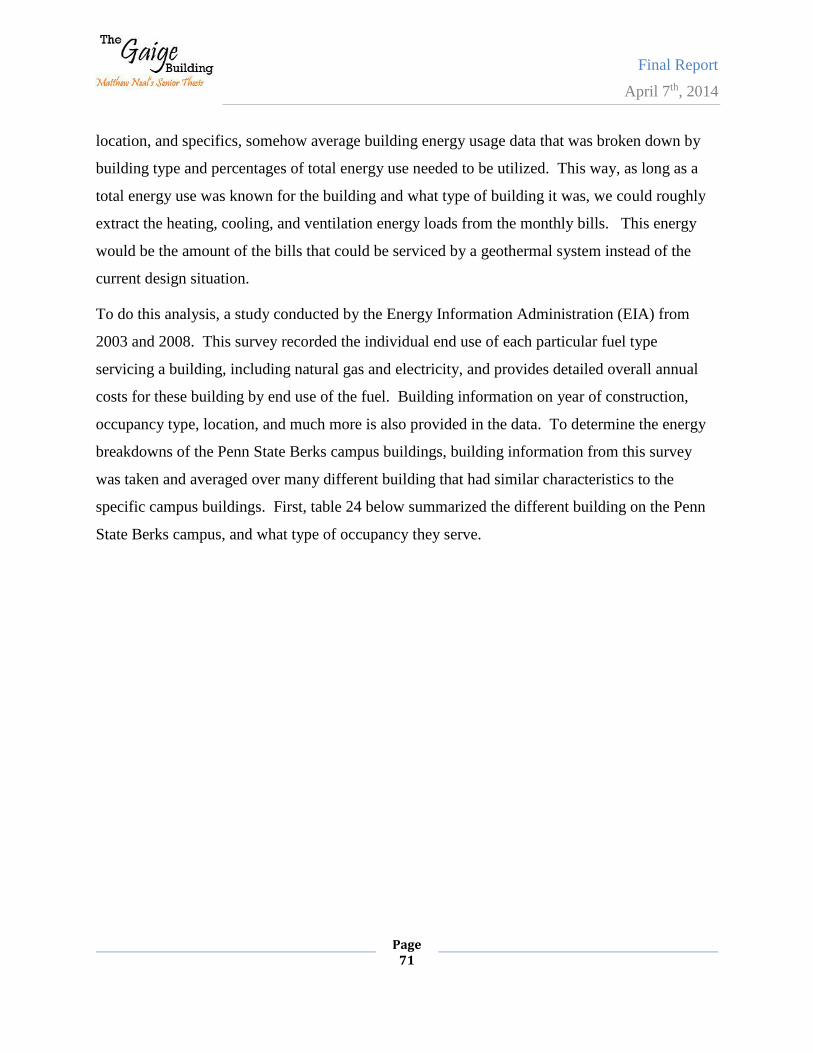
Final Report

April 7th, 2014

Page 71

location, and specifics, somehow average building energy usage data that was broken down by

building type and percentages of total energy use needed to be utilized. This way, as long as a

total energy use was known for the building and what type of building it was, we could roughly

extract the heating, cooling, and ventilation energy loads from the monthly bills. This energy

would be the amount of the bills that could be serviced by a geothermal system instead of the

current design situation.

To do this analysis, a study conducted by the Energy Information Administration (EIA) from

2003 and 2008. This survey recorded the individual end use of each particular fuel type

servicing a building, including natural gas and electricity, and provides detailed overall annual

costs for these building by end use of the fuel. Building information on year of construction,

occupancy type, location, and much more is also provided in the data. To determine the energy

breakdowns of the Penn State Berks campus buildings, building information from this survey

was taken and averaged over many different building that had similar characteristics to the

specific campus buildings. First, table 24 below summarized the different building on the Penn

State Berks campus, and what type of occupancy they serve.

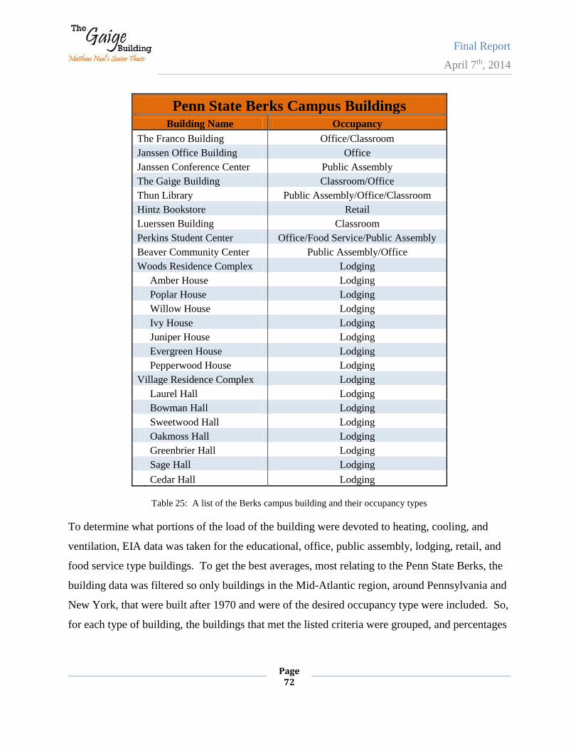
Final Report

April 7th, 2014

Page 72

Penn State Berks Campus Buildings Building Name Occupancy

The Franco Building Office/Classroom

Janssen Office Building Office

Janssen Conference Center Public Assembly

The Gaige Building Classroom/Office

Thun Library Public Assembly/Office/Classroom

Hintz Bookstore Retail

Luerssen Building Classroom

Perkins Student Center Office/Food Service/Public Assembly

Beaver Community Center Public Assembly/Office

Woods Residence Complex Lodging

Amber House Lodging

Poplar House Lodging

Willow House Lodging

Ivy House Lodging

Juniper House Lodging

Evergreen House Lodging

Pepperwood House Lodging

Village Residence Complex Lodging

Laurel Hall Lodging

Bowman Hall Lodging

Sweetwood Hall Lodging

Oakmoss Hall Lodging

Greenbrier Hall Lodging

Sage Hall Lodging

Cedar Hall Lodging

Table 25: A list of the Berks campus building and their occupancy types

To determine what portions of the load of the building were devoted to heating, cooling, and

ventilation, EIA data was taken for the educational, office, public assembly, lodging, retail, and

food service type buildings. To get the best averages, most relating to the Penn State Berks, the

building data was filtered so only buildings in the Mid-Atlantic region, around Pennsylvania and

New York, that were built after 1970 and were of the desired occupancy type were included. So,

for each type of building, the buildings that met the listed criteria were grouped, and percentages

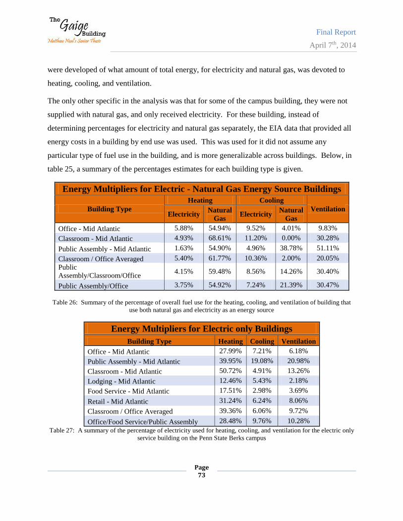
Final Report

April 7th, 2014

Page 73

were developed of what amount of total energy, for electricity and natural gas, was devoted to

heating, cooling, and ventilation.

The only other specific in the analysis was that for some of the campus building, they were not

supplied with natural gas, and only received electricity. For these building, instead of

determining percentages for electricity and natural gas separately, the EIA data that provided all

energy costs in a building by end use was used. This was used for it did not assume any

particular type of fuel use in the building, and is more generalizable across buildings. Below, in

table 25, a summary of the percentages estimates for each building type is given.

Energy Multipliers for Electric - Natural Gas Energy Source Buildings

Building Type

Heating Cooling

Ventilation Electricity

Natural

Gas Electricity

Natural

Gas

Office - Mid Atlantic 5.88% 54.94% 9.52% 4.01% 9.83%

Classroom - Mid Atlantic 4.93% 68.61% 11.20% 0.00% 30.28%

Public Assembly - Mid Atlantic 1.63% 54.90% 4.96% 38.78% 51.11%

Classroom / Office Averaged 5.40% 61.77% 10.36% 2.00% 20.05%

Public

Assembly/Classroom/Office 4.15% 59.48% 8.56% 14.26% 30.40%

Public Assembly/Office 3.75% 54.92% 7.24% 21.39% 30.47%

Table 26: Summary of the percentage of overall fuel use for the heating, cooling, and ventilation of building that

use both natural gas and electricity as an energy source

Energy Multipliers for Electric only Buildings

Building Type Heating Cooling Ventilation

Office - Mid Atlantic 27.99% 7.21% 6.18%

Public Assembly - Mid Atlantic 39.95% 19.08% 20.98%

Classroom - Mid Atlantic 50.72% 4.91% 13.26%

Lodging - Mid Atlantic 12.46% 5.43% 2.18%

Food Service - Mid Atlantic 17.51% 2.98% 3.69%

Retail - Mid Atlantic 31.24% 6.24% 8.06%

Classroom / Office Averaged 39.36% 6.06% 9.72%

Office/Food Service/Public Assembly 28.48% 9.76% 10.28%

Table 27: A summary of the percentage of electricity used for heating, cooling, and ventilation for the electric only

service building on the Penn State Berks campus

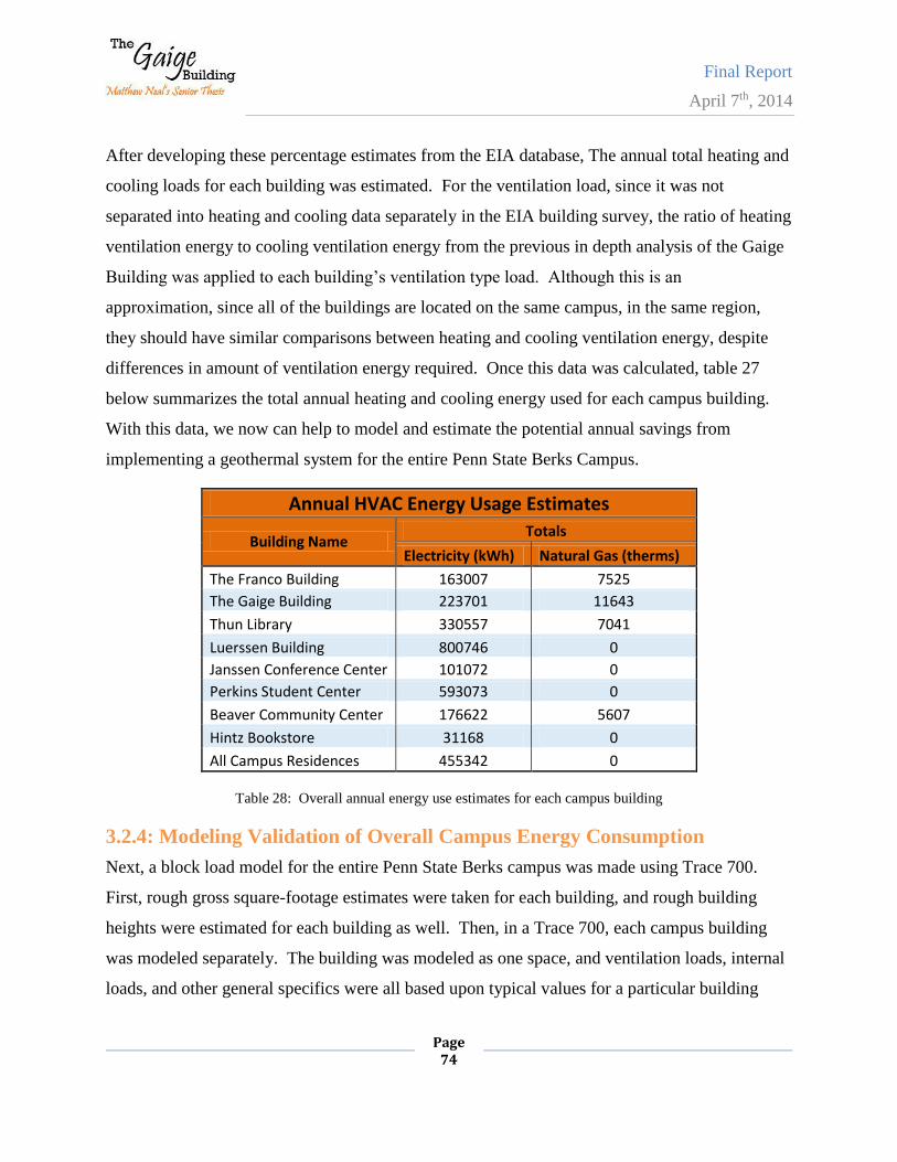
Final Report

April 7th, 2014

Page 74

After developing these percentage estimates from the EIA database, The annual total heating and

cooling loads for each building was estimated. For the ventilation load, since it was not

separated into heating and cooling data separately in the EIA building survey, the ratio of heating

ventilation energy to cooling ventilation energy from the previous in depth analysis of the Gaige

Building was applied to each building’s ventilation type load. Although this is an

approximation, since all of the buildings are located on the same campus, in the same region,

they should have similar comparisons between heating and cooling ventilation energy, despite

differences in amount of ventilation energy required. Once this data was calculated, table 27

below summarizes the total annual heating and cooling energy used for each campus building.

With this data, we now can help to model and estimate the potential annual savings from

implementing a geothermal system for the entire Penn State Berks Campus.

Annual HVAC Energy Usage Estimates

Building Name Totals

Electricity (kWh) Natural Gas (therms)

The Franco Building 163007 7525

The Gaige Building 223701 11643

Thun Library 330557 7041

Luerssen Building 800746 0

Janssen Conference Center 101072 0

Perkins Student Center 593073 0

Beaver Community Center 176622 5607

Hintz Bookstore 31168 0

All Campus Residences 455342 0

Table 28: Overall annual energy use estimates for each campus building

3.2.4: Modeling Validation of Overall Campus Energy Consumption

Next, a block load model for the entire Penn State Berks campus was made using Trace 700.

First, rough gross square-footage estimates were taken for each building, and rough building

heights were estimated for each building as well. Then, in a Trace 700, each campus building

was modeled separately. The building was modeled as one space, and ventilation loads, internal

loads, and other general specifics were all based upon typical values for a particular building

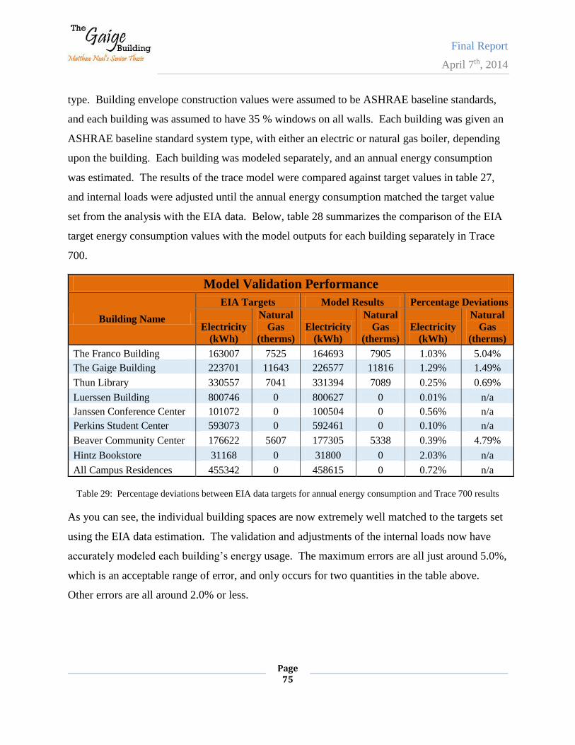
Final Report

April 7th, 2014

Page 75

type. Building envelope construction values were assumed to be ASHRAE baseline standards,

and each building was assumed to have 35 % windows on all walls. Each building was given an

ASHRAE baseline standard system type, with either an electric or natural gas boiler, depending

upon the building. Each building was modeled separately, and an annual energy consumption

was estimated. The results of the trace model were compared against target values in table 27,

and internal loads were adjusted until the annual energy consumption matched the target value

set from the analysis with the EIA data. Below, table 28 summarizes the comparison of the EIA

target energy consumption values with the model outputs for each building separately in Trace

700.

Model Validation Performance

Building Name

EIA Targets Model Results Percentage Deviations

Electricity

(kWh)

Natural

Gas

(therms)

Electricity

(kWh)

Natural

Gas

(therms)

Electricity

(kWh)

Natural

Gas

(therms)

The Franco Building 163007 7525 164693 7905 1.03% 5.04%

The Gaige Building 223701 11643 226577 11816 1.29% 1.49%

Thun Library 330557 7041 331394 7089 0.25% 0.69%

Luerssen Building 800746 0 800627 0 0.01% n/a

Janssen Conference Center 101072 0 100504 0 0.56% n/a

Perkins Student Center 593073 0 592461 0 0.10% n/a

Beaver Community Center 176622 5607 177305 5338 0.39% 4.79%

Hintz Bookstore 31168 0 31800 0 2.03% n/a

All Campus Residences 455342 0 458615 0 0.72% n/a

Table 29: Percentage deviations between EIA data targets for annual energy consumption and Trace 700 results

As you can see, the individual building spaces are now extremely well matched to the targets set

using the EIA data estimation. The validation and adjustments of the internal loads now have

accurately modeled each building’s energy usage. The maximum errors are all just around 5.0%,

which is an acceptable range of error, and only occurs for two quantities in the table above.

Other errors are all around 2.0% or less.

Final Report

April 7th, 2014

Page 76

3.2.5: Geothermal Modeling of Overall Campus

Now that a model of each campus building has been created and validated, a Trace model of the

entire campus needs to be created. For this model, each building that was modeled separately in

the prior analysis were all combined into one Trace 700 model. For the purposes of this analysis,

each building is treated as a ‘room’ in the buildings are then all able to be connected to the same

central system. Again, the trace models for the buildings only contain HVAC loads and energy

uses. All other loads, such as receptacle and other miscellaneous loads have been removed from

the model for simplicity in model comparison and validation. First, all of the buildings were

added together, and two systems were created for the model. One was packaged rooftop unit

system with a gas fired boiler, and the other was a packaged rooftop unit system with electric

resistance heating. The buildings were then assigned to the system that was representative of

their current system. From this, energy rates were given, and total annual energy cost estimates

were extracted.

After this new ‘baseline’ model was created, the model was copied, and the system servicing the

campus was changed. The system was altered to a ground loop source that was serviced by

water source heat pumps. The number of water source heat pump assigned to each building wa

determined using data from the Gaige Building’s analysis. The total number of heat pumps in

the Gaige Building was divided by the cooling load of the Gaige Building, provided a heat

pumps per ton of cooling fraction. Then, this fraction was simply multiplied peak cooling loads

of each of the building to determine the number of heat pumps that should be assigned to each

building. Finally, the model of the entire campus, now on a solely geothermal system was run.

Below, figure 49 summaries the comparison between monthly costs of the entire campus on its

current system and using a potentially full geothermal system. Overall, an annual energy savings

of $58,166.00, which will go toward paying off the initial increased costs of the system.

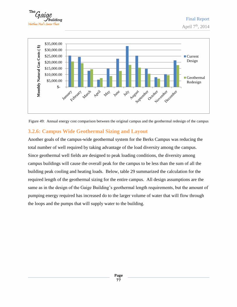
Final Report

April 7th, 2014

Page 77

Figure 49: Annual energy cost comparison between the original campus and the geothermal redesign of the campus

3.2.6: Campus Wide Geothermal Sizing and Layout

Another goals of the campus-wide geothermal system for the Berks Campus was reducing the

total number of well required by taking advantage of the load diversity among the campus.

Since geothermal well fields are designed to peak loading conditions, the diversity among

campus buildings will cause the overall peak for the campus to be less than the sum of all the

building peak cooling and heating loads. Below, table 29 summarized the calculation for the

required length of the geothermal sizing for the entire campus. All design assumptions are the

same as in the design of the Gaige Building’s geothermal length requirements, but the amount of

pumping energy required has increased do to the larger volume of water that will flow through

the loops and the pumps that will supply water to the building.

$-

$5,000.00

$10,000.00

$15,000.00

$20,000.00

$25,000.00

$30,000.00

$35,000.00

Mo

nth

ly N

atu

ral

Ga

s C

ost

s (

$)

Current

Design

Geothermal

Redesign

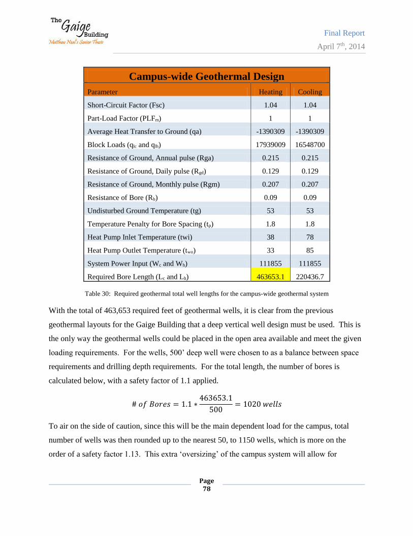
Final Report

April 7th, 2014

Page 78

Campus-wide Geothermal Design

Parameter Heating Cooling

Short-Circuit Factor (Fsc) 1.04 1.04

Part-Load Factor (PLFm) 1 1

Average Heat Transfer to Ground (qa) -1390309 -1390309

Block Loads (qlc and qlh) 17939009 16548700

Resistance of Ground, Annual pulse (Rga) 0.215 0.215

Resistance of Ground, Daily pulse (Rgd) 0.129 0.129

Resistance of Ground, Monthly pulse (Rgm) 0.207 0.207

Resistance of Bore (Rb) 0.09 0.09

Undisturbed Ground Temperature (tg) 53 53

Temperature Penalty for Bore Spacing (tp) 1.8 1.8

Heat Pump Inlet Temperature (twi) 38 78

Heat Pump Outlet Temperature (two) 33 85

System Power Input (Wc and Wh) 111855 111855

Required Bore Length (Lc and Lh) 463653.1 220436.7

Table 30: Required geothermal total well lengths for the campus-wide geothermal system

With the total of 463,653 required feet of geothermal wells, it is clear from the previous

geothermal layouts for the Gaige Building that a deep vertical well design must be used. This is

the only way the geothermal wells could be placed in the open area available and meet the given

loading requirements. For the wells, 500’ deep well were chosen to as a balance between space

requirements and drilling depth requirements. For the total length, the number of bores is

calculated below, with a safety factor of 1.1 applied.

# 𝑜𝑓 𝐵𝑜𝑟𝑒𝑠 = 1.1 ∗463653.1

500= 1020 𝑤𝑒𝑙𝑙𝑠

To air on the side of caution, since this will be the main dependent load for the campus, total

number of wells was then rounded up to the nearest 50, to 1150 wells, which is more on the

order of a safety factor 1.13. This extra ‘oversizing’ of the campus system will allow for

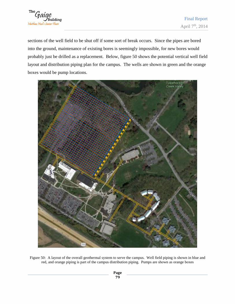
Final Report

April 7th, 2014

Page 79

sections of the well field to be shut off if some sort of break occurs. Since the pipes are bored

into the ground, maintenance of existing bores is seemingly impossible, for new bores would

probably just be drilled as a replacement. Below, figure 50 shows the potential vertical well field

layout and distribution piping plan for the campus. The wells are shown in green and the orange

boxes would be pump locations.

Figure 50: A layout of the overall geothermal system to serve the campus. Well field piping is shown in blue and

red, and orange piping is part of the campus distribution piping. Pumps are shown as orange boxes

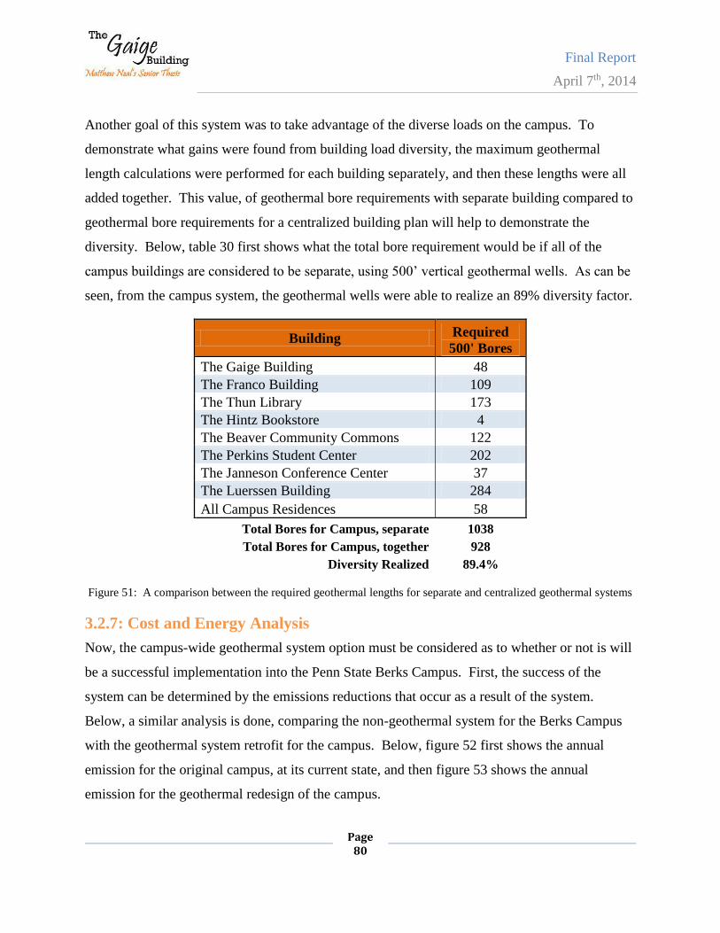
Final Report

April 7th, 2014

Page 80

Another goal of this system was to take advantage of the diverse loads on the campus. To

demonstrate what gains were found from building load diversity, the maximum geothermal

length calculations were performed for each building separately, and then these lengths were all

added together. This value, of geothermal bore requirements with separate building compared to

geothermal bore requirements for a centralized building plan will help to demonstrate the

diversity. Below, table 30 first shows what the total bore requirement would be if all of the

campus buildings are considered to be separate, using 500’ vertical geothermal wells. As can be

seen, from the campus system, the geothermal wells were able to realize an 89% diversity factor.

Building Required

500' Bores

The Gaige Building 48

The Franco Building 109

The Thun Library 173

The Hintz Bookstore 4

The Beaver Community Commons 122

The Perkins Student Center 202

The Janneson Conference Center 37

The Luerssen Building 284

All Campus Residences 58

Total Bores for Campus, separate 1038

Total Bores for Campus, together 928

Diversity Realized 89.4%

Figure 51: A comparison between the required geothermal lengths for separate and centralized geothermal systems

3.2.7: Cost and Energy Analysis

Now, the campus-wide geothermal system option must be considered as to whether or not is will

be a successful implementation into the Penn State Berks Campus. First, the success of the

system can be determined by the emissions reductions that occur as a result of the system.

Below, a similar analysis is done, comparing the non-geothermal system for the Berks Campus

with the geothermal system retrofit for the campus. Below, figure 52 first shows the annual

emission for the original campus, at its current state, and then figure 53 shows the annual

emission for the geothermal redesign of the campus.

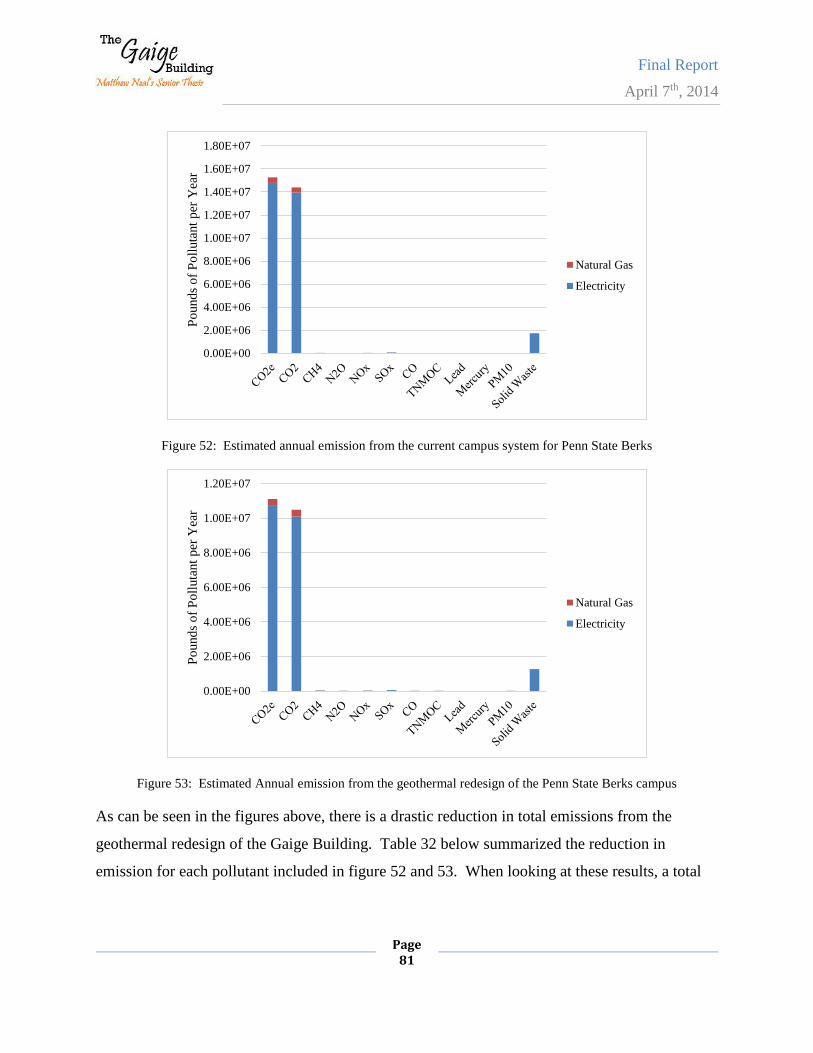
Final Report

April 7th, 2014

Page 81

Figure 52: Estimated annual emission from the current campus system for Penn State Berks

Figure 53: Estimated Annual emission from the geothermal redesign of the Penn State Berks campus

As can be seen in the figures above, there is a drastic reduction in total emissions from the

geothermal redesign of the Gaige Building. Table 32 below summarized the reduction in

emission for each pollutant included in figure 52 and 53. When looking at these results, a total

0.00E+00

2.00E+06

4.00E+06

6.00E+06

8.00E+06

1.00E+07

1.20E+07

1.40E+07

1.60E+07

1.80E+07

Po

und

s o

f P

oll

uta

nt

per

Yea

r

Natural Gas

Electricity

0.00E+00

2.00E+06

4.00E+06

6.00E+06

8.00E+06

1.00E+07

1.20E+07

Po

und

s o

f P

oll

uta

nt

per

Yea

r

Natural Gas

Electricity

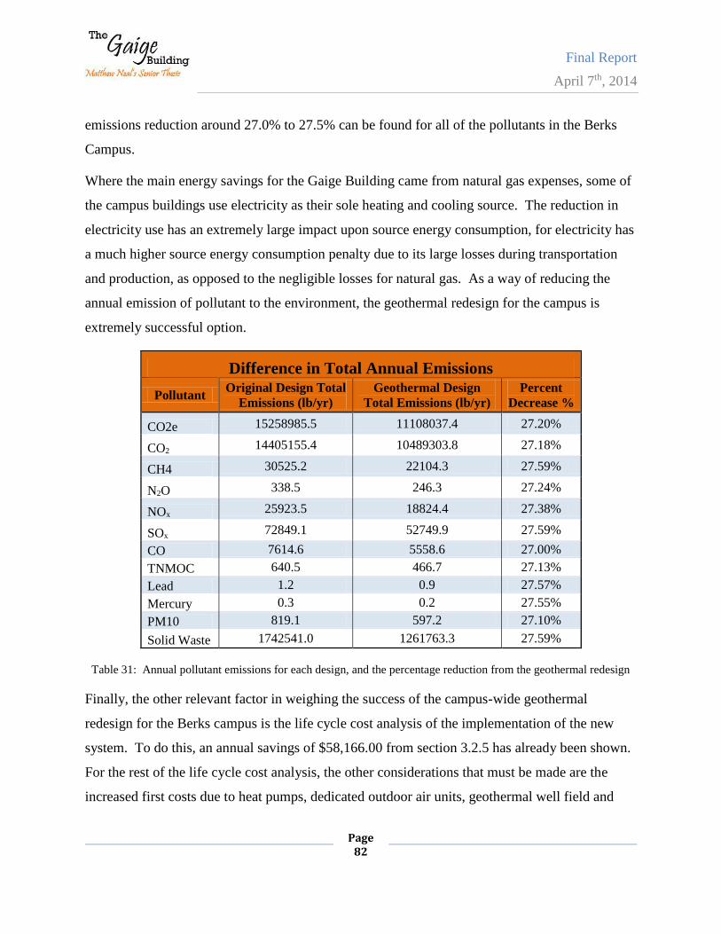
Final Report

April 7th, 2014

Page 82

emissions reduction around 27.0% to 27.5% can be found for all of the pollutants in the Berks

Campus.

Where the main energy savings for the Gaige Building came from natural gas expenses, some of

the campus buildings use electricity as their sole heating and cooling source. The reduction in

electricity use has an extremely large impact upon source energy consumption, for electricity has

a much higher source energy consumption penalty due to its large losses during transportation

and production, as opposed to the negligible losses for natural gas. As a way of reducing the

annual emission of pollutant to the environment, the geothermal redesign for the campus is

extremely successful option.

Difference in Total Annual Emissions

Pollutant Original Design Total

Emissions (lb/yr)

Geothermal Design

Total Emissions (lb/yr)

Percent

Decrease %

CO2e 15258985.5 11108037.4 27.20%

CO2 14405155.4 10489303.8 27.18%

CH4 30525.2 22104.3 27.59%

N2O 338.5 246.3 27.24%

NOx 25923.5 18824.4 27.38%

SOx 72849.1 52749.9 27.59%

CO 7614.6 5558.6 27.00%

TNMOC 640.5 466.7 27.13%

Lead 1.2 0.9 27.57%

Mercury 0.3 0.2 27.55%

PM10 819.1 597.2 27.10%

Solid Waste 1742541.0 1261763.3 27.59%

Table 31: Annual pollutant emissions for each design, and the percentage reduction from the geothermal redesign

Finally, the other relevant factor in weighing the success of the campus-wide geothermal

redesign for the Berks campus is the life cycle cost analysis of the implementation of the new

system. To do this, an annual savings of $58,166.00 from section 3.2.5 has already been shown.

For the rest of the life cycle cost analysis, the other considerations that must be made are the

increased first costs due to heat pumps, dedicated outdoor air units, geothermal well field and

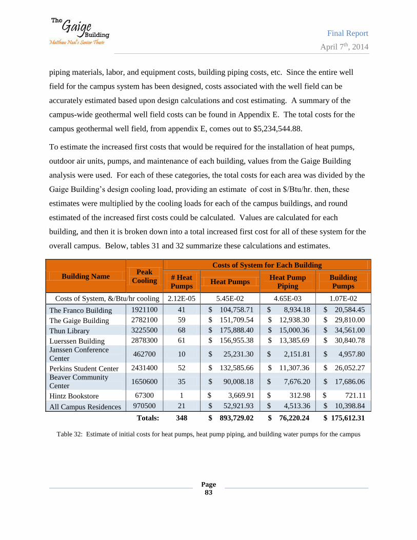
Final Report

April 7th, 2014

Page 83

piping materials, labor, and equipment costs, building piping costs, etc. Since the entire well

field for the campus system has been designed, costs associated with the well field can be

accurately estimated based upon design calculations and cost estimating. A summary of the

campus-wide geothermal well field costs can be found in Appendix E. The total costs for the

campus geothermal well field, from appendix E, comes out to $5,234,544.88.

To estimate the increased first costs that would be required for the installation of heat pumps,

outdoor air units, pumps, and maintenance of each building, values from the Gaige Building

analysis were used. For each of these categories, the total costs for each area was divided by the

Gaige Building’s design cooling load, providing an estimate of cost in $/Btu/hr. then, these

estimates were multiplied by the cooling loads for each of the campus buildings, and round

estimated of the increased first costs could be calculated. Values are calculated for each

building, and then it is broken down into a total increased first cost for all of these system for the

overall campus. Below, tables 31 and 32 summarize these calculations and estimates.

Building Name Peak

Cooling

Costs of System for Each Building

# Heat

Pumps Heat Pumps

Heat Pump

Piping

Building

Pumps

Costs of System, &/Btu/hr cooling 2.12E-05 5.45E-02 4.65E-03 1.07E-02

The Franco Building 1921100 41 $ 104,758.71 $ 8,934.18 $ 20,584.45

The Gaige Building 2782100 59 $ 151,709.54 $ 12,938.30 $ 29,810.00

Thun Library 3225500 68 $ 175,888.40 $ 15,000.36 $ 34,561.00

Luerssen Building 2878300 61 $ 156,955.38 $ 13,385.69 $ 30,840.78

Janssen Conference

Center 462700 10 $ 25,231.30 $ 2,151.81 $ 4,957.80

Perkins Student Center 2431400 52 $ 132,585.66 $ 11,307.36 $ 26,052.27

Beaver Community

Center 1650600 35 $ 90,008.18 $ 7,676.20 $ 17,686.06

Hintz Bookstore 67300 1 $ 3,669.91 $ 312.98 $ 721.11

All Campus Residences 970500 21 $ 52,921.93 $ 4,513.36 $ 10,398.84

Totals: 348 $ 893,729.02 $ 76,220.24 $ 175,612.31

Table 32: Estimate of initial costs for heat pumps, heat pump piping, and building water pumps for the campus

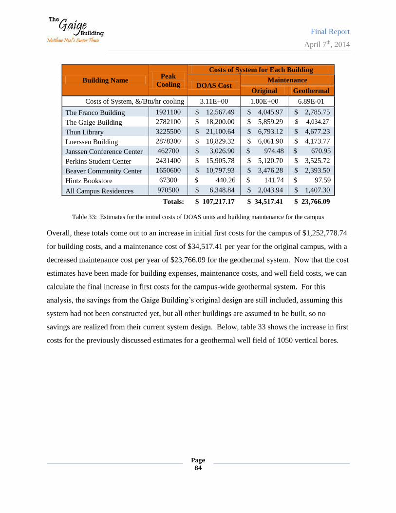
Final Report

April 7th, 2014

Page 84

Building Name Peak

Cooling

Costs of System for Each Building

DOAS Cost Maintenance

Original Geothermal

Costs of System, &/Btu/hr cooling 3.11E+00 1.00E+00 6.89E-01

The Franco Building 1921100 $ 12,567.49 $ 4,045.97 $ 2,785.75

The Gaige Building 2782100 $ 18,200.00 $ 5,859.29 $ 4,034.27

Thun Library 3225500 $ 21,100.64 $ 6,793.12 $ 4,677.23

Luerssen Building 2878300 $ 18,829.32 $ 6,061.90 $ 4,173.77

Janssen Conference Center 462700 $ 3,026.90 $ 974.48 $ 670.95

Perkins Student Center 2431400 $ 15,905.78 $ 5,120.70 $ 3,525.72

Beaver Community Center 1650600 $ 10,797.93 $ 3,476.28 $ 2,393.50

Hintz Bookstore 67300 $ 440.26 $ 141.74 $ 97.59

All Campus Residences 970500 $ 6,348.84 $ 2,043.94 $ 1,407.30

Totals: $ 107,217.17 $ 34,517.41 $ 23,766.09

Table 33: Estimates for the initial costs of DOAS units and building maintenance for the campus

Overall, these totals come out to an increase in initial first costs for the campus of $1,252,778.74

for building costs, and a maintenance cost of $34,517.41 per year for the original campus, with a

decreased maintenance cost per year of $23,766.09 for the geothermal system. Now that the cost

estimates have been made for building expenses, maintenance costs, and well field costs, we can

calculate the final increase in first costs for the campus-wide geothermal system. For this

analysis, the savings from the Gaige Building’s original design are still included, assuming this

system had not been constructed yet, but all other buildings are assumed to be built, so no

savings are realized from their current system design. Below, table 33 shows the increase in first

costs for the previously discussed estimates for a geothermal well field of 1050 vertical bores.

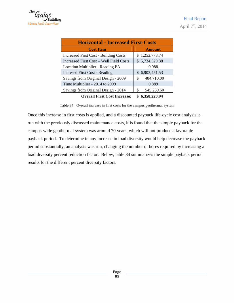
Final Report

April 7th, 2014

Page 85


Cost Item Amount

Increased First Cost - Building Costs $ 1,252,778.74

Increased First Cost – Well Field Costs $ 5,734,520.38


Incresed First Cost - Reading $ 6,903,451.53




Overall First Cost Increase: $ 6,358,220.94

Table 34: Overall increase in first costs for the campus geothermal system

Once this increase in first costs is applied, and a discounted payback life-cycle cost analysis is

run with the previously discussed maintenance costs, it is found that the simple payback for the

campus-wide geothermal system was around 70 years, which will not produce a favorable

payback period. To determine in any increase in load diversity would help decrease the payback

period substantially, an analysis was run, changing the number of bores required by increasing a

load diversity percent reduction factor. Below, table 34 summarizes the simple payback period

results for the different percent diversity factors.

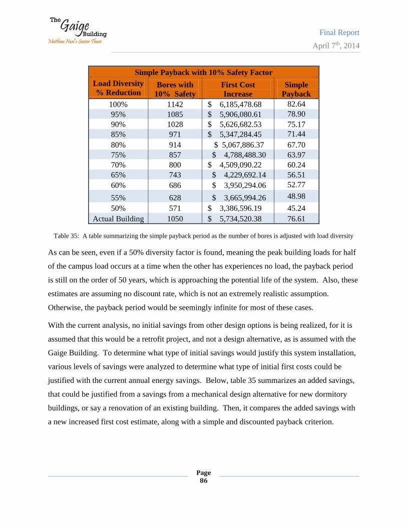
Final Report

April 7th, 2014

Page 86

Simple Payback with 10% Safety Factor

Load Diversity

% Reduction Bores with

10% Safety

First Cost

Increase

Simple

Payback

100% 1142 $ 6,185,478.68 82.64

95% 1085 $ 5,906,080.61 78.90

90% 1028 $ 5,626,682.53 75.17

85% 971 $ 5,347,284.45 71.44

80% 914 $ 5,067,886.37 67.70

75% 857 $ 4,788,488.30 63.97

70% 800 $ 4,509,090.22 60.24

65% 743 $ 4,229,692.14 56.51

60% 686 $ 3,950,294.06 52.77

55% 628 $ 3,665,994.26 48.98

50% 571 $ 3,386,596.19 45.24

Actual Building 1050 $ 5,734,520.38 76.61

Table 35: A table summarizing the simple payback period as the number of bores is adjusted with load diversity

As can be seen, even if a 50% diversity factor is found, meaning the peak building loads for half

of the campus load occurs at a time when the other has experiences no load, the payback period

is still on the order of 50 years, which is approaching the potential life of the system. Also, these

estimates are assuming no discount rate, which is not an extremely realistic assumption.

Otherwise, the payback period would be seemingly infinite for most of these cases.

With the current analysis, no initial savings from other design options is being realized, for it is

assumed that this would be a retrofit project, and not a design alternative, as is assumed with the

Gaige Building. To determine what type of initial savings would justify this system installation,

various levels of savings were analyzed to determine what type of initial first costs could be

justified with the current annual energy savings. Below, table 35 summarizes an added savings,

that could be justified from a savings from a mechanical design alternative for new dormitory

buildings, or say a renovation of an existing building. Then, it compares the added savings with

a new increased first cost estimate, along with a simple and discounted payback criterion.

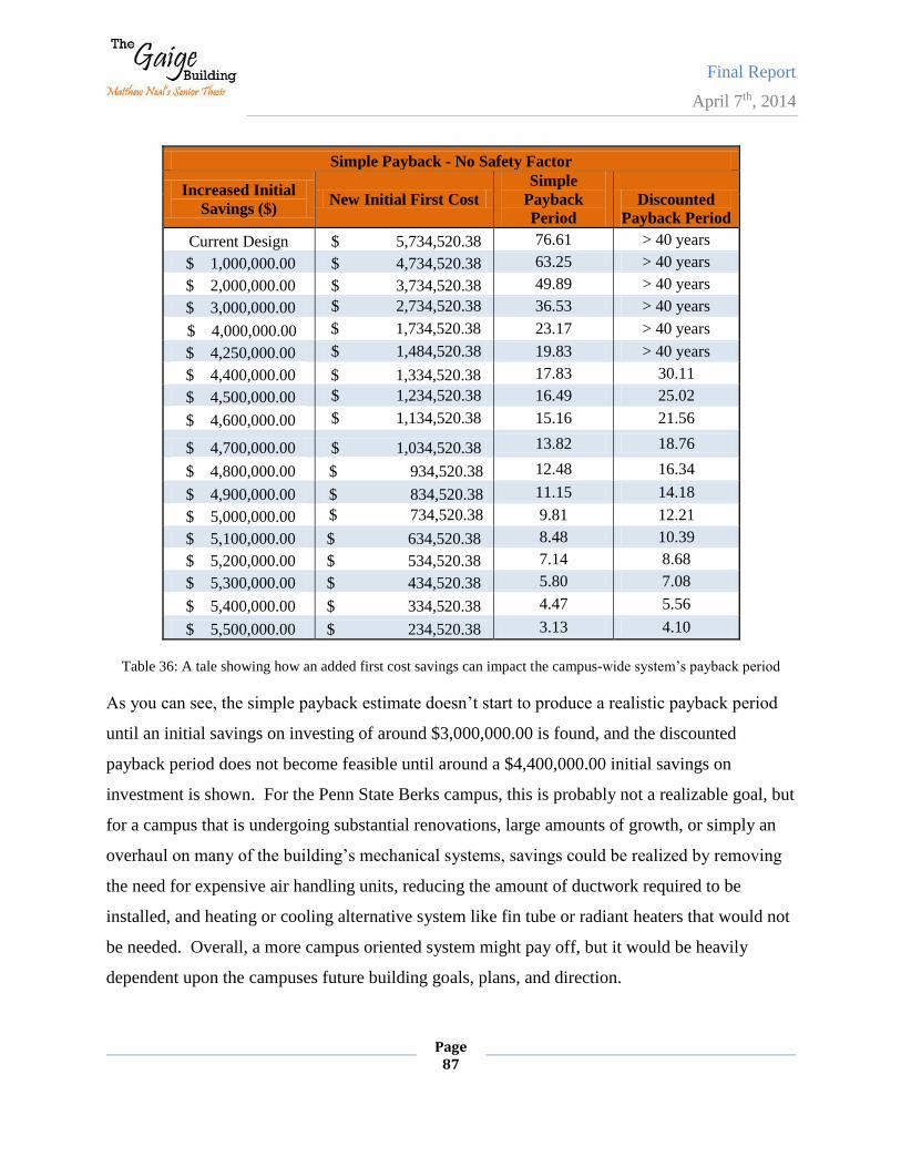
Final Report

April 7th, 2014

Page 87

Simple Payback - No Safety Factor

Increased Initial

Savings ($) New Initial First Cost

Simple

Payback

Period

Discounted

Payback Period

Current Design $ 5,734,520.38 76.61 > 40 years

$ 1,000,000.00 $ 4,734,520.38 63.25 > 40 years

$ 2,000,000.00 $ 3,734,520.38 49.89 > 40 years

$ 3,000,000.00 $ 2,734,520.38 36.53 > 40 years

$ 4,000,000.00 $ 1,734,520.38 23.17 > 40 years

$ 4,250,000.00 $ 1,484,520.38 19.83 > 40 years

$ 4,400,000.00 $ 1,334,520.38 17.83 30.11

$ 4,500,000.00 $ 1,234,520.38 16.49 25.02

$ 4,600,000.00 $ 1,134,520.38 15.16 21.56

$ 4,700,000.00 $ 1,034,520.38 13.82 18.76

$ 4,800,000.00 $ 934,520.38 12.48 16.34

$ 4,900,000.00 $ 834,520.38 11.15 14.18

$ 5,000,000.00 $ 734,520.38 9.81 12.21

$ 5,100,000.00 $ 634,520.38 8.48 10.39

$ 5,200,000.00 $ 534,520.38 7.14 8.68

$ 5,300,000.00 $ 434,520.38 5.80 7.08

$ 5,400,000.00 $ 334,520.38 4.47 5.56

$ 5,500,000.00 $ 234,520.38 3.13 4.10

Table 36: A tale showing how an added first cost savings can impact the campus-wide system’s payback period

As you can see, the simple payback estimate doesn’t start to produce a realistic payback period

until an initial savings on investing of around $3,000,000.00 is found, and the discounted

payback period does not become feasible until around a $4,400,000.00 initial savings on

investment is shown. For the Penn State Berks campus, this is probably not a realizable goal, but

for a campus that is undergoing substantial renovations, large amounts of growth, or simply an

overhaul on many of the building’s mechanical systems, savings could be realized by removing

the need for expensive air handling units, reducing the amount of ductwork required to be

installed, and heating or cooling alternative system like fin tube or radiant heaters that would not

be needed. Overall, a more campus oriented system might pay off, but it would be heavily

dependent upon the campuses future building goals, plans, and direction.

Final Report

April 7th, 2014

Page 88

Chapter 4: Acoustical Breadth

In order to consider how the new geothermal system would impact the acoustic performance of

the Gaige Building, an acoustical analysis was performed. In this analysis, heat pump locations

were modeled in a room acoustics program call ODEON. This program allows a user to model

room geometries, assign material properties to surfaces, specify transmission loss values to room

partitions, place sound sources within rooms, and place receivers in the rooms as well. ODEON

was used to determine how specific heat pump placements impacted the background noise within

the classroom spaces they were serving. Also, since this thesis is selected to count as an honors

thesis, it was decided to add an additional analysis to this breadth to justify the thesis as an

honors thesis as well. For this, a measurement trip was taken to the Gaige Building, and onsite

measurements were taken for the room acoustics parameters of reverberation time, background

noise level, and transmission loss for various classrooms and conference rooms.

4.1: Honors Work: Acoustics Performance of the Gaige Building

The main goal of this measurement trip was to provide a learning experience for myself and to

determine the overall acoustic performance of the Gaige Building, with respect to the classroom

acoustics standard, ANSI S12.60, put forth through the American national Standards Institute in

conjunction with the Acoustical Society of America. Also, I asked a few members of the first

architectural acoustics class, AE 309, if they wanted to join me on the trip. Two students went

on this trip, and had a great opportunity to become exposed to acoustic measurement techniques

for architectural acoustics. As well, they had a chance to apply the knowledge they were

learning in AE 309 outside of the classroom, which is not typically possible in the field of

architectural acoustics through Penn State’s AE program.

4.1.1: Room Acoustics Performance

The Classroom acoustics standard, ANSI S12.60, is a standard set forth that specifies various

acoustical design requirements for classroom. The basis of the standard is for K-12 classrooms,

and it provided recommended reverberation time (RT) set points and minimum background noise

level (BNL) requirements. Although the Gaige Building is not a K-12 classroom space, these

values are still good design targets, and the performance of the classroom should be reasonable

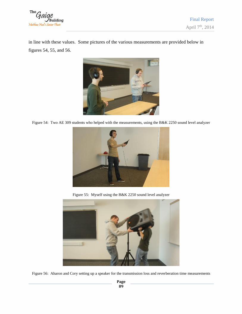
Final Report

April 7th, 2014

Page 89

in line with these values. Some pictures of the various measurements are provided below in

figures 54, 55, and 56.

Figure 54: Two AE 309 students who helped with the measurements, using the B&K 2250 sound level analyzer

Figure 55: Myself using the B&K 2250 sound level analyzer

Figure 56: Aharon and Cory setting up a speaker for the transmission loss and reverberation time measurements

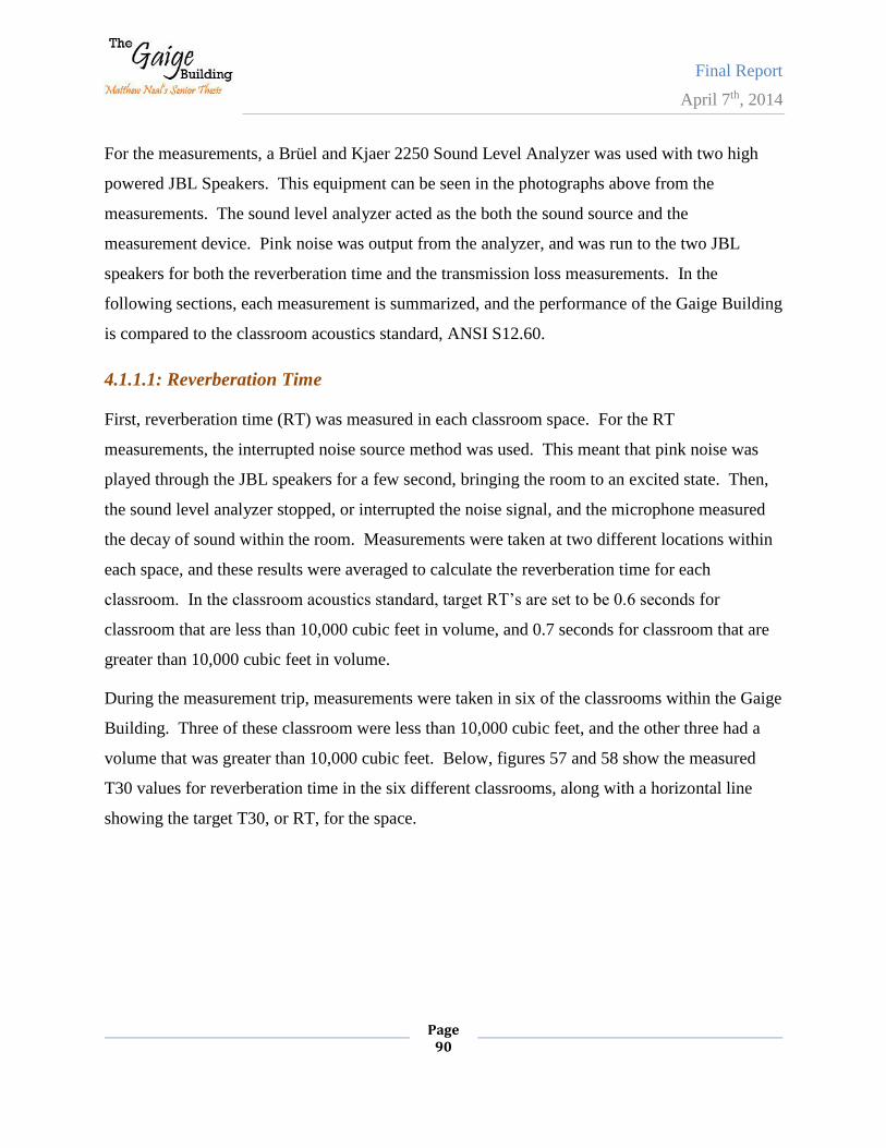
Final Report

April 7th, 2014

Page 90

For the measurements, a Brüel and Kjaer 2250 Sound Level Analyzer was used with two high

powered JBL Speakers. This equipment can be seen in the photographs above from the

measurements. The sound level analyzer acted as the both the sound source and the

measurement device. Pink noise was output from the analyzer, and was run to the two JBL

speakers for both the reverberation time and the transmission loss measurements. In the

following sections, each measurement is summarized, and the performance of the Gaige Building

is compared to the classroom acoustics standard, ANSI S12.60.

4.1.1.1: Reverberation Time

First, reverberation time (RT) was measured in each classroom space. For the RT

measurements, the interrupted noise source method was used. This meant that pink noise was

played through the JBL speakers for a few second, bringing the room to an excited state. Then,

the sound level analyzer stopped, or interrupted the noise signal, and the microphone measured

the decay of sound within the room. Measurements were taken at two different locations within

each space, and these results were averaged to calculate the reverberation time for each

classroom. In the classroom acoustics standard, target RT’s are set to be 0.6 seconds for

classroom that are less than 10,000 cubic feet in volume, and 0.7 seconds for classroom that are

greater than 10,000 cubic feet in volume.

During the measurement trip, measurements were taken in six of the classrooms within the Gaige

Building. Three of these classroom were less than 10,000 cubic feet, and the other three had a

volume that was greater than 10,000 cubic feet. Below, figures 57 and 58 show the measured

T30 values for reverberation time in the six different classrooms, along with a horizontal line

showing the target T30, or RT, for the space.

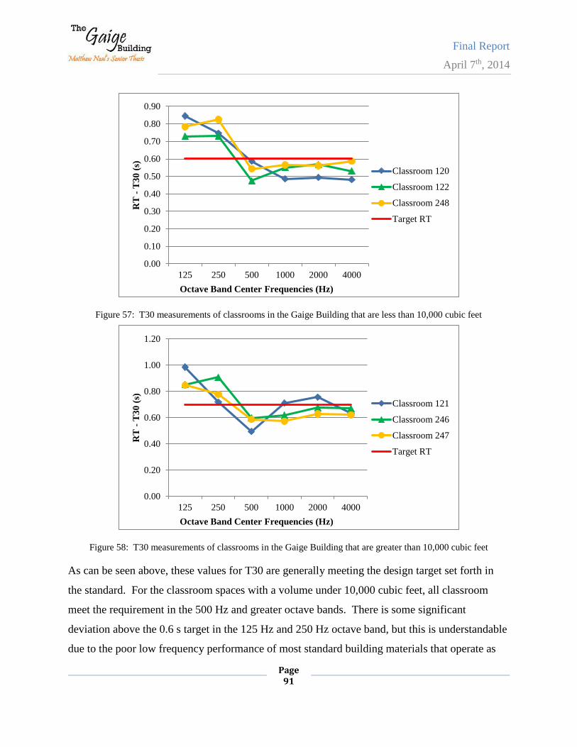
Final Report

April 7th, 2014

Page 91

Figure 57: T30 measurements of classrooms in the Gaige Building that are less than 10,000 cubic feet

Figure 58: T30 measurements of classrooms in the Gaige Building that are greater than 10,000 cubic feet

As can be seen above, these values for T30 are generally meeting the design target set forth in

the standard. For the classroom spaces with a volume under 10,000 cubic feet, all classroom

meet the requirement in the 500 Hz and greater octave bands. There is some significant

deviation above the 0.6 s target in the 125 Hz and 250 Hz octave band, but this is understandable

due to the poor low frequency performance of most standard building materials that operate as

0.00

0.10

0.20

0.30

0.40

0.50

0.60

0.70

0.80

0.90

125 250 500 1000 2000 4000

RT

-T

30

(s)

Octave Band Center Frequencies (Hz)

Classroom 120

Classroom 122

Classroom 248

Target RT

0.00

0.20

0.40

0.60

0.80

1.00

1.20

125 250 500 1000 2000 4000

RT

-T

30

(s)

Octave Band Center Frequencies (Hz)

Classroom 121

Classroom 246

Classroom 247

Target RT

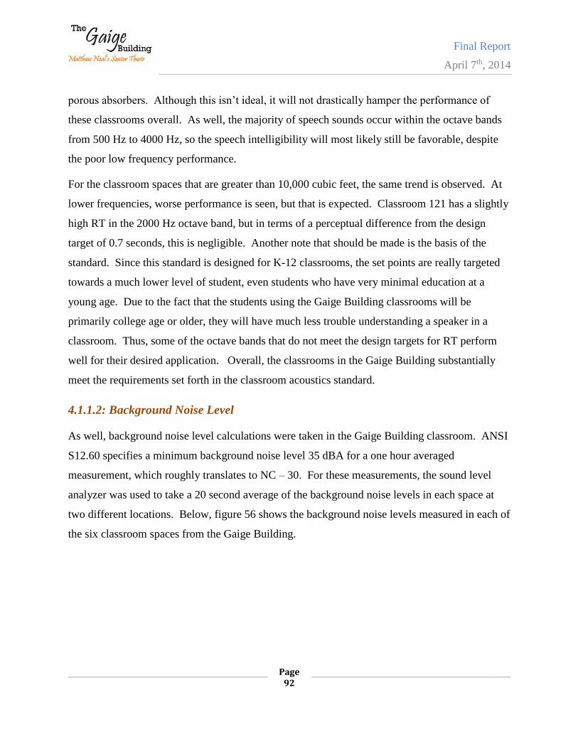
Final Report

April 7th, 2014

Page 92

porous absorbers. Although this isn’t ideal, it will not drastically hamper the performance of

these classrooms overall. As well, the majority of speech sounds occur within the octave bands

from 500 Hz to 4000 Hz, so the speech intelligibility will most likely still be favorable, despite

the poor low frequency performance.

For the classroom spaces that are greater than 10,000 cubic feet, the same trend is observed. At

lower frequencies, worse performance is seen, but that is expected. Classroom 121 has a slightly

high RT in the 2000 Hz octave band, but in terms of a perceptual difference from the design

target of 0.7 seconds, this is negligible. Another note that should be made is the basis of the

standard. Since this standard is designed for K-12 classrooms, the set points are really targeted

towards a much lower level of student, even students who have very minimal education at a

young age. Due to the fact that the students using the Gaige Building classrooms will be

primarily college age or older, they will have much less trouble understanding a speaker in a

classroom. Thus, some of the octave bands that do not meet the design targets for RT perform

well for their desired application. Overall, the classrooms in the Gaige Building substantially

meet the requirements set forth in the classroom acoustics standard.

4.1.1.2: Background Noise Level

As well, background noise level calculations were taken in the Gaige Building classroom. ANSI

S12.60 specifies a minimum background noise level 35 dBA for a one hour averaged

measurement, which roughly translates to NC – 30. For these measurements, the sound level

analyzer was used to take a 20 second average of the background noise levels in each space at

two different locations. Below, figure 56 shows the background noise levels measured in each of

the six classroom spaces from the Gaige Building.

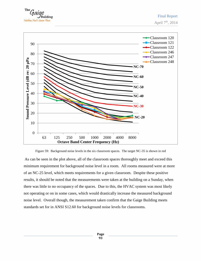
Final Report

April 7th, 2014

Page 93

Figure 59: Background noise levels in the six classroom spaces. The target NC-35 is shown in red

As can be seen in the plot above, all of the classroom spaces thoroughly meet and exceed this

minimum requirement for background noise level in a room. All rooms measured were at more

of an NC-25 level, which meets requirements for a given classroom. Despite these positive

results, it should be noted that the measurements were taken at the building on a Sunday, when

there was little to no occupancy of the spaces. Due to this, the HVAC system was most likely

not operating or on in some cases, which would drastically increase the measured background

noise level. Overall though, the measurement taken confirm that the Gaige Building meets

standards set for in ANSI S12.60 for background noise levels for classrooms.

0

10

20

30

40

50

60

70

80

90

63 125 250 500 1000 2000 4000 8000

Sou

nd

Pre

ssu

re L

evel

(d

B r

e: 2

0 µ

Pa

Octave Band Center Frequency (Hz)

Classroom 120

Classroom 121

Classroom 122

Classroom 246

Classroom 247

Classroom 248

NC-70

NC-60

NC-50

NC-40

NC-30

NC-20

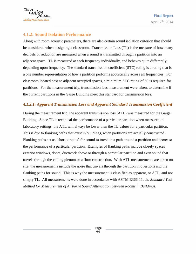
Final Report

April 7th, 2014

Page 94

4.1.2: Sound Isolation Performance

Along with room acoustic parameters, there are also certain sound isolation criterion that should

be considered when designing a classroom. Transmission Loss (TL) is the measure of how many

decibels of reduction are measured when a sound is transmitted through a partition into an

adjacent space. TL is measured at each frequency individually, and behaves quite differently,

depending upon frequency. The standard transmission coefficient (STC) rating is a rating that is

a one number representation of how a partition performs acoustically across all frequencies. For

classroom located next to adjacent occupied spaces, a minimum STC rating of 50 is required for

partitions. For the measurement trip, transmission loss measurement were taken, to determine if

the current partitions in the Gaige Building meet this standard for transmission loss.

4.1.2.1: Apparent Transmission Loss and Apparent Standard Transmission Coefficient

During the measurement trip, the apparent transmission loss (ATL) was measured for the Gaige

Building. Since TL is technical the performance of a particular partition when measured in

laboratory settings, the ATL will always be lower than the TL values for a particular partition.

This is due to flanking paths that exist in buildings, when partitions are actually constructed.

Flanking paths act as ‘short-circuits’ for sound to travel in a path around a partition and decrease

the performance of a particular partition. Examples of flanking paths include closely spaces

exterior windows, doors, ductwork above or through a particular partition and even sound that

travels through the ceiling plenum or a floor construction. With ATL measurements are taken on

site, the measurements include the noise that travels through the partition in questions and the

flanking paths for sound. This is why the measurement is classified as apparent, or ATL, and not

simply TL. All measurements were done in accordance with ASTM E366-11, the Standard Test

Method for Measurement of Airborne Sound Attenuation between Rooms in Buildings.

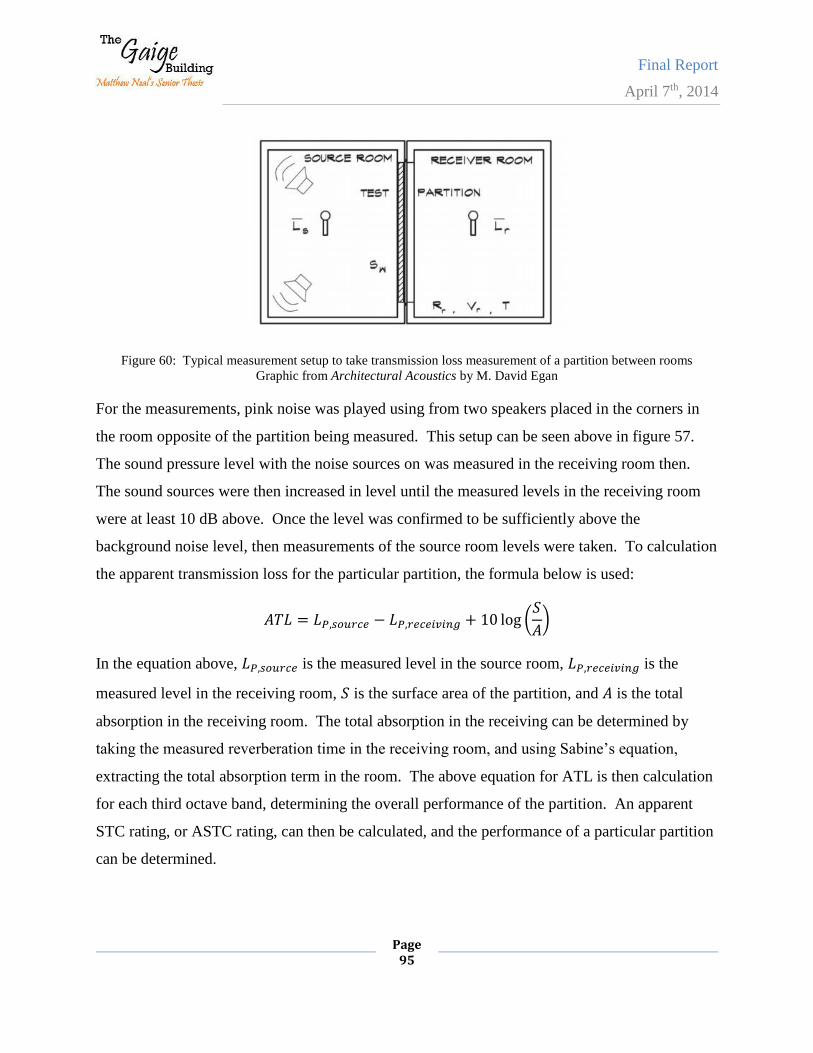
Final Report

April 7th, 2014

Page 95

Figure 60: Typical measurement setup to take transmission loss measurement of a partition between rooms

Graphic from Architectural Acoustics by M. David Egan

For the measurements, pink noise was played using from two speakers placed in the corners in

the room opposite of the partition being measured. This setup can be seen above in figure 57.

The sound pressure level with the noise sources on was measured in the receiving room then.

The sound sources were then increased in level until the measured levels in the receiving room

were at least 10 dB above. Once the level was confirmed to be sufficiently above the

background noise level, then measurements of the source room levels were taken. To calculation

the apparent transmission loss for the particular partition, the formula below is used:

𝐴𝑇𝐿 = 𝐿𝑃,𝑠𝑜𝑢𝑟𝑐𝑒 − 𝐿𝑃,𝑟𝑒𝑐𝑒𝑖𝑣𝑖𝑛𝑔 + 10 log (𝑆

𝐴)

In the equation above, 𝐿𝑃,𝑠𝑜𝑢𝑟𝑐𝑒 is the measured level in the source room, 𝐿𝑃,𝑟𝑒𝑐𝑒𝑖𝑣𝑖𝑛𝑔 is the

measured level in the receiving room, 𝑆 is the surface area of the partition, and 𝐴 is the total

absorption in the receiving room. The total absorption in the receiving can be determined by

taking the measured reverberation time in the receiving room, and using Sabine’s equation,

extracting the total absorption term in the room. The above equation for ATL is then calculation

for each third octave band, determining the overall performance of the partition. An apparent

STC rating, or ASTC rating, can then be calculated, and the performance of a particular partition

can be determined.

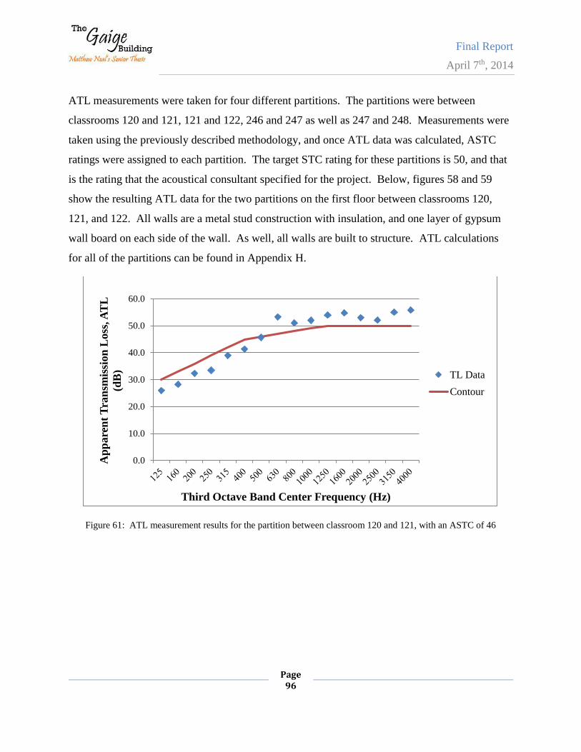
Final Report

April 7th, 2014

Page 96

ATL measurements were taken for four different partitions. The partitions were between

classrooms 120 and 121, 121 and 122, 246 and 247 as well as 247 and 248. Measurements were

taken using the previously described methodology, and once ATL data was calculated, ASTC

ratings were assigned to each partition. The target STC rating for these partitions is 50, and that

is the rating that the acoustical consultant specified for the project. Below, figures 58 and 59

show the resulting ATL data for the two partitions on the first floor between classrooms 120,

121, and 122. All walls are a metal stud construction with insulation, and one layer of gypsum

wall board on each side of the wall. As well, all walls are built to structure. ATL calculations

for all of the partitions can be found in Appendix H.

Figure 61: ATL measurement results for the partition between classroom 120 and 121, with an ASTC of 46

0.0

10.0

20.0

30.0

40.0

50.0

60.0

Ap

pare

nt

Tra

nsm

issi

on

Loss

, AT

L

(dB

)

Third Octave Band Center Frequency (Hz)

TL Data

Contour

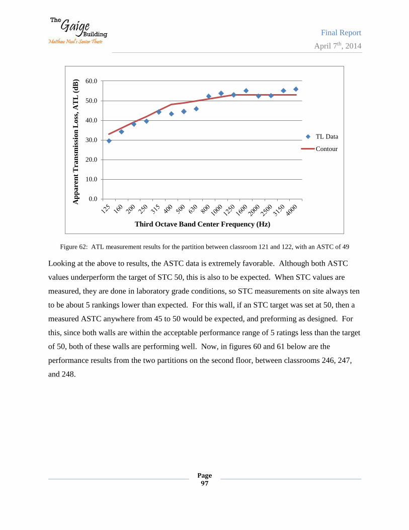
Final Report

April 7th, 2014

Page 97


Looking at the above to results, the ASTC data is extremely favorable. Although both ASTC

values underperform the target of STC 50, this is also to be expected. When STC values are

measured, they are done in laboratory grade conditions, so STC measurements on site always ten

to be about 5 rankings lower than expected. For this wall, if an STC target was set at 50, then a

measured ASTC anywhere from 45 to 50 would be expected, and preforming as designed. For

this, since both walls are within the acceptable performance range of 5 ratings less than the target

of 50, both of these walls are performing well. Now, in figures 60 and 61 below are the

performance results from the two partitions on the second floor, between classrooms 246, 247,

and 248.

0.0

10.0

20.0

30.0

40.0

50.0

60.0A

pp

are

nt

Tra

nsm

issi

on

Lo

ss,

AT

L (

dB

)


TL Data

Contour

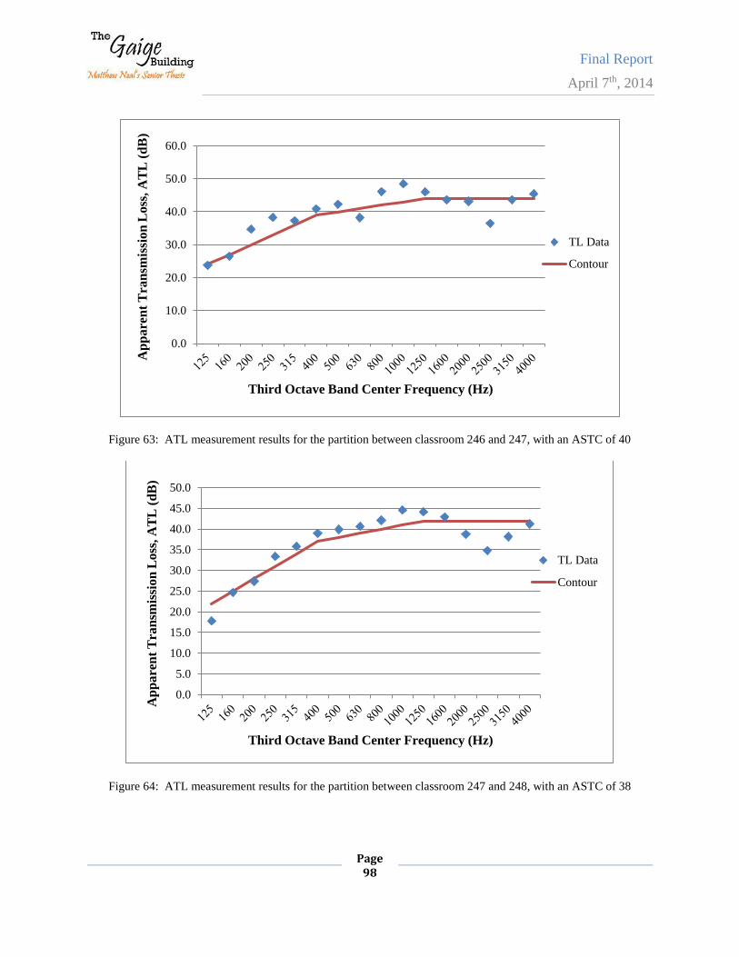
Final Report

April 7th, 2014

Page 98



0.0

10.0

20.0

30.0

40.0

50.0

60.0A

pp

are

nt

Tra

nsm

issi

on

Lo

ss,

AT

L (

dB

)


TL Data

Contour

0.0

5.0

10.0

15.0

20.0

25.0

30.0

35.0

40.0

45.0

50.0

Ap

pare

nt

Tra

nsm

issi

on

Lo

ss, A

TL

(d

B)


TL Data

Contour

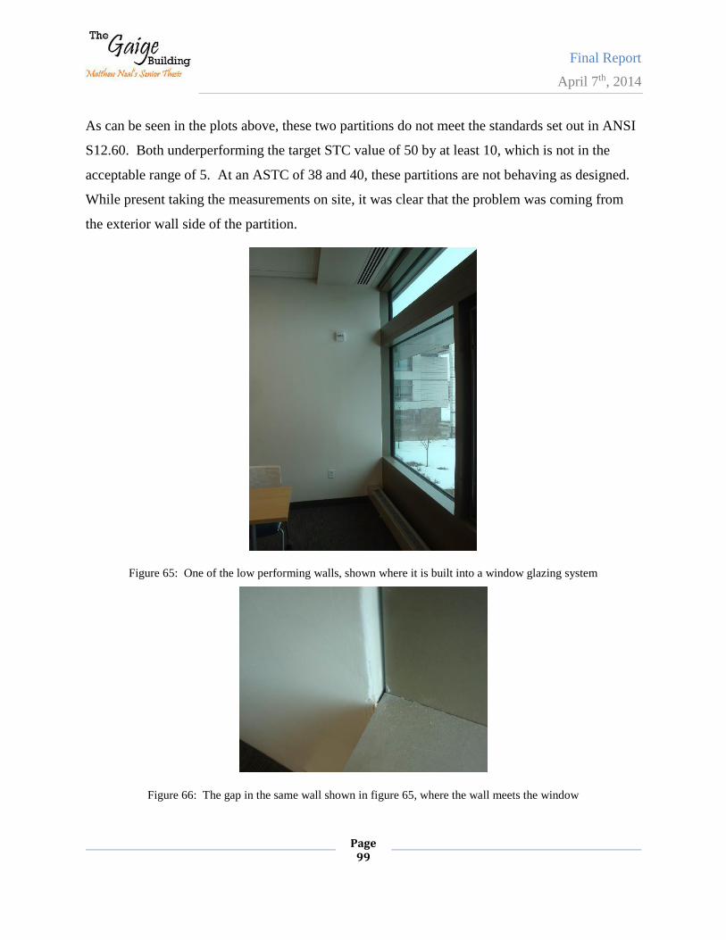
Final Report

April 7th, 2014

Page 99

As can be seen in the plots above, these two partitions do not meet the standards set out in ANSI

S12.60. Both underperforming the target STC value of 50 by at least 10, which is not in the

acceptable range of 5. At an ASTC of 38 and 40, these partitions are not behaving as designed.

While present taking the measurements on site, it was clear that the problem was coming from

the exterior wall side of the partition.

Figure 65: One of the low performing walls, shown where it is built into a window glazing system

Figure 66: The gap in the same wall shown in figure 65, where the wall meets the window

Final Report

April 7th, 2014

Page 100

The walls were built into a continuous glazing system, shown in figure 65 above, which ran

along the exterior of all of the classroom. Due to this, the walls were built very close up to the

windows, but they were not properly sealed, causing a huge decrease in acoustic performance.

The gap in the wall can also be seen in figure 66 above. As well, you can see a large dip present

in the TL measurements around the 2500 Hz third octave band. This could be some sort of

coincidence dip in the partition, or it could also be some sort of resonance that is happening due

to the sizing and spacing of the gap between the windows and the wall.

Anytime a hole exists in a building structure, it will behave like a ‘short-circuit’, just like a

flanking path, and drastically reduce the STC rating of any construction. Even if the opening is

small, it will still have a large effect on the performance of the partition. It is important to not

only specify acoustical caulking and sealant on a project, but also to be sure the installers know

that all openings and joints need to be well sealed, without any gaps or openings. Figure 62

below shows a picture of the wall overall, being built into the structure, and figure 63 shows the

small opening and gap between the walls and the windows.

As well, aural simulations, or auralizations were created showing what it would sound like if you

were sitting in the back of an classroom with a speaker talking on the other side of the wall in an

adjacent classroom. Auralizaitons were created in ODEON, a room acoustics modeling

software. These auralizaitons were made using the measured ATL data for the ASTC 38 wall

and the ASTC 49 wall, to help demonstrate the difference in performance. To listen to these

auralizations, please visit the acoustics page on my senior thesis CPEP website.

4.2: Heat Pump Noise Control and Isolation

Since the mechanical system of the Gaige Building is proposed to change to geothermal system,

as opposed to the standard rooftop unit system, various acoustical considerations must be made.

In a geothermal system that utilizes water source heat pumps, water from the group loop is piped

throughout the building using large capacity centrifugal pumps located in a mechanical room

where the ground loop enters the building. Then, that group loop is piped to each individual

water source heat pump. Each water source heat pump serves one room, or multiple smaller

rooms. Due to this change, the mechanical equipment now must be located within close

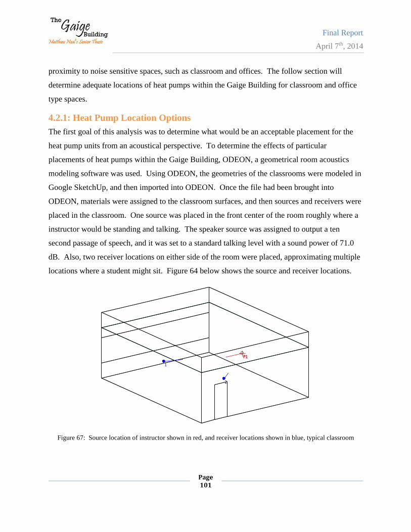
Final Report

April 7th, 2014

Page 101

proximity to noise sensitive spaces, such as classroom and offices. The follow section will

determine adequate locations of heat pumps within the Gaige Building for classroom and office

type spaces.

4.2.1: Heat Pump Location Options

The first goal of this analysis was to determine what would be an acceptable placement for the

heat pump units from an acoustical perspective. To determine the effects of particular

placements of heat pumps within the Gaige Building, ODEON, a geometrical room acoustics

modeling software was used. Using ODEON, the geometries of the classrooms were modeled in

Google SketchUp, and then imported into ODEON. Once the file had been brought into

ODEON, materials were assigned to the classroom surfaces, and then sources and receivers were

placed in the classroom. One source was placed in the front center of the room roughly where a

instructor would be standing and talking. The speaker source was assigned to output a ten

second passage of speech, and it was set to a standard talking level with a sound power of 71.0

dB. Also, two receiver locations on either side of the room were placed, approximating multiple

locations where a student might sit. Figure 64 below shows the source and receiver locations.

Figure 67: Source location of instructor shown in red, and receiver locations shown in blue, typical classroom

O

XY

Z

0 2 4 6 8 10 12 14 16 18 20 22 24 26 metres

0

2

4

6

8

10

12 metres

P1

1

2

P1

Odeon©1985-2013 Licensed to: Penn State University, USA Restricted version - research and teaching only!

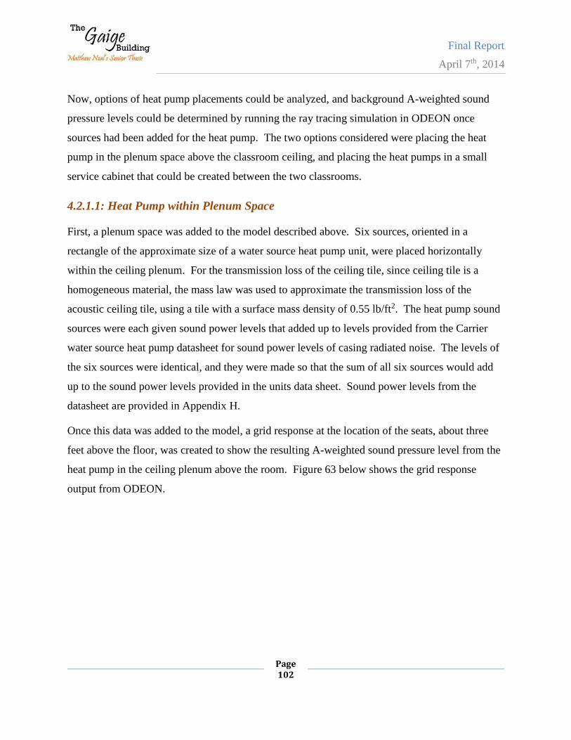
Final Report

April 7th, 2014

Page 102

Now, options of heat pump placements could be analyzed, and background A-weighted sound

pressure levels could be determined by running the ray tracing simulation in ODEON once

sources had been added for the heat pump. The two options considered were placing the heat

pump in the plenum space above the classroom ceiling, and placing the heat pumps in a small

service cabinet that could be created between the two classrooms.

4.2.1.1: Heat Pump within Plenum Space

First, a plenum space was added to the model described above. Six sources, oriented in a

rectangle of the approximate size of a water source heat pump unit, were placed horizontally

within the ceiling plenum. For the transmission loss of the ceiling tile, since ceiling tile is a

homogeneous material, the mass law was used to approximate the transmission loss of the

acoustic ceiling tile, using a tile with a surface mass density of 0.55 lb/ft2. The heat pump sound

sources were each given sound power levels that added up to levels provided from the Carrier

water source heat pump datasheet for sound power levels of casing radiated noise. The levels of

the six sources were identical, and they were made so that the sum of all six sources would add

up to the sound power levels provided in the units data sheet. Sound power levels from the

datasheet are provided in Appendix H.

Once this data was added to the model, a grid response at the location of the seats, about three

feet above the floor, was created to show the resulting A-weighted sound pressure level from the

heat pump in the ceiling plenum above the room. Figure 63 below shows the grid response

output from ODEON.

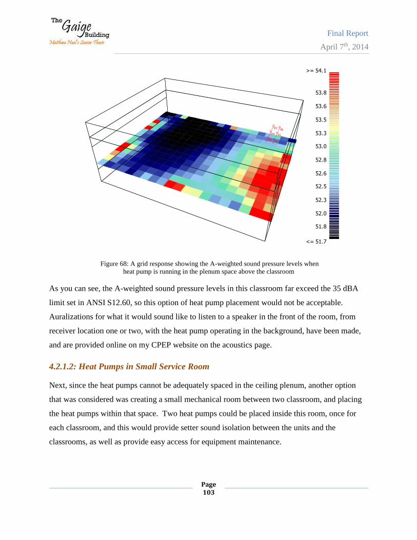
Final Report

April 7th, 2014

Page 103

Figure 68: A grid response showing the A-weighted sound pressure levels when

heat pump is running in the plenum space above the classroom

As you can see, the A-weighted sound pressure levels in this classroom far exceed the 35 dBA

limit set in ANSI S12.60, so this option of heat pump placement would not be acceptable.

Auralizations for what it would sound like to listen to a speaker in the front of the room, from

receiver location one or two, with the heat pump operating in the background, have been made,

and are provided online on my CPEP website on the acoustics page.

4.2.1.2: Heat Pumps in Small Service Room

Next, since the heat pumps cannot be adequately spaced in the ceiling plenum, another option

that was considered was creating a small mechanical room between two classroom, and placing

the heat pumps within that space. Two heat pumps could be placed inside this room, once for

each classroom, and this would provide setter sound isolation between the units and the

classrooms, as well as provide easy access for equipment maintenance.

P2P3P4P5

P6P7

53.8

53.6

53.5

53.3

53.0

52.8

52.6

52.5

52.3

52.0

51.8

SPL(A) (dB) >= 54.1

<= 51.7Odeon©1985-2013 Licensed to: Penn State University, USA Restricted version - research and teaching only!

P2P3

P4 P5

P6P7

54.0

54.0

53.8

53.8

53.6

53.5

53.5

53.3

53.3

53.1

53.0

53.0

52.8

52.8

52.6

52.5

52.5

52.3

52.3

52.1

52.0

52.0

51.8

51.8

SPL(A) (dB) >= 54.1


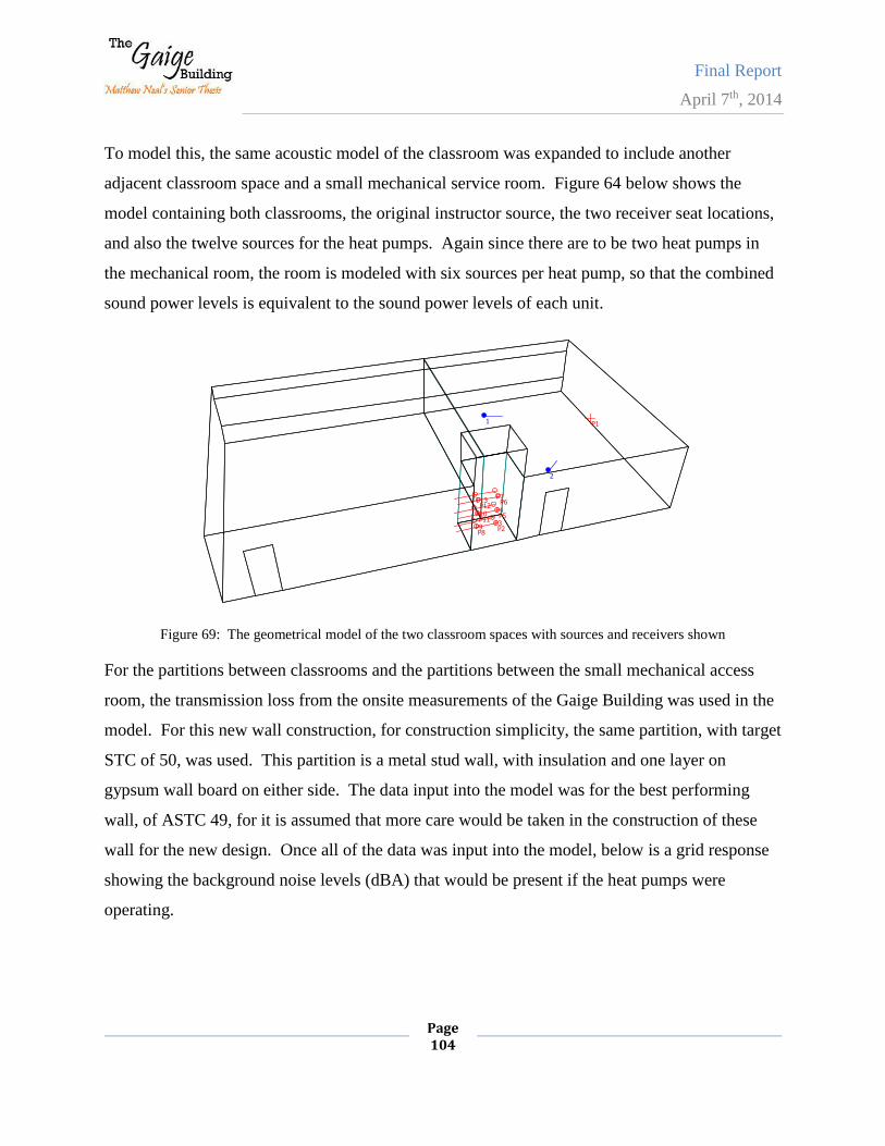
Final Report

April 7th, 2014

Page 104

To model this, the same acoustic model of the classroom was expanded to include another

adjacent classroom space and a small mechanical service room. Figure 64 below shows the

model containing both classrooms, the original instructor source, the two receiver seat locations,

and also the twelve sources for the heat pumps. Again since there are to be two heat pumps in

the mechanical room, the room is modeled with six sources per heat pump, so that the combined

sound power levels is equivalent to the sound power levels of each unit.

Figure 69: The geometrical model of the two classroom spaces with sources and receivers shown

For the partitions between classrooms and the partitions between the small mechanical access

room, the transmission loss from the onsite measurements of the Gaige Building was used in the

model. For this new wall construction, for construction simplicity, the same partition, with target

STC of 50, was used. This partition is a metal stud wall, with insulation and one layer on

gypsum wall board on either side. The data input into the model was for the best performing

wall, of ASTC 49, for it is assumed that more care would be taken in the construction of these

wall for the new design. Once all of the data was input into the model, below is a grid response

showing the background noise levels (dBA) that would be present if the heat pumps were

operating.

OXY

Z

P2P3

P4P5

P6P7

P8P9

P10P11

P12P13

1

2

P1

Odeon©1985-2013 Licensed to: Penn State University, USA Restricted version - research and teaching only!

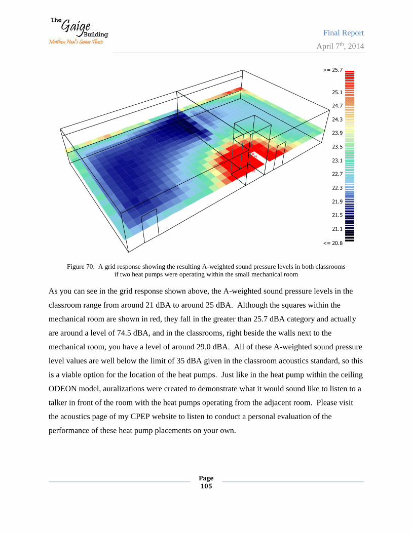
Final Report

April 7th, 2014

Page 105

Figure 70: A grid response showing the resulting A-weighted sound pressure levels in both classrooms

if two heat pumps were operating within the small mechanical room

As you can see in the grid response shown above, the A-weighted sound pressure levels in the

classroom range from around 21 dBA to around 25 dBA. Although the squares within the

mechanical room are shown in red, they fall in the greater than 25.7 dBA category and actually

are around a level of 74.5 dBA, and in the classrooms, right beside the walls next to the

mechanical room, you have a level of around 29.0 dBA. All of these A-weighted sound pressure

level values are well below the limit of 35 dBA given in the classroom acoustics standard, so this

is a viable option for the location of the heat pumps. Just like in the heat pump within the ceiling

ODEON model, auralizations were created to demonstrate what it would sound like to listen to a

talker in front of the room with the heat pumps operating from the adjacent room. Please visit

the acoustics page of my CPEP website to listen to conduct a personal evaluation of the

performance of these heat pump placements on your own.

P2P3

P4P5

P6P7

P8P9

P10P11

P12P13

25.5

25.3

25.1

24.9

24.7

24.5

24.3

24.1

23.9

23.7

23.5

23.3

23.1

22.9

22.7

22.5

22.3

22.1

21.9

21.7

21.5

21.3

21.1

20.9

SPL(A) (dB) >= 25.7


P2P3

P4P5

P6P7

P8P9

P10P11

P12P13

25.1

24.7

24.3

23.9

23.5

23.1

22.7

22.3

21.9

21.5

21.1

SPL(A) (dB) >= 25.7


Final Report

April 7th, 2014

Page 106

4.2.2: Analysis of Sound Isolation through Partitions

Overall, with the addition of the heat pumps within the Gaige Building, it is suggested that for

large spaces, such as classrooms or laboratory spaces, small mechanical access rooms be added

throughout the architectural design. This would allow for easy maintenance access to the water

source heat pumps, and as shown in the previous analysis. The heat pumps are too loud to place

in the plenum space above the ceiling, so this is a good option.

For smaller spaces, such as the offices, it is recommended that the walls between the corridors

and the offices be built to structure, and the heat pumps places above the plenum space in the

hallway. This would allow the noise sources to be located in a less noise sensitive space, such as

the hallway. The designer should now specify similar performing wall between the corridors and

the offices, otherwise, the performance modeled with the heat pump in the small room adjacent

to the classroom will not be reached. A poor performing partition will not adequately isolate the

heat pumps in the corridor plenum space from the office space. Currently, the walls between the

hallway and the offices are not built to structure, so this would need to be specified in the new

design.

4.2.3: Analysis of Air Noise through Diffusers

Finally, the other source of noise from the heat pumps would be noise traveling through the

ductwork into the space. To ensure that this airside noise would not be an issue, a duct noise

modeling program was used to model the ductwork extending from the heat pumps for a

classroom and a private office space, since these are the most noise sensitive. The sound power

levels of noise from the ducted supply was input into Dynasonics, and a return path and supply

path were added to both the classroom and the office.

To the classroom, the path was modeled with a return path containing two elbows, one takeoff,

15 feet of rectangular duct, flex duct that connected into the supply diffuser, end reflection loss,

and a room correction factor. For the supply path, the ductwork was modeled with one elbow,

one takeoff, 11 feet of rectangular ductwork, flex duct connection to the diffuser, end reflection

loss, and a room correction factor. After combining these two path effects into the room

together, the NC levels for the room were too high, but only in the upper frequency ranges. To

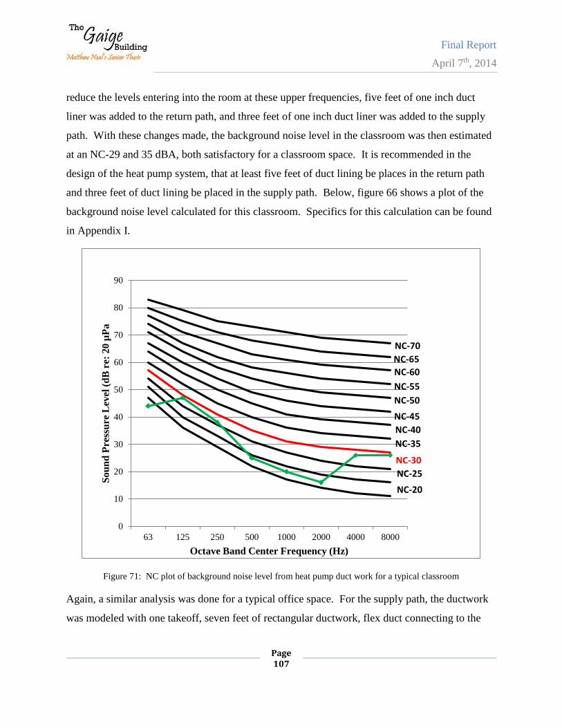
Final Report

April 7th, 2014

Page 107

reduce the levels entering into the room at these upper frequencies, five feet of one inch duct

liner was added to the return path, and three feet of one inch duct liner was added to the supply

path. With these changes made, the background noise level in the classroom was then estimated

at an NC-29 and 35 dBA, both satisfactory for a classroom space. It is recommended in the

design of the heat pump system, that at least five feet of duct lining be places in the return path

and three feet of duct lining be placed in the supply path. Below, figure 66 shows a plot of the

background noise level calculated for this classroom. Specifics for this calculation can be found

in Appendix I.

Figure 71: NC plot of background noise level from heat pump duct work for a typical classroom

Again, a similar analysis was done for a typical office space. For the supply path, the ductwork

was modeled with one takeoff, seven feet of rectangular ductwork, flex duct connecting to the

0

10

20

30

40

50

60

70

80

90

63 125 250 500 1000 2000 4000 8000

Sou

nd

Pre

ssu

re L

evel

(d

B r

e: 2

0 µ

Pa


NC-20

NC-25

NC-30

NC-35

NC-40

NC-45

NC-50

NC-55

NC-60

NC-65

NC-70

Final Report

April 7th, 2014

Page 108

diffuser, end reflection loss, and a room correction factor. Also, the return path was modeled

with one takeoff, seven feet of rectangular ductwork, flex duct connecting to the diffuser, end

reflection loss, and also a room corrections factor. With both of these paths added together, there

was again some noise control issues in the higher frequencies, so three feet of one inch duct liner

was added to the supply path and two feet of one inch duct liner was added to the supply path.

With this addition, the office was then calculated to be at NC-27 at a level of 34 dBA. This met

the requirements for a private office of NC-30, so the design was considered successful. For the

office spaces in the Gaige Building, for offices close to the heat pumps, at least three feet of duct

lining should be placed in the supply path, and at least two feet of duct lining should be placed in

the return path. Below, in figure 67, you can see an NC plot containing the background noise

levels for this typical office.

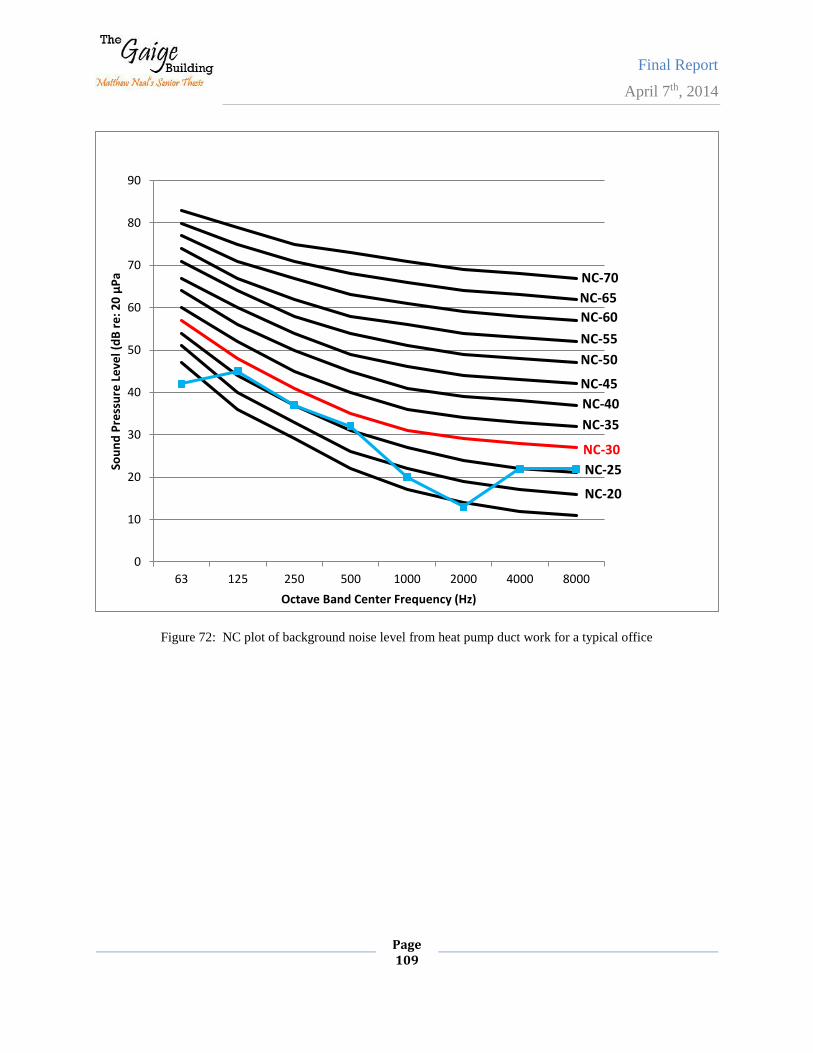
Final Report

April 7th, 2014

Page 109

Figure 72: NC plot of background noise level from heat pump duct work for a typical office

0

10

20

30

40

50

60

70

80

90

63 125 250 500 1000 2000 4000 8000

Sou

nd

Pre

ssu

re L

eve

l (d

B r

e: 2

0 µ

Pa


NC-20

NC-25

NC-30

NC-35

NC-40

NC-45

NC-50

NC-55

NC-60

NC-65

NC-70

Final Report

April 7th, 2014

Page 110

Chapter 5: Construction Breadth

When considering whether or not a geothermal system will be a favorable option for your

building, the most important, and normally the make or break decision is centered around cost.

The justification behind a geothermal system is that the increased initial costs of the building will

be justified, and ultimately paid off from the annual energy savings in the long run. You want to

be able to show that a system will pay itself off within a reasonable amount of time, typically

within the lifetime of a system. To do so, information on what increased costs will result from

the addition of various system parts must be determined, estimated, and included in any life

cycle cost analysis. For the construction breadth of this thesis, costs estimations are made for the

Gaige Building, estimating the increase in initial costs due to the addition of water source heat

pump, outdoor air units, piping, and large costs associated with the installation of a horizontal

well field. RS Means Building and Mechanical cost reference data was used for this analysis.

Below each section summarized the main considerations made in this design, and presents the

overall cost analysis results. The results of these estimations were used the analyses in section

3.1, for the life cycle cost analysis of the Gaige Building geothermal system. These values were

used to help determine the initial increase in first costs.

4.1: Geothermal Bore Cost Evaluation

The major costs associated with any geothermal installation is in the materials, labor, and

equipment used in the installation of the geothermal well field. For the Gaige Building, two

different types of well field arrangements are being considered: a horizontal loop system and a

vertical loops system. Both system have their pros and cons, but the main considerations are

space and costs. The vertical loop system takes up much less space than the horizontal loop

system, but it typically costs more to install and construct on a per length of well basis. In the

next two sections, 4.1.1 and 4.1.2, costs are estimated for the construction of a vertical and a

horizontal geothermal loop system. Then, to help determine which loop is a better cost, they are

compared, both using a constant length of cooling.

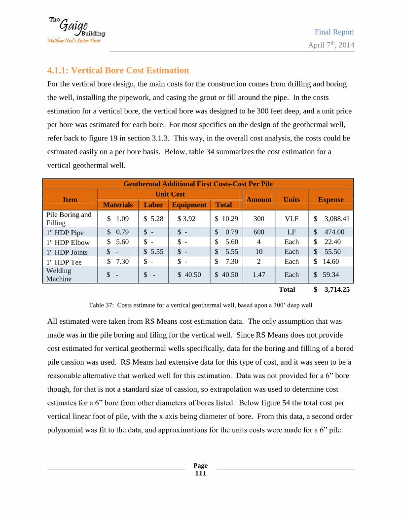
Final Report

April 7th, 2014

Page 111

4.1.1: Vertical Bore Cost Estimation

For the vertical bore design, the main costs for the construction comes from drilling and boring

the well, installing the pipework, and casing the grout or fill around the pipe. In the costs

estimation for a vertical bore, the vertical bore was designed to be 300 feet deep, and a unit price

per bore was estimated for each bore. For most specifics on the design of the geothermal well,

refer back to figure 19 in section 3.1.3. This way, in the overall cost analysis, the costs could be

estimated easily on a per bore basis. Below, table 34 summarizes the cost estimation for a

vertical geothermal well.

Geothermal Additional First Costs-Cost Per Pile

Item Unit Cost

Amount Units Expense Materials Labor Equipment Total

Pile Boring and

Filling $ 1.09 $ 5.28 $ 3.92 $ 10.29 300 VLF $ 3,088.41

1" HDP Pipe $ 0.79 $ - $ - $ 0.79 600 LF $ 474.00

1" HDP Elbow $ 5.60 $ - $ - $ 5.60 4 Each $ 22.40

1" HDP Joints $ - $ 5.55 $ - $ 5.55 10 Each $ 55.50

1" HDP Tee $ 7.30 $ - $ - $ 7.30 2 Each $ 14.60

Welding

Machine $ - $ - $ 40.50 $ 40.50 1.47 Each $ 59.34

Total $ 3,714.25

Table 37: Costs estimate for a vertical geothermal well, based upon a 300’ deep well

All estimated were taken from RS Means cost estimation data. The only assumption that was

made was in the pile boring and filing for the vertical well. Since RS Means does not provide

cost estimated for vertical geothermal wells specifically, data for the boring and filling of a bored

pile cassion was used. RS Means had extensive data for this type of cost, and it was seen to be a

reasonable alternative that worked well for this estimation. Data was not provided for a 6” bore

though, for that is not a standard size of cassion, so extrapolation was used to determine cost

estimates for a 6” bore from other diameters of bores listed. Below figure 54 the total cost per

vertical linear foot of pile, with the x axis being diameter of bore. From this data, a second order

polynomial was fit to the data, and approximations for the units costs were made for a 6” pile.

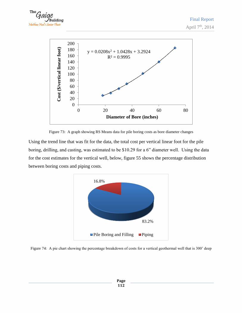
Final Report

April 7th, 2014

Page 112

Figure 73: A graph showing RS Means data for pile boring costs as bore diameter changes

Using the trend line that was fit for the data, the total cost per vertical linear foot for the pile

boring, drilling, and casting, was estimated to be $10.29 for a 6” diameter well. Using the data

for the cost estimates for the vertical well, below, figure 55 shows the percentage distribution

between boring costs and piping costs.

Figure 74: A pie chart showing the percentage breakdown of costs for a vertical geothermal well that is 300’ deep

y = 0.0208x2 + 1.0428x + 3.2924

R² = 0.9995

0

20

40

60

80

100

120

140

160

180

200

0 20 40 60 80

Cost

($/v

erti

cal

lin

ear

foot)

Diameter of Bore (inches)

83.2%

16.8%

Pile Boring and Filling Piping

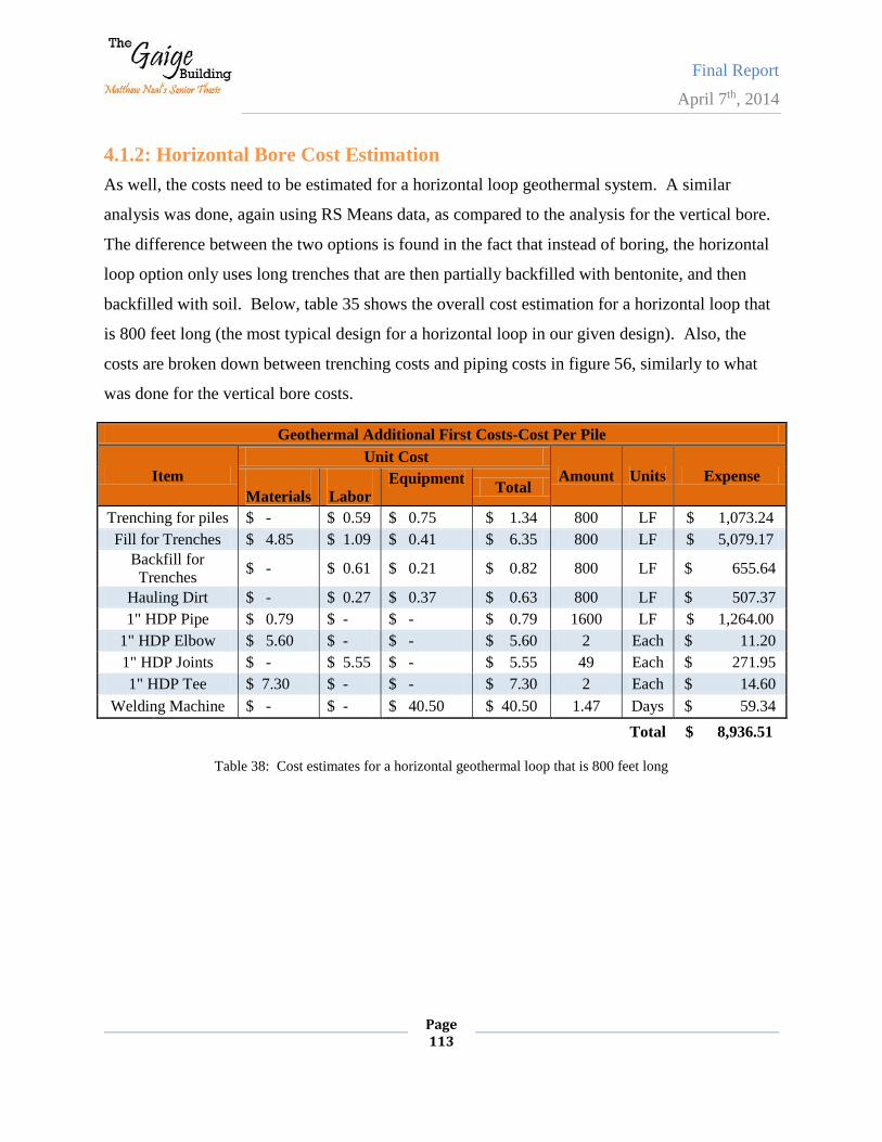
Final Report

April 7th, 2014

Page 113

4.1.2: Horizontal Bore Cost Estimation

As well, the costs need to be estimated for a horizontal loop geothermal system. A similar

analysis was done, again using RS Means data, as compared to the analysis for the vertical bore.

The difference between the two options is found in the fact that instead of boring, the horizontal

loop option only uses long trenches that are then partially backfilled with bentonite, and then

backfilled with soil. Below, table 35 shows the overall cost estimation for a horizontal loop that

is 800 feet long (the most typical design for a horizontal loop in our given design). Also, the

costs are broken down between trenching costs and piping costs in figure 56, similarly to what

was done for the vertical bore costs.

Geothermal Additional First Costs-Cost Per Pile

Item

Unit Cost

Amount Units Expense

Materials

Labor

Equipment Total

Trenching for piles $ - $ 0.59 $ 0.75 $ 1.34 800 LF $ 1,073.24

Fill for Trenches $ 4.85 $ 1.09 $ 0.41 $ 6.35 800 LF $ 5,079.17

Backfill for

Trenches $ - $ 0.61 $ 0.21 $ 0.82 800 LF $ 655.64

Hauling Dirt $ - $ 0.27 $ 0.37 $ 0.63 800 LF $ 507.37

1" HDP Pipe $ 0.79 $ - $ - $ 0.79 1600 LF $ 1,264.00

1" HDP Elbow $ 5.60 $ - $ - $ 5.60 2 Each $ 11.20

1" HDP Joints $ - $ 5.55 $ - $ 5.55 49 Each $ 271.95

1" HDP Tee $ 7.30 $ - $ - $ 7.30 2 Each $ 14.60

Welding Machine $ - $ - $ 40.50 $ 40.50 1.47 Days $ 59.34

Total $ 8,936.51

Table 38: Cost estimates for a horizontal geothermal loop that is 800 feet long

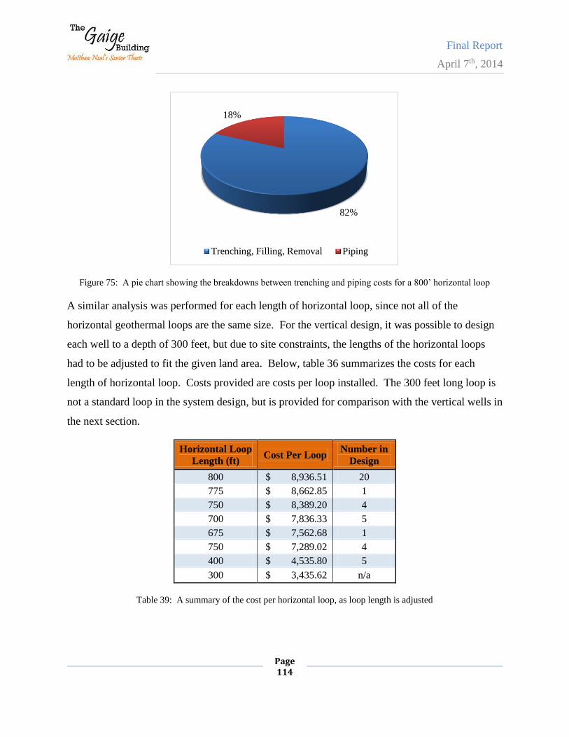
Final Report

April 7th, 2014

Page 114

Figure 75: A pie chart showing the breakdowns between trenching and piping costs for a 800’ horizontal loop

A similar analysis was performed for each length of horizontal loop, since not all of the

horizontal geothermal loops are the same size. For the vertical design, it was possible to design

each well to a depth of 300 feet, but due to site constraints, the lengths of the horizontal loops

had to be adjusted to fit the given land area. Below, table 36 summarizes the costs for each

length of horizontal loop. Costs provided are costs per loop installed. The 300 feet long loop is

not a standard loop in the system design, but is provided for comparison with the vertical wells in

the next section.

Horizontal Loop

Length (ft) Cost Per Loop

Number in

Design

800 $ 8,936.51 20

775 $ 8,662.85 1

750 $ 8,389.20 4

700 $ 7,836.33 5

675 $ 7,562.68 1

750 $ 7,289.02 4

400 $ 4,535.80 5

300 $ 3,435.62 n/a

Table 39: A summary of the cost per horizontal loop, as loop length is adjusted

82%

18%

Trenching, Filling, Removal Piping

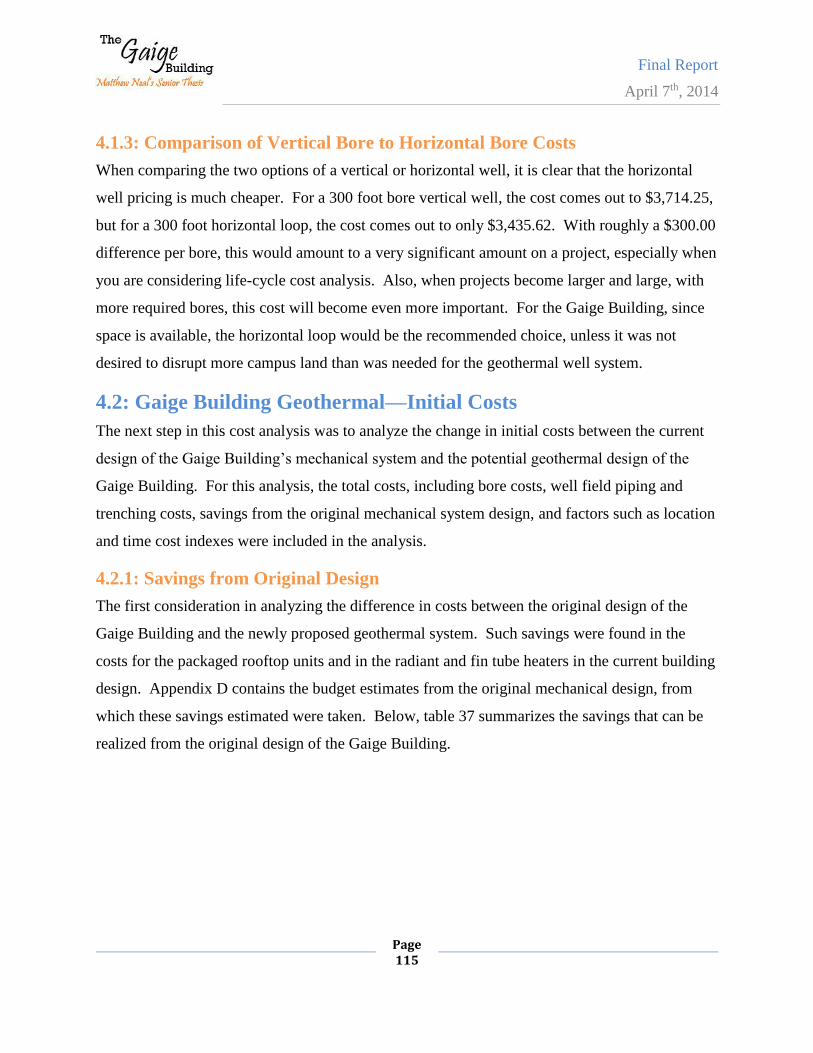
Final Report

April 7th, 2014

Page 115

4.1.3: Comparison of Vertical Bore to Horizontal Bore Costs

When comparing the two options of a vertical or horizontal well, it is clear that the horizontal

well pricing is much cheaper. For a 300 foot bore vertical well, the cost comes out to $3,714.25,

but for a 300 foot horizontal loop, the cost comes out to only $3,435.62. With roughly a $300.00

difference per bore, this would amount to a very significant amount on a project, especially when

you are considering life-cycle cost analysis. Also, when projects become larger and large, with

more required bores, this cost will become even more important. For the Gaige Building, since

space is available, the horizontal loop would be the recommended choice, unless it was not

desired to disrupt more campus land than was needed for the geothermal well system.

4.2: Gaige Building Geothermal—Initial Costs

The next step in this cost analysis was to analyze the change in initial costs between the current

design of the Gaige Building’s mechanical system and the potential geothermal design of the

Gaige Building. For this analysis, the total costs, including bore costs, well field piping and

trenching costs, savings from the original mechanical system design, and factors such as location

and time cost indexes were included in the analysis.

4.2.1: Savings from Original Design

The first consideration in analyzing the difference in costs between the original design of the

Gaige Building and the newly proposed geothermal system. Such savings were found in the

costs for the packaged rooftop units and in the radiant and fin tube heaters in the current building

design. Appendix D contains the budget estimates from the original mechanical design, from

which these savings estimated were taken. Below, table 37 summarizes the savings that can be

realized from the original design of the Gaige Building.

Final Report

April 7th, 2014

Page 116

Geothermal Cost Savings

Item Unit Cost Amount Units Savings

RTU's - Quote (20,500, 14,000, 10,725 CFM's) $ 300,000.00 1 All $ 300,000.00

RTU Installation $ 2.00 45,230 CFM $ 90,460.00

Fin Tubes $ 75.00 1150 LF $ 86,250.00

Radiant Heat Panels $ 100.00 80 Each $ 8,000.00

$ 484,710.00

Table 40: Summary of cost savings that can be realized from the original Gaige Building’s design

4.2.2: Initial Costs for Vertical Bore Design

For the vertical well field, costs were estimated to determine the increase in initial costs due to

the addition of the new equipment, piping, and labor that would need to be done to estimate the

costs for the new Gaige Building geothermal design. In this cost analysis, considerations for

heat pumps costs in the building, heat pump piping costs, building centrifugal pumps, geothermal

pumps, geothermal piping, well field costs, and DOAS costs were all considered in the analysis.

For the details of the specific analysis for the proposed vertical well field design, see Appendix

F. Overall, the total increase in cost due to the building and well field construction costs came

out to be $655,736.06. Now, to determine the overall additional first costs for the life-cycle cost

analysis, the savings must be incorporated into this analysis. First, the savings estimate is

adjusted from its estimation year of 2009 to the present year of 2014. Then, the cost estimate for

the building and well field increased costs are adjusted using a location multiplier of 0.988,

which is the overall location based multiplier for Reading, PA as provided by RS Means data.

Table 38 below summarizes this analysis, and presents a total increase in initial first costs for the

vertical geothermal well field of $102,636.63

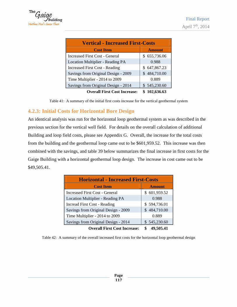
Final Report

April 7th, 2014

Page 117

Vertical - Increased First-Costs

Cost Item Amount



Increased First Cost - Reading $ 647,867.23





Table 41: A summary of the initial first costs increase for the vertical geothermal system

4.2.3: Initial Costs for Horizontal Bore Design

An identical analysis was run for the horizontal loop geothermal system as was described in the

previous section for the vertical well field. For details on the overall calculation of additional

Building and loop field costs, please see Appendix G. Overall, the increase for the total costs

from the building and the geothermal loop came out to be $601,959.52. This increase was then

combined with the savings, and table 39 below summarizes the final increase in first costs for the

Gaige Building with a horizontal geothermal loop design. The increase in cost came out to be

$49,505.41.


Cost Item Amount








Table 42: A summary of the overall increased first costs for the horizontal loop geothermal design

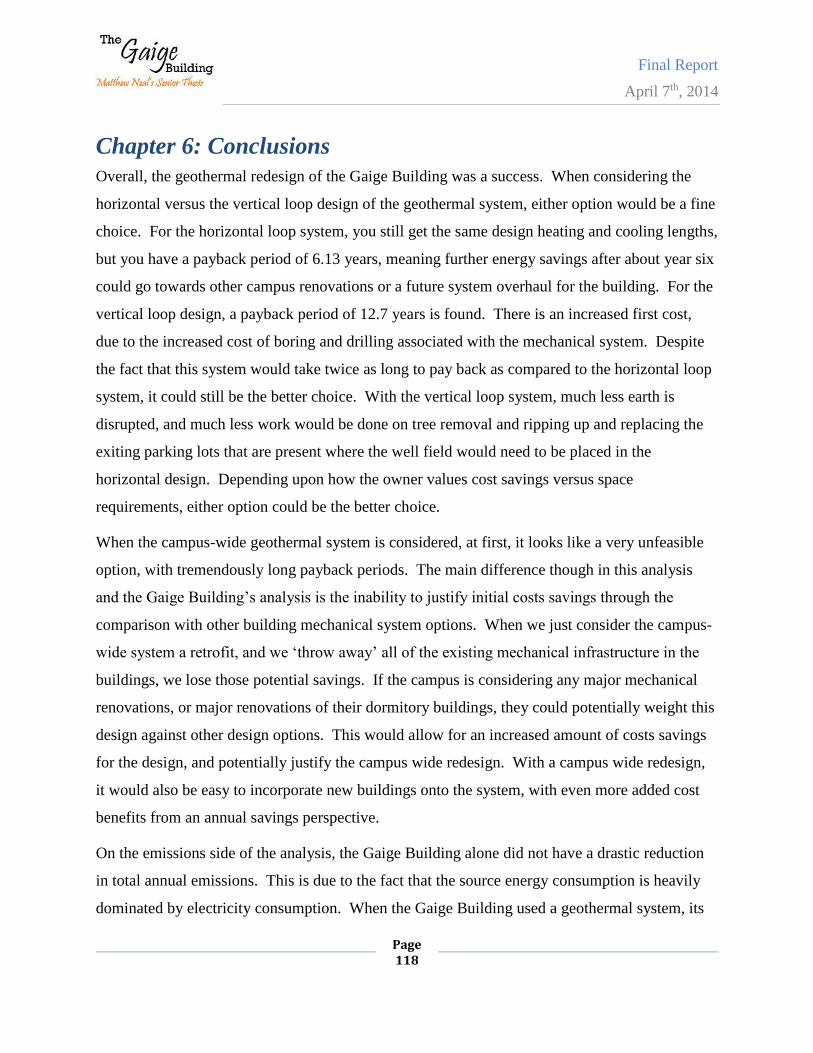
Final Report

April 7th, 2014

Page 118

Chapter 6: Conclusions

Overall, the geothermal redesign of the Gaige Building was a success. When considering the

horizontal versus the vertical loop design of the geothermal system, either option would be a fine

choice. For the horizontal loop system, you still get the same design heating and cooling lengths,

but you have a payback period of 6.13 years, meaning further energy savings after about year six

could go towards other campus renovations or a future system overhaul for the building. For the

vertical loop design, a payback period of 12.7 years is found. There is an increased first cost,

due to the increased cost of boring and drilling associated with the mechanical system. Despite

the fact that this system would take twice as long to pay back as compared to the horizontal loop

system, it could still be the better choice. With the vertical loop system, much less earth is

disrupted, and much less work would be done on tree removal and ripping up and replacing the

exiting parking lots that are present where the well field would need to be placed in the

horizontal design. Depending upon how the owner values cost savings versus space

requirements, either option could be the better choice.

When the campus-wide geothermal system is considered, at first, it looks like a very unfeasible

option, with tremendously long payback periods. The main difference though in this analysis

and the Gaige Building’s analysis is the inability to justify initial costs savings through the

comparison with other building mechanical system options. When we just consider the campus-

wide system a retrofit, and we ‘throw away’ all of the existing mechanical infrastructure in the

buildings, we lose those potential savings. If the campus is considering any major mechanical

renovations, or major renovations of their dormitory buildings, they could potentially weight this

design against other design options. This would allow for an increased amount of costs savings

for the design, and potentially justify the campus wide redesign. With a campus wide redesign,

it would also be easy to incorporate new buildings onto the system, with even more added cost

benefits from an annual savings perspective.

On the emissions side of the analysis, the Gaige Building alone did not have a drastic reduction

in total annual emissions. This is due to the fact that the source energy consumption is heavily

dominated by electricity consumption. When the Gaige Building used a geothermal system, its

Final Report

April 7th, 2014

Page 119

savings were really found by reducing the natural gas loads. The cooling load electrical savings

were covered up by the increase in electricity consumption due to the operation of many

different heat pumps throughout the building. On the other hand, when a campus wide

geothermal system was considered, it had a 27% reduction in annual emissions, a drastic impact

upon the campus total emissions. This was mainly influenced by the building that ran solely off

of electricity as their cooling and heating source. Since electricity has a large impact upon

source energy consumption, and the fact that all of the savings from these types of buildings was

on the electrical bill, it had a large impact upon annual emissions. With these savings realized,

this is another arguments that is strong in the favor of a high capacity, campus-wide geothermal

system, ignoring the life-cycle cost feasibility questions.

Finally, a thorough acoustic analysis of the Gaige Building was conducted. As compared to

ANSI S12.60, the classroom acoustics standard, the Gaige Building did a great job. All six of

the measured classroom exhibited adequate reverberation times, and adequate background noise

levels. There were some low frequency reverberation issues, but this is understandable due to

the low frequency absorption limitation of porous type absorbers. Two out of four of the tested

partitions performed will, with an ASTC measuring at least 46 for a specified design STC of 50.

On the other hand, both of the partitions tested on the second floor did not perform well, having

ASTC ratings of 38 and 40, for a wall with a design STC of 50. The severe underperformance

was due to poor sealing of the place where the partition met continuous window glazing. This

poor sealing left visible gaps between the wall and window construction, short-circuiting the

sound transmission performance of the wall, and thus, drastically decreasing the STC of the wall.

Finally, it was found that the best placement for the geothermal water source heat pumps would

be in the hallway ceiling plenum for the offices, now with the wall between the hallway and the

offices built to structure. Also, to properly isolate the heat pumps from the classroom spaces,

additional mechanical access rooms should be placed near existing classrooms and labs. This

allows for proper sound isolation, with easy access to the heat pumps for maintenance purposes.

Finally, guidelines for controlling duct noise from the heat pumps was provided to ensure

adequate NC-levels in the offices and classroom are met.

Final Report

April 7th, 2014

Page 120

References

ANSI/ASHRAE. (2010). Standard 62.1-2007, Ventilation for Acceptable Indoor Air Quality.

Atlanta, GA: American Society of Heating Refrigeration and Air Conditioning Engineers, Inc.

ANSI/ASHRAE. (2010). Standard 90.1-2007, Energy Standard for Buildings Except Low-Rise

Residential Buildings. Atlanta, GA: American Society of Heating Refrigeration and Air

Conditioning Engineers, Inc.

ASHRAE. (2009). Handbook of Fundamentals. Atlanta, GA: American Society of Heating

Refrigeration and Air Conditioning Engineers, Inc.

ASHRAE. (2011). Applications, Chapter 34, Geothermal Energy. Atlanta, GA: American

Society of Heating Refrigeration and Air Conditioning Engineers, Inc.

EIA. (2012). Pennsylvania Energy Fact Sheet. Washington, DC: United States Energy

Information Administration

Deru, M. and Torcellini, P. (2007). Technical Report NREL/TP-550-38617, Source Energy and

Emission Factors for Energy Use in Buildings. Golden, CO: Nation Renewable Energy

Laboratory

H. F. Lenz Company, LLP. Electrical, Mechanical, and Plumbing Construction Documents. H.

F. Lenz Company, Johnstown, PA

H. F. Lenz Company, LLP. Electrical, Mechanical, and Plumbing Construction Specifications.

H. F. Lenz Company, Johnstown, PA

RMJM Hillier Architects. Architectural Construction Documents. RMJM/Hillier Architecture,

New York,

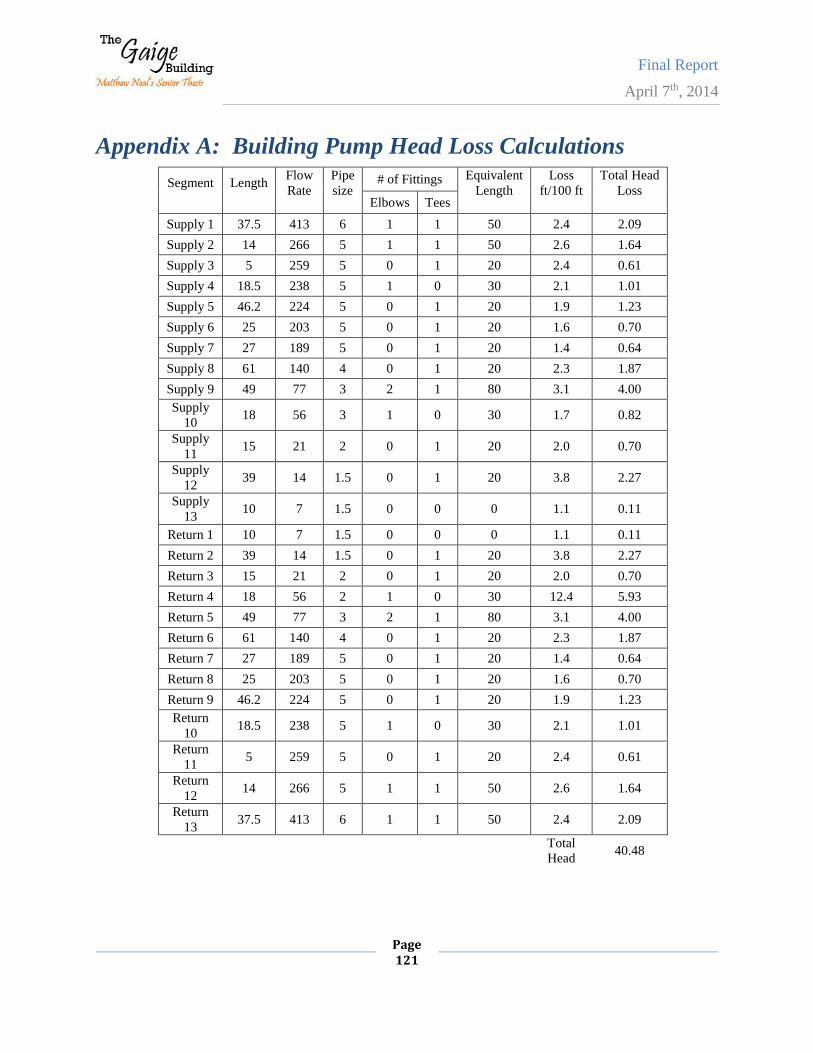
Final Report

April 7th, 2014

Page 121

Appendix A: Building Pump Head Loss Calculations

Segment

Length

Flow

Rate

Pipe

size


Length

Loss

ft/100 ft

Total Head

Loss

Elbows Tees

Supply 1 37.5 413 6 1 1 50 2.4 2.09

Supply 2 14 266 5 1 1 50 2.6 1.64

Supply 3 5 259 5 0 1 20 2.4 0.61

Supply 4 18.5 238 5 1 0 30 2.1 1.01

Supply 5 46.2 224 5 0 1 20 1.9 1.23

Supply 6 25 203 5 0 1 20 1.6 0.70

Supply 7 27 189 5 0 1 20 1.4 0.64

Supply 8 61 140 4 0 1 20 2.3 1.87

Supply 9 49 77 3 2 1 80 3.1 4.00

Supply

10 18 56 3 1 0 30 1.7 0.82

Supply

11 15 21 2 0 1 20 2.0 0.70

Supply

12 39 14 1.5 0 1 20 3.8 2.27

Supply

13 10 7 1.5 0 0 0 1.1 0.11

Return 1 10 7 1.5 0 0 0 1.1 0.11

Return 2 39 14 1.5 0 1 20 3.8 2.27

Return 3 15 21 2 0 1 20 2.0 0.70

Return 4 18 56 2 1 0 30 12.4 5.93

Return 5 49 77 3 2 1 80 3.1 4.00

Return 6 61 140 4 0 1 20 2.3 1.87

Return 7 27 189 5 0 1 20 1.4 0.64

Return 8 25 203 5 0 1 20 1.6 0.70

Return 9 46.2 224 5 0 1 20 1.9 1.23

Return

10 18.5 238 5 1 0 30 2.1 1.01

Return

11 5 259 5 0 1 20 2.4 0.61

Return

12 14 266 5 1 1 50 2.6 1.64

Return

13 37.5 413 6 1 1 50 2.4 2.09

Total

Head 40.48

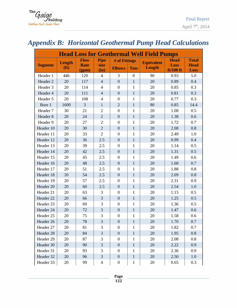
Final Report

April 7th, 2014

Page 122

Appendix B: Horizontal Geothermal Pump Head Calculations

Head Loss for Geothermal Well Field Pumps

Segment Length

(ft)

Flow

Rate

(gpm)

Pipe

size

(in)


Length

Head

Loss

ft/100 ft

Total

Head

Loss Elbows Tees

Header 1 446 120 4 3 0 90 0.93 5.0

Header 2 20 117 4 0 1 20 0.89 0.4

Header 3 20 114 4 0 1 20 0.85 0.3

Header 4 20 111 4 0 1 20 0.81 0.3

Header 5 20 108 4 0 1 20 0.77 0.3

Bore 1 1600 3 1 2 1 80 0.85 14.4

Header 7 30 21 2 0 1 20 1.08 0.5

Header 8 20 24 2 0 1 20 1.38 0.6

Header 9 20 27 2 0 1 20 1.72 0.7

Header 10 20 30 2 0 1 20 2.08 0.8

Header 11 20 33 2 0 1 20 2.49 1.0

Header 12 20 36 2.5 0 1 20 0.99 0.4

Header 13 20 39 2.5 0 1 20 1.14 0.5

Header 14 20 42 2.5 0 1 20 1.31 0.5

Header 15 20 45 2.5 0 1 20 1.49 0.6

Header 16 20 48 2.5 0 1 20 1.68 0.7

Header 17 20 51 2.5 0 1 20 1.88 0.8

Header 18 20 54 2.5 0 1 20 2.09 0.8

Header 19 20 57 2.5 0 1 20 2.31 0.9

Header 20 20 60 2.5 0 1 20 2.54 1.0

Header 21 20 63 3 0 1 20 1.15 0.5

Header 22 20 66 3 0 1 20 1.25 0.5

Header 23 20 69 3 0 1 20 1.36 0.5

Header 24 20 72 3 0 1 20 1.47 0.6

Header 25 20 75 3 0 1 20 1.58 0.6

Header 26 20 78 3 0 1 20 1.70 0.7

Header 27 20 81 3 0 1 20 1.82 0.7

Header 28 20 84 3 0 1 20 1.95 0.8

Header 29 20 87 3 0 1 20 2.08 0.8

Header 30 20 90 3 0 1 20 2.22 0.9

Header 31 20 93 3 0 1 20 2.36 0.9

Header 32 20 96 3 0 1 20 2.50 1.0

Header 33 20 99 4 0 1 20 0.65 0.3

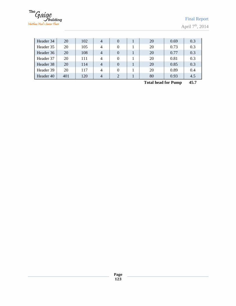
Final Report

April 7th, 2014

Page 123

Header 34 20 102 4 0 1 20 0.69 0.3

Header 35 20 105 4 0 1 20 0.73 0.3

Header 36 20 108 4 0 1 20 0.77 0.3

Header 37 20 111 4 0 1 20 0.81 0.3

Header 38 20 114 4 0 1 20 0.85 0.3

Header 39 20 117 4 0 1 20 0.89 0.4

Header 40 401 120 4 2 1 80 0.93 4.5

Total head for Pump 45.7

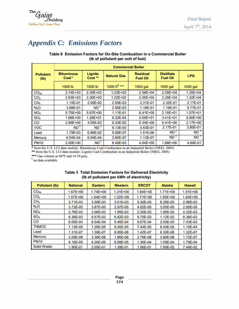
Final Report

April 7th, 2014

Page 124

Appendix C: Emissions Factors

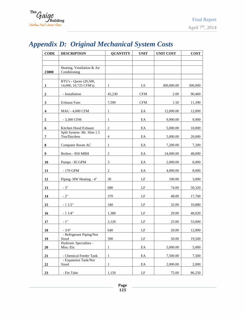
Final Report

April 7th, 2014

Page 125

Appendix D: Original Mechanical System Costs

CODE DESCRIPTION QUANTITY UNIT UNIT COST COST

23000

Heating, Ventilation & Air

Conditioning

1

RTU's - Quote (20,500,

14,000, 10,725 CFM's)

1 LS 300,000.00 300,000

2 - Installation

45,230 CFM 2.00 90,460

3 Exhaust Fans

7,590 CFM 1.50 11,390

4 MAU - 4,000 CFM

1 EA 12,000.00 12,000

5 - 3,300 CFM

1 EA 9,900.00 9,900

6 Kitchen Hood Exhaust

2 EA 5,000.00 10,000

7

Split System- Mr. Slim 1.5

Ton/Ductless

4 EA 5,000.00 20,000

8 Computer Room AC

1 EA 7,200.00 7,200

9 Boilers - 850 MBH

2 EA 24,000.00 48,000

10 Pumps - 85 GPM

3 EA 2,000.00 6,000

11 - 170 GPM

2 EA 4,000.00 8,000

12 Piping- HW Heating - 4"

30 LF 100.00 3,000

13 - 3"

680 LF 74.00 50,320

14 - 2"

370 LF 48.00 17,760

15 - 1 1/2"

340 LF 32.00 10,880

16 - 1 1/4"

1,380 LF 29.00 40,020

17 - 1"

2,120 LF 25.00 53,000

18 - 3/4"

640 LF 20.00 12,800

19

- Refrigerant Piping/Not

Sized

390 LF 50.00 19,500

20

Hydronic Specialties -

Misc./Etc

1 EA 5,000.00 5,000

21 - Chemical Feeder Tank

1 EA 7,500.00 7,500

22

- Expansion Tank/Not

Sized

1 EA 2,000.00 2,000

23 - Fin Tube

1,150 LF 75.00 86,250

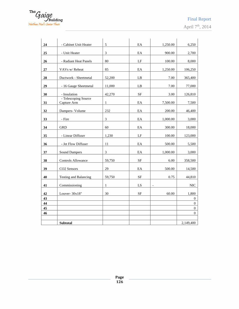
Final Report

April 7th, 2014

Page 126

24 - Cabinet Unit Heater

5 EA 1,250.00 6,250

25 - Unit Heater

3 EA 900.00 2,700

26 - Radiant Heat Panels

80 LF 100.00 8,000

27 VAVs w/ Reheat

85 EA 1,250.00 106,250

28 Ductwork - Sheetmetal

52,200 LB 7.00 365,400

29 - 16 Gauge Sheetmetal

11,000 LB 7.00 77,000

30 - Insulation

42,270 SF 3.00 126,810

31

- Telescoping Source

Capture Arm

1 EA 7,500.00 7,500

32 Dampers- Volume

232 EA 200.00 46,400

33 - Fire

3 EA 1,000.00 3,000

34 GRD

60 EA 300.00 18,000

35 - Linear Diffuser

1,230 LF 100.00 123,000

36 - Jet Flow Diffuser

11 EA 500.00 5,500

37 Sound Dampers

3 EA 1,000.00 3,000

38 Controls Allowance

59,750 SF 6.00 358,500

39 CO2 Sensors

29 EA 500.00 14,500

40 Testing and Balancing

59,750 SF 0.75 44,810

41 Commissioning

1 LS - NIC

42 Louver- 30x18"

30 SF 60.00 1,800

43 0

44 0

45 0

46 0

Subtotal 2,149,400

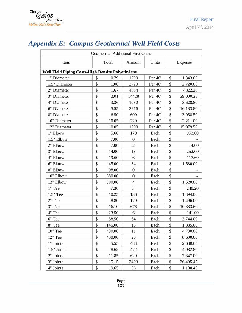
Final Report

April 7th, 2014

Page 127

Appendix E: Campus Geothermal Well Field Costs

Geothermal Additional First Costs

Item Total Amount Units Expense

Well Field Piping Costs-High Density Polyethylene

1" Diameter $ 0.79 1700 Per 40' $ 1,343.00

1.5" Diameter $ 1.00 2720 Per 40' $ 2,720.00

2" Diameter $ 1.67 4684 Per 40' $ 7,822.28

3" Diameter $ 2.01 14428 Per 40' $ 29,000.28

4" Diameter $ 3.36 1080 Per 40' $ 3,628.80

6" Diameter $ 5.55 2916 Per 40' $ 16,183.80

8" Diameter $ 6.50 609 Per 40' $ 3,958.50

10" Diameter $ 10.05 220 Per 40' $ 2,211.00

12" Diameter $ 10.05 1590 Per 40' $ 15,979.50

1" Elbow $ 5.60 170 Each $ 952.00

1.5" Elbow $ 7.00 0 Each $ -

2" Elbow $ 7.00 2 Each $ 14.00

3" Elbow $ 14.00 18 Each $ 252.00

4" Elbow $ 19.60 6 Each $ 117.60

6" Elbow $ 45.00 34 Each $ 1,530.00

8" Elbow $ 98.00 0 Each $ -

10" Elbow $ 380.00 0 Each $ -

12" Elbow $ 380.00 4 Each $ 1,520.00

1" Tee $ 7.30 34 Each $ 248.20

1.5" Tee $ 10.25 136 Each $ 1,394.00

2" Tee $ 8.80 170 Each $ 1,496.00

3" Tee $ 16.10 676 Each $ 10,883.60

4" Tee $ 23.50 6 Each $ 141.00

6" Tee $ 58.50 64 Each $ 3,744.00

8" Tee $ 145.00 13 Each $ 1,885.00

10" Tee $ 430.00 11 Each $ 4,730.00

12" Tee $ 430.00 20 Each $ 8,600.00

1" Joints $ 5.55 483 Each $ 2,680.65

1.5" Joints $ 8.65 472 Each $ 4,082.80

2" Joints $ 11.85 620 Each $ 7,347.00

3" Joints $ 15.15 2403 Each $ 36,405.45

4" Joints $ 19.65 56 Each $ 1,100.40

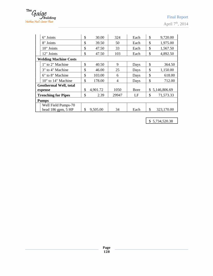
Final Report

April 7th, 2014

Page 128

6" Joints $ 30.00 324 Each $ 9,720.00

8" Joints $ 39.50 50 Each $ 1,975.00

10" Joints $ 47.50 33 Each $ 1,567.50

12" Joints $ 47.50 103 Each $ 4,892.50

Welding Machine Costs

1" to 2" Machine $ 40.50 9 Days $ 364.50

3" to 4" Machine $ 46.00 25 Days $ 1,150.00

6" to 8" Machine $ 103.00 6 Days $ 618.00

10" to 14" Machine $ 178.00 4 Days $ 712.00

Geothermal Well, total

expense $ 4,901.72 1050 Bore $ 5,146,806.69

Trenching for Pipes $ 2.39 29947 LF $ 71,573.33

Pumps

Well Field Pumps-70

head 186 gpm, 5 HP $ 9,505.00 34 Each $ 323,170.00

$ 5,734,520.38

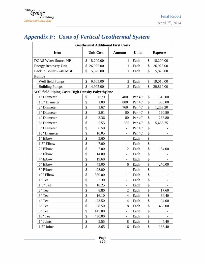
Final Report

April 7th, 2014

Page 129

Appendix F: Costs of Vertical Geothermal System


Item Unit Cost Amount Units Expense

DOAS Water Source HP $ 18,200.00 1 Each $ 18,200.00

Energy Recovery Unit $ 26,925.00 1 Each $ 26,925.00

Backup Boiler - 240 MBH $ 5,825.00 1 Each $ 5,825.00

Pumps

Well field Pumps $ 9,505.00 2 Each $ 19,010.00

Building Pumps $ 14,905.00 2 Each $ 29,810.00

Well field Piping Costs-High Density Polyethylene

1" Diameter $ 0.79 400 Per 40' $ 316.00

1.5" Diameter $ 1.00 800 Per 40' $ 800.00

2" Diameter $ 1.67 760 Per 40' $ 1,269.20

3" Diameter $ 2.01 80 Per 40' $ 160.80

4" Diameter $ 3.36 80 Per 40' $ 268.80

6" Diameter $ 5.55 985 Per 40' $ 5,466.75

8" Diameter $ 6.50 - Per 40' $ -

10" Diameter $ 10.05 - Per 40' $ -

1" Elbow $ 5.60 - Each $ -

1.5" Elbow $ 7.00 - Each $ -

2" Elbow $ 7.00 12 Each $ 84.00

3" Elbow $ 14.00 - Each $ -

4" Elbow $ 19.60 - Each $ -

6" Elbow $ 45.00 6 Each $ 270.00

8" Elbow $ 98.00 - Each $ -

10" Elbow $ 380.00 - Each $ -

1" Tee $ 7.30 - Each $ -

1.5" Tee $ 10.25 - Each $ -

2" Tee $ 8.80 2 Each $ 17.60

3" Tee $ 16.10 4 Each $ 64.40

4" Tee $ 23.50 4 Each $ 94.00

6" Tee $ 58.50 8 Each $ 468.00

8" Tee $ 145.00 - Each $ -

10" Tee $ 430.00 - Each $ -

1" Joints $ 5.55 8 Each $ 44.40

1.5" Joints $ 8.65 16 Each $ 138.40

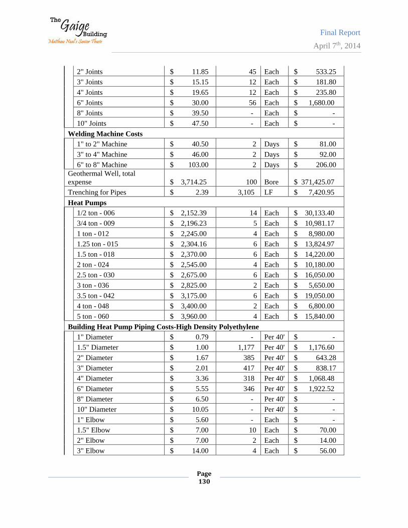
Final Report

April 7th, 2014

Page 130

2" Joints $ 11.85 45 Each $ 533.25

3" Joints $ 15.15 12 Each $ 181.80

4" Joints $ 19.65 12 Each $ 235.80

6" Joints $ 30.00 56 Each $ 1,680.00

8" Joints $ 39.50 - Each $ -

10" Joints $ 47.50 - Each $ -


1" to 2" Machine $ 40.50 2 Days $ 81.00

3" to 4" Machine $ 46.00 2 Days $ 92.00

6" to 8" Machine $ 103.00 2 Days $ 206.00

Geothermal Well, total

expense $ 3,714.25 100 Bore $ 371,425.07

Trenching for Pipes $ 2.39 3,105 LF $ 7,420.95

Heat Pumps

1/2 ton - 006 $ 2,152.39 14 Each $ 30,133.40

3/4 ton - 009 $ 2,196.23 5 Each $ 10,981.17

1 ton - 012 $ 2,245.00 4 Each $ 8,980.00

1.25 ton - 015 $ 2,304.16 6 Each $ 13,824.97

1.5 ton - 018 $ 2,370.00 6 Each $ 14,220.00

2 ton - 024 $ 2,545.00 4 Each $ 10,180.00

2.5 ton - 030 $ 2,675.00 6 Each $ 16,050.00

3 ton - 036 $ 2,825.00 2 Each $ 5,650.00

3.5 ton - 042 $ 3,175.00 6 Each $ 19,050.00

4 ton - 048 $ 3,400.00 2 Each $ 6,800.00

5 ton - 060 $ 3,960.00 4 Each $ 15,840.00

Building Heat Pump Piping Costs-High Density Polyethylene

1" Diameter $ 0.79 - Per 40' $ -

1.5" Diameter $ 1.00 1,177 Per 40' $ 1,176.60

2" Diameter $ 1.67 385 Per 40' $ 643.28

3" Diameter $ 2.01 417 Per 40' $ 838.17

4" Diameter $ 3.36 318 Per 40' $ 1,068.48

6" Diameter $ 5.55 346 Per 40' $ 1,922.52

8" Diameter $ 6.50 - Per 40' $ -

10" Diameter $ 10.05 - Per 40' $ -

1" Elbow $ 5.60 - Each $ -

1.5" Elbow $ 7.00 10 Each $ 70.00

2" Elbow $ 7.00 2 Each $ 14.00

3" Elbow $ 14.00 4 Each $ 56.00

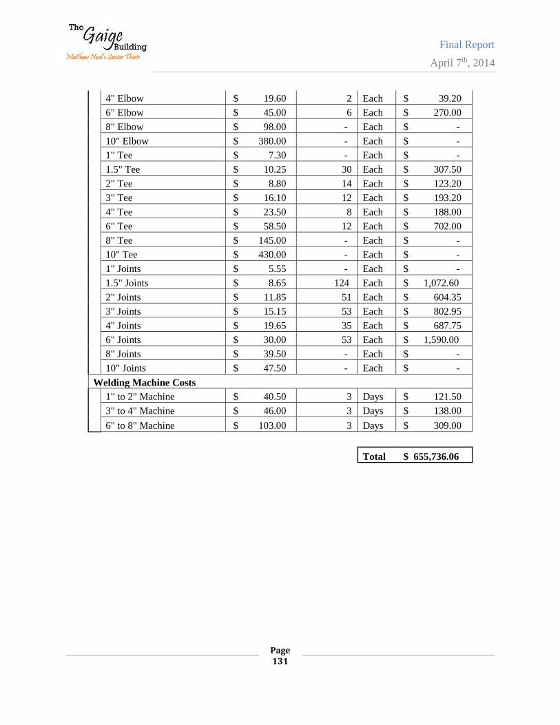
Final Report

April 7th, 2014

Page 131

4" Elbow $ 19.60 2 Each $ 39.20

6" Elbow $ 45.00 6 Each $ 270.00

8" Elbow $ 98.00 - Each $ -

10" Elbow $ 380.00 - Each $ -

1" Tee $ 7.30 - Each $ -

1.5" Tee $ 10.25 30 Each $ 307.50

2" Tee $ 8.80 14 Each $ 123.20

3" Tee $ 16.10 12 Each $ 193.20

4" Tee $ 23.50 8 Each $ 188.00

6" Tee $ 58.50 12 Each $ 702.00

8" Tee $ 145.00 - Each $ -

10" Tee $ 430.00 - Each $ -

1" Joints $ 5.55 - Each $ -

1.5" Joints $ 8.65 124 Each $ 1,072.60

2" Joints $ 11.85 51 Each $ 604.35

3" Joints $ 15.15 53 Each $ 802.95

4" Joints $ 19.65 35 Each $ 687.75

6" Joints $ 30.00 53 Each $ 1,590.00

8" Joints $ 39.50 - Each $ -

10" Joints $ 47.50 - Each $ -


1" to 2" Machine $ 40.50 3 Days $ 121.50

3" to 4" Machine $ 46.00 3 Days $ 138.00

6" to 8" Machine $ 103.00 3 Days $ 309.00

Total $ 655,736.06

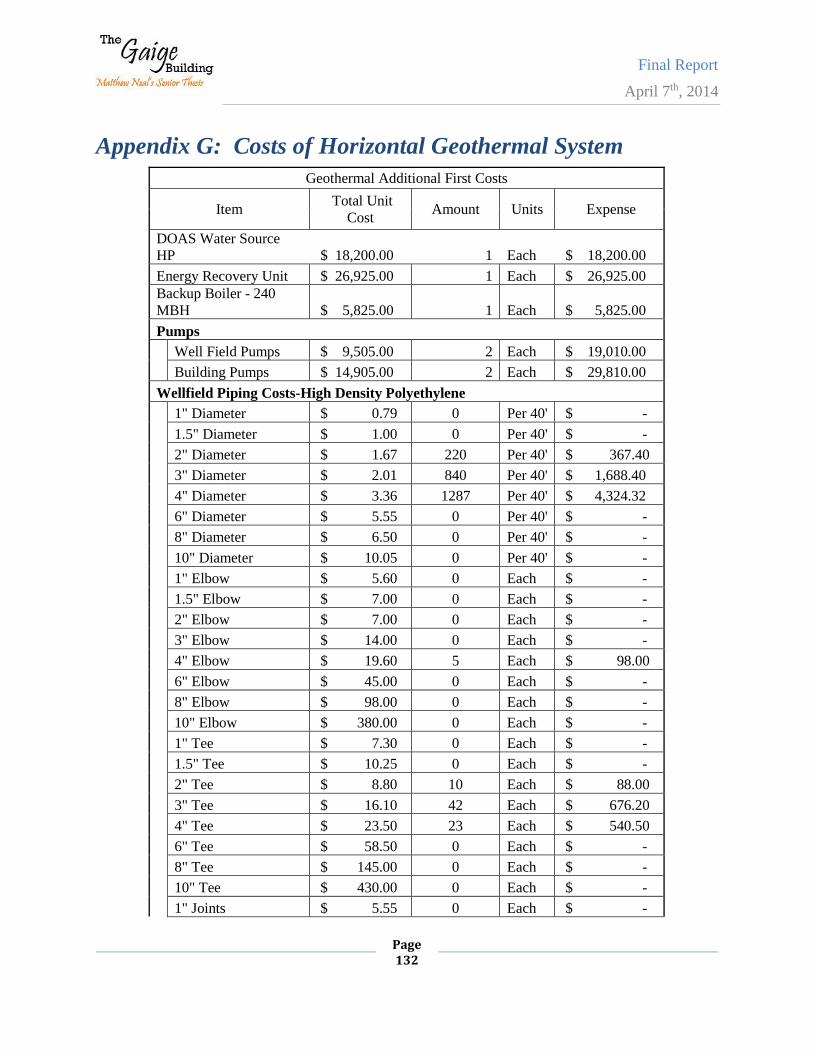
Final Report

April 7th, 2014

Page 132

Appendix G: Costs of Horizontal Geothermal System


Item Total Unit

Cost Amount Units Expense

DOAS Water Source

HP $ 18,200.00 1 Each $ 18,200.00

Energy Recovery Unit $ 26,925.00 1 Each $ 26,925.00

Backup Boiler - 240

MBH $ 5,825.00 1 Each $ 5,825.00

Pumps

Well Field Pumps $ 9,505.00 2 Each $ 19,010.00

Building Pumps $ 14,905.00 2 Each $ 29,810.00

Wellfield Piping Costs-High Density Polyethylene

1" Diameter $ 0.79 0 Per 40' $ -

1.5" Diameter $ 1.00 0 Per 40' $ -

2" Diameter $ 1.67 220 Per 40' $ 367.40

3" Diameter $ 2.01 840 Per 40' $ 1,688.40

4" Diameter $ 3.36 1287 Per 40' $ 4,324.32

6" Diameter $ 5.55 0 Per 40' $ -

8" Diameter $ 6.50 0 Per 40' $ -

10" Diameter $ 10.05 0 Per 40' $ -

1" Elbow $ 5.60 0 Each $ -

1.5" Elbow $ 7.00 0 Each $ -

2" Elbow $ 7.00 0 Each $ -

3" Elbow $ 14.00 0 Each $ -

4" Elbow $ 19.60 5 Each $ 98.00

6" Elbow $ 45.00 0 Each $ -

8" Elbow $ 98.00 0 Each $ -

10" Elbow $ 380.00 0 Each $ -

1" Tee $ 7.30 0 Each $ -

1.5" Tee $ 10.25 0 Each $ -

2" Tee $ 8.80 10 Each $ 88.00

3" Tee $ 16.10 42 Each $ 676.20

4" Tee $ 23.50 23 Each $ 540.50

6" Tee $ 58.50 0 Each $ -

8" Tee $ 145.00 0 Each $ -

10" Tee $ 430.00 0 Each $ -

1" Joints $ 5.55 0 Each $ -

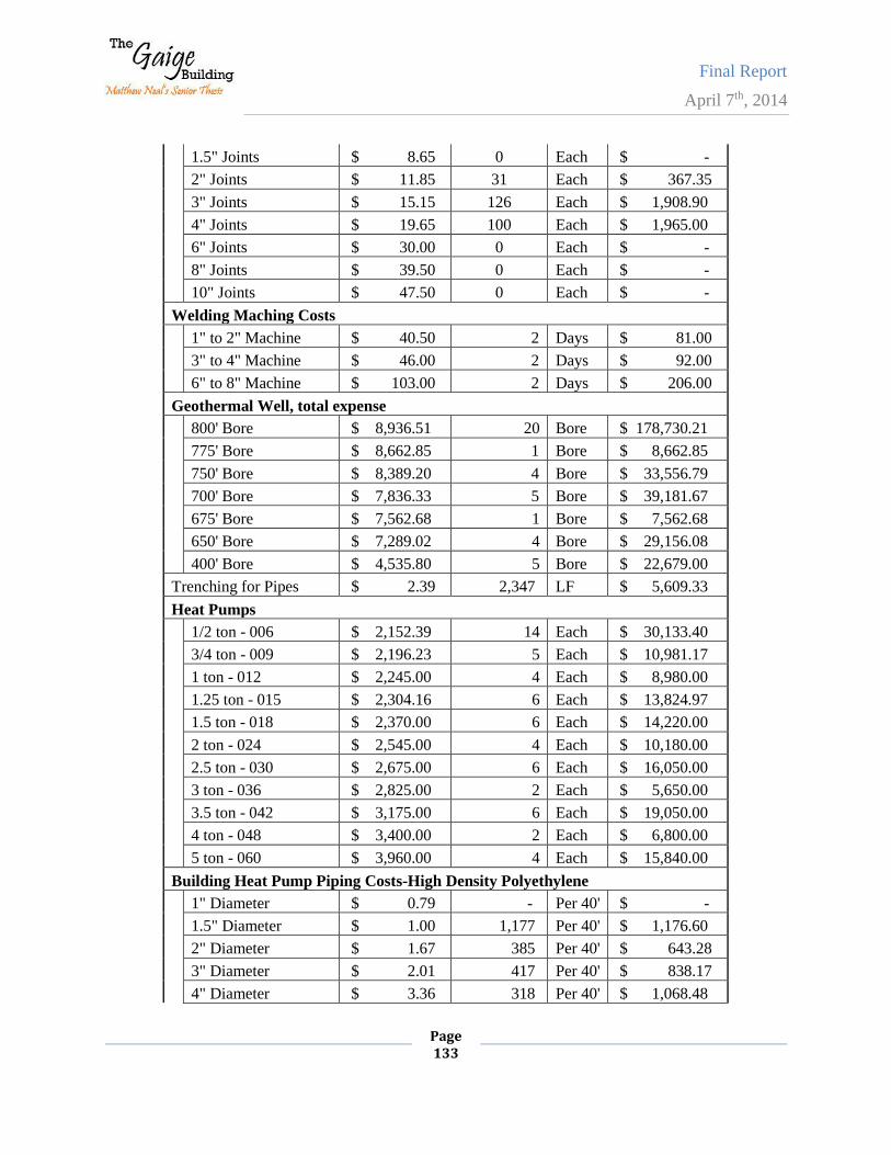
Final Report

April 7th, 2014

Page 133

1.5" Joints $ 8.65 0 Each $ -

2" Joints $ 11.85 31 Each $ 367.35

3" Joints $ 15.15 126 Each $ 1,908.90

4" Joints $ 19.65 100 Each $ 1,965.00

6" Joints $ 30.00 0 Each $ -

8" Joints $ 39.50 0 Each $ -

10" Joints $ 47.50 0 Each $ -

Welding Maching Costs

1" to 2" Machine $ 40.50 2 Days $ 81.00

3" to 4" Machine $ 46.00 2 Days $ 92.00

6" to 8" Machine $ 103.00 2 Days $ 206.00

Geothermal Well, total expense

800' Bore $ 8,936.51 20 Bore $ 178,730.21

775' Bore $ 8,662.85 1 Bore $ 8,662.85

750' Bore $ 8,389.20 4 Bore $ 33,556.79

700' Bore $ 7,836.33 5 Bore $ 39,181.67

675' Bore $ 7,562.68 1 Bore $ 7,562.68

650' Bore $ 7,289.02 4 Bore $ 29,156.08

400' Bore $ 4,535.80 5 Bore $ 22,679.00

Trenching for Pipes $ 2.39 2,347 LF $ 5,609.33

Heat Pumps

1/2 ton - 006 $ 2,152.39 14 Each $ 30,133.40

3/4 ton - 009 $ 2,196.23 5 Each $ 10,981.17

1 ton - 012 $ 2,245.00 4 Each $ 8,980.00

1.25 ton - 015 $ 2,304.16 6 Each $ 13,824.97

1.5 ton - 018 $ 2,370.00 6 Each $ 14,220.00

2 ton - 024 $ 2,545.00 4 Each $ 10,180.00

2.5 ton - 030 $ 2,675.00 6 Each $ 16,050.00

3 ton - 036 $ 2,825.00 2 Each $ 5,650.00

3.5 ton - 042 $ 3,175.00 6 Each $ 19,050.00

4 ton - 048 $ 3,400.00 2 Each $ 6,800.00

5 ton - 060 $ 3,960.00 4 Each $ 15,840.00

Building Heat Pump Piping Costs-High Density Polyethylene

1" Diameter $ 0.79 - Per 40' $ -

1.5" Diameter $ 1.00 1,177 Per 40' $ 1,176.60

2" Diameter $ 1.67 385 Per 40' $ 643.28

3" Diameter $ 2.01 417 Per 40' $ 838.17

4" Diameter $ 3.36 318 Per 40' $ 1,068.48

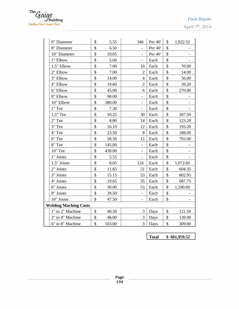
Final Report

April 7th, 2014

Page 134

6" Diameter $ 5.55 346 Per 40' $ 1,922.52

8" Diameter $ 6.50 - Per 40' $ -

10" Diameter $ 10.05 - Per 40' $ -

1" Elbow $ 5.60 - Each $ -

1.5" Elbow $ 7.00 10 Each $ 70.00

2" Elbow $ 7.00 2 Each $ 14.00

3" Elbow $ 14.00 4 Each $ 56.00

4" Elbow $ 19.60 2 Each $ 39.20

6" Elbow $ 45.00 6 Each $ 270.00

8" Elbow $ 98.00 - Each $ -

10" Elbow $ 380.00 - Each $ -

1" Tee $ 7.30 - Each $ -

1.5" Tee $ 10.25 30 Each $ 307.50

2" Tee $ 8.80 14 Each $ 123.20

3" Tee $ 16.10 12 Each $ 193.20

4" Tee $ 23.50 8 Each $ 188.00

6" Tee $ 58.50 12 Each $ 702.00

8" Tee $ 145.00 - Each $ -

10" Tee $ 430.00 - Each $ -

1" Joints $ 5.55 - Each $ -

1.5" Joints $ 8.65 124 Each $ 1,072.60

2" Joints $ 11.85 51 Each $ 604.35

3" Joints $ 15.15 53 Each $ 802.95

4" Joints $ 19.65 35 Each $ 687.75

6" Joints $ 30.00 53 Each $ 1,590.00

8" Joints $ 39.50 - Each $ -

10" Joints $ 47.50 - Each $ -

Welding Maching Costs

1" to 2" Machine $ 40.50 3 Days $ 121.50

3" to 4" Machine $ 46.00 3 Days $ 138.00

6" to 8" Machine $ 103.00 3 Days $ 309.00

Total $ 601,959.52

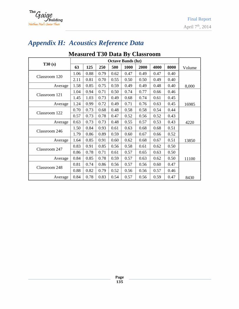
Final Report

April 7th, 2014

Page 135

Appendix H: Acoustics Reference Data

Measured T30 Data By Classroom

T30 (s) Octave Bands (hz)

Volume 63 125 250 500 1000 2000 4000 8000

Classroom 120 1.06 0.88 0.79 0.62 0.47 0.49 0.47 0.40

8,000

2.11 0.81 0.70 0.55 0.50 0.50 0.49 0.40

Average 1.58 0.85 0.75 0.59 0.49 0.49 0.48 0.40

Classroom 121 1.04 0.94 0.71 0.50 0.74 0.77 0.66 0.46

16985

1.45 1.03 0.73 0.49 0.68 0.74 0.61 0.45

Average 1.24 0.99 0.72 0.49 0.71 0.76 0.63 0.45

Classroom 122 0.70 0.73 0.68 0.48 0.58 0.58 0.54 0.44

4220

0.57 0.73 0.78 0.47 0.52 0.56 0.52 0.43

Average 0.63 0.73 0.73 0.48 0.55 0.57 0.53 0.43

Classroom 246 1.50 0.84 0.93 0.61 0.63 0.68 0.68 0.51

13850

1.79 0.86 0.89 0.59 0.60 0.67 0.66 0.52

Average 1.64 0.85 0.91 0.60 0.62 0.68 0.67 0.51

Classroom 247 0.83 0.91 0.85 0.56 0.58 0.61 0.62 0.50

11100

0.86 0.78 0.71 0.61 0.57 0.65 0.63 0.50

Average 0.84 0.85 0.78 0.59 0.57 0.63 0.62 0.50

Classroom 248 0.81 0.74 0.86 0.56 0.57 0.56 0.60 0.47

8430

0.88 0.82 0.79 0.52 0.56 0.56 0.57 0.46

Average 0.84 0.78 0.83 0.54 0.57 0.56 0.59 0.47

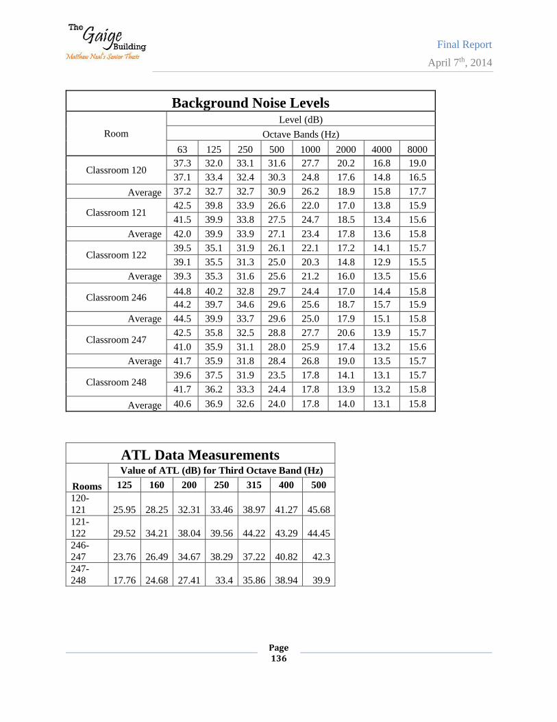
Final Report

April 7th, 2014

Page 136

Background Noise Levels

Room

Level (dB)

Octave Bands (Hz)

63 125 250 500 1000 2000 4000 8000

Classroom 120 37.3 32.0 33.1 31.6 27.7 20.2 16.8 19.0

37.1 33.4 32.4 30.3 24.8 17.6 14.8 16.5

Average 37.2 32.7 32.7 30.9 26.2 18.9 15.8 17.7

Classroom 121 42.5 39.8 33.9 26.6 22.0 17.0 13.8 15.9

41.5 39.9 33.8 27.5 24.7 18.5 13.4 15.6

Average 42.0 39.9 33.9 27.1 23.4 17.8 13.6 15.8

Classroom 122 39.5 35.1 31.9 26.1 22.1 17.2 14.1 15.7

39.1 35.5 31.3 25.0 20.3 14.8 12.9 15.5

Average 39.3 35.3 31.6 25.6 21.2 16.0 13.5 15.6

Classroom 246 44.8 40.2 32.8 29.7 24.4 17.0 14.4 15.8

44.2 39.7 34.6 29.6 25.6 18.7 15.7 15.9

Average 44.5 39.9 33.7 29.6 25.0 17.9 15.1 15.8

Classroom 247 42.5 35.8 32.5 28.8 27.7 20.6 13.9 15.7

41.0 35.9 31.1 28.0 25.9 17.4 13.2 15.6

Average 41.7 35.9 31.8 28.4 26.8 19.0 13.5 15.7

Classroom 248 39.6 37.5 31.9 23.5 17.8 14.1 13.1 15.7

41.7 36.2 33.3 24.4 17.8 13.9 13.2 15.8

Average 40.6 36.9 32.6 24.0 17.8 14.0 13.1 15.8

ATL Data Measurements

Rooms

Value of ATL (dB) for Third Octave Band (Hz)

125 160 200 250 315 400 500

120-

121 25.95 28.25 32.31 33.46 38.97 41.27 45.68

121-

122 29.52 34.21 38.04 39.56 44.22 43.29 44.45

246-

247 23.76 26.49 34.67 38.29 37.22 40.82 42.3

247-

248 17.76 24.68 27.41 33.4 35.86 38.94 39.9

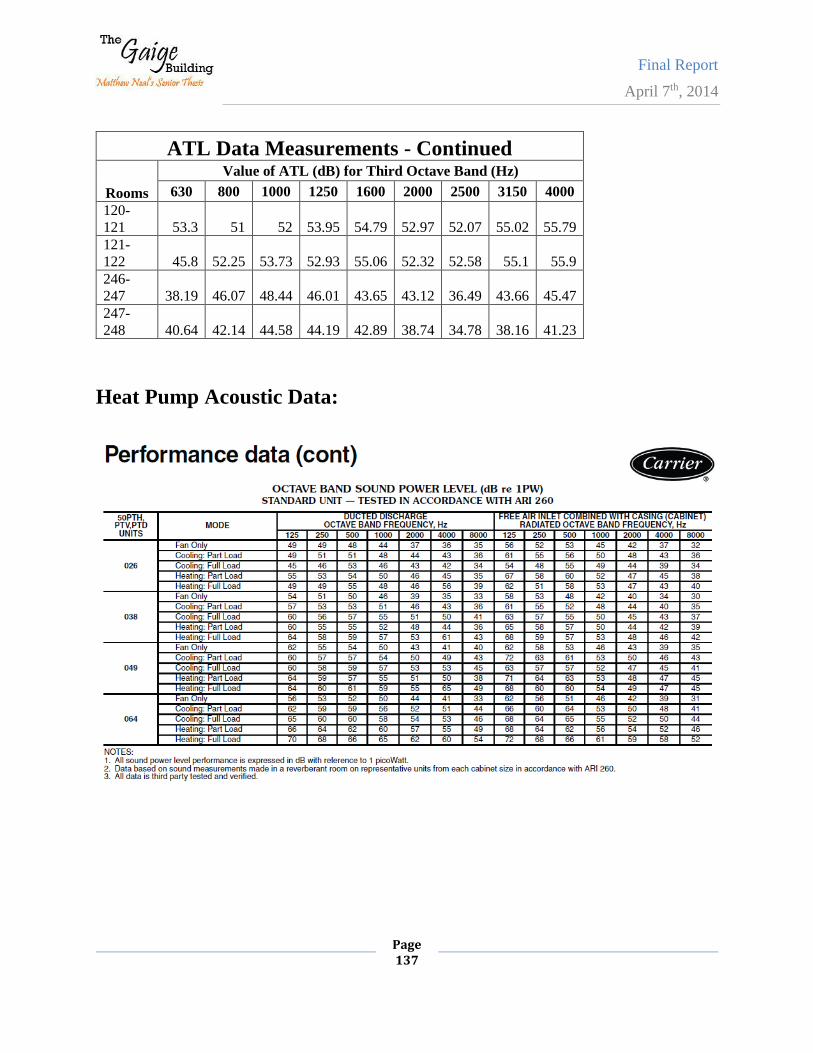
Final Report

April 7th, 2014

Page 137

ATL Data Measurements - Continued

Rooms

Value of ATL (dB) for Third Octave Band (Hz)

630 800 1000 1250 1600 2000 2500 3150 4000

120-

121 53.3 51 52 53.95 54.79 52.97 52.07 55.02 55.79

121-

122 45.8 52.25 53.73 52.93 55.06 52.32 52.58 55.1 55.9

246-

247 38.19 46.07 48.44 46.01 43.65 43.12 36.49 43.66 45.47

247-

248 40.64 42.14 44.58 44.19 42.89 38.74 34.78 38.16 41.23

Heat Pump Acoustic Data:

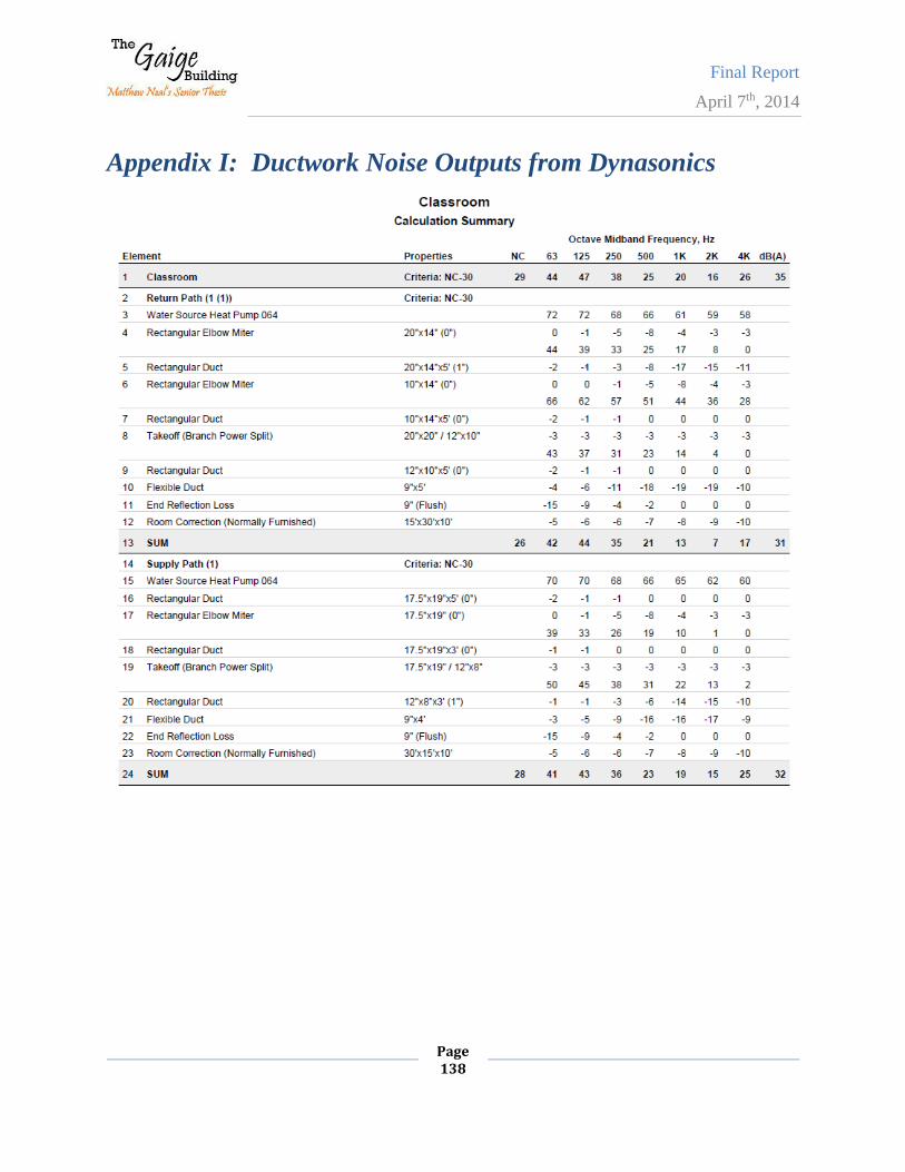
Final Report

April 7th, 2014

Page 138

Appendix I: Ductwork Noise Outputs from Dynasonics

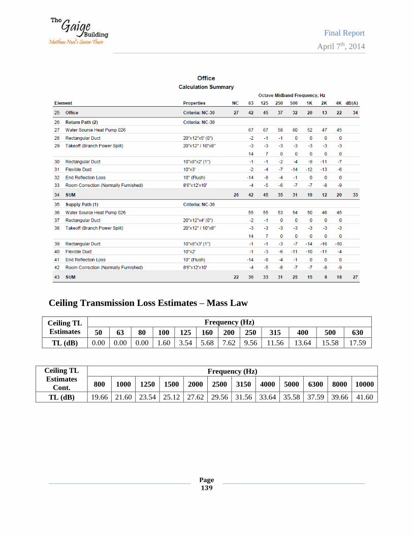
Final Report

April 7th, 2014

Page 139

Ceiling Transmission Loss Estimates – Mass Law

Ceiling TL

Estimates

Frequency (Hz)

50 63 80 100 125 160 200 250 315 400 500 630

TL (dB) 0.00 0.00 0.00 1.60 3.54 5.68 7.62 9.56 11.56 13.64 15.58 17.59

Ceiling TL

Estimates

Cont.

Frequency (Hz)

800 1000 1250 1500 2000 2500 3150 4000 5000 6300 8000 10000

TL (dB) 19.66 21.60 23.54 25.12 27.62 29.56 31.56 33.64 35.58 37.59 39.66 41.60

Final Report

April 7th, 2014

Page 140

Academic Vita Matthew T. Neal

5125 Redwood Drive

Indiana, PA 15701

[email protected]

Education Combined Masters of Science and Bachelor of Architectural Engineering Mechanical Option

The Pennsylvania State University, Schreyer Honors College

Graduating Class of 2014 (BAE) and 2015 (MS)

Relevant

Coursework Advanced Architectural Acoustics, Fundamentals of Acoustics, Acoustics in a

Fluid Media, 2012 Rome Study Abroad Program, Advanced HVAC,

Thermodynamics, Structural Analysis, Fundamentals of HVAC, Fundamentals

of Electrical Systems, Architectural Design Studio coursework

Work Experience Research Experience for Undergraduates May 2013 to Sept. 2013

The Applied Research Lab, Penn State University Park, PA

Performed a literature review of background research

Created and validated a computer model of a 2000 seat concert hall

Conducted subjective studies on concert hall acoustics

Student Researcher July 2012 to August 2012

The Applied Research Lab, Penn State University Park, PA

Gathered, processed, analyzed, and presented acoustical data

Measured acoustical properties of thermo-acoustic speakers

Mechanical / HVAC Intern May 2011 to August 2011

H. F. Lenz Company Johnstown, PA

Developed mechanical equipment within Revit MEP

Calculated ventilation requirements and heating loads

Presentations “The effect of using matched, but not individualized, head related transfer

functions on the subjective evaluation of auralizations” Neal & Vigeant

Acoustical Society of America Meeting, San Francisco – December 2nd, 2013

Activities Essence of Joy, Treasurer Fall 2009 to Present

The Navigators, Bible Study Leader Fall 2009 to Present

Acoustical Society of America Fall 2013 to Present

Awards & Honors AE Alumni Association Scholarship Spring 2011

Dean’s List Fall 2009 to Fall 2012

AE General Scholarship Spring 2012

Tau Beta Pi Engineering Honor Society Fall 2011 to Present0

TheGaige - Pennsylvania State University

Documents

Transcript of TheGaige - Pennsylvania State University