The Wisconsin Hydrology H - The Learning Storelearningstore.uwex.edu/assets/pdfs/g3691-2.pdf ·...

1

HydrologyWisconsin

M A N U A L

The

Storm Water

G3691-2

Hydrology is the study of the move-ment of water through the envi-ronment. We refer to water�s

movement from the atmospherethrough the earth and back to theatmosphere as the hydrologic cycle. Inthis manual, we restrict the discussionof hydrology to those portions of thecycle that affect stormwater manage-ment and water quality�precipitation,runoff and infiltration. For an overviewof storm water hydrology and howurbanization affects surface waterrunoff, refer to the Wisconsin StormWater Manual, Part 1 (Prey, 1994).

Water quality criteriaCertain hydrologic methods for sizingstorm water management practices (forexample, grassed swales, infiltrationstructures and wet detention basins)accomplish two goals:

1. To remove a pollutant to a desiredperformance standard. For example,a widely accepted standard is toremove a minimum of 80% of thetotal suspended solids generatedfrom the tributary drainage area onan average annual basis. AWisconsin Department of NaturalResources (DNR) study has estab-lished that this level of performancecan be achieved in urban areas bydesigning for removal of the 5-micron particle from runoff from a1.5-inch, 4-hour rainfall event. (WI-DNR, 1997)

2. To control runoff peak or volume toa desired design level for waterquality management. While man-agement practices aimed primarilyat water quality management mayalso have flood control objectives,this manual does not address flowcontrol for storms greater than the2-year rainfall and, therefore, doesnot address practices associatedwith flood control. Contact the U. S.Department of Agriculture-NaturalResources Conservation Service(NRCS), the Army Corps ofEngineers or seek other sources forguidance on flood control concerns.

Design processoverviewTo size water quality management prac-tices, the Small Storm Hydrology methodhas been used to predict the runoff froma 1.5-inch, 4-hour rainfall. This method,developed by Pitt and explained in SmallStorm Hydrology: The Integration of Flowwith Water Quality Management Practices(Pitt, 1989), is used to predict runoff fromsmall storms and areas with short con-centration times.

To determine the management practicestorage volume and peak dischargefrom the 2-year, 24-hour storm, themethod described in Urban Hydrologyfor Small Watersheds, Technical Release 55(USDA-SCS, 1986) is used.

The water quality design process usesthe drainage area�s hydrologic charac-teristics to determine the design runoff.After assessing the site data and water-shed characteristics, the managementpractice is designed. A brief overviewof the recommended design procedure

Numerous methods are used to

predict runoff peaks and

volumes and routing flows (See

for example Pitt, 1989; USDA-

SCS, 1986; Walker, 1990). Two

commonly used methods, Small

Storm Hydrology and TR 55, are

described in this manual for illus-

trative purposes. Check with

local or state codes to determine

if specific methods and storm

events have been prescribed for

your location.

2

W I S C O N S I N S T O R M W A T E R M A N U A L _______________________________________________________________________________

is given below to assist the reader inunderstanding the overall process. Notall steps may be necessary for everydesign. A more detailed description,along with an example, is presentedlater in this section of the manual.

The steps in the design process forwater quality management practices areas follows.

Step 1. Before design begins, thedesigner should consult with localofficials, regional planning agenciesand the DNR regional office to deter-mine zoning restrictions, watershedrequirements and/or surface andgroundwater requirements that mayapply to the development site orwatershed. Local ordinances andstate codes should also be checked todetermine if design storm designa-tions and prediction methods havebeen prescribed.

Step 2. Determine the viability ofvarious water quality practices bycollecting and analyzing watersheddata and site characteristics usingscreening criteria such as those con-tained in the introductory section ofthis manual.

Step 3. Calculate the expected runoffvolume from the developeddrainage area for the design storms.Two design storms are consideredhere. A 1.5-inch, 4-hour storm isused for water quality control andthe 2-year, 24-hour storm is used forflow control at bank full conditions.

Step 4. Create hydrographs for thedrainage area for the water qualitycontrol design rainfall and the bankfull conditions. These hydrographsbecome the inflow hydrograph fordesign. If the structure is to be usedfor flood control, the designer mayalso want to develop hydrographsfor additional storms at this time.These hydrographs may be requiredfor flow routing purposes later inthe design process.

Step 5. From the information gatheredfrom steps 1�4 above, select thewater quality management prac-tice(s) that is/are best suited to thedrainage area and the managementgoals.

Step 6. Develop a preliminary man-agement practice design for thedesign storm.

Step 7. For those practices that requirerouting, route the design hydro-graph through the structure as acheck of the water quality dischargeand runoff storage requirements. Ifthe water quality criteria are not sat-isfied, or the structure is excessivelylarge, repeat step 6 and redesign thestructure to correct design flaws.Recheck the design and repeat thisloop as required.

Step 8. If not previously determinedas a part of step 4, determine thepeak discharge for the drainage areain its existing condition and developthe 2-year, 24-hour hydrographusing the tabular method from TR-55 Urban Hydrology for SmallWatersheds (USDA-SCS, 1986).

Step 9. Develop a preliminary designthat limits the post-developed peakdischarge to the pre-developed peakdischarge for the 2-year, 24-hourrain event or to the peak as pre-scribed in local ordinances incorpo-rating management practice designfor water quality control.

Step 10. Route the 2-year, 24-hourrainfall hydrograph from the devel-oped area through the managementpractice to check that the practicemeets the peak flow and runoffstorage requirements. If the peakdischarge from the managementpractice exceeds the pre-developedpeak discharge, or if the structure isexcessively large, return to step 8and redesign the structure to correctthe design flaws. Repeat steps 8, 9and 10 as required.

Step 11. Design and route othercontrol discharges as needed. Somemanagement practices, such as infil-tration basins and trenches, may nothandle flows above the 2-year, 24-hour storm. In such cases, largerflows will need to be divertedaround the practice.

Step 12. Assess the effects on thewatershed and stream for flowsexpected after the installation of themanagement practice.

Step 13. Design details of the manage-ment practice, including safety, main-tenance and operational features.

Step 14. Develop plans and specifica-tions for the design and construc-tion of the management practice anda maintenance plan.

Hydrologic principles for thedesign of waterquality managementpractices

Precipitation is the driving forcein the hydrologic cycle. Duringsome rainfall events, all precipi-

tation is either intercepted by vegetationor infiltrated into the soil. In such casesno surface runoff occurs. However,when rainfall or snowmelt exceeds thesoil�s infiltration rate, excess waterbegins to accumulate as surface storagein small topographic depressions. As thedepth of water in surface detentionincreases, overland flow may occur.Overland flow quickly concentrates intosmall rills or channels, which then flowinto larger streams.

Rainfall can also infiltrate into the soiland move laterally through upper soilzones until it again appears on the soilsurface or enters a stream channel. Thisshallow lateral flow is known as inter-flow. A portion of the precipitation maypercolate to the water table. Percolationwill contribute to stream base flow ifthe water table intersects the streamchannel.

3

_____________________________________________________________________________________________________________________ H Y D R O L O G Y

Factors such as antecedent soil mois-ture, surface cover, variable infiltrationrate and seasonal variations make thedevelopment of rainfall-runoff relation-ships difficult. Although a number ofmethods to calculate runoff from aknown rainfall event have been devel-oped, these methods must be used withcaution. The advantages, disadvantagesand limitations of each method shouldbe known if an appropriate modelchoice is to be made.

Computation methodThe storm water components of concernin this manual are the water qualitycomponent and the peak dischargereduction necessary to protect streambanks and stream biota from increasedrunoff due to urbanization. Runoffvolume is usually the most importanthydrologic parameter in design of man-agement practices for water quality,while peak flow discharge and time ofconcentration are the most importanthydrologic parameters for flood control.Runoff models for water quality investi-gations, therefore, may differ fromrunoff models for flood control.

The storms to be assessed from a waterquality concern are high frequencystorms of relatively small magnitude.These small storms are responsible forthe majority of the pollutant loads gen-erated from urban areas on an annualbasis (EPA 1983, Pitt 1989). For �bankfull� conditions, peak discharge fromthe 2-year, 24-hour storm from thedrainage area in a fully developed con-dition should be limited to the peak dis-charge from a 2-year, 24-hour storm inthe pre-developed condition, or to thelevel specified in local ordinances.

Models other than those described inthis manual may be applicable. Thedesigner is encouraged to explore avariety of models to determine thosemost appropriate for the situation, pro-vided local regulations allow their use.Most models are for single event designstorms. Continuous simulation models

(for example, see Bicknell et. al., 1997)are alternatives for assessing the pollu-tant removal efficiency of managementpractices. These models typically use anannual rainfall event file and analyzepollutant loading and runoff volumefrom a specified rain file on a givenland-use. Pollutant loads are thensummed on a mass basis and a theoret-ical removal rate calculated. The com-plexity of these simulation modelsrequires that a computer be used in theassessment.

Water quality—smallstorm hydrologyTo simplify the management practicedesign process for water quality control,a single event approach will be dis-cussed in this document. For purposesof illustration, the runoff volume pro-duced by the 1.5-inch storm is used. Bytreating all runoff from storms up toand including the 1.5-inch design stormsize, a storm water management prac-tice should achieve approximately 80%removal of the annual total suspendedsolids loading delivered to that practice.By using the 1.5-inch storm, thedesigner can estimate the design runoffvolume and the required storagevolume to size controls. Water qualitypeak flow should not be confused withthe 2-year, 24-hour peak used for dis-charge rate control for bank full flowcontrol.

Some management practice situationsrequire the use of a flow splittingdevice. For example, a flow splittermight be required for an off-line man-agement practice when retrofittingpractices in an existing developed area.The hydraulic design flow for an off-line water quality management practicewould be determined using the 1.5-inchdesign storm and a 4-hour duration inconcert with a triangular hydrographmethod to calculate water quality peakflow. The splitter would then be used tobypass the remaining flow.

Water quality runoffvolumeTo estimate storm runoff volumes, peakflows and hydrographs for smallstorms, the Small Storm Hydrologymethod devised by Pitt (1989) is usedhere. This method uses volumetricrunoff coefficients to calculate runofffrom urban land-uses for small rainfalls.

The method is particularly useful indescribing the contributions of indi-vidual source areas to the total runoff orthe effectiveness of individual sourcearea controls. Land development char-acteristics (landscaping, streets,drainage system type, etc.) are usuallycritical when determining small-stormflows and the variable urban sourceareas contributing pollutants.

The volumetric runoff coefficients, Rv,in small storm hydrology are calibratedto account for various rainfall depths.Small rains tend to have small volu-metric runoff coefficients that increaseas the rainfall depths increase. Perviousareas are less responsive to rainfalldepths than mostly impervious areas.The approach used in calculating thewater quality volume is to establish theRv values and runoff volumes from thevarious source areas for the design rain-fall. Source areas considered are consis-tent with those used in the SourceLoading and Management Model(SLAMM) computer model (Pitt, 1994).Six different land use types defined intable 1.

Calculation of the design runoff volumefrom a watershed uses the area, theweighted volumetric runoff coefficientsfor various source areas (table 2) for the1.5-inch storm, the individual land usesource areas, and a conversion factor toconvert acre-inches into acre-feet. If thedesign rainfall is different than 1.5inches, the runoff coefficients must beadjusted as in Pitt (1989).

Land use runoff volume (cu.ft.) = (1.5 in)(1 ft/12 in)(Rv)(43560sq.ft/ac)(Area acres)

4


Table 1. Land use and pollutant source area definitions

Residential land uses■ High Density Residential without Alleys (HRNA): Urban single family housing at a density of greater than 6 units/acre.

Includes house, driveway, yard and streets.

■ High Density Residential with Alleys (HRWA): Same as HRNA except alleys exist behind the houses where the backyards join.

■ Medium Density without Alleys (MRNA): Same as HRNA except the density is between 2-6 units/acre.

■ Medium Density with Alleys (MRNA): Same as HRWA except alleys exist behind the houses where the back yards join.

■ Low Density (LR) : Same as HRNA except the density is 0.7 to 2 units/acre.

■ Multiple Family (MF): Housing for three or more family units from 1-3 stories in height. Units may be adjoined up-and-down, side-by-side or front-and-rear. Includes building, yard, parking lot and driveways.

■ High Rise (HIR): Same as MF except buildings are apartments 4 or more stories in height.

■ Trailer Parks (MOBR): For a mobile home or trailer park, includes all vehicle homes, the yard, driveway and office area.

■ Suburban (SUBR): Same as HRNA except the density is between 0.2 and 0.6 units/acre.

Commercial land uses■ Strip Commercial (CST): Those buildings for which the primary function involves the sale of goods or services. This cate-

gory includes some institutional lands found in commercial strips, such as post offices, court houses and fire and policestations. This category does not include buildings used for the manufacture of goods or warehouses. This land useincludes the buildings, parking lots and streets. It does not include nursery, tree farms or lumberyards.

■ Shopping Centers (SC): Commercial areas where the related parking lot is at least 2.5 times the area of the buildings� roofarea. The buildings in this land use are usually surrounded by the parking area. This land use includes the buildings,parking lot and the streets.

■ Office Parks (OP): Land use where non-retail business takes place. The buildings are usually multi-story, surrounded bylarger areas of lawn and other landscaping. This land use includes the buildings, lawn and road areas. Establishmentsthat may be in this category include: insurance offices, government buildings and company headquarters.

■ Downtown Commercial (CDT): Highly impervious downtown areas of commercial and institutional land use.

Industrial land uses■ Manufacturing (MI): Those buildings and premises devoted to the manufacture of products. This category includes utility

power plants.

■ Non-Manufacturing (LI): Those buildings used for the storage and/or distribution of goods awaiting further processingor sale to retailers. This category includes warehouses and wholesalers. This category also includes businesses such aslumberyards, auto salvage yards, junk yards, oil tank farms, coal and salt storage areas, grain elevators, agriculturalcoops and areas for bulk storage of fertilizers and pesticides.

Institutional land uses■ Hospitals (HOSP): Medical facilities that provide inpatient overnight care. Includes nursing homes, state, county or

private facilities. Includes buildings, grounds, parking lots and drives.

■ Education (SCH): Includes any public or private primary, secondary, or college educational institutional grounds.Includes buildings, playgrounds, athletic fields, roads, parking lots and lawn areas.

■ Miscellaneous Institutional (MISC): Churches and large areas of institutional property not part of CST and CDT.

Open space land uses■ Cemeteries (CEM): Includes cemetery grounds, roads, and buildings located on the grounds.

■ Parks (PARK): Outdoor recreational areas including municipal playgrounds, botanical gardens, arboretums, golf coursesand natural areas.

■ Undeveloped (OSUD) : Lands that are private or publicly owned with no structures and have a complete vegetative cover.This includes vacant lots, transformer stations, radio and TV transmission areas, water towers and railroad rights-of-way.

Freeway land uses■ Freeways (FREE): Limited access highways and the interchange areas.

5

_____________________________________________________________________________________________________________________ H Y D R O L O G Y

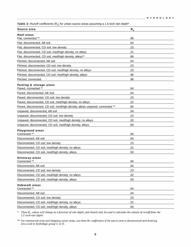
Table 2: Runoff coefficients (Rv) for urban source areas assuming a 1.5-inch rain depth*

Source area Rv

Roof areasFlat, connected ** .88

Flat, disconnected, AB soil .04

Flat, disconnected, CD soil, low density .23

Flat, disconnected, CD soil, med/high density, no alleys .21

Flat, disconnected, CD soil, med/high density, alleys** .86

Pitched, disconnected, AB soil .04

Pitched, disconnected, CD soil, low density .23

Pitched, disconnected, CD soil, med/high density, no alleys .23

Pitched, disconnected, CD soil, med/high density, alleys .96

Pitched, connected .98

Parking & storage areasPaved, connected ** .94

Paved, disconnected, AB Soil .04

Paved, disconnected, CD soil, low density .23

Paved, disconnected, CD soil, med/high density, no alleys .22

Paved, disconnected, CD soil, med/high density, alleys unpaved, connected ** .85

Unpaved, disconnected, AB soil .04

Unpaved, disconnected, CD soil, low density .23

Unpaved, disconnected, CD soil, med/high density, no alleys .20

Unpaved, disconnected, CD soil, med/high density, alleys .84

Playground areasConnected ** .94

Disconnected, AB soil .04

Disconnected, CD soil, low density .23

Disconnected, CD soil, med/high density, no alleys .22

Disconnected, CD soil, med/high density, alleys .93

Driveway areasConnected ** .94





Sidewalk areasConnected ** .94





* These Rv values will change as a function of rain depth, and should only be used to calculate the volume of runoff from the 1.5 inch-rain depth.

** For commercial strip and shopping center areas, use these Rv coefficients if the source area is disconnected and draining into a soil in hydrologic group C or D.

6


Source area Rv

Street and alley areasSmooth texture ** .84

Intermediate texture ** .79

Rough texture ** .79

Very rough texture** .79

Landscaped areasLarge area, AB soil .04

Large area, CD soil .23

Small area, AB soil .04

Small area, CD soil .23

Undeveloped areasUndeveloped area, AB soil .04

Undeveloped area, CD soil .23

Other areasDirectly connected ** .94

Pervious, AB soil .04

Pervious, CD soil .23

Partially connected, AB soil .04

Partially connected, CD soil, low density .23

Partially connected, CD soil, med/high density, no alleys .22

Partially connected, CD soil, med/high density, alleys .93

Freeway areasPaved land & shoulder, smooth .84

Paved land & shoulder, intermediate .78

Paved land & shoulder, rough .78

Paved land & shoulder, very rough .78

Large turf area, AB soil .04

Large turf area, CD soil .23

Undeveloped area, AB soil .04

Undeveloped area, CD soil .23

Other directly connected areas ** .94

Partially connected, AB soil .04

Partially connected, CD soil, low density .23

Partially connected, CD soil, med/high density, no alleys .22

Partially connected, CD soil, med/high density, alleys .93

* These Rv values will change as a function of rain depth, and should only be used to calculate the volume of runoff from the 1.5 inch-rain depth.

** For commercial strip and shopping center areas, use these Rv coefficients if the source area is disconnected and draining into a soil in hydrologic group C or D.

7

_____________________________________________________________________________________________________________________ H Y D R O L O G Y

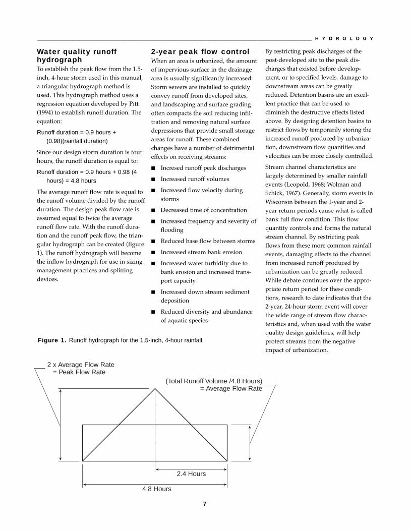
Water quality runoff hydrographTo establish the peak flow from the 1.5-inch, 4-hour storm used in this manual,a triangular hydrograph method isused. This hydrograph method uses aregression equation developed by Pitt(1994) to establish runoff duration. Theequation:

Runoff duration = 0.9 hours +(0.98)(rainfall duration)

Since our design storm duration is fourhours, the runoff duration is equal to:

Runoff duration = 0.9 hours + 0.98 (4hours) = 4.8 hours

The average runoff flow rate is equal tothe runoff volume divided by the runoffduration. The design peak flow rate isassumed equal to twice the averagerunoff flow rate. With the runoff dura-tion and the runoff peak flow, the trian-gular hydrograph can be created (figure1). The runoff hydrograph will becomethe inflow hydrograph for use in sizingmanagement practices and splittingdevices.

2-year peak flow controlWhen an area is urbanized, the amountof impervious surface in the drainagearea is usually significantly increased.Storm sewers are installed to quicklyconvey runoff from developed sites,and landscaping and surface gradingoften compacts the soil reducing infil-tration and removing natural surfacedepressions that provide small storageareas for runoff. These combinedchanges have a number of detrimentaleffects on receiving streams:

■ Incresed runoff peak discharges

■ Increased runoff volumes

■ Increased flow velocity duringstorms

■ Decreased time of concentration

■ Increased frequency and severity offlooding

■ Reduced base flow between storms

■ Increased stream bank erosion

■ Increased water turbidity due tobank erosion and increased trans-port capacity

■ Increased down stream sedimentdeposition

■ Reduced diversity and abundanceof aquatic species

By restricting peak discharges of thepost-developed site to the peak dis-charges that existed before develop-ment, or to specified levels, damage todownstream areas can be greatlyreduced. Detention basins are an excel-lent practice that can be used todiminish the destructive effects listedabove. By designing detention basins torestrict flows by temporarily storing theincreased runoff produced by urbaniza-tion, downstream flow quantities andvelocities can be more closely controlled.

Stream channel characteristics arelargely determined by smaller rainfallevents (Leopold, 1968; Wolman andSchick, 1967). Generally, storm events inWisconsin between the 1-year and 2-year return periods cause what is calledbank full flow condition. This flowquantity controls and forms the naturalstream channel. By restricting peakflows from these more common rainfallevents, damaging effects to the channelfrom increased runoff produced byurbanization can be greatly reduced.While debate continues over the appro-priate return period for these condi-tions, research to date indicates that the2-year, 24-hour storm event will coverthe wide range of stream flow charac-teristics and, when used with the waterquality design guidelines, will helpprotect streams from the negativeimpact of urbanization.

2.4 Hours

4.8 Hours

2 x Average Flow Rate = Peak Flow Rate

(Total Runoff Volume /4.8 Hours) = Average Flow Rate

Figure 1. Runoff hydrograph for the 1.5-inch, 4-hour rainfall.

8


Peak flow limitations warrant concernwhen streams or water bodies areaffected negatively by increased flows.Water bodies that experience only negli-gible effects from increased flow maynot have to conform to these guidelines.For example, increased flows fromsmall tributaries to a large lake such asLake Michigan would have little or noeffect on the lake�s water quality.

As mentioned earlier, the designmethod used to size management prac-tices to limit the 2-year, 24-hour peakflow from developing areas to the pre-developed peak flow is described in theNRCS TR-55 manual, Urban Hydrologyfor Small Watersheds (USDA-SCS, 1986).Because flow routing is used to prop-erly size stormwater management prac-tices, the tabular hydrograph methoddescribed in Urban Hydrology for SmallWatersheds is illustrated in this manual.Because numerous documents arereadily available and the calculationprocedure is commonly known,detailed coverage is not given here.However, an example demonstratingthe use of this procedure is given below.Contact the NRCS to obtain a copy ofthe TR-55 manual.

Structural storagevolume—flow routingThe design active storage volume is thevolume in the reservoir available toaccommodate the runoff from thedesign storms. The storage volumerequired is the difference between theinflow and outflow hydrographs asillustrated in figure 2. To determine thestorage volume needed, flow routingprocedures should be employed.

A management practice design is sub-jected to the expected inflow hydro-graph, and the storage and dischargeare analyzed to determine if the storagerequired exceeds the available storagevolume and if the outlet is properlysized. For water quality considerations,this method is used to develop, test andmodify the design to remove 80% of thetotal suspended solids in storm waterrunoff on an annual average basis.

Wisconsin DNR studies indicate thatremoval of the 5-micron particle fromrunoff from a 1.5-inch, 4-hour stormwill achieve 80% removal on an averageannual basis. Flow routing is also usedto develop, test and modify the basinstorage volume and outlet design forthe active storage for larger storms forbank full or peak control. The flowrouting method used in this manual isbased on the NRCS Technical Release-20 (USDA-SCS, 1992) as presented byMcCuen (1982). An example of this pro-cedure using a detention basin as amanagement practice follows.

Water quality management practice design: an example

The remainder of this section of thestorm water manual consists of adetailed example of a procedure for

designing a water quality managementpractice.

In this example, note that all runoffvalues and field data information, whilein the range of acceptable values, areassumed. The designer is responsiblefor collecting relevant field survey dataneeded to develop the basin design.Failure to collect survey data relevant tothe site characteristics will likely resultin designs that fail to meet design speci-fications and could result in a majorfailure of the basin facility. Theapproach given below is an example ofwhat could be done, but may not fitevery situation. Often design becomesan iterative process where the designevolves as more information is obtainedand alterations correct earlier designassumptions.

Time

Flo

w R

ate

Time Where Inflow = Outflow

Outflow Hydrograph

Storage Volume

Inflow Hydrograph

Figure 2. Flow difference between inflow and outflow hydrographs.

Adapted from Barfield et al. 1983.

9

_____________________________________________________________________________________________________________________ H Y D R O L O G Y

Steps 1 & 2 Inventory

Assume that the first two steps of thedesign process have been completed.The steps consist of: 1) collecting data toestablish the zoning and watershedrequirements; and 2) assessing the via-bility of a variety of management prac-tice alternatives and selection of themost appropriate based on designobjectives and site conditions. Duringthese steps, the designer has accumu-lated information about the watershed,the development area and potentialsites. The types of source area informa-tion include topographic maps of thedrainage area, storm sewer drainagesystem maps, aerial photographs, soilsinformation, and existing and proposedland use. The designer should alsoknow what storm water flow restric-tions apply to developing areas. Withthis information, the designer is readyto continue the design process with thehydrologic assessment.

Step 3Hydrology: Calculation of thedrainage area runoff volumefrom the 1.5-inch rainfall

The designer begins by assessing thehydrologic characteristics of the siteboth in its existing and proposed devel-oped states. The drainage area shouldbe divided into subareas that havesimilar characteristics. Land use maps,topographic maps and aerial pho-tographs are very useful in delineatingareas with similar source area charac-teristics. When delineating the sub-areas, some key items to considerinclude:

■ Variation in land uses, building den-sities and the percent of impervioussurfaces

■ Change in street and/or alley pat-terns that indicate variations in con-struction practices and code requirements

■ Change in topography

■ Variation in street widths

■ Historical analysis of building codesand zoning and drainage ordinances

Example: A developer wants todevelop 100 acres of a 122-acre water-shed. From the proposed plans andfrom information received from cityofficials, the designer determines thatthe planned drainage area will have thefollowing land use breakdown:

Pre-developed characteristics are:

Open farm land—100 acres

Grass and meadow vegetation

Hydrologic soil group—C

Curve number—71

General land slope 3.5%

Rv = 0.23

From a filed survey of the site, it wasdetermined that after development thedrainage area will increase to 126 acresdue to the storm sewer system.

Planned post-developed characteristicsare:

Residential 52 acres

Industrial 13 acres

Commercial 25 acres

Open space 36 acres

Cross-sections and streambed slopeswere taken at six locations as shown infigure 3, with the results shown in table 3.

To develop accurate hydrologic

assessments the designer

should, at a minimum, conduct

representative surveys of each

sub-drainage area. This includes

field surveys to determine how

impervious areas are connected

to the drainage system, the con-

dition of streets, the type and

efficiency of the drainage

system, and the percent of

impervious surfaces in the sub-

drainage area.

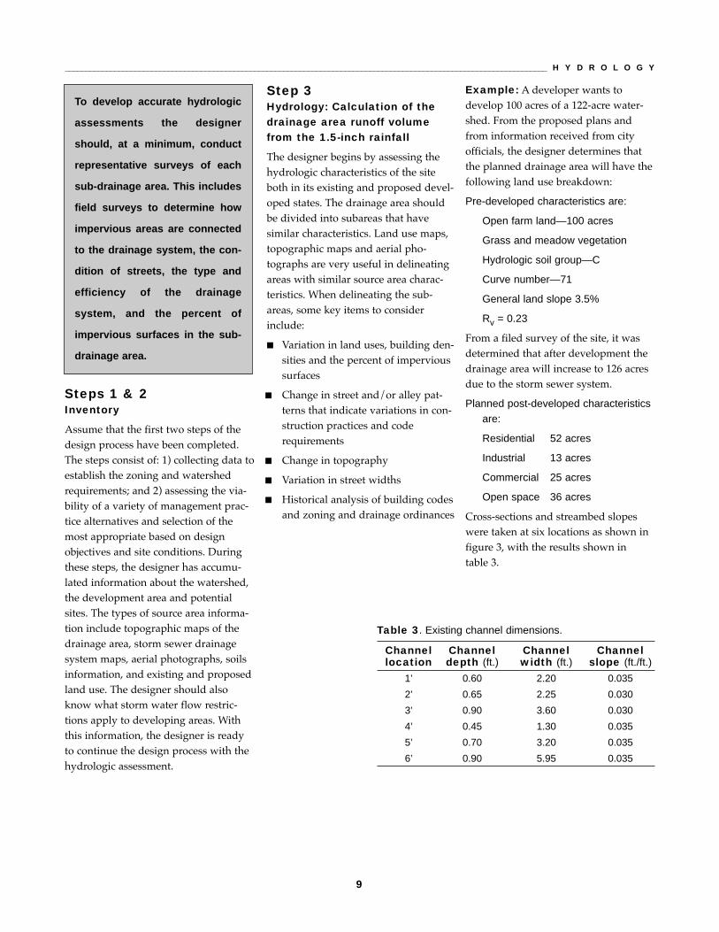
Table 3. Existing channel dimensions.

Channel Channel Channel Channellocation depth (ft.) width (ft.) slope (ft./ft.)

1’ 0.60 2.20 0.035

2’ 0.65 2.25 0.030

3’ 0.90 3.60 0.030

4’ 0.45 1.30 0.035

5’ 0.70 3.20 0.035

6’ 0.90 5.95 0.035

10


1. Residential Area

2. CommercialArea

3. Industrial Area

4. ResidentialArea

5. ResidentialArea

6. Open SpaceAreaI′

H′

G

E

F

′

FD

′

E

C

′ D

A

B

′

C′ B′A′

A′

Legend

A

6

4

5

3

2

1

Flow path location

Flow path designation, existing

Flow path designation, developed

Channel cross sections

Watershed boundary

Intermittent stream

Sub-basin boundaries

Open space

Figure 3. Plan view of the watershed post-development.

11

_____________________________________________________________________________________________________________________ H Y D R O L O G Y

Using data from soil surveys and fielddata the designer assigns an NRCScurve number of 71.

With the collected information andknowing the commonly used develop-ment practices, the designer divides thedeveloped drainage area into six sub-drainage areas as shown in figure 3. Abrief summary of the predominant landuse in each sub-drainage area is sum-marized in table 4.

Area 1. 30.1 acres of low density resi-dential, 4.3 acres of open space�undeveloped on the outside edge,and 1.7 acres of park near thechannel. Total area equals 36.1 acres.(Note: Due to the storm sewersystem, 2.8 acres are added to theexisting drainage area in this sub-watershed area.)

Area 2. 25.0 acres commercial, 6.6acres of open space�undevelopedon the outside edge, and 1.9 acres ofpark near the channel. Total areaequals 33.5 acres.

Area 3. 13.0 acres industrial, 2.3 acresopen space�undeveloped on theoutside edge, and 0.8 acres parknear the channel. Total area equals16.1 acres.

Area 4. 8.2 acres low density residen-tial, 0.4 acres open space�undevel-oped on the outside edge, and 1.4acres of park near the channel. Totalarea equals 10.0 acres (Note: Due tothe storm sewer system, 0.8 acresare added to the existing drainagearea in this sub-basin area.)

Area 5. 13.7 acres low density residen-tial, 3.3 acres of open space on theoutside edge, and 4.2 acres of parknear the channel. Total area equals21.2 acres.

Area 6. 9.1 acres open space�undeveloped.

These sub-drainage areas, groupedaccording to land uses, have source areacharacteristics, the corresponding runoffcoefficients, and runoff volumes for the1.5-inch rainfall shown in table 5.

Table 4. Basin drainage areas.

Sub- Existing Open Open Total area Changesbasin undeveloped Developed area on area near after in drainage

area area outside edge channel development area(acres) (acres) (acres) (acres) (acres) (acres)

res.1 33.3 30.1 4.3 1.7 36.1 +2.8

com.2 33.5 25.0 6.6 1.9 33.5 0.0

ind. 3 16.1 13.0 2.3 0.8 16.1 0.0

res. 4 9.2 8.2 0.4 1.4 10.0 +0.8

res. 5 21.2 13.7 3.3 4.2 21.2 0.0

6 9.1 - - 9.1 9.1 0.0

Total 122.40 90.00 16.90 10.10 126.0 +3.60

12


Table 5 : Calculation of runoff volumes for the developed area.

Area 1 � Residential (36.1 acres)Runoff vol.=

Runoff Product 1.5in. x Rv x (1ft/12in)Source area Area in coefficient of Rv 43,560 sq.ft./ac.characteristic acres Rv x acres x area (in cu. ft.)

Flat roofs—connected 0.01 0.88 0.009 48

Flat roofs—disconnected 0.08 0.23 0.018 100

Pitched roofs—connected 0.41 0.98 0.402 2,191

Pitched Roofs—disconnected 2.85 0.23 0.656 3,572

Paved parking—connected 0.06 0.94 0.056 305

Driveways—connected 0.57 0.94 0.536 2,919

Driveways—disconnected 0.85 0.23 0.196 1,067

Sidewalks—connected 0.33 0.94 0.310 1,690

Sidewalks—disconnected 0.45 0.23 0.104 566

Street area—smooth 1.20 0.84 1.008 5,489

Street area—surface—intermediate 2.86 0.79 2.259 12,301

Large landscape 8.73 0.23 2.008 10,934

Small landscape 16.74 0.23 3.850 20,965

Other pervious areas 0.96 0.23 0.221 1,202

Total 36.10 ——— 11.633 63,349

Rv = 11.633/36.10 = 0.32

Area 2�Commercial (33.5 acres)Runoff vol.=

Runoff Product 1.5 in. x Rv x (1ft/12in)Source area Area in coefficient of Rv 43,560 sq.ft./ac.characteristic acres Rv x acres x area (in cu. ft.)

Flat roofs—connected 4.14 0.88 3.643 19,837

Flat roofs—disconnected 0.93 0.23 0.214 1,167

Paved parking—connected 7.83 0.94 7.360 40,076

Paved parking—disconnected 3.35 0.23 0.771 4,203

Sidewalks—connected 0.28 0.94 0.263 1,433



Large landscape 8.50 .23 1.955 10,663

Small landscape 0.43 .23 0.099 539

Total 33.50 ——— 20.822 113,412

Commercial = 20.82/33.50 = 0.62

13

_____________________________________________________________________________________________________________________ H Y D R O L O G Y

Area 3—Industrial (16.1 acres)

Runoff vol.=Runoff Product 1.5 in. x Rv x (1ft/12in)

Source area Area in coefficient of Rv 43,560 sq.ft./ac.characteristic acres Rv x acres x area (in cu. ft.)

Flat roofs—connected 1.57 0.88 1.382 7,523

Flat roofs—disconnected 2.65 0.23 0.610 3,324

Paved parking—connected 1.10 0.94 1.034 5,630

Paved parking—disconnected 2.51 0.23 0.577 3,149

Unpaved parking—disconnected 0.56 0.23 0.129 703

Driveways—connected 0.10 0.94 0.094 512

Driveways—disconnected 0.15 0.23 0.035 188

Sidewalks—connected 0.02 0.94 0.019 102




Large landscape 5.02 0.23 1.155 6,298

Small landscape 0.12 0.23 0.028 151

Rail areas (other) 0.21 0.23 0.048 263

Total 16.10 ——-.— 6.787 36,969

Rv for industrial = 6.79/16.10 = 0.43

Area 4— Residential (10.0 acres)






Pitched roofs—disconnected 0.62 0.23 0.143 780








Large landscape 2.53 0.23 0.582 3,171

Small landscape 4.56 0.23 1.049 5,711

Other pervious areas 0.20 0.23 0.046 253

Total 10.00 ——-.— 3.392 18,479

Rv = 3.39/10 = 0.34

14


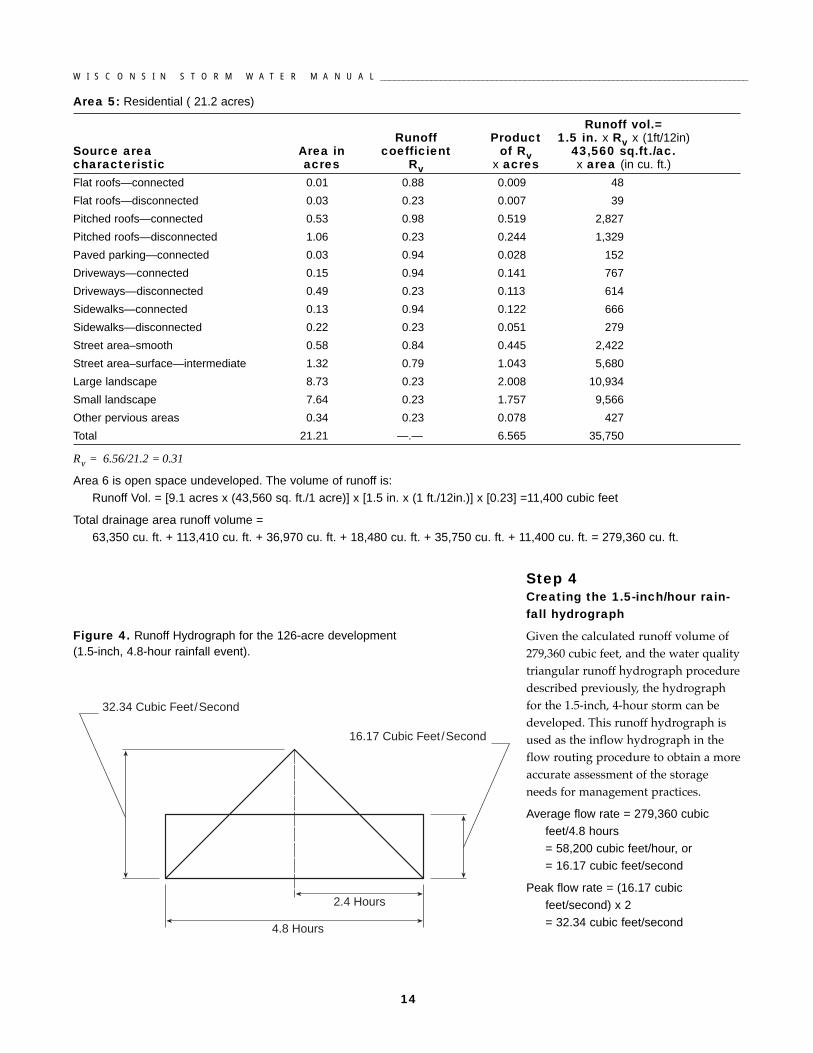
Step 4Creating the 1.5-inch/hour rain-fall hydrograph

Given the calculated runoff volume of279,360 cubic feet, and the water qualitytriangular runoff hydrograph proceduredescribed previously, the hydrographfor the 1.5-inch, 4-hour storm can bedeveloped. This runoff hydrograph isused as the inflow hydrograph in theflow routing procedure to obtain a moreaccurate assessment of the storageneeds for management practices.

Average flow rate = 279,360 cubicfeet/4.8 hours= 58,200 cubic feet/hour, or= 16.17 cubic feet/second

Peak flow rate = (16.17 cubicfeet/second) x 2= 32.34 cubic feet/second

Area 5: Residential ( 21.2 acres)






Pitched roofs—disconnected 1.06 0.23 0.244 1,329






Street area–smooth 0.58 0.84 0.445 2,422

Street area–surface—intermediate 1.32 0.79 1.043 5,680

Large landscape 8.73 0.23 2.008 10,934

Small landscape 7.64 0.23 1.757 9,566

Other pervious areas 0.34 0.23 0.078 427

Total 21.21 —.— 6.565 35,750

Rv = 6.56/21.2 = 0.31

Area 6 is open space undeveloped. The volume of runoff is: Runoff Vol. = [9.1 acres x (43,560 sq. ft./1 acre)] x [1.5 in. x (1 ft./12in.)] x [0.23] =11,400 cubic feet

Total drainage area runoff volume = 63,350 cu. ft. + 113,410 cu. ft. + 36,970 cu. ft. + 18,480 cu. ft. + 35,750 cu. ft. + 11,400 cu. ft. = 279,360 cu. ft.

2.4 Hours

4.8 Hours

32.34 Cubic Feet/Second

16.17 Cubic Feet/Second

Figure 4. Runoff Hydrograph for the 126-acre development (1.5-inch, 4.8-hour rainfall event).

15

_____________________________________________________________________________________________________________________ H Y D R O L O G Y

Step 5Selection of the water qualitymanagement practice

Using the information obtained in steps1 through 4 and information from siteand/or watershed maps, the designer isable to determine potential practicesand possible site locations.

For this example, assume that prelimi-nary data indicate a site in the southernportion of the drainage area that wouldserve the entire drainage area and, inthe designer's judgement, provide thenecessary space to contain the runoff

volume. A detailed site investigationshows that the prevalent soil on the siteis from Hydrologic Soils Group D, withan infiltration rate of less than 0.03inches/ hour, making storage feasible.Space and slope limitations prohibit anartificial wetland stormwater manage-ment system. From these results and thecriteria of the local officials, a detentionbasin is chosen as the most appropriatewater quality practice.

Step 6Develop a preliminary size andrough design for the manage-ment practice

To create a preliminary design, thedesigner follows the appropriate designguidelines of the chosen managementpractice as described in later sections ofthis manual. In this example the guid-ance for detention basins is used todetermine the preliminary design.

From the drainage area survey, a site onthe southern portion of the drainagearea is suitable for a detention basin.The site�s lowest elevation is the bed ofan intermittent stream. The stream isconsidered a non-navigable stream,and, in its existing condition, has flowsonly in the spring and after heavy rains.(See figure 5).

According to detention basin designguidelines, two key considerations arethe permanent pond volume and thesurface area size. The designer nowdetermines the permanent pond surfacearea.

844

846

848

850

852 854

856

858

844

846

848

850

852

854

856

856

858

854

852

850

850

852

854

856

858

860

0 100 200 (ft.)

Figure 5. Detention basin site—existing conditions

16


Calculation of the permanentpond surface area

In most cases the drainage area consistsof mixed land uses. The required pondsurface area is determined by multi-plying the area of the land-use by therecommended drainage area coefficient.An abbreviated table of drainage areacoefficients is found in table 6; a moreextensive table of coefficients may befound in the wet detention basin sectionof this manual.

Table 6. Estimated pond surface area as a percent of the tributarydrainage area

% of drainage

Land use areaCommercial 1.7

Industrial 2.0

Residential 0.8

Open Space 0.6

The recommended pond size as a per-centage of drainage area is calculatedas:

Residential(52 acres x 0.008) = 0.42 acres

Industrial(13 acres x 0.020) = 0.26 acres

Commercial(25 acres x 0.017)= 0.42 acres

Open space(36.0 acres x 0.006) = 0.22 acres

Total = 1.32 acres of surface area for the permanent pond or = 57,500 square feet

The excavation must be sufficient toachieve the necessary surface area of57,500 square feet. With a general slopeof 2 percent, the surface area require-ment appears to plausible with excava-tion of the pond at an elevation of 850feet.

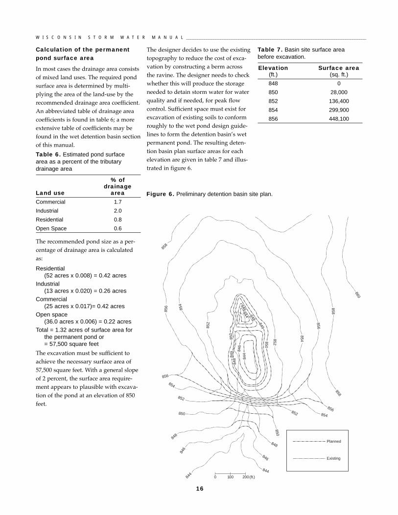
The designer decides to use the existingtopography to reduce the cost of exca-vation by constructing a berm acrossthe ravine. The designer needs to checkwhether this will produce the storageneeded to detain storm water for waterquality and if needed, for peak flowcontrol. Sufficient space must exist forexcavation of existing soils to conformroughly to the wet pond design guide-lines to form the detention basin�s wetpermanent pond. The resulting deten-tion basin plan surface areas for eachelevation are given in table 7 and illus-trated in figure 6.

Table 7. Basin site surface areabefore excavation.

Elevation Surface area(ft.) (sq. ft.)

848 0

850 28,000

852 136,400

854 299,900

856 448,100

844

846

848

850

852 854

856

858

844

846

848

850

852

854

856

856

858

854

852

850

849

848

846

844

844846

848

849850

852

854

856

858

860

Planned

Existing

0 100 200 (ft.)

Figure 6. Preliminary detention basin site plan.

17

_____________________________________________________________________________________________________________________ H Y D R O L O G Y

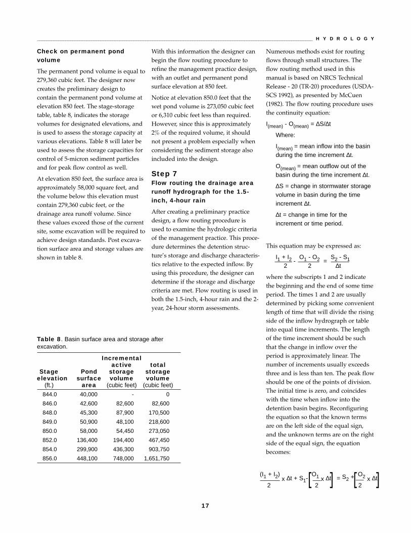
Check on permanent pondvolume

The permanent pond volume is equal to279,360 cubic feet. The designer nowcreates the preliminary design tocontain the permanent pond volume atelevation 850 feet. The stage-storagetable, table 8, indicates the storagevolumes for designated elevations, andis used to assess the storage capacity atvarious elevations. Table 8 will later beused to assess the storage capacities forcontrol of 5-micron sediment particlesand for peak flow control as well.

At elevation 850 feet, the surface area isapproximately 58,000 square feet, andthe volume below this elevation mustcontain 279,360 cubic feet, or thedrainage area runoff volume. Sincethese values exceed those of the currentsite, some excavation will be required toachieve design standards. Post excava-tion surface area and storage values areshown in table 8.

With this information the designer canbegin the flow routing procedure torefine the management practice design,with an outlet and permanent pondsurface elevation at 850 feet.

Notice at elevation 850.0 feet that thewet pond volume is 273,050 cubic feetor 6,310 cubic feet less than required.However, since this is approximately2% of the required volume, it shouldnot present a problem especially whenconsidering the sediment storage alsoincluded into the design.

Step 7Flow routing the drainage arearunoff hydrograph for the 1.5-inch, 4-hour rain

After creating a preliminary practicedesign, a flow routing procedure isused to examine the hydrologic criteriaof the management practice. This proce-dure determines the detention struc-ture�s storage and discharge characteris-tics relative to the expected inflow. Byusing this procedure, the designer candetermine if the storage and dischargecriteria are met. Flow routing is used inboth the 1.5-inch, 4-hour rain and the 2-year, 24-hour storm assessments.

Numerous methods exist for routingflows through small structures. Theflow routing method used in thismanual is based on NRCS TechnicalRelease - 20 (TR-20) procedures (USDA-SCS 1992), as presented by McCuen(1982). The flow routing procedure usesthe continuity equation:

I(mean) - O(mean) = ∆S/∆t

Where:

I(mean) = mean inflow into the basinduring the time increment ∆t.

O(mean) = mean outflow out of thebasin during the time increment ∆t.

∆S = change in stormwater storagevolume in basin during the timeincrement ∆t.

∆t = change in time for the increment or time period.

This equation may be expressed as:

I1 + I2 - O1 - O2 =

S2 - S12 2 ∆t

where the subscripts 1 and 2 indicatethe beginning and the end of some timeperiod. The times 1 and 2 are usuallydetermined by picking some convenientlength of time that will divide the risingside of the inflow hydrograph or tableinto equal time increments. The lengthof the time increment should be suchthat the change in inflow over theperiod is approximately linear. Thenumber of increments usually exceedsthree and is less than ten. The peak flowshould be one of the points of division.The initial time is zero, and coincideswith the time when inflow into thedetention basin begins. Reconfiguringthe equation so that the known termsare on the left side of the equal sign,and the unknown terms are on the rightside of the equal sign, the equationbecomes:

Table 8. Basin surface area and storage after excavation.

Incrementalactive total

Stage Pond storage storageelevation surface volume volume

(ft.) area (cubic feet) (cubic feet)

844.0 40,000 - 0

846.0 42,600 82,600 82,600

848.0 45,300 87,900 170,500

849.0 50,900 48,100 218,600

850.0 58,000 54,450 273,050

852.0 136,400 194,400 467,450

854.0 299,900 436,300 903,750

856.0 448,100 748,000 1,651,750

(I1 + I2) x ∆t + S1-

O1 x ∆t = S2 + O2 x ∆t2 2 2[ [ ]]

18


In this equation, the inflows are takenfrom a hydrograph or table and are,therefore, known. The initial storageand discharge at time zero is usuallyassumed to be zero. This assumes thatthe water is at the lip of the outlet struc-ture and that only the active storagearea will be used in routing. The termsto the right of the equal sign are calcu-lated sequentially from one timesegment to the next, beginning withtime zero. The storage, S2, and outflow,O2, for the current time incrementbecome the storage, S1, and outflow, O2for the next time increment. Thesequence continues until the criticalstorage and discharge characteristics forthe management practice are obtained.

In determining the terms to the right ofthe equal sign, it is necessary to developa number of tables or graphs. To makethis assessment easier, a flow routingprocedure has been devised. An outlineof the process followed by a detaileddescription based upon the 1.5-inch, 4-hour storm follows. An example, as itapplies to detention basin design,accompanies the description. Eachoutlet for a management practice willdiffer in its outlet characteristics and,therefore requires a unique expressionfor the outflow-rating curve. Forexample, the discharge rate for infiltra-tion structures would be the infiltrationrate, while the discharge rate for artifi-cial wetland storm water managementsystems would be the infiltration rate,the evapotranspiration rate and thesurface outflow.

For infiltration facilities and other man-agement practices, the storage volumeneeded to limit the post-developed 2-year, 24-hour peak flow may be beyondthe storage capacity. In this event abypass or flow splitter would then beused to channel flow to a facility thatwould limit the discharge to the 2-year,pre-developed peak flow and store theexcess inflow. The flow routing proce-dure consists of six steps. These steps

are first described and then developedas part of the detention basin designexample.

Step 7-A: Develop an expected inflowhydrograph or table. Determine aconvenient time increment thatdivides the time period of risinginflow into equal time increments.The time segments should bedivided into a minimum of fourtime increments. One of the pointsof division should coincide with thepeak flow time. The initial time iszero, and coincides with the timewhen inflow into the managementpractice begins. In most cases thehydrograph or table will have beendeveloped previously in step 4 ofthe design process. (Note: For the 2-year, 24-hour peak flow assessment,the time segments will follow thetimes identified in the TR-55model.)

Step 7-B: Develop an elevation stage-storage curve or table for the pro-posed site. This is a graphical repre-sentation or tabulation of thestorage volume relative to the waterlevel or stage of the structure. It isnecessary to survey the site anddetermine the surface area associ-ated with a height or elevation inthe structure. The incrementalstorage volume is then determinedby summing the surface areas at thetwo elevations, averaging the areasand multiplying by the change inelevation.

Step 7-C: Develop a stage-dischargecurve or table for the expected dis-charge structure. This is a descrip-tion of the flow discharged from themanagement practice at an associ-ated water surface stage or elevationin the structure.

Step 7-D: Construct a graph or tabledescribing storage, (S1), versus dis-charge, and storage plus discharge,(S2 + [O2/2]∆t), versus discharge.

Step 7-E: Test the outlet and thestorage capacity of the rough designusing the continuity equation, andthe items developed in Steps 7-Athrough 7-D.

Step 7-F: Determine the maximumneeded storage and discharge.Redesign the structure if the waterquality criteria are not satisfied.

The flow routing procedure:an example

Step 7-A. Inflow hydrograph or tabledivided into incremental units oftime.

The drainage area runoff becomes theinflow for the management practice.The time to peak inflow is 2.4 hours. Inthis example, an increment of 28.8minutes was used to give five equalincrements and one increment ending atpeak time of 2.4 hours. Using this timeincrement, table 9 presents the inflowinto the detention basin at the breakpoints.(The determination of the lengthof the time increment is taken fromBarfield, et. al., 1983.)

Table 9. Drainage area runoff for the1.5- inch, 4-hour rainfall.

time inflow rate (min.) (cu. ft./sec.)

0.00 0.00

28.80 6.44

57.60 12.88

86.40 19.32

115.20 25.76

144.00 32.20

172.80 25.76

201.60 19.32

230.40 12.88

259.20 6.44

288.00 0.00

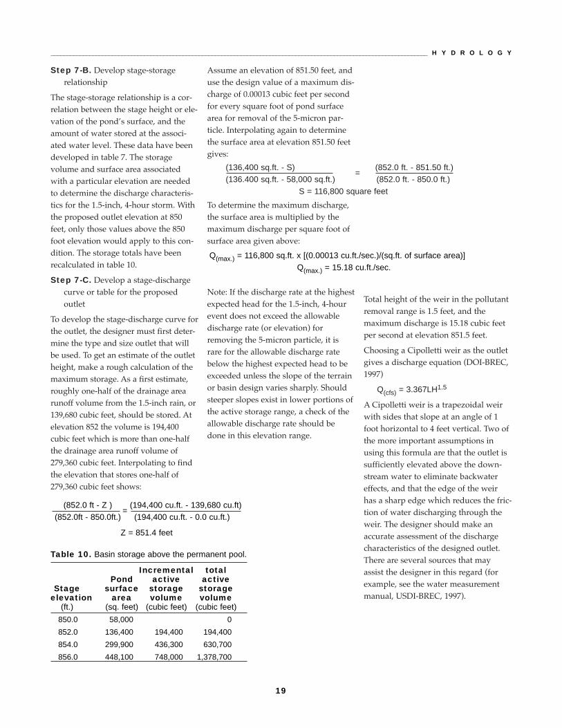
Step 7-B. Develop stage-storage relationship

The stage-storage relationship is a cor-relation between the stage height or ele-vation of the pond�s surface, and theamount of water stored at the associ-ated water level. These data have beendeveloped in table 7. The storagevolume and surface area associatedwith a particular elevation are neededto determine the discharge characteris-tics for the 1.5-inch, 4-hour storm. Withthe proposed outlet elevation at 850feet, only those values above the 850foot elevation would apply to this con-dition. The storage totals have beenrecalculated in table 10.

Step 7-C. Develop a stage-dischargecurve or table for the proposedoutlet

To develop the stage-discharge curve forthe outlet, the designer must first deter-mine the type and size outlet that willbe used. To get an estimate of the outletheight, make a rough calculation of themaximum storage. As a first estimate,roughly one-half of the drainage arearunoff volume from the 1.5-inch rain, or139,680 cubic feet, should be stored. Atelevation 852 the volume is 194,400cubic feet which is more than one-halfthe drainage area runoff volume of279,360 cubic feet. Interpolating to findthe elevation that stores one-half of279,360 cubic feet shows:

Assume an elevation of 851.50 feet, anduse the design value of a maximum dis-charge of 0.00013 cubic feet per secondfor every square foot of pond surfacearea for removal of the 5-micron par-ticle. Interpolating again to determinethe surface area at elevation 851.50 feetgives:

To determine the maximum discharge,the surface area is multiplied by themaximum discharge per square foot ofsurface area given above:

Note: If the discharge rate at the highestexpected head for the 1.5-inch, 4-hourevent does not exceed the allowabledischarge rate (or elevation) forremoving the 5-micron particle, it israre for the allowable discharge ratebelow the highest expected head to beexceeded unless the slope of the terrainor basin design varies sharply. Shouldsteeper slopes exist in lower portions ofthe active storage range, a check of theallowable discharge rate should bedone in this elevation range.

Total height of the weir in the pollutantremoval range is 1.5 feet, and themaximum discharge is 15.18 cubic feetper second at elevation 851.5 feet.

Choosing a Cipolletti weir as the outletgives a discharge equation (DOI-BREC,1997)

Q(cfs) = 3.367LH1.5

A Cipolletti weir is a trapezoidal weirwith sides that slope at an angle of 1foot horizontal to 4 feet vertical. Two ofthe more important assumptions inusing this formula are that the outlet issufficiently elevated above the down-stream water to eliminate backwatereffects, and that the edge of the weirhas a sharp edge which reduces the fric-tion of water discharging through theweir. The designer should make anaccurate assessment of the dischargecharacteristics of the designed outlet.There are several sources that mayassist the designer in this regard (forexample, see the water measurementmanual, USDI-BREC, 1997).

(136,400 sq.ft. - S) =

(852.0 ft. - 851.50 ft.)(136.400 sq.ft. - 58,000 sq.ft.) (852.0 ft. - 850.0 ft.)

S = 116,800 square feet

19

_____________________________________________________________________________________________________________________ H Y D R O L O G Y

Table 10. Basin storage above the permanent pool.

Incremental totalPond active active

Stage surface storage storageelevation area volume volume

(ft.) (sq. feet) (cubic feet) (cubic feet)

850.0 58,000 0

852.0 136,400 194,400 194,400

854.0 299,900 436,300 630,700

856.0 448,100 748,000 1,378,700

(852.0 ft - Z ) =

(194,400 cu.ft. - 139,680 cu.ft)(852.0ft - 850.0ft.) (194,400 cu.ft. - 0.0 cu.ft.)

Z = 851.4 feet

Q(max.) = 116,800 sq.ft. x [(0.00013 cu.ft./sec.)/(sq.ft. of surface area)]Q(max.) = 15.18 cu.ft./sec.

20


Using this formula, a weir width isdetermined by substituting the calcu-lated maximum discharge 15.18 cubicfeet per second for Q(cfs), and 1.5 feetfor H.

15.18 cu.ft. = 3.367 x L x 1.5 ft.1.5

L = 2.45 feet or 29.45 inches wide

Using a 30.00 inch or 2.50 foot weir, theequation becomes:

Q(cfs) = 8.42 H1.5

Table 11 indicates the discharge associ-ated with a given stage height for theproposed weir. The stage height is theheight above the 850.0 feet elevation, orthe surface of the permanent pond.

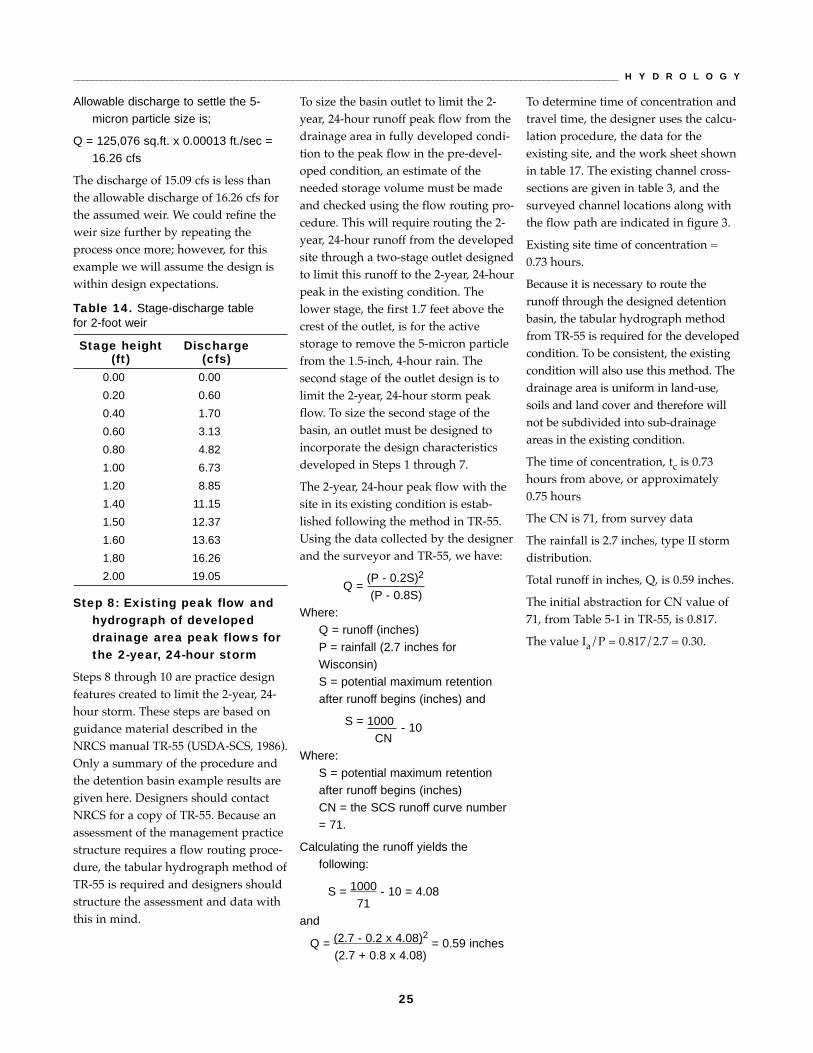
Table 11. Stage-discharge for the 2.5-foot weir.

Stage height (ft.) Discharge (cfs)

0.00 0.00

0.20 0.75

0.40 2.13

0.60 3.91

0.80 6.02

1.00 8.42

1.20 11.07

1.40 13.95

1.50 15.47

1.60 17.04

1.80 20.33

2.00 23.81Table 12. Storage-discharge for 2.5-foot weir.

Surface Disc. * Disc. Vol. for * Storage + Row Elev. Area Storage Rate Increment [(Qave.)(∆ T)]

(ft.) (sq. ft.) (cu. ft.) (cfs) (cu. ft.) (cu. ft.)

1 850.0 58,000 0.0

2 850.20 65,840 12,384 0.75 651 13,035

3 850.40 73,680 26,336 2.13 1,840 28,176

4 850.60 81,520 41,856 3.91 3,381 45,237

5 850.80 89,360 58,944 6.02 5,205 64,149

6 851.00 97,200 77,600 8.42 7,275 84,875

7 851.20 105,040 97,824 11.07 9,563 107,387

8 851.40 112,880 119,616 13.95 12,051 131,667

9 851.60 120,720 142,976 17.04 14,723 157,699

10 851.80 128,560 167,904 20.33 17,568 185,472

11 852.00 136,400 194,400 23.82 20,576 214,976

12 852.20 152,750 223,315 27.48 23,739 247,054

13 852.40 169,100 255,500 31.31 27,048 282,548

14 852.60 185,450 290,955 35.30 30,499 321,454

15 852.80 201,800 329,680 39.45 34,085 363,765

16 853.00 218,150 371,675 43.75 37,801 409,476

17 853.20 234,500 416,940 48.20 41,644 458,584

18 853.40 250,850 465,475 52.79 45,608 511,083

19 853.60 267,200 517,280 57.51 49,691 566,971

20 853.80 283,550 572,355 62.37 53,889 626,244

21 854.00 299,900 630,700 67.36 58,199 688,899

22 854.20 314,720 692,162 72.47 62,618 754,780

23 854.40 329,540 756,588 77.71 67,144 823,732

24 854.60 344,360 823,978 83.07 71,773 895,751

25 854.80 359,180 894,332 88.55 76,505 970,837

26 855.00 374,000 967,650 94.14 81,336 1,048,986

27 855.20 388,820 1,043,932 99.84 86,264 1,130,196

28 855.40 403,640 1,123,178 105.66 91,289 1,214,467

29 855.60 418,460 1,205,388 111.58 96,407 1,301,795

30 855.80 433,280 1,290,562 117.61 101,617 1,392,179

31 856.00 448,100 1,378,700 123.75 106,918 1,485,618

21

_____________________________________________________________________________________________________________________ H Y D R O L O G Y

Step 7-D. Storage versus dischargecurve, and storage plus dischargeversus discharge curve

The storage versus height, and storageplus discharge versus height curve isused to determine the unknown termson the right side of the continuity equa-tion for the flow routing procedure.

Table 12 assists in developing the curveshown in figure 7.

The discharge rate is Q = 8.42 H1.5

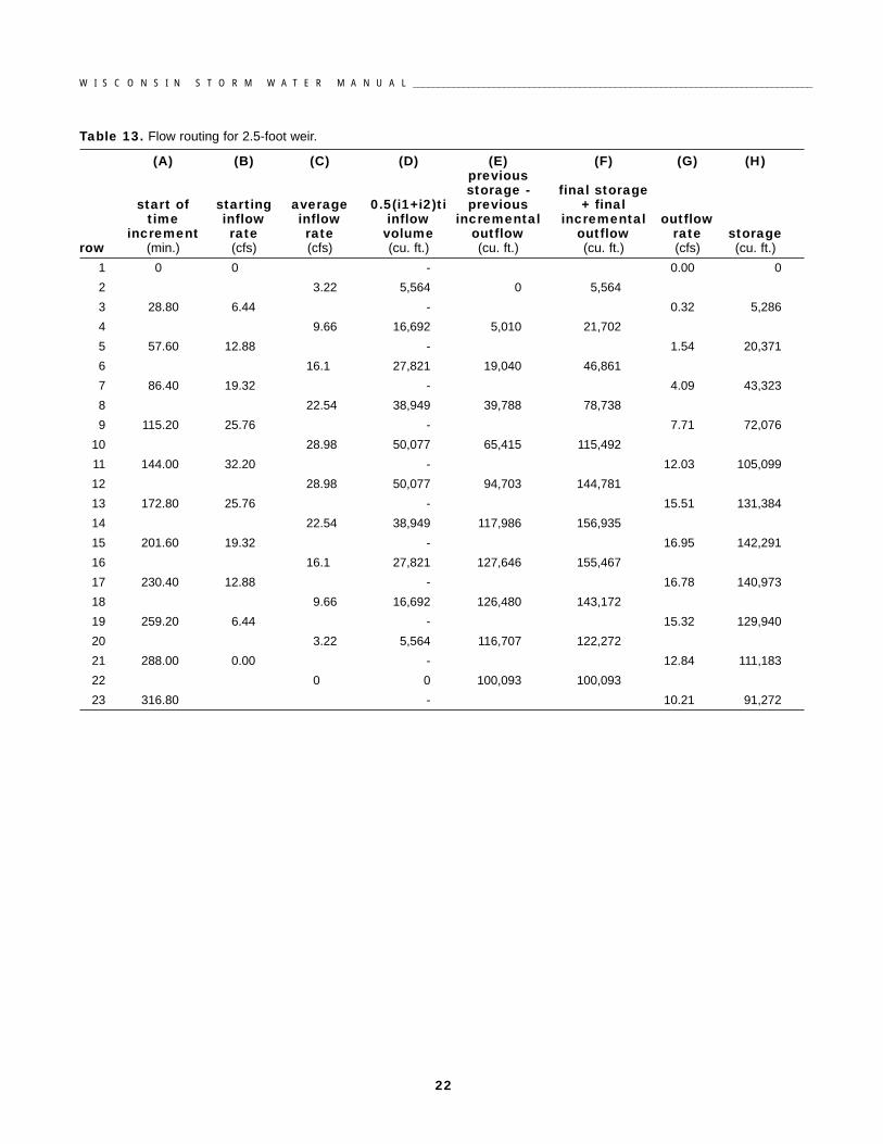
Step 7-E. Construction of the flowrouting table

With the inflow table or hydrograph, andthe storage-discharge curve that havebeen developed, determine the righthand terms of the continuity equation;

A sequential assessment is done takinga known term on the left side of theequation for a series of time incrementsto determine the terms on the right sideof the equation. By taking the beginningand ending inflow rates for each timeincrement from the inflow hydrographor inflow table, averaging them, andmultiplying by the change in time, [(I1 + I2)/2 * ∆t] can be calculated. S1, orstorage at the beginning of the timeincrement, is initially equal to zero, orhas been determined by solving thecontinuity equation for the previoustime increment and is therefore known.Discharge, O1, is initially equal to zeroor determined by solving the continuityequation for the previous time incre-ment and therefore known. The righthand terms are determined by using thestorage-discharge graph or table. Thismethod is usually easier to perform andrecord in a tabular form. The tabularmethod is described and demonstrated

using the actual values for thedetention basin example given intable 13.

Determining the values for the tableinvolves using the drainage area runofffor the 1.5-inch, 4-hour rainfall, table 9,and the storage-discharge graph, figure7 or table 12.

Column A in table 13 represents a spe-cific start and/or finish time for a timeincrement. Values in columns B, G andH represent either a rate of flow orstorage volume for a specific time.These columns have values entered inthose rows with an identified time incolumn A only (in this case, all the odd-numbered rows). Columns C, D, E andF are flow rates and volumes relative tothe entire time increment. Thesecolumns will have values entered inthose rows between times specified incolumn A only (in this case, all the evenrows).

The initial start time, or time zero, is thebeginning of inflow into the manage-ment practice. At the start time, inflow,outflow and storage, columns B, G andH are all assumed to be zero. The timesin column A and the inflow rates incolumn B have been obtained from theinflow table (table 9).

0 50 100 150 200 250 300 350

5

10

15

20

25

30

0

2-3

4

S1

S2 +S2 +O2

2 ∆ t

Storage and Storage + (O2/2)(∆ t), in 1,000s of Cubic Feet

1-

Dis

char

ge, c

fs

Figure 7. Storage-discharge curve.

(I1 + I2) x ∆t + S1 -

O1 x ∆t = S2 + O2 x ∆t

2 2 2[ [] ]

(I1 + I2) x ∆t + S1 -

O1 x ∆t2 2

= S2 + O2 x ∆t2

[ [] ]

22


Table 13. Flow routing for 2.5-foot weir.

(A) (B) (C) (D) (E) (F) (G) (H)previousstorage - final storage

start of starting average 0.5(i1+i2)ti previous + finaltime inflow inflow inflow incremental incremental outflow

increment rate rate volume outflow outflow rate storagerow (min.) (cfs) (cfs) (cu. ft.) (cu. ft.) (cu. ft.) (cfs) (cu. ft.)

1 0 0 - 0.00 0

2 3.22 5,564 0 5,564

3 28.80 6.44 - 0.32 5,286

4 9.66 16,692 5,010 21,702

5 57.60 12.88 - 1.54 20,371

6 16.1 27,821 19,040 46,861

7 86.40 19.32 - 4.09 43,323

8 22.54 38,949 39,788 78,738

9 115.20 25.76 - 7.71 72,076

10 28.98 50,077 65,415 115,492

11 144.00 32.20 - 12.03 105,099

12 28.98 50,077 94,703 144,781

13 172.80 25.76 - 15.51 131,384

14 22.54 38,949 117,986 156,935

15 201.60 19.32 - 16.95 142,291

16 16.1 27,821 127,646 155,467

17 230.40 12.88 - 16.78 140,973

18 9.66 16,692 126,480 143,172

19 259.20 6.44 - 15.32 129,940

20 3.22 5,564 116,707 122,272

21 288.00 0.00 - 12.84 111,183

22 0 0 100,093 100,093

23 316.80 - 10.21 91,272

23

_____________________________________________________________________________________________________________________ H Y D R O L O G Y

In table 13 the column headings aredefined in this manner:

Column A: Time increment is thestart/finish of the time increment.

Example:In this case the time increment is28.8 minutes, or 1,728 seconds takenfrom table 9 for the inflow rates.

Column B: Inflow into the basin at thebeginning of the time increment.(This is the flow from the drainagearea that the basin serves.) Thesevalues are taken from the inflow(Table 9) or hydrograph .

Example:

From table 9, the inflow rates fortimes 0.0 min. and 28.8 min. are 0.0cfs and 6.44 cfs respectively and theinflow rates for times 115.2 min. and144.0 min. are 25.76 cfs and 32.20 cfsrespectively. These values areentered into their respective times incolumn B of table 13.

Column C: Average inflow rate intothe basin over the time segment isthe average inflow of the time incre-ment, or the left term, (I1 + I2)/2, ofthe continuity equation.

Example:

From table 9, the average inflow ofrows 1 and 3 is:

(6.44 cfs + 0.0 cfs)/2 = 3.22 cfs.

The average inflow of rows 9 and 11 is(25.76 cfs + 32.20 cfs)/2 = 28.98 cfs.

These values are entered into column C.

Column D: Inflow volume for the timeincrement, which is calculated bymultiplying the time increment bythe average inflow.

Example:

Row 2: (3.22 cfs) x [(28.8 min. - 0.0min.) x (60 sec./min.)] = 5,564 cu. ft.

Row 10: (28.98 cfs) x [(144.0 min. -115.2 min.) x (60 sec./min.)] =50,077 cu. ft.

Column E: The [(S1-(O1/2) ∆t] term ofthe continuity equation. The storagevolume, (the storage volume at thebeginning of the time incrementobtained from the adjacent rowabove in column H), minus theaverage discharge for the time incre-ment, (the discharge rate at thebeginning of the time incrementobtained from the adjacent rowabove in column G divided by 2)times the change in time for theincrement. In detention basins,when inflow first begins, the activestorage, or water volume above thecrest of the outlet, and the dischargeare assumed to be zero. Infiltrationstructures would be empty with noactive storage and no discharge. Inartificial wetland storm water man-agement systems, the discharge rateis assumed to be the infiltration rateof the structure at the level wheresurface outflow is zero, and evapo-transpiration is assumed to be zero.

Example:

Row 2; from column H, row 1, theinitial storage above elevation 850feet is zero at time zero. Fromcolumn G, row 1 the discharge isalso zero. We have:

(0.0 cu. ft.) - [(0.0 cfs) x (28.8 min. x60 sec./min.)] = 0.0 cu. ft.

In row 10; (72,076 cu. ft.) - [(7.71cfs/2) x ((144.0 min. - 115.2 min.) x(60 sec./min.))] = 65,415 cu. ft.

Column F: Is the [(S2+(O2/2)∆t] termof the continuity equation. Thisvalue is just the sum of the values incolumns D & E.

Example:

Row 2; (5,564 cu. ft.) + (0 cu. ft.) =5,564 cu. ft.

In row 10; 50,077 cu. ft. + 65,415cu. ft. = 115,492 cu. ft.

Column G: The discharge rate at timeT in column A. To determine thedischarge rate, the previous S2 +(O2/2)∆t term in column F in table13 is used with the Storage-Discharge Curve (Figure 7), orStorage-Discharge Table (Table 12).Find the value for S2 + (O2/2)∆tterm on the X-axis of the Storage-Discharge Curve and move verti-cally until intersecting the graph ofS2 + (O2/2)∆t versus discharge line,and then move left horizontallyuntil intersecting the Y-axis toapproximate the discharge rate. Thisvalue is the flow rate at the end ofthe time increment and is placedone row below the value taken incolumn F.

Using the Storage-Discharge Table(Table 12) in the Storage +( Qaver.) x ∆tcolumn, find a value greater and lessthan the value of column F in the FlowRouting Table (table 13). Using thesevalues, the corresponding values fromthe discharge rate column in theStorage-Discharge Table, and the valueof column F in the Flow Routing Table,interpolate a discharge value.

Example:

Row 3, using the Storage-DischargeCurve (Figure 7). The value of 5,564cu. ft.is taken from row 2, column F.Locating this value on the X-axismoving vertically, intersecting the S2+ (O2/2)∆t versus discharge lineand then moving horizontally to theleft, the approximate discharge rateis 0.32 cfs.

Row 11: Repeating the above sequence,from row 10, column F, S2 + (O2/2)∆t =115,492 cu. ft. and the associated dis-charge is approximately 12.03 cfs.

24


Row 3 Storage-Discharge Table. Incolumn F, values 13,035 cu. ft. and 0 arevalues that contain 5,564 cu. ft. the cor-responding values for discharge are 0.75cfs and 0.00 cfs. Interpolating we have:

Repeating this sequence for row 11: O2 = 12.03 cfs

Column H: The storage at time T indi-cated in column B. The storage isdetermined using the Storage-Discharge Curve and the dischargevalue from column G. Using the dis-charge value just determined incolumn G, move horizontally to theright until intersecting the storagecurve, S1. Move vertically down thegraph until intersecting the X-axis todetermine the approximate storagevalue.

This value can also be found using theStorage-Discharge Table (table 12).Again in the Storage + ( Oaver) x ∆tcolumn, find a value greater and lessthan the value of column F in the FlowRouting (table 13). Using these values,the corresponding values from thestorage column in the Storage-Discharge Table, and the value ofcolumn F in the Flow Routing Tableinterpolate a discharge value.

Example:

Row 3, using the Storage-DischargeCurve from column G, we have 0.32 cfs.Locating 0.32 cfs on the Y-axis of theStage-Discharge Curve, move horizon-tally to the right until intersecting the S1discharge curve and then move verti-cally down, we have an estimated valueof 5,300 cu. ft. which we enter into thecolumn H.

Row 11, using the Storage-DischargeCurve; Repeating the above procedure,from column G, discharge = 12.03 cfs,gives an approximate value of 105,000cu. ft. of storage.

Row 3, using the Storage-DischargeTable; Values 13,035 cu. ft. and 0 arevalues that contain 5,564 cu. ft. The cor-responding values for storage fromtable 15 are 12,384 cu. ft and 0.00 cu. ft.Interpolating, we have:

Please note that O2 and S2 now becomeO1 and S1 for the next time increment.

Step 7-F. Maximum necessary storageand discharge

From the Flow Routing Table (table 13)the maximum peak storage and flowoccurs in line 15. The peak storage isapproximately 142,291 cubic feet and themaximum outflow for the outlet is 16.95cubic feet per second. From this pointforward the storage volume and dis-charge rate decline. The predictedmaximum storage volume was 139,690cubic feet, and the maximum allowabledischarge is 15.2 cfs at an elevation of852.5 feet. The actual results are abovethe expected elevation and volume.Checking to determine if the pond willstill settle the 5-micron particle we have:

Required elevation, Er: (values takenfrom table 12)

[(851.6 ft. - Er)/(851.6 ft.- 851.4 ft.)] =[(142,976 cu. ft. - 142,291 cu. ft.)/(142,976 cu.ft. - 119,616 cu. ft.)]

851.6 ft. - Er = 0.2 ft. x 0.0293

Er = 851.6 ft. - 0.0059 ft. = 851.594 ft.

The surface area, A, at this elevation is:(values taken from table 12)

851.59 ft. is approximately 851.6 ft. andthe surface area at this elevation is120,720 sq. ft. allowable discharge, Q, = 120,720 sq. ft. * 0.00013 ft./sec.

Q = 15.69 cfs. (this is less than 16.95 cfs)

The outlet must be reduced to fulfill therequirements of settling velocity for the5-micron particle. We now must returnto step 7-C and choose an outlet sizeand develop a �stage-discharge tableand curve.�

By downsizing the weir, the storageheight is likely to be higher due to therestriction of flow at lower elevations,so use an elevation of 851.8 ft.

Q = 128,560 sq.ft. x 0.00013 ft./sec = 16.71 cfs

Q = 16.71 cfs = 3.367LH1.5

16.71 cfs = 3.367 x L x (1.8’)1.5

L = 2.06 ft. try 2.00 ft. weir

We now must work through theprocess, starting with the developmentof the stage-discharge table (Step 7-B inthis example), storage-discharge tableand curve, and, finally, checking theBMP design by developing a flowrouting table (Step 7-E in this example)as we did earlier. The result of repeatingthese steps is shown in tables 14, 15 and16. The results are, from table 16, line17, a discharge of 15.09 cfs and storageof 156,827 cu.ft. Calculating the corre-sponding elevation and surface area wehave:

E = 851.80 ft. -[(851.80 ft. - 851.60 ft.) x((167,904 cu.ft. - 156,827 cu.ft.)/(167,904 cu.ft. - 142,976 cu.ft.))]

E = 851.7 ft.

A = 128,560 sq.ft. - [(128,560 sq.ft. - 120,720 sq.ft.) x ((167,904 cu.ft. -156,827 cu.ft.)/(167,904 cu.ft. -142,976 cu.ft.))]

A = 125,076 sq.ft.

0.75 cfs - O2 =13,035 cu. ft. - 5,564 cu.ft.

0.75 cfs - 0.00 cfs 13,035 cu ft. - 0.00 cu.ft.

O2 = 0.32 cfs. which is placed in row 3 column G

12,384 cu.ft - S2 =13,035 cu.ft. - 5.564 cu.ft

12,384 cu.ft. - 0.00 cu.ft. 13,035 cu.ft. - 0.00 cu.ftS2 = 5,286 cu. ft.

25

_____________________________________________________________________________________________________________________ H Y D R O L O G Y

Allowable discharge to settle the 5-micron particle size is;

Q = 125,076 sq.ft. x 0.00013 ft./sec =16.26 cfs

The discharge of 15.09 cfs is less thanthe allowable discharge of 16.26 cfs forthe assumed weir. We could refine theweir size further by repeating theprocess once more; however, for thisexample we will assume the design iswithin design expectations.

Table 14. Stage-discharge table for 2-foot weir

Stage height Discharge(ft) (cfs)

0.00 0.00

0.20 0.60

0.40 1.70

0.60 3.13

0.80 4.82

1.00 6.73

1.20 8.85

1.40 11.15

1.50 12.37

1.60 13.63

1.80 16.26

2.00 19.05

Step 8: Existing peak flow andhydrograph of developeddrainage area peak flows forthe 2-year, 24-hour storm

Steps 8 through 10 are practice designfeatures created to limit the 2-year, 24-hour storm. These steps are based onguidance material described in theNRCS manual TR-55 (USDA-SCS, 1986).Only a summary of the procedure andthe detention basin example results aregiven here. Designers should contactNRCS for a copy of TR-55. Because anassessment of the management practicestructure requires a flow routing proce-dure, the tabular hydrograph method ofTR-55 is required and designers shouldstructure the assessment and data withthis in mind.

To size the basin outlet to limit the 2-year, 24-hour runoff peak flow from thedrainage area in fully developed condi-tion to the peak flow in the pre-devel-oped condition, an estimate of theneeded storage volume must be madeand checked using the flow routing pro-cedure. This will require routing the 2-year, 24-hour runoff from the developedsite through a two-stage outlet designedto limit this runoff to the 2-year, 24-hourpeak in the existing condition. Thelower stage, the first 1.7 feet above thecrest of the outlet, is for the activestorage to remove the 5-micron particlefrom the 1.5-inch, 4-hour rain. Thesecond stage of the outlet design is tolimit the 2-year, 24-hour storm peakflow. To size the second stage of thebasin, an outlet must be designed toincorporate the design characteristicsdeveloped in Steps 1 through 7.

The 2-year, 24-hour peak flow with thesite in its existing condition is estab-lished following the method in TR-55.Using the data collected by the designerand the surveyor and TR-55, we have:

Q =(P - 0.2S)2

(P - 0.8S)Where:

Q = runoff (inches)P = rainfall (2.7 inches forWisconsin)S = potential maximum retentionafter runoff begins (inches) and

S = 1000 - 10CN

Where: S = potential maximum retentionafter runoff begins (inches)CN = the SCS runoff curve number= 71.

Calculating the runoff yields thefollowing:

S = 1000 - 10 = 4.0871

and

Q = (2.7 - 0.2 x 4.08)2 = 0.59 inches(2.7 + 0.8 x 4.08)

To determine time of concentration andtravel time, the designer uses the calcu-lation procedure, the data for theexisting site, and the work sheet shownin table 17. The existing channel cross-sections are given in table 3, and thesurveyed channel locations along withthe flow path are indicated in figure 3.

Existing site time of concentration =0.73 hours.

Because it is necessary to route therunoff through the designed detentionbasin, the tabular hydrograph methodfrom TR-55 is required for the developedcondition. To be consistent, the existingcondition will also use this method. Thedrainage area is uniform in land-use,soils and land cover and therefore willnot be subdivided into sub-drainageareas in the existing condition.

The time of concentration, tc is 0.73hours from above, or approximately0.75 hours

The CN is 71, from survey data

The rainfall is 2.7 inches, type II stormdistribution.

Total runoff in inches, Q, is 0.59 inches.

The initial abstraction for CN value of71, from Table 5-1 in TR-55, is 0.817.

The value Ia/P = 0.817/2.7 = 0.30.

26


Using these results, the designer selectsthe peak tabular unit discharge of 348csm/in from page 6 of Exhibit 5-II inTR-55. Using this value the designercalculates a peak flow using the equa-tion on page 5-2 of the TR-55 manual,which is:

q = qt(Am)(Q)

Where: q = hydrograph coordinate (cfs)at hydrograph time t; peak flow isthe only point of concern for theexisting condition.

qt = tabular hydrograph unit dis-charge from exhibit 5 in cubic feetper second for each square per inchof runoff, (csm/in)

Am =drainage area in square miles

Q =depth of runoff in inches

q = (348csm/in)[122.4 acres x (1 sq. mi./640 acres)] [0.59 inches]= 39.3 cfs

Table 15. Stage-discharge table for 2-foot weir.

Surface Disc. Disc. Vol. for StorageRow Elev. Area Storage Rate Increment [(Qave.)(∆ T)]

(ft.) (sq. ft.) (cu. ft.) (cfs) (cu. ft.) (cu. ft.)

1 850.0 58,000 0. 0.0 0. 0.

2 850.20 65,840 12,384 0.60 520 12,904

3 850.40 73,680 26,336 1.70 1,472 27,808

4 850.60 81,520 41,856 3.13 2,704 44,560

5 850.80 89,360 58,944 4.82 4,163 63,107

6 851.00 97,200 77,600 6.73 5,818 83,418

7 851.20 105,040 97,824 8.85 7,648 105,472

8 851.40 112,880 119,616 11.15 9,638 129,254

9 851.60 120,720 142,976 13.63 11,775 154,751

10 851.80 128,560 167,904 16.26 14,051 181,955

11 852.00 136,400 194,400 19.05 16,456 210,856

12 852.20 152,750 223,315 21.97 18,985 242,300

13 852.40 169,100 255,500 25.04 21,632 277,132

14 852.60 185,450 290,955 28.23 24,392 315,347

15 852.80 201,800 329,680 31.55 27,260 356,940

16 853.00 218,150 371,675 34.99 30,232 401,907

17 853.20 234,500 416,940 38.55 33,305 450,245

18 853.40 250,850 465,475 42.22 36,476 501,951

19 853.60 267,200 517,280 46.00 39,741 557,021

20 853.80 283,550 572,355 49.88 43,099 615,454

21 854.00 299,900 630,700 53.87 46,545 677,245

22 854.20 314,720 692,162 57.96 50,080 742,242

23 854.40 329,540 756,588 62.15 53,699 810,287

24 854.60 344,360 823,978 66.44 57,402 881,380

25 854.80 359,180 894,332 70.82 61,186 955,518

26 855.00 374,000 967,650 75.29 65,049 1,032,699

27 855.20 388,820 1,043,932 79.85 68,991 1,112,923

28 855.40 403,640 1,123,178 84.50 73,009 1,196,187

29 855.60 418,460 1,205,388 89.24 77,103 1,282,491

30 855.80 433,280 1,290,562 94.06 81,270 1,371,832

31 856.00 448,100 1,378,700 98.97 85,509 1,464,209

27

_____________________________________________________________________________________________________________________ H Y D R O L O G Y

Table 16. Flow routing table for 2-foot weir.



increment rate rate volume outflow outflow rate storagerow (min.) (cfs) (cfs) (cu. ft.) (cu. ft.) (cu. ft.) (cfs) (cu. ft.)

1 0 0 - 0.00 0

2 3.22 5,564 0 5,564

3 28.80 6.44 - 0.26 5,340

4 9.66 16,692 5,116 21,809

5 57.60 12.88 - 1.26 20,720

6 16.1 27,821 19,634 47,455

7 86.40 19.32 - 3.39 44,523

8 22.54 38,949 41,591 80,540

9 115.20 25.76 - 6.46 74,956

10 28.98 50,077 69,375 119,453

11 144.00 32.20 - 10.20 110,635

12 28.98 50,077 101,820 151,898

13 172.80 25.76 - 13.35 140,362

14 22.54 38,949 128,825 167,775

15 201.60 19.32 - 14.89 154,910

16 16.1 27,821 142,046 169,867

17 230.40 12.88 - 15.09 156,827

18 9.66 16,692 143,788 160,481

19 259.20 6.44 - 14.18 148,226

20 3.22 5,564 135,971 141,535

21 288.00 0.00 - 12.34 130,868

22 0 0 120,202 120,202

23 316.80 - 10.27 111,322

24 0 0 102,445 102,445

25 345.60 - 8.56 95,048

26 0 0 87,653 87,653

27 374.40 - 7.14 81,483

28 0 0 75,317 75,317

29 403.20 - 5.97 70,159

30 0 0 65,003 65,003

31 432.00 - 5.00 60,685

32 0 0 56,367 56,367

33 460.80 4.21 52,734

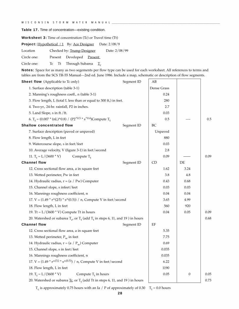
28


Table 17. Time of concentration—existing condition.

Worksheet 3: Time of concentration (Tc) or Travel time (Tt)

Project: Hypothetical # 1 By: Ace Designer Date: 2/08/9

Location Checked by: Trump Designer Date: 2/08/99

Circle one: Present Developed Present

Circle one: Tc Tt Through Subarea Tc

Notes: Space for as many as two segements per flow type can be used for each worksheet. All references to terms andtables are from the SCS TR-55 Manual�2nd ed. June 1986. Include a map, schematic or description of flow segments.

Sheet flow (Applicable to Tc only) Segment ID AB

1. Surface description (table 3-1) Dense Grass

2. Manning�s roughness coeff., n (table 3-1) 0.24

3. Flow length, L (total L less than or equal to 300 ft,) in feet. 280

4. Two-yr., 24-hr. rainfall, P2 in inches. 2.7

5. Land Slope, s in ft./ft. 0.03

6. Tt = (0.007 * (nL)^0.8) / (P2^0.5 * s^0.4)Compute Tt 0.5 �- 0.5

Shallow concentrated flow Segment ID BC

7. Surface description (paved or unpaved) Unpaved

8. Flow length, L in feet 880

9. Watercourse slope, s in feet/feet 0.03

10. Average velocity, V (figure 3-1) in feet/second 2.8

11. Tt = L/(3600 * V) Compute Tt 0.09 �� 0.09

Channel flow Segment ID CD DE

12. Cross sectional flow area, a in square feet 1.62 3.24

13. Wetted perimeter, Pw in feet 3.8 4.8

14. Hydraulic radius, r = (a / Pw) Computer 0.43 0.68

15. Channel slope, s infeet/feet 0.03 0.03

16. Mannings roughness coefficient, n 0.04 0.04

17. V = (1.49 * r^(2Ú3) * s^(0.5)) / n, Compute V in feet/second 3.65 4.99

18. Flow length, L in feet 560 920

19. Tt = L/(3600 * V) Compute Tt in hours 0.04 0.05 0.09

20. Watershed or subarea Tc, or Tt (add Tt in steps 6, 11, and 19 ) in hours 0.68

Channel flow Segment ID EF

12. Cross sectional flow area, a in square feet 5.35

13. Wetted perimeter, Pw in feet 7.75

14. Hydraulic radius, r = (a / Pw) Computer 0.69

15. Channel slope, s in feet/feet 0.035

16. Mannings roughness coefficient, n 0.035

17. V = (1.49 * r^(2Ú3) * s^(0.5)) / n, Compute V in feet/second 6.22


19. Tt = L/(3600 * V) Compute Tt in hours 0.05 0 0.05

20. Watershed or subarea Tc, or Tt (add Tt in steps 6, 11, and 19 ) in hours 0.73

Tc is approximately 0.75 hours with an Ia / P of approximately of 0.30 Tt = 0.0 hours

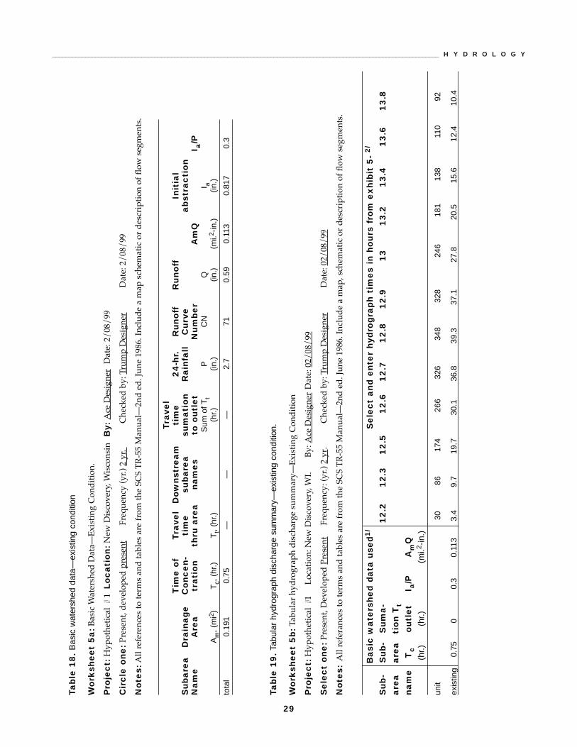
_____________________________________________________________________________________________________________________ H Y D R O L O G Y

Tab

le 1

8.

Bas

ic w

ater

shed

dat

a—ex

istin

g co

nditi

on

Wo

rksh

ee

t 5

a:B

asic

Wat

ersh

ed D

ata —

Exi

stin

g C

ond

itio

n.

Pro

jec

t:H

ypot

heti

cal #

1L

oc

ati

on

:New

Dis

cove

ry, W

isco

nsin

By:

Ace

Des

igne

rD

ate:

2/

08/

99

Cir

cle

on

e:P

rese

nt, d

evel

oped

pr e

sent

Freq

uenc

y (y

r.) 2

yr.

Che

cked

by:

Tru

mp

Des

igne

rD

ate:

2/

08/

99

No

tes:

All

refe

renc

es to

term

s an

d ta

bles

are

fro

m th

e SC

S T

R-5

5 M

anua

l�2n

d e

d. J

une

1986

. Inc

lud

e a

map

sch

emat

ic o

r d

escr

ipti

on o

f fl

ow s

egm

ents

.

Tab

le 1

9.T

abul

ar h

ydro

grap

h di

scha

rge

sum

mar

y—ex

istin

g co

nditi

on.

Wo

rksh

ee

t 5

b:T

abul

ar h

ydro

grap

h d

isch

arge

sum

mar

y —E

xist

ing

Con

dit

ion

Pro

jec

t:H

ypot

heti

cal #

1L

ocat

ion:

New

Dis

cove

ry, W

I. B

y: A

ce D

esig

ner

Dat

e: 0

2/08

/99

Se

lec

t o

ne

:Pre

sent

, Dev

elop

ed P

rese

ntFr

eque

ncy:

(yr

.) 2

yr.

Che

cked

by:

Tru

mp

Des

igne

rD

ate:

02/

08/

99

No

tes:

All

refe

ranc

es to

term

s an

d ta

bles

are

fro

m th

e SC

S T

R-5

5 M

anua

l—2n

d e

d. J

une

1986

. Inc

lud

e a

map

, sch

emat

ic o

r d

escr

ipti

on o

f fl

ow s

egm

ents

.

Tra

vel

Tim

e o

f Tra

vel

Do

wn

stre

am

tim

e2

4-h

r.R

un

off

Ru

no

ffIn

itia

lS

ub

are

aD

rain

ag

eC

on

ce

n-

tim

esu

ba

rea

sum

ati

on

Ra

infa

llC

urv

e

ab

stra

cti

on

Na

me

Are

atr

ati

on

thru

are

an

am

es

to o

utl

et

Nu

mb

er

Am

QI a

/PS

um o

f Tt

PC

NQ

I aA

m,

(mi2

)T

c, (

hr.)

Tt,

(hr.)

(hr.)

(in.)

(in.)

(mi.2

-in.)

(in.)

tota

l0.

191

0.75

——

—2.

771

0.59

0.11

30.

817

0.3

Ba

sic

wa

ters

he

d d

ata

use

d1

/S

ele

ct

an

d e

nte

r h

ydro

gra

ph

tim

es

in h

ou

rs f

rom

ex

hib

it 5

- 2

/

Su

b-

Su

b-

Su

ma

-1

2.2

12

.31

2.5

12

.61

2.7

12

.81

2.9

13

13

.21

3.4

13

.61

3.8

are

aa

rea

tio

n T

tn

am

eT

co

utl

et

I a/P

Am

Q(h

r.)(h

r.)(m

i.2-in

.)

unit

3086

174

266

326

348

328

246

181

138

110

92

exis

ting

0.75

00.

30.

113

3.4

9.7

19.7

30.1

36.8

39.3

37.1

27.8

20.5

15.6

12.4

10.4

29

30


Table 20. Time of concentration worksheet—developed condition.

Worksheet 3: Time of concentration (Tc) or Travel time (Tt)

Project: Hypothetical # 1

Location: Ideal Wisconsin

Designed by: Ace Designer Date: 2/08/99

Checked by: Trump Designer Date: 2/08/99

Circle one: present, developed Circle one: Tc Tt

Notes: Space for as many as two segments per flow type can be used for each worksheet. All references to terms and tablesare from the SCS TR-55 Manual�2nd ed. June 1986. Include a map, schematic or description of flow segments.

Sheet flow (Applicable to Tc only) Segment ID AB

1. Surface description (table 3-1) Dense Grass

2. Manning�s roughness coeff., n (table 3-1) 0.24

3. Flow length, L (total L less than or equal to 300 ft.,) in ft. 115

4. 2-year, 24-hour rainfall, P2 in inches. 2.7

5. Land slope, s in ft./ft. 0.03

6. Tt = (0.007 * (nL)^0.8) / (P2^0.5* s^0.4) Compute T 0.25 0 0.25

Shallow concentrated flow Segment ID BC CD

7. Surface description (paved or unpaved) Unpaved Paved

8. Flow length, L in feet 65 265

9. Watercourse slope, s in feet 0.02 0.03

10. Average velocity, V (figure 3-1) in feet/second 2.2 3.6

11. Tt = L/(3600 * V) Compute Tt 0.01 0.02 0.03

Channel flow Segment ID DE

12. Cross sectional flow area, a, in square feet 0.9

13. Wetted perimeter, Pw in feet 4.2

14. Hydraulic radius, r = (a/Pw), Compute r 0.21

15. Channel slope, s in feet/feet 0.04

16. Mannings roughness coefficient, n 0.02

17. V = (1.49 * (r^2Ú3) * s^(0.5))/n, Compute V in feet/second 4.5


19. Tt = L/(3600 * V) Compute Tt in hours 0.03 0.03

20. Watershed or subarea Tc, or Tt (add Tt in steps 6, 11, and 19) in hours 0.30

Tables 18 an 19 show the calculations ofthe peak flow for the existing condition.To develop the hydrograph for thedrainage area in the fully developedcondition, repeat the TR-55 sequencethat was used to create the 2-year, 24-hour peak flow for the drainage area inits existing condition. Calculate the timeof concentration using figure 5. The flowtimes for this example were calculatedusing both TR-55 and pipe flow calcula-

tion. The Standard Handbook for CivilEngineers�(Merritt, 1983) was used forthe pipe calculations based on theManning equation. Please note that thelongest flow path in the developed con-dition is different than the flow path inthe existing condition, because thedrainage area serviced by the stormsewer system changes the flow direction.

Please refer to tables 20 through 22 for

the results of the flow table in thedeveloped condition. The informationin the tabular hydrograph dischargesummary can be used to produce anoutflow hydrograph and also informsthe designer of the 2-year, 24-hour peakflow, and required maximum storageneeded for the management practicewith the area in the fully developedcondition.

_____________________________________________________________________________________________________________________ H Y D R O L O G Y

31

Tab

le 2

1.B

asin

wat

ersh

ed d

ata—

deve

lope

d co

nditi

on.

Wo

rksh

ee

t 5

a:

Bas

ic w

ater

shed

dat

a�d

evel

oped

con

dit

ion

Proj

ect H

ypot

heti

cal #

1L

ocat

ion

New

Dis

cove

ry, W

isco

nsin

By:

Ace

Des

igne

rD

ate:

2/

08/

99

Cir

cle

one:

Pre

sent

, Dev

elop

ed D

evel

oped

Freq

uenc

y (y

r.) 2

yr.

Che

cked

By:

Tru

mp

Des

igne

rD

ate:

2/

08/

99N

ote

s:A

ll re

fere

nces

to te

rms

and

tabl

es a

re f

rom

the

SCS

TR

-55

Man

ual�

2nd

ed

. Jun

e 19

86. I

nclu

de

a m

ap, s

chem

atic

or

des

crip

tion

of

flow

seg

men

ts.

Tra

vel

Tim

e o

f Tra

vel

Do

wn

stre

am

tim

e2

4-h

r.R

un

off

Ru

no

ffIn

itia

lS

ub

are

aD

rain

ag

eC

on

ce

n-

tim

esu

ba

rea

sum

ati

on

Ra

infa

llC

urv

e

ab

stra

cti

on

Na

me

Are

atr

ati

on

thru

are

an

am

es

to o

utl

et

Nu

mb

er

Am

QI a

/PS

um o

f Tt

PC

NQ

I aA

m,

(mi2

)T

c, (

hr.)

Tt,

(hr.)

(hr.)

(in.)

(in.)

(mi.2

-in.)

(in.)

10.

056

0.3

-2,

5,6

0.09

2.7

80.5

1.06

0.06

00.

484

0.18

20.

052

0.3

0.04

5,6

0.05

2.7

88.2

1.57

0.08

20.

268

0.10

30.

025

0.3

0.03

40.

022.

787

.11.

490.

037

0.29

60.

11

40.

016

0.2

0.02

60

2.7

80.8

1.08

0.01

70.

475

0.18

50.

033

0.3

0.05

-0

2.7

78.8

0.96

0.03

20.

538

0.20

60.

014

0.5

0.00

5-

02.

771

.00.

590.

008

0.81

70.

30

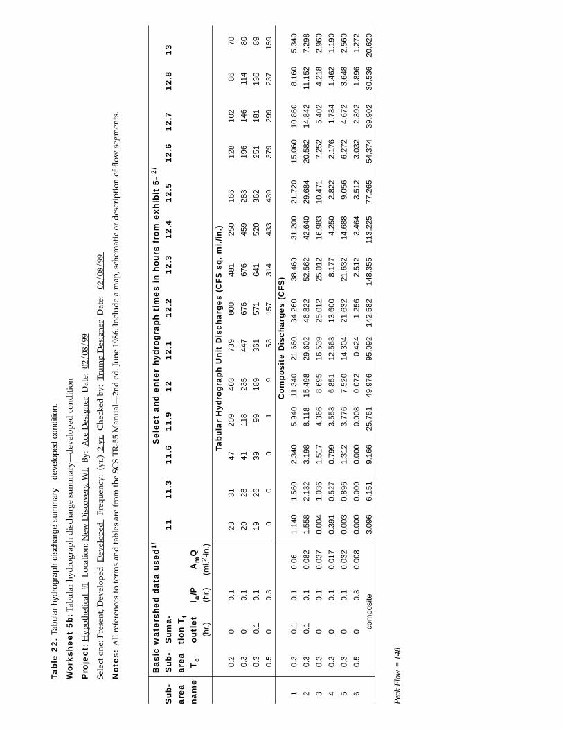
Ba

sic

wa

ters

he

d d

ata

use

d1

/S

ele

ct

an

d e

nte

r h

ydro

gra

ph

tim

es

in h

ou

rs f

rom

ex

hib

it 5

- 2

/

Su

b-

Su

b-

Su

ma

-1

11

1.3

11

.61

1.9

12

12

.11

2.2

12

.31

2.4

12

.51

2.6

12

.71

2.8

13

are

aa

rea

tio

n T

tn

am

eT

co

utl

et

I a/P

Am

Q(h

r.)(h

r.)(m

i.2-in

.)

Tab

ula

r H

ydro

gra

ph

Un

it D

isc

ha

rge

s (C

FS

sq

. m

i./in

.)

0.2

00.

123

3147

209

403

739

800

481

250

166

128

102

8670

0.3

00.

120

2841

118

235

447

676

676

459

283

196

146

114

80

0.3

0.1

0.1

1926

3999

189

361

571

641

520

362

251

181

136

89

0.5

00.

30

00

19

5315

731

443

343

937

929

923

715

9

Co

mp

osi

te D

isc

ha

rge

s (C

FS

)

10.

30.

10.

10.

061.

140

1.56

02.

340

5.94

011

.340

21.6

6034

.260

38.4

6031

.200

21.7

2015

.060

10.8

608.

160

5.34

0

20.

30.

10.

10.

082

1.55

82.

132

3.19

88.

118

15.4

9829

.602

46.8

2252

.562

42.6

4029

.684

20.5

8214

.842

11.1

527.

298

30.

30

0.1

0.03

70.

004

1.03

61.

517

4.36

68.

695

16.5

3925

.012

25.0

1216

.983

10.4

717.

252

5.40

24.

218

2.96

0

40.

20

0.1

0.01

70.

391

0.52

70.

799

3.55

36.

851

12.5

6313

.600

8.17

74.

250

2.82

22.

176

1.73

41.

462

1.19

0

50.

30

0.1

0.03

20.

003

0.89

61.

312

3.77

67.

520

14.3

0421

.632

21.6

3214

.688

9.05

66.

272

4.67

23.

648

2.56

0

60.

50

0.3

0.00

80.

000

0.00

00.

000

0.00

80.

072

0.42

41.

256

2.51

23.

464

3.51

23.

032

2.39

21.

896

1.27

2

com

posi

te3.

096

6.15

19.

166

25.7

6149

.976

95.0

9214

2.58

214

8.35

511

3.22

577

.265

54.3

7439

.902

30.5

3620

.620

Pea

k Fl

ow =

148

Tab

le 2

2.

Tabu

lar

hydr

ogra

ph d

isch

arge

sum

mar

y—de

velo

ped

cond

ition

.

Wo

rksh

ee

t 5

b:T

abul

ar h

ydro

grap

h d

isch

arge

sum

mar

y�d

evel

oped

con

dit

ion

Pro

jec

t:H

ypot

heti

cal #

1L

ocat

ion:

New

Dis

cove

ry, W

I.B

y: A

ce D

esig

ner

Dat

e: 0

2/08

/99

Sele

ct o

ne: P

rese

nt, D

evel

oped

Dev

elop

ed

Freq

uenc

y: (

yr.)

2 y

r.C

heck

ed b

y: T

rum

p D

esig

ner

Dat

e:

02/

08/

99

No

tes:

All

refe

renc

es to

term

s an

d ta

bles

are

fro

m th

e SC

S T

R-5

5 M

anua

l�2n

d e

d. J

une

1986

. Inc

lud

e a

map

, sch

emat

ic o

r d

escr

ipti

on o

f flo

w s

egm

ents

.

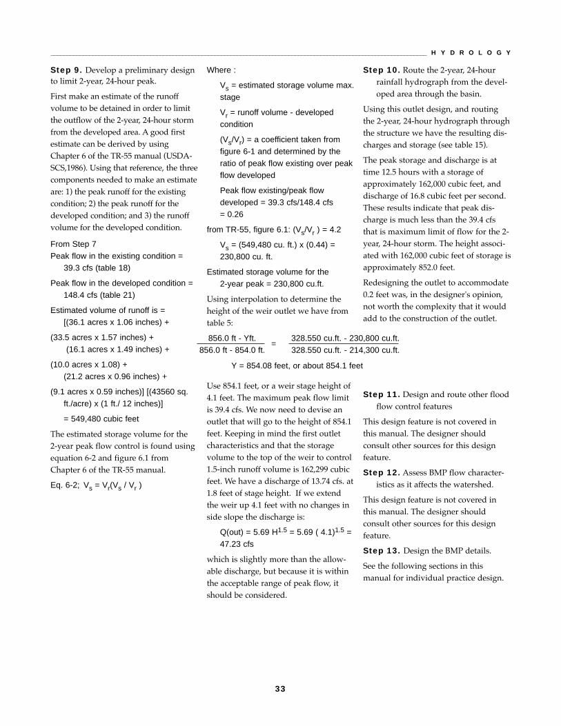
33

_____________________________________________________________________________________________________________________ H Y D R O L O G Y

Step 9. Develop a preliminary designto limit 2-year, 24-hour peak.

First make an estimate of the runoffvolume to be detained in order to limitthe outflow of the 2-year, 24-hour stormfrom the developed area. A good firstestimate can be derived by usingChapter 6 of the TR-55 manual (USDA-SCS,1986). Using that reference, the threecomponents needed to make an estimateare: 1) the peak runoff for the existingcondition; 2) the peak runoff for thedeveloped condition; and 3) the runoffvolume for the developed condition.

From Step 7 Peak flow in the existing condition =

39.3 cfs (table 18)

Peak flow in the developed condition =148.4 cfs (table 21)

Estimated volume of runoff is = [(36.1 acres x 1.06 inches) +

(33.5 acres x 1.57 inches) +(16.1 acres x 1.49 inches) +

(10.0 acres x 1.08) + (21.2 acres x 0.96 inches) +

(9.1 acres x 0.59 inches)] [(43560 sq.ft./acre) x (1 ft./ 12 inches)]

= 549,480 cubic feet

The estimated storage volume for the 2-year peak flow control is found usingequation 6-2 and figure 6.1 fromChapter 6 of the TR-55 manual.

Eq. 6-2; Vs = Vr(Vs / Vr )

Where :

Vs = estimated storage volume max.stage

Vr = runoff volume - developed condition

(Vs/Vr) = a coefficient taken fromfigure 6-1 and determined by theratio of peak flow existing over peakflow developed

Peak flow existing/peak flow developed = 39.3 cfs/148.4 cfs = 0.26

from TR-55, figure 6.1: (Vs/Vr ) = 4.2

Vs = (549,480 cu. ft.) x (0.44) =230,800 cu. ft.

Estimated storage volume for the 2-year peak = 230,800 cu.ft.

Using interpolation to determine theheight of the weir outlet we have fromtable 5:

Use 854.1 feet, or a weir stage height of4.1 feet. The maximum peak flow limitis 39.4 cfs. We now need to devise anoutlet that will go to the height of 854.1feet. Keeping in mind the first outletcharacteristics and that the storagevolume to the top of the weir to control1.5-inch runoff volume is 162,299 cubicfeet. We have a discharge of 13.74 cfs. at1.8 feet of stage height. If we extendthe weir up 4.1 feet with no changes inside slope the discharge is:

Q(out) = 5.69 H1.5 = 5.69 ( 4.1)1.5 =47.23 cfs

which is slightly more than the allow-able discharge, but because it is withinthe acceptable range of peak flow, itshould be considered.

Step 10. Route the 2-year, 24-hourrainfall hydrograph from the devel-oped area through the basin.

Using this outlet design, and routingthe 2-year, 24-hour hydrograph throughthe structure we have the resulting dis-charges and storage (see table 15).

The peak storage and discharge is attime 12.5 hours with a storage ofapproximately 162,000 cubic feet, anddischarge of 16.8 cubic feet per second.These results indicate that peak dis-charge is much less than the 39.4 cfsthat is maximum limit of flow for the 2-year, 24-hour storm. The height associ-ated with 162,000 cubic feet of storage isapproximately 852.0 feet.

Redesigning the outlet to accommodate0.2 feet was, in the designer's opinion,not worth the complexity that it wouldadd to the construction of the outlet.

Step 11. Design and route other floodflow control features

This design feature is not covered inthis manual. The designer shouldconsult other sources for this designfeature.

Step 12. Assess BMP flow character-istics as it affects the watershed.

This design feature is not covered inthis manual. The designer shouldconsult other sources for this designfeature.

Step 13. Design the BMP details.

See the following sections in thismanual for individual practice design.

856.0 ft - Yft. =

328.550 cu.ft. - 230,800 cu.ft.856.0 ft - 854.0 ft. 328.550 cu.ft. - 214,300 cu.ft.

Y = 854.08 feet, or about 854.1 feet

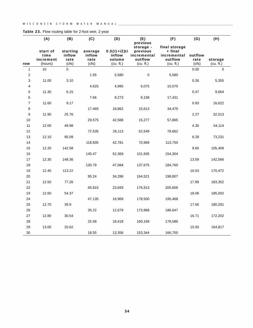
34


Table 23. Flow routing table for 2-foot weir, 2-year



increment rate rate volume outflow outflow rate storagerow (hours) (cfs) (cfs) (cu. ft.) (cu. ft.) (cu. ft.) (cfs) (cu. ft.)

1 10 0 - 0.00 0

2 1.55 5,580 0 5,580

3 11.00 3.10 0.26 5,355

4 4.625 4,995 5,075 10,070

5 11.30 6.15 0.47 9,664

6 7.66 8,273 9,158 17,431

7 11.60 9.17 0.93 16,622

8 17.465 18,862 15,613 34,475

9 11.90 25.76 2.27 32,513

10 29.575 42,588 15,277 57,865

11 12.00 49.98 4.35 54,114

12 72.535 26,113 52,549 78,662

13 12.10 95.09 6.28 73,231

14 118.835 42,781 70,969 113,750

15 12.20 142.58 9.65 105,409

16 145.47 52,369 101,935 154,304

17 12.30 148.36 13.59 142,566

18 130.79 47,084 137,675 184,760

19 12.40 113.22 16.53 170,472

20 95.24 34,286 164,521 198,807

21 12.50 77.26 17.89 183,352

22 65.815 23,693 176,913 200,606

23 12.60 54.37 18.06 185,002

24 47.135 16,969 178,500 195,468

25 12.70 39.9 17.56 180,291

26 35.22 12,679 173,968 186,647

27 12.80 30.54 16.71 172,202

28 25.58 18,418 160,169 178,586

29 13.00 20.62 15.93 164,817

30 18.55 13,356 153,344 166,700

35

_____________________________________________________________________________________________________________________ H Y D R O L O G Y

Summary

The method described here isdevised to calculate the size ofcontrol practice structures to

accomplish an 80% removal of total sus-pended solids on an annual basis andlimit the peak flow from a drainage areato the peak flow in the pre-developedcondition. The method achieves this bycalculating the runoff volume, peak flowand hydrographs for the pre- and post-developed conditions. To simplify theprocedure, it is necessary that conserva-tively sized structures be designed toaccommodate a wide range of site con-ditions.

Designers are encouraged to use theSLAMM computer model and othermodels approved by local governmentsto design structures that are more eco-nomical. All structures must achieve80% removal of the total suspendedsolids on an annual basis, and maintainexiting peak flow levels in receivingwater bodies.

ReferencesBarfield, B. J., R.C. Warner and C. T.

Haan. 1983. Applied Hydrology andSedimentology for Disturbed Areas,Oklahoma Technical Press,Oklahoma.

Bicknell, B.R., J. C. Inhoff, J.L. Kittle Jr.,A.S. Donugian Jr., and R.C. Johnson.1997. Hydrological SimulationProgram�fortran: User�s Manualfor Version 11. US-EPA EPA/600/R-97/080. Athens, GA.

Leopold, L.B. 1968. Hydrology of UrbanLand Planning�A Guidebook onthe Hydrologic Effects of Urbanland Use. USGS Circ. 554.

McCuen, R.H. 1982. A Guide toHydrologic Analysis Using SCSMethods, Prentice-Hall, Inc., NJ.

Merritt, F.S. editor. 1983. StandardHandbook for Civil Engineers,Third Edition, McGraw-Hill BookCo., New York.

Pitt, R. 1989. Source Loading andManagement. An Urban NonpointSource Water Quality Model.Volume 1. Model Development andSummary. Dept. of CivilEngineering. Univ. Of Alabama.Birmingham,. AL.

Pitt, R. 1994. Using the Source Loadingand Management Model (SLAMM)and DETPOND for StormwaterManagement, Department ofEngineering ProfessionalDevelopment, U.W. Extension-Madison.

Prey, J. 1994. The Wisconsin StormwaterManual. Part 1. Overview. WI-DNR.Madion.

USDI-BREC. 1997. Water MeasurementManual, 3rd ed. Departmentof theInterior. Washington, DC.

US-EPA. 1983. Results of theNationwide Urban Runoff Program.Water Planning Division, Vol. 1.NTIS # PB84-185552. Washington, DC.

USDA-SCS. 1986. Urban Hydrology forSmall Watersheds. Tech. Rel. 55.Natural Resources ConservationService. Washington, DC.

USDA-SCS. 1992. Computer Programfor Project Formulation - Hydrology.Tech. Rel. 20. Natural ResourcesConservation Service. Washington, DC.

Walker, W. J., Jr. 1990. P8 UrbanCatchment Model � ProgramDocumentation: Version 1.1.Prepared for IEP, Inc.Northborough, MA.

WI-DNR. 1997. Personal communica-tion. Wisconsin Department ofNatural Resources. Madison.

Wolman, M. G. and A.P. Schick. 1967.Effect of Construction on FluvialSediment: Urban and SuburbanAreas of Maryland. Water resourcesResearch 3:451-462.

Authors: Terry Donovan is a storm water engineer and John Pfender is a watershed planner with the WisconsinDepartment of Natural Resources.

Series editor: Gary Bubenzer is a professor of biological systems engineering and environmental studies with the Collegeof Agricultural and Life Sciences at the University of Wisconsin�Madison.

Issued in furtherance of Cooperative Extension work, Acts of May 8 and June 30, 1914, in cooperation with the U.S.Department of Agriculture, University of Wisconsin�Extension, Cooperative Extension. University of Wisconsin�Extensionprovides equal opportunities in employment and programming, including Title IX and ADA requirements. If you need thisinformation in an alternative format, contact the Office of Equal Opportunity and Diversity Programs or call ExtensionPublishing at (608)262-2655.

©2000 by the Board of Regents of the University of Wisconsin System doing business as the division of CooperativeExtension of the University of Wisconsin�Extension. Send inquiries about copyright permission to Director, CooperativeExtension Publishing, 201 Hiram Smith Hall, 1545 Observatory Dr., Madison, WI 53706.

Partial funding for this publication was provided by the Wisconsin Department of Natural Resources.

You can obtain copies of this publication from your Wisconsin county Extension office or from Cooperative ExtensionPublications, Room 170, 630 W. Mifflin Street, Madison, WI 53703, (608)262-3346. Outside Madison, call our toll free number:1-877-WIS-PUBS (947-7827). Before publicizing, please check on this publication�s availability.

To see more Cooperative Extension publications, visit our web site: http://www.uwex.edu/ces/pubs/

The Wisconsin Storm Water Manual: Hydrology (G3691-2)

The Wisconsin Hydrology H - The Learning Storelearningstore.uwex.edu/assets/pdfs/g3691-2.pdf ·...

Documents

Transcript of The Wisconsin Hydrology H - The Learning Storelearningstore.uwex.edu/assets/pdfs/g3691-2.pdf ·...