
The wiiw Balkan Observatory Working Papers|122| June Papers|122| June 2016 Ivo Bićanić, Milan...
61
Working Papers|122| June 2016 Ivo Bićanić, Milan Deskar-Škrbić and Jurica Zrnc A Narrative Explanation of Breakpoints and Convergence Patterns in Yugoslavia and its Successor States 1952-2015 The wiiw Balkan Observatory
-
Upload
truongquynh -
Category
Documents
-
view
218 -
download
2
Transcript of The wiiw Balkan Observatory Working Papers|122| June Papers|122| June 2016 Ivo Bićanić, Milan...
Working Papers|122| June 2016
Ivo Bićanić, Milan Deskar-Škrbić and Jurica Zrnc
A Narrative Explanation of Breakpoints and Convergence Patterns in Yugoslavia and its Successor States 1952-2015
The wiiw Balkan Observatory
www.balkan-observatory.net
About Shortly after the end of the Kosovo war, the last of the Yugoslav dissolution wars, theBalkan Reconstruction Observatory was set up jointly by the Hellenic Observatory, theCentre for the Study of Global Governance, both institutes at the London School ofEconomics (LSE), and the Vienna Institute for International Economic Studies (wiiw).A brainstorming meeting on Reconstruction and Regional Co-operation in the Balkanswas held in Vouliagmeni on 8-10 July 1999, covering the issues of security,democratisation, economic reconstruction and the role of civil society. It was attendedby academics and policy makers from all the countries in the region, from a number ofEU countries, from the European Commission, the USA and Russia. Based on ideas anddiscussions generated at this meeting, a policy paper on Balkan Reconstruction andEuropean Integration was the product of a collaborative effort by the two LSE institutesand the wiiw. The paper was presented at a follow-up meeting on Reconstruction andIntegration in Southeast Europe in Vienna on 12-13 November 1999, which focused onthe economic aspects of the process of reconstruction in the Balkans. It is this policypaper that became the very first Working Paper of the wiiw Balkan ObservatoryWorking Papers series. The Working Papers are published online at www.balkan-observatory.net, the internet portal of the wiiw Balkan Observatory. It is a portal forresearch and communication in relation to economic developments in Southeast Europemaintained by the wiiw since 1999. Since 2000 it also serves as a forum for the GlobalDevelopment Network Southeast Europe (GDN-SEE) project, which is based on aninitiative by The World Bank with financial support from the Austrian Ministry ofFinance and the Oesterreichische Nationalbank. The purpose of the GDN-SEE projectis the creation of research networks throughout Southeast Europe in order to enhancethe economic research capacity in Southeast Europe, to build new research capacities bymobilising young researchers, to promote knowledge transfer into the region, tofacilitate networking between researchers within the region, and to assist in securingknowledge transfer from researchers to policy makers. The wiiw Balkan ObservatoryWorking Papers series is one way to achieve these objectives.
The wiiw Balkan Observatory

Global Development Network Southeast Europe
This study has been developed in the framework of research networks initiated and monitored by wiiwunder the premises of the GDN–SEE partnership. The Global Development Network, initiated by The World Bank, is a global network ofresearch and policy institutes working together to address the problems of national andregional development. It promotes the generation of local knowledge in developing andtransition countries and aims at building research capacities in the different regions. The Vienna Institute for International Economic Studies is a GDN Partner Institute andacts as a hub for Southeast Europe. The GDN–wiiw partnership aims to support theenhancement of economic research capacity in Southeast Europe, to promoteknowledge transfer to SEE, to facilitate networking among researchers within SEE andto assist in securing knowledge transfer from researchers to policy makers. The GDN–SEE programme is financed by the Global Development Network, theAustrian Ministry of Finance and the Jubiläumsfonds der OesterreichischenNationalbank. For additional information see www.balkan-observatory.net, www.wiiw.ac.at andwww.gdnet.org
The wiiw Balkan Observatory
A NARRATIVE EXPLANATION OF BREAK POINTS AND
CONVERGENCE PATTERNS IN YUGOSLAVIA AND ITS SUCCESSOR
STATES 1952-2015
Working Paper
written for WIIWGDN Project
'Falling Behind and Catching Up in Southeast Europe
Ivo Bićanić,
Zagreb School of Economics and Management
Professor at Faculty of Economics, University of Zagreb
Milan Deskar-Škrbić
SEE Macroeconomic Analyst at Erste &Steiermarkische Bank Croatia
JuricaZrnc
Researcher at Croatian National Bank
Contents
INTRODUCTION ......................................................................................................................1
1. LITERATURE SURVEY........................................................................................................2
1.1 Studies of regional long term growth before 1990 ..............................................................2
1.2 Post 1990 Croatia as a case study .......................................................................................4
2. DATA .....................................................................................................................................5
3. BREAK POINTS ....................................................................................................................7
3.1 Single break point analysis 1: Quandt-Andrews test and Bai-Perron test for one break point
................................................................................................................................................8
3.2 Multiple break point analysis 2: Bai-Perron test for multiple breakpoints ...........................9
3.3 Summarizing the results of measured break points ........................................................... 14
4. CONVERGENCE ................................................................................................................. 14
4.1 σ-convergence: the results ............................................................................................... 15
4.2 β-convergence: the results ............................................................................................... 17
4.3 Pair convergence of successor states: results .................................................................... 20
4.4 Pair convergence of successor states and benchmarks: results .......................................... 24
5. NARRATIVE EXPLANATION OF CONVERGENCE AND BREAK POINTS .................. 27
5.1 A narrative explanation of break points and convergence ................................................. 27
5.1.1 First break points: the early and mid-sixties .............................................................. 28
5.1.2 1980 the dominant year for break points ................................................................... 29
5.1.3 An 'obvious' point of discontinuity: the early mid nineties......................................... 31
5.1.4 The selective impact of the great recession and national specifics ............................. 32
5.2 Growth in sub-periods derived from the narrative approach ............................................. 33
5.3 Quarter of a century of independence and transformation ................................................ 35
6. CONCLUDING REMARKS ................................................................................................. 36
REFERENCES ......................................................................................................................... 38
Appendix 1: Data and construction of time series 1952-2015 .................................................... 45
Appendix 2: The methodological approach to determining one or mutliple break points ............ 53
Appendix 3: Convergence ......................................................................................................... 55

1
INTRODUCTION
Yugoslavia started its transformation into capitalism in 1989. The change implied the start of
dismantling the hitherto operative 'self-management socialist' system, and its replacement over
time with some sort of ‘capitalist’ system. In 1990 Yugoslavia decomposed into successor states.
Initially into 5 and eventually the decomposition led to 7 successor states, 6 of which were
directly involved in some part of the Wars of the Yugoslav succession. The transformation was
not stopped by the Wars and four processes, namely the transformation, decomposition,
independence and war, became interrelated.
In 2016, after more than a quarter of a century from the start of the transformation and the
decomposition even by historical standards one can make a first attempt at answering the 'big
question’ - how these events relate to long term, i.e. secular, growth? Strictly speaking they are
not yet 'historic events' due to the '30 year rule' and archives are not yet open so important
original documents are not available (even the Hague court sometimes could not get unedited
documents). However, 25 years after an event one could start placing it in a historical context,
especially if this does not depend on archives and is not built on a 'soft' data subject to change.
In this paper the authors place the transformation, decomposition and new state formation in
terms of long term, secular, economic growth during the 61 year period from 1952 to 2013. The
first year is determined by the first sufficiently reliable macroeconomic data and the last by the
most recent at the time of writing. Thisperiod can be divided into 38 years of 'socialism' from
1952 to 1989 and 25 years of 'capitalism' from 1990 to 2015. The 'hard' data used for
representing secular growth are changes in Gross Domestic Product per capita (GDP p/c). In
spite of its well-known limitations this is a variable which economists do consider the most
representative one for secular growth and which is hence most widely used in this kind of
analysis. The data used is taken either directly from official statistics or is recalculated using only
data generated by official statistics. In this sense the data is not subject to reevaluation
This is a very simplified approach because it depends on only one variable, GDP p/c. With full
awareness of the simplifications involved it still does allow a formeaningful analysis of the ‘big’
question. The secular changes in GDP p/c in the period from 1952 to 2015 generate a time series
that is analyzed for the successor states in terms of
(i) points of discontinuity (break points) in secular growth and
(ii) convergence patterns among successor states.
The paper is organized as follows. The first section has a literature review that is more
illustrative than exhaustive. In the second section we briefly explain how the GDP p/c time series
for the successor states used here was derived, while a more detailed explanation is provided in
Appendix 1. The third section discusses results of the analysis of break points in the secular
development of individual successor states, a detailed explanation of the approach and results is
provided in Appendix 2. The results of the convergence analysis where the relationship of
individual secular growth paths are taken together, compared as all possible pairs or compared to
benchmarks are given in section 4, a detailed explanation of the approach and results is provided
in Appendix 3. Section 5 attempts to link a narrative explanation with the results of break points
and convergence analysis. The last section has concluding remarks.

2
1. LITERATURE SURVEY
This section is not a complete and comprehensive survey either of the Yugoslav literature on
secular growth or of the literature on secular growth published in the seven successor states. It
aims at providing a survey of topics and context in which secular growth was discussed after
1952. As a result for the 'Yugoslav period' not all references are included and many that are
included are done so as examples and for the post 1990 period the Croatian survey is taken as a
case study of topics discussed at similar times in other successor states. Hopefully a more
thorough survey would not disprove the claims made here.
Looking at the literature on secular growth of Yugoslavia or its successor states it is clear that so
far no one has yet published the kind of time series analysis attempted here. There is no state-of-
the-artcliometric analysis of the time series of Gross Domestic Product per capita of the
Yugoslav successor states for the period from 1952 to 2015. Such estimates have not until now
been attempted neither for individual successor states neither in comparative terms. This will
probably soon change because the Maddison Growth Project data base of GDP per capita since
1952 has become available (see Milanović (2013)) but the data set still remains incomplete and
the inconsistencies noted in the data appendix of this paper remain.
The little econometric analysis of long term growth of Yugoslavia or its successor states has
dealt with two aspects. First, the research has concentrated either only on the Yugoslav period or
only on the post 1990 period but did not consider them together. There has so far not yet been
any attempt at a comparative analysis of successor state secular growth covering the period
before and after 1990 (or any other 'threshold year'). Second, the work on long term growth has
been limited to decomposing the growth rate and calculating the Solow residual, i.e. total factor
productivity. For the 'Yugoslav' period growth factors and especially total factor productivity
were recently analyzed in terms of what were later successor states in Popović and Ćizmović
(2013) or in a Yugoslav context in Kukić (2015) who uses business cycle accounting and finds
that total factor productivity was the main growth drivers and labor frictions the main barrier. For
the post 1990 period such measurements were made either for individual successor states, see
Raguž et al. (2011) for the Croatian example or in comparative terms, see Morozgova et al
(2015) or for the national Yugoslav growth.
While the use of modern cliometric tools for the analysis of secular growth with the exception of
TFP measurement remains a research lacuna this does not mean that there have not been
attempts at looking at secular growth of the successor states in terms of narratives and simple
descriptive statistics. For the period before 1990 there are even comparative research results but
for the period after 1990 there are none as well as for the whole period after 1952.
1.1 Studies of regional long term growth before 1990
The Yugoslav literature on secular growth of what were later successor states but where then
republics or autonomous provinces was discussed under the heading of regional economics on
the national, i.e. Yugoslav, level. In addition to this level of regional economics there was also a
voluminous literature of intra-republic regional analysis, for a Croatian example see

3
Bogunović(1985), for a Serbian one Marsenić (1981), but a survey of this albeit interesting and
important literature is not included here.
Regional issues in the sense used here in Yugoslavia were considered important but were never
in the limelight. Contemporary standard textbooks of the Yugoslav economy till 1990 included
them as an obligatory chapter but regularly placed them among the last ones, see Sirotković et al
(1984) for a Croatian example, or Marsenić (1986) and Jurin (1986) as a Serbian one and Černe
(1987) as a Slovene one. In all these textbooks when regional secular growth was considered it
was approached primarily as a Yugoslav topic, both by Yugoslav authors, see Bogunović (1985)
and foreigners, see Schrenk (1986). The most comprehensive analysis of regional development
in Yugoslavia was made by Pleština (1992) and Kraft (1992).
Regional secular growth when it was discussed by scholars before 1990 it appeared in two
contexts. The first was to support the development of the less developed regions and was largely
concerned with income redistribution linked to growth generation and spatial convergence. The
second was in the context of the functioning of the integrated Yugoslav market and economy and
later in the context of the build up to the decomposition and spatial inequality and policy
efficiency.
Regarding the first Yugoslavia hadan elaborate system of redistributions to the less developed
regions (three republics, Bosnia and Hercegovina, Macedonia and Montenegro and one
autonomous province, Kosovo, all of them eventually became a successor states). The
institutional framework evolved over time and every change spawned discussion among
economists. For a description of the final form of the Yugoslav system of aid and investment
support for the less developed regions, see Mladenović (1981) and Đurđević (1987). The system
evolved in the direction of greater donor control increasingly proffering direct aid and
investments to that redistributed through the federal fund.
By the mid-eighties the regional research agenda was dominated by three interrelated topics. The
first was the renegotiation of support to the less developed parts of the country. In this discussion
Slovenia and Serbia were most vocal, the first wanted more direct control and less leaky bucket
redistributions, the second claimed that as an average region it should be left out of the
redistribution. The second topic was concerned with institutional economic asymmetries in
which every single region except Croatia (the 'infamous Croatian silence') argued that there were
systemic redistributions in favor of others. The less developed Bosnia and Herzegovina and
Kosovo argued that regulated energy and raw material prices were not in their favor. The most
developed Slovenia and to a less extent Croatia (which made similar arguments in the early
seventies when these issues were discussed under the title of unified market in a multinational
state, see Novak (1971)) who were the main exporting regions argued that the foreign trade
system and administrative exchange rate led to unfavorable redistribution. The third topic
discussed was conducted under the heading of 'the unity of the Yugislav market'. The topic was
taken up predominantly by economists from Serbia or those close to the federal government who
argued that the unified national market was undergoing a process of breaking up into what they
called 'republican economies'. Each region developed 'its' bank, oil refinery, steelworks which
were under the control of its regional administration. They also argued that such a system
4
reduced the efficiency of economic policy. For a survey of the literature and an evaluation of the
data see Bićanić (1989). The topic also received international attention, see Rusinow (1988).
The research and discussions of Yugoslav economists regarding regional differences led to two
stylized facts. The first concerned the big differences in the level of development. The second
was the lack of convergence. The stylized fact which emerged was that Yugoslavia was a
country of unusually large regional inequality that was increasing, that spatial divergence was the
rule and that Yugoslavia was not a 'convergence machine'. This divergence continued in spite of
policies to the contrary. These stylized facts were accepted both in the official documents, see
SIV (1988), semi-official articles, see Uredništvo (1988) which concluded that ″In spite of
relatively high growth rates 1971-1985 of the insufficiently developed regions...this did not lead
to a substantial increase in their sectoral share...″ (Uredništvo (1988:252) and numerous research
articles and monographs, both by Yugoslav authors, see Bogunović (1985) or Mihailović (1990),
and foreigners, see Pleština (1992) or Ottolenghi and Steinherr (1993)
1.2 Post 1990 Croatia as a case study
After 1990, when the hitherto Yugoslav republics and one autonomous province became
independent successor states the framework changed and what was regional economics became
standard national macroeconomics. Long term growth of regions in a Yugoslav context now
became the long term growth of the seven successor states. One may think that this change
would have quickly generated a very voluminous literature but this is not the case. The Croatian
example which the authors know best can provide an example. Croatia does not seem to be the
exception
Till 1990 the slide to decomposition and the solutions offered were treated exclusively within the
Yugoslav framework, see Korošić (1989), Horvat (1989) and Sirotković (1990) or papers for the
regular meetings of Yugoslav economists, Rohatinski et al. (1990). With independence there
were few scholarly attempts by Croatian economists (in contrast to the many journalistic or
pamphlets with biased accounts) to tackle the issue of the decomposition and independence, the
exceptions are Vojnić (1993) or Bićanić (1994). Furthermore only one economist reinterpreted
the Yugoslav experience from a Croatian perspective, Sirotković (1993). This was less due to
lack of data or expertise and more due to lack of interest. Understandably, economists were
concerned with analysis of current economic problems and the short term of the individual
successor states, e.g. the transformation, privatization, stabilization and monetary and fiscal
issues, EU integration, etc. and secular growth and the long term was not their concern.
Economic history and comparative economic development was certainly not in the limelight.
This changes somewhat after 2000 from when there was a renewed interest in Croatian long term
growth. Three authors attempted to construct long term GDP per capita series. The data offered
by two, Družić and Tica (2002) and Stipetić (2002, 2012) are not reliable because none of the
authors explained the methodology used in their respective calculations and the data shows some
important inconsistencies, for an assessment see Bićanić and Tuđa (2014). This means their
results cannot be checked and thus will not be given here in spite of it being used by Croatian
authors, see Družić (2009). Tica (2004) however offers a fully explained time series generated by
backcasting for the post 1950 period till 1989 (the earlier period is very speculative). Tica (2004)
concludes ″The average growth rate of GDP per capita of Croatia during 1950-1987 was 4.15%“

5
(Tica 2004:125). However, he does not go beyond the simplest descriptive statistics (growth
rates with ad hoc chosen sub periods).
In this period there is also an attempt to provide a history of the transition in Croatia, see Družić
(2009). Similarefforts can be seen in other successor states, for Serbia Uvalić (2015), for
Slovenia Borak (2002) or Montenegro see Popović (2010).
2. DATA
All the calculations and therefore al the conclusions in this Working paper are derived from an
analysis of the time series of Gross Domestic Product per capita, GDP p/c, for individual
successor states of Yugoslavia (except Kossovo for which there is insufficient data). We assume
that GDP p/c is an aaceptable measure of the level of development and economic welfare.
Economists know the limitations of this approach and there is a long history pointing them out
and of constructing alterantive measures. The limitations of using gross domestic product per
capita are both conceptional and technical. Strictly speaking gross domestic product per capita is
not a measure of domestic consumption and thereby welfare or level of development. On a
technical level its defects include the inherent error in designing tme series of comparative values
and omissions, especially with E-commerce. For a comprehensive review of all these isuues see
Stiglitz et al (2009), Oulton (2012) and Coyle (2014). Regarding alternative measures two
influnetial bodies and data sources use alternatve measure. The World Bank now uses Gross
National Product while the United Nation Development Project since the nineties costructs a
Human Development Index. There are now many other similar constructions which claim to
better represent welfare, happines, development etc.
In spite of these well known limitations the use of GDP p/c remains widespread. Oulton (2012)
privides a convincing justification for its continued use. Krugman also succintly provides a
justification: '...no matter how much they claim that a one-dimansional measure like GDP is too
crude to capture a complex reality, in practice they cannot find any country whose level of
development is seriously misindicated by that measarue.' Krugman (1996:720). There are also
practical reasons for the widespread use of GDP p/c because it has a QWERTY characteristic. It
is simply still the most commonly used macroeconomic variable. This is especially visible in the
construction of long term historical data, see Madisson (2002) and later publications from the
Maddison Project at the Groningen Growth Center. There have been attermts to construct
hidtoricla series with alternative measures, see Crafts (2002), but they exist only for a small
number of coutnries so historical research remains dependent on GDP p/c, the variable used here.
The time series for GDP p/c used here was specially constructed for this purpose. There are two
reasons. First, while time series have been constructed for individual successor statesthey are
sometimes unreliable and/or prevent a comparative analysis. Second, the available Maddison
Project data still has some inconsistencies that prevent its use in an analyis such as this one.
Regarding the first reason Croatia can provide an example. There three sets of historilac data
have been published but each has very seious flaws so their uses is not recommended, see
Bićanić and Tuđa (2014). The Groningen Growth Project as of recently offers a time series of
gross domestic product per capita, see Milanović (2013) This time series at the suggestion of
6
Angus Maddiuson was constructed by Branko Milanović. The high reputation and integrity of
two names involved should themselves justify its use. However, for the kind of analysis
conducted in this paper they showed certain aberations (e.g. the relationship of Macedonia and
Serbia thereby the former starts more developed than the latter) and written communication with
their author pointed to other ones (the calculations for Serbia). Since Serbia while not the most
developed is by far the largest successor state (in 1952 its population and social product was
eleven and twelve times larger than that of the smallest succesor states Montenergo and three and
two times larger that the most developed Slovenia, in 2015 the Serbian GDP was ten times larger
than Montenegro's GDP) it is importnt to have relible data for it. That justified the construction
of a special time series for this paper. To maintain comparabitility the new time series was
constructged in the same way for all the successor states. The methodology used is described in
detail in Appendix 1. Kossovo is left out either due to lack of data or lack of reliable data. The
first year, 1952, was chosen bwcause this is the first year with relaible data. The last year, 2015,
was the last year for whicgh data was available at the year of writting, alos it provides a 'round'
25 years of independence. The raw data of the time series for Following this we base our
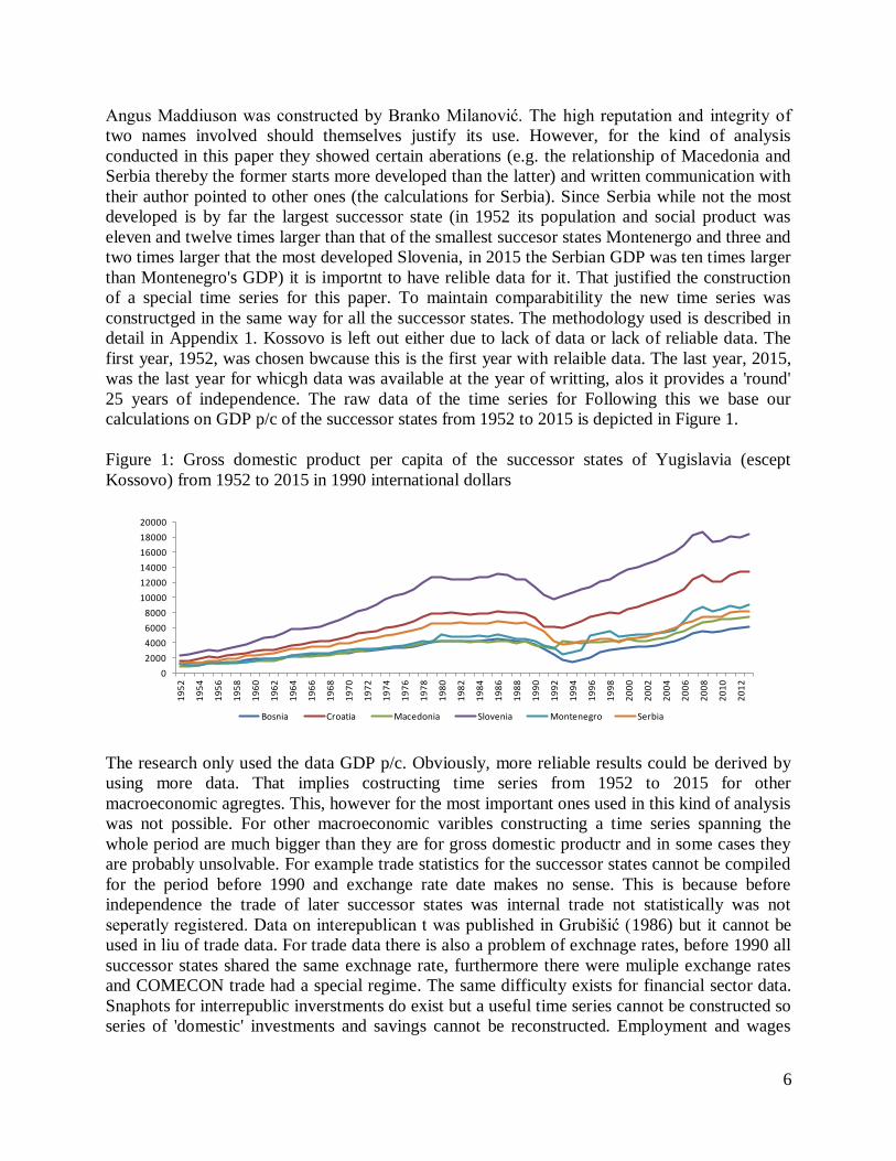
calculations on GDP p/c of the successor states from 1952 to 2015 is depicted in Figure 1.
Figure 1: Gross domestic product per capita of the successor states of Yugislavia (escept
Kossovo) from 1952 to 2015 in 1990 international dollars
The research only used the data GDP p/c. Obviously, more reliable results could be derived by
using more data. That implies costructing time series from 1952 to 2015 for other
macroeconomic agregtes. This, however for the most important ones used in this kind of analysis
was not possible. For other macroeconomic varibles constructing a time series spanning the
whole period are much bigger than they are for gross domestic productr and in some cases they
are probably unsolvable. For example trade statistics for the successor states cannot be compiled
for the period before 1990 and exchange rate date makes no sense. This is because before
independence the trade of later successor states was internal trade not statistically was not
seperatly registered. Data on interepublican t was published in Grubišić (1986) but it cannot be
used in liu of trade data. For trade data there is also a problem of exchnage rates, before 1990 all
successor states shared the same exchnage rate, furthermore there were muliple exchange rates
and COMECON trade had a special regime. The same difficulty exists for financial sector data.
Snaphots for interrepublic inverstments do exist but a useful time series cannot be constructed so
series of 'domestic' investments and savings cannot be reconstructed. Employment and wages
0
2000
4000
6000
8000
10000
12000
14000
16000
18000
20000
19
52
19
54
19
56
19
58
19
60
19
62
19
64
19
66
19
68
19
70
19
72
19
74
19
76
19
78
19
80
19
82
19
84
19
86
19
88
19
90
19
92
19
94
19
96
19
98
20
00
20
02
20
04
20
06
20
08
20
10
20
12
Bosnia Croatia Macedonia Slovenia Montenegro Serbia

7
data presents least problems. It could be reconstructed if private sector employment especially in
agriculture was recalculated. This could be done but given the notorious difficultiues of defining
the agricultural surplus in peasant farming, and private sector agriculture in Yugoslavia was only
peasant farming, the task is not straightforward. Data for some sectors is not comparable due to
the private sector (trade, agriculture, crafts). The least problem in reconstructing historical series
would be for employment and wages in sectors where the private sector was not present (e.g.
manufacturing and minning) but this is highly correlated with GDP and so of limited use for the
purpose of this research. Regarding net wages nad wage inequality example of a analysis of
secular changes in Croatia was made by Hofman et al. (2012).
3. BREAK POINTS
The economic history of Yugoslav successor states from 1952 to 2015, the time span included
here, was unquestionably turbulent. There were frequent institutional changes, almost continuous
destabilization shocks, reflexive stabilization policies and a continuum of political tensions not to
mention a regime change and the decomposition of the country with its consequences and
subsequent Wars of the Yugoslav Succession. There were also multiple internal non-economic
shocks (the death of Josip Broz Tito, droughts, etc.). To this one must add external shocks
(cycles, oil crises, cold war tensions, etc.). In short, this was a time of almost continuous change.
Under such circumstances it was a great challenge to find break points. With most of the
research done by Yugoslav or foreign political scientists, e.g. Ramet (1992) and Bilandžić
(1985).historians, e.g. Lampe (2000) or Goldstein and Goldstein (2015), descriptive economists,
see Pailaret (1997) and Sirotković (1990), and many journalists, the dominant approach was
primarily narrative and a concentration on the impact of events, more precisely of internal
political, policy or institutional shocks. In this section we take a different approach. Here we
apply standard econometric tests for determining break points in time series of GDP per capita
series for Yugoslav successor states. This approach has not been attempted till now.
Break points are defined as points in a time series in which there is a detectable change in
equation parameters according to some criteria. The first generation of tests allowed the
existence of only one break point but later econometric techniques allowed for the determination
multiple break points in the time series. The first attempt was the procedure devised by Chow
(1960) where break points are externally and ad hoc chosen and econometric procedures used to
tested for their existence. The next step was the Quandt-Andrews test aimed at eliminating the ad
hoc feature. In this test the Chow test was sequentially applied for all data points. The criteria for
the break point remained unchanged. After that theoretical work concentrated on introducing the
criteria for determining multiple break points. This was done by the Bai-Perron test. This test
recalculates the data and determines the break points for the recalculated series. The Bai-Perron
test does however require an ad hoc assumption regarding the maximum number of possible
break points the recalculation can recognize and a choice of lags.
Both single and multiple breakpoint tests were applied to the time series of GDP per capita for
Yugoslav successors states (how the series was derived from primary data is explained in the
previous section and in detail in Appendix 1). The methodological basis, i.e. the equation, used
in the paper for determining the two types of break points are described in Appendix 2.

8
3.1 Single break point analysis 1: Quandt-Andrews test and Bai-Perron test for one break
point
Single break points were determined by two different procedures. The first was the
chronologically older Quandt-Andrews test, the second was the Bai-Perron test with one break
point. The difference is that the former procedure only uses the raw data while the second
introduces lags and recalculates the original series.
The Quandt-Andrews test was the first test designed to recognize break points. The test allows
the recognition of only one break point. It is usually used to estimate the existence and timing of
one structural change in OLS estimated parameters. Using the methodology described in A2.1
and the equation A2.1 for the GDP per capita growth rates determined as in Appendix 1. Table
3.1 summarizes the results.
Table 3.1 Single break points: Quandt-Andrews test in GDP growth rates for successor states
1952-2015
SINGLE BREAK POINT
Bosnia and Herzegovina 1996
Croatia 1964
Macedonia 1982
Montenegro 1980
Serbia 1960
Slovenia 1980 Source: authors
Looking at these break points three things stand out. First, it is clear that their range is very wide,
36 years from 1960 for Serbia to 1996 for Bosnia and Herzegovina. Second, the three larger
successor states with the greatest weights have no common break points. Third, all three small
successor states have a joint break point in 1980 and 1982. Given these results and the known
turbulence of the period it seems much more probable that there were multiple break points.
The second procedure for determining a single break point uses the Bai-Perron procedure which
recognizes only one possible break point. This procedure uses formula A2.2 and the results are
given in Table 3.2.
Table 3.2 Single break points: Bai-Perron test in GDP growth rates for successor states 1952-
2015
SINGLE BREAK POINT
Bosnia and Herzegovina 1979
Croatia 1964
Macedonia 1966
Montenegro 1984
Serbia 1981
Slovenia 1966

9
Source: authors
The Bai-Perron break point tests for one break point are in a wide 20 year range between 1964
(Croatia) and 1984 (Montenegro). All the break points are in the Yugoslav period of the
successor states development and the dominant period are the mid sixties when there were 3
break points (Croatia, Macedonia and Slovenia). Two break points were around 1980 (Bosnia
and Herzegovina and Serbia). As will be clear later both these periods support the narrative
explanation but omit independence, transformation and war as influencing break points.
Comparing the two procedures shows that the only for Croatia the break points is the same in
both procedures, for the other 4 successor states the differences break points are dramatic. For
Quandt-Andrews the dominant dates are the early eighties, for Bai-Perron the mid sixties. What
is common is that neither procedure recognizes independence of transformation related dates as
break points.
With this in mind the authors consider the identification of multiple break points a more
meaningful approach.
3.2 Multiple break point analysis 2: Bai-Perron test for multiple breakpoints
The disadvantage of recognizing one break point is overcome by the Bai-Perron test for multiple
break points. The test requires that the lag and the largest number of possible break points must
be externally determined. In the test conducted here the chosen maximum was 5 break points.
Results from the Bai-Perron structural break test show multiple breakpoints in the individual
growth rates of Yugoslavia’s successor countries during the period from 1952 to 2015.
The years of the estimated break points are given in Table 3.3.
Table 3.3 Structural break dates (Bai-Perron test) for the successor states using the whole
sample, period 1952-2015
. 1960.1969 1970-1979 1980-1989 1990-1999 2000-2015
Bos. & Her 1967 1978 1995 2004
Croatia 1965 1981 1992 2007
Macedonia 1965 1980 1993 2002
Montenegro 1965 1985 1994 2007
Serbia 1965 1980 1994 2003
Slovenia 1965 1980 1993 2007 Source: authors
The results from Table 3.3 are clearer if shown in graphs. This was done in Figure 3.1. Here the
blue lines are the actual growth rates and the red line the estimated growth rates from formula
A2.2. The equation is constructed in such a way so that it allows multiple changes in its
parameters through different time periods. Thus, the red line on the picture depicts the estimated
sudden changes in the underlying evolution of GDP growth rates. The estimated years for the
break points are given in Table 3.3.

10
Figure 3.1: Multiple break points (Bai-Perron test) in GDP growth rates for successor states
using the whole sample 1952-2015
Source: authors
The above six figures for the individual successor states are clearer if they are grouped into the 3
more developed and 3 less developed successor states (the more developed are defined as above
the Yugoslav average). The results are presented in Figure 3.2 and Figure 3.3.
b) Bosnia and Herzegovina
a) Croatia
d) Macedonia
c) Montenegro
f) Serbia
e) Slovenia

11
Figure 3.2: Multiple break points (Bai-Perron test) in GDP growth rates for the more developed
successor states using the whole sample 1952-2015
Source: authors
Figure 3.3: Multiple break points (Bai-Perron test) in GDP growth rates for the less developed
successor states using the whole sample 1952-2015
Source: authors
The results are clearer if they are depicted in figures showing number of breaks. Figure 3.4
summarizes the breakpoint according to five year periods and decades and Figure 3.5 according
to individual years.
-0.1
-0.05
0
0.05
0.1
0.15
1953
1957
1961
1965
1969
1973
1977
1981
1985
1989
1993
1997
2001
2005
2009
2013
Croatiaf Serbiaf Sloveniaf
-0.3
-0.2
-0.1
0
0.1
0.2
1953
19
56
1959
19
62
1965
19
68
1971
19
74
1977
19
80
1983
19
86
1989
19
92
1995
19
98
2001
20
04
2007
20
10
2013
B&HF Macedoniaf Montenegrof

12
Figure 3.4: Bai-Perron break points distributed according to (a) five year periods and (b) decades
Source: authors
Figure 3.5: Bai-Perron break points distributed according to years
Source: authors’ calculations
Figure 3.4 shows there was an equal number of break points (six) in the sixties, nineties and after
2000. During the seventies there were least (1) break points. During the eighties there was one
break point less (5). After seventies when there was only one break point there is a rising trend of
break points during the ensuing decades. Interestingly, with the political stability i.e. following
the end of the Wars of the Yugoslav succession and establishment independence the number of
break points does not change but they are over a longer period (7) years than earlier (in the
seventies, eighties and nineties 3, 5 and 3 years respectively). Considering shorter periods the
break points are groups around the mid-sixties (6) with the dominant year 1965 (5), the early
eighties (6) with the dominant year 1980 (3), early mid-nineties (6) with no clear dominating
year and 2007 (3).
4
1 1 1
3
1 1 1 1
2 2
1 1 1 1
3
0
0.5
1
1.5
2
2.5
3
3.5
4
4.5
1953
1956
1959
1962
1965
1968
1971
1974
1977
1980
1983
1986
1989
1992
1995
1998
2001
2004
2007
2010
2013
Number of breaks
b) Five year periods
a) Decades

13
Chronologically, the first sudden change in the growth regime occurred in the mid-sixties. In all
successor states this structural break in economic growth was also a regime change accompanied
by a decline in growth rates for all successor states. Until the early 1960’s (the period 1953-1960
or 1953-1965) the average growth rate was around 7% and after 1965 (the period from 1965 to
1980) the average decreased to 5%. Furthermore, the deceleration in growth rates was
accompanied by a decrease in the volatility of economic growth which occurred for most of the
studied successor states, see Table 3.4. The fall in volatility signified a lower but more stable
growth path for these countries. Our methodology recognized the break in volatility of economic
growth for Bosnia and Herzegovina, Croatia, Serbia and Slovenia and descriptive statistics show
that Montenegro also established more stable economic growth rates during the 1960-ies (Table
3.4). Descriptive statistics show that high volatility of growth rates similar to the 1950-ies
returned again during the tumultuous 1990-ies when the first years of transformation coincided
with independence and the Wars of the Yugoslav succession. In view of this, the early 1960’s
break point may be viewed as a transition period to more stable growth rates and the nineties as a
temporary return to volatility. During the whole 39 year ‘socialist’ period there were altogether
12 break points and during 25 year ‘capitalist’ were the same number of break points.
Table 3.4: Decadal standard deviations in GDP growth rates for Yugoslav successor states
B.& H Croatia Maced. Monten. Serbia Slovenia Yugosl.
1950’s 0.13 0.08 0.06 0.14 0.14 0.05 0.08
1960’s 0.04 0.03 0.10 0.04 0.04 0.04 0.04
1970.s 0.02 0.03 0.01 0.02 0.02 0.02 0.02
1980.’s 0.05 0.03 0.05 0.03 0.03 0.03 0.03
1990’s 0.30 0.10 0.05 0.13 0.10 0.08 0.08
2000’s 0.04 0.04 0.03 0.05 0.03 0.04 0.04
2010’s 0.01 0.02 0.02 0.03 0.02 0.02 0.02 Note: Yugoslavia is the sum of real GDP of the studied countries
Source: authors’ calculation
After the early sixties the analysis of multiple break points in the growth path of the successor
states indicates the next cycle of break points in the growth regime that was common for all but
one of Yugoslavia’s successor states was around 1980. The exception is Bosnia and Herzegovina
that experienced a break point two years earlier, in 1978. This structural break was accompanied
by a huge decrease in average growth rates for these countries, from an average of 5% per
annum in the 1970’s to 0% during the 1980’s. Even though economic growth collapsed after the
break point of the early eighties, GDP per capita growth rates did not show the instability which
was characteristic for 1960’s and 1990’s.
The next break point of the successor states in the early nineties can be viewed in a wider
context. First, in a wider international context and second in a narrower ‘Yugoslav’ context.
International evidence on growth episodes (Berg, Ostry and Zettelmeyer, 2008) identified the
first half of the 1970s as a structural break for high income countries (the end of ‘Golden
growth’); the period between 1978 and 1983, for Latin America; the 1970s and the first half of
the 1980s, for Africa. So, the date of Yugoslavia’s and its successor states down-break in
economic growth roughly corresponds to the one experienced in Latin America and Africa. In a
Yugoslav context this was a period of policy shocks discussed in Section 5.

14
3.3 Summarizing the results of measured break points
The Yugoslav successor countries exhibited unstable economic growth rates during the whole
period from 1952 to 2015 but the variation among them decreased. Economic growth was
subject to sharp changes which altered the growth pattern that followed after these structural
breaks.
Chronologically, the first abrupt change in economic growth follows the break points that can be
recognized in the second half of the 1960-ies. The second wave of breakpoints that emerged
from our analysis is roughly placed in the early 1980-ies. Around this date economic growth
stopped in Yugoslavia and thus in its successor states and was followed by disintegration of
federation as the existing economic system did not manage to generate economic growth
afterwards. Interestingly, our methodology recognizes the first part of the tumultuous 1990-ies as
a continuation of the growth regime in the 1980's. Only in the mid 1990-ies economic growth
picked up again and is recognized as a start of the new economic growth regime. There was
another wave of breakpoints after 2000 but in only two successor states was it linked to the Great
Recession.
For the two more developed successor states (Slovenia and Croatia) two break points can
certainly and another one perhaps be linked to international cycles. After independence in 1990
the waves of breakpoints are wider. Two events in the world economy that are not reflected in
breakpoints is the Oil cries and the Great moderation.
4. CONVERGENCE
In the context of the secular economic development of Yugoslavia’s successor states an analysis
of economic convergence is as important as the previous discussion of break points.
Convergence can be discussed in two contexts.
The first concerns the mutual relationship of the successor states, first as republics of the
Yugoslav federation and after 1990 for 5 and eventually for 7 independent states. Two aspects
stand out. First, how did the relationships in levels of development levels of all the successor
states taken together change, was it reduced implying convergence or did the differences increase
implying divergence. Especially how did the multiple shocks of the transformation,
independence, war and EU integrations influence the relationships. This approach to
convergence is the ‘classical approach’ implied by the ‘canonical’ neoclassical one sector growth
model (the ‘Solow’ model). The model provides the theoretical background for expecting
economies to converge over time so that their differences in levels of development decrease.
Such convergence is possible only if less developed successor states have higher growth rates
than more developed ones and if the dispersion of growth rates and income per capita decrease
over time. The first convergence measure is called absolute β-convergence and the second σ-
convergence. In the first approach convergence concerns all the successor states.
The second approach to convergence considers the possible convergence or divergence of pair’s
of growth paths. Again two aspects’ are considered. The first looks at a pairs of successor states
and measures whether they converge or diverge from another one. This is important since such

15
comparison of pairs allows the identification of possible convergence clubs among successor
states, not only if they existed but whether these clubs are stable during the period or did their
composition change. The second aspect compares the growth path of successor states with the
growth path of an ad hoc chosen benchmark country. Two such benchmarks are ‘natural
candidates’ and were chosen, the first is Austria and the second Greece. Both benchmarks are
economies that during the period grew successfully. The first benchmark, Austria is a member of
the European core economies, three successor states and parts of one were in the Austro-
Hungarian Empire and hence referred to it when looking at their own development and finally it
has a psychological appeal as a benchmark. Greece was less developed but after 1974 when it
became a member of the EU it enjoyed the advantages of EU membership and redistributions
and became part of the EU convergence club, see Gill and Inderdit (2014).
The chosen approach to convergence described above required using more than one approach.
The equations used are standard in the literature so here already derived and tested. The more
detailed explanation of the equations used here are given in Appendix 3. Only the results of these
tests are described in the section while the numerical results are in the Appendix 3.
4.1 σ-convergence: the results
The first convergence measurement is σ-convergence. It is the least sophisticated measurement
but used here because there is a long tradition of measuring σ-convergence (σ is used because the
measure is the standards deviation of average per capita income in the successor states) among
Yugoslav republics and autonomous provinces till 1990. σ-convergence of social product per
capita for republics and autonomous provinces appeared in official documents, see SIV (1988) or
Uredništvo (1986) as well as all previous six five year plans, semi-official publications, see
Uredništvo (1988) and research articles and monographs, see Bogunović (1985). Foreign
analysts also initially used σ-convergence, see Ottolenghi and Steinherr (1993). Using the results
of σ-convergence led to the identification of a stylized fact about Yugoslav economy, namely
that spatial differences increased and that Yugoslavia was not a ‘convergence machine’ in spite
of a complex system of support for the less developed regions and reiterated policy
proclamations in all official documents.
Here σ-convergence is measured differently because it is measured for successor states (meaning
Serbia and Vojvodina are taken together) and Kosovo is left out (due to data issues). The results
for σ-convergence are depicted in Figure 4.1. We can see that in ‘Yugoslav’, i.e. pre-1990
period, income differences were continuously rising just as the stylized fact would have it. There
were two brief exceptions in 1962-1964 and 1978-1980. During 1980s income differences were
relatively stable, moving around the level from the beginning of 1970s. In the last years of 1980s
we can see gradual increase of income differences which temporarily and slightly decreased in
1991. With independence after 1990 from 1991 to 1994 σ-convergence increased dramatically
reaching its historical highs in 1994, no doubt due to the Wars of the Yugoslav succession. After
this maximum value σ-convergence started falling thus reflecting convergence. Eventually, by
the end of the period it reached levels similar to ones in the early eighties.
Coinciding with the global crisis at the beginning of 2000s, income differences started to rise
again, while after 2003 we could see strong compression of income differences, as a result of
convergence of less developed successor states toward its developed peers. After 2009 we can

16
see gradual reduction of income differences as Croatia, Slovenia and Serbia recorded prolonged
fall and/or stagnation of per capita income, while other countries kept strong economic
performance.
Figure 4.1: σ-convergence 1952-2015
Source: authors
These two periods of σ-convergence are clearer if the data of Figure 4.1 is divided into the two
periods. This was done in Figure 4.2 (the data from 1990 to 1995 was omitted because of the
spike but this does not change the results.
Figure 4.2: σ-convergence for sub-periods: (a) ‘Yugoslav’ 1952-1990, (b) ‘independent’ 1995-
2015
Source: authors
The changes in σ-convergence over the whole period indicate an interesting result.
Taking the whole ‘socialist’ or Yugoslav period from 1952 to 1990 there was a steady increase in
the standard deviation implying σ-divergence. This result is in line with the mentioned stylized
fact. For the second period the result is unexpected. For the ‘capitalist’ or independent period
there is σ-convergence.
0.00
0.05
0.10
0.15
0.20
0.25
19
52
19
56
19
60
19
64
19
68
19
72
19
76
19
80
19
84
19
88
19
92
19
96
20
00
20
04
20
08
20
12
d) 1952-1990
c) 1995-2015

17
4.2 β-convergence: the results
A more robust analysis of convergence is by looking at absolute, unconditional, β-convergence.
This convergence is estimated from equation A3.1 explained in Appendix 3. The equation was
tested for the data set for the Yugoslav successor states (how these values were derived is
explained in Appendix 1). Like before the present territory of the successor states is taken as the
data points (Serbia is treated in its present borders i.e. as the sum of what used to be called
‘Serbia proper’ and Vojvodina) but Kosovo is omitted due to the lack of data.
For each successor state the average growth rate is calculated from 1952 to 2015. These growth
rates are then plotted against the initial, 1952, level of per capita income. Only if the slope of the
regression line is negative is there is absolute β-convergence since such a slope implies less
developed economies have higher growth rates and are decreasing the lag behind developed
successor states. In all other cases there is no convergence and the economies are not converging
to a common growth path.
Absolute β-convergence for the period is calculated in two ways. The first is for the whole period
from 1952 to 2015 and these results are given in Fig 4.3. The line is almost horizontal indicating
virtual absence of any convergence among the successor states over the whole period. The
absence of absolute β-convergence in the regressions indicates there is no common growth path
for the successor states. During the period the successor states with higher levels of per capita
income grew faster than their less developed peers (had Kosovo been included the divergence
would have been even more pronounced).
Fig 4.3 Regression lines for absolute β-convergence 1952-2015
Source: authors
The second approach is by identifying the two periods whose existence was indicated by σ-
convergence. The first is the ‘socialist’ and Yugoslav period from 1952 to 1990, these results are
in Figure 4.4(a), and the second is the ‘capitalist’ and independent period from 1990 till 2015,
these results are in Figure 4.5(a). The absolute β-convergence of each of these periods is
different.
Convergence during the ‘socialist’ and Yugoslav period from 1952 to 1990 is depicted in Figure
4.4(a). The regression line has a positive slope implying there was no absolute β-convergence. At
that time federal republics (except for Serbia composed as previously described) with higher
y = 1E-06x + 0.0309 R² = 0.0401
2.0%
2.5%
3.0%
3.5%
4.0%
0 500 1000 1500 2000 2500

18
incomes had higher growth rates. The discussion of break points in section 3 indicated 1980 is
the most common break point during the whole period. However, this break point did not
influence absolute β-convergence during the ‘socialist’ period. This is visible in Figure 4.4(b)
where the regression line also has a positive slope indicating divergence. The period from 1952
to the first break point in 1980 has another interesting feature. Growth rates were significantly
higher than after it so the regression line is higher.
Fig 4.4 Regression lines for absolute β-convergence 1952-1980 (a) and 1952-1990 (b)
Source: authors
Calculating β-convergence for the whole second ‘capitalist’ and independent period are depicted
in Figure 4.5(a). In Figure 4.5(a) the regression line is falling which indicates indicates there was
absolute β-convergence during the whole ‘capitalist’ period from 1990 to 2015. This is also true
if the period is trimmed in two ways. First the ‘war’ years 1990-1995 and the post-Recession
years after 2008 are excluded and the period reduced to 1995-2008, the result are in Figure 4.5
(b). Then only the ‘war years’ were excluded and the period reduced to 1995-2015, the results as
seen from Figure 4.5(c). In all three cases there is β-convergence, the differences among the
economies were decreasing
Figure 4.5: Regression lines for absolute β-convergence during selected post 1990 periods: (a)
1990-2015, (b) 1995-2008 (c) 1995-2015
Source: authors
a) 1952-1980
b) 1952-1990
a) 1990-2015
b) 1995-2008

19
(c) 1995-2015
Source: authors
The final β-convergence result uses 1980 as a break point. The results for the first period from
1952 to 1980 are given Figure 4.6(a) and they show strong divergence. For the second period
from 1980 to 2015 this means combining ‘late socialist years’ after 1980 and ‘post-socialist
years’ till 2015. Results presented in Figure 4.6(b) show that from 1980-2015 there was no
absolute convergence or divergence as the slope of regression line is flat.
Figure 4.6: Regression lines for absolute β-convergence (a) 1952-1980 and (b) 1980-2015
Source: authors
It is usual to analyze β-convergence on as large a data sample as possible since this gives greater
reliability to the estimated regression and robustness to the result. It is not unusual to include
more than 100 economies. Here only 6 data points are used, one for each successor state. The
reasons for this restricted approach are twofold. First, prior to 1990 the successor states were
constituent parts of Yugoslavia and it would seem wrong to ‘mix’ them up with independent
states since they had no economic sovereignty (it would be like mixing Bavaria, Scotland,
Denmark and Portugal into a β-convergence regression). Second, one of the central results
concerns of the paper is the effect of independence and the changing patterns of convergence
under its influence. Using a larger data set would prevent deriving these results.
y = -3E-06x + 0.0609 R² = 0.5512
0.0%
1.0%
2.0%
3.0%
4.0%
5.0%
6.0%
7.0%
0 2000 4000 6000 8000 10000 12000
a) 1952-1980
b) 1980-2015

20
4.3 Pair convergence of successor states: results
In this section we will present the results of the second approach to convergence. This approach
compares growth trajectories of pairs of economies. This is done in two ways. To do this we
estimated the equation A 3.3 for the Bai-Perron test in two ways. The first was for all pairs of
successor states, i.e. for income differences between all pairs of successor states. The second way
was by comparing growth to the ad hoc chosen benchmarks.
This approach enables us to distinguish between six possible cases depicted in Figure 4.8 where
Croatia us used as merely as an example. The first case, Fig 4.8(a) is when growth paths coincide
and convergence has been completed. In Fig 4.8(b) growth trajectory are parallel with and there
is neither convergence or divergence which means that country of interest and its pair have
similar growth rates on different levels of per capita income. The next two cases are
convergence. It is possible to have convergence ‘from below’ as in fig 4.8(c) when the economy
in question is through higher growth rates converging to its benchmark, this is also ‘good or
positive’ convergence since there is ‘catch-up’. The next case, Fig 4.8(d), is convergence ‘from
above’, when the country of interest is converging due to slowing down and decreasing growth
rates. Because this convergence is generated by deceleration this is ‘negative’ convergence. The
last two are cases of divergence. In Fig. 4.8(e) which can be called ‘positive’ divergence the
country of interest begins on a similar level of income as its pair but begins to grow faster and
‘leaves its pair behind’. Finally there is ‘negative’ divergence as in fig 4.8(f) where the country
of interest falls behind of its pair.
Figure 4.8 Classification of convergence cases
Source: authors
21
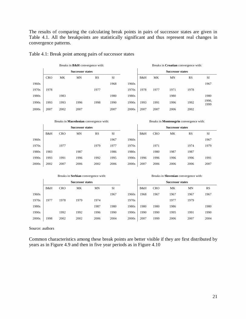
The results of comparing the calculating break points in pairs of successor states are given in
Table 4.1. All the breakpoints are statistically significant and thus represent real changes in
convergence patterns.
Table 4.1: Break point among pairs of successor states
Breaks in B&H convergence with:
Breaks in Croatian convergence with:
Successor states
Successor states
CRO MK MN RS SI
B&H MK MN RS SI
1960s
1968
1960s
1967
1970s 1978
1977
1970s 1978 1977 1971 1978
1980s
1983
1980
1980s
1980
1980
1990s 1993 1993 1996 1998 1990
1990s 1993 1991 1996 1992 1990,
1999
2000s 2007 2002 2007
2007
2000s 2007 2007 2006 2002
Breaks in Macedonian convergence with:
Breaks in Montenegrin convergence with:
Successor states
Successor states
B&H CRO MN RS SI
B&H CRO MK RS SI
1960s
1967
1960s
1967
1970s
1977
1979 1977
1970s
1971
1974 1979
1980s 1983
1987
1986
1980s
1980 1987 1987
1990s 1993 1991 1996 1992 1995
1990s 1996 1996 1996 1996 1991
2000s 2002 2007 2006 2002 2006
2000s 2007 2006 2006 2006 2007
Breaks in Serbian convergence with:
Breaks in Slovenian convergence with:
Successor states
Successor states
B&H CRO MK MN SI
B&H CRO MK MN RS
1960s
1967
1960s 1968 1967 1967 1967 1967
1970s 1977 1978 1979 1974
1970s
1977 1979
1980s
1987 1980
1980s 1980 1980 1986
1980
1990s
1992 1992 1996 1990
1990s 1990 1990 1995 1991 1990
2000s 1998 2002 2002 2006 2004
2000s 2007 1999 2006 2007 2004
Source: authors
Common characteristics among these break points are better visible if they are first distributed by
years as in Figure 4.9 and then in five year periods as in Figure 4.10

22
Figure 4.9: The yearly distribution of break points among successor states
Source: authors
Figure 4.10: The distribution of break points among successor states in five year periods
Source: authors
The yearly maximum number of break points is given in Table 4.2.
Table 4.2: Years with largest number of break points among successor states
2007 5
1967 4
1980 4
1996 4 Source: authors
Finally the break points from Table 4.1can be depicted for each successor state in Figure 4.11. A
rising trend implies divergence and a falling one convergence.
0
1
2
3
4
5
6
1952
1955
1958
1961
1964
1967
1970
1973
1976
1979
1982
1985
1988
1991
1994
1997
2000
2003
2006
2009
2012
2015
Number of breaks successor states
0 0 0
5
2
11
1
6 7
6
4
8
0 0
2
4
6
8
10
12
1950
-195
5
1956
-196
0
1961
-196
5
1966
-197
0
1971
-197
5
1976
-198
0
1981
-198
5
1986
-199
0
1991
-199
5
1996
-200
0
2001
-200
5
2006
-201
0
2011
-201
5
Number of breaks successor states

23
Figure 4.11: Breaks in convergence among successor states
Source: authors
When considering the years with the most breakpoints the following features can be seen. With
regards to 1965 the shocks mostly hit Bosnia and Herzegovina that country lost its relative
position in front of Macedonia and Montenegro while Slovenia and Croatia mostly benefited
from that shock as they accelerated its positive divergence path. The shock of 1980 is specific
because it had similar effect on most of successor states thus causing different growth paths to
‘converge’ so that after it parallel growth paths prevail. The exception is Bosnia and
Herzegovina as it surpassed Macedonia as attained its previous position. In 1990 most successor
economies were involved in the Wars of the Yugoslav Succession. This time the exception is
Macedonia which benefited as it shortly closed the gap with more developed successor states and
permanently overtook Bosnia and Herzegovina. With the exception of Serbia all the successor
states experienced a positive shock in 1995. After that breakpoint Serbia missed that
‘opportunity’ as it permanently lost its relative position to Montenegro. But while the rest
0
0.1
0.2
0.3
0.4
0.5
0.6
0.7
0.8
0.9
1
-14000
-12000
-10000
-8000
-6000
-4000
-2000
0
2000
19
52
19
55
19
58
19
61
19
64
19
67
19
70
19
73
19
76
19
79
19
82
19
85
19
88
19
91
19
94
19
97
20
00
20
03
20
06
20
09
20
12
20
15
Bosnia and Herzegovina
BH_CRO BH_MK BH_MN BH_RS BH_SI
0
0.1
0.2
0.3
0.4
0.5
0.6
0.7
0.8
0.9
1
-8000
-6000
-4000
-2000
0
2000
4000
6000
8000
10000
19
52
19
55
19
58
19
61
19
64
19
67
19
70
19
73
19
76
19
79
19
82
19
85
19
88
19
91
19
94
19
97
20
00
20
03
20
06
20
09
20
12
20
15
Croatia
CRO_BH CRO_MK CRO_MN CRO_RS CRO_SI
0
0.1
0.2
0.3
0.4
0.5
0.6
0.7
0.8
0.9
1
-14000
-12000
-10000
-8000
-6000
-4000
-2000
0
2000
4000
19
52
19
55
19
58
19
61
19
64
19
67
19
70
19
73
19
76
19
79
19
82
19
85
19
88
19
91
19
94
19
97
20
00
20
03
20
06
20
09
20
12
20
15
Macedonia
MK_BH MK_CRO MK_MN MK_RS MK_SI
0
0.1
0.2
0.3
0.4
0.5
0.6
0.7
0.8
0.9
1
-20000
-15000
-10000
-5000
0
5000
19
52
19
55
19
58
19
61
19
64
19
67
19
70
19
73
19
76
19
79
19
82
19
85
19
88
19
91
19
94
19
97
20
00
20
03
20
06
20
09
20
12
20
15
Montenegro
MN_BH MN_CRO MN_MK MN_RS MN_SI
0
0.1
0.2
0.3
0.4
0.5
0.6
0.7
0.8
0.9
1
-12000
-10000
-8000
-6000
-4000
-2000
0
2000
4000
19
52
19
55
19
58
19
61
19
64
19
67
19
70
19
73
19
76
19
79
19
82
19
85
19
88
19
91
19
94
19
97
20
00
20
03
20
06
20
09
20
12
20
15
Serbia
RS_BH RS_CRO RS_MK RS_MN RS_SI
0
0.1
0.2
0.3
0.4
0.5
0.6
0.7
0.8
0.9
1
0
2000
4000
6000
8000
10000
12000
14000
19
52
19
55
19
58
19
61
19
64
19
67
19
70
19
73
19
76
19
79
19
82
19
85
19
88
19
91
19
94
19
97
20
00
20
03
20
06
20
09
20
12
20
15
Slovenia
SI_BH SI_CRO SI_MK SI_MN SI_RS

24
experienced a positive shock it varied in intensity. Slovenia’s and Croatia’s divergence
accelerated and the ‘positive gap’ with Macedonia and Bosnia and Herzegovina expanded when
compared to pre-1990 levels. The Great Recession shock in 2009 also hit all successor states
similarly, but it had the biggest effect on Slovenian convergence pattern as its rapid positive
divergence significantly slowed leading almost to parallel growth paths with less developed
successor states
4.4 Pair convergence of successor states and benchmarks: results
The same exercises as above can be repeated with convergence breaks of successor states and the
ad hoc chosen benchmarks: Greece and Austria. The break points of convergence pairs for
Greece and Austria are given in Table 4.3. The yearly distribution of break points is in Figure
4.12 and the distribution in five year periods on Figure 4.13.
Table 4.3: Break points in convergence pairs of successor state and benchmark
B&H Croatia Macedonia Montenegro Serbia Slovenia
Greece 1960s 1963
1970s 1979 1971 1972 1970 1974
1980s 1988 1983 1986
1990s 1992 1992 1992 1995
2000s 2007 2001, 2007 2007 2007 2007 2007
B&H Croatia Macedonia Montenegro Serbia Slovenia
Austria 1960s
1970s 1971 1978
1980s 1981 1984
1990s 1991 1991 1993 1998 1990 1990
2000s 2007 2002 2001 2007
Source: authors
Figure 4.12: The yearly distribution of break points among a successor state and benchmark
Source: authors
0
1
2
3
4
5
6
7
8
9
19
52
19
55
19
58
19
61
19
64
19
67
19
70
19
73
19
76
19
79
19
82
19
85
19
88
19
91
19
94
19
97
20
00
20
03
20
06
20
09
20
12
20
15
Number of breaks EU benchmarks

25
Figure 4.13: The five year distribution of break points among a successor state and benchmark
Source: authors
Table 4.4: Maximum number of breaks with EU benchmarks by year
2007 8
1992 3 Source: authors
The results are best seen if they are presented as figures, Figure 4.13 for Austria and Figure 4.14
for Greece. Both were drawn in the same way Figure 4.11 but this time for a successor states and
the benchmark.
Figure 4.14: Breaks in convergence among successor states and Austria benchmark
Source: authors
Looking at Figure 4.14 and the patterns of break point and convergence with Austria it can be
seen that the break in 1965 was significant for Slovenia as it started rapidly converging towards
Austria and almost closed the gap towards 1980. The 1980 break accelerated Austria’s
divergence from all successor states, with Slovenia as the ‘biggest loser’. The war,
transformation and independence shocks of 1990 also resulted with accelerated divergence. After
1995 Slovenia started to gradually converge towards Austria and Croatia shared the parallel path.
0 0 1 1
2 2 3 3
7
1
3
8
0 0
2
4
6
8
10
19
50
-19
55
19
56
-19
60
19
61
-19
65
19
66
-19
70
19
71
-19
75
19
76
-19
80
19
81
-19
85
19
86
-19
90
19
91
-19
95
19
96
-20
00
20
01
-20
05
20
06
-20
10
20
11
-20
15
Number of breaks EU benchmarks
0
0.1
0.2
0.3
0.4
0.5
0.6
0.7
0.8
0.9
1
-30000
-25000
-20000
-15000
-10000
-5000
0
19
52
19
55
19
58
19
61
19
64
19
67
19
70
19
73
19
76
19
79
19
82
19
85
19
88
19
91
19
94
19
97
20
00
20
03
20
06
20
09
20
12
20
15
Austria
BH_AUS CRO_AUS MK_AUS MN_AUS RS_AUS SI_AUS

26
The Great Recession in 2009 again resulted with accelerated divergence with Slovenia as ‘the
biggest loser’ again. All the other successor states continually diverged and neither did
independence of the 25 years of transformation generate any lasting convergence.
Figure 4.15: Breaks in convergence among successor states and Greece benchmark
Source: authors
Till 1980 Slovenia converged and Croatia had a parallel growth path to Greece with all the other
successor states falling behind. Greek membership in the EU did not affect pair convergence. In
1980 Slovenian positive divergence slowed down and negative divergence of other countries
continued or accelerated. The shocks of 1990 brought acceleration of negative divergence in all
lagging countries, while Slovenia lost its leading position. After 1995 Slovenian and Croatian
divergence slowed down while in other countries it accelerated. After 2009 all countries started
to converge towards Greece and Slovenia surpassed it after nearly 20 years
In Figure 4.16 the breakpoints among the successor states and between the successor states and
the benchmarks are depicted together in five year periods.
Figure 4.16: Incidence of successor state and benchmark break point compared
Source: authors
0
0.1
0.2
0.3
0.4
0.5
0.6
0.7
0.8
0.9
1
-20000
-15000
-10000
-5000
0
5000
10000
19
52
19
55
19
58
19
61
19
64
19
67
19
70
19
73
19
76
19
79
19
82
19
85
19
88
19
91
19
94
19
97
20
00
20
03
20
06
20
09
20
12
20
15
Greece
BH_GRE CRO_GRE MK_GRE MN_GRE RS_GRE SI_GRE
0 0 0
5
2
11
1
6 7
6
4
8
0 0 0 1 1
2 2 3 3
7
1
3
8
0 0
2
4
6
8
10
12
19
50
-19
55
19
56
-19
60
19
61
-19
65
19
66
-19
70
19
71
-19
75
19
76
-19
80
19
81
-19
85
19
86
-19
90
19
91
-19
95
19
96
-20
00
20
01
-20
05
20
06
-20
10
20
11
-20
15
Number of breaks successor states Number of breaks EU benchmarks
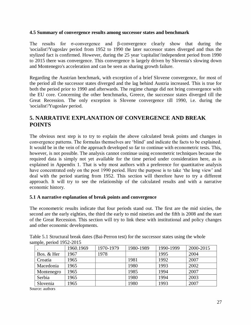
27
4.5 Summary of convergence results among successor states and benchmark
The results for σ-convergence and β-convergence clearly show that during the
'socialist'/Yugoslav period from 1952 to 1990 the later successor states diverged and thus the
stylized fact is confirmed. However, during the 25 year 'capitalist'/independent period from 1990
to 2015 there was convergence. This convergence is largely driven by Slovenia's slowing down
and Montenegro's acceleration and can be seen as sharing growth failure.
Regarding the Austrian benchmark, with exception of a brief Slovene convergence, for most of
the period all the successor states diverged and the lag behind Austria increased. This is true for
both the period prior to 1990 and afterwards. The regime change did not bring convergence with
the EU core. Concerning the other benchmarks, Greece, the successor states diverged till the
Great Recession. The only exception is Slovene convergence till 1990, i.e. during the
'socialist'/Yugoslav period.
5. NARRATIVE EXPLANATION OF CONVERGENCE AND BREAK
POINTS
The obvious next step is to try to explain the above calculated break points and changes in
convergence patterns. The formulas themselves are ‘blind’ and indicate the facts to be explained.
It would be in the vein of the approach developed so far to continue with econometric tests. This,
however, is not possible. The analysis cannot continue using econometric techniques because the
required data is simply not yet available for the time period under consideration here, as is
explained in Appendix 1. That is why most authors with a preference for quantitative analysis
have concentrated only on the post 1990 period. Here the purpose is to take ‘the long view’ and
deal with the period starting from 1952. This section will therefore have to try a different
approach. It will try to see the relationship of the calculated results and with a narrative
economic history.
5.1 A narrative explanation of break points and convergence
The econometric results indicate that four periods stand out. The first are the mid sixties, the
second are the early eighties, the third the early to mid nineties and the fifth is 2008 and the start
of the Great Recession. This section will try to link these with institutional and policy changes
and other economic developments.
Table 5.1 Structural break dates (Bai-Perron test) for the successor states using the whole
sample, period 1952-2015
. 1960.1969 1970-1979 1980-1989 1990-1999 2000-2015
Bos. & Her 1967 1978 1995 2004
Croatia 1965 1981 1992 2007
Macedonia 1965 1980 1993 2002
Montenegro 1965 1985 1994 2007
Serbia 1965 1980 1994 2003
Slovenia 1965 1980 1993 2007 Source: authors
28
5.1.1 First break points: the early and mid-sixties
After the high but erratic growth rates of the late fifties events in the early sixties took a different
course. In 1961 the economy slowed down and macroeconomic imbalances became visible. In
1960 and early 1961 policy makers were still unaware of these instabilities (at least in public),
see S.R.-D.Č. (1961). The first party meeting referring to the changed circumstances took place
in 1961, see Goldstein (2008). Instability of the early sixties is visible on three levels. The first
are changes in key macroeconomic variables, the second are policy changes and the third are
political and institutional changes.
Macroeconomic instability became visible in 1961 and can be seen in the changes of the main
variables and in their later volatility. The visible signs were rising inflation, open unemployment,
increasing foreign trade deficit and a large slowing down (deceleration) of growth with negative
growth in agriculture. Real incomes fell by -1% for the first time after 1952 Agriculture still
depended on the weather and in 1961 (when it contracted by 6%) there was a drought.
Contemporary analyst-s used this as a scapegoat for the deceleration, blaming agriculture and
weather for the economic difficulties, see S.R.-P.K. (1962).). Even though this was a modest
deceleration by later standards for contemporary circumstances it was large and had the effect of
a shock. Especially important were the shortages in raw materials and semi processed goods
which policy makers solved on an ad hoc basis and hence the witty comment that the main form
of planning and economic policy in Yugoslavia was the telephone, see Horvat (1970). The
economic slowdown continued into early 1962 and growth picked up in the second half of 1962.
The economic slowdown of the sixties led to policy reactions of all levels. There was a
stabilization policy in 1962 (the first of many to come) and plans changed. Planning priorities
shifted and administered prices including the exchange rate changed. Finally there were
institutional changes.
Economic policy changes in two senses. The first was a change in planning practices and the
second was an economic stabilization program. Planning practices also reflected the uncertainty
and imbalances. By 1962 it was obvious that the 1960-1965 five year plan could not be
implemented (in 1961 national income was 8% below planned targets and in 1962 11% below,
see Vasić (1964:377) and the plan was officially abandoned. It was replaced by yearly plans to
be followed by a seven year plan, see Sirotković (1990:89). The yearly plans were made for
1961, see B.J. (1¸961) and 1962, see M.R. (1962) and 1963, see M.R. (1963) and the seven year
plan was for 1963-1970 but it was never made public. The yearly plans mark a major shift of
investment priorities, away from machine construction and towards consumer durables. The
stabilization program of 1962 was the first in a long and almost regular sequence of stabilization
policies going on till 1994/95, first in Yugoslavia and then in successor states. The program, for
an account see Vasić (1964, 375 passim), included restrictive monetary policy (reducing
demand, especially investments, the rise in nominal wages and attempted to increase firm self
financing of working capital), exchange rate reform aimed to balance the trade balance (the dinar
devalued from 632 to 750 dinars for a dollar). This led to inflation, agricultural prices rose by
13% and cost of living by 8%, there were shortages. The policies also partly simplified foreign
trade was by introducing customs and subsidies (replacing coefficients) but trade controls

29
remained. The reform also changed accounting and firm balance sheet regulation (aimed at
limiting wages); see also S.R. (1963).
The third level of reaction to the slowdown was institutional and reflected the institutional
requirements of policy shifts. In 1963 a new constitution was passed that later inspired the
reform of 1965. With hindsight an important shift in investment policy can be seen in 1961 and
later. Considering "...in the structure of investors in 1962 the shift that started in 1961 became
even more pronounced..." S.R. (1963:115). This was the shift from federal investments
distribution to that of republics and local government. The system of investment funds was
abandoned in the 1965 reform and the federal fund closed in 1972.
The buildup of the early sixties led to the Social and Economic Reform of 1965. The narrative
history of socialist development of Yugoslavia without exception identifies 1965 as a watershed
year. Yugoslavia before 1965 and Yugoslavia after 1965 were not the same. This is true of
Yugoslav and foreign historians, see for example Goldstein (2008) and Lampe (2000), Yugoslav
and foreign political scientists, see for example Bilandžić (1985) and Ramet (2005) as well as
Yugoslav and foreign economists, see for example Sirotković (1993) and Lydall (1989). Not
only that but contemporaries also saw 1965 as a watershed year, see for example Bićanić R:
(1973), Dragosavac (1968) or Horvat (1976) and Rusinow (1977). Here we listed examples taken
from a voluminous literature but surveying this literature we did not find a single author,
Yugoslav or foreign, contemporary or more recent and regardless of her or his profession, who
would be an exception.
The system after 1965 is definitely a different system from the one of the fifties or early sixties.
The Social and Economic Reform of 1965, see Yugoslav survey (1966), was institutionally
different. State investments funds started to be phased out and they were finally closed in 1972.
Investment decisions were left to firms and administrative decisions to be financed by a
developed two tier banking systems whose importance over time rose. The scope for self
management decisions expanded to include the investment decisions, relative wages within
broad guidelines and firm independence regarding production and marketing. This all implied
expanding role of markets arbitrage. However introduction of markets was limited, foreign trade
remained regulated (through subsidies, permits and foreign currency regulation with a
administered multiple exchange rate) and there was no overt market for capital and labour, both
led to a vibrant and structurally incorporated unofficial economy, and the democratic deficit
even, though reduced, unquestionably remained. Hoping that the pro-market changes this would
lead to further expansion of markets and democracy led influential economists; see for example
Korošić (1988), to see this as a beginning of a new era. The reform momentum did not last, by
1968 political backtracking rolled back most of the changes and the search for a new paradigm
started (and was found in the associated labour institutional framework of 1974).
5.1.2 1980 the dominant year for break points
Both the econometric evidence and the narrative recognize 1980 as a clear and universal break
point. Regardless of which time series is taken (i.e. the 'socialist' 1950-1990 or historic 1950-
2014 and especially the series 1952-2008) or which formula is used and the narrative approach to
economic and institutional change all identify 1980 as a break point. This year is a break point

30
both for the Yugoslav economy and its constituent republics and later successor states. In the
whole period it is the only undisputable break point (the only exception is Croatia which had a
break point two years earlier, in 1978).
A series of events can be identified clustering around 1980 which all together through some kind
of cumulative causation can explain and justify recognizing 1980 as a break point. These events
can be divided into external and internal influences, in both cases they appear both as shocks and
as process developing over time. Not all these changes are economic.
Economists would, understandably, tend to give greater importance to economic causes of the
1980 break point. In 1980 there was, however, one non-economic shock which had an
importance that cannot be denied. This was the death of the Josip Broz Tito, President for life
and dominant figure in postwar development. Even though by the late seventies his influence
waned and he showed his age (he died 88 years old) he could still be referred to as an authority,
see Ramet (2005) and after his death there was a power vacuum. The institutional framework
was prepared for the transition to a 'post-Tito' era and there was a collective presidency with well
defined relationships of constituent parts in decision making, see Sirotković (1992). In spite of
this the death of Josip Broz did change matters for the party officials which had floated to the top
had little charisma (e.g. StaneDolanc or Josip Vrhovec) and little popular support. This could no
longer be hidden. When faced with the complex and formidable tasks of running a complicated
country in crises they were not up to the task. In this sense 1980 is the first year of the new way
of policy making.
The remaining events in the 1980 break point narrative are more in the tradition of economic
analysis. In the economic narrative of 1980 there were three events regarding the external
environment which are clearly interlinked.
The first was the perceived external soft budget constraint. Yugoslavia had a continuous external
trade deficit. From the early fifties (western aid) and especially from the mid sixties (the post
Reform commercial loans and start of 'gastarbeiter' remittances) it relied on foreign loans to
cover it. In this sense it faced policy makers perceived they faced an external and internal soft
budget constraint, any spending could be covered by loans. As a result aggregate spending was
continuously higher than production with the difference financed by loans leading to an
increasing debt. This policy collapsed by 1980 when two events coincided. The first was the size
of the debt and the second a world recession. Regarding the first "Yugoslavia's
indebtedness.[in].1979-1980 assumed proportions which exceeded possibilities for regular
repayments." (Marković:1985:51). The external liquidity crises coincided with a world recession
in 1980 and a consequent rising of interest rates on loans and drying up of the supply of new
long term loans to cover the deficit. Thus the conditions in the external environment under which
Yugoslavia could borrow changed. This was not a peculiar development for Yugoslavia as
international circumstances changed for other highly indebted countries, e.g. Mexico faced a
crises in 1981-1982. The results were twofold. First, new debt led to a predominance of short
term debts with high interest that put further strains on the trade balance deficit. Second,
creditors required an IMF standby agreement and this implied external conditionality, see
Stojanović (1991). In 1981 Yugoslavia signed its 7th standby arrangement with the IMF but its
first three year one (all the previous 6 were one year arrangements). The sole aim of this one was

31
reestablishing external liquidity and its conditionality were linked to the policies of the 1981
stabilization program. In 1982 it became clear Yugoslavia was not fulfilling its targets in the
stand-by agreement and the IMF insisted on further restrictions, see Marković:1985:455. There
are authors who see the IMF behavior with the harsh conditionality it imposed (which they see as
short sighted) as the main trigger for later unfavorable events, see Woodward (1995) and many
years later this opinion was confirmed by the then leading IMF negotiator.
External difficulties were closely reflected in internal ones. The internal reaction to the debt
crises and cumulating external and internal macroeconomic instability was twofold. The first was
a result of IMF conditionality which and imposed a stabilization policy in 1981. Its sole goal was
achieving external liquidity. The 1981 stabilization package required a devaluation (the dinar
devalued 30%) and, more importantly import restrictions (which led shortage of everyday
consumer goods, petrol rationing, limiting use of cars) and travel restriction (and travel deposit
which was an enormous psychological shock going to the very heart of Yugoslavia's special
position), etc. This policy package changed the everyday lives of all citizens. It was a shock
which remains a collective memory till today, 35 years later. The stabilization package and
policy had IMF support and was part of stand-by conditionality. The second reaction was an
attempt to face the causes of the soft budget constraint that had led to the indebtedness. This
implied institutional and structural changes. Once the ruling party (with an external nudge)
decided reforms were imminent it established a commission to propose deep reforms. The
commission completed its work in 1983 and proposed a Long term stabilization program whose
goal was to institutionally reform the economy to achieve sustainable growth. The long term
stabilization program known as the 'Report of the Kreigher Commission' presented its
recommendation in 1983 in 4 volumes, for a short survey see Budimir (1983). The proposals
recommendation stayed within the existing institutional framework (associated labour and
federal arrangements) but sought to increase the scope of markets and especially provide the
underpinnings of financial sector development (by changing interest rate determination,
exchange rate policy, inter firm financing, etc.).
While the shock therapy did achieve external liquidity and was a success (the harshest measures
were scaled down and shortages disappeared) the reforms for sustainable development were
never seriously implemented. Once the danger of external default subsided and conditionality
weakened the proposed reforms were either watered down or postponed. Finally, a new and
similar commission, this time the 'Pašić Commission', was set up in the mid eighties. Yugoslavia
backtracked on serious pro market reform.
It is important to note that economic policy makers after 1980 were losing contact with reality.
For example planning became a fiasco. The planning targets became increasingly distant from
reality. While this may be explained for the 1981-85 plan which was part of the IMF
conditionality but virtually abandoned by 1983, see Sirotković (1984), and replaced by yearly
plans there is no reason for the failure of the 1986-1990 plan which did not learn from the
mistakes. The discrepancy of targets and reality became even bigger.
5.1.3 An 'obvious' point of discontinuity: the early mid nineties
After 1989 the economies of the successor states were suddenly and quite unprepared for
multiple shocks. First was the start of the transformation, the second the decomposition of

32
Yugoslavia, the third were the Wars of the Yugoslav Succession and finally there was the virtual
disappearance of former Comecon markets.
The transformation started in Yugoslavia in 1989 when the final economic reform this country
has equated all forms of ownership (prior to that ‘social ownership’ had a special privileged
position) and institutionalized a process of gradual privatization. These reforms broke the
ideological barriers but the transformation itself got under way once the country decomposed, i.e.
after 1990. It is worth noting how quickly the successor states chose different policy options to
deal with the three fundamental transformation generated process: privatization large and small,
financial sector consolidation and economic stabilization, see Bićanić (1996). In spite of 72 years
of sharing and institutional and economic space (with the exception of 4 years during the Second
World War) within a couple of years they were recognizably different economies.
The decomposition of Yugoslavia started with the independence referendums in Croatia and
Slovenia in 1990 and ended with the recognition of independent Kosovo Declaration of
Independence in 2008. The dominant year of decomposition was 1991 when 5 successor states
were internationally recognized. Serbia and Montenegro split in 2006 so finally the
decomposition spawned 7 successor states, even though at least 2 remain dysfunctional states
and international protectorates. The way the decomposition developed in did severe many
previously built economic ties. Even though the level of economic integration and its changes
were a hot topic of discussion prior to the decomposition mutual trade was never separately
accounted, the nearest are inter-republic deliveries for two years, see Grubišić (1990). This data
shows that a sudden stop in these economic links should have a major disruptive effect on the
successor states.
The Wars of the Yugoslav Succession started with the ’10 day war in Slovenia’ in 1991 and
ended with the NATO bombings of Serbia in 1999. Two important interim dates were the
Dayton Peace Accords in 1995 and in 1998 the Peaceful reintegration of Western Srijem and
Eastern Slavonia. The brunt of the military conflict was, however, in Croatia and Bosnia and
Herzegovina from 1991 to 1994 and Slovenia and Macedonia were least affected but it seems
obvious that this was a major shock for all successor states.
The final shock was external and resulted from the transformation and its consequences in
Eastern and Central Europe. These were important export market for the successor states and the
cutting of established economic flows was an asymmetric shock because of different exposure of
successor states to this trade but still a shock.
5.1.4 The selective impact of the great recession and national specifics
The first decade of the 21st century marked beak point for all successor states but no clear
relationship and common thread. This is in spite of the eyeballing the data that would seem to
imply commonalities, see Figure 5.1. The ‘Great Recession’ was a break point only for the two
most developed successor states, Slovenia and Croatia. These economies are also most integrated
into the international economy, at the time one already was an EU member (Slovenia) and one
already quite far in membership negotiations (Croatia). For the others the break point in this
decade is probably better explained by national specifics. For example for Montenegro the 2007

33
break point is growth acceleration. and the newly independent Montenegro. But the effect was
different. For the first two it was a contraction, for Montenegro a spurt of growth. For the
remaining 3 successor states the decline started earlier
Figure 5.1: Real growth rates 2000-2009 in Southeast European economies
Source: authors
5.2 Growth in sub-periods derived from the narrative approach
With the strong link between the calculated break points and the narrative it impossible to
distinguish the following periods. The names of the periods are determined only in relationship
to the average growth rates.
1. 1952-1979 period 'successful socialism'
2. 1980-1989 period 'socialist stagnation
3. 1990-1994 period 'capitalist turmoil'
4. 1995-2008 period 'successful capitalism'
5. 2009-2015 period 'capitalist stagnation'
For these periods average yearly growth rates are given in Table 5.2 and depicted in Figure 5.1.
In the figure the blue line gives the yearly rates and the red line the average yearly growth rate
for the sub-period.
Table 5.2: Average growth rates for narrative sub-periods
B. and H. Croatia Macedon. Monteneg Serbia Slovenia
1952-1979 4.8 6.4 6.0 5.5 6.5 6.5
1980-1989 0.5 0.0 -0.1 1.4 0.4 -0-3
1990-1994 -9.6 -8.7 0.8 -8.6 -10.0 -2.8
1995-2008 9.1 5.1 3.7 6.3 5.0 4.1
2009-2015 2.2 -0.2 2.5 1.1 1.2 0.6 Source: authors
The growth rates of these subperiodsshouildbe put in context of the secdular growth rate of the
whole period which are calcvulated from the lienar trend and givne in Table 5.3.

34
Table 5.3: Average growth rates 1952-2015
B. and H. Croatia Macedon. Monteneg Serbia Slovenia
1952-2015 1.94 2.88 2.77 2.95 2.15 2.84 Source: authors
Figure 5.1: Yearly growth rates and average growth rates for narrative sub periods for successor
states
Source: authors
The data shows that with the two exceptions the growth rate of 'successful socialism' is larger
than that of 'successful capitalism'. Slovenia is especially interestingly the economy frequently
referred to as 'the most successful transformation economy' actually experienced the largest
difference in growth rates during the two periods. The two exceptions are Bosnia and
Herzegovina that had the largest contraction during the Wars of the Yugoslav Succession so its
reconstruction rebound my not surprise and Montenegro. Another exception is Macedonia which
did not experience a 'capitalist stagnation'.
-40.0%
-30.0%
-20.0%
-10.0%
0.0%
10.0%
20.0%
30.0%
40.0%
19
53
19
56
19
59
19
62
19
65
19
68
19
71
19
74
19
77
19
80
19
83
19
86
19
89
19
92
19
95
19
98
20
01
20
04
20
07
20
10
20
13
Bosnia&Herzegovina
-20.0%
-15.0%
-10.0%
-5.0%
0.0%
5.0%
10.0%
15.0%
20.0%
19
53
19
56
19
59
19
62
19
65
19
68
19
71
19
74
19
77
19
80
19
83
19
86
19
89
19
92
19
95
19
98
20
01
20
04
20
07
20
10
20
13
Croatia
-15.0%
-10.0%
-5.0%
0.0%
5.0%
10.0%
15.0%
20.0%
25.0%
30.0%
35.0%
19
53
19
56
19
59
19
62
19
65
19
68
19
71
19
74
19
77
19
80
19
83
19
86
19
89
19
92
19
95
19
98
20
01
20
04
20
07
20
10
20
13
Macedonia
-40.0%
-30.0%
-20.0%
-10.0%
0.0%
10.0%
20.0%
30.0%
40.0%
19
53
19
56
19
59
19
62
19
65
19
68
19
71
19
74
19
77
19
80
19
83
19
86
19
89
19
92
19
95
19
98
20
01
20
04
20
07
20
10
20
13
Montenegro
-30.0%
-20.0%
-10.0%
0.0%
10.0%
20.0%
30.0%
40.0%
19
53
19
56
19
59
19
62
19
65
19
68
19
71
19
74
19
77
19
80
19
83
19
86
19
89
19
92
19
95
19
98
20
01
20
04
20
07
20
10
20
13
Serbia
-15.0%
-10.0%
-5.0%
0.0%
5.0%
10.0%
15.0%
19
53
19
56
19
59
19
62
19
65
19
68
19
71
19
74
19
77
19
80
19
83
19
86
19
89
19
92
19
95
19
98
20
01
20
04
20
07
20
10
20
13
Slovenia

35
5.3 Quarter of a century of independence and transformation
There are many ways the quarter of a century experience of the independence and transformation
can be tackled and evaluated. Here a very simple approach is used. The 25 year experience will
be looked at in terms of what Kuznets (1966) called Modern Economic Growth and Gershenkron
(1977) Spurt That Failed.
Kuznets defines Modern Economic Growth as persistently high levels of growth over a long
period accompanied with restructuring and structural changes in an acceptable environment. All
parts of the definition are important. Gerschenkron refers to periods of high growth rates that did
not last.
The secular growth rates 1952-2015 of the successor states are given in Table 5.3. They are
presented together with the post-conflict growth rates for the twenty-year period 1995-2015.
Table 5.3: Average growth rates 1952-2015 and 1995-2015
Successor states EU benchmarks
B. and
H.
Croatia Maced. Mont. Serbia Slov Austria Greece
1952-2015 1.94 2.88 2.77 2.95 2.15 2.84 2.79 3.15
1995-2015 6.78 3.31 3.29 4.59 3.74 2.96 2.0 1.9
Source: authors
The post conflict ‘capitalist’ growth rates in Table 5.3 are biased in two ways. In both cases they
inflate growth rates. They include the post-war reconstruction (this is especially visible for
Bosnia and Herzegovina) and start measuring growth from a trough (after the contraction of the
early nineties, this is especially visible for Serbia). Furthermore, the period includes two distinct
sub-periods that were above referred to as ‘successful’ and ‘stagnant’ capitalism see Table 5.2.
For Slovenia and Croatia they are slightly above the secular rate but the more unstable the
economy the larger the difference.
In spite of the higher growth rates they imply neither Modern economic growth nor a significant
acceleration with convergence. In terms of growth the 1995-2015 period has not been a success.
The size of the lag and the time spans involved in catching up with the European core (Austria)
are visible from the Croatian case presented in Table 5.4. Modern economic growth would
require at least 5% yearly growth rates over a long period.
Tablica 2.4:Croatia: years required to catch up with ad hoc chosen benchmarks
Slovenija (growth rate 3%)
Austrija (growth rate 1,5%)
EU average (growth rate2%)
Initial value 18 093 38 541 27 394
2% Never,
increasing lag
170 years Never
Paralel paths
3% Never 57 years 53 years

36
Paralel paths
5% 25 years 25 years 18 years
Source:authors calculations
Regarding Gerschenkron’s spurt all the successor states except Montenegro had an acceleration
that did not last. This is visible from 5.2. the required growth rates did exist from 1995 to 2008
but did not last. Furthermore the spurt led to major economic imbalances (debt, structure,
instability) which do not make them probable in the near future.
6. CONCLUDING REMARKS
The paper is based on an analysis of the per capita gross domestic product time series from 1952
to 2015 for the Yugoslav successor states (except Kosovo that is omitted due to lack of data).
Using standard econometric procedures for determining multiple breakpoints in time series, the
Bai-Perron test, and measuring convergence, of groups of countries or pairs, the results broadly
supported the results of narrative analysis and added evidence for the recognition of sub-periods.
The main breakpoints were in the mid sixties, coinciding with a major institutional reform, in
1980, coinciding with an external hard budget constraint, the early nineties, coinciding with
transformation stabilization, and the first decade of the twentieth century.
The analysis of breakpoints in addition to this support added three new insights. First, the
dominant breakpoint was 1980, not the oil crises that was the watershed for Golden age growth
in Europe, and not 1990 with its multiple shocks of transformation, independence and war.
Second, if break points can be seen as a sign of instability then the ‘socialist’/Yugoslav period
1952-1990 and the ‘capitalist’/independent period 1990-2015 are equally unstable since they
have the same number of breakpoints. Stability did not increase over time. Third, as can be
expected, with independence after 1990 the span of breakpoints increased as the independent
states choose different policy options. Finally, the Great Recession of 2008 is a breakpoint only
for the two most developed successor states and EU members (one was finalizing its membership
negotiations).
The measurement of convergence did indicate some unexpected results. Both β-convergence and
σ-convergence supported the established fact that in Yugoslavia there was no convergence but
also clearly showed that with independence both kinds of convergence developed. However, in
spite of this change over the period as a whole there was no convergence. Comparing the
relationship of pairs of growth trajectories for the 6 successor indicate instability with few
changes in structure. With the exception of the stagnant eighties when there was parallel growth
for all the more developed diverge from the less developed and the development gradient did not
change. Also the pair convergence seems to indicate the convergence was driven by Slovenia’s
deceleration and Montenegro’s catch-up. The results of comparing the growth paths of individual
successor states with ad hoc chosen benchmarks, Austria and Greece, indicate important results.
With the exception of Slovenia during a period till the eighties all successor states diverged from
the European core and increased their lag. Regarding Greece the results are more mixed,
Slovenia converged for a time and Croatia had parallel growth till the eighties, after that till the
Great Recession all diverged except Slovenia and after 2008 there was convergence.
37
The time series includes quarter of a century of independent growth. The regime change did not
produce convergence to the European core and divergence continued (the best performer
Slovenia kept its distance). Till the Great Recession this was also true for Greece. If the time
series is divided into 4 sub-periods, ‘socialist’ high growth from 1952 to 1980 and stagnation
from 1890 to 1989 and ‘capitalist’ high growth from 1995 to 2008 and stagnation from 2009 to
2015 (the period 1990 to 1995 is left out) interesting results appear. For three successor states,
Croatia, Serbia and Macedonia, the two high growth and stagnation periods are very similar. For
two, Bosnia and Herzegovina and Montenegro, the latter high growth period is significantly
higher (for Bosnia and Herzegovina this is probable reconstruction). The unexpected result is
Slovenia for which ‘capitalist’ growth is lower than ‘socialist’ growth. In terms of growth the
regime change did not generate Modern economic growth in any successor state and in terms of
growth the most developed is the only clear loser. With one exception, Montenegro, the two
stagnation periods have a striking similarity in spite of regime changes. In both cases they were a
result of an external shock, the first in 1980 and the second in 2008, sand seem to indicate that in
both cases there was an internal inability to react appropriate to these shocks.

38
REFERENCES
Antoshin Sergei, Berg Andrew iSouto Marcos (2008): Testing for Structural Breaks in Small
Samples, unpšibloisdhjed paper
Bai, J. and Perron, P. (1998): “Estimating and Testing Linear Models with Structural Changes”,
Econometrica , Volume: 66, pp: 47–78.
Bai, J. and Perron, P. (2003): “Computation and Analysis of Multiple Structural Change
Models,” Journalof Applied Econometrics, Volume: 6, pp: 72–78.
Bajt Aleksandar (1988): Samoupravnioblikdruštvenesvojine (Selfmanagement forms of social
ownership), Globus, Zagreb
Berg Andrew, Ostry Jonathan and TettelmeyerJeronim (2008): What Makes Growth Sustained?,
IMF Working Paper, WP/08/59, IMF, Washington
Bernard B. Andrew iDurlauf N. Steven (1995): „Convergence in International Output“ Journal
of Applied Econometrics, Volume: 10, Number: 2 (Apr. - Jun., 1995), pp: 97-108
Bićanić Ivo (1996): The Economics of State Building in the Former Yugoslavia, Occasional
Paper number 43, Woodrow Wilson Centre, Washington
Bićanić Ivo (1995): “The Economic Causes of New State Formation during the Transition” East
European Politics and Society, Vol: VIII (winter), pp: 2-21
Bićanić Ivo (1989): 'Jedinstvo jugoslavenskog gospoidarstva', (The unity of the Yugoslav
economy) Kulturni radnik, Volume: 42, Number: 3, pp: 1-17
Bićanić Ivo (1988): "Fractured Economy" in Rusinow, ed. (1988)
Bićanić Ivo and Tuđa Dora (2014): DugoročneserijeDBP-a Hrvatske, (Croatian long term GDP
series) Privrednakretanja I ekonomskapolitika Vol: 22, No 134
Bićanić Ivo and Škreb Marko (1994):“The Yugoslav Economy From Amalgamation to
Decomposition” in Good David, editor (1994) Economic Transformation in Central and Eastern
Europe: Lesson and Legacies from the Past, Routledge, London
BilandžićDušan (1985): HistorijaSocijalističkeFederativneRepublikeJugoslavije – glavniprocesi
(A Histroy of the Socialist Federative Republic of Yugslavia – main process) Šklskaknjiga,
Zagreb
Bogunović Aleksandar (1991): Regionalnaekonomika (Regional economics); Narodnenovine,
Zagreb

39
Bogunović Aleksandar (1985): RegionalnirazvojSocijalističkeJugoslavijeiHrvatske (Regional
development of socalist Yugoslavia and Croatia), SNL, Zagreb
Borak Neven (1992) SpočetjeEkonomskeSamostojnosti(Economic independence),
ZaložbaZnanstveno in pšublicističkosredišče, Ljubljana
Borak Neven (2002): Ekonomskividicidelovanja in raspadaJugoslavije (Economic aspects of the
functioning and breakup of Yugoslavia) ZPS, Ljubljana
ChowGregory (1960):
'TestsofEqualityBetweenSetsofCoefficientsinTwoLinearRegressions'Econometrica, Vol: 28, No:
3, pp: 591-605
Crafts Nicholas (2002): The Human Development Index 1870-1999: Some Revised Estimates,
European Review of Economic History, vol: 6, pp: 395-405
Collier Paul and HoefflerAnke (1998): The Economic Causes of civil War, 0xford Economic
Papers, Vol: 50. pp:563-573
Coyle Diane (2014): GDP: A Brief but Affectionate History, Princeton University Press,
Čobeljić Nikola (1959): PolitikaimetodiprivrednograzvojaJugoslavije, (Policy and methods of
economic development of Yugoslavia) Nolit, Belgrade
DragosavacDušan (1969): AktuelniproblemiekonomskipolitikeJugoslavije (Current problems of
Yugoslav economic policy), Informator, Zagreb
Dr. M.M. (1959): "Statističkisistem u FNRJ" (The statistical service in the FPRY),
Jugoslovenskipregled, Vol: , No: 9 (September), pp 63-7 (325-9)
DružićGordan (2009): CroatianEconomicDevelopment and the EU, Školskaknjiga, Zagreb
DružićGordan (2012): Coratian Development Through History, Montenegrian Journal of
Economics, Volume: 8, pp: 157-177
Družić Ivo iTica Josip (2002): ˝DinamikaikontroverzegospodarskograzvitkaHrvatske˝ objavljeno
u Družić Ivo, urednik (2002): Stabilizacija – participacija – razvoj,Sveučilište u Zagrebu,
Ekonomskifakultet Zagreb, strane 107-126
Dyker David (1990): Yugoslavia: SocialistmDevelolment and Debt, Rotlegde, London
Đurđević Ivanka (1987): Razvojnedovoljnorazvijenihrepublikaipokrajine Kosovo 1981-1985
ipolitikarazvoja 1986-1990 (Development of less developed republics and the propvince of
Kosovo 1981-1985), Jugoslovenskipregled, Vol: , No: 5, pp:241-254

40
Estrin Saul I Uraga Giovanni (1997): 'Testing for Ongoing Convergence in Central and Eastern
Europe' CEPRDiscussion Paper number 1615, CEPR, London
Filipović M. (1949): Stanjenašeindustrije do periodaplanskeprivrede: Drugibilans, (The state of
our indistry till the planning period: second balance) Sindikalnabiblioteka, Belgrade
Filipović M: (1946): Obnovanašeindustrija: Prvibilans, (The reconstruction of opurindistry:
First balance), Sindikalnabiblioteka, Belgrade
GerschenkronAlexander (1977): An Economic Spurt that Failed: Four Lectures in Austrian
History, Princeton –University Press, Princeton, 1977
Glenny Misha (1992): The Fall of Yugoslavia,: The Third Baslkan War, Lomndon, Penguin
Books
Goldstein Ivo i Goldstein Slavko (2015): Tito, Profil, Zagreb
GrđićGojko (1976): Makroekonomskibilansi: njihovagenzaievolucija, (Macroeconomic balances:
their genesis and evolution) SavremenaadministracijaEkopnomksiinstitut Beograd, Belgrade
GrubišićMirko (1990): Međurepubličkiprometrobaiuslugaod 1968 do 1987, (Interepublic trade
of goods and services from 1987 to 1987) Analizeiprikazi No: 73, Republičkizavodzastatistiku,
Zagreb
HanžekovićMarijan (1968): PrivrednisistemJugoslavije, (The economic system of Yugoslavia)
NarodneNovine, Zagreb
Hardt John and Kaufman Richard, editors (1989): Pressures for Reform in the East European
Economies, Vol: 1, Study Papers submitted to the Joint Economic Committee Congress of the
United States, S.Prt 101-53, Washington D.C.
Hofman Saul, Bićanić Ivo and Vukoja Oriana (2012): ‘Wage inequality and labor market impact
of economic transformation: Croatia 1970-2008’ Economic Systems, Vol: 36, No 2 (June 2012):
pp: 206-217
Horvat Branko (1989): ABC Jugoslavenskogsocijalizma (The ABC of Yugoslav socialism),
Globus, Zagreb
Jones Benjamin and Olken Benjamin (2005): The anatomy of Start-Stop Growth, NBER
Working paper 1152, NBER, Cambridge, Mass.
KitaljevićBoško (1969): SistemdruštvenihračunaJugoslavijeinjegovaevolucija, (The system of
Yugoslav social accounting and its evolution).s 1969
KorošićMarijan (1988): Jugoslavenskakriza, (The Yugoslav crises), Naprijed, Zagreb

41
KorošićMarijan, urednik (1989): Quo Vadis Jugoslavijo?Naprijed, Zagreb
Kraft, Evn (1992), “Evaluating Regional Policy in Yugoslavia, 1966–1990”, Comparative
Economic Studies, 34, 3-4, 11-33.
Krugman Paul (1996): 'Cycles od conventional wisdom on economic development' Internationla
Affairs, godište 72, broj 1, strane 717-32
Kukić Leonard (2015): Socialist growth revisited: Insights from Yugoslavia,
http://personal.lse.ac.uk/KUKIC/Kukic_SocialistGrowthRevisited.pdf
Kuznets Simon (1966): Modern Economic Growth: Rate, Structure and Spread, Yale University
Press, New Haven
Lampe John (2000): Yugislavia as Histoy: Twice there was a country, Cambridge _Ubiversity
Press, Cambridge
Maddison Angus (2002): The World Economy – a millenial perspective, OECD Development
Centre, Pariz
Marsenić Dragutin (1981): EkonomskastrukturaiprivredirastJugoslavije, (The economic
structure and economic growth of Yugoslavia) Savremenaadministracija, Belgrade
MihailovićKosta (1990): RegionalnastvarnostJugoslavije, (Regional circumstances in
Yugislavia), Ekonomika, Belgrade
MilanovićBranko (2013) u TheMaddison-Project, http://www.ggdc.net/maddison/maddison-
project/home.htm, 2013 version
Miljković Dušan (1992): ˝The Economic Development of the Former (SFR) Yugoslavia
Compared to the Countries of Europe 1985-1991˝ Yugoslav Survey, Vol: 33, No: 4, (1992), pp:
107-126
MladenovićMihailo (1981): Razvojprivrednonedovoljnorazvijenihrepublikaipokrajine Kosovo,
(Development of less developed republics and the propvince of Kosovo), Jugoslovenskipregled,
Vol: , No: 9, pp: 335-344
Muzgasova Zuzana, Ilahi Nadeem, Miniane Jacques, Scott Alasdair, Vladkova-Hollar Ivanna
(2015): The Western Ballans: 15 Years of Economic Transition, IMF Washington
Novak Mijo, editor (1971) :Tržište u višenacionalnojzajednici, (Thre market in a mutlinational
community), Institutzaekonomskaistraživanja, Zagreb
OttolenghiDanile and Steinherr Alfred (1993): Yugoslavia: Was it a Winner’s curse, Economics
of Transition, Volume 1, No: 2, pp: 209-243

42
Oulton Nicholas (2012): Hooray for GDP, Centre for Economic Perfomance, Ocassional Paper
No: 30,
Pailaret Michael (1997): The Balkan Economies c. 1800-1914 Evolution Without Development,
Cambridge University Press, Cambridge
Pleština Dijana (1992): Regional Development in Communist Yugoslavia, Westview Press,
Boulder
Popović Milenko (2010) PrivrednirastCrne Gore: Analiza, dijagnoza, alternative“, (Economic
development of Montenegro: analysis, diagnosis and alternatives) Daily Press, Podgorica, 2010
Popović Milenko and Čizmović Mirjana (2013): The Sources og Growth in the Former SFRY
Countries: Comparative Analysis, MPRA Paper 49776
PrinčičJože (1997): Slovenskogospodarstvo v drugiJugoslaviji (The slovene economy in the
second Yugoslavia), Modrijan, Ljubljana
Quandt, Richard, (1960) „Testsof the Hypothesisthat a LinearRegressionObeysTwo Separate
Regimes“, Journalof the American StatissticalAssociation. 55
Raguž, Irena; Družić, Ivo; Tica, Josip (2011) ‘Human Capital in Growth Accounting: The Case
of Croatia’, Journal of International Scientific Publications: Educational Alternatives, Vol.9 Ramet Sabrina (2004): Balkan Babel: The Disintegration of Yugoslavia from the Death of Tito to
the Fall of Milošević,4th edition, Westiew Press, Boulder. Colorado
Rusinow Dennison, editor (1988): Yugoslavia: A Fractured Federalism, The Wilson Cetner
Press, Wasghington
Rohatinski Željko, editor (1990):
AktuelniproblemiprivrednihkretanjaiekonomskepolitikeJugoslavije, (Current problems of
economic developoments and economic policy of Yufoslavia), EkonomskiInstitut Zagreb, Zagreb
Sala-i-Martin (1996): A Classical Approach to Convergence Analysis,Economic Journal, 1996,
vol. 106, issue 437
SirotkovićJakov (1990): EkonomskirazvojJugoslavije: odprosperioteta do krize, (Yugoslav
development: from prosperity ot crises) NarodneNovine, Zagreb
SirotkovićJakov (1993): Hrvatskogospodarstvo 1945-1992:
EkonomskiuzrocislomaJuglslavijeioružaneagresijenaHrvatsku (The Croatian Economy 1945-
1992: Economic Reasons behind the breakdown of Yugoslavia and the Armed Agression against
Croatia), StudijeinstitutazaekonosmskaistraživanjaHAZU, , Vol 28, HAZU, Zagreb

43
SIV (1988): AnalizaocenaistanjeprivrednestruktureJugoslavije, (Analysis, evaluation and state
of the economic structure of Yugoslavia), SIV, Belgrade
Statistical Office of the Republic of Serbia (2008): Two Centuries of Serbian Development:
Statistical Review,Republičkizavodzastatistiku, Belgrade,
Stiglitz Joseph, Sen Amartya iFotoussi Jean-Paul (2009): Report by the Commission on the
Measurement of Economic Perfomance and Social Progress, INSEE, Pariz,
Stipetić Vladimir (2012): Dvastoljećarazvojahrvatskoggospodarstva (1820-2005), (Two
centuries of Croatian economic development: 1920-2005), HAZU, Zagreb
Stock, James H. and Watson, Mark W., (2004): "Has the BusinessCycleChanged and
Why?", NBERChapters, in: NBERMacroeconomicsAnnual 2002, Volume 17, pages 159-230
National BureauofEconomic Research, Inc
St. St. (1957), 'Nacionalnidohodak 1947-1956 godine' (National income 1947-1956)
Jugoslovenskipregled, str,465-469.
Tica Josip (2004): ˝The Estimation of 1910-1989 Per Capita GDP in Croatia˝, Zagreb
International Review of Economics & Business, Volume: VII, number:1-2, pp 103-133
UNDP (1993): Human DevelopmentReport 1993, United Nations, New York
Uredništvo (1988): 'PrivrednastrukturaJugslavije 1971-1985' (The economic structure of
Yugoslavia 1971-1985), Jugoslovenskipregled, Vol: , No. 6, pp:245-262
UvalićMilica (1993): The disintegration of Yugoslavia: Its costs and Benefits, Communist
Economies and Transformation, Vol: 5, No: 3, pp:273-93
UvalićMilica (2010): Serbia's Transition, Palgrave Macmillan, London
Vinski Ivo, (1978): „Kretanjedruštvenogproizvodasvijeta od 1910. do 1975. godine“, Zagreb:
Ekonomskiinstitut Zagreb.
VojnićDragomir (1994): 'Ekonomskedimenzijedezintegracije : s
posebnimosvrtomnanekedemografske,etničkeipolitičkeaspekte’, (Economic effects of
disintegration withg special r
feference to some demographic and ethnic aspects) Ekonomskipregled,Volume: 45, Number: 3-
4/1994, pp:. 260-290.
Woodward (1995): The Balkan Tragedy: Chaos and Dissolution after the Cold War, Washington
D.C. The Brookings Institution
Ž.D. (1959): "SlužbaDruštvenogknjogovodstva" (Social Accounting Sevice),
Jugoslovenskipregled, Vol: , No: 11 (November), pp81-3 (405-7)

44

45
Appendix 1: Data and construction of time series 1952-2015
Any kind of statistical measurement crucially depends on the data used. Good econometrics does
not rely only on the correct setting of the equations and knowing their limitations but of also
knowing the value and limitation of the data used in the calculation. Thus, an awareness of the
data limitations is useful, all too often modern researchers with 'mouse pushing expertise'
download data forgetting how it was compiled. Maybe they should remember Benjamin Disraeli
who said that 'There are three kinds of lies: lies, damned lies and statistics', quoted from Huff
(1954). This appendix concentrates on the way the used data was calculated and what limitations
the procedure entails.
In the paper a time series for Yugoslavia and its successor states is derived for the period from
1952 to 2013. As a result data from three 'periods' are used. The first is data from 'socialist'
period from 1952 to 1989. The second is the data from the early nineties when the statistical
service and macroeconomic instability led to estimated values. The third is the period from the
late nineties when reliable UNSNA data was collected.
The data used in the paper spans the period from 1952 to 2013. It uses only official data,
Yugoslav data for the country and later successor states from 1952 to 1990 and data for the
successor states from 1990 to 2013. The first year 1952 was chosen for two reasons. First, that is
the first year for which data collected at the national and successor starts was collected by a
coherent system of national accounts based on the system of material balances. Second, the
institutional setting was less volatile and so the collected data is more reliable. But even for the
chosen period there are many issues that raise serious reliability questions. In spite of this the
authors think these problems are no greater than in other studies of long periods using data
before 1960 (from when the first PENNSTATEPPP estimates are available) which are
commonly used in the study of long term trends (e.g. date going back into the interwar period,
the 19th century or even earlier).
A1.1 Justifying the exclusion of data before 1952
The data before 1952 was not used to construct time series for GDP or GDP p/c of the successor
states. The period before 1952 can be divided into three sub periods.
The first one covers Yugoslav data for the interwar period (1918-1941). During this period there
were no national accounts and the collected data does not permit a simple estimate of GDP or
other aggregates. Some attempts at estimating GDP or GDP p/c for Yugoslavia have been made
for the period or selected years, e.g. Lampe and Jackson (1981), Palairet (1997) or Vinski (1978).
There was also an estimate od National income for much of the interwar period, see Stajić
(1959). Almost certainly the same author is responsible for the connecting pre 1941 national
income estimates to national income data from the fifties, see St.St. (1957). Ćoblejić (1959)
offers a more comprehensive link between pre world War data and post war data. These
estimates were the bases for long term Yugoslav national income data, see Čobeljić (1959) for
early examples and the national income data from 1923 to 1991 in Bićanić and Škreb (1994) for
later ones. Deriving GDP or GDP p/c for what were later successor states from Yugislav data is

46
impossible due to different territorial divisions which, to make matters even more complicated
changed 3 times in the interwar period. Even the existingreconstructions are highly unreliable,
for the an explanation of this regarding the Croatian attempts see Bićanić and Tuđa (2014).
The second period concerns the Second World War. During this period not only was the country
dismembered (parts were annexed by neighbors, everyone except Romania, and 2 Quisling states
were set up) but there was also an active antifascist and liberation war so administrations did not
control their territories and data was not collected.
The third period is immediate post war period, 1945-1952. During this time Yugoslavia in spite
of a command economy and central planning did not have a system of national accounts.
Furthermore this was a turbulent period with post war reconstruction, nationalization, organizing
a command economy and directive First five year plan in 1946 for the 1947-1952 period and
then the economic consequences of the economic blockade following the 'break with Stalin' in
1948. For a reconstruction of this period and as link to pre-war data one could start with
Filipović (1946) for war damages and reconstruction, Filipović (1949) for the first five year plan
and more comprehensive analysis of the data can be found in Čobeljić (1959) and Hanžeković
(1968). All this is data on the Yugoslav level and mostly in quantitative values.
A1.2 Primary data for 1952-1989: the Yugoslav system of national accounts and the
UNSNA
By 1952 Yugoslavia started building a new economic system and set up a system for collecting
economic statistics, how the system evolved see Dr. M.M. (1979). Yugoslavia used a system of
national accounts that differ from the United Nations System of National Accounts. The system
of national accounts reflected the Marxian notion of 'productive' and 'unproductive' labor. The
first created value and the latter did not. Value was created only by making physical products
and by the services required for their distribution (so called ‘productive services’); hence the
main aggregate is Gross Material Product (GMP). This, of course is a very 19th century view. As
a result those services not directly required in the production and distribution of physical
products were 'unproductive' and could be left out the macroeconomic aggregates. Unproductive
services were health, education, science, defense, administration etc. This system of national
accounts was the System of Material Balances (other socialist economies had systems derived
from the same principles but different due to the different nature of their economies).
UNSNA did not make this distinction. Most of the data for unproductive services was collected
but not included in the aggregates. As a result there were plenty of attempts to recalculate GMP
into GDP, i.e. Yugoslav macroeconomic aggregates into those compatible with UNSNA. Ivo
Vinski, together with BoškoKitaljevević (1969) and GojkoGrđić (1976) arguably the greatest
Yugoslav specialists in national accounts, Vinski (1974), summarizes the difference "In addition
to material production it include so called nonmaterial services of health, education, science,
social security, use of housing, etc." (Vinski,1974:113). For examples of Yugoslav attempts to
calculate GDP see Vinski (1967) or Vinski (1974) and for examples of foreign attempts see
Dubey (1975) who performed the recalculation as part of a World Bank report. For Yugoslav
GDP per capita see Maddison (2002). GDP is larger, by how much depends on the researcher.
Dubey concludes ˝Historical GDP is about 14% higher than GMP.˝ (Dubey 1975:311) and in his

47
Statistical Appendix 1 Table 2.1 offers a Yugoslav GDP series 1950-1971. Miljković (1991)
offers an equally reliable estimate this time done as part of the UN International Comparison
Project. His recalculation estimates that in 1985 GDP was 11.6% higher than GMP, he also
offers republican estimates.
Apart from the conceptual difference other problems with Yugoslav data concern regulated
prices (e.g. for most consumer goods and energy), international trade data (e.g. with COMECON
economies and administrative multipleexchange rates), the unofficial economy (in trade and
private sector) and the infamous 'extra budgetary balances'. To this one must add reporting
shortcomings (when data is used for planning goals there are misreporting inventive), officially
doctoring of data (to achieve political goals) and problems of coverage (which varied in the
country). Probably the reliability also varied in the country. It must be noted that the reliability of
the data changed during the period and increased over time, especially after 1965 (the Social and
Economic Reform) and 1980 (an IMF stand-by arrangement). In spite of these shortcomings
Yugoslav statistical services generated a weatlh of comparable data which, when one is aware of
the limitations, can provide a reliable basis for use on their own and can provide a base for their
recalculation into UNSNA macroeconomic variables. However, apart from the early
recalculations in Dubey (1975) or Vinski (1976), no calculation of GDP from yearly national
statistics exists for the whole period. Contemporary researches seem to prefer back casting, see
Milanović (2013) for all the successor states or Tica (2004) who uses it for Croatia. In deriving
the statistical series used in this paper we use back casting as described in section A1.6.
A1.3 Primary data for 1990-1995: implementing UNSNA accounting into the statistical
services of successor states
The next period of questionable data is for the period after 1990 and till UNSNA quarterly GDP
data was collected and a modern statistical services organized in the individual successor states.
The reasons data is unreliable for this period was organizational (local statistical offices did not
have the expertise), economic circumstances (high inflation which was rampart till 1993), the
Wars of the Yugoslav Successsion (for example Croatia till 1995 did not control 10% of its
population and 25% of its territory, Bosnia and Herzegovina was a failed state). The date after
which reliable UNSNA collected data is published varies, the first was Slovenia whose data
becomes reliable from the late nineties while Kossovo even now has data of questionable
reliability.
There are many reliable or less reliable estimates for this period, especially for its early part.
These estimates were made by national statistical offices (e.g. Croatia has yearly GDP data from
1990 but reliable ones after 1998), some were compiled by international organizations (the
EBRD has GDP data from 1996) and others by non-locally based institutes (e.g. WIIW,
PlanEcon, etc.). But this period, like the preceding one was covered by the Milanović (2013)
data used here
A1.4 Full implementation of UNSNA data
Today's international standard is quarterly GDP data in original and seasonally adjusted values
and yearly GDP data in original, seasonally adjusted and PPP values and deflators. For the

48
Yugoslav successors states the dates from when this data is available varies. A survey of when
the data is available is given in Table A1.
Table A1: Availability of official gdp data for successor states
Quarterly GDP
data
Yearly GDP
data
World bank
estimates,
yearly
EBRD
estimates,
yearly
Bos. and Herz 2008 2001 1994 1996
Croatia 2000 1995 1995
Kosovo 2001 2001 2000
Montenegro 2011 2000 2000
Macedonia 2003 2000 1990
Serbia 2002 1997 1995
Slovenia 1995 1995 1995
Source: authors
A1.5 Milanović data set: Groningen income study data: simple backcasting
The construction of time series for GDP of Yugoslavia and its successor states must solve the
above discussed data problem for the first two periods, i.e. for the data collected according to
Yugoslav social accounting practices based on material balances from 1952 till 1990 and for
successors states until full UNSNA compliance was achieved.
The correct way should be inductive, an approach undoubtedlyproffered by historians and
economic historians. It should use original data, i.e. a primary source, collected by the national
statistical offices for any indivual year and entity and from them calculate yearly GDP. This is
the procedure used by Vinski (1976), Dubey (1975) and others who worked during the seventies.
While this is the correct procedure it is also a painstaking calculation requiring among other
things a lot of time so authors have been trying to use a simpler and quicker approach. The most
common short cut is to rely on back casting. This method uses a base year for which it assumes
the data is reliable and then uses past yearly growth rates for a chosen macroeconomic variable
to calculate the values for previus individual years. Cliometricians and economic historians are
aware of the many pitfalls back casting involves and especially its dependence on chosen
benchmark and growth rates, increased inaccuracy as the period gets longer as small errors in the
growth rate compound. In spite of this it remains the favorite short cut approach.
Back casting was used to derive the data on per capita GDP for the successor states available
from the Groningen Growth Centre. This data source covers yearly GDP per capital in 1993 ICP
dollars for each successor state from 1952 till 2010. The calculation was made by
BrankoMilanović, a highly reliable and experienced researcher. In communication with one of
the authors while preparing Bićanić and Tuđa (2014a) MrMilanović sent a detailed description of
his procedure and calculation expressed concern about some of the data and hoped for
improvements, the authors are thankful for making this available.
For the first period 1952-1990 the procedure was to use 1990 values as a benchmark and then
back cast. Having derived 1990 GDP per capita in ppp for 1990 for all successor states
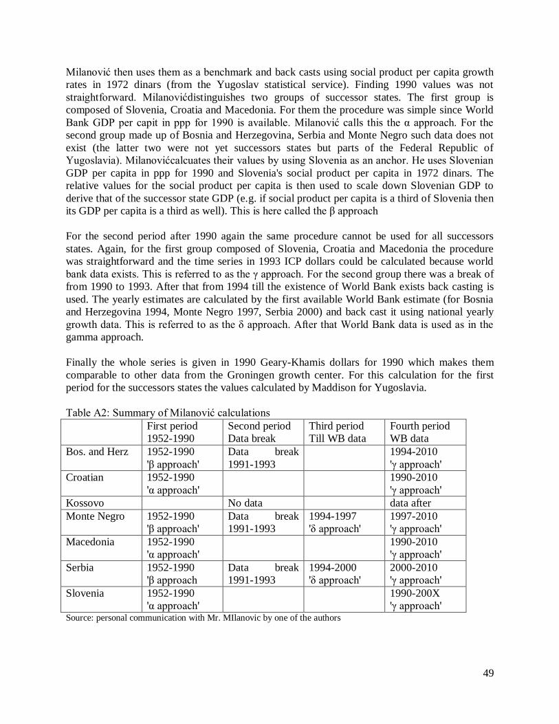
49
Milanović then uses them as a benchmark and back casts using social product per capita growth
rates in 1972 dinars (from the Yugoslav statistical service). Finding 1990 values was not
straightforward. Milanovićdistinguishes two groups of successor states. The first group is
composed of Slovenia, Croatia and Macedonia. For them the procedure was simple since World
Bank GDP per capit in ppp for 1990 is available. Milanović calls this the α approach. For the
second group made up of Bosnia and Herzegovina, Serbia and Monte Negro such data does not
exist (the latter two were not yet successors states but parts of the Federal Republic of
Yugoslavia). Milanovićcalcuates their values by using Slovenia as an anchor. He uses Slovenian
GDP per capita in ppp for 1990 and Slovenia's social product per capita in 1972 dinars. The
relative values for the social product per capita is then used to scale down Slovenian GDP to
derive that of the successor state GDP (e.g. if social product per capita is a third of Slovenia then
its GDP per capita is a third as well). This is here called the β approach
For the second period after 1990 again the same procedure cannot be used for all successors
states. Again, for the first group composed of Slovenia, Croatia and Macedonia the procedure
was straightforward and the time series in 1993 ICP dollars could be calculated because world
bank data exists. This is referred to as the γ approach. For the second group there was a break of
from 1990 to 1993. After that from 1994 till the existence of World Bank exists back casting is
used. The yearly estimates are calculated by the first available World Bank estimate (for Bosnia
and Herzegovina 1994, Monte Negro 1997, Serbia 2000) and back cast it using national yearly
growth data. This is referred to as the δ approach. After that World Bank data is used as in the
gamma approach.
Finally the whole series is given in 1990 Geary-Khamis dollars for 1990 which makes them
comparable to other data from the Groningen growth center. For this calculation for the first
period for the successors states the values calculated by Maddison for Yugoslavia.
Table A2: Summary of Milanović calculations
First period
1952-1990
Second period
Data break
Third period
Till WB data
Fourth period
WB data
Bos. and Herz 1952-1990
'β approach'
Data break
1991-1993
1994-2010
'γ approach'
Croatian 1952-1990
'α approach'
1990-2010
'γ approach'
Kossovo No data data after
Monte Negro 1952-1990
'β approach'
Data break
1991-1993
1994-1997
'δ approach'
1997-2010
'γ approach'
Macedonia 1952-1990
'α approach'
1990-2010
'γ approach'
Serbia 1952-1990
'β approach
Data break
1991-1993
1994-2000
'δ approach'
2000-2010
'γ approach'
Slovenia 1952-1990
'α approach'
1990-200X
'γ approach' Source: personal communication with Mr. MIlanovic by one of the authors

50
Milanović compares his estimates with three other sources, Maddison values for 2008, World
Bank values for 2008 and Eurostat values for 2007 tpo determine the reliability of his data.
Figure A1: Groningen (Milanović) growth project estimates for GDP per capita for successors
states in 1990 international dollars
0
5.000
10.000
15.000
20.000
19
52
19
57
19
62
19
67
19
72
19
77
19
82
19
87
19
92
19
97
20
02
20
07
Bosnia
Croatia
Macedonia
Slovenia
Montenegro
Serbia
Source: authors
A1.6 Constructing the time series data for this paper
When preparing the time series from 1952 to 2013 it would have been simplest to extend the
Gronningen/Milanović data. However the authors noticed a major inconsistency easily visible
from eyeballing the data presented in Picture A1. In Groningen data compiled by
BrankoMilanović in the fifties imply Macedonian GDP per capita is the third highest among the
Yugoslav republics and later successors states. This makes it higher than Serbian and
Montenegrin. This is obviously wrong and all primary indirect development data supports this
(literacy, social product per capita, economic structure, etc. data). If the data for Macedonia and
Serbia are questionable then the reliability for other successor states is lacks reliability.
As a result the authors decided to compose a new data set which avoids the inconsistences. The
calculation was made in the following way. One procedure was used for the data before 1990
and another to fill in the gap from 1990 to 1995 and after 1995 official GDP data was available.
The procedure was to apply the β approach to all successor states for the first period from 1952
to 1990. This means that for Slovenia, Croatia and Macedonia the α approach was replaced by
the β approach.
The pre 1990 GDP per capita calculated by assuming the World Bank number for Slovenia was
correct and used as the corner stone of the recalculation. This differs from the
Groningen/Milanović approach since the World Bank data for other successor states are not
used. The assumption about Slovenna data seems justified because as the most developed
successors state Slovenia had the best developed statistical service thus providing the most sound
base for the World Bank estimate. Also, it did not experience a long war and much material
damage (the Slovenian episode of Wars of the Yugoslav succession lasted 10 days, from June
26th to July 5th 1991 with less than half a dozen casualties altogether and no damages). The
51
GDP per capita for the other successor states was derived from Slovenian data and relative social
product per capita of the other successors states. For this the data from Yugoslav Statistical
Yearbook for 1990 was used, this is the last statistical yearbook complied by the Yugoslav
(federal) statisticians and thus it can be assumed the data is comparable. The GDP per capita for
a successor states was downscaled in the same proportion as was the social product per capita
smaller than the Slovenian one. The thus derived GDP per capita for every successors states was
then back casted using the social product growth rates for individual years. Yugoslav data allow
for back casting for todays territory of Serbia (i.e. without Kosovo and Monte Negro which both
were part of the rump Yugoslavia but eventually became successor states). In this way the time
series for Yugoslavia and its successor states was calculated for the 'socialist' period from 1952
to 1990.
The procedure is based on three assumptions, first that Slovenian data for 1990 is correct, second
that the relative values of GDP per capita and social product per capita are the same and third,
that yearly rates of growth of GDP and social product are the same. Only the second assumption
was checked with two other data sources, the WIIW data and Milenković (1991) and the
differences were not such as to justify mixing two data sets. There is another justification for the
procedure. One could assume that the deviations of social product and GDP per capita depend on
the level of development and should be larger for Slovenia that Kosovo since the former has a
larger share of services omitted by social product. However, the most reliable GDP per capita
data is the one compiled by Milenković (1991) as part of a UN sponsored project and he
concludes that because of direct aid to the less developed regions the difference of the two
variables does no depend on the level of development.
In comparison to the Groningen data it follows the same back casting procedure but uses
different benchmark value. The procedure avoids the most important deficiency of the
Groningen approach regarding the relationship of Macedonian and Serbian data. This can be
seen in Picure A2. Furthermore, the relative values in 1990 are based on primary data.
For the period from 1990 till 1995 for which GDP primary data from national statistical offices
using UNSNA data does not exist a different procedure was used. The 1995 World bank data for
every successors stares was assumed as correct.
For the analysis of the paper a time series from 1950 to 2015 had to be reconstructed for
Yugoslavia and the 7 successors states. Separate national estimates do exist for some of these
countries but the authors choose to use data compiled by BrankoMilanović and published under
the authority of a reputable source such a Angus Maddison and Groningen Growth Centre.
Figure A2: Time series for GDP per capita 1952-2015 in 1990 international dollars

52
Source: authors
0
2000
4000
6000
8000
10000
12000
14000
16000
18000
20000
19
52
19
54
19
56
19
58
19
60
19
62
19
64
19
66
19
68
19
70
19
72
19
74
19
76
19
78
19
80
19
82
19
84
19
86
19
88
19
90
19
92
19
94
19
96
19
98
20
00
20
02
20
04
20
06
20
08
20
10
20
12
Bosnia Croatia Macedonia Slovenia Montenegro Serbia

53
Appendix 2: The methodological approach to determining one or mutliple
break points
Economists often want to know whether there are points of discontinuity, i.e. structural breaks, in
the time series data they use. Frequently these points are chosen ad hoc, either through a
narrative approach, by identifying some characteristic of the series not covered in the data itself
(e.g. some institutional changes or exogenous shock) or by 'eye balling' the data. Neither is
precise and is subject to the whims of the researcher. To avoid this arbitrariness in determining
the date of structural change econometricians have designed tests that determine structural breaks
generated by the data itself. Two tests are now used.
The first one is the Quandt-Andrews test which can identify only one break point. This test is
briefly described in section A2.1. This test estimates the existence and timing of one structural
change. Later econometricians developed the Bai-Perron test which is a technique that permits
the estimation of multiple break points in the time series. The main features of the Bai-Perron
test used in this paper is described in section A2.2.
A2.1 The Quandt-Andrews test for one break point
The Quandt-Andrews test performs a Chow test for structural stability (Chow, 1960) between
every observation in the sample with the exception of a ‘trimming’ percentage of the sample.
Usually 7.5% in the first part and 7.5% in the last part of the sample, i.e. 15%, is trimmed. The
trimmed part is used to fit the equation but is not considered as a possible break date.
The Chow test testing procedure splits the sample in two parts and fits the underlying regression
in each subsample. Then classic F-statistic is computed, testing the equality of both parameters:
(A2.1.)
knn
SSRSSRk
SSRSSRSSR
Fnn
nnn
2
)(
21
21
21
In the equation SSRis the sum of squared residuals, n the whole sample, 1n and 2n are the size of
the two sub-samples and k is the number of parameters estimated in the equation.
Performing a Chow test requires choosing a priori breakpoint date. As a result, different
researchers pick different dates and can have completely different conclusions. The solution for
this ambiguity is to treat the break date as unknown. Quandt–Andrews breakpoint test resolves
this arbitrariness of the Chow test by performing a Chow test sequentially between every
observation in the sample. The critical values for the test form a non-standard distribution and
are higher than F and 2 critical values (Hansen, 2001). The p-values for the test are reported in
Hansen (1997). The drawback is that it detects only one breakpoint because it uses the maximum
F-statistic of all the performed F-tests, as suggested by Quandt (1960).
54
A2.2 The Bai-Perron test for multiple break points
Bai-Perron (1998) provides a framework for estimating multiple structural changes with an
ordinary least squares model (OLS) in time series data. The authors propose a sup Wald type test
with a null hypothesis of no change against an alternative which consists of an arbitrary chosen
number of break dates. Also, they provide an additional test that allows the null hypothesis of l
changes versus the alternative hypothesis of l+1changes. Bai-Perron (1998 and 2002) use these
two tests to form a specific to general modeling strategy which allows consistent estimation of
the appropriate number of changes in the series.
In this paper we chose to test for structural change in multiple series by using a common AR
formulation for all the series (similar to e.g. Stock and Watson (2004)). Additionally we control
for serial correlation and heteroscedasticity and test for multiple breakpoints in the parameters and . The equation we use is and on which they apply the Bai-Perron (1998) procedure is:
(A2.2) ititit yLy )(
wherey is the series of interest, i represents the specific country, t time, represents the
(possibly changing) mean of a series, L is the lag operator and the appropriate autoregressive
coefficient. This procedure differs from Stock & Watson (2003) as they test for one structural
change in the parameters and in the variance. The proposed equation and Bai &Perron specific to
general modeling constitute a common framework in dating multiple points of discontinuity
through multiple series and countries. The above presented methodology enables us to formally
test for structural change in various series, such as GDP.
However, the Bai-Perron tests for structural breaks use asymptotical critical values which guide
the choice of the date and number of structural breaks. These asymptotical critical values are
calculated for white Gaussian noise processes with a large number of observations. Although we
are dealing with a time span of over 60 years, the observations are yearly, so they do not
constitute a particularly large sample. Antoshin, Berg and Souto (2008) show that Bai-Perron
tests lack power when used in small samples. We approach the issue in two ways. First,
following Jones and Olken (2008) we may accept the shortcomings of the Bai-Perron tests and
state that the breakpoint identified by the Bai-Perron methodology are a subset of the bigger set
of “true” breakpoints. Secondly, in the results section we show that reasonable sample
manipulation may yield additional breakpoints.

55
Appendix 3: Convergence
The two approaches to convergence used in the paper are defined in greater detail below. The
first has been called the ‘classical approach’ and the second the ‘time series’ approach. Both are
standards in the literature so here already derived and tested equations are used.
A3.1 Classical approach 1: absolute β-convergence (unconditional β-convergence)
The classical approach to the analysis of convergence is derived from the predictions of the
Neoclassical one sector growth model (the Solow model). This model predicts that over time all
economies converge to the same equilibrium long term growth path, hence its name ‘absolute
convergence’. This is possible only if less developed economies have higher growth rates than
developing ones. This is the proposition tested by the absolute β-convergence (unconditional β-
convergence). The proposition has been tested frequently and the now standard formulation is
presented in Sala-i-Martin (1996). This approach is used here.
The absolute β-convergence (unconditional β-convergence) proposition is tested by equation
A2.1.
A3.1
In the equation denotes country i’s annualized real growth rate of GDP
between time t and t+T, and denotes the logarithm of country i’s real GDP per capita in
period t, while is an error term.
By testing the equation we can obtain the value of the coefficient on which we can base our
conclusion about income convergence among the selected countries. If <0 the slope is falling
and economies with higher incomes have smaller growth rates so there is absolute -
convergence, i.e. that countries with lover initial level of income in period t experience higher
average growth rate between period t and t+Tthan countries with higher initial level of income. If
0 then there is no absolute convergence.
A3.2 Classical approach 2: σ-convergence
Another measure of convergence called σ-convergence. If over time the difference among the
developed and less developed decreases then growth rates must become more similar and when
convergence is complete all economies grow at the same growth rate. This implies a re4duction
in the dispersion of growth rates. A good measure of dispersion is the standard deviation usually
denoted by σ and hence this measure of convergence is called σ-convergence
Following this line of reasoning -convergence can be defined as follows: group of countries
are converging in the sense of -convergence if the dispersion of their real per capita GDP
levels tends to decrease over time. Formally, we can write this condition as:

56
,where is the time t standard deviation of across countries.
A3.3 Pair convergence: time series approach
The previous two concepts of convergence, namely absolute β-convergence and σ-convergence,
measure convergence for any number of economies. Another approach to convergence looks at
the convergence of only two economies. The test for convergence between pair of the countries
used in this paper was derived by Bernard and Durlauf (1996). Contrary to the classical
approach, e.g. (Sala-i-Martin, 1996), Bernard and Durlauf (as well as Estrin and Uraga, 1997)
focus on the characteristics of time series. They define convergence through the equation A 2.2
A3. 2
This definition of convergence asks whether the long-run forecasts of output differences tend to
some steady state level as the forecasting horizon tends to infinity. If is a finite
mean stationary process then by this definition of convergence the conditions for convergence
are be satisfied. This definition has natural testable analogy from the unit root/cointegration
literature. In order for countries i and j to converge their outputs must be cointegrated with
cointegrating vector [1, -1].
The formal econometrical analysis of the above definition is based on the equation A 2.3 of the
augmented unit root test (ADF)
A3. 3
Where the variable is the logarithmic difference in per capita output between economies i and
j in the period t , T is a deterministic trend and g is the maximum number of time lags
which is sufficient for to represent IID process with , distribution.
In the equation is stationary process if , meaning that the income difference between
two economies is constant and stable, i.e. that the economies are following the same growth
trajectory, on different levels of income. If the process is not stationary we analyze graphical
representation of time series to determine whether countries are converging to or diverging from
its pair countries.