The Virtual Aquarium: Simulations of Fish Swimming · The Virtual Aquarium: Simulations of Fish...
15
The Virtual Aquarium: Simulations of Fish Swimming M. Curatolo, L. Teresi Comsol Europe Conference, Grenoble, France October, 14 ~ 16, 2015 Università Roma Tre, Italy
Transcript of The Virtual Aquarium: Simulations of Fish Swimming · The Virtual Aquarium: Simulations of Fish...
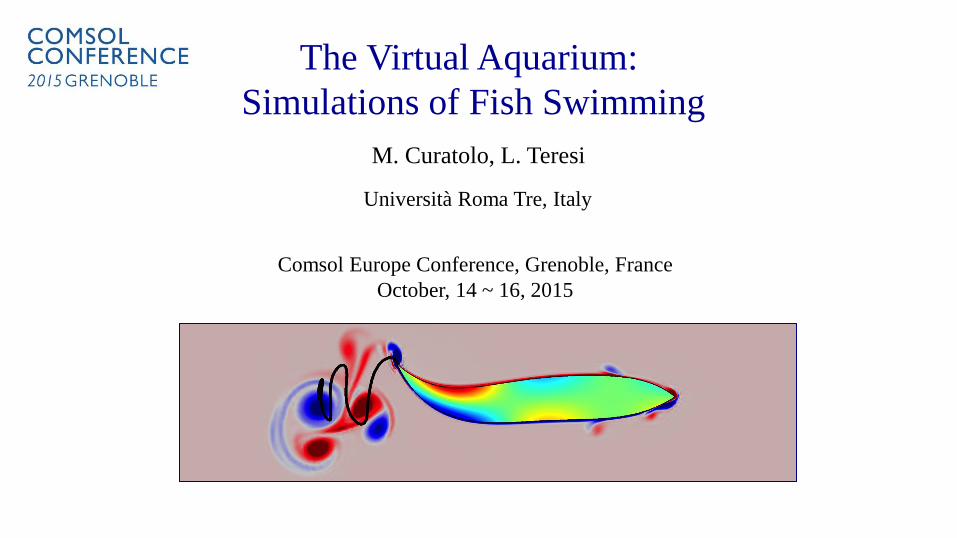
The Virtual Aquarium:
Simulations of Fish Swimming
M. Curatolo, L. Teresi
Comsol Europe Conference, Grenoble, France
October, 14 ~ 16, 2015
Università Roma Tre, Italy
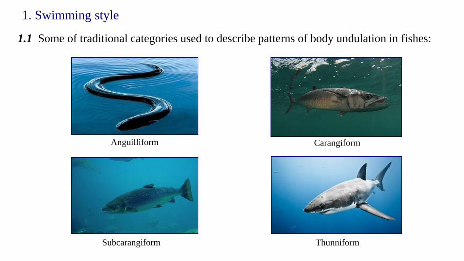
1. Swimming style
Anguilliform
Subcarangiform
Carangiform
Thunniform
1.1 Some of traditional categories used to describe patterns of body undulation in fishes:
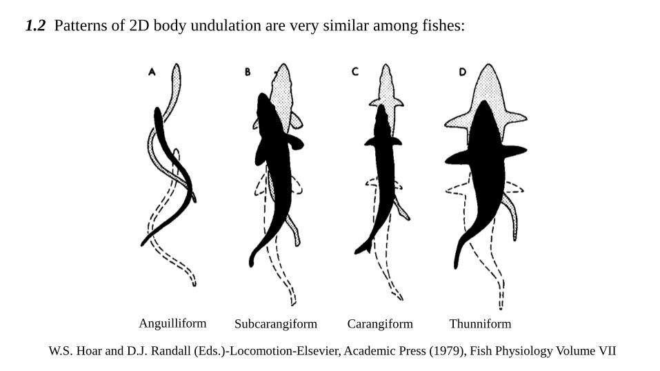
1.2 Patterns of 2D body undulation are very similar among fishes:
Anguilliform Subcarangiform Carangiform Thunniform
W.S. Hoar and D.J. Randall (Eds.)-Locomotion-Elsevier, Academic Press (1979), Fish Physiology Volume VII
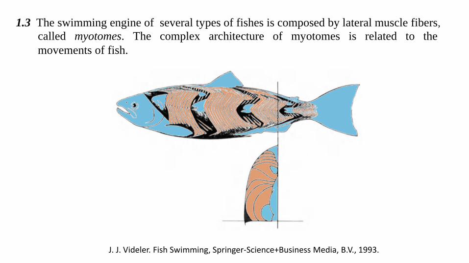
1.3 The swimming engine of several types of fishes is composed by lateral muscle fibers,
called myotomes. The complex architecture of myotomes is related to the
movements of fish.
J. J. Videler. Fish Swimming, Springer-Science+Business Media, B.V., 1993.
J. J. Videler. Fish Swimming, Springer-Science+Business Media, B.V., 1993.
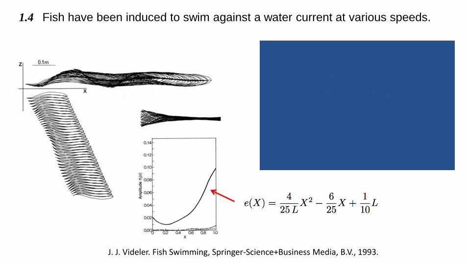
1.4 Fish have been induced to swim against a water current at various speeds.

1.5 Carangiform swimming style shows a traveling wave along the body;
viscosity. System (1) is supplemented with bound-
ary and init ial condit ions. In our case, the solid
represents a fish-like body which is surrounded by
fluid; we call @⌦sf the interface between the fish
and the fluid, and we pose FSI condit ions on such
interface:
S ns = Γ n f , v f = u̇s , on @⌦sf ⇥T . , (2)
with ns normal to the solid boundary and n f nor-
mal to the fluid boundary; @⌦f represents the
boundary of the aquarium on which we assign a
no-slip wall condit ion for the fluid:
v f = 0 in @⌦f ⇥T . (3)
Finally, we assign homogeneous init ial condit ions.
The fluid is assumed to be incompressible and
linearly viscous; its st ress Γ is given by:
Γ = − pI + 2µf (sym r v f ) −2
3µf (div v f ) I , (4)
where p is the fluid pressure. The solid is assumed
to be isot ropic and linear elast ic; its st ress S is
given by:
S = 2µs Ee + λ t r (Ee) I , (5)
with µs, λ the Lame’s moduli, Ee = E − Eo the
elast ic st rain; E is the non-linear st rain, measure:
E = sym r us +1
2r uT
s r us , (6)
and Eo the distort ions field (aka, pre-st rains).
The muscle act ions are modeled by a t ime-
evolving distort ion field Eo = Eo(X , Y, t) that pro-
duces the sought flexural mot ion of the fish-like
body. Within this approach, a muscle generates
mot ion, possibly without st ress; as example, if the
imposed distort ion is compat ible, that is, if a dis-
placement us, such that sym r us = Eo, can be
realized. In our case, the lateral mot ion of the
fish is reacted upon by the force exerted by the
surrounding fluid, and any muscles act ion is ac-
companied by st ress product ion.
Weset our problem in 2D; the referenceconfigu-
rat ion of the fish-like body is a st reamlined region
of the X Y plane, whose symmetry axis lies in the
X-axis; tail and head are at (0, 0) and (L, 0), re-
spect ively. The contour Y = c(X ) is given by a
mirrored 5t h order polynomial funct ion:
Y = c(X ) = a1 X 5 + a2 X 4 + a3 X 3 + a4 X 2 + a5 X .
(7)
with
a1 = − 10.55ts
L 5, a2 = 21.87
ts
L 4, a3 = − 15.73
ts
L 3,
a4 = 3.19ts
L 2, a5 = 1.22
ts
L,
where ts is the maximum fish thickness and L in-
dicates the fish length [4]; the result ing reference
configurat ion is shown in Fig.(1).
Denot ing with Y= h(X,t ) the t ransversal dis-
placement of the axis, the relat ion between distor-
t ion Eo and the curvature of the axis − @2 h/ @X 2
reads as:
Eox x (X , Y, t) = − Y
@2h(X , t)
@X 2. (8)
To define a swimming style, we first assign the
funct ion h(X , t), and then derive the muscle-
driven distort ions Eox x by integrat ing (8) twice.
X
Ymax thickness
X = L
c(X )
fish axis
Figure 1: Reference shape of the fish-like body; the con-
tours ± c(X ) are paramet rized by eq. 7.
Figure 2: Shape of the fish axis at di↵erent t imes; ampli-
t ude of movements is much larger at t he tail (left ) t han
at the head (right ), and is enclosed in the envelopes. I t is
present an amplit ude wave moving towards the tail, see the
posit ion of amplit ude maximum at t imes t1 < t2 < . . . <
t6 ; fish mot ion is rightward.
We use as benchmark swimming-style the
carangiform style; the t ransversal displacement of
2
Envelope
J. J. Videler. Fish Swimming, Springer-Science+Business Media, B.V., 1993.
Traveling-wave Time
switch
Wave number
Angular frequency
Activation time
Wave velocity:
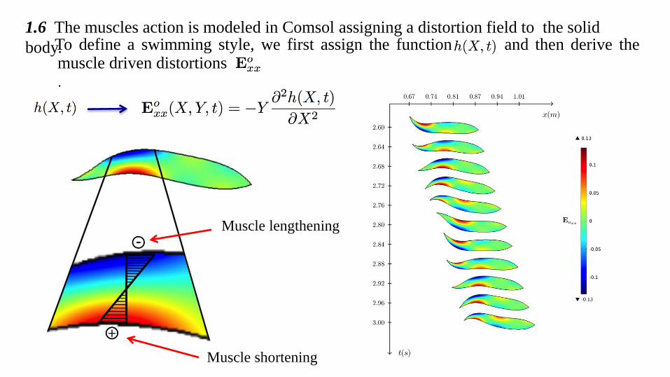
1.6 The muscles action is modeled in Comsol assigning a distortion field to the solid
body. To define a swimming style, we first assign the function and then derive the muscle driven distortions m .
Muscle shortening
Muscle lengthening
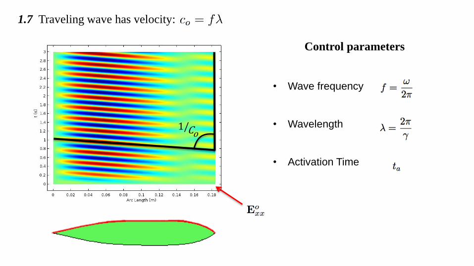
1.7 Traveling wave has velocity: :
1/ C o
Control parameters
• Wave frequency
• Wavelength
• Activation Time
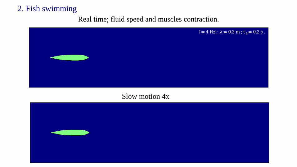
2. Fish swimming
Real time; fluid speed and muscles contraction.
Slow motion 4x
f = 4 Hz ; λ = 0.2 m ; t = 0.2 s . a
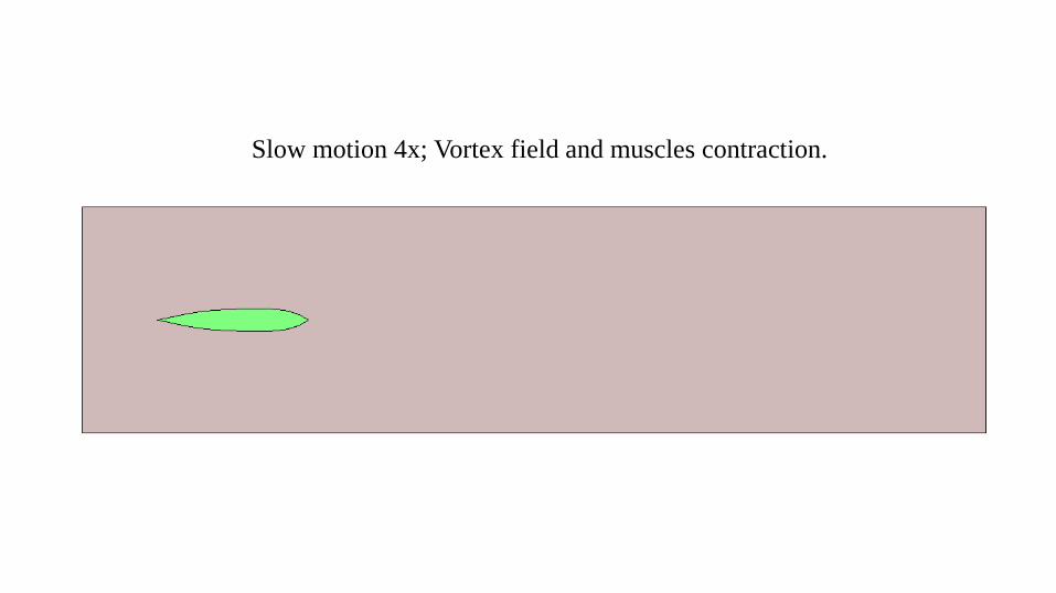
Slow motion 4x; Vortex field and muscles contraction.

2.1 Vortices are released at the end of every stroke.
Mutual distances between vortices do not change:
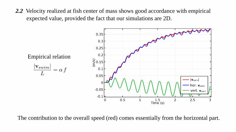
2.2 Velocity realized at fish center of mass shows good accordance with empirical
The contribution to the overall speed (red) comes essentially from the horizontal part.
expected value, provided the fact that our simulations are 2D.
Empirical relation
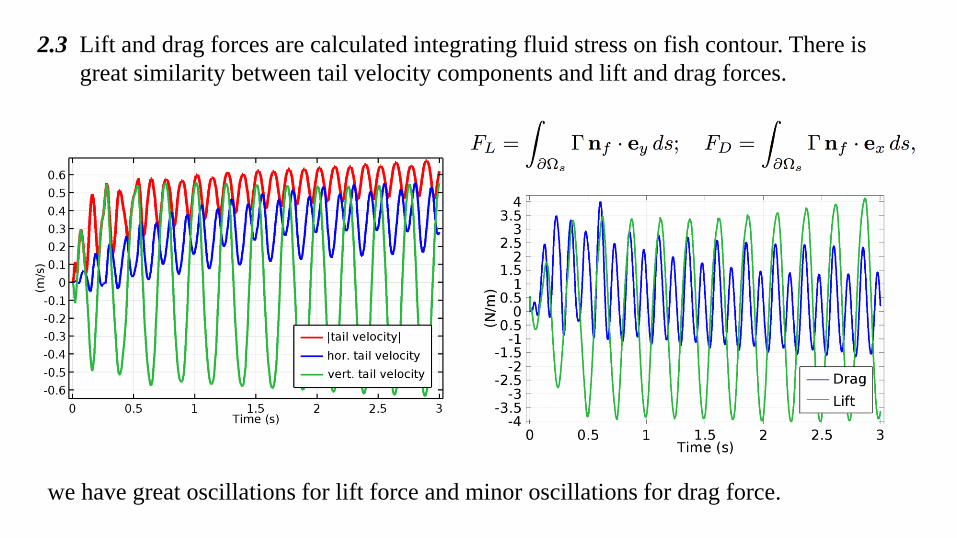
2.3 Lift and drag forces are calculated integrating fluid stress on fish contour. There is
we have great oscillations for lift force and minor oscillations for drag force.
great similarity between tail velocity components and lift and drag forces.
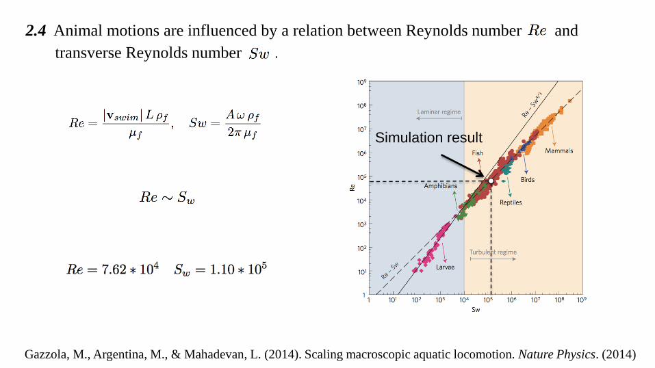
2.4 Animal motions are influenced by a relation between Reynolds number and
Gazzola, M., Argentina, M., & Mahadevan, L. (2014). Scaling macroscopic aquatic locomotion. Nature Physics. (2014)
transverse Reynolds number .
Simulation result
3. Comsol settings
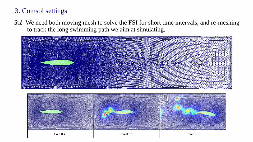
3.1 We need both moving mesh to solve the FSI for short time intervals, and re-meshing to track the long swimming path we aim at simulating.


![[eBook] - Aquarium - The Reef Aquarium - Vol.1](https://static.fdocuments.in/doc/165x107/55cf988e550346d033984c0f/ebook-aquarium-the-reef-aquarium-vol1.jpg)