The Use of Long-Run Restrictions for theIdentification of Technology ShocksNeville R. Francis, Michael T. Owyang, and Athena T. Theodorou

NOVEMBER/DECEMBER 2003 53

I n many economic models, business cyclesare driven by some combination of monetary,fiscal, and technological innovations, where

“technology” is often thought of as the unexplain-able component of the business cycle that is mani-fested as a change in the overall productive capacityof the economy. Recently, a growing empirical litera-ture has undertaken the challenge of defining tech-nology shocks and their effects on the economyin structural statistical models.

In this paper, we survey the recent literature onlong-run identified technology shocks. We presentthe results of a bivariate vector autoregression (VAR)with labor productivity and labor hours as a bench-mark for the recent results found for technologyshocks. We then propose an alternative approachfor identifying and studying the effects of technologyshocks.

We propose a reverse approach to that used inthe structural VAR literature, the motivation of whichis to provide a robustness check of the recent resultsfrom the existing literature. Our new methodologyentails four basic steps. We first estimate the reduced-form VAR, saving the coefficient and the error variance-covariance matrices. Given the estimatedreduced-form coefficient and covariance matrices,the second step is to constrain the impulse responsefor labor productivity. Specifically, we restrict thesign of the impulse response for productivity suchthat technology shocks have long-lasting positiveeffects on productivity. The third step is to collectall the shocks that can generate this long-horizonresponse of productivity—we call these disturbancespotential technology shocks. The final step is toexamine the response of labor hours to these shocks.Contrary to standard real business cycle (RBC) theory,recent studies in this literature have found that laborhours respond negatively to a positive technologyshock. We test the robustness of this result.

The remainder of the paper is organized as follows: We define the properties of the VAR-basedtechnology shock and review the current empiricalfindings in the second section. In the third section,we examine a standard application of long-runrestrictions used to identify technology shocks andpresent our (bivariate) benchmark results from thisexercise. In the fourth section, we employ an alter-native form of a long-run restriction that is adaptedfrom the agnostic algorithm originally proposed byUhlig (1999).

EMPIRICAL TECHNOLOGY SHOCKS:A SURVEY

The traditional view in macroeconomics wasthat economic fluctuations arose from transitoryshocks, e.g., temporary shocks to monetary andfiscal policy. Secular trends were believed not tocontribute to quarter-to-quarter or even year-to-yearfluctuations in macroeconomic data. In a very influ-ential paper, King et al. (1991) empirically examinedthe effects of shifts in stochastic trends common toseveral macroeconomic series. They presented aneconomic model with a single common stochastictrend, interpreted as a permanent shock to produc-tivity, that altered the steady state of the modeleconomy. This stochastic trend, the unit root inproductivity, is now widely referred to as a “tech-nology shock”; currently, the challenge for macro-economists is how to more accurately identify thismeasure of technology shocks.

The growth accounting approach proposed bySolow (1957) has been widely used to identify tech-nology shocks. Under the assumption of competitivemarkets and constant returns to scale in production,total factor productivity (or the Solow residual) isthat part of output that is left unexplained afteraccounting for the contributions of capital and labor.A typical growth accounting equation would be ofthe form:

,

where Yt is period-t output; Kt and Lt are period-tcapital and labor, respectively; γ is the labor shareof output; and At is the so-called Solow residual.

log( ) log( ) ( )log( ) log( )Y L K At t t t= + − +γ γ1Neville R. Francis is an assistant professor of economics at LehighUniversity; Michael T. Owyang is an economist and Athena T. Theodorouis a research associate at the Federal Reserve Bank of St. Louis. Theauthors thank Valerie Ramey and Tara Sinclair for valuable comments.Kristie Engemann and Mark L. Opitz provided research assistance.

© 2003, The Federal Reserve Bank of St. Louis.

Innovations to the Solow residual were thoughtof as shocks to technology.1 However, there are threepotential shortcomings with the use of the Solowresidual as a proxy for technology shocks. First,growth accounting does not incorporate eitherworkers’ effort or capital utilization. Thus, embeddedin the residual At are these confounding measuresthat have nothing to do with technology shocks.Second, the probability of technological regressusing the Solow residual is of the order of 40 per-cent, which is implausible to some economists. It isnot apparent that the structural VAR (SVAR) methodovercomes this criticism, implying that it is nearlyequally likely to have technological regress asprogress. Third, the measure failed what are nowreferred to as the Hall (1988) and Evans (1992)tests. These studies found that the Solow residualis correlated with other exogenous shocks—suchas shocks to money, interest rates, and governmentspending—that are not related to technology.2

These shortcomings led economists either toseek to improve upon the Solow residual or searchfor an alternative measure of technology shocks.Basu, Fernald, and Kimball (1998) sought to improveupon the Solow residual by incorporating unob-served factor inputs into their estimations. Theyfollowed Hall (1990) and regressed the growth rateof output on the growth rate of inputs at a disaggre-gated level with proxies for capacity utilization.Technological change is then defined as an appro-priately weighted sum of the resulting residuals.They found that technological improvements con-tradict RBC theory predictions about the (technology-driven) co-movement of labor hours and productivityacross the business cycle; specifically, hours fall, atleast in the short run, when hit with a productivity-improving technology shock.

The search for an alternative measure of tech-nology shocks has proceeded along two lines. Thefirst line of research concerns the assumption(s) usedto identify technology shocks. The second lineinvolves the choice of data used to identify technol-ogy shocks and asks: Are technology shocks either(i) a manifestation of the unexplained component

of labor productivity or output or (ii) the culminationof research and development?

Proceeding along the first line of research, Gali(1999) attempted to disentangle technology and non-technology shocks by analyzing labor productivityand hours of employment. He estimated a SVARwith the key identifying assumption that technologyshocks alone can produce long-run effects on laborproductivity.3 Gali estimated a bivariate model ofproductivity and hours.4 He found that hours fell inresponse to a shock that permanently raised laborproductivity (the technology shock). Gali thus con-cluded that technology shocks were not the drivingforce behind cyclical fluctuations and that his “non-technology” shocks better explained the short-runmovements in aggregate economic data. Kiley (1998)followed Gali and applied a similar methodology to17 two-digit manufacturing industries. He foundthat, for a majority of these industries, technologyshocks identified by these SVARs produced the samenegative hours response as found for the aggregatedata.

Francis and Ramey (2002) used Gali as a startingpoint in their recent analysis of technology shocks.Using the SVAR approach, they reexamined Gali’swork by first testing whether the shocks identifiedin this framework can be plausibly interpreted astechnology shocks. They first derived additionallong-run restrictions and used them as overidentify-ing tests. For example, they estimated a model ofreal wages and hours with the assumption that onlytechnology shocks can have permanent effects onreal wages. If this assumption is true, then real wagesand productivity should share a common trend, anassumption not rejected by the data.5 Next, theyaugmented Gali’s basic model with data on realwages, investment, and consumption and deter-mined whether the impulse responses for thesevariables accorded with theory. Finally, they testedwhether their technology shocks were Granger-caused by exogenous events unrelated to technologyas per Hall (1988) and Evans (1992). Their measureof technology survived the scrutiny of all three tests.

54 NOVEMBER/DECEMBER 2003

3 In a bivariate framework, the employed identification is equivalentto a Wold causal chain structure in the long run.

4 Gali (1999) also estimates a five-variable model that includes money,inflation, and interest rates. Results from this model are consistentwith the bivariate framework.

5 The first-order condition states that workers are each paid theirmarginal product. Therefore, it stands to reason that the same assump-tion for the effect of technology shocks on labor productivity mustalso hold for technology shocks on real wages.

Francis, Owyang, Theodorou R E V I E W

1 This view is not the consensus of the growth accounting literature.For example, Denison (1979) views productivity as a measure ofsociety’s ability to increase standards of living.

2 King and Rebelo (1999) provide a comprehensive survey of the RBCliterature. In particular they highlight the features of the RBC model,e.g., indivisible labor and capital utilization, that generate business-cycle-like second moments while correcting for the failures of theSolow residual.

However, they still found that labor hours respondednegatively on impact to a technology shock.6

Shea (1999) proceeded along the second line ofresearch. He used data on both patents and researchand development to identify technology shocksand found that hours fell in response to a technologyshock. However, unlike the above studies, the declinein hours is a long-run response—that is, hours risein the short run but then eventually fall.

In sum, using different methodologies to identifytechnology shocks, these recent lines of researchhave produced similar results. Further, the identifiedtechnology shock is unable to explain a substantialproportion of the variation in hours across thebusiness cycle. Our contribution will be to add afourth methodology that provides a robustnesscheck of the SVAR results.

IMPLEMENTING LONG-RUN RESTRICTIONS

In this section, we present a bivariate long-runrestricted SVAR model of productivity and hours asa benchmark to the technology literature. Essentially,this section reproduces the bivariate results describedin Gali (1999) and Francis and Ramey (2002).

Data

The data are quarterly and cover the period1948:Q1 to 2000:Q4. The labor productivity seriesis from the Bureau of Labor Statistics (BLS) “Indexof output per hour, business,” while the labor hoursseries is from the BLS “Index of hours in business.”We tested and failed to reject unit roots for both laborproductivity and hours; therefore, in our benchmarkVAR specification, we enter these series in first differ-ences. Productivity and labor are also not cointe-grated. We use four lags of the dependent variablesin each equation of the VAR. The lag length waschosen by means of the Schwarz or Bayesian infor-mation criterion (BIC).

Econometric Framework

The recent methodology of choice in the tech-nology shock literature is the SVAR, a standardreduced-form VAR with additional restrictions that

are drawn from theory to separate and identify thecomponents of the residuals. These restrictions canbe short run (often comprising short-run restrictionsor the impact effects of shocks) or long run. A dis-cussion of long-run restrictions follows.

Consider the following k-lag VAR:

Φ(L)Yt=ε t,

where

,

,

and Φ(L) is a kth-order matrix polynomial in the lagoperator. The VAR can be rewritten in its movingaverage (MA) representation:

(1) Yt=C(L)ε t,

where C(L) is a (infinite) polynomial matrix in thelag operator Φ(L)=C(L)–1. The series xt denotes thelog of labor productivity, and nt denotes the log oflabor hours. We label ε t

x the technology shock andε t

n the non-technology shock, and we make the usualassumption that these shocks are orthogonal andserially uncorrelated.

For ease of exposition, it is useful to rewrite (1) as

(2) .

We impose long-run restrictions to identify thetechnology shock, ε t

x. Each of the matrices in (2) isa polynomial in the lag operator. To achieve exactidentification, we restrict the non-technology shock’slong-run impact on productivity to be zero. Thisassumption identifying the technology shock impliesthat C12(1)=0, which restricts the unit root in pro-ductivity to originate solely from the technologyshock.7 The identifying restrictions do not restrictthe effect the technology shock can have on hoursat either the long or short horizon.8

We estimate the model using the method pro-

YC L C L

C L C Lttx

tn

=

11 12

21 22

( ) ( )

( ) ( )

ε

ε

εε

εttx

tn

=

Yx

ntt

t

=

∆∆

NOVEMBER/DECEMBER 2003 55

7 In principle, the model presented above could be augmented to mea-sure the effects of shocks on other variables (see Gali, 1999, and Francisand Ramey, 2002). The identification scheme here assumes that anyother shock, regardless of the size of the system, has no long-runeffect on labor productivity.

8 It can be shown that the identification scheme explained in this sectionis equivalent to a Wold causal chain on the steady-state structure ofthe model (see Rasche, 2001).

FEDERAL RESERVE BANK OF ST. LOUIS Francis, Owyang, Theodorou

6 Christiano, Eichenbaum, and Vigfusson (2003) and Uhlig (2002)challenge the results of the aforementioned literature. They claim thathours entered in levels would overturn the negative short-run hoursresponse when a technology shock hits the economy. However, Francisand Ramey (2003), in another unpublished manuscript, show thathours, properly detrended, experiences a decline on impact of atechnology shock.

posed by Shapiro and Watson (1988). By using thismethod we can estimate the equations in the VARone at a time. The productivity equation is as follows:

(3) ,

where ∆2 is the square of the difference operator.Imposing the long-run restriction is equivalent torestricting the hours variable to enter the produc-tivity equation (3) in double differences.9 Becausethe current value of ∆2nt will be correlated with ε t

x,we estimate this equation using instrumental vari-ables. We use lags 1 through p of ∆xt and ∆nt asinstruments. The hours equation is then estimatedas follows:

∆ ∆ ∆x x nt xx j t jj

p

xn jj

p

t j tx= ∑ + ∑ +−

= =

−

−α β ε, ,1 0

12

(4) .

Technology, ε tx, enters into the hours equation (4) in

order to achieve orthogonality between the tech-nology and non-technology shocks. We estimate thehours equation using ordinary least squares, sincethere is no contemporaneous independent variablethat would be correlated with the residual ε t

n. TheShapiro-Watson methodology, applied to the samedata, produces results identical to the matrix methodused by Gali.10 We present results from an illustrativetwo-variable system in the next subsection.

Benchmark Results

Figure 1 presents the impulse responses from ashock to technology in the bivariate model of labor

∆ ∆ ∆n x nt nx j t jj

p

nn jj

p

t j n x tx

tn= ∑ + ∑ + +−

= =−α α ρ ε ε, , ,

1 1

56 NOVEMBER/DECEMBER 2003

10 The interested reader is directed to Appendix A for a detailed derivationof the long-run restriction methodology. There, we demonstrate theequivalence between the matrix method and the Shapiro-Watsonmethod of long-run identification.

Francis, Owyang, Theodorou R E V I E W

Productivity

0.50

0.60

0.70

0.80

0.90

1.00

1.10

0 1 2 3 4 5 6 7 8 9 10 11 12Quarter

Labor Input

–0.80

–0.60

–0.40

–0.20

0.00

0.20

0.40

0 1 2 3 4 5 6 7 8 9 10 11 12Quarter

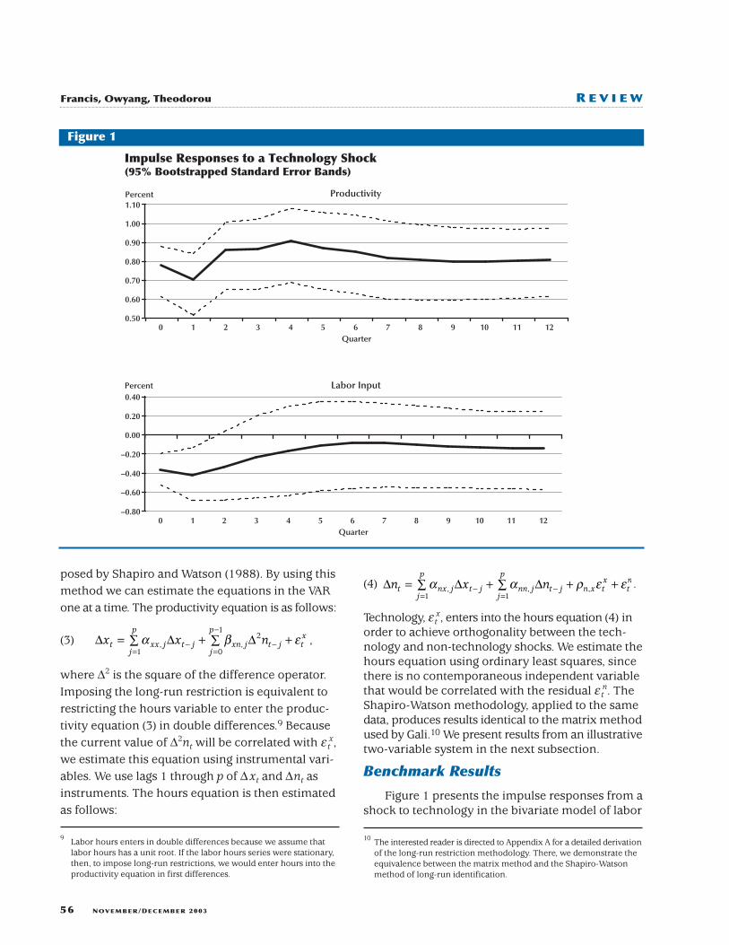
Impulse Responses to a Technology Shock(95% Bootstrapped Standard Error Bands)

Percent

Percent

Figure 1

9 Labor hours enters in double differences because we assume thatlabor hours has a unit root. If the labor hours series were stationary,then, to impose long-run restrictions, we would enter hours into theproductivity equation in first differences.

productivity and hours.11 Labor productivity immedi-ately rises by 0.8 percent, displays a hump-shapedpattern, and eventually settles to a new steady stateapproximately 0.8 percentage points above its pre-shock level. This persistent rise in productivity is atthe heart of the identification, as only the technologyshock can have this permanent positive effect.

The hours response is somewhat curious. Onimpact, labor hours experience a statistically signifi-cant decline in response to the technology shock;moreover, the point estimate for the responseremains negative for the entire response period.However, according to the 95 percent bootstrappedconfidence bands, the decline in labor hours is sta-

tistically significant for only two quarters; thereafter,it is insignificantly different from zero.

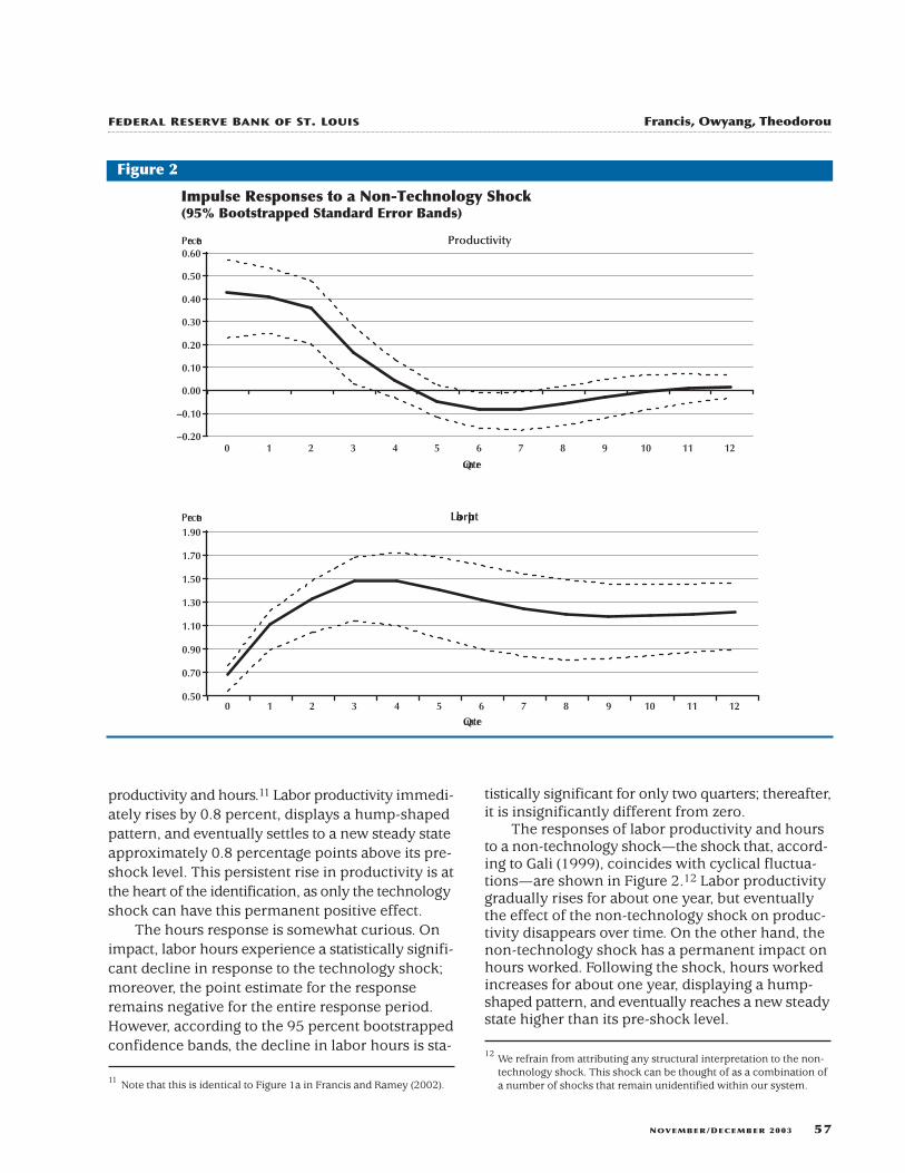
The responses of labor productivity and hoursto a non-technology shock—the shock that, accord-ing to Gali (1999), coincides with cyclical fluctua-tions—are shown in Figure 2.12 Labor productivitygradually rises for about one year, but eventuallythe effect of the non-technology shock on produc-tivity disappears over time. On the other hand, thenon-technology shock has a permanent impact onhours worked. Following the shock, hours workedincreases for about one year, displaying a hump-shaped pattern, and eventually reaches a new steadystate higher than its pre-shock level.

NOVEMBER/DECEMBER 2003 57

12 We refrain from attributing any structural interpretation to the non-technology shock. This shock can be thought of as a combination ofa number of shocks that remain unidentified within our system.

FEDERAL RESERVE BANK OF ST. LOUIS Francis, Owyang, Theodorou

Productivity

–0.20

–0.10

0.00

0.10

0.20

0.30

0.40

0.50

0.60

0 1 2 3 4 5 6 7 8 9 10 11 12

L abor Input

0.50

0.70

0.90

1.10

1.30

1.50

1.70

1.90

0 1 2 3 4 5 6 7 8 9 10 11 12

Percent

Percent

Quarter

Quarter

Impulse Responses to a Non-Technology Shock(95% Bootstrapped Standard Error Bands)

Figure 2

11 Note that this is identical to Figure 1a in Francis and Ramey (2002).

IMPULSE RESPONSE RESTRICTIONS

In this section, we demonstrate how long-runrestrictions can be implemented in a frameworkthat leaves the structural parameters of the VARunrestricted but, instead, imposes sign restrictionson the resulting impulse responses (see Uhlig,1999).13 We can, therefore, estimate the model with-out imposing the exact restrictions on the estimatedparameters, as in the long-run identification schemesof Blanchard and Quah (1989) and Shapiro andWatson (1988). We search for shocks that produceimpulse responses consistent with what we believetechnology should produce, i.e., a long-run positiveresponse to labor productivity. Our goal is to deter-mine the robustness of the results found in thepreceding section by determining the percentageof long-run effective shocks that produce an hours/productivity negative co-movement.

An additional advantage to this approach, whichwe leave to be exploited by further research, is thathypothetical responses can be posed. The resultingshocks required to induce those responses can becomputed and used to perform counterfactualexperiments. In this sense, we can work backwardto test the validity of our assumptions about theeffects of the shocks by performing, say, exogeneitytests.14

Framework

Here, we outline the methodology that incor-porates restrictions on the signs of the impulseresponses to identify the model. What we are doing,in essence, is defining how a type of shock shouldeffect the economy and determining which shocksmight generate those results. While, to the casualreader, this identification might seem to be con-structed backward, it has theoretical foundationsthat are detailed in Appendix B.

Formally, the reaction to the reduced-form shock(et from Appendix B) cannot be interpreted in astructural context. However, it can be shown thatthe structural shock εt is related to the reduced-form shock by means of the contemporaneousimpact matrix, A0:

et=A0–1εt,

where A0–1A0

–1′=Σ. Thus, the j th column of thematrix A0

–1 can be interpreted as the contempora-neous effect of the jth fundamental shock (which wewill call an impulse vector). However, this decompo-sition is not unique; for any orthonormal matrix Q,A0

–1QQ′A0–1′=Σ is also a permissible decomposition.

In the previous section, we distinguished betweenacceptable rotations by imposing restrictions on theform of the rotation matrix Q.

The identification technique we employ in thissection involves sampling from the distributions forboth the coefficient and covariance matrices thatare estimated from the model’s reduced form. Wedraw a candidate impulse vector and compute theimpulse response; each impulse vector that gener-ates an impulse response consistent with a prede-termined set of sign restrictions is saved.15 Iterationof this process generates a distribution for theimpulse vectors we will call technology shocks.

While the methodology utilized in the previoussection uniquely identified a (estimated) reduced-form shock, the technique in this section estimatesa distribution for this shock. Exact identificationusing this technique requires a large number ofrestrictions, since the constraints on the impulseresponses may not bind at all horizons. Thus, insteadof imposing, for example, an explicit causal ordering,we are able to define the technology shock basedon its ex post impulse response for certain variables.We concentrate on identification of the technologyshock. In principle, other shocks that are effect-orthogonal, i.e., have sets of mutually exclusiverestrictions, could also be identified.

A number of recent papers have employed thisalgorithm to impose sign restrictions on impulseresponses. Uhlig (1999, 2001) and Owyang (2002)restrict the responses of both inflation and interestrates to identify a monetary shock. Mountford andUhlig (2002) impose restrictions on revenues,expenditures, and deficits to identify fiscal shocks.However, these applications of the algorithm havecentered primarily on the short-run responses toshocks. Here, we can adapt the algorithm to test forrestrictions at long horizons. In this application, weconstrain the long-run response of labor productivityto a technology shock to be positive.16

58 NOVEMBER/DECEMBER 2003

15 Mathematical details for the estimation and identification can befound in Appendix C. For an explicit discussion of the relationshipbetween the impulse vector and the identified structural shock, seeUhlig (1999).

16 In addition to long-horizon restrictions on the productivity response,we also impose impact restrictions. We assume that a positive technol-ogy shock raises productivity on impact.

Francis, Owyang, Theodorou R E V I E W

13 Other ex post restrictions could also be employed. Examples of theseinclude restricting the forecast error variances (Faust, 1998) or thecross-correlation (Canova and De Nicolo, 2002).

14 An example of this line of research can be found in Francis and Owyang(2003).

Empirical Results

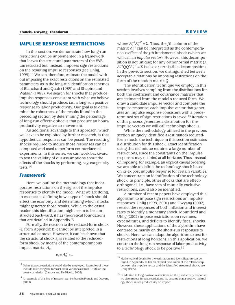
The system that we estimate is a VAR with priordistributions on the parameters that we describe inAppendix C. We make 1000 draws from the poste-rior distributions generated by estimating the VAR.For each draw from the parameter space, we draw1000 candidate shocks.17

The distributions of the impact effects on thetwo-system variables are shown in Figure 3. Weinclude the point estimates of the impact effectsfor the exactly identified shock from the previoussection. Labor productivity’s impact response fromthe SVAR lies to the right of the mean of the impact

NOVEMBER/DECEMBER 2003 59

of this shock can be achieved either through independent draws orby utilizing an orthogonality assumption to decompose the systemresiduals.

FEDERAL RESERVE BANK OF ST. LOUIS Francis, Owyang, Theodorou

Productivity

0

20

40

60

80

100

120

140

160

180

200

0.33 0.36 0.39 0.42 0.45 0.47 0.50 0.53 0.56 0.58 0.61 0.64 0.67 0.69 0.72 0.75 0.78 More

Labor Input

0

50

100

150

200

250

–0.56 –0.52 –0.47 –0.43 –0.39 –0.35 –0.30 –0.26 –0.22 –0.18 –0.13 –0.09 –0.05 –0.01 More

Frequency

Frequency

Distributions of the Impact Effects on the Two-System Variables

Hours impactresponse from SVAR

Productivity impactresponse from SVAR

Figure 3

17 We forgo identification of the hours shock in this section. Identification

distribution from the sign-restriction algorithm.That is, the initial productivity response from theSVAR is greater than the mean impact responseobtained from the sign-restriction algorithm. How-ever, the opposite is true for the hours response.That is, the hours response from the SVAR lies tothe left of the mean of the impact distribution fromthe sign-restriction approach. Therefore, the sign-restriction algorithm produces initial hours responsesthat are invariably less negative (i.e., closer to zero)than the impact response obtained from the SVARwith long-run restrictions. In this sense the sign-restriction approach is less restrictive than the SVARapproach but nevertheless produces an initial hoursresponse that is negative on average.18

The resulting mean impact effects of the iden-tified technology shock are

,

(0.62 for labor productivity and –0.31 for laborhours), and the associated impulse responses are

ˆ.

.a =

−

0 62

0 31

60 NOVEMBER/DECEMBER 2003

18 The same is true when the sign-restriction algorithm has hours enter-ing the VAR in levels. This means that the SVAR with hours in levelsdoes not impose enough restrictions to identify technology shocks.In these SVARs, non-technology shocks have long-lasting effects onproductivity, contrary to the initial identifying assumption. Ouralgorithm with hours in levels imposes enough ex post restrictionsto circumvent such problems and thus produces negative labor hoursresults just like its first-differenced counterpart. See Francis and Ramey(2003) for further exposition.

Francis, Owyang, Theodorou R E V I E W

Productivity

–0.20

0.00

0.20

0.40

0.60

0.80

1.00

1.20

1.40

1.60

1.80

1 3 5 7 9 11 13 15 17 19

Labor Input

–2.00

–1.50

–1.00

–0.50

0.00

0.50

1.00

1.50

2.00

2.50

1 3 5 7 9 11 13 15 17 19

Percent

Percent

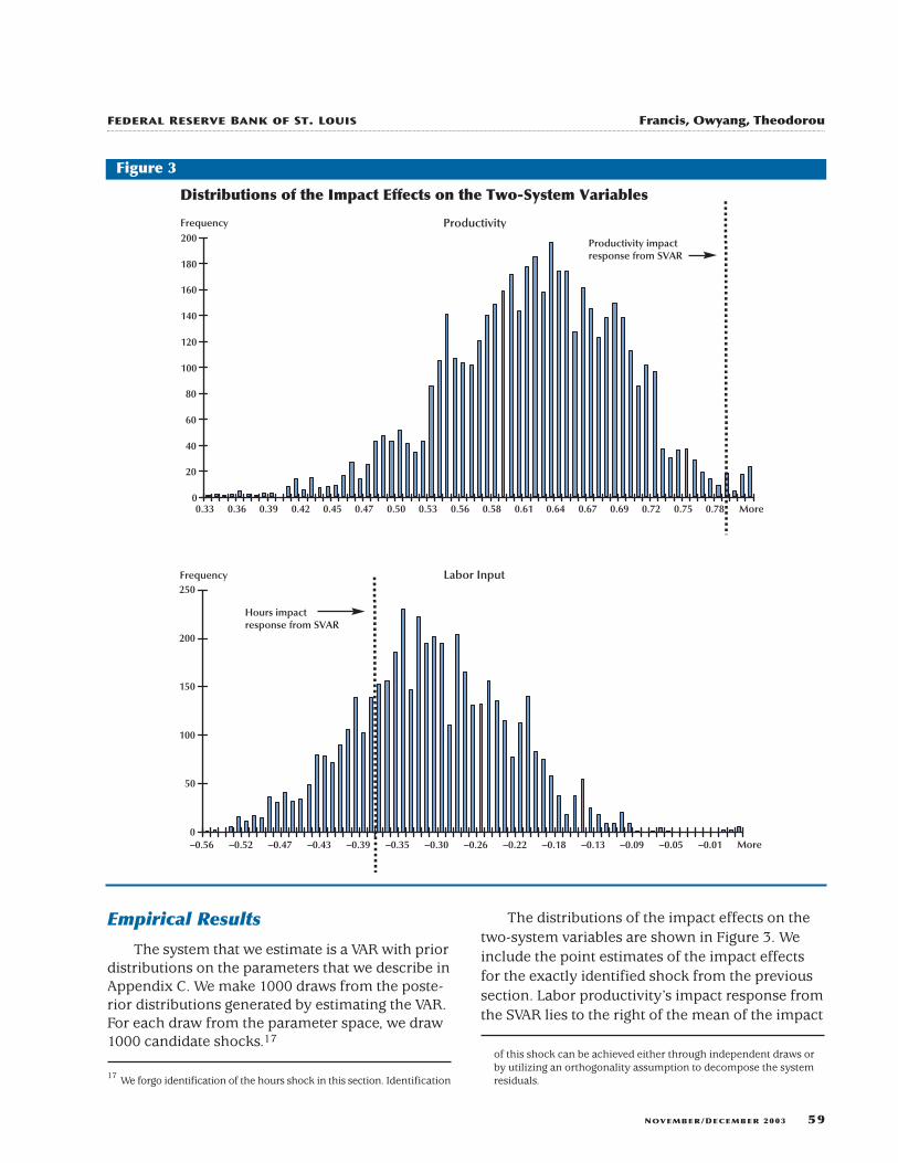
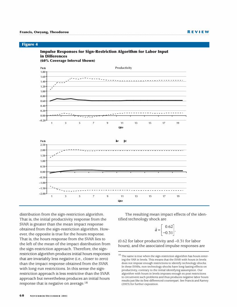
Impulse Responses for Sign-Restriction Algorithm for Labor Input in Differences(60% Coverage Interval Shown)

Quarter

Quarter

Figure 4

illustrated in Figure 4.19 For the long-horizon sign-restriction algorithm, we compute the responsesout to 40 quarters. Consistent with the findingsabove, this estimation presupposes that labor hourspossesses a unit root and is entered in differences.The productivity response to a technology shock ispositive on impact and converges to a steady-statevalue of 0.6 percent approximately eight periodsafter the initial shock. The algorithm imposes a risein labor productivity in the tenth year.20 However,

we note that the response to a technology shockfor the majority of prior periods turns out to alsobe positive.

Next, note that the average labor hours responseis negative on impact. In fact, in approximately 95percent of the accepted draws, the candidate tech-nology shock produces a negative response of hourson impact. However, on average, the decrease inhours is not permanent. Based on our findings usingthis impulse response–restricted algorithm, wecannot reject the hypothesis that a technology shockcauses labor hours to fall on impact. This conclusionstems from our ability to draw a variety of candidate

NOVEMBER/DECEMBER 2003 61

and impose that the productivity response from the 37th to the 40thperiods be positive.

FEDERAL RESERVE BANK OF ST. LOUIS Francis, Owyang, Theodorou

Productivity

0.40

0.60

0.80

1.00

1.20

1.40

1.60

1 3 5 7 9 11 13 15 17 19Quarter

Labor Input

–0.80

–0.60

–0.40

–0.20

0.00

0.20

0.40

0.60

1 3 5 7 9 11 13 15 17 19Quarter

Percent

Percent

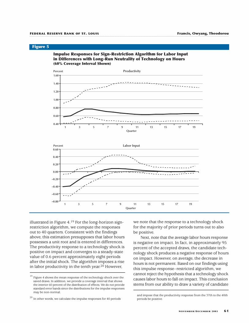
Impulse Responses for Sign-Restriction Algorithm for Labor Inputin Differences with Long-Run Neutrality of Technology on Hours(60% Coverage Interval Shown)

Figure 5

19 Figure 4 shows the mean response of the technology shock over thesaved draws. In addition, we provide a coverage interval that showsthe interior 60 percent of the distribution of effects. We do not providestandard error bands since the distributions for the impulse responsesmay be non-normal.

20 In other words, we calculate the impulse responses for 40 periods

shocks, which produce both long-run productivityresponses and negative hours responses.21

Finally, note that the coverage intervals inFigure 4 are relatively large compared with the errorbands associated with the SVAR in the precedingsection. Recall that the technology shock producedby the impulse response–restricted algorithm is notexactly identified—that is, the algorithm identifiesonly a distribution for the candidate shocks. Exactidentification requires further restrictions, and eachadditional (binding) restriction contributes to anarrowing in the coverage intervals. As an exampleof this, consider Figure 5. Here, we have identifiedthe technology shock with the additional restrictionthat imposes long-run neutrality of technology onhours, i.e., the impulse response of hours to a tech-nology shock is negligible at long horizons. In par-ticular, notice that the coverage interval for the hoursresponse is much narrower and that, in this case,a positive hours response on impact is even lesslikely to occur.

CONCLUSION

Economists have long assumed that one of theprimary components of the business cycle is shocksto technology that produce long-run changes inlabor productivity. In this article, we surveyed somerecent papers that attempted to identify such shocks.We especially focused on papers using the SVARapproach, with its accompanying long-run restric-tions, to identify technology shocks.

Recent results using the SVAR approach toidentify technology shocks have shown that theyinduce a negative impact response of labor hours.Further, using a long-horizon impulse response–restricted system, we generated “technology” byassuming that it is the only shock with a long-horizonimpact (say, out to ten years) on labor productivity.Technology shocks generated with this methodologyinvariably produce the (non-standard) negative laborhours impact result. That is, the probability of havinga fall in hours is found to be greater than the proba-bility of having a rise in hours for technology gen-erated in this manner, regardless of whether theVAR is estimated with labor hours in levels or infirst differences.

Future research could apply the impulseresponse–restricted technique in larger macro-economic models instead of the bivariate model

employed here. From this we could examine whichtechnology shock, from labor hours in levels or infirst differences, produces the more plausibleimpulses for variables such as consumption, invest-ment, and real wages. Future research should alsoexamine which measure of technology stands upto the scrutiny of the Hall-Evans tests as per Francisand Ramey (2002).

REFERENCES

Basu, Susantu; Fernald, John and Kimball, Miles. “AreTechnology Improvements Contractionary?” InternationalFinance Discussion Papers 1998-625, Board of Governorsof the Federal Reserve System, September 1998.

Blanchard, Olivier Jean and Quah, Danny. “The DynamicEffects of Aggregate Demand and Supply Disturbances.”American Economic Review, September 1989, 79(4), pp.655-73.

Canova, Fabio and De Nicolo, Gianni. “Monetary DisturbancesMatter for Business Fluctuations in the G-7.” Journal ofMonetary Economics, September 2002, 49(6), pp. 1131-59.

Christiano, Lawrence J.; Eichenbaum, Martin and Vigfusson,Robert. “What Happens After a Technology Shock?” NBERWorking Paper No. 9819, National Bureau of EconomicResearch, July 2003.

Denison, Edward F. Accounting for Slower Growth: TheUnited States in the 1970s. Washington, DC: The BrookingsInstitution, 1979.

Evans, Charles L. “Productivity Shocks and Real BusinessCycles.” Journal of Monetary Economics, April 1992, 29(2),pp. 191-208.

Faust, Jon. “The Robustness of Identified VAR ConclusionsAbout Money.” Carnegie-Rochester Conference Series onPublic Policy, December 1998, 49(0), pp. 207-44.

Francis, Neville R. and Owyang, Michael T. “What Is aTechnology Shock? A Bayesian Perspective.” Unpublishedmanuscript, 2003.

___________ and Ramey, Valerie A. “Is the Technology-Driven Real Business Cycle Hypothesis Dead? Shocksand Aggregate Fluctuations Revisited.” NBER WorkingPaper No. 8726, National Bureau of Economic Research,January 2002.

___________ and ___________. “The Source of Historical

62 NOVEMBER/DECEMBER 2003

Francis, Owyang, Theodorou R E V I E W

21 We performed a similar analysis using labor hours in levels. We foundthat the hours response to a positive technology shock is still, onaverage, negative on impact.

Economic Fluctuations: An Analysis Using Long-RunRestrictions.” Unpublished manuscript, May 2003.

Gali, Jordi. “Technology, Employment, and the BusinessCycle: Do Technology Shocks Explain AggregateFluctuations?” American Economic Review, March 1999,89(1), pp. 249-71.

Hall, Robert E. “The Relation Between Price and MarginalCost in U.S. Industry.” Journal of Political Economy,October 1988, 96(5), pp. 921-47.

___________. “Invariance Properties of Solow’s Residual,”in Peter Diamond, ed., Growth, Productivity,Unemployment. Cambridge, MA: MIT Press, 1990.

Kiley, Michael T. “Labor Productivity in U.S. Manufacturing:Does Sectoral Comovement Reflect Technology Shocks?”Unpublished manuscript, 1998.

King, Robert G.; Plosser, Charles I.; Stock, James H. andWatson, Mark W. “Stochastic Trends and EconomicFluctuations.” American Economic Review, September1991, 81(4), pp. 819-40.

___________ and Rebelo, Sergio T. “Resuscitating RealBusiness Cycles,” in Handbook of Macroeconomics.Volume 1B. New York: Elsevier Science, North-Holland,1999, pp. 927-1007.

Mountford, Andrew and Uhlig, Harald. “What Are theEffects of Fiscal Policy Shocks?” Discussion Paper 3338,Centre for Economic Policy Research, April 2002.

Owyang, Michael T. “Modeling Volcker as a Non-Absorbing

State: Agnostic Identification of a Markov-Switching VAR.”Working Paper 2002-018A, Federal Reserve Bank of St.Louis, 2002.

Rasche, Robert H. “Identification of Dynamic EconomicModels from Reduced Form VECM Structures: AnApplication of Covariance Restrictions.” Working Paper2000-011B, Federal Reserve Bank of St. Louis, 2001.

Shapiro, Matthew D. and Watson, Mark W. “Sources ofBusiness Cycle Fluctuations,” in Stanley Fischer, ed.,NBER Macroeconomics Annual 1988, Volume 3.Cambridge, MA: MIT Press, 1988, pp. 111-48.

Shea, John. “What Do Technology Shocks Do?” in BenBernanke and Julio Rotemberg, eds., NBER MacroeconomicsAnnual 1998. Volume 13. Cambridge, MA: MIT Press,1999, pp. 275-310.

Solow, Robert M. “Technical Change and the AggregateProduction Function.” Review of Economics and Statistics,August 1957, 39, pp. 312-20.

Uhlig, Harald. “What Are the Effects of Monetary Policy onOutput? Results from an Agnostic IdentificationProcedure.” Research Discussion Paper 28, TilburgUniversity, Center for Economic Research, 1999.

___________. “Did the FED Surprise the Market in 2001? ACase Study for VARs with Sign Restrictions.” DiscussionPaper 88, Tilburg University, Center for EconomicResearch, 2001.

___________. “Do Productivity Shocks Lead to a Decline inLabor?” Unpublished manuscript, 2002.

NOVEMBER/DECEMBER 2003 63

FEDERAL RESERVE BANK OF ST. LOUIS Francis, Owyang, Theodorou

Recall from (1) the MA representation of theVAR, reproduced here for convenience:

Yt=C(L)εt,

where we have implicitly assumed that C(L) isinvertible, C(L)–1=Φ(L), Φ(L) is the matrix polyno-mial in the lag operator, and the roots of |Φ(z)| areoutside the unit circle. From the assumption thatonly technology can have long-run effects on pro-ductivity, C(1) is lower triangular, which impliesthat Φ(1) is also lower triangular.22

The first equation of Φ(L)Yt=εt then becomes

(A.1.1) .

Since Φ(1) is lower triangular, the long-run multi-plier on ∆nt is identically zero, so the coefficientsof its lags sum to zero. (Note, we do not imposeany short-run dynamics so the contemporaneousvalue of ∆nt appears in the productivity (∆xt)equation.)

Imposing this constraint yields

.

The preceding equation is only a matter of algebra.The equivalence of the two methods is shown inthe example below for a particular lag length.

Set p=4.23 Then, rewrite (A.1.1) as

∆ ∆ ∆x x nt xx j t j xn j t j tx

j

p

j

p= + +∑∑ − −

=

−

=α β ε, ,

2

0

1

1

∆ ∆ ∆x x nt xx j t j xn j t j tx

j

p

j

p= + +∑∑ − −

==α α ε, ,

01

(A.1.2)

In this case, the long-run restriction C12(1)=0 of

lower triangularity implies

(A.1.3)

Thus, we have

Restriction (A.1.3) implies that the coefficient on∆nt –4 is identically zero. Thus, we have

(A.1.4)

We rewrite this as

(A.1.4′ ) ,

where the βs are functions of the αs. Note thatequation (A.1.4′ ) here is identical to (3).

The hours equation (4) is straightforward. Notethat we do not require the contemporaneous valueof ∆xt in the hours equation since ε t

x enters intoequation (4) directly.

∆ ∆ ∆x x nt xx j t j xn j t j tx

jj= + +∑∑ − −

==α β ε, ,

2

0

3

1

4

∆ ∆ ∆ ∆

∆

+ ∆ +

2 2

2

2

x x n n

n

n

t xx j t j xn t xn xn tj

xn xn xn t

xn xn xn xn t tx

= + + +( )∑

+ + +( )+ + +( )

− −=

−

−

α α α α

α α α

α α α α ε

, , , ,

, , ,

, , , , .

0 0 1 11

4

0 1 2 2

0 1 2 3 3

= +∑

+ ++ + ++ +

−=

−

− −

− −

α α

α αα α α

α

xx j t jj

xn t t

xn xn t t

xn xn xn t t

xn

x n n

n n

n n

, ,

, ,

, , ,

,

]

[ ] ( )

[ ] ( )

[

∆ [∆ − ∆

∆ − ∆∆ − ∆

1

4

0 1

0 1 1 2

0 1 2 2 3

0 ∆ − ∆∆

α α αα α α α α

xn xn xn t t

xn xn xn xn xn t

n n

n, , ,

, , , , ,

] ( )

[ ]1 2 3 3 4

0 1 2 3 4 4

+ ++ + + + +

− −

− .

∆ ∆ ∆ ∆

∆ ∆ ∆

x x n n

n n n

t xx j t j xn t xn tj

xn t xn t xn t

= + +∑

+ + +

− −=

− − −

α α α

α α α

, , ,

, , ,

0 1 11

4

2 2 3 3 4 4

α α α α αxn xn xn xn xn, , , , ,0 1 2 3 4 0+ + + + = .

∆ ∆ ∆ ∆∆ ∆ ∆

∆ ∆ ∆

x x x x

x n n

n n n

t xx t xx t xx t

xx t xn t xn t

xn t xn t xn t tx

= + ++ + +

+ + + +

− − −

− −

− − −

α α αα α α

α α α ε

, , ,

, , ,

, , ,

1 1 2 2 3 3

4 4 0 1 1

2 2 3 3 4 4 .

64 NOVEMBER/DECEMBER 2003

Francis, Owyang, Theodorou R E V I E W

Appendix A

22 We are essentially imposing that the system is a Wold causal chainstructure in the steady state.

23 We arbitrarily choose four lags, but the results will hold true forany general lag length.

Consider the reduced-form VAR

A(L)Yt=et,

where A(L) is an (n×n) matrix of lag polynomialsand et ∼ N(0,Σ). We can rewrite this VAR in its MA(`)representation:

Yt=B(L)et,

where B(L)=A(L)–1. The model residuals et haveno structural interpretation; the objective of thisexercise is to identify the structural shocks εtdefined in the third section, on implementing long-run restrictions. This can be accomplished byimposing restrictions on either the contemporaryimpact matrix or by imposing effect restrictionson the long-run multipliers Cij(1) defined in (2).Once the structural shocks εt are identified, thes-period-ahead response to shock εt

i can be com-puted by

(A.2.1) ,∂

∂=+E Y

YCt s

ti s t

i( ) ε

where Cs is the lag-s matrix derived from the MArepresentation, Cs=Bs*R and εt=R–1et. R is a(rotation) matrix that maps the reduced form intothe structural form and, thus, depends on thenature of the restrictions imposed.

Since B(L) is generated from the reduced-formestimation, one can easily see that sufficient restric-tions on the left-hand side of (A.2.1) can be usedto uniquely identify C(L) and εt

i. The alternativeidentification that we impose in the fourth sectionof the paper takes a decidedly different tack. Insteadof imposing restrictions on either the contempo-rary impact matrix or the long-run multipliers,we restrict the impulse responses (A.2.1) directly.Since our algorithm imposes only sign restrictions,which may not be binding, we do not exactlyidentify the structural shock. Instead, we mustdraw candidate shocks and test whether the signrestrictions are violated. This allows us to identifya distribution of structural shocks, which we use totest the robustness of the conclusions drawn fromthe estimation in the third section of the paper.

NOVEMBER/DECEMBER 2003 65

FEDERAL RESERVE BANK OF ST. LOUIS Francis, Owyang, Theodorou

Appendix B

Appendix C

We begin with the reduced-form, four-lag VAR:

(A.3.1) ,

where the Di are the lag-i coefficient matrices,I– D(L)=A(L), and the ei are the i.i.d. reduced-form residuals with covariance matrix Σ. It isconvenient to stack the system (A.3.1) in the follow-ing manner:

(A.3.2) Y=XD+e ,

where D=[D1,D2,…Dk ]′, Y=[y1,y2,…yT]′,Xt=[ y′t –1, y′t –2,…y′t –k]′, X=[X1, X2,…XT]′, ande=[e1,e2,…eT]′. Here, T is the sample length and kis the lag order (k=4 in our case).

The system (A.3.2) can be estimated as a VARwith a normal-inverted Wishart prior conjugatedistribution with parameters v0, N0, δ0, and S0.Then, the VAR parameters can be drawn from thejoint posterior distribution, also a normal-invertedWishart distribution centered on δ and S with vdegrees of freedom and precision matrix N. The

Y D Y et ii

t i t= ∑ +=

−1

4

parameters for the posterior distribution aregiven by

,

,

,

,

where DX=(X′X)–1X′Y and Σ̂=(Y–XDX)′ (Y–XDX).24

We can characterize the impulse vector θ̂ by

θ̂=Qq,

where QQ′=Σ is the Cholesky decomposition ofthe state-dependent covariance matrix and q is avector drawn from the unit circle. The Choleskyfactorization does not impose a causal ordering

Svv

STv v

D N N D= + + − ′ ′ −−00 0 0

10

1Σ̂ ( ) ( )) )

δ δX X

δ δ= + ′−N N D10 0( )X X

)

N N= + ′0 X X

v T v= + 0

24 In estimating the Bayesian VAR (A.3.2), we utilize uninformative priors.That is, we assume v0=0 and N0=0

∼n, with S0 and δ0 arbitrary. This

makes (A.3.2) a simple reduced-form VAR.

in this case but provides a means of orthogonalizingthe shocks.25 We then apply (A.3.3) and (A.3.4) togenerate impulse responses and test them againstthe restriction matrix R. Any θ̂ that satisfies therestrictions on yt+j is retained. Multiple iterationsover a single set of sampled model parametersyield a distribution for the shocks, Θ(D,Σ,R).26

Suppose the impulse response to any vectorinnovation θ̂ can be defined as

(A.3.3) ,∆ Γyt jj

+ = θ

where θ–=[θ̂ ′,01×2(k–1)]′ and the (2k × 2k) impulse-generating matrix Γ is defined by

(A.3.4) .

Here, D is the stacked coefficient matrix, I2(k–1)is the 2(k –1) × 2(k –1) identity matrix and 0∼2(k–1)× 2is a 2(k –1) × 2 matrix of zeros.

The algorithm for identifying the technologyshock is as follows: The impulse response to anyshock θ̂ can be calculated using (A.3.3) and (A.3.4).The shock θ̂ is associated with a restriction matrixR that is invariant to the state of the economy. R isan (n × l ) matrix that represents the priors that weimpose on the response of model variables to theincidence of a shock θ̂ out to a horizon l. Ouridentification centers on the selection of the shockθ̂ that produces an impulse response satisfyingthe restriction matrix R.

Γ =′

− − ×

D

I k k2 1 2 1 20( ) ( )˜

66 NOVEMBER/DECEMBER 2003

25 See Mountford and Uhlig (2002) for a discussion of the use of theCholesky factorization.

26 Our characterization of the impulse vector space is slightly differentfrom Uhlig (1999). He implicitly assumes that the sign restrictionson the impulse response functions hold out to horizon l, and hecharacterizes the space as Θ(D,Σ,l ). Since we will impose long-runrestrictions, it is beneficial to denote the impulse vector space asdependent on a restriction matrix R.

Francis, Owyang, Theodorou R E V I E W