S F

B XXX

E

C O

N O

M I

C

R I

S K

B

E R

L I

N

SFB 649 Discussion Paper 2014-009

Structural Vector Autoregressions:

Checking Identifying

Long-run Restrictions via Heteroskedasticity

Helmut Lütkepohl*/** Anton Velinov**

* Freie Universität Berlin, Germany

** DIW, Germany

This research was supported by the Deutsche

Forschungsgemeinschaft through the SFB 649 "Economic Risk".

http://sfb649.wiwi.hu-berlin.de

ISSN 1860-5664

SFB 649, Humboldt-Universität zu Berlin Spandauer Straße 1, D-10178 Berlin

SFB

6

4 9

E

C O

N O

M I

C

R I

S K

B

E R

L I

N

January 18, 2014

Structural Vector Autoregressions:

Checking Identifying Long-run Restrictions

via Heteroskedasticity1

Helmut LutkepohlDepartment of Economics, Freie Universitat Berlin and DIW Berlin

Mohrenstr. 58, D-10117 Berlin, Germanyemail: hluetkepohl@diw.de

Anton VelinovDIW Berlin

Mohrenstr. 58, D-10117 Berlin, Germanyemail: avelinov@diw.de

Abstract. Long-run restrictions have been used extensively for identify-ing structural shocks in vector autoregressive (VAR) analysis. Such restric-tions are typically just-identifying but can be checked by utilizing changes involatility. This paper reviews and contrasts the volatility models that havebeen used for this purpose. Three main approaches have been used, exoge-nously generated changes in the unconditional residual covariance matrix,changing volatility modelled by a Markov switching mechanism and multi-variate generalized autoregressive conditional heteroskedasticity (GARCH)models. Using changes in volatility for checking long-run identifying restric-tions in structural VAR analysis is illustrated by reconsidering models foridentifying fundamental components of stock prices.

Key Words: Vector autoregression, heteroskedasticity, vector GARCH, con-ditional heteroskedasticity, Markov switching model

JEL classification: C32

1This paper was written while the first author was a Bundesbank Professor. Thisresearch was supported by the Deutsche Forschungsgemeinschaft through the SFB 649“Economic Risk”.

1 Introduction

An important problem in vector autoregressive (VAR) analysis is that the

reduced form residuals are typically not the shocks that are of interest from

an economic point of view. Determining shocks of economic interest is a

main subject of structural VAR (SVAR) analysis. Proposals have been made

how to identify shocks by placing restrictions on the impact effects, the

long-run responses of the variables, or the signs of the impulse responses.

More recently it has been discussed how to utilize changes in the volatility

of the residuals or the variables for getting identifying information for the

shocks. Important work on that topic is due to Rigobon (2003), Rigobon

and Sack (2003), Normandin and Phaneuf (2004), Lanne and Lutkepohl

(2008a), Bouakez and Normandin (2010) and Lanne, Lutkepohl and Ma-

ciejowska (2010). A survey of that literature appears in Lutkepohl (2013a).

In this study we first present a unifying framework for identifying struc-

tural shocks by imposing long-run restrictions possibly in combination with

restrictions on the short-run effects. The latter are typically zero restrictions

on the impact effects while long-run restrictions usually specify that specific

shocks do not have a long-lasting or permanent effect on some of the vari-

ables whereas other shocks may have persistent effects. For example, in an

important study in this context, Blanchard and Quah (1989) assume that

demand shocks do not have permanent effects on output while the long-run

impact of supply shocks is not restricted. Long-run effects of shocks are

possible if some of the variables are integrated and, hence, have some per-

sistence. In the Blanchard-Quah approach it is typically assumed that some

variables appear in growth rates and the effects of the shocks on the levels

or log-levels may be permanent. Thus, the variables enter in transformed

stationary form in the VAR model. Such an approach is justified if there is

no cointegration between the levels variables. For the case of cointegrated

variables it is preferable to set up a vector error correction (VEC) model.

King, Plosser, Stock and Watson (1991) propose an approach for imposing

long-run restrictions for shocks in such cointegrated VAR models. It also

1

allows for restrictions on the impact effects of shocks. As shown by Fisher

and Huh (2014), other approaches of imposing long-run restrictions on SVAR

models can be cast in this modelling framework as well. We first present the

King et al. (1991) approach as a unifying framework for imposing long-run

and short-run restrictions in SVAR models and then discuss the relation to

the literature on identification via heteroskedasticity.

The long-run and short-run restrictions used for identifying structural

shocks in VAR models are typically just-identifying. Hence, they can not

be tested in a conventional framework. We show how changes in volatility

can be used to obtain additional identifying information that can be used

to test restrictions that are just-identifying in a conventional framework. To

this end we give a brief survey of the main approaches that have been used

for identifying SVARs through heteroskedasticity. Our review draws partly

on Lutkepohl (2013a) but is more condensed and less technical. In contrast

to Lutkepohl (2013a) we will pay special attention to VAR models with

integrated and cointegrated variables.

Illustrative examples are presented from the literature that investigates

the impact of fundamental shocks on stock prices. Since financial market

series are often characterized by changes in volatility or conditional het-

eroskedasticity they have features that are an important precondition for

applying the techniques developed in the related literature. Moreover, the

identifying restrictions used in this context are sometimes on soft grounds so

that bringing in alternative sources for identification is desirable.

This study is organized as follows. The general model setup is presented

in Section 2. Specific models for changes in volatility that are useful for

providing additional identifying information for shocks in SVAR models are

reviewed in Section 3. Illustrations based on studies from the literature on the

importance of fundamental shocks for stock price movements are discussed

in Section 4 and conclusions are presented in Section 5.

2

2 SVARs with Integrated and Cointegrated

Variables

We start from a K-dimensional reduced form VAR(p) model,

yt = ν + A1yt−1 + · · ·+ Apyt−p + ut, (1)

where ν is a (K×1) constant term, Aj (j = 1, . . . , p) are (K×K) VAR coeffi-

cient matrices and ut is a zero-mean white noise error term with nonsingular

covariance matrix Σu, that is, ut ∼ (0,Σu). Considering more general deter-

ministic terms is easily possible. We avoid them in our basic model because

they are of no importance for the structural analysis we are interested in.

The components of yt may be integrated and cointegrated variables. For

simplicity we assume that all variables are stationary (I(0)) or integrated of

order one (I(1)). For our empirical example in Section 4 this assumption

is general enough and it also covers the majority of examples in the related

literature. Hence, it makes sense to avoid complications resulting from more

general assumptions regarding the integration properties of the variables. If

there are integrated variables, using the vector error correction (VEC) form

of model (1) is often helpful. Assuming that there are r linearly independent

cointegration relations, it can be written as

∆yt = ν + αβ′yt−1 + Γ1∆yt−1 + · · ·+ Γp−1∆yt−p+1 + ut, (2)

where ∆ is the differencing operator such that ∆yt = yt−yt−1, η is a (K×1)

constant term, α is a (K × r) loading matrix, β is a (K × r) cointegration

matrix and Γ1, . . . ,Γp−1 are (K×K) coefficient matrices (see, e.g., Lutkepohl

(2005) for the relation between the parameters in (1) and (2)).

SVAR analysis with homoskedastic reduced form residuals ut assumes

that the structural shocks, εt, are obtained from the reduced form residuals

by a linear transformation εt = B−1ut. In other words, Bεt = ut, where B

is such that the structural shocks are instantaneously uncorrelated, that is,

εt ∼ (0,Σε), and Σε is a diagonal matrix. In fact, the structural variances

3

are often normalized to one so that Σε = IK and, hence, B is such that

Σu = BB′. The matrix B is not uniquely determined by this relation. In

fact, at least K(K − 1)/2 further relations or restrictions are needed for

uniquely identifying B.

Substituting Bεt for ut in (1) or (2) the matrix B is easily recognized as

the matrix of impact effects of the structural shocks. Thus, imposing restric-

tions on the impact effects constrains the elements of B directly. Exclusion

restrictions are quite common in this context. In other words, a certain shock

may be assumed to have no instantaneous effect on a particular variable. A

recursive structure which implies a triangular B matrix is not uncommon in

this framework. Exclusion restrictions are also often imposed on the instan-

taneous relations of the observed variables yt. Such restrictions amount to

restricting B−1. Of course, a triangular matrix B−1 implies also a triangular

matrix B.

Restrictions on the long-run effects of the shocks have also been used fre-

quently for identifying B. To see how this is done it may be useful to consider

the matrix of long-run effects of the reduced form errors from the Granger-

Johansen representation (see Johansen (1995)) of the yt corresponding to (2),

Ξ = β⊥

[α′⊥

(IK −

p∑i=1

Γi

)β⊥

]−1α′⊥, (3)

where β⊥ and α⊥ are (K × (K − r)) dimensional orthogonal complements of

the (K × r) dimensional matrices β and α, respectively (see, e.g., Lutkepohl

(2005, Chapter 9) for details). If the cointegration rank r is zero, the orthog-

onal complements matrices are simply replaced by (K×K) identity matrices

so that the long-run effects matrix becomes

Ξ =

(IK −

p−1∑i=1

Γi

)−1. (4)

In each case the corresponding long-run effects of the structural shocks are

given by ΞB. Since α and β have rank r if the cointegration rank is r, their

4

orthogonal complements have rank (K − r). Hence, Ξ also has rank (K − r)and the same holds for ΞB because B is of full rank K. As a consequence,

there can only be at most r shocks without any long-run effects because there

can be at most r columns of zeros in ΞB. Generally, for a given Ξ matrix,

restricting the product ΞB implies restrictions for B and, hence can help

identify the structural shocks. Identification of the structural shocks in this

framework is discussed by King et al. (1991) and an introductory account is

given in Lutkepohl (2005, Chapter 9). Therefore we do not provide a full

discussion here but just mention two specific issues for later reference that

have to be taken into account: (1) Shocks without any long-run effect at

all (with corresponding zero column in ΞB) need to be identified by other

restrictions such as zero restrictions on the impact effects. Of course, if there

is just one such shock, there is no need for further restrictions to identify

that shock. (2) Since the rank of ΞB is (K− r), it is in general not sufficient

to identify all shocks by K(K − 1)/2 restrictions on the matrix of long-run

effects.

Because the case of a cointegration rank of zero is of specific interest,

it may be worth discussing that situation in a little more detail here. As

mentioned before, for r = 0 the matrix of long-run effects ΞB is of full

rank K and, hence, there cannot be shocks with no long-run effects at all,

that is, there cannot be zero columns in ΞB. Thus, all K structural shocks

have some long-run effects and it turns out that they can be identified via

K(K−1)/2 suitable restrictions on ΞB. For example, restricting this matrix

to be triangular is sufficient. Of course, if the cointegrating rank is zero, the

VEC model (2) reduces to a VAR model in first differences,

∆yt = ν + Γ1∆yt−1 + · · ·+ Γp−1∆yt−p+1 + ut,

for which the accumulated long-run effects on the ∆yt are known to be (IK−∑p−1i=1 Γi)

−1B. The accumulated effects on the first differences are just the

long-run effects on the levels yt. Considering the accumulated effects of

a stationary system is of particular interest in this context because in a

number of applied studies the restrictions and shocks are set up such that

5

the accumulated long-run effects matrix is triangular. This case was first

considered by Blanchard and Quah (1989) and in that case estimation of the

structural parameters, i.e., the B matrix, is particularly easy (e.g., Lutkepohl

(2005, Chapter 9)). We see another example in Section 4.

There is a large body of literature on long-run restrictions for identifying

structural shocks in VARs. For example, there are proposals by Gonzalo

and Ng (2001), Fisher, Huh and Summers (2000), and Pagan and Pesaran

(2008). Fisher and Huh (2014) review that literature and discuss the relations

between the various approaches. In the present context it is not important

which approach is used for imposing long-run restrictions. They can all

be combined with the identification procedures derived from time varying

volatility discussed in the next section.

3 SVAR Models with Changes in Volatility

3.1 General Setup

So far we have discussed restrictions on the short- and long-run effects of

shocks, that is, restrictions onB directly or via the restrictions on ΞB to make

B unique for a given reduced form error covariance matrix Σu. Another way

of getting a unique B matrix is available if there are two different covariance

matrices, say Σ1 and Σ2, for example, if E(utu′t) = Σ1 in the first part of the

sample, say for t = 1, . . . , T1, and E(utu′t) = Σ2 in the second part of the

sample (t > T1). Then it is known from matrix algebra that there exists a

matrix B and a diagonal matrix Λ = diag(λ1, . . . , λK) such that

Σ1 = BB′ and Σ2 = BΛB′. (5)

Using this B matrix to obtain structural shocks from the reduced form errors

as εt = B−1ut, gives

E(εtε′t) =

{IK , t = 1, . . . , T1,

Λ, t > T1.

6

These shocks satisfy the basic requirement of being instantaneously uncor-

related because Λ is diagonal. In fact, the matrix B is unique apart from

changes in the signs and permutations of the columns if the diagonal ele-

ments of Λ are all distinct (Lanne et al. (2010)). In other words, if the

latter condition holds, unique shocks are obtained by just imposing the basic

requirement that they have to be instantaneously uncorrelated.

Note, however, that using the same transformation matrix B for the whole

sample period, that is, for both volatility states, implies that the impact

effects of the shocks are time-invariant and only the variances differ across

states. All other requirements for uniqueness of the joint decomposition

of the two covariance matrices do not affect the shocks substantively. The

possibility for changing the sign of a column just means that we may consider

negative instead of positive shocks and vice versa. Moreover, permuting

columns of the B matrix just changes the ordering of the shocks and that

can be chosen freely, as usual in SVAR analysis. Thus, fixing some ordering

of the shocks and their sign is not restrictive.

Of course, the unique shocks obtained in this way may not be shocks

of economic interest. That cannot be expected because no economics has

been used in constructing them. However, if our minimal assumptions lead

to unique shocks, then any further restrictions become over-identifying and,

hence, testable. For example, if economic considerations suggest restrictions

on the long-run effects of the shocks, these restrictions become testable in

our framework even if they are just-identifying in a conventional setting and

this is what makes it attractive to use changes in volatility in this context.

Of course, there may be more than two volatility regimes. If there are

M > 2 regimes with corresponding covariance matrices Σ1, . . . ,ΣM , the de-

composition

Σ1 = BB′, Σm = BΛmB′, m = 2, . . . ,M, (6)

with diagonal matrices Λm = diag(λm1, . . . , λmK) (m = 2, . . . ,M) may not

exist. Hence, the decomposition (6) imposes testable restrictions on the co-

variance matrices. Therefore it can be checked with a statistical test whether

7

the data are compatible with the decomposition and, hence, we can use B

to transform the reduced form residuals into structural errors with time-

invariant impact effects. Uniqueness of B (apart from ordering and sign) in

this case follows if for any two subscripts k, l ∈ {1, . . . , K}, k 6= l, there is

a j ∈ {2, . . . ,M} such that λjk 6= λjl (Lanne et al. (2010, Proposition 1)).

This identification condition has the advantage of being testable because, if

there are M distinct volatility regimes, then the diagonal elements of the

Λm matrices are identified and, hence, can be estimated consistently with a

proper asymptotic distribution under common assumptions.

So far we have just considered finitely many volatility states. If condi-

tional heteroskedasticity is generated by a GARCH process, then there is a

continuum of conditional covariance matrices Σt|t−1. We discuss this case in

more detail below and therefore just mention here that it can also be used

for identifying shocks in SVAR models in much the same way as for finitely

many covariance matrices. It should be clear by now that having two dif-

ferent covariance matrices is crucial for getting unique shocks. Having more

covariance matrices is an advantage but not required for identification via

changes in volatility.

3.2 Specific Models for Changes in Residual Volatility

Three main assumptions regarding the changes in volatility have been used

in the SVAR literature: (1) exogenous changes in the unconditional residual

covariance matrices in given time periods, (2) changes in the residual volatil-

ity generated by a Markov regime switching mechanism, and (3) volatility

changes generated by a vector generalized autoregressive conditional het-

eroskedasticity (MGARCH) process. These three approaches will be pre-

sented formally in the following.

Assuming M exogenously determined volatility regimes, the reduced form

residual covariance matrix in time period t can be represented as

E(utu′t) = Σt = Σm if t ∈ Tm, (7)

8

where Tm = {Tm−1 + 1, . . . , Tm} (m = 1, . . . ,M) are M given volatility

regimes. Here it is assumed that T0 = 0 and TM = T . The volatility

change points Tm, for m > 0, are usually assumed known to the econome-

trician or they are determined with some preliminary statistical procedure.

Rigobon (2003) considers this type of model of changes in the unconditional

residual variance in his original article on identifying structural shocks in

SVARs through heteroskedasticity. He also considers the possibility of mis-

specifying the change points. This type of model was also used in applica-

tions by Rigobon and Sack (2004), Lanne and Lutkepohl (2008a, 2008b) and

Ehrmann, Fratzscher and Rigobon (2011).

If the reduced form error term is normally distributed, ut ∼ N (0,Σt), the

model can be estimated by maximum likelihood (ML) (see, e.g., Lutkepohl

(2005, Chapter 17) for details). If the errors are not normal, maximizing the

Gaussian log-likelihood can be justified as a quasi ML estimation procedure

or a GLS procedure may be used (see Lutkepohl (2013a)). In any case, if the

VEC form of the VAR model is used, estimating the cointegration relations

first from a reduced form VEC model and then keeping them fixed in the

structural estimation may be useful. The estimators have standard asymp-

totic properties under common assumptions that can be used for inference

in these models.

Another approach assumes that the volatility changes are generated en-

dogenously within the model by a Markov regime switching (MS) mechanism.

More precisely, the reduced form error term ut is assumed to depend on a dis-

crete, first order Markov process st (t = 0,±1,±2, . . . ) with M states, that

is, st ∈ {1, . . . ,M} and transition probabilities pij = Pr(st = j|st−1 = i),

i, j = 1, . . . ,M . This model was first considered in the present context by

Lanne et al. (2010) who also propose a ML estimation procedure based on

conditionally normally distributed ut,

ut|st ∼ N (0,Σst). (8)

If the transition probabilities p1j = · · · = pKj = Pr(st = j), the state

associated with period t is independent of the states of previous periods and

9

we get a model with mixed normal residuals. In the present context such

models are considered by Lanne and Lutkepohl (2010).

The MS model is in some sense rather restrictive because it does not al-

low the VAR coefficients to vary over time. Thus, it is more restrictive than

the related models considered by Rubio-Ramirez, Waggoner and Zha (2005),

Sims and Zha (2006) and Sims, Waggoner and Zha (2008), for example. The

latter authors do not use the changes in volatility for identification of shocks,

however, and, as we have discussed in Section 3.1, to use that device requires

at least some time-invariance of the VAR coefficients. The M different co-

variance matrices corresponding to the different states of the Markov process

are used for the identification of the shocks just as explained in Section 3.1.

Notice that the model assumes conditional heteroskedasticity of the residu-

als. Moreover, it does not require the residuals to be in a particular state in

each sample period but allows for the possibility that a particular period is

in-between states by assigning a weighted sum of the states to it. Thus, the

model can capture quite general forms of conditional heteroskedasticity as it

is sometimes assumed to be present in financial time series.

ML estimation of these models is rather difficult, especially if there are

many variables, lags and/or Markov process regimes. Herwartz and Lutkepohl

(2011) discuss the related problems and present an EM algorithm based on

Krolzig (1997). In practice the number of states for a suitable representation

of the data will be unknown. Psaradakis and Spagnolo (2003, 2006) con-

sider standard model selection criteria for selecting the number of Markov

states and find that they work reasonably well. In contrast, standard testing

procedures suffer from the problem that some parameters in the alternative

model will not be identified if the null hypothesis imposes a reduced number

of states. Hence, the usual tests have nonstandard properties (e.g., Hansen

(1992), Garcia (1998)).

The model has been used in a number of applications. Examples are

Lutkepohl and Netsunajev (2013), Herwartz and Lutkepohl (2011), Netsunajev

(2013) and Velinov (2013) (see Lutkepohl (2013a) for a summary of some of

10

that work). Moreover, Lanne and Lutkepohl (2010) apply their special case

model with mixed normal residuals.

As mentioned earlier, the MS model can capture quite general forms of

conditional heteroskedasticity. It may still be attractive in some situations

to consider standard MGARCH models as alternatives if conditional het-

eroskedasticity is diagnosed. Normandin and Phaneuf (2004) propose these

kinds of models for the SVAR context.

In their approach the reduced form errors ut are assumed to be generated

by an MGARCH process of the form

Σu,t|t−1 = E(utu′t|ut−1, . . . ) = BΣε,t|t−1B

′, (9)

where Σε,t|t−1 = diag(σ21,t|t−1, . . . , σ

2K,t|t−1) is a diagonal matrix with

σ2k,t|t−1 = γk0 +

q∑j=1

γkjε2t−j +

s∑j=1

gkjσ2k,t−j|t−j−1, k = 1, . . . , K. (10)

In this setup the structural shocks, εt, are assumed to be instantaneously

uncorrelated and have a diagonal MGARCH(q, s) structure. This type of

model is sometimes called a generalized orthogonal GARCH (GO-GARCH)

model and was proposed earlier by van der Weide (2002) and a closely related

version is due to Vrontos, Dellaportas and Politis (2003). The standard model

in the GARCH literature is actually an MGARCH(1,1) model and this is also

the model considered by Normandin and Phaneuf (2004).

General identification conditions for this type of model are given by Sen-

tana and Fiorentini (2001). They show that the structural shocks are identi-

fied (apart from sign changes and permutations) if the matrix Γ′Γ is invert-

ible, where Γ′ is a matrix with kth row (σ2k,1|0, . . . , σ

2k,T |T−1). Invertibility of

Γ′Γ means that the changes in volatility have to be sufficiently heterogeneous.

For instance, at most one component can have constant conditional variances.

If the identification conditions are satisfied and we choose εt = B−1ut with

the B matrix from (9), then the structural shocks are unique and the impulse

responses, including the impact effects, are time-invariant.

11

Normandin and Phaneuf (2004) propose a two-step procedure for param-

eter estimation that fits a reduced form VAR(p) process in the first step and

then estimates the GARCH and structural parameters by maximizing the

corresponding Gaussian log-likelihood. Obviously, the estimation problem is

a highly nonlinear optimization task that may pose a computational chal-

lenge for higher dimensional systems. Applications of the GARCH setup in

SVAR analysis are reported by Normandin and Phaneuf (2004) and Bouakez

and Normandin (2010).

In principle it is also possible to consider different types of MGARCH

models instead of the GO-GARCH. For example, Weber (2010) and Strohsal

and Weber (2012) consider a so-called SCCC MGARCH model. It does not

ensure uncorrelated structural errors and may hence be regarded as prob-

lematic from a standard structural modelling point of view. The advantage

of such alternative MGARCH models in the present context is not clear.

Therefore we do not discuss them in more detail here.

4 Models for Stock Price Fundamentals

This section illustrates how the identification through heteroskedasticity tech-

nique can be used in practice. In particular, popular multivariate time series

models dealing with stock price fundamentals are considered and their struc-

tural identification restrictions are tested so as to determine whether or not

they are supported by the data. The empirical analysis in this section draws

from the work of Velinov (2013) and extends it by examining impulse re-

sponses obtained from the structural models.

The topic of investigation is to what extent stock prices reflect their un-

derlying economic fundamentals. This issue has naturally received a lot of

attention in the empirical time series literature. In particular, many SVAR

and SVEC models investigating this topic are based on the dividend dis-

count model (DDM). The DDM claims that an asset’s price is the sum of its

expected future discounted payoffs (such as dividends). These pay-offs are

12

necessarily linked to real economic activity such as real GDP, industrial pro-

duction, company earnings and so on. An alternative view is that stock prices

are to a large extent driven by speculation and, hence, their dependence on

fundamentals is limited.

For illustrative purposes two of the models from Velinov (2013) are con-

sidered here. Both are trivariate models that have been used widely in the

literature. The first model, called Model I in the following, consists of real

GDP (Yt), real interest rates (rt) and real stock prices (st) ordered in that

fashion. The second model, Model II, consists of real earnings (Et) instead

of real GDP and the other variables are the same. In other words, for Model

I, yt = (Yt, rt, st)′, while for Model II, yt = (Et, rt, st)

′.

Both models are related to the DDM and differ only in the proxy they

use for real economic activity. They are both popular models. For instance,

Model I is used in Lee (1995), Rapach (2001)2, Binswanger (2004), Lanne and

Lutkepohl (2010) and Jean and Eldomiaty (2010), while Model II is used in

Binswanger (2004) and Jean and Eldomiaty (2010). They are also relatively

simple models, consisting of only three variables, and will hence serve as a

good illustration of the testing approach considered here.

The structural parameters in these models are identified by means of

restrictions on the long-run effects matrix, denoted as ΞB as in Section 2. In

particular, ΞB is always restricted to be lower triangular. In other words, the

last shock has no long-run effects on real economic activity and the interest

rate. Hence, many of the papers mentioned classify this as a non-fundamental

shock. In contrast, only the first shock is allowed to have permanent effects

on all the variables and in particular on the real GDP or real earnings variable

and, hence, it is classified as being fundamental.

As was discussed in Section 2, the relevant (long-run) restrictions depend

on the model used, i.e. whether it is in VEC or VAR form. Hence, before

formally stating the relevant identification schemes to be considered, a brief

2In the case of Rapach (2001), Model I is a subset of a larger model, however, the

identifying restrictions are the same.

13

(a) Y, s (b) r, E

Figure 1: Data used with recession dates indicated by shaded bars.

note on the data and some basic diagnostic tests is in order to justify the

model type.

4.1 Data and Model Specification

We use the same data as Velinov (2013). In other words, data on GDP,

interest rates, stock prices and CPI are from the Federal Reserve Economic

Database (FRED) whereas earnings data are from Robert Schiller’s web-

page.3 The data is quarterly and ranges from 1947:I - 2012:III for Model

I and until 2012:I for Model II, the slightly shorter range for Model II be-

ing due to missing observations on earnings for the last quarters of 2012. All

variables are in real terms and in logs (except for the real interest rate series).

The series are deflated by using the CPI inflation rate. Figure 1 plots the

data used along with recession periods according to NBER dating marked

by shaded bars.

Standard unit root tests indicate that all variables can be treated as I(1).

This is true even for the real interest rate series. Hence, Johansen (1995)

trace tests are used to check for cointegration. There is substantial evidence

of cointegration only for Model II, with a cointegration rank of one. Hence,

Model I is set up as VAR in first differences, as in (1), while Model II is a

3Found at http://www.econ.yale.edu/ shiller/data.htm.

14

VEC of the form (2) with r = 1.

The traditional structural restrictions for identifying the shocks can be

summarized as

ΞBSV AR =

? 0 0

? ? 0

? ? ?

and ΞBSV EC =

? 0 0

? ? 0

? ? 0

, (11)

for the SVAR, ΞBSV AR, and the SVEC, ΞBSV EC , case respectively. Here ?

denotes an unrestricted element. Note that the SVEC model has one more

zero for its long-run effects matrix. This is because the rank of ΞBSV EC

in the VEC model is K − r, which is 2 in our case, hence a full column of

zeros represents only 2 restrictions. Both identification schemes therefore give

three independent restrictions. These just-identify the structural parameters

in the traditional setup where volatility changes are ignored or at least not

used for identification. Thus, in the traditional setup the restrictions cannot

be checked with statistical tests. In the following it will be shown how changes

in volatility can be used for checking the restrictions.

4.2 Checking Traditional Identification Restrictions via

Changes in Volatility

In both models changes in volatility are modelled via Markov processes with

three states and the same VAR orders as in Velinov (2013), that is, Model

I is a MS(3)-VAR(2) and Model II is a MS(3)-VEC model with two lagged

differences of ∆yt in (2). Modelling changes in volatility by MS models makes

sense here because it is quite flexible by allowing a number of different states

and also mixtures of states. So it can capture conditional heteroskedastic-

ity of quite general form. The three-state models have some support from

standard model selection criteria and tests. The estimated state covariance

matrices are given in Table 1 together with tests for the decomposition (6).

The variance estimates (the diagonal elements of the covariance matrices)

tend to increase for each state, in particular for Model II. This means that

15

each state captures slightly more volatile periods. Hence, the states can be

classified as capturing periods of increasing volatility. The periods associated

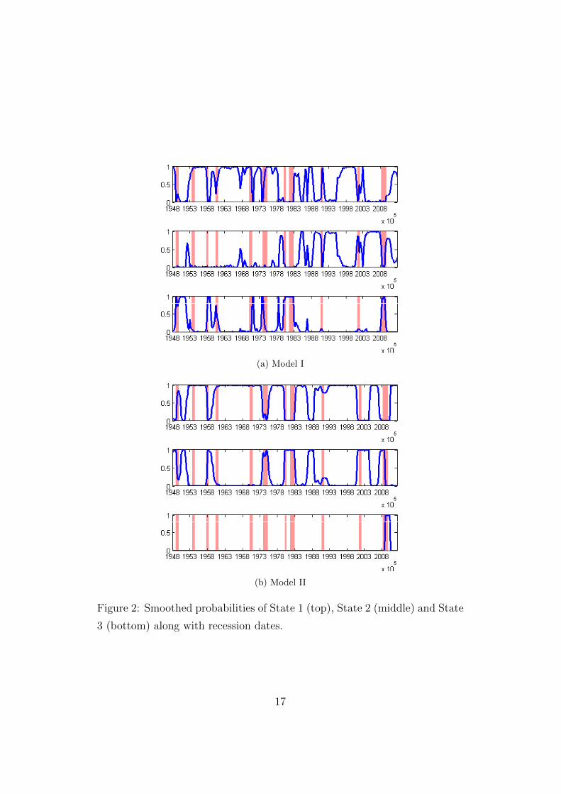
with each state can be seen in Figure 2, where smoothed state probabilities

are plotted. In both models the first state captures mostly periods not asso-

ciated with recessions while most recession periods are associated with States

2 and 3 which explains the higher volatility in these states. In fact, State 3 of

Model II captures the last recession only, where apparently the volatility in

our series was particularly high. Given the differences in volatility across the

states, it makes sense to use the heteroskedasticity for identification purposes.

Since our approach relies on the covariance decomposition (6), the first

question is whether such a decomposition is in line with the data. Using the

likelihood ratio test from Lanne et al. (2010) for checking the decomposition

gives the p-values in Table 1. They are both greater than the 5% critical

level. Hence, we proceed by assuming that the data do not object to the

decomposition in either of the two models. The next step is to check whether

the decomposition can be used for identification of structural shocks.

To see whether the covariance decomposition in (6) is unique, we have to

check the diagonal elements of the Λm matrices, that is, the relative variances,

relative to State 1, for sufficient heterogeneity. The estimates are presented

in Table 2. Even when accounting for the estimation uncertainty reflected

in the standard errors, the estimated λmk are indeed quite heterogeneous.

Hence, testing the identification conditions formally is plausible.

As noted in Section 3.1, uniqueness of the B matrix in (6) up to sign is

ensured if all pairwise diagonal elements, λm,k,m = 2, . . . ,M, k = 1, . . . , K,

are distinct in at least one Λm,m = 2, . . . ,M , matrix for a given pair. In

other words, for our specific three-state models we have to check the null

hypotheses given in Table 3. This can be done by a simple Wald test. Under

standard assumptions the test distribution is asymptotically χ2 with the

number of degrees of freedom equal to the number of joint hypotheses tested.

The relevant null hypotheses along with p-values of Wald tests are given in

Table 3. They are all found to be rejected for Model I at conventional

16

(a) Model I

(b) Model II

Figure 2: Smoothed probabilities of State 1 (top), State 2 (middle) and State

3 (bottom) along with recession dates.

17

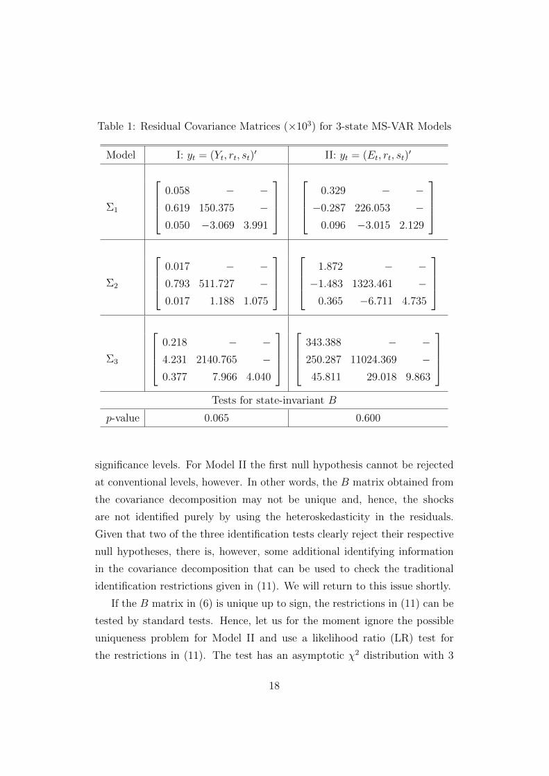
Table 1: Residual Covariance Matrices (×103) for 3-state MS-VAR Models

Model I: yt = (Yt, rt, st)′ II: yt = (Et, rt, st)

′

Σ1

0.058 − −0.619 150.375 −0.050 −3.069 3.991

0.329 − −−0.287 226.053 −

0.096 −3.015 2.129

Σ2

0.017 − −0.793 511.727 −0.017 1.188 1.075

1.872 − −−1.483 1323.461 −

0.365 −6.711 4.735

Σ3

0.218 − −4.231 2140.765 −0.377 7.966 4.040

343.388 − −250.287 11024.369 −45.811 29.018 9.863

Tests for state-invariant B

p-value 0.065 0.600

significance levels. For Model II the first null hypothesis cannot be rejected

at conventional levels, however. In other words, the B matrix obtained from

the covariance decomposition may not be unique and, hence, the shocks

are not identified purely by using the heteroskedasticity in the residuals.

Given that two of the three identification tests clearly reject their respective

null hypotheses, there is, however, some additional identifying information

in the covariance decomposition that can be used to check the traditional

identification restrictions given in (11). We will return to this issue shortly.

If the B matrix in (6) is unique up to sign, the restrictions in (11) can be

tested by standard tests. Hence, let us for the moment ignore the possible

uniqueness problem for Model II and use a likelihood ratio (LR) test for

the restrictions in (11). The test has an asymptotic χ2 distribution with 3

18

Table 2: Estimates and Standard Errors of Relative Variances of MS-VAR

Models

Model I: yt = (Yt, rt, st)′ II: yt = (Et, rt, st)

′

Parameter estimate standard error estimate standard error

λ21 0.267 0.094 5.702 1.251

λ22 0.277 0.089 5.925 1.311

λ23 3.564 1.051 2.215 0.518

λ31 0.845 0.252 1050.264 620.878

λ32 3.777 1.004 48.731 36.057

λ33 14.878 4.117 1.778 1.150

Table 3: p-values of Wald tests of Identification Conditions

H0 Model I Model II

λ21 = λ22, λ31 = λ32 0.011 0.263

λ21 = λ23, λ31 = λ33 0.000 0.014

λ22 = λ23, λ32 = λ33 0.001 0.016

degrees of freedom since in each case there are 3 independent restrictions if B

is unique. The p-values of the tests based on χ2(3) distributions are given in

Table 4. Using standard significance levels, Model I cannot be rejected given

a p-value of roughly 20%. On the other hand, Model II is clearly rejected

at conventional significance levels. The latter result means that even though

the B matrix is not unique, by using the heteroskedasticity of the residuals,

the restrictions imposed are sufficient to reject the identification scheme for

Model II. Note that nonuniqueness of B may imply that the actual number

of degrees of freedom of the χ2 distribution is lower than 3. Hence, the

actual p-value may be even smaller than the one in Table 4. Thus, using the

heteroskedasticity device, we can clearly reject the identification scheme for

Model II and find some support for Model I.

19

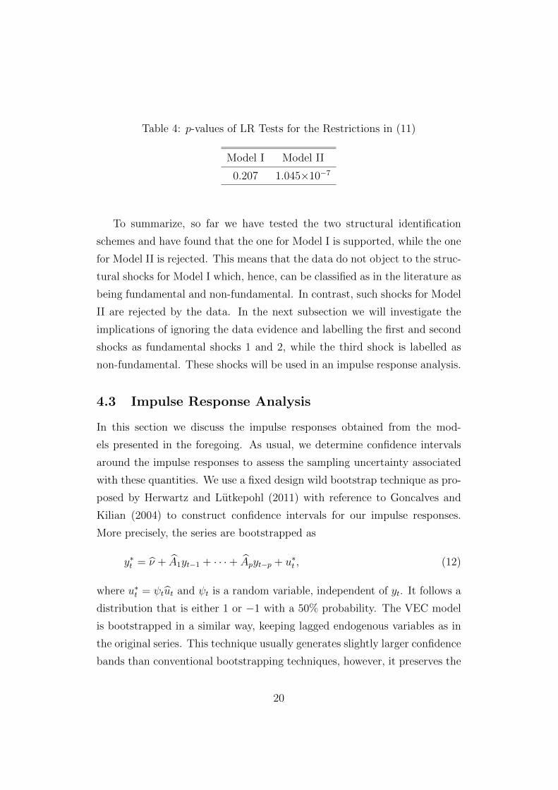
Table 4: p-values of LR Tests for the Restrictions in (11)

Model I Model II

0.207 1.045×10−7

To summarize, so far we have tested the two structural identification

schemes and have found that the one for Model I is supported, while the one

for Model II is rejected. This means that the data do not object to the struc-

tural shocks for Model I which, hence, can be classified as in the literature as

being fundamental and non-fundamental. In contrast, such shocks for Model

II are rejected by the data. In the next subsection we will investigate the

implications of ignoring the data evidence and labelling the first and second

shocks as fundamental shocks 1 and 2, while the third shock is labelled as

non-fundamental. These shocks will be used in an impulse response analysis.

4.3 Impulse Response Analysis

In this section we discuss the impulse responses obtained from the mod-

els presented in the foregoing. As usual, we determine confidence intervals

around the impulse responses to assess the sampling uncertainty associated

with these quantities. We use a fixed design wild bootstrap technique as pro-

posed by Herwartz and Lutkepohl (2011) with reference to Goncalves and

Kilian (2004) to construct confidence intervals for our impulse responses.

More precisely, the series are bootstrapped as

y∗t = ν + A1yt−1 + · · ·+ Apyt−p + u∗t , (12)

where u∗t = ψtut and ψt is a random variable, independent of yt. It follows a

distribution that is either 1 or −1 with a 50% probability. The VEC model

is bootstrapped in a similar way, keeping lagged endogenous variables as in

the original series. This technique usually generates slightly larger confidence

bands than conventional bootstrapping techniques, however, it preserves the

20

heteroskedastic properties of the residuals. The hats in (12) denote estimated

coefficients.

Impulse responses for Models I and II are depicted in Figure 3. Confi-

dence bands show the 95% and 68% individual bootstrap confidence intervals

around the impulse responses. As was noted, for convenience, the shocks in

both models are labelled in the same way, even though the identification

scheme is rejected for Model II. Since the investigation is focused on stock

price fundamentals we are particularly interested in the response of stock

prices to the fundamental shocks.

For Model I, the first fundamental shock has a positive and permanent

impact on stock prices. Even the 95% confidence intervals are well away

from the zero line so that a significant impact of the first fundamental shock

on stock prices is diagnosed. For Model II, the impulse response function of

stock prices to the first fundamental shock is still positive. Now the zero line

is within the confidence band when a 95% level is used and it is at the lower

bound when the 68% level is considered. It should be noted that this result

is not merely due to using the fixed design wild bootstrap method. In fact,

if the series is bootstrapped in a conventional way, the response is still not

significantly away from zero at the 95% level.4 Moreover, in Figure 3 it is

seen that the second fundamental shock does not have a significant impact

in Model II even if a 68% confidence level is used. Hence, if Model II is used

for investigating the impact of fundamental shocks on stock prices, one may

be led to conclude that fundamental shocks have little impact and that stock

prices are mainly driven by speculation.

Thus, Models I and II lead to opposite conclusions and in a conventional

analysis there is no statistical procedure to discriminate between them. In

contrast, using the additional information from the changes in volatility al-

lows us to discriminate between the two models. Clearly, Model II is rejected

4We have not explored the possibility to reduce the confidence bands by reduction

techniques as discussed by Lutkepohl (2013b) because we are interested in the results

obtained with the standard approach.

21

0 5 10 150

0.01

Fundamental Shock 1

Rea

l GD

P

0 5 10 150

1

2

x 10−3

Fundamental Shock 2

0 5 10 15

−4

−2

0x 10

−3Non−fundamental Shock

0 5 10 15

−0.10

0.10.20.3

Rea

l Int

eres

t Rat

es

0 5 10 150

0.5

0 5 10 15−0.15−0.1

−0.050

0.05

0 5 10 150

0.05

Rea

l Sto

ck P

rices

0 5 10 15−0.03−0.02−0.01

00.01

0 5 10 150

0.05

(a) Model I

0 5 10 15

0

0.1

0.2

Fundamental Shock 1

Rea

l Ear

ning

s

0 5 10 15

−0.050

0.050.1

Fundamental Shock 2

0 5 10 15

−0.1

0

0.1

Non−fundamental Shock

0 5 10 15

−0.5

0

0.5

Rea

l Int

eres

t Rat

es

0 5 10 150

0.20.40.60.8

0 5 10 15

−0.5

0

0.5

0 5 10 15−0.05

0

0.05

Rea

l Sto

ck P

rices

0 5 10 15

−0.05

0

0.05

0 5 10 15

00.020.040.06

(b) Model II

Figure 3: Impulse responses for models I and II with 95 and 68 percentile

confidence intervals according to the fixed design wild bootstrap method.

22

by the data and, hence, we have a basis for deciding between the two models.

This illustrates the virtue of using heteroskedasticity for testing identifying

restrictions.

5 Conclusions

In this study we have considered long-run restrictions for identifying struc-

tural shocks in a VAR model. We have reviewed different approaches for

checking restrictions that are just-identifying in a conventional setting by

utilizing heteroskedasticity in the residuals, with special emphasis on the

case where integrated and cointegrated variables are included in the models.

The three main approaches for modelling changes in volatility that have been

used in this context are exogenously generated changes in volatility, endoge-

nous changes driven by a Markov process and volatility changes generated

by MGARCH processes. We have briefly discussed the related techniques for

identifying the shocks and, in particular, we have discussed how the addi-

tional identifying information obtained from heteroskedasticity can be used

in a structural analysis.

To illustrate the identification through heteroskedasticity technique, two

models investigating stock price fundamentals are considered. Both are

trivarite models, based on the dividend discount model (DDM) and have

widely been used in the empirical time series literature. The models labelled

as I and II have different proxies of real economic activity. Model I uses real

GDP, while Model II uses real earnings, the other variables being real interest

rates and real stock prices ordered in that way. It is shown how the changes

in volatility found in these models can be used for testing conventional iden-

tifying restrictions. Since the conventional restrictions are just-identifying,

they cannot be formally tested in a standard setup and it turns out that

the two models lead to quite different conclusions regarding the impact of

fundamental shocks on stock prices. Model I indicates that they may have

an important impact even in the long-run while no significant effect is found

23

in Model II. Using the changes in volatility allows us to discriminate between

the two models and it is shown that Model II is rejected by the data whereas

support is found for Model I. In other words, support is found for the con-

clusion that stock prices are at least to some extent driven by fundamental

shocks.

References

Binswanger, M. (2004). How do stock prices respond to fundamental shocks?,

Finance Research Letters 1(2): 90–99.

Blanchard, O. and Quah, D. (1989). The dynamic effects of aggregate de-

mand and supply disturbances, American Economic Review 79: 655–

673.

Bouakez, H. and Normandin, M. (2010). Fluctuations in the foreign ex-

change market: How important are monetary policy shocks?, Journal

of International Economics 81: 139–153.

Ehrmann, M., Fratzscher, M. and Rigobon, R. (2011). Stocks, bonds, money

markets and exchange rates: Measuring international financial trans-

mission, Journal of Applied Econometrics 26: 948–974.

Fisher, L. A. and Huh, H.-S. (2014). Identification methods in vector-error

correction models: Equivalence results, Journal of Economic Surveys

28: 1–16.

Fisher, L. A., Huh, H.-S. and Summers, P. M. (2000). Structural identifica-

tion of permanent shocks in VEC models: A generalization, Journal of

Macroeconomics 22: 53–68.

Garcia, R. (1998). Asymptotic null distribution of the likelihood ratio test in

Markov switching models, International Economic Review 39: 763–788.

24

Goncalves, S. and Kilian, L. (2004). Bootstrapping autoregressions with con-

ditional heteroskedasticity of unknown form, Journal of Econometrics

123(1): 89–120.

Gonzalo, J. and Ng, S. (2001). A systematic framework for analyzing the dy-

namic effects of permanent and transitory shocks, Journal of Economic

Dynamics and Control 25: 1527–1546.

Hansen, B. E. (1992). The likelihood ratio test under nonstandard condi-

tions: Testing the Markov switching model of GNP, Journal of Applied

Econometrics 7: 61–82 (erratum: 11, 195–198).

Herwartz, H. and Lutkepohl, H. (2011). Structural vector autoregressions

with Markov switching: Combining conventional with statistical identi-

fication of shocks, Working Paper series, EUI, Florence.

Jean, R. and Eldomiaty, T. (2010). How do stock prices respond to funda-

mental shocks in the case of the United States? Evidence from NASDAQ

and DJIA, The Quarterly Review of Economics and Finance 50(3): 310–

322.

Johansen, S. (1995). Likelihood-based Inference in Cointegrated Vector Au-

toregressive Models, Oxford University Press, Oxford.

King, R. G., Plosser, C. I., Stock, J. H. and Watson, M. W. (1991). Stochastic

trends and economic fluctuations, American Economic Review 81: 819–

840.

Krolzig, H.-M. (1997). Markov-Switching Vector Autoregressions: Mod-

elling, Statistical Inference, and Application to Business Cycle Analysis,

Springer-Verlag, Berlin.

Lanne, M. and Lutkepohl, H. (2008a). Identifying monetary policy shocks via

changes in volatility, Journal of Money, Credit and Banking 40: 1131–

1149.

25

Lanne, M. and Lutkepohl, H. (2008b). A statistical comparison of alternative

identification schemes for monetary policy shocks, European University

Institute, Florence, mimeo.

Lanne, M. and Lutkepohl, H. (2010). Structural vector autoregressions

with nonnormal residuals, Journal of Business & Economic Statistics

28: 159–168.

Lanne, M., Lutkepohl, H. and Maciejowska, K. (2010). Structural vector

autoregressions with Markov switching, Journal of Economic Dynamics

and Control 34: 121–131.

Lee, B. (1995). Fundamentals and bubbles in asset prices: Evidence from us

and japanese asset prices, Asia-Pacific Financial Markets 2(2): 89–122.

Lutkepohl, H. (2005). New Introduction to Multiple Time Series Analysis,

Springer-Verlag, Berlin.

Lutkepohl, H. (2013a). Identifying structural vector autoregressions via

changes in volatility, Advances in Econometrics 32: 169–203.

Lutkepohl, H. (2013b). Reducing confidence bands for simulated impulse

responses, Statistical Papers 54: 1131–1145.

Lutkepohl, H. and Netsunajev, A. (2013). Disentangling demand and sup-

ply shocks in the crude oil market: How to check sign restrictions in

structural VARs, Journal of Applied Econometrics forthcoming.

Netsunajev, A. (2013). Reaction to technology shocks in Markov-switching

structural VARs: Identification via heteroskedasticity, Journal of

Macroeconomics 36: 51–62.

Normandin, M. and Phaneuf, L. (2004). Monetary policy shocks: Testing

identification conditions under time-varying conditional volatility, Jour-

nal of Monetary Economics 51: 1217–1243.

26

Pagan, A. R. and Pesaran, M. H. (2008). Econometric analysis of structural

systems with permanent and transitory shocks, Journal of Economic

Dynamics and Control 32: 3376–3395.

Psaradakis, Z. and Spagnolo, N. (2003). On the determination of the number

of regimes in Markov-switching autoregressive models, Journal of Time

Series Analysis 24: 237–252.

Psaradakis, Z. and Spagnolo, N. (2006). Joint determination of the state di-

mension and autoregressive order for models with Markov regime switch-

ing, Journal of Time Series Analysis 27: 753–766.

Rapach, D. (2001). Macro shocks and real stock prices, Journal of Economics

and Business 53(1): 5–26.

Rigobon, R. (2003). Identification through heteroskedasticity, Review of Eco-

nomics and Statistics 85: 777–792.

Rigobon, R. and Sack, B. (2003). Measuring the reaction of monetary policy

to the stock market, Quarterly Journal of Economics 118: 639–669.

Rigobon, R. and Sack, B. (2004). The impact of monetary policy on asset

prices, Journal of Monetary Economics 51: 1553–1575.

Rubio-Ramirez, J. F., Waggoner, D. and Zha, T. (2005). Markov-switching

structural vector autoregressions: Theory and applications, Discussion

Paper, Federal Reserve Bank of Atlanta.

Sentana, E. and Fiorentini, G. (2001). Identification, estimation and testing

of conditionally heteroskedastic factor models, Journal of Econometrics

102: 143–164.

Sims, C. A., Waggoner, D. F. and Zha, T. (2008). Methods for inference

in large multiple-equation Markov-switching models, Journal of Econo-

metrics 146: 255–274.

27

Sims, C. A. and Zha, T. (2006). Were there regime switches in U.S. monetary

policy?, American Economic Review 96: 54–81.

Strohsal, T. and Weber, E. (2012). The signal of volatility, Discussion Paper

2012-043, Humboldt University Berlin, SFB 649.

van der Weide, R. (2002). GO-GARCH: A multivariate generalized orthog-

onal GARCH model, Journal of Applied Econometrics 17: 549–564.

Velinov, A. S. (2013). Can stock price fundamentals really be captured? Us-

ing Markov switching in heteroskedasticity models to test identification

restrictions, Discussion Paper 1350, DIW Berlin.

Vrontos, I. D., Dellaportas, P. and Politis, D. N. (2003). A full-factor multi-

variate GARCH model, Econometrics Journal 6: 312–334.

Weber, E. (2010). Structural conditional correlation, Journal of Financial

Econometrics 8: 392–407.

28

SFB 649 Discussion Paper Series 2014

For a complete list of Discussion Papers published by the SFB 649,

please visit http://sfb649.wiwi.hu-berlin.de.

001 "Principal Component Analysis in an Asymmetric Norm" by Ngoc Mai

Tran, Maria Osipenko and Wolfgang Karl Härdle, January 2014.

002 "A Simultaneous Confidence Corridor for Varying Coefficient Regression

with Sparse Functional Data" by Lijie Gu, Li Wang, Wolfgang Karl Härdle

and Lijian Yang, January 2014.

003 "An Extended Single Index Model with Missing Response at Random" by

Qihua Wang, Tao Zhang, Wolfgang Karl Härdle, January 2014.

004 "Structural Vector Autoregressive Analysis in a Data Rich Environment:

A Survey" by Helmut Lütkepohl, January 2014.

005 "Functional stable limit theorems for efficient spectral covolatility

estimators" by Randolf Altmeyer and Markus Bibinger, January 2014.

006 "A consistent two-factor model for pricing temperature derivatives" by

Andreas Groll, Brenda López-Cabrera and Thilo Meyer-Brandis, January

2014.

007 "Confidence Bands for Impulse Responses: Bonferroni versus Wald" by

Helmut Lütkepohl, Anna Staszewska-Bystrova and Peter Winker, January

2014.

008 "Simultaneous Confidence Corridors and Variable Selection for

Generalized Additive Models" by Shuzhuan Zheng, Rong Liu, Lijian Yang

and Wolfgang Karl Härdle, January 2014.

009 "Structural Vector Autoregressions: Checking Identifying Long-run

Restrictions via Heteroskedasticity" by Helmut Lütkepohl and Anton

Velinov, January 2014.

SFB 649, Spandauer Straße 1, D-10178 Berlin

http://sfb649.wiwi.hu-berlin.de

This research was supported by the Deutsche

Forschungsgemeinschaft through the SFB 649 "Economic Risk".