THE UNIVERSITY OF CALGARY

Interactive Modeling with Implicit Surfaces

by

Ryan Schmidt

A THESIS

SUBMITTED TO THE FACULTY OF GRADUATE STUDIES

IN PARTIAL FULFILLMENT OF THE REQUIREMENTS FOR THE

DEGREE OF MASTER OF SCIENCE

DEPARTMENT OF COMPUTER SCIENCE

CALGARY, ALBERTA

August, 2006

c© Ryan Schmidt 2006

THE UNIVERSITY OF CALGARY

FACULTY OF GRADUATE STUDIES

The undersigned certify that they have read, and recommend to the Faculty of Graduate Studiesfor acceptance, a thesis entitled “Interactive Modeling with Implicit Surfaces” submitted by RyanSchmidt in partial fulfillment of the requirements for the degree of MASTER OF SCIENCE.

Supervisor,Dr. Brian WyvillDepartment of Computer Science

Dr. Faramarz SamavatiDepartment of Computer Science

Dr. Mario Costa SousaDepartment of Computer Science

External Examiner,Dr. Neil DuncanDepartment of Civil Engineering

Date

ii

Abstract

Interactive tools for shape modeling with hierarchical implicit surfaces have been limited bothby the high computational cost of visualization, and the lack of techniques for direct surfacemanipulation. To address the visualization issue, Hierarchical Spatial Caching is developed.This novel technique combines caching and spatial approximation to accelerate queries of thefunctional model tree. By reducing the cost of evaluating cached branches from O(N) to O(1), anorder-of-magnitude improvement in visualization speed is realized. A new implicit sweep surfaceformulation which supports direct manipulation of the sweep profile is also developed, providing apowerful and flexible free-form implicit primitive. These new techniques form the core of a proof-of-concept interactive modeling environment, called ShapeShop. ShapeShop provides a level ofinteractive control over hierarchical implicit models which has not been previously available. Asurvey of current techniques for shape modeling with implicit surfaces is also provided.

iii

Acknowledgements

Where does one begin? Clearly, there is Ailidh. Thank you for your patience (particularly atpaper deadlines), encouragement, understanding, and support. And thank you for listening.Without you, this whole thing simply wouldn’t have happened.

Of course, there is Brian Wyvill, with his subtle pushes at opportune moments. Thanks forall your encouragement, advice, and willingness to let me figure things out for myself (hopefullyI wasn’t too much trouble). Oh, and thanks for the second chance. I also have to thank FrankMaurer, for introducing me to the research game (Sorry I skipped out on you for graphics -but then, you always knew I was a hacker). There have been many other professors who havemade an impact on my work. Mario Costa Sousa, Faramarz Samavati, Przemek Prusinkiewicz,Jon Rokne, Ehud Sharlin, Sheelagh Carpendale, Saul Greenberg, Richard Lobb, and JoaquimJorge - whether technical assistance, encouragement, or simply stimulating conversation, youhave all helped me along the way. Also thanks to Eric Galin, your help with the SMI paper wasinvaluable, and Neil Duncan who gave me a glimpse of life beyond computer graphics.

There have been many students who have helped me along the way, far too many to listhere. Hopefully, you know who you are. First and foremost, thanks to all the members of theGraphics Jungle and Interactions Lab at the University of Calgary. In particular, Pauline Jepp,Tobias Isenberg, Michael Boyle, Callum Galbraith, Kevin Foster, Anand Agarawala, StaceyScott, Mark Hancock, Torre Zuk, Mark Fox, Chester Fitchett, Robson Lemos, Brendan Lane,Carla Davidson, Lars Muenderman, Marilyn Powers, and Peter MacMurchy. Thank you for yourassistance, encouragement, conversation and friendship. Also thanks to the many great people Ihave met at conferences, particularly Tamy Boubekeur, Patricio Simari, Nisha Sudarsanam, andLoic Barthe. And, of course, my agent, Rob Leclerc, who got me into graphics in the first place,and is always willing to challenge my thinking. The support staff at the University of Calgaryhave also been fantastic, particularly Wayne Pearson, Camille Sinanan, and the front-office staff.

Finally, my friends and family have been a source of never-ending support. The residents ofthe Sugar Shack made a significant impact on my work (and mental well-being), as have all myother house-mates along the way. Thanks to my parents, for their support (both financial andotherwise), and to Kyle and Mandy, who each keep me on my toes in their own way.

iv

Table of Contents

Approval Page ii

Abstract iii

Acknowledgements iv

Table of Contents v

1 Introduction 1

1.1 Goals . . . . . . . . . . . . . . . . . . . . . . . . . . . . . . . . . . . . . . . . . . . 31.2 Contributions . . . . . . . . . . . . . . . . . . . . . . . . . . . . . . . . . . . . . . 41.3 Scope . . . . . . . . . . . . . . . . . . . . . . . . . . . . . . . . . . . . . . . . . . 51.4 Summary . . . . . . . . . . . . . . . . . . . . . . . . . . . . . . . . . . . . . . . . 5

2 Shape Modeling with Implicit Surfaces 7

2.1 Implicit Surfaces . . . . . . . . . . . . . . . . . . . . . . . . . . . . . . . . . . . . 72.2 Implicit Volumes . . . . . . . . . . . . . . . . . . . . . . . . . . . . . . . . . . . . 82.3 Solid Modeling . . . . . . . . . . . . . . . . . . . . . . . . . . . . . . . . . . . . . 92.4 Blending . . . . . . . . . . . . . . . . . . . . . . . . . . . . . . . . . . . . . . . . . 92.5 Bounded Fields . . . . . . . . . . . . . . . . . . . . . . . . . . . . . . . . . . . . . 112.6 Continuity and Manifolds . . . . . . . . . . . . . . . . . . . . . . . . . . . . . . . 122.7 C1 Continuity and The Gradient . . . . . . . . . . . . . . . . . . . . . . . . . . . 142.8 Higher Order Continuity and Perceptual Discontinuities . . . . . . . . . . . . . . . 152.9 Field Normalization and Surface Convergence . . . . . . . . . . . . . . . . . . . . 16

2.9.1 Analyzing Field Normalization Error . . . . . . . . . . . . . . . . . . . . . 172.10 The Scaling Problem . . . . . . . . . . . . . . . . . . . . . . . . . . . . . . . . . . 182.11 Chapter Summary . . . . . . . . . . . . . . . . . . . . . . . . . . . . . . . . . . . 20

3 A Taxonomy of Implicit Surfaces 21

3.1 Introduction . . . . . . . . . . . . . . . . . . . . . . . . . . . . . . . . . . . . . . . 213.2 Classification Properties . . . . . . . . . . . . . . . . . . . . . . . . . . . . . . . . 223.3 Constructive Modeling Frameworks . . . . . . . . . . . . . . . . . . . . . . . . . . 23

3.3.1 Distance Fields, R-Functions, and F-Reps . . . . . . . . . . . . . . . . . . 233.3.2 BlobTree Modeling . . . . . . . . . . . . . . . . . . . . . . . . . . . . . . . 243.3.3 Convolution Surfaces . . . . . . . . . . . . . . . . . . . . . . . . . . . . . . 25

3.4 Uniformly-Sampled Discrete Volume Datasets . . . . . . . . . . . . . . . . . . . . 253.4.1 Adaptive Distance Fields . . . . . . . . . . . . . . . . . . . . . . . . . . . . 26

3.5 Point-Set Interpolation Schemes . . . . . . . . . . . . . . . . . . . . . . . . . . . . 263.5.1 Variational Implicit Surfaces . . . . . . . . . . . . . . . . . . . . . . . . . . 263.5.2 Compactly-Supported Variational Implicit Surfaces . . . . . . . . . . . . . 27

v

3.5.3 Multi-level Partition of Unity Implicits . . . . . . . . . . . . . . . . . . . . 273.5.4 Implicit Moving Least-Squares . . . . . . . . . . . . . . . . . . . . . . . . . 28

3.6 Classification Summary . . . . . . . . . . . . . . . . . . . . . . . . . . . . . . . . . 283.7 Selecting a Modeling Framework . . . . . . . . . . . . . . . . . . . . . . . . . . . . 283.8 Chapter Summary . . . . . . . . . . . . . . . . . . . . . . . . . . . . . . . . . . . 30

4 Hierarchical Spatial Caching 31

4.1 The Interactive Visualization Problem . . . . . . . . . . . . . . . . . . . . . . . . 314.2 Problem Analysis and Solution Overview . . . . . . . . . . . . . . . . . . . . . . . 324.3 Previous Caching and Approximation Schemes . . . . . . . . . . . . . . . . . . . . 334.4 Hierarchical Spatial Caching . . . . . . . . . . . . . . . . . . . . . . . . . . . . . . 354.5 Hierarchical Spatial Caching Implementation Issues . . . . . . . . . . . . . . . . . 374.6 Sampling and Reconstruction . . . . . . . . . . . . . . . . . . . . . . . . . . . . . 394.7 A Sample Spatial Caching Implementation . . . . . . . . . . . . . . . . . . . . . . 41

4.7.1 Dynamic Grid Resolution . . . . . . . . . . . . . . . . . . . . . . . . . . . 414.7.2 Cache Coordinate System . . . . . . . . . . . . . . . . . . . . . . . . . . . 424.7.3 Blocked Memory Allocation . . . . . . . . . . . . . . . . . . . . . . . . . . 424.7.4 Last-Access Caching . . . . . . . . . . . . . . . . . . . . . . . . . . . . . . 434.7.5 Dynamic Cache Placement . . . . . . . . . . . . . . . . . . . . . . . . . . . 43

4.8 Results and Analysis . . . . . . . . . . . . . . . . . . . . . . . . . . . . . . . . . . 444.8.1 Static Polygonization Time . . . . . . . . . . . . . . . . . . . . . . . . . . 454.8.2 Interactive Polygonization Time . . . . . . . . . . . . . . . . . . . . . . . . 464.8.3 Local Update Polygonization . . . . . . . . . . . . . . . . . . . . . . . . . 474.8.4 Approximation Error . . . . . . . . . . . . . . . . . . . . . . . . . . . . . . 48

4.9 Spatial Caching with Adaptive Distance Fields . . . . . . . . . . . . . . . . . . . . 504.9.1 Octree Subdivision . . . . . . . . . . . . . . . . . . . . . . . . . . . . . . . 514.9.2 Dynamic Construction . . . . . . . . . . . . . . . . . . . . . . . . . . . . . 514.9.3 Sampling Cost . . . . . . . . . . . . . . . . . . . . . . . . . . . . . . . . . . 534.9.4 Continuity . . . . . . . . . . . . . . . . . . . . . . . . . . . . . . . . . . . . 54

4.10 Chapter Summary . . . . . . . . . . . . . . . . . . . . . . . . . . . . . . . . . . . 54

5 Implicit Sweep Surfaces 56

5.1 Implicit Sweep Surfaces . . . . . . . . . . . . . . . . . . . . . . . . . . . . . . . . . 565.2 Previous Approaches . . . . . . . . . . . . . . . . . . . . . . . . . . . . . . . . . . 575.3 2D Implicit Sweep Templates . . . . . . . . . . . . . . . . . . . . . . . . . . . . . 60

5.3.1 Bounding Distance Fields . . . . . . . . . . . . . . . . . . . . . . . . . . . 605.3.2 C2 Distance Field Approximation . . . . . . . . . . . . . . . . . . . . . . . 605.3.3 Sharp Features . . . . . . . . . . . . . . . . . . . . . . . . . . . . . . . . . 625.3.4 Analysis . . . . . . . . . . . . . . . . . . . . . . . . . . . . . . . . . . . . . 64

5.4 Sweep Primitives . . . . . . . . . . . . . . . . . . . . . . . . . . . . . . . . . . . . 665.4.1 Linear Trajectory . . . . . . . . . . . . . . . . . . . . . . . . . . . . . . . . 675.4.2 Circular Trajectory . . . . . . . . . . . . . . . . . . . . . . . . . . . . . . . 695.4.3 Cubic Bezier Trajectory . . . . . . . . . . . . . . . . . . . . . . . . . . . . 70

vi

5.5 Self-Intersection . . . . . . . . . . . . . . . . . . . . . . . . . . . . . . . . . . . . . 715.6 Discrete Sweep Templates . . . . . . . . . . . . . . . . . . . . . . . . . . . . . . . 725.7 Parametric to Implicit Sweep Conversion . . . . . . . . . . . . . . . . . . . . . . . 725.8 Surface Reconstruction from Parallel Contours . . . . . . . . . . . . . . . . . . . . 735.9 Chapter Summary . . . . . . . . . . . . . . . . . . . . . . . . . . . . . . . . . . . 74

6 ShapeShop: A Proof-of-Concept 76

6.1 Interactive Implicit Modeling Systems . . . . . . . . . . . . . . . . . . . . . . . . . 766.2 Overview . . . . . . . . . . . . . . . . . . . . . . . . . . . . . . . . . . . . . . . . . 776.3 ShapeShop Interface . . . . . . . . . . . . . . . . . . . . . . . . . . . . . . . . . . 786.4 Sketch-Based Modeling Operations . . . . . . . . . . . . . . . . . . . . . . . . . . 786.5 Node Selection and BlobTree Traversal . . . . . . . . . . . . . . . . . . . . . . . . 826.6 BlobTree Visualization . . . . . . . . . . . . . . . . . . . . . . . . . . . . . . . . . 826.7 BlobTree Implementation Details . . . . . . . . . . . . . . . . . . . . . . . . . . . 836.8 Limitations and Future Work . . . . . . . . . . . . . . . . . . . . . . . . . . . . . 846.9 Chapter Summary . . . . . . . . . . . . . . . . . . . . . . . . . . . . . . . . . . . 85

7 Results and Conclusion 86

7.1 Results . . . . . . . . . . . . . . . . . . . . . . . . . . . . . . . . . . . . . . . . . . 867.1.1 Interactive Assembly . . . . . . . . . . . . . . . . . . . . . . . . . . . . . . 877.1.2 Character Modeling . . . . . . . . . . . . . . . . . . . . . . . . . . . . . . . 887.1.3 Mechanical Parts . . . . . . . . . . . . . . . . . . . . . . . . . . . . . . . . 907.1.4 Biological Modeling . . . . . . . . . . . . . . . . . . . . . . . . . . . . . . . 927.1.5 Design Iteration . . . . . . . . . . . . . . . . . . . . . . . . . . . . . . . . . 937.1.6 Observations . . . . . . . . . . . . . . . . . . . . . . . . . . . . . . . . . . 93

7.2 Future Work . . . . . . . . . . . . . . . . . . . . . . . . . . . . . . . . . . . . . . . 937.3 Conclusion . . . . . . . . . . . . . . . . . . . . . . . . . . . . . . . . . . . . . . . . 95

A Linear and Quadratic Reconstruction Filters 96

A.1 Tri-Linear Reconstruction Filter . . . . . . . . . . . . . . . . . . . . . . . . . . . . 96A.2 Tri-Quadratic Reconstruction Filter . . . . . . . . . . . . . . . . . . . . . . . . . . 96

B Variational Implicit Curves 98

C Normalized Implicit Polygons 99

Bibliography 100

vii

Chapter 1

Introduction

Interactive shape modeling is a wide-ranging topic with a history reaching back to the earliestdays of interactive computing. For example, one of the first works in computer graphics was theSketchPad system, the subject of Ivan Sutherland’s dissertation in 1963 [111]. Sketchpad, one ofthe pioneering works in Computer-Aided Design [47], was essentially a 2D modeling system. Theinteraction techniques introduced in Sketchpad have heavily influenced the design of modern 3Dmodeling interfaces.

One issue inherent in any 3D modeling system is how to represent shapes. The commonshape representation techniques have varying strengths and weaknesses with respect to differentinteraction techniques. For example, parametric spline patches can be easily sculpted by manip-ulating their control points, but applying similar deformations to a sphere defined as an implicitsurface is quite difficult. In contrast, creating a blend surface between two solid objects repre-sented using parametric patches can be extremely difficult, while blending two implicitly-definedsolid objects is nearly trivial. Modern shape modeling interfaces are heavily influenced by thesedifferences. In fact, most commercial modeling tools are identified by how they represent shapes -some are “parametric” or “patch-based” modelers, while others are “mesh editors”, “subdivisionsystems”, “volume sculpting tools”, and so on. The design of these interfaces is driven by whatkinds of operations the underlying shape representation easily supports.

In this respect, implicit surfaces are simply another option in the library of shape represen-tation techniques. However, implicit surfaces have some tangible benefits in the domain of solidmodeling [85, 86], which is a subset of shape modeling explicitly concerned with the representa-tion of 3D models which are in a sense “isomorphic” to some real-world shape. Not all modelsused in computer graphics are solid models - for example, pieces of cloth are often representedby infinitely-thin triangle meshes. However, this is usually done for efficiency, and solid modelsarguably would be more accurate since all physical objects have a volume (and in the case ofdeformable surfaces, are known to produce more realistic simulations [31]). With the increasingavailability of rapid prototyping machines, also known as “3D printers”, interest in solid model-ing is growing, and with it the need for solid modeling interfaces. This work will focus on suchinterfaces.

Solids can be represented in a variety of ways. The most common approach in computergraphics is to represent a solid by describing it’s boundary - the infinitely-thin surface thatmakes up the exterior of the solid. Complex boundaries are usually described by combining aset of boundary patches. The union of the boundary patches encloses some 3D space, which isthe volume of the solid. Hence, the boundary of a cube could be 6 square patches. This typeof solid is often referred to as a boundary represention or B-Rep [85, 86]. Common techniquesused to define boundary patches include parametric spline surfaces, triangle meshes, subdivisionmeshes, and analytic surfaces such as conics.

The alternative to boundary representations are volumetric representations, where the solidis represented directly. Volumetric representations are based on the concept of spatial enumer-

1

2

ation, where each point is classified as being inside or outside the volume. Note that whileany volumetric representation can be considered a boundary representation (since the surface ofthe volume is it’s boundary), the reverse is not true. The fundamental distinction is that withvolume representations, any 3D point can always be classified as inside or outside the surface.This is known as the point classification test, and is inherently related to the notion of validityof solid models. With B-Reps, it is possible to have a hole or “crack” between two boundarypatches, or to have two boundary patches intersect. In these cases, “inside” and “outside” arenot mathematically well-defined, and hence (for the purposes of representing a solid) the modelis invalid [85].

With respect to validity in solid modeling, volumetric models have clear benefits over bound-ary representations. While this may seem like a minor difference, invalid models are a significantproblem because many applications of solid modeling, such as physical simulation, assume thatthe input models are valid. With invalid models, the results of the simulation are meaning-less. Invalid boundary models are so prevalent that extensive research is being carried out ontechniques to automatically repair broken B-Rep surfaces [20].

This validity problem motivates the need for interactive volume modeling interfaces. How-ever, there are many different types of volumetric representation. In this work, a specific type ofvolume model known as a BlobTree implicit model [120] will be used. The BlobTree modelingframework has a variety of useful properties. Solids can easily be combined using the Booleanoperations of Constructive Solid Geometry (CSG). The BlobTree also supports smooth blendingbetween solids, as well as global deformation operations. The BlobTree is built on functionalimplicit volumes and operators, and hence curved surfaces are mathematically smooth (exceptat creases). Since operators are functional, rather than based on geometric algorithms, they areagnostic to scale and complexity. Hence, two solids at grossly different scales can be combinedwithout any need for special processing or algorithms1. Regardless of how intricately detailed thetwo shapes are, one can always be subtracted from the other by applying trivial mathematicaloperations, and the result is always mathematically exact. The procedural, hierarchical natureof BlobTree models supports animation directly. And, since the entire model hierarchy is dy-namically evaluated, any modeling operation which has been applied can always be reversed atany later time, essentially providing an infinite and non-linear “undo” facility.

These properties are very desirable in an interactive solid modeling context. However, thereare some practical difficulties. Common boundary representations such as meshes and splinepatches, with their simple explicit definitions of the surface, provide a straightforward pipelineto both visualization (rendering) and direct surface manipulation. BlobTree implicit modelsprovide no such facility. The terms “implicit model” and “implicit surface” are often usedinterchangeably, and as this name suggests, the surface is defined implicitly as the solution set ofsome general equation. Solving for this three-dimensional solution set requires a time-consumingsearch through 3D space. Time-consuming visualization algorithms do not fit well into traditionalinteractive 3D modeling interfaces, which rely heavily on frequent design iteration and constantvisual feedback. The lack of an explicit surface also makes basic shape editing very difficult,as the surface cannot be directly manipulated. Direct surface manipulation has long been a

1of course, simultaneous visualization of both scales can be quite difficult

3

feature of B-Rep modeling systems, and is virtually a necessity for any modern interactive shapemodeling tool.

It seems clear that implicit surfaces have the potential to greatly simplify solid modelinginterfaces. However, when comparing the array of commercially available B-Rep and implicitmodeling systems, an overwhelming disparity is immediately apparent. B-Rep systems are clearlythe current favorite for interactive modeling. Implicit surfaces are making inroads in someareas, such as surface reconstruction from range scans, and many of the aforementioned B-Reprepair systems are based on implicit techniques [20]. However, the two problems noted above- interactive visualization and direct surface editing - essentially preclude the use of implicitsurfaces in interactive modeling systems. It is these issues which this research aims to address.

1.1 Goals

Since implicit models lack an explicit definition of the surface, visualization techniques must“find” the surface using spatial searches. The only information available about a general implicitsurface is the value of it’s defining scalar field at points in space. Hence, to conduct a spatialsearch, many evaluations of the equation which produces the scalar field are necessary. Sincethese functions are generally quite expensive, visualization is slow (See Section 4.1 for moredetails).

As noted, this work focuses on BlobTree implicit models. At a conceptual level, a BlobTreeis defined by combining simple primitives, defined by scalar functions, using operators, whichare also scalar functions. BlobTree models are created by successively composing these simplerfunctions, resulting in a hierarchy of primitive and operator functions. These functions are treatedas “black boxes”, meaning that the internal structure of the functions are completely unknown.While this does lead to more general algorithms, it prohibits many types of optimization whichcould speed up visualization.

The first goal of this work is to increase the speed at which a changing BlobTree model canbe visualized. Since visualization algorithms are based on evaluations of the BlobTree scalarfield, the most promising direction for reducing visualization time is to make evaluations faster.Hence, a more precise goal is to reduce the cost of evaluating the BlobTree scalar field. A varietyof techniques for achieving this goal have been proposed [29, 7, 49, 48, 18, 15, 51], howevernone provide the level of improvement necessary for scalable interactive BlobTree modeling. Inretrospect, it is clear that an order-of-magnitude improvement is necessary (and will be achievedin this work).

Direct control over the implicit surface has also been noted as a significant problem forinteractive implicit modeling. This is particularly true in the BlobTree modeling framework,where the designer only has control over the position and orientation of the various primitives,and over a set of parameters. Only indirect control over the surface is possible, by manipulatingthese parameters. The effects of such abstract parameters can be quite difficult to predict. Asecond goal of this research is to develop techniques which provide more intuitive, direct controlover the implicit surface. In the BlobTree framework, direct control can most easily be realizedat the primitive level. Hence, the goal is narrowed down to developing a BlobTree primitive

4

which provides direct control over the surface.Of course, these two goals are only pieces of a general puzzle. At a more conceptual level, the

purpose of this work is to enable the construction of an interactive BlobTree modeling system.Without such a system, the BlobTree framework cannot be reasonably compared to existinginteractive modeling systems. Hence, the third goal is to design such a system, with an emphasison interaction. This system will be built upon the new techniques developed to address theinteractive visualization and surface manipulation problems. To achieve this goal, some sacrificesmust be made - particularly with respect to interactive visualization, where maintaining bothhigh visual accuracy and real-time feedback is extremely challenging.

1.2 Contributions

In the following chapters, several contributions are made. In Chapter 2, an introduction to im-plicit surfaces and volumes is provided. Mathematical properties related to shape modeling arediscussed, such as composition operators, continuity, and normalization. The sections on percep-tual discontinuities, normalization images, and the scale problem have not appeared previouslyin the literature.

Chapter 3 is closely tied to Chapter 2. Various implicit surface modeling techniques arecompared based on the properties identified in Chapter 2. The goal of this chapter is two-fold.First, combined with Chapter 2 it provides a modest survey of the state-of-the-art in implicitsurfaces. While the taxonomy developed can undoubtedly be refined, no comparable classificationof implicit surface methods is available. Second, the choice of the BlobTree hierarchical implicitmodeling framework as the basis for an interactive system is justified.

The interactive visualization problem is addressed in Chapter 4. A novel technique calledHierarchical Spatial Caching is developed which significantly reduces the cost of evaluating thescalar functions that define hierarchical implicit BlobTree models. This new technique combinesaspects of existing traversal cache methods with spatial approximation of scalar fields. Accelera-tion structures called cache nodes are placed directly into hierarchical model tree. Dynamically-generated volume datasets are proposed as a means for realizing cache nodes. A thoroughdiscussion of implementation issues is provided, as well as various profiling results which showan order-of-magnitude improvement in visualization time. This speed-up is sufficient to provideinteractive visual feedback for moderately complex implicit models. Finally, an extensive analy-sis of Adaptive Distance Fields (ADFs) is carried out. ADFs have been suggested as a moresuitable data structure for implementing Hierarchical Spatial Caching, however the analysis inthis chapter identifies several outstanding issues which make ADFs unsuitable for spatial caching.This chapter includes extensive additional material beyond the published version [97].

Chapter 5 describes a new technique for generating implicit sweep surfaces. The advance hereis the development of a smooth C2 approximation to the distance field for an arbitrary set ofclosed 2D curves. This smoothed distance field is used to generate a sweep template scalar field.The main benefits of the resulting 3D sweep surfaces is that they support direct manipulationof the sweep contour, and are compatible with the BlobTree. Other improvements include theintegration of sharp creases into the sweep template, and three new sweep endcap styles. Several

5

applications are also discussed. This chapter includes extra material omitted from the publishedversion [96].

The techniques developed in Chapters 4 and 5 have been implemented in a prototype inter-active BlobTree modeling system called ShapeShop. This proof-of-concept system is describedin Chapter 6. ShapeShop includes both traditional and novel sketch-based modeling interactionstyles. A brief overview of the interaction techniques available in ShapeShop is followed by aimplementation details on interactive visualization and the BlobTree architecture used in thesystem. In the interests of brevity, this chapter focuses on interactive implicit modeling issues,and largely avoids the sketch-based modeling aspects which have been published elsewhere [99].

Chapter 7 provides 3D modeling results, primarily in the form of a gallery of hierarchicalimplicit models constructed using ShapeShop. These models demonstrate the versatility andpower of ShapeShop. A final assessment and summary of the thesis is also included here.

1.3 Scope

In the following chapters (particularly Chapters 2 and 3), readers familiar with implicit surfacesmay notice that discussion of a variety of issues is conspicuously absent. In particular, there willbe little reference to computational aspects of various implicit surface schemes, such as efficiencyor accuracy. This is intentional - computational limitations rarely persist. For example, implicitmodeling techniques have long been dismissed as being “too slow” for interactive modeling, astatement which will be debunked in Chapter 4. The analytic properties considered in Chapter 2are fundamental; their limitations cannot be mitigated with clever algorithms.

The scope of this thesis is also limited to shape modeling. Implicit surfaces have been appliedin a variety of other problem domains, such as animation [124, 40, 120, 33], morphing [54, 16],and physical simulation [32, 41]. Numerous difficult challenges exist which will be completelyignored, such as accurate rendering of implicit surfaces [39], or surface parameterization andtexture mapping [94]. Rather than attempt to provide a brief overview of such a wide-rangingfield, this thesis will be limited to issues specifically related to the interactive construction ofstatic solid models.

1.4 Summary

Guaranteed validity, functional representation, infinite-scale modeling, and non-linear proceduralediting are significant benefits of implicit modeling. It is true that implicit modeling is not a“drop-in” replacement for current B-Rep modeling techniques; designers would have to adoptsome new interaction styles. However, it is by no means certain that these new interactionstyles would be less efficient or intuitive than the current state-of-the-art in B-Rep modeling.The primary goal of this research is to provide a framework in which interfaces for interactivehierarchical implicit modeling can be explored.

In the following chapters, several steps will be made towards this goal. First, the existingstate-of-the-art in shape modeling with implicit surfaces will be analyzed. From the myriadmethods available, the BlobTree hierarchical modeling system will be identified as having the

6

most desirable properties for interactive use. The largest drawback of BlobTrees - interactivevisualization - will be addressed with the development of a hierarchical spatial caching technique.To improve shape control, sweep surfaces which permit direct specification of the sweep contourwill then be developed. Finally, these new techniques will be applied in ShapeShop, a prototypeinteractive BlobTree modeling system.

Chapter 2

Shape Modeling with Implicit Surfaces

Beginning with mathematical definitions of implicit surfaces and volumes, the major concepts inimplicit modeling are introduced - CSG, blending, and general composition operators, boundedprimitives, C0 and C1 continuity, and normalization. Novel analyses are provided for the per-ceptual discontinuity and scaling problems. Two new tools, the normalization metric and nor-malization image, are introduced for analyzing normalization error.

2.1 Implicit Surfaces

Consider a function f that, when applied to a point p ∈ E3, produces a scalar value f(p) ∈ R.

A surface S ⊂ E3 can be defined by the equality

f(p) = v (2.1)

where v is any scalar value in R. This surface S is an iso-contour of the scalar field producedby f(p), and v is the iso-value that produces S. In computer graphics, S is commonly knownas an implicit surface. Functions f will be referred to as fields, and specific values f(p) will becalled field values.

Note that by replacing p with a 2D point, Equation 2.1 can also be used to define 2D implicitcurves. For clarity, some figures and examples will be shown in 2D.

By the above definition, most common surface representations used in computer graphics areimplicit surfaces, because these representations all incorporate the notion of classifying points asbeing on or off the surface. A point is on a triangle mesh if it lies in any of the planar trianglesthat define the mesh. A point is off a NURBS surface if it cannot be produced by summationof the defining B-spline basis functions. Pathological cases, such as non-planar 3D polygons andfractal surfaces, would seem to be exceptions, however to be useful for shape modeling somead-hoc binary condition must be invented.

This binary classification can be used to create a binary implicit surface by defining f(p) suchthat it is 0 when p ∈ S and 1 otherwise. Although rarely identified as such, this type of implicitsurface is used extensively in boolean operations between meshes. However, for higher-orderparametric surfaces such as NURBS surfaces, the only way to determine whether or not p ∈ Sis exhautive search of the parameter space - not an appealing option.

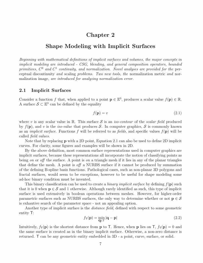
Another type of implicit surface is the distance field, defined with respect to some geometricentity T:

fT(p) = minq∈T

|q − p| (2.2)

Intuitively, fT(p) is the shortest distance from p to T. Hence, when p lies on T, fT(p) = 0 andthe same surface is created as in the binary implicit surface. Otherwise, a non-zero distance isreturned. T can be any geometric entity embedded in 3D - a point, curve, surface, or solid.

7

8

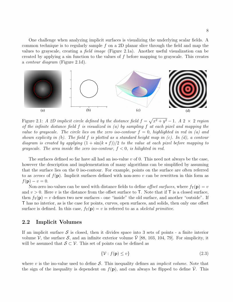
One challenge when analyzing implicit surfaces is visualizing the underlying scalar fields. Acommon technique is to regularly sample f on a 2D planar slice through the field and map thevalues to grayscale, creating a field image (Figure 2.1a). Another useful visualization can becreated by applying a sin function to the values of f before mapping to grayscale. This createsa contour diagram (Figure 2.1d).

Figure 2.1: A 2D implicit circle defined by the distance field f =√

x2 + y2 − 1. A 2 × 2 regionof the infinite distance field f is visualized in (a) by sampling f at each pixel and mapping thevalue to grayscale. The circle lies on the zero iso-contour f = 0, highlighted in red in (a) andshown explicity in (b). The field f is plotted as a standard height map in (c). In (d), a contourdiagram is created by applying (1 + sin(k ∗ f))/2 to the value at each pixel before mapping tograyscale. The area inside the zero iso-contour, f < 0, is hilighted in red.

The surfaces defined so far have all had an iso-value v of 0. This need not always be the case,however the description and implementation of many algorithms can be simplified by assumingthat the surface lies on the 0 iso-contour. For example, points on the surface are often referredto as zeroes of f(p). Implicit surfaces defined with non-zero v can be rewritten in this form asf(p) − v = 0.

Non-zero iso-values can be used with distance fields to define offset surfaces, where fT(p) = vand v > 0. Here v is the distance from the offset surface to T. Note that if T is a closed surface,then fT(p) = v defines two new surfaces - one “inside” the old surface, and another “outside”. IfT has no interior, as is the case for points, curves, open surfaces, and solids, then only one offsetsurface is defined. In this case, fT(p) = v is referred to as a skeletal primitive.

2.2 Implicit Volumes

If an implicit surface S is closed, then it divides space into 3 sets of points - a finite interiorvolume V , the surface S, and an infinite exterior volume V [88, 103, 104, 79]. For simplicity, itwill be assumed that S ⊂ V. This set of points can be defined as

{V : f(p) ≤ v} (2.3)

where v is the iso-value used to define S. This inequality defines an implicit volume. Note thatthe sign of the inequality is dependent on f(p), and can always be flipped to define V . This

9

definition provides a trivial point containment test [104] - the value of f(p) determines where p

is inside or outside the surface.Not all implicit surfaces are necessarily implicit volumes. For example, the distance fields

of the previous section do not define implicit volumes, as Equation 2.3 is true both inside andoutside the surface. Self-intersecting implicit surfaces also cannot define implicit volumes, asthe notion of inside and outside is undefined in the self-intersecting regions. However, if T is aclosed, non-self-intersecting surface, then a signed distance field can be defined where fT(p) < 0if p lies inside T, and fT(p) > 0 outside.

In practice, creating a signed distance field for a non-trivial surface can be very difficult. Thesurface must support both a distance query and a point containment query to define a signeddistance field, and hence an implicit volume. One of the advantages of skeletal primitives, whichalways define implicit volumes, is that they only require the underlying skeletal elements tosupport a distance query [124, 120].

2.3 Solid Modeling

Early 3D modeling systems [88, 85, 86] involved the construction of complex 3D shapes usingsimpler volumes such as spheres, cubes, and cylinders. These simple volumes were composedusing boolean operations such as union (∪), intersection (∩), and subtraction or difference (\).This constructive style of modeling is known as Solid Modeling, or Constructive Solid Geometry(CSG).

Boolean CSG operations are essentially set operations on 3D points. For example, the unionof two 3D volumes is the set of points inside both volumes. In 1973, Ricci [88] introduced avery simple approach to performing set operations between implicit volumes, based on functionalcomposition of the underlying scalar functions. The union of two implicit volumes can be definedas

(f1 ∪ f2)(p) = min (f1(p), f2(p)) (2.4)

This composition operator produces a new scalar field defining a new implicit volume. Intersec-tion and difference can be computed using similar methods.

The power of Ricci’s operators is that they are closed under the space of all possible implicitvolumes, meaning that an application of an operator simply produces another scalar field defininganother implicit volume. This new field can be composed with other fields, again using Ricci’soperators. Equation 2.4 will always produce the exact union of two implicit volumes, regardlessof how complex they are. Compared with the difficulties involved in applying boolean CSGoperations to B-rep surfaces, solid modeling with implicit volumes is incredibly simple. Examplesof Ricci’s CSG operators are shown in Figure 2.2.

2.4 Blending

Solid modeling is not limited to CSG. Another useful class of operation is the construction ofsmooth transitions between two surfaces. These transitions are often known as blends. Onestandard type of blend is the “rolling-ball” blend, where the blend surface is defined by sweeping

10

Figure 2.2: Ricci CSG Operators Union (a), Intersection (b) and Difference (c), applied to circlesin 2D and spheres in 3D.

a sphere along a path such that it just touches both surfaces for all points of the path (essentially“rolling” the sphere around the joint).

Rolling-ball blend surfaces are difficult to compute. However, functional blend operatorssimilar to Ricci’s CSG operators can be defined for implicit volumes. Ricci’s blend operator (]),defined as

(f1 ] f2)(p) =(f1(p)−s + f2(p)−s

) 1

−s (2.5)

produces a new blended volume (Figure 2.3). The parameter s controls the smoothness of theblend (as s → ∞, ] → ∪). This blend operator has the same attributes as the CSG operators,namely that it is independent of surface complexity and that it produces a blended volume whichcan be treated as any other implicit volume.

Figure 2.3: Ricci Blending Operator applied to two circles with blending parameter 6 (a), 12 (b),and 24 (c). A 3D example is shown in (d).

Blinn [24] introduced another type of implicit volume which was based on the concept ofequipotential surfaces in molecular physics. Blinn was trying to visualize molecular structuresusing electron density clouds. The electron density cloud is defined by summing the electrondensity fields of the individual atoms in a molecule. These fields are defined by applying apotential function to a distance field generated from a point p. The specific potential functionwas e−rd2

, where d is the Euclidean distance to p. This field has the value 1 at p and smoothlydecreases to 0 at ∞. The iso-surface is defined by some non-zero v. When the fields generatedby all the points are summed, a smooth blend surface is created.

Blinn’s blobby molecules were essentially implicit skeletal primitives (Section 2.1). HisGaussian potential function can be applied to any skeletal primitive defined by a distance field.These primitives can be blended using the additive blend operator, +:

(f1 + f2)(p) = f1(p) + f2(p) (2.6)

11

Note that this operator is simply a specific case of Ricci’s blend, with s = 1.

2.5 Bounded Fields

While Blinn’s Gaussian skeletal primitives were successful at modeling electron density clouds,they are less useful for interactive modeling. The issue is that the field function e−rd2

has infinitesupport, meaning that its value is non-zero everywhere in space. Since the surface is defined bysummation of all the point primitives, moving any one of them will change the entire surface.For this reason, the primitives are said to have global influence.

Global influence is very un-intuitive for interactive modeling, and particularly for implicitmodeling, where the underlying scalar fields are not visible to the designer. When a primitiveis changed, the expected behavior is that it will only affect the local area. If a primitive hasglobal influence, then changing it locally can affect distant portions of the surface, causing muchconfusion and frustration.

Nishimura [74] and Wyvill et al [124] introduced new polynomial field functions that had finiteor compact support, meaning that the field value is uniformly 0 outside some finite distance fromthe skeletal primitive. Essentially, the non-zero field values are bounded within some geometricregion, and for this reason the skeletal primitives are often said to have bounded fields.

Figure 2.4: Potential functions. (a) Blinn’s Gaussian or “blobby” function, (b) Nishimura’s“metaball” function, (c) Wyvill et al’s “soft objects” function, and (d) the Wyvill function.

The bounded fields used by Nishimura’s Metaballs and Wyvill et al’s Soft Objects are specificcases of a general type of skeletal primitive, defined by composition of a potential function g anda distance field:

f(p) = g ◦ dT(p) (2.7)

This separation is very useful for stating guarantees about scalar fields. If g has compact support,and T is finite, then f will necessarily be bounded. Analysis of some properties of f is alsosimplified - for any convex skeleton, the blending properties of f are completely determined byg. The resulting bounded fields have local influence and hence preserve a sort of “principle ofleast surprise” that greatly improves the usability of constructive implicit modeling.

Most distance field composition operators can be rewritten to work on bounded fields. Forinstance, the Ricci union (Equation 2.4) operator can be converted simply by using max insteadof min (and vice-versa for intersection). The Ricci blend (Equation 2.5) is converted by changing

12

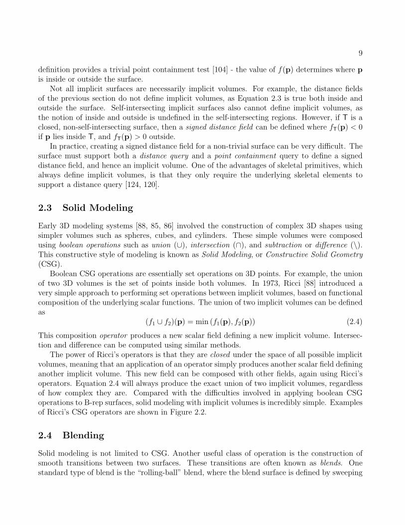
the sign on the blending parameter. CSG difference is more problematic. For bounded fields,one way to define the difference of f1 − f2 is min(f1, 2 v − f2), where v is the iso-value. Thisoperator is problematic because it can produce fields with non-zero values far from the surface.An example is shown in Figure 2.5e, where one skeletal point primitive has been subtracted fromanother. The ring of positive field values in the right side of the image can produce undesirableblending artifacts (See Figure 3.1) and may prevent gradient walks from converging on thesurface. Difference operators based on R-functions (modified to support bounded fields) canreduce the magnitude of these external values, but not eliminate them completely [51].

Clearly, operators acting on bounded fields should produce fields that are also bounded.However, this is a relatively loose requirement - a “bounded field” that stops just short of infinityis still bounded, but cannot really be said to provide local influence. A reasonable constraint(which holds for all the operators described thus far) is that the output bounds be containedwithin the union of the input bounds.

Figure 2.5: Field images of bounded skeletal point primitive (a,b), bounded Bezier curve primitive(c), Ricci blend of point primitives (d), and CSG Difference of point primitives (e).

2.6 Continuity and Manifolds

Many properties of an implicit surface emerge from the mathematical properties of the underlyingscalar field f . One critical property is that of continuity. While continuity comes in many forms,the most basic level of scalar field continuity is C0 continuity. In mathematical terms, a C0-continuous field f is a field where as the distance between two 3D points p and q decreases tozero, so does the difference between their field values f(p) − f(q).

C0 field continuity is one of the basic pre-requisites for a variety of other mathematicalstatements that can be made about f . One desirable property for solid modeling is that any iso-surface of f be a closed simple manifold. In terms of 2D surfaces embedded in three dimensions,a surface is a manifold if some infinitely-small neighbourhood around any point on the surface“looks” like a disc [89]. If a manifold has no boundaries (edges where the surface lies only onone side, such as the edge of a triangle), then it is said to be closed. Closed manifolds whichhave no self-intersections are said to be simple. In 3 dimensions, a closed simple manifold has awell-defined interior and exterior, and hence a well-defined volume. This is nececssary for solidmodeling, as only surfaces with well-defined volumes can be considered solids (Section 2.2). To

13

simplify exposition, a surface will be said to be manifold when it is a closed simple manifold.Note that the iso-surface may include multiple un-connected surfaces, in this case each surfaceis analyzed independently.

Scalar fields can be classified with respect to continuity and manifold properties. Binaryfields are not C0; the field values “jump” between 0 and 1 but do not make smooth transitions.Distance fields are C0, however the manifold properties of the zero iso-contour are determinedentirely by the geometric skeleton. The skeleton may not be closed, may have self intersections,or may not even be a surface. In any of these cases, the zero iso-contour is not manifold1.

Offset surfaces of distance fields are manifold, despite the degenerate interior boundaries thatcan occur at certain iso-values. For example, a degenerate point occurs at the center of the dis-tance field of a sphere when the iso-value is equal to the sphere radius. These interior iso-surfacesare infinitely thin and can be removed using a topological process known as regularization [85]which removes all extraneous lower-dimensional artifacts. Regularization is based on classifyingpoints as either boundary2 or interior, where interior points are those points inside the volume.Hence, regularization cannot repair volumes with self-intersections because the notion of “inside”is no longer mathematically well-defined.

Since offset surfaces of distance fields are manifold, all non-zero iso-contours of skeletal implicitprimitives are manifold. Unlike distance fields, the zero iso-contour is not used in constructivemodeling with bounded skeletal primitives. Hence, for modeling purposes, skeletal primitivesalways produce manifold iso-surfaces. This is a key distinction between skeletal primitives anddistance fields.

Since a constructive modeling system will involve functionally combining implicit surfaces,the mathematical properties of composition operators must also be analyzed. Consider a generalbinary operator g(f1, f2). Iso-surfaces of g(f1, f2) can only be manifold if they are C0, so itis essential that g preserve C0 continuity. As noted by [17], g defines a 2D scalar field whichmaps from E

2 to R. If f1, f2, and g are all C0, then the scalar field produced by g(f1, f2) isguaranteed to be C0. While C0 continuity is a necessary condition for manifold iso-surfaces, itis not sufficient. If f1 = v and f2 = v are manifold, then for most of the standard operators,g(f1, f2) = v is manifold. However, the necessary conditions for g to preserve manifold iso-contours are unknown in computer graphics.

Based on these mathematical properties, certain statements can be made about constructivemodeling with implicit surfaces. One key property is that if the primitives in use are C0 andhave manifold iso-surfaces, and all operators in use are C0 and preserve manifold iso-surfaces,then surfaces created with the system will be C0 and manifold. Using this set of primitives andoperators, it is impossible to create an implicit model that does not define a volume. This is veryuseful for interactive volume modeling, as it means that the designer cannot “break” the systemand produce an invalid model.

1Again, “manifold” is used here as a shorthand here for “closed simple manifold”2The term boundary is used here in a point-set-topology sense [115], boundary points are members of the

closures of both the interior and exterior sets of points. For a valid implicit volume, boundary points are definedby f(p) = v and interior points by f(p) < v.

14

2.7 C1 Continuity and The Gradient

C0 continuity, which ensures that there are no “jumps” in a function, is the most basic form ofcontinuity. Higher-order continuity is defined in terms of derivatives of functions. For example,if the derivative of a one-dimensional scalar function is continuous, then the scalar function hasfirst derivative or C1 continuity.

In the case of a 3D scalar field f , the first derivative is a vector function known as the gradient,written ∇f and defined as:

∇f(p) =

{∂f(p)

∂x,∂f(p)

∂y,∂f(p)

∂z

}(2.8)

If ∇f is defined at all points, and the three one-dimensional partial derivatives are each C0, thenf is C1.

Surfaces have a related but different notion of C1 continuity. Informally, C1 surface continuityrequires that the surface normal vary smoothly over the surface. The surface normal at p is theunit vector perpendicular to the surface. If no unique surface normal can be defined, such as onthe edge of a cube, then the surface is not C1 along the edge. Note that self-intersections arealso not C1, so a closed C1 surface is necessarily manifold 2.6. For points on an implicit surfacef(p) = v, the surface normal can be computed by normalizing the gradient vector ∇f .

Surface continuity has direct implications for computer graphics. Shading on a surface at apoint p is largely controlled by the surface normal. If the surface is not C1, the gradient (andhence the normal) can change direction significantly at the discontinuity. At the C1 discontinuity,a shading artifact will appear when the surface is rendered (Figure 2.6b). Hence, C1 continuityis very desirable for modeling smooth surfaces.

If f is C1, then any iso-surface of f is C1. Unsigned distance fields are never C1. This iseasily shown in 1D, the “distance function” for a point at the origin is simply the absolute valuefunction, which is not C1. Hence, the distance field for any 3D skeleton will not be C1 at theskeleton. Signed distance fields are C1 if the skeleton is convex. If the skeleton is non-convex,then some points in space are equidistant to multiple points on the skeleton. There is no uniquesolution to Equation 2.2, and C1 discontinuities occur in both signed and unsigned fields. Forexample, a C1 discontinuity occurs at the center of the distance field for a sphere.

Skeletal implicit primitives are created by applying a potential function to an unsigned dis-tance field (Equation 2.7). Although the distance field is never C1 at the skeleton, these dis-continuities can be removed by using a suitable potential function [9]. Specifically, if the firstderivative of the 1D potential function is 0 at the origin, then the skeletal primitive becomes C1

on the skeleton. However, C1 discontinuities in the distance field due to non-convex skeletonsare still present in the skeletal primitive field. Note that if the potential function is bounded, itmust also have a zero first derivative when it reaches 0, and must be C1 in the non-zero interval,for any skeletal primitive to be C1.

As with C0 continuity, no discussion is complete without considering the continuity of opera-tors. Again, if f1 and f2 are C1, and g is C1, then g(f1, f2) is necessarily C1. However, analysis ofoperators is complicated by the fact that it is sometimes desirable to create a C1 discontinuity.This case occurs whenever a crease in the surface is desired. For example, a cube is not C1

15

because tangent discontinuities occur at each edge. To create creases using C1 primitives, theoperator must introduce C1 discontinuities, and hence cannot be C1 itself.

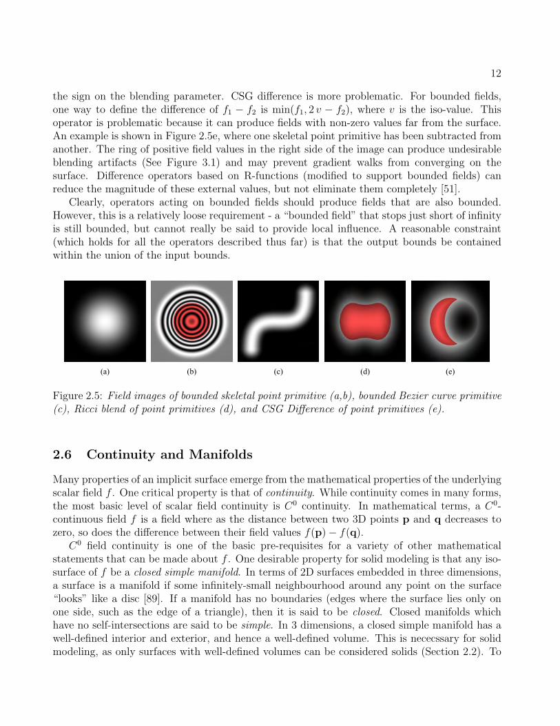
A common type of operator which must create creases are CSG operators, such as union andintersection. However, the manner in which C1 discontinuities are introduced into the field isquite important. For example, the min() union operator (Equation 2.4) creates C1 discontinuitiesat all points where f1(p) = f2(p). When applied to two spheres, the discontinuities produced bythis union operator result in a crease on the surface (Figure 2.6a), which is the desired result.However, the discontinuities extend into the field outside of the surface, which is not visible inthis image. If a blend is then applied to the result of the union, the C1-discontinuous plane inthe field produces a shading discontinuity (Figure 2.6b). To avoid this problem, CSG operatorshave been developed [17] which are C1 at all points except those where f1(p) = f2(p) = v.Hence, creases are only introduced at the v iso-surface, and the shading discontinuity in theblend surface is removed (Figure 2.6c).

Figure 2.6: Point blended to two union of two spheres (a) using C0 Ricci union operator (b) andC1 Barthe union operator (c). The Ricci union has a C1 discontinuity plane which shows upas a crease through the middle of the contour diagram (d). The Barthe contour diagram (e) issmooth except at the desired surface crease.

2.8 Higher Order Continuity and Perceptual Discontinuities

Higher-order continuity is important in many situations. For instance, C2 continuity, also knownas curvature continuity, is a requirement in many engineering applications. The notion of con-tinuity is generalized as Cn continuity, with C∞ being a desirable goal. For instance, Blinn’sGaussian implicits are C∞.

While many skeletal implicit primitives have higher-order continuity, formulating continuity-preserving operators is more difficult. Particularly challenging is the construction of CSG oper-ators, which must introduce C0 creases but also maintain higher-order continuity away from thecreases. For example, Barthe’s operators [17] achieve only C1 continuity.

However, with regards to perceived surface smoothness, continuity is necessary but not suf-ficient. Continuity is a mathematical property of functions. A surface may be C∞ continuous,but appear to have a crease, because of a very high-frequency region in the underlying scalarfield. An example of this situation is shown in Figure 2.7d, where two surfaces are joined with avery sharp blend, and then blended with another. Although there appears to be a crease in thefinal surface, like the C1 discontinuity in Figure 2.6b, the underlying field is in fact C2.

16

Unfortunately these perceptual discontinuities are largely determined by subjective humanjudgement. For example, the apparent crease in Figure 2.7d may disappear when examinedclose-up. This viewer-dependence hinders the construction of mathematical tools for analyzingperceptual discontinuities. Still, there are situations where such high-frequency surface variationsare likely to occur. Perceptual discontinuites will be a factor in the analysis of the implicit surfaceapproximation schemes in Chapters 4 and 5.

Figure 2.7: Additive blending of two point primitives defined by potential functions (1 − d2)n,where n = 2 (a), n = 3 (b), and n = 4 (c). The blend becomes smoother as continuity increases.In (d), a smaller point primitive is blended to two other primitives which have been blended usingEquation 2.5 with a large blending parameter. Although the field is C2, there appears to be adiscontinuity because the underlying field changes very quickly.

2.9 Field Normalization and Surface Convergence

The gradient ∇f of a scalar field encodes two important pieces of information - the maximumrate-of-change of f , and the direction in which this maximum occurs. A desirable property offields useful for implicit modeling is that ∇f always points “towards” the surface. If this is thecase, then it is possible to reach the surface from any point by taking tiny steps in the directionof the gradient3.

Distance fields have two properties related to the gradient which are very useful. First, ina distance field, ∇f always points towards the nearest point on the surface. Second, distancefields are normalized [103, 22]. A normalized field is one in which the gradient has a magnitudeof 1 everywhere in the field (‖∇f(p)‖ = 1). Given these two properties and a point p anywherein space, the nearest point on the surface can be found directly - it is p + f(p)∇f(p). In fact,distance fields are not strictly normalized, because ∇f is undefined at C1 discontinuities (pointson the distance surface, and points equi-distant from the skeleton). In these cases none of thenearest points can be found, since the gradient is undefined. For convenience, these discontinuitieswill be disregarded when discussing normalization.

Normalization is a tenuous property and is very difficult to maintain, especially when combin-ing scalar fields with C1 (or greater) composition operators. Bounded fields by definition cannotbe normalized, since ∇f is 0 outside the bounds. However, even inside the bounds, f can onlybe normalized if the potential function is linear. The smoother potential functions necessary tocreate C1 primitives (Section 2.7) rule out normalization.

3In some fields, the gradient always points away from the surface

17

Even if f is not normalized, it is still possible to use the gradient to converge on the surface.To see how, consider a distance field scaled by 2, f2 = 2fT. In this case, ‖∇f2‖ = 2. Essentially,‖∇f‖ is a measure of the local scaling of the field values, so the nearest point to p on the surfaceis

p +f2(p)∇f2(p)

‖∇f2(p)‖(2.9)

Unfortunately, on bounded fields such as those in Figure 2.5, evaluating this equation will notproduce a point on the iso-surface. One consequence of normalization is that all higher-orderderivatives are 0. In non-normalized fields where the higher-order derivatives are non-zero (suchas in smooth bounded fields), Equation 2.9 only approximates the correct distance. However,repeated application of Equation 2.9 will eventually produce a point on the surface under somerelatively weak conditions 4. This iteration is known as surface convergence. Note that if thesurface iso-value v is non-zero, then the convergence iteration is instead:

p +(f(p) − v)∇f(p)

‖∇f(p)‖(2.10)

These convergence iterations assume that ∇f(p) is non-zero. One drawback of bounded fieldsis that the gradient is zero in most of space. Hence, Equation 2.10 will only converge on thesurface if the start point has a non-zero field value. In fields with infinite support, convergenceoccurs from any point in space.

Surface convergence is a critical tool for visualizing implicit surfaces, and in this domain itis desirable that surface convergence occur as quickly as possible. Higher normalization errorin non-linear fields generally leads to a larger number of iterations of Equation 2.10 necessaryto reach a given error tolerance, as each step is more likely to under-shoot or over-shoot thesurface. Normalization also has other benefits [22]. For example, in a normalized field, anoffset surface created by modifying the iso-value is equivalent to a distance-based offset surface.Also, normalized fields have a consistent “blending radius” which makes the results of blendingoperations more consistent and predictable. Tools for evaluating normalization are described inthe next section.

2.9.1 Analyzing Field Normalization Error

Strict normalization is generally not attainable for the scalar fields used in implicit modeling.Even if the fields of primitives are normalized, few operators preserve normalization, particularlyblending operators. However, since normalization is a key property for predictable implicit mod-eling, it is useful to be able to compare the normalization error in different fields. Normalizationerror at a point p is defined as |1 − ‖∇f(p)‖|, and a normalization metric over a field f 5 canthen be defined as:

normf = maxp

(|1 − ‖∇f(p)‖|) (2.11)

4The convergence step is essentially a Newton iteration, which is known to be relatively stabe [84] but is onlyguaranteed to find the nearest local minimum. Hence, it is necessary that the field be monotonic along the pathto the surface.

5In bounded fields, only the normalization error at points where f 6= 0 should be considered.

18

In a normalized field, normf = 0. However, unles f is described by a simple equation, analyti-cally computing normf is not possible. The only alternative is to discretely approximate normf

by sampling over some domain. Besides the maximum, various other statistical measures can beapplied to the samples to further analyze the normalization error. If the sampling is regular, avisual analysis tool called a normalization image can be constructed in the same way as field im-ages (Section 2.1). Normalization images permit a more detailed evaluation of the normalizationerror in a particular scalar field. Some examples are shown in Figure 2.8.

Figure 2.8: Normalization images for (a) bounded skeletal point primitive, (b) CSG differenceof bounded point primitives, and (c) Ricci blend of point primitives. The error scale runs from0 (black) to ≥ 1 (white). The normalization image for the blended circles from Figure 2.2b isshown in (d). Since they are distance fields, the result is normalized everywhere except in theblending region.

Normalization error is also visible in contour images. If f is normalized, the spacing betweencontours is perfectly regular. As the normalization error increases, contour spacing changes, andcan be irregular over the field. The normalization error in a bounded point primitive is clearlyvisible when comparing the contour image to that of a circle’s distance field, as in Figure 2.5b.

2.10 The Scaling Problem

A fundamental issue with skeletal primitive modeling is the scaling problem. Consider a singlepoint primitive, generated by the composition of some potential function with the distance fieldof a single point. The question is, how can the size of this point primitive be altered, or scaled?

If the iso-surface is defined as f(p) = v, then one option is to change v. However, consider amore complex case - two points are blended together. How can one be scaled? If v is modified,both will be scaled. The only solution to scaling primitives is to modify f .

At this point, it is useful to introduce a specific potential function. The following potentialfunction, gw, will be used for all skeletal primitives that follow:

gw(d) =

(1 −

(d2

r2

))3

(2.12)

where r is the “radius” of the field and the input distance d is clamped to the range [0, r] [123].Generally, an iso-value of 0.5 is used with this function. The function is C6 continuous and does

19

have zero-tangents at either end. A plot of gw is shown in Figure 2.4d, and an additive blend oftwo point primitives with r = 1 is shown in Figure 2.10d.

Figure 2.9: The scaling problem. To create a blend between two point primitives of different radius(a), the potential function must be scaled. The resulting iso-contours of the smaller primitive aremore closely spaced (b) due to higher normalization error (c). The normalization error increasesas the primitive becomes smaller.

By modifying r, the desired scaling result in Figure 2.9 is achieved, however the region of thefield containing the scaled primitive has significantly more normalization error than the regionof the un-scaled field. The difference in normalization error has many undesirable effects. Animmediately visible problem is that it results in variable blending behavior when primitives withdifferent scaling factors are blended (Figure 2.10). Another issue is that the convergence iteration(Equation 2.10) will require more steps to reach the same level of accuracy. This is the scalingproblem.

Figure 2.10: The sequence of images in (a)-(c) show how the scaling problem creates blends whichare less smooth than when the primitives all have the same scale (d).

There are several possible approaches to mitigating the scaling problem. The first is tomodify the potential function. Consider the plots in Figure 2.11a, showing gw with radius 1and 0.5. At values > 0.5, the scaled function can be improved by “flattening” the 1D function,such that the value at gw(0) is less than 1 (Figure 2.11b). However, The scaled function mustdecrease from 0.5 to 0. To improve this region, the function must extend further along the xaxis (Figure 2.11c). However, this “long tail” causes the field to extend further out in space fromthe iso-surface, increasing the support region of the primitive and breaking the principle of localsupport (Section 2.5). Blending with the resulting field can be very un-intuitive.

20

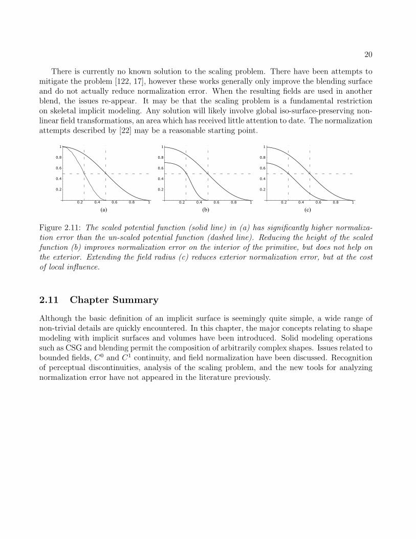
There is currently no known solution to the scaling problem. There have been attempts tomitigate the problem [122, 17], however these works generally only improve the blending surfaceand do not actually reduce normalization error. When the resulting fields are used in anotherblend, the issues re-appear. It may be that the scaling problem is a fundamental restrictionon skeletal implicit modeling. Any solution will likely involve global iso-surface-preserving non-linear field transformations, an area which has received little attention to date. The normalizationattempts described by [22] may be a reasonable starting point.

Figure 2.11: The scaled potential function (solid line) in (a) has significantly higher normaliza-tion error than the un-scaled potential function (dashed line). Reducing the height of the scaledfunction (b) improves normalization error on the interior of the primitive, but does not help onthe exterior. Extending the field radius (c) reduces exterior normalization error, but at the costof local influence.

2.11 Chapter Summary

Although the basic definition of an implicit surface is seemingly quite simple, a wide range ofnon-trivial details are quickly encountered. In this chapter, the major concepts relating to shapemodeling with implicit surfaces and volumes have been introduced. Solid modeling operationssuch as CSG and blending permit the composition of arbitrarily complex shapes. Issues related tobounded fields, C0 and C1 continuity, and field normalization have been discussed. Recognitionof perceptual discontinuities, analysis of the scaling problem, and the new tools for analyzingnormalization error have not appeared in the literature previously.

Chapter 3

A Taxonomy of Implicit Surfaces

A series of functional properties, introduced in the previous chapter, are chosen for use in a clas-sification of different implicit modeling systems. Major hierarchical implicit modeling frameworksand other recent implicit surface modeling schemes are classified based on these properties. Thistaxonomy is used to select a method for use in an interactive modeling system. The hierarchicalBlobTree implicit modeling framework is chosen.

3.1 Introduction

As noted in the previous chapter, any scalar function in E3 inevitably defines some implicit sur-

face. However, depending on the task, certain functions are “more useful” than others. Unfortu-nately there is little consensus on which types of implicit surfaces are appropriate for interactivemodeling. In the following sections, an attempt is made to classify a variety of existing implicitsurface techniques, based on their mathematical properties. The goal of this taxonomy is to sup-port comparisons between different methods, with an eye towards selecting a implicit modelingframework that will best support interactive modeling.

As with any taxonomy, the properties which are chosen to differentiate different implicit sur-face schemes are somewhat at the whim of those creating the taxonomy. Likewise, the groupingof different implicit surface techniques into the considered categories is somewhat arbitrary, butnecessary to make the task tractable. Even more problematic is the fluidity of implicit surfaces.Attributes of a binary nature, such as whether or not a function is bounded (Section 2.5), arequite rare. Many other important properties, such as normalization error considerations, do notpermit such easy categorization. In these cases the statements about different techniques mustbe qualified with often imprecise terms.

In short, the following classification is proposed only as an initial attempt, and was designedwith interactive modeling in mind. For the task of selecting a technique for interactive modelingwith implicit surfaces, it has served its purpose. These biases must be considered when applyingthis taxonomy to other domains.

Another caveat is that the properties mentioned below are largely based on mathematicalaspects, rather than algorithmic issues. This limitation of scope has been enforced due to thecomplexity of classifying algorithmic properties. For example, some implicit modeling techniqueshave special properties which can be taken advantage of to provide faster visualization [7]. De-pending on the application, these fast techniques may not produce the desired accuracy or visualproperties. Which specific visualization problems should be selected as most important? Fur-thermore, any discussion of visualization speed is intimately tied to implementation quality andcomputing hardware. In most cases, source code is not available, and any attempts to normalizecomputation times between 10-year-old computers and state-of-the-art networked clusters arelikely to be erroneous. In short, detailed analysis of these issues for a single implicit repre-

21

22

sentation scheme is non-trivial, and attempts to generalize across the range of implicit surfacetechniques considered in this chapter would undoubtedly fail. Hence, this taxonomy is limitedto mathematical issues of shape representation, as outlined in Section 1.3.

3.2 Classification Properties

Continuity The notions of C0 and C1 continuity, as well as the generalization to Ck continuity,were discussed in Sections 2.6 and 2.7. Field continuity is a critical property for determiningwhen an implicit surface technique is appropriate for a given application. For constructiveimplicit modeling frameworks, continuity of Boolean CSG (Section 2.3) and blending operators(Section 2.4) will also be considered.

Field Support As discussed in Section 2.5, some fields have finite support, meaning that theirnon-zero values are contained within some finite bounding region. This property is often desirablefor computational reasons, however in interactive modeling a more critical implication is that oflocal influence. Of course, an unbounded field can always be explicitly bounded, so statementsmade about this property will generally refer to the support of the field as it is commonly usedin the literature.

Analytic Surfaces Many types of implicit surfaces are defined based on a given set of 3Dpoint samples {pi, fi}, such that they either interpolate or approximate the values fi at pi.These techniques generally cannot represent simple analytic surfaces such as a sphere or cylinder.Techniques which support these types of basic surfaces will be said to be analytic.

Creases The modified definition of C1 continuity given in Section 2.7 permits C1 discontinuitieson the surface to represent creases, which are critical in 3D modeling. This is a binary propertyfor most implicit surface repesentations, however in some cases there is limited support for certaintypes of creases (such as the explicit creases created in MPU methods).

Guaranteed Volumes Most types of implicit surfaces are also capable of defining implicitvolumes (Section 2.2). However, only some methods are guaranteed to generate surfaces withoutself-intersections, and hence well-defined volumes. Further, for constructive implicit modelingframeworks, this property must be preserved regardless of the operators and primitives involved(Section 2.6).

Expected Volumes For some types of bounded implicit surfaces defined based on point sam-ples, internal iso-contours can occur which result in a well-defined but undesirable volume. Theseinternal iso-contours are highly problematic in solid modeling contexts. Since the expected vol-ume is somewhat subjective, for point-sampled surfaces the general requirement will be that alliso-contours lie on or very near to the initial samples. In constructive implicit modeling the oper-ators must be considered; the resulting volume will be expected if all iso-contours are connectedto one of the iso-contours of the input fields.

23

Normalization Error Normalization error was introduced in Section 2.9. In general, fieldswith low normalization error lead to well-behaved and efficient algorithms, particularly with re-spect to surface-convergence steps. Low normalization error also results in blending behaviorthat is more consistent, allowing designers to more easily manipulate blend surfaces. Normaliza-tion error is highly variable and currently cannot be distilled down into a simple categorization- each case must be analyzed independently.

3.3 Constructive Modeling Frameworks

Implicit surface modeling techniques generally take one of two paths. The first is to constructcomplex shapes by composing of simpler shapes (primitives) [88, 124, 120, 4, 106, 18, 58, 11]. Thesecond is to construct complex shapes directly, generating a single scalar field from some given setof surface or volume samples [92, 35, 113, 34, 72, 114, 56, 73, 75, 87, 105]. Systems taking the firstapproach will be referred to as constructive modeling framework, while the second will be termedglobal field approaches. This distinction is somewhat artificial, as any global field techniquecan be used as a primitive in constructive systems [18]. However, there is a clear conceptualdistinction, which is supported by the literature - works on global implicit representation rarelyanalyze the resulting fields for compatibility with constructive frameworks. For example, manyefficient techniques for interpolating 3D point sets produce additional iso-contours [72, 75, 87].While not a significant problem for their intended application (surface reconstruction from rangescans), these extra iso-surfaces have serious implications for solid modeling.

3.3.1 Distance Fields, R-Functions, and F-Reps

Procedural modeling with distance fields is perhaps the oldest application of implicit volumemodeling [88]. However, the introduction of R-functions [90] for shape modeling was a majoradvance [104]. R-functions provide a robust theoretical framework for boolean composition ofreal functions [103, 79], permitting the construction of Cn CSG operators. These CSG operatorscan be used to create blending operators simply by adding a fixed offset to the result [79].Although these blending functions are no longer technically R-functions [103], they have most ofthe desirable properties and can be mixed freely with R-functions to create complex hierarchicalmodels. These R-function-based blending and CSG operators will be referred to as R-operators.

While any partition of the real line does in theory have a set of associated R-operators, thepartition used most frequently in computer graphics is such that the zero iso-contour is takenas the surface, positive values inside, and negative values outside [103, 104, 79]. This impliesthat all fields have infinite support, and all operators necessarily have global influence. The termF-Rep is often used to refer to this class of implicit solid models [4].

As noted in Section 2.6, any surface can be represented as the zero iso-contour of a distancefield. While this does mean that both analytic surfaces and creases are inherently supported, itis also possible to describe non-manifold surfaces with F-Reps. Hence, no volumetric guaranteescan be made. R-operators exist for both signed and unsigned distance fields. In the unsignedcase, volumes are not defined, and furthermore the composition of manifold surfaces can produce

24

non-manifold results. With signed fields, if all initial surfaces are manifold, volume guaranteescan be made.

In general, composition with R-operators produces fields with very poor normalization, evenif the initial fields are normalized [17, 22, 51]. Recent work has focused on improving normaliza-tion [17, 22], however the results are limited (see Section 5.2).

R-operators do not inherently require distance fields. Any distance-like fields (fields with thedesired iso-contour at v = 0) can be composed. Hence, the F-Rep framework can be applied toa wide variety of implicit surfaces.

3.3.2 BlobTree Modeling

Skeletal primitives (Section 2.5) are defined as offset surfaces in a potential field, and have anonzero iso-value. In addition, skeletal primitives with finite skeletons are bounded. The R-operators used in F-Rep systems cannot be applied to these fields, and hence an alternate setof blending operators has been developed. While Shapiro [103] states that a set of R-functionsmust exist for such fields, they have not been extensively studied in the literature1. Some recentattempts to adapt CSG R-operators have been made [16, 51], however these operators simplyconvert the bounded field to an unbounded F-Rep, apply standard R-operators, and explicitlybound the result.

The BlobTree [120] hierarchical modeling framework encapsulates techniques for construc-tive modeling with skeletal primitives. In general, skeletal primitives have variable continuitydepending on the potential function, although low-degree polynomials (k ≤ 6) are most com-mon. Regardless, Boolean CSG operators which produce higher than C1 fields are currentlyunknown [19]. Analytic surfaces can be represented, creases can be represented exactly, andstrong volume guarantees can be made. However, existing CSG difference operators for boundedfields [88, 120, 16, 19, 51] leave non-zero values far from the surface, which can result in unex-pected additional iso-surfaces after additive blending is applied (Figure 3.1).

Figure 3.1: A CSG Difference operation on two point primitives (a) leaves a ring of non-zerovalues far from the surface. When combined with additive blending, These values can causeunexpected behavior (b,c) and additional unwanted iso-contours (d).

Significant scale differences beween skeletal primitives will result in high normalization error

1Ricci’s min and max CSG operators [88] do appear to be R-functions, however they are rarely identifed assuch. Also, CSG operators based on R-functions are described by Wvill et al [120], however it is unclear whetheror not they are actually R-functions.

25

(Section 2.10). Repeated additive blending also increases normalization error, particularly forvolumes that overlap significantly. Attempts to mitigate this problem using global field trans-formations have met with limited success [51].

The BlobTree framework does not inherently require that all primitives be skeletal primitives.The only condition is that values inside the surface be larger than the nonzero iso-value, andthat the field drops off to 0 at some distance outside the surface. The sweep templates generatedin Chapter 5 are one example of non-skeletal bounded fields.

3.3.3 Convolution Surfaces

Convolution surfaces, first introduced by Bloomenthal and Shoemake [28], are produced by con-volving a geometric skeleton S with a kernel function h. Hence, the value at any position inspace is defined by an integral over the skeleton:

f(p) =

∫

S

g(r) h(p − r) dr (3.1)

Any compactly-supported function can be used as h, see [107] for a detailed analysis of differentkernels.

Like skeletal primitives, convolution surfaces have bounded fields. Since they are compatiblewith the BlobTree modeling framework, they are in some sense a special case of skeletal prim-itives. However, composition of convolution surfaces is usually defined by composition of theunderlying geometric skeletons, rather than functional composition. The reason for this is toavoid the bulges that tend to occur when composing multiple skeletal primitives with additiveblending. The surface resulting from convolution of the combined skeleton does not have bulges,and the field is continuous even if the combined skeleton is non-convex. Volumes are preserved,and normalization error is entirely dependent on the convolution kernel. However, because theyare always offset a fixed distance from a geometric skeleton, convolution surfaces cannot representcreases or non-smooth analytic surfaces.

3.4 Uniformly-Sampled Discrete Volume Datasets

Given a set of samples fi of some f(p) distributed at uniform intervals, a scalar field f canbe constructed which approximates f [35]. The sets of samples are often referred to as volumedatasets. The properties of the constructed scalar field hinge on the technique used to convertthe fi to f . Generally, a reconstruction filter is applied to the samples in some neighbourhoodof p to produce a continuous field using interpolation. Although Ck spline-based reconstructionfilters can be used, C0 to C2 are most common [69, 71]. Field support is arbitrary - the sample set

is assumed to be finite, so the value of f(p) outside of the sample set is application-defined. Aswith any sample-based scheme, analytic surfaces can only be approximated. Similarly, arbitrarycreases cannot be represented. Volume and normalization properties are completely dependent onthe sample set, no general statements can be made in these cases. Implicit surfaces created usingvolume datasets may be compatible with either the F-Rep or BlobTree modeling frameworks,and can be used to define Convolution Surfaces [101].

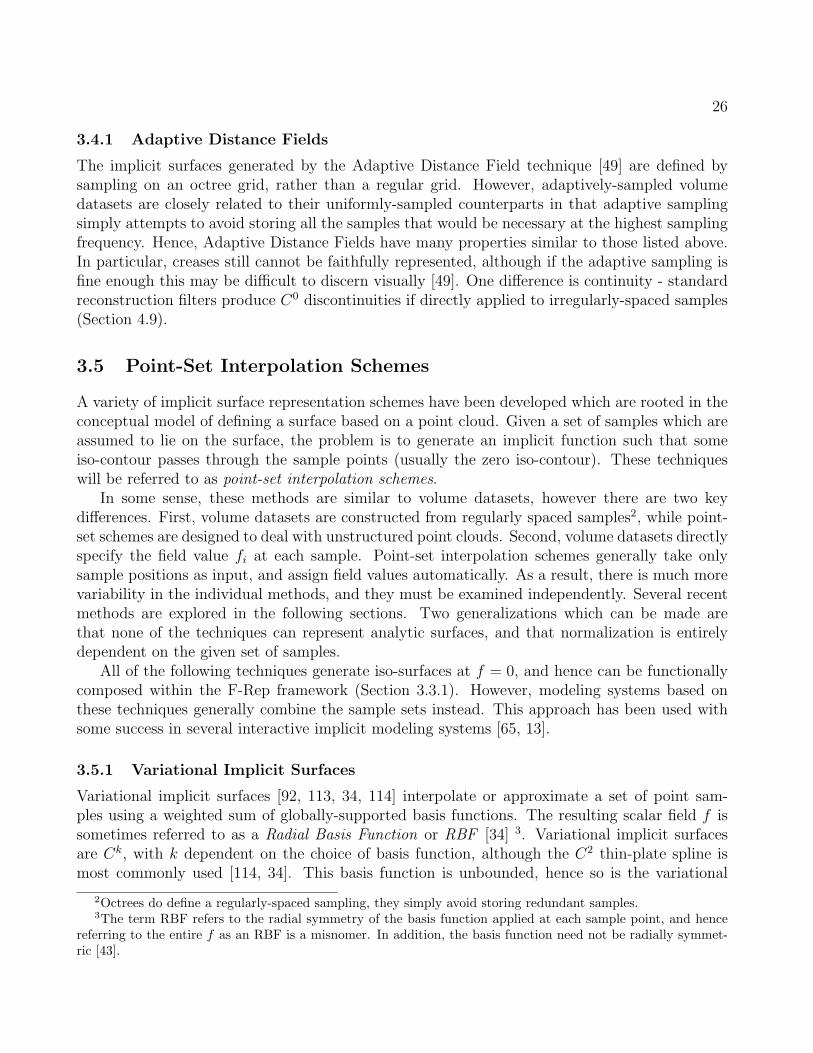
26

3.4.1 Adaptive Distance Fields

The implicit surfaces generated by the Adaptive Distance Field technique [49] are defined bysampling on an octree grid, rather than a regular grid. However, adaptively-sampled volumedatasets are closely related to their uniformly-sampled counterparts in that adaptive samplingsimply attempts to avoid storing all the samples that would be necessary at the highest samplingfrequency. Hence, Adaptive Distance Fields have many properties similar to those listed above.In particular, creases still cannot be faithfully represented, although if the adaptive sampling isfine enough this may be difficult to discern visually [49]. One difference is continuity - standardreconstruction filters produce C0 discontinuities if directly applied to irregularly-spaced samples(Section 4.9).

3.5 Point-Set Interpolation Schemes

A variety of implicit surface representation schemes have been developed which are rooted in theconceptual model of defining a surface based on a point cloud. Given a set of samples which areassumed to lie on the surface, the problem is to generate an implicit function such that someiso-contour passes through the sample points (usually the zero iso-contour). These techniqueswill be referred to as point-set interpolation schemes.

In some sense, these methods are similar to volume datasets, however there are two keydifferences. First, volume datasets are constructed from regularly spaced samples2, while point-set schemes are designed to deal with unstructured point clouds. Second, volume datasets directlyspecify the field value fi at each sample. Point-set interpolation schemes generally take onlysample positions as input, and assign field values automatically. As a result, there is much morevariability in the individual methods, and they must be examined independently. Several recentmethods are explored in the following sections. Two generalizations which can be made arethat none of the techniques can represent analytic surfaces, and that normalization is entirelydependent on the given set of samples.

All of the following techniques generate iso-surfaces at f = 0, and hence can be functionallycomposed within the F-Rep framework (Section 3.3.1). However, modeling systems based onthese techniques generally combine the sample sets instead. This approach has been used withsome success in several interactive implicit modeling systems [65, 13].

3.5.1 Variational Implicit Surfaces

Variational implicit surfaces [92, 113, 34, 114] interpolate or approximate a set of point sam-ples using a weighted sum of globally-supported basis functions. The resulting scalar field f issometimes referred to as a Radial Basis Function or RBF [34] 3. Variational implicit surfacesare Ck, with k dependent on the choice of basis function, although the C2 thin-plate spline ismost commonly used [114, 34]. This basis function is unbounded, hence so is the variational

2Octrees do define a regularly-spaced sampling, they simply avoid storing redundant samples.3The term RBF refers to the radial symmetry of the basis function applied at each sample point, and hence

referring to the entire f as an RBF is a misnomer. In addition, the basis function need not be radially symmet-ric [43].

27

implicit surface. Since the field is globably C2, creases cannot be defined. Anisotropic basisfunctions [43] can be used to produce fields which change more rapidly and may appear to havecreases, however the surface is still smooth when inspected at the appropriate scale. The smoothfield implies that self-intersections do not occur, and hence volumes are always well-defined. Thethin-plate spline guarantees that global curvature is minimized [44], which intuitively seems toimply that internal zero iso-contours will not occur. However, no formal proof could be located4.

Variational inteprolation has many properties which are desirable for 3D modeling, howevercontrolling the resulting surfaces is very difficult. In Chapter 5, variational interpolation will beused to generate free-form skeletal primitives.

3.5.2 Compactly-Supported Variational Implicit Surfaces

Variational implicit surfaces based on compactly-supported radial basis functions (CS-RBFs)were proposed as a technique to reduce the computational cost of variational interpolation tech-niques [72]. Each CS-RBF only influences a local region, so computing f(p) only requires eval-uation of basis functions with some small neighbourhood of p. As with the globally-supportedcounterpart, the resulting field is Ck, creases are not supported, and self-intersections cannotoccur. The local support of each basis function results in a bounded global field, however thisalso guarantees that additional iso-contours will be present, as noted by various authors [75, 87].

3.5.3 Multi-level Partition of Unity Implicits

Multi-Level Partition of Unity (MPU) Implicit Surfaces [75] are defined by a set of point con-straints with normals. Similar to compactly-supported variational implicit surfaces, the basictheory behind MPU implicits is to subdivide space into regions and construct a local implicitapproximation of the surface in each region. To evaluate f(p), overlapping basis functions areblended using partition-of-unity weights generated using Ck functions. However, to optimizeconstruction an adaptive octree-based spatial subdivision technique is used. Several basis func-tions have been applied, [75] uses C1 quadrics while [87] uses local Ck radial basis functionsThese basis functions produce unbounded fields, hence the global field is unbounded.

Certain types of creases can be represented on a per-cell basis by fitting multiple quadricsurfaces and combing them using functional CSG operators. However, cells with creases mustbe detected based on the deviation of the point set normals. This procedure is far from robust,limiting [75] to edges (two surfaces) and corners (three surfaces)). However, [87] notes thatthe local creases are not preserved by the partition-of-unity blending functions. The quadricrepresentation guarantees that volumes are defined, and the octree-based decomposition reducesthe possibility of unwanted internal iso-surfaces, but there is no guarantee that they are voidedcompletely.

4The author admits only limited familiarity with the related mathematical literature, so such a proof mayindeed exist.

28

3.5.4 Implicit Moving Least-Squares

The Implicit moving least-squares (IMLS) technique [105] is closely related to MPU methods.The major improvement is the addition of value constraints over entire triangles, allowing entiretriangle meshes to be exactly interpolated. Interpolation can also be relaxed, creating smootherapproximations to the original mesh. Normal constraints are also improved, to reduce ringingartifacts. As with MPU implicits, various Ck basis and weighting functions can be used. Sinceadjacent triangles can be interpolated exactly, IMLS can represent creases, but only if exactinterpolation is used - approximating implicit surfaces are always smooth. If the initial mesh isself-intersecting, the IMLS surface will reproduce these self-intersections, and possibly introduceothers. Since the basis functions have global support, unwanted internal iso-contours are unlikelyto occur, however it is unclear if this is guaranteed.

3.6 Classification Summary

In the previous sections, a variety of implicit surface modeling techniques have been analyzed withrespect to the properties described in Section 3.2. The results of this analysis are summarized inFigure 3.2. The columns in the table correspond to the properties listed in Section 3.2, and therows to the various implicit modeling schemes. In an attempt to be as conservative as possible,any properties about which there is some debate are marked as having “limited support”. Inthese cases, the analyses in the previous sections should be consulted.

The Continuity column lists the maximum continuity that can be achieved, including blend-ing and CSG operations for the constructive frameworks. The Bounded, Analytic Surfaces,Creases, and Guaranteed Volumes columns are essentially either-or properties, although sometechniques have limited support. The Expected Volumes column indicates what little is knownabout this property. Likewise, the Normalization Error column provides only a relative rankingamong the constructive techniques - very little can be said about discrete volumes and point setinterpolation.

3.7 Selecting a Modeling Framework

Ideally, an interactive implicit modeling system would support any implicit surface modelingtechnique. However, certain incompatibilities, such as bounded vs unbounded fields, prevent thecomposition of different types of fields. To construct an internally consistent modeling system, aspecific modeling technique must be selected. The purpose of the classification developed in thischapter was to assist with such a choice.

Some desirable properties are already known. Guaranteed validity, ie the impossibility ofcreating self-intersecting surfaces which do not define a volume, is clearly beneficial. The abilityto represent analytic surfaces is useful in engineering contexts. The local influence provided bybounded fields leads to more intuitive results during interaction with the model. Already, thepossible choices have been narrowed down to two modeling frameworks - BlobTree modeling andConvolution Surfaces.

29

Figure 3.2: Implicit Surface Classification Quick Reference Chart

30

Convolution surfaces do have some compelling benefits. In particular, they have the mostcontrollable normalization error of all the techniques described above. Unfortunately the skeletal-composition approach used in convolution surface modeling can only represent smooth surfaces.While this is clearly a promising direction for future work, one must currently step outside of theconvolution framework into a more general modeling system, such as the BlobTree, to performbasic operations such as boolean CSG.

Hence, the BlobTree remains as the only implicit modeling framework which supports thedesired properties. The main drawback of the BlobTree is that only C1 CSG operators arecurrently known. However, this is an area of active research, and smoother methods may bedeveloped in the future. Similarly, the problematic non-monotonic field generated by CSG dif-ference operations is likely avoidable. Normalization error does seem to be an inherent problem(Section 2.10), however unlike in the R-operator case, the problem is localized by the bounds ofthe relevant fields. Additional control over normalization error may be possible using boundedblending operations [51].

3.8 Chapter Summary

Classifying mathematical functions is a difficult task, perhaps best left to mathematicians. Unfor-tunately, mathematicians seem to have largely neglected issues relating specifically to interactivecomputer graphics systems. Hence, in this section a set of functional properties have been iso-lated and used to classify a set of recent implicit surface modeling techniques. Both hierarchicalmodeling frameworks and schemes based on discrete samples have been classified. The result is ataxonomy of schemes which has been used to select a specific system, the BlobTree hierarchicalmodeling framework, for use in an interactive system.

A final note must be made to emphasize that this classification is only a preliminary attempt.Like the animation-specific comparative study presented in [33], it is biased towards its intendedapplication - 3D modeling. The taxonomy presented here is not intended to be the final word onthe subject, but rather a tool for recognizing the current limitations of implicit volume modeling.

Chapter 4

Hierarchical Spatial Caching

Issues relating to interactive visualization of BlobTrees are introduced. An analysis of existingcaching schemes leads to a novel new approach called Hierarchical Spatial Caching. Conceptualand practical implementation issues are discussed. Profiling results show an order-of-magnitudeimprovement in visualization times. Adaptive Distance Fields are analyzed for use in this cachingscheme, and found to be unsuitable.

Some material in this chapter is taken from the publication “Interactive Implicit Modeling withHierarchical Spatial Caching” by Schmidt, Wyvill, and Galin [97]. The material appearing hereis due to Schmidt. The Medusa model was provided by Galin.

4.1 The Interactive Visualization Problem

One of the critical constraints on interative tools for hierarchical constructive implicit modeling isthe cost of visualizing the model. Although volume visualization techniques are becoming morecommon, traditional 3D modeling interfaces are based on the notion of manipulating surfaces.Unfortunately, the surface S defined by f(p) = v is in some sense unknown. Unlike a parametricsurface patch, there is no function to evaluate which outputs points on the surface. Withoutan explicit surface function, visualization algorithms must resort to spatial searches to find thesurface. These methods generally produce a discrete sampling of the surface, this sampling canthen be rendered interactively.

A variety of spatial search algorithms for sampling the implicit surface have been developed.Most approaches produce triangle meshes [124, 109, 53, 5, 64, 93, 57] or point clouds [117, 56, 70,110]. Regardless of the sampling technique, the fundamental operation in all of these algorithmsis finding points on (or near) the surface by evaluating f(p). Most algorithms rely on somegeometric approach to find points “near” the surface, and then refine these guesses, convergingon the surface using repeated evaluations of f(p).

When visualizing complex implicit surfaces, these convergence steps (Section 2.9) consumethe majority of the computational effort. As an example, a profiling test was performed on arelatively simple model (100 blended randomly-positioned point primitives) using a standardpolygonization algorithm [26]. The f(p) function was programmed using hand-optimized andtuned SIMD assembly code, to maximize performance. In this case, at moderate triangle reso-lutions the evaluation of f(p) consumed 95% of the CPU time. At production-quality triangleresolutions the cost of f(p) increased to 99%. Similar results have been observed with othervisualization algorithms.

Clearly, the cost of visualizing an implicit surface with spatial search algorithms is directlydependent on the cost of evaluating f(p). Recent visualization algorithms [70] often reporttimes of multiple seconds or minutes to sample complex implicit surfaces. Unfortunately, a key

31

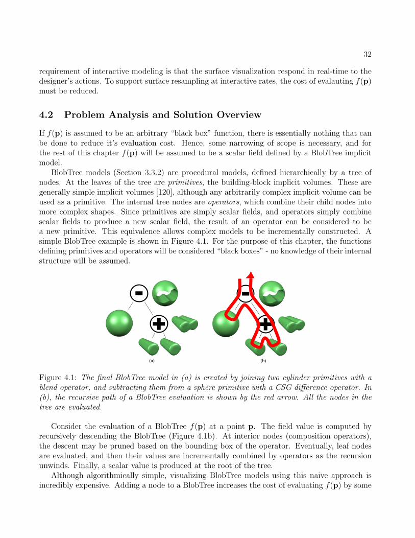
32

requirement of interactive modeling is that the surface visualization respond in real-time to thedesigner’s actions. To support surface resampling at interactive rates, the cost of evalauting f(p)must be reduced.

4.2 Problem Analysis and Solution Overview

If f(p) is assumed to be an arbitrary “black box” function, there is essentially nothing that canbe done to reduce it’s evaluation cost. Hence, some narrowing of scope is necessary, and forthe rest of this chapter f(p) will be assumed to be a scalar field defined by a BlobTree implicitmodel.

BlobTree models (Section 3.3.2) are procedural models, defined hierarchically by a tree ofnodes. At the leaves of the tree are primitives, the building-block implicit volumes. These aregenerally simple implicit volumes [120], although any arbitrarily complex implicit volume can beused as a primitive. The internal tree nodes are operators, which combine their child nodes intomore complex shapes. Since primitives are simply scalar fields, and operators simply combinescalar fields to produce a new scalar field, the result of an operator can be considered to bea new primitive. This equivalence allows complex models to be incrementally constructed. Asimple BlobTree example is shown in Figure 4.1. For the purpose of this chapter, the functionsdefining primitives and operators will be considered “black boxes” - no knowledge of their internalstructure will be assumed.

Figure 4.1: The final BlobTree model in (a) is created by joining two cylinder primitives with ablend operator, and subtracting them from a sphere primitive with a CSG difference operator. In(b), the recursive path of a BlobTree evaluation is shown by the red arrow. All the nodes in thetree are evaluated.

Consider the evaluation of a BlobTree f(p) at a point p. The field value is computed byrecursively descending the BlobTree (Figure 4.1b). At interior nodes (composition operators),the descent may be pruned based on the bounding box of the operator. Eventually, leaf nodesare evaluated, and then their values are incrementally combined by operators as the recursionunwinds. Finally, a scalar value is produced at the root of the tree.

Although algorithmically simple, visualizing BlobTree models using this naive approach isincredibly expensive. Adding a node to a BlobTree increases the cost of evaluating f(p) by some

33

factor m, where m is the cost of evaluating the new node. Assuming that the surface is sampledwith k points, and n convergence steps are taken to refine each sample position, then addingadding a new primitive increases the cost of sampling the surface by m ·n · k operations. If thesefactors are assumed to be constant, then the visualization time doubles as the number of nodesin the tree doubles.

While linear growth is generally considered quite good from a theoretical standpoint, in prac-tice the resulting explosion in computational cost prohibits usable interactive BlobTree modelingsystems. Simple models can be manipulated in real-time, however as the timings in Section 4.8.2clearly show, existing methods are several orders of magnitude too slow to support high-qualityinteractive visualization of even moderately complex models.

Since primitives and operators are assumed to be “black boxes”, there are few opportunitiesfor optimization in the basic algorithm. Discarding the “black-box” formalism is undesirable.The power of BlobTree modeling is largely derived from it’s generality, of which the “black-box”notion is a critical component. Hence, the only avenue for reducing evaluation cost is to evaluatefewer tree nodes.

In the following sections, a method will be developed for replacing sub-trees of a BlobTreemodel with dynamically-computed scalar field approximations. These approximate scalar fieldscan be evaluated in constant time, reducing the cost of evaluating the approximated subtreefrom O(N) to O(1). To avoid unnecessary pre-computation overhead, the approximate scalarfields are generated using dynamic lazy evaluation. This Hierarchical Spatial Caching techniqueis both a caching and an approximation scheme. In a variety of tests, use of hierarchical spatialcaching has been found to produce an order of magnitude reduction in visualization time overexisting techniques.

4.3 Previous Caching and Approximation Schemes

A common approach to reduce the cost of visualizing an implicit surface is to employ cachingschemes. Caching techniques generally try to exploit coherence in the global state of the Blob-Tree. Caching can happen at many levels, from very coarse caching at the level of inter-frametemporal coherence, to very fine caching of node-specific variables during during a BlobTreetraversal.

Local update schemes [62, 117, 42, 53, 5, 14] cache surface samples, exploiting temporalcoherence to reduce the number of evaluations of f(p). When the BlobTree is modified, localsupport ensures that the changes in f(p) are bounded within some region B. The surface outsideB is guaranteed to be unmodified, and hence the samples outside B need not be recomputed.Local update schemes do improve interactivity, and can be used with most other caching schemes.However, they do not fundamentally reduce the cost of evaluating f(p), so large or complexupdate regions are still problematic.

BlobTree traversals can also be cached, to some extent. One approach is to generate a cachetree [48, 51]. A cache tree mirrors the BlobTree, containing a cache node for each tree node.Temporary variables and field values computed during the last tree traversal are stored in eachcache node. The cached values are only valid if the tree is traversed multiple times at a point p.

34

Cache trees provide a speed-up mainly in situations where the field value and gradient are bothcomputed at p. If p changes between each evaluation, cache trees actually make evaluation off(p) more expensive. A similar approach involves pre-computing values that will be constantalong a 3D ray [15].

Another take on caching traversals is to subdivide space into voxel “bins” and prune theBlobTree at each bin [48]. The BlobTree is traversed for each voxel, and a new tree is constructedwhich only contains nodes that intersect the current bin. These pruned trees are used instead ofthe original tree to evaluate f(p). This scheme is based on the observation that for a complexBlobTree containing nodes with many children, a large number of redundant bounding box testsmay be performed. The pruning step is too expensive to perform interactively, and must berepeated whenever the tree is modified. Similar speed-ups could likely be achieved with less pre-computation by dynamically generating bounding box hierarchies at nodes with many children.However, like cache trees, while performance is definitely improved, the gains are not sufficientto provide interactivity.

The caching schemes mentioned so far are essentially optimization techniques. Visualizationtime is reduced by avoiding redundant computation, but the cost of visualizing a BlobTree isnot fundamentally reduced. To achieve this, approximation schemes have been developed whichrepresent the implicit surface using a BlobTree which has fewer nodes, or nodes that are lessexpensive to evaluate. For example, [29] suggests replacing expensive spline primitives with aset of blended points primitives. This concept has been generalized as level-of-detail or LODimplicits [15]. Curve and surface primitives based on subdivision skeletons [12, 58] provide asimple framework for LOD primitives. However, LOD primitives are problematic for interactivemodeling because lower levels of detail do not accurately reflect the final model. Even if thesurface of the LOD primitive is relatively accurate at lower detail levels, the underlying fieldmay be different, producing a different surface after blending. LOD primitives also only reducecomputational cost at the leaves of the tree, the techniques do not generalize to approximatingthe result of composition nodes.

Caching and approximation is combined in spatial caching schemes. A basic spatial cachecan be created by sampling f(p) on a uniform grid. The field value at any p can then beapproximated by applying a reconstruction filter, such as tri-linear interpolation, to a set ofsamples near p. This type of spatial cache can support level-of-detail by reducing or increasingthe number of samples stored in the cache. General spatial caches simply approximate the scalarfield f(p), instead of attempting to explicitly approximate the implicit surface, and hence canbe applied to both primitives and composition nodes.

Barthe [18] describes a general constructive modeling system based on quadratic interpolationof uniformly-sampled grids (which are essentially spatial caches). The system allows a designerto interactively combine two shapes, creating a new sampled grid. The new grid can againbe combined with another, resulting in a binary tree of composition operations. To conservememory, the tree of grids is not stored, hence the user can only manipulate the root node (orappend a new node). Frisken [49] describes a similar system but replaces the uniform gridswith adaptively-sampled distance fields (ADFs) to improve the representation of small details.Again, tree editing is only supported at the root node - the the notion of procedural modelingis essentially discarded. Without the hiearchical framework, benefits of the BlobTree such as

35

animation and non-linear editing are lost.Akleman [7] describes a related type of spatial caching for ray-tracing certain classes of

implicit surfaces known as ray-quadric surfaces. These primitives, when evaluated along a ray,reduce to quadratic functions which can be easily solved. The function coefficients can be cached,permitting quick ray-surface intersection tests. Ray quadrics can also be functionally composed,using a somewhat-cumbersome interface based on manipulation of 3D prisms [7]. However,individual ray-quadrics are limited to “star-shapes” and the caching techniques do not generalizefor use in general constructive modeling systems.

The use of spatial caches in these works demonstrates the computational benefits of approx-imating analytic scalar fields with discrete sampling. However, none of these systems providedfully interactive BlobTree-style modeling. Akelman’s [7] caching system does not generalize toblack-box hierarchical modeling. The memory and processing limitations inherent in Barthe’s [18]approach prevent non-linear editing of the model tree, and hence many of the benefits of hiearchi-cal modeling are lost. Kizamu [49] suffers from a similar limitation. In some sense, because theunderlying analytic functions are discarded, it is debatable that the use of spatial approximationin [18] and [49] should even be called caching. Regardless, while the desired level of interactivitywas not achieved, the results are promising and suggest that further investigation is warranted.

4.4 Hierarchical Spatial Caching

To address the shortcomings of previous applications of spatial approximation to hierarchicalimplicit modeling, the Hierarchical Spatial Caching method was developed. The underlyingidea in Hierarchical Spatial Caching is is to dynamically insert spatial caches into the BlobTree.These spatial caches are re-cast as cache nodes which can be placed above any other internalnode in the BlobTree. The samples of f stored in the caches are dynamically computed asthey are needed. The hierarchical caches are also dynamically invalidated (and recomputed) asthe designer modifies the BlobTree. The main components of Hierarchical Spatial Caching aredescribed in the following paragraphs.

In previous works, spatial caches have been used at the primitives and at the root of thehierarchical model tree. Primitive caches do not reduce the cost of evaluating complex trees.In the BlobTree, where primitives are relatively inexpensive to evaluate [120], primitive cachesprovide little benefit. Global caches do reduce the cost of evaluating f . However, considerthat during interactive manipulation, some region of f is being modified and hence the cachein that region must be invalidated and recomputed. Similar to local update schemes, if themodified region is large or expensive to evaluate, the global cache fails to preserve interactivity.In particular, global caching provides marginal benefit if a local update scheme is used for surfacevisualization.

In contrast to primitive and global caches, the approach taken in hierarchical spatial caching isto insert spatial caches inside the BlobTree. As noted above, there is marginal benefit to cachingindividual primitives or the root node, so caches are only placed above internal compositionoperator nodes. The spatial cache is then formalized in the BlobTree framework as a cache node.A caching node C is a unary operator with a single subtree T . Each caching node stores a set

36

of exact potential field values determined by evaluating its subtree T . When evaluating thepotential field of T at a point p inside the bounding box of T , an approximation fC(p) to theexact potential field value fT (p) is reconstructed from the cached potential values. The subtreeT is not traversed, reducing the cost of evaluating it from O(N) to O(1) (Figure 4.2).

Figure 4.2: In (a), two cylinder primitives are blended, and then subtracted from a sphere. In (b),a cache node is inserted above the blend node, reducing the cost of evaluating the blend sub-tree.

Previous applications of spatial approximation to constructive implicit modeling have entirelyreplaced the analytic functions with discretely-sampled grids [18, 49]. In this situation, all gridsamples must be stored and updated at all times. However, in the case of cache nodes, theunderlying analytic BlobTree functions are not discarded. Hence, cache samples can be computedon-demand, and there is no reason to store fully evaluated grids. When a cache node is to beevaluated at a point p, the cache data structure is inspected to determine if the samples requiredto reconstruct fT (p) are available. If some are not, they are first computed, and then fC(p) isevaluated. In short, cache nodes are filled using lazy evaluation (Figure 4.3).

Lazy evaluation is a significant benefit, as full evaluation of high-resolution grids is computa-tionally intensive. In addition, if surface-tracking visualization algorithms are used, only cachesamples near the surface are necessary. In this case most of the samples in a fully evaluated gridwill never be used - particularly if they will be invalidated in the next frame as the user drags aprimitive across the screen.

Since Hierarchical Spatial Caching involves replacing analytic scalar functions with discretesamplings, it is an approximation scheme. However, because cache nodes are dynamically ini-tialized based on evaluations of f(p), and subtree traversals are dynamically truncated, cachenodes can also be considered traversal caches. The novelty of Hierarchical Spatial Caching isthe combination of spatial approximation with traversal caching. Individually, these techniqueshave limited ability to reduce the cost of interactive visualization for a complex BlobTree. Whencombined they can produce an order-of-magnitude reduction in visualization time.

37

Figure 4.3: Lazy evaluation process. In (a), the field values necessary to reconstruct the valueat the incoming query point (in blue) are unavailable. The child field must be evaluated 4 times,once for each cache value (b). In (c), two cache values are missing and must be evaluated in thechild field (d). Finally, in (e) all cache values are available. The incoming value query can bedirectly approximated in O(1) time, no O(N) evaluations of the child field are necessary.

4.5 Hierarchical Spatial Caching Implementation Issues

A number of design decisions must be made when implementing hierarchical spatial caching. Thechoice of sampling scheme is paramount to the performance and accuracy of any spatial approx-imation scheme, however several other implementation details hold regardless of the particularsampling scheme.

The first issue relates to dynamic cache invalidation. During tree traversals in a standardBlobTree implementation, child nodes are evaluated by their parents. Child nodes never initiateevents - there is no upward communication. However, to implement dynamic cache invalidation,there must be some mechanism to tell a parent node when it’s child has been modified. Eachnode on the path from the modified child to the root node must be notified, so that any cachenodes on the path have a chance to discard now-invalid cache values.

There are essentially two option for implementing this parent notification. One option isto use an external notification scheme - an “oracle”, which knows about all the nodes in themodel tree and can explicitly notify them. This scheme preserves the top-down organizationof the BlobTree - children do not need to know their parents. Also, the oracle can accumulateinvalidation events and then only notify each node once, which can be more efficient if multiplechildren change simultaneously. The second option is to use a parent-notification scheme, whereinvalidation events are passed up the model tree from child to parent. This scheme preservesthe desirable BlobTree properties of encapsulation and local knowledge, at the cost of possiblerepeated notifications. There is no clear winner between these options. The oracle introducessignificant implementation complexity, however the upward-notification approach may be lessefficient.

The actual process of invalidating a cache node is somewhat dependent on the particular

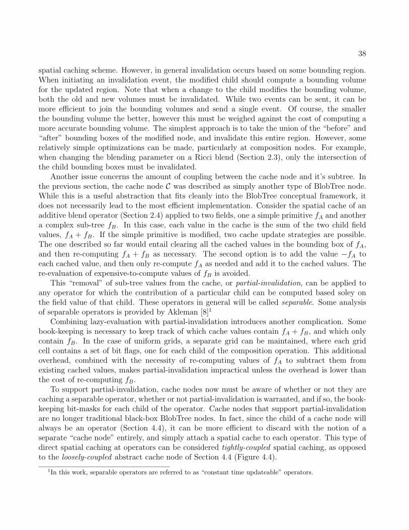
38

spatial caching scheme. However, in general invalidation occurs based on some bounding region.When initiating an invalidation event, the modified child should compute a bounding volumefor the updated region. Note that when a change to the child modifies the bounding volume,both the old and new volumes must be invalidated. While two events can be sent, it can bemore efficient to join the bounding volumes and send a single event. Of course, the smallerthe bounding volume the better, however this must be weighed against the cost of computing amore accurate bounding volume. The simplest approach is to take the union of the “before” and“after” bounding boxes of the modified node, and invalidate this entire region. However, somerelatively simple optimizations can be made, particularly at composition nodes. For example,when changing the blending parameter on a Ricci blend (Section 2.3), only the intersection ofthe child bounding boxes must be invalidated.

Another issue concerns the amount of coupling between the cache node and it’s subtree. Inthe previous section, the cache node C was described as simply another type of BlobTree node.While this is a useful abstraction that fits cleanly into the BlobTree conceptual framework, itdoes not necessarily lead to the most efficient implementation. Consider the spatial cache of anadditive blend operator (Section 2.4) applied to two fields, one a simple primitive fA and anothera complex sub-tree fB. In this case, each value in the cache is the sum of the two child fieldvalues, fA + fB. If the simple primitive is modified, two cache update strategies are possible.The one described so far would entail clearing all the cached values in the bounding box of fA,and then re-computing fA + fB as necessary. The second option is to add the value −fA toeach cached value, and then only re-compute fA as needed and add it to the cached values. There-evaluation of expensive-to-compute values of fB is avoided.

This “removal” of sub-tree values from the cache, or partial-invalidation, can be applied toany operator for which the contribution of a particular child can be computed based soley onthe field value of that child. These operators in general will be called separable. Some analysisof separable operators is provided by Akleman [8]1

Combining lazy-evaluation with partial-invalidation introduces another complication. Somebook-keeping is necessary to keep track of which cache values contain fA + fB, and which onlycontain fB. In the case of uniform grids, a separate grid can be maintained, where each gridcell contains a set of bit flags, one for each child of the composition operation. This additionaloverhead, combined with the necessity of re-computing values of fA to subtract them fromexisting cached values, makes partial-invalidation impractical unless the overhead is lower thanthe cost of re-computing fB.

To support partial-invalidation, cache nodes now must be aware of whether or not they arecaching a separable operator, whether or not partial-invalidation is warranted, and if so, the book-keeping bit-masks for each child of the operator. Cache nodes that support partial-invalidationare no longer traditional black-box BlobTree nodes. In fact, since the child of a cache node willalways be an operator (Section 4.4), it can be more efficient to discard with the notion of aseparate “cache node” entirely, and simply attach a spatial cache to each operator. This type ofdirect spatial caching at operators can be considered tightly-coupled spatial caching, as opposedto the loosely-coupled abstract cache node of Section 4.4 (Figure 4.4).

1In this work, separable operators are referred to as “constant time updateable” operators.

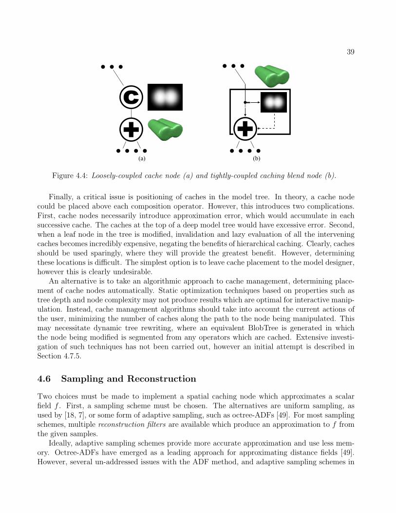
39

Figure 4.4: Loosely-coupled cache node (a) and tightly-coupled caching blend node (b).

Finally, a critical issue is positioning of caches in the model tree. In theory, a cache nodecould be placed above each composition operator. However, this introduces two complications.First, cache nodes necessarily introduce approximation error, which would accumulate in eachsuccessive cache. The caches at the top of a deep model tree would have excessive error. Second,when a leaf node in the tree is modified, invalidation and lazy evaluation of all the interveningcaches becomes incredibly expensive, negating the benefits of hierarchical caching. Clearly, cachesshould be used sparingly, where they will provide the greatest benefit. However, determiningthese locations is difficult. The simplest option is to leave cache placement to the model designer,however this is clearly undesirable.

An alternative is to take an algorithmic approach to cache management, determining place-ment of cache nodes automatically. Static optimization techniques based on properties such astree depth and node complexity may not produce results which are optimal for interactive manip-ulation. Instead, cache management algorithms should take into account the current actions ofthe user, minimizing the number of caches along the path to the node being manipulated. Thismay necessitate dynamic tree rewriting, where an equivalent BlobTree is generated in whichthe node being modified is segmented from any operators which are cached. Extensive investi-gation of such techniques has not been carried out, however an initial attempt is described inSection 4.7.5.

4.6 Sampling and Reconstruction

Two choices must be made to implement a spatial caching node which approximates a scalarfield f . First, a sampling scheme must be chosen. The alternatives are uniform sampling, asused by [18, 7], or some form of adaptive sampling, such as octree-ADFs [49]. For most samplingschemes, multiple reconstruction filters are available which produce an approximation to f fromthe given samples.

Ideally, adaptive sampling schemes provide more accurate approximation and use less mem-ory. Octree-ADFs have emerged as a leading approach for approximating distance fields [49].However, several un-addressed issues with the ADF method, and adaptive sampling schemes in

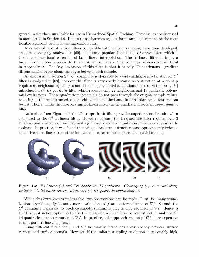
40

general, make them unsuitable for use in Hierarchical Spatial Caching. These issues are discussedin more detail in Section 4.9. Due to these shortcomings, uniform sampling seems to be the mostfeasible approach to implementing cache nodes.

A variety of reconstruction filters compatible with uniform sampling have been developed,and are thoroughly analyzed in [69]. The most popular filter is the tri-linear filter, which isthe three-dimensional extension of basic linear interpolation. The tri-linear filter is simply alinear interpolation between the 8 nearest sample values. The technique is described in detailin Appendix A. The key limitation of this filter is that it is only C0 continuous - gradientdiscontinuities occur along the edges between each sample.

As discussed in Section 2.7, C1 continuity is desirable to avoid shading artifacts. A cubic C2

filter is analyzed in [69], however this filter is very costly because reconstruction at a point p

requires 64 neighbouring samples and 21 cubic polynomial evaluations. To reduce this cost, [71]introduced a C1 tri-quadratic filter which requires only 27 neighbours and 13 quadratic polyno-mial evaluations. These quadratic polynomials do not pass through the original sample values,resulting in the reconstructed scalar field being smoothed out. In particular, small features canbe lost. Hence, unlike the interpolating tri-linear filter, the tri-quadratic filter is an approximatingfilter.

As is clear from Figure 4.5, the C1 tri-quadratic filter provides superior visual results whencompared to the C0 tri-linear filter. However, because the tri-quadratic filter requires over 3times as many neighbour samples and significantly more computation, it is more expensive toevaluate. In practice, it was found that tri-quadratic reconstruction was approximately twice asexpensive as tri-linear reconstruction, when integrated into hierarchical spatial caching.

Figure 4.5: Tri-Linear (a) and Tri-Quadratic (b) gradients. Close-up of (c) un-cached sharpfeatures, (d) tri-linear interpolation, and (e) tri-quadratic approximation.

While this extra cost is undesirable, two observations can be made. First, for many visual-ization algorithms, significantly more evaluations of f are performed than of ∇f . Second, theC1 continuity necessary to produce smooth shading is only is only required in ∇f . Hence, athird reconstruction option is to use the cheaper tri-linear filter to reconstruct f , and the C1

tri-quadratic filter to reconstruct ∇f . In practice, this approach was only 10% more expensivethan a pure tri-linear approach.

Using different filters for f and ∇f necessarily introduces a discrepancy between surfacevertices and surface normals. However, if the uniform sampling resolution is reasonably high,

41

and the polygonization resolution is on the order of the grid resolution, then these differencesare not visually apparent. A more serious problem may occur for surface-convergence algorithmswhich assume that ∇f points towards the surface. This may not be true with mixed filters, soa pure tri-quadratic approach would be necessary.

One final issue with both the tri-linear and tri-quadratic filters is that it is not possibleto reconstruct sharp edges. As shown in Figure 4.5, the tri-linear filter smooths out creasesexcept when the crease lies on the edge between two samples. The tri-quadratic filter smoothsout all creases. In fact, all the uniform-sampling reconstruction filters analyzed by [69] fail toreproduce sharp edges. Similar problems are encountered with adaptive sampling. A claim hasbeen made that ADFs can reconstruct sharp edges [49], however this is technically not accurate.Due to very high sampling resolution, ADF surfaces appear to have creases when viewed from adistance. However, when viewed from closer distances the same problems as shown in Figure 4.5dwill appear, since ADFs use tri-linear reconstruction.

4.7 A Sample Spatial Caching Implementation

To analyze the performance benefits of hierarchical spatial caching, a sample C++ implemen-tation was created. As discussed in Section 4.6, uniform grids appear to currently be the mosteffective approach to dynamic spatial caching, and are used in the test system. By default, tri-linear reconstruction is used for field values and tri-quadratic reconstruction for field gradients,although these options can be toggled interactively.

In terms of the design options described in Section 4.5, the test implementation utilizestightly-coupled caches attached to composition operator nodes. Parent-notification based on axis-aligned bounding boxes is used for cache invalidation, rather than an external oracle. Althoughfar from optimal, the union of “before” and “after” bounding boxes is used for invalidation inall cases.

An automatic cache placement algorithm is applied (described below), however caching at anoperator node can be directly controlled by the designer. Automatic cache placement is not con-trolled directly by the operator nodes, rather a central cache manager object determines whetherthe cache at an operator should be enabled. This manager can also perform some rudimentaryautomatic model tree optimizations, such as removing redundant composition operators.

A variety of specific optimizations and enhancements have been implemented to improvethe results of hierarchical spatial caching. These improvements are discussed in the followingsections.

4.7.1 Dynamic Grid Resolution

Reconstruction accuracy is entirely dependent on the uniform grid resolution. To reduce under-and over-sampling, the test implementation defines the initial cache resolution based on the axis-aligned bounding box of the subtree T and a user-defined grid resolution r. Let s denote thelongest side of the bounding box of T . The size of each grid cell is then defined as

c = s/r

42

If the bounding box of T changes (due to some interactive operation), a new cell size c′ iscomputed. If the ratio c′/c is greater than 2 or less than 0.5, the current cache is destroyed, andthe cache cell size set to c′. This prevents cache resolution both from getting too low, whichwould result in a coarse approximation of the surface, as well as from getting too high and wastingmemory. Based on empirical observations, an default value of r = 128 provided reasonable cacheaccuracy without excessive update overhead.

No attempt is made to transfer the existing cache values to the new cache. In the case of under-sampling this would clearly be undesirable. It may be beneficial in over-sampling situations,however these seem to be fairly rare in practice, so this optimization was not implemented.Instead, the lazy evaluation scheme automatically re-populates the cache as required.

4.7.2 Cache Coordinate System

Some of the most common operations in interactive modeling are the basic affine transformations- translation, rotation, and scaling. In a naive implementation, these transformations would beapplied to the child of a caching node, causing an expensive cache invalidation. A more efficientapproach is to apply the transformation to the cache itself. In the test implementation, each cachehas a local coordinate system. Affine transformations applied to the operator node are applied tothe associated cache coordinate system as well. This avoids any unnecessary invalidation whentransforming the operator node.

Note that avoiding affine-transformation invalidation is more complicated when using loosely-coupled cache nodes (Section 4.5). In that case, transformation nodes are required, and transfor-mations applied to the child of a cache should always be pushed above the cache node. Ensuringthis behavior again requires a global view of the BlobTree.

4.7.3 Blocked Memory Allocation

High-resolution uniform 3D grids can require significant amounts of memory. A fully-evaluated1283 cache of single-precision floating point values requires 8MB of memory. Current hardwarelimitations prevent storing a significant number of fixed caches at this resolution. In addition, thevolume represented by a single cache can expand, making a fixed grid data structure undesirablebecause it must then be re-allocated.

To reduce memory usage and avoid expensive re-allocation, uniform 3D grids in the testimplementation were allocated using a blocked memory scheme. The uniform grid is dividedinto k × k × k blocks of voxels, where k is the block resolution. A voxel block is allocated onlywhen one of the voxels it contains is needed to compute a field value. The blocks are quicklyidentified using a 30-bit hash, with 10 bits per integer grid axis coordinate [118]2. This approachsaves memory because continuation methods for polygonizing implicit surfaces [26] are designedto follow the surface, hence the required voxels will also be near the surface. Blocks further fromthe surface may remain completely untouched, and hence unallocated. As k decreases, fewer andfewer blocks need be allocated, further reducing memory usage.

2This method limits the total grid size to (1024 · k)3 voxels with 32-bit integers.

43

However, k also affects the cost of sampling and cache invalidation. Sampling is more ex-pensive because the required neighbours of a particular cell may lie in other blocks, which thenneed to be looked up with a relatively expensive hash-table access (compared to simply adding aconstant to the current index). The smaller the block size, the more likely this is to occur. Also,invalidation becomes more expensive because the invalidated cells must be processed block-by-block. As k decreases it becomes increasingly expensive to find and invalidate all the affectedblocks. On the test system, good results were found with a grid resolution of k = 8. Reduc-ing k to 4 cut average memory usage by approximately 20%, but increased update times byapproximately 25%.

Block size also influences low-level hardware efficiency. Current workstation processors con-tain several levels of hardware memory cache to reduce memory access latency. The traditionalstatic allocation of a large 3D uniform grid causes frequent cache misses, particularly when ac-cessing adjacent voxels along the z axis. This blocked allocation scheme potentially increasesprocessor cache coherency if the block size fits in a cache line, although this effect is difficult toisolate.

Memory requirements can be reduced even further by using an encoding scheme, at theexpense of some reconstruction accuracy. The range of potential field values that can occur inour system is small. Memory usage can be reduced 50− 75% percent by encoding floating pointvalues as one or two-byte integers. This technique is slightly more computationally expensiveand decreases accuracy, so it is not used in the test implementation.

4.7.4 Last-Access Caching

As noted in the previous section, looking up the required neighbour values to evaluate a recon-struction filter at a particular grid cell can be a significant cost. The blocked memory schemeonly increases this cost. To offset this expense, a last-access cache is employed. During recon-struction filter evaluation, the cached neighbour values are saved. If the next filter evaluationoccurs in the same cell, the saved values can be used directly, avoiding the relatively expensiveneighbour cell lookups.

While it may seem unlikely that the last-access cache would provide much benefit, duringconvergence iterations 2.9 the same cell is often accessed multiple times. The speed-up providedby last-access caching has not been analyzed, however it introduces negligible overhead so thereis really no reason not to use it.

4.7.5 Dynamic Cache Placement

As noted previously, the efficacy of hierarchical spatial caching is dependent on the positioning ofcaches in the model tree. The automatic cache-placement algorithm used in the test implemen-tation is relatively simple. Placement decisions are based on two assumptions - that primitivesare quick to evaluate, and that most interactive operations take place near the root of the tree.

First, caches are only allocated to operator nodes that have at least two children. Mostoperators have no effect on a single child, and the child will either be an operator with a cache,or a primitive. Based on the fast-primitive assumption, caches are also not allocated if all thechildren of an operator are primitives. Second, caches are only allocated to nodes within n levels

44

from the root node, where n is a small integer (n = 3 in the test implementation). Caches thatfall below this threshold as the model tree changes are discarded.

These rudimentary placement rules prove to be quite effective in practice. In particular, forthe prototype system described here, a quick response is seen for interactive operations performednear the root of the tree. Operations closer to the tree leaves are slower, however in many casesthis can be mitigated by re-organizing the model tree to favor breadth over depth. For example,the sketch-based interface 6 simply appends nodes to the top of the tree. If a body is drawnfirst, and then an arm, the body is a child of the arm and is slow to manipulate. If the treeis manually re-organized, overall interactivity is greatly increased. This leads to the conclusionthat interfaces which assist in the creation of well-organized model trees may be more effectiveat increasing caching efficiency than smarter cache-placement algorihtms.

4.8 Results and Analysis

Hierarchical Spatial Caching has been evaluated in the context of the ShapeShop modelingsystem (Chapter 6). To analyze performance, polygonization times with and without cachingnodes have been compared. The polygonizer in use is an an optimized version of the implicitsurface polygonizer described in [26] with the optional cubical decomposition enabled. Whencomputing a mesh vertex on a cube edge, 10 bisections were performed to locate the implicitsurface.

The software was compiled using the Microsoft Visual Studio 2003 C++ compiller in Releasemode with default optimization flags. All timings reported below were performed on a laptopwith an Intel 1.6Ghz Mobile Pentium 4 processor and 512MB of RAM.

Detailed profiling has been carried out using the complex hierarchical Medusa model shownin Figure 4.6. The model is composed of 9490 point skeletal elements segmented into 7 majorcomponents. Each major component is modeled as a blend of point skeletal elements distributedalong a set of splines. All the points along each individual spline are grouped together into asingle optimized blend node to avoid excessive tree traversal costs. The point counts of the 7components are shown in Figure 4.6.

A caching node with a resolution of 1283 voxels3 was placed above each major componentin the model tree. Potential field reconstruction accuracy was evaluated by comparing recon-structed and exact field values at triangle mesh vertices. Using this method, the mean tri-linearreconstruction error for the Medusa model with 1283 voxel caches is estimated to be approxi-mately 3%, computed by comparing the real and approximate field values at mesh vertices. Theerror is concentrated in high-frequency regions, particularly the head. While a global measure ofreconstruction accuracy has not been devised, it is suspected that the global error will be simi-lar to the near-surface error because the cache spacing is uniform. Also, note that the modelingtechnique of blending many points along spline curves used to create the medusa model producesvery high normalization error (Section 2.9), resulting in higher approximation error.

While the results discussed in this section focus on the Medusa model, the reductions in

31283 was chosen because powers-of-two produce the most efficient memory alignment, and it was the lowestvalue which produced a smooth approximation of all the Medusa components, see Figure 4.9.

45

Figure 4.6: Medusa model composed of 9490 point primitives (left) grouped into 7 major compo-nents - lower body, upper body, neck, chest, left hand, hair, and head. Note that the right handis part of the upper body component, while the left hand is separated.

computation time have been found to apply to found to apply to hierarchical implicit modelingin general. Comparable measurements have been observed with a wide variety of other simple andcomplex models. The Medusa model is focused on here because it is the most computationallyexpensive model that was available and has a wide range of feature scales.

4.8.1 Static Polygonization Time

Static polygonization times for the Medusa model with and without caching nodes are comparedin Table 4.1. All caches were cleared before each polygonization, and all reported times are anaverage of 5 tests. In all cases the cached polygonization contained less than 1% more trianglesthat the non-cached polygonization.

Cubes Cache No Cache Ratio

323 5.77 4.90 0.8×

643 10.34 14.36 1.4×

1283 17.40 51.97 3×

2563 29.23 199.37 6.5×

5123 49.83 809.66 16×

Table 4.1: Comparison of cached and non-cached polygonization times (in seconds) for Medusamodel at different polygonization resolutions.

Polygonization time without caching increases by approximately a factor of 4 when resolutiondoubles. Polygonization time with caching is initially slower than without because 8 voxels arerequired to compute a single tri-linear interpolation. Subsequently, polygonization time reducesas the cache is populated. The ratio between cached times at consective resolutions decreases

46

because more cached voxels are re-used. At 5123 polygonizer resolution, approximately 33% ofall cache voxels have been evaluated.

Since caches are cleared before each polygonization, it may seem un-intuitive that such alarge gain would be made. However, as previously noted, the convergence iterations used torefine surface vertex positions (Section 2.9) frequently involve multiple evaluations in a singlecache cell. With caching, these convergence steps require only a few tri-linear interpolations,instead of evaluation of thousands of point primitives.

While static polygonization time does not provide an indicative measure of interactive perfor-mance, fast static polygonization can still be useful in interactive modeling contexts. A standardinteractive visualization technique is iterative refinement, where the designer interacts with alow-resolution visualization which is automatically refined during idle moments [29]. The exam-ple in Figure 4.7 shows that Hierarchical Spatial Caching is capable of providing significantlyfaster iterative refinement for implicit modeling.

Figure 4.7: Since the cache is already partially evaluated, iterative refinement of the low-resolutionmesh on the left (computed at a polygonizer resolution of 643) takes approximately 6 seconds.The high-resolution refined mesh on the right (computed at 2563 cube resolution) takes over 200seconds to generate without hierachical spatial caching.

4.8.2 Interactive Polygonization Time

While caching nodes can significantly reduce static polygonization time, the critical benefit be-comes apparent during interactive manipulation of BlobTree model components. Update timesmeasured during a a basic interaction test on the Medusa model are compared in Figure 4.8.The test involved simulated translation of the Medusa head component. The head was moved25 steps towards the tail, then 25 steps back to the original position, as shown in the figure.Along this path the head intersects all other components of the model. An initial polygonizationwas computed before running each test, hence the cache begins partially evaluated. Polygonizerresolution was fixed at 603 cubes, based on the initial model bounding box. Note that this is sig-nificantly lower than the resolution shown in Figure 4.8, see Figure 4.7 for a mesh of comparableresolution.

Polygonization time is relatively constant for the non-cached cases, which is expected. Withcaching nodes the polygonization time rapidly drops over the first few frames. Many of thecaching node voxels for the head component are being evaluated over these frames. During the

47

Figure 4.8: Update time with various cache and model configurations for the head-translation testshown on the right. The animation frame is plotted on the X axis - frame 25 corresponds to theright image, frames 1 and 50 to the left. Hierarchical Spatial Caching is an order of magnitudefaster in equivalent tests.

rest of the downward path small numbers of potential field values are cached for other componentsas the head intersects them. This results in a relatively stable polygonization time. At frame 25the upward path begins. The average stable polygonization time drops at this point because allthe necessary field values have been cached on the downward pass.

Tests were performed with and without the hair component. The first few frames are com-puted more quickly without the hair component, however the stable polygonization time isessentially identical in both cases. This comparison shows that after the caches are populated,polygonization time is insensitive to the underlying model complexity and depends primarilyon surface complexity. Finally, polygonizer resolution is doubled to 1203 cubes. The cachedpolygonization converges to a stable time of approximately 1.25 seconds per frame. Non-cachedtimings were over 50 seconds per frame.

4.8.3 Local Update Polygonization

A common technique for improving interactive visualization time in implicit modeling systems isto only re-polygonize the model in areas that have been updated. Several tests with and withoutcaching nodes have been performed to analyze Hierarchical Spatial Caching in local updatecontexts. A modified version of the cubical decomposition polygonizer [26] was developed whichonly re-computes the surface inside a bounding region. At any frame, this update region is limitedto the bounding box of model components that have changed. Because the same resolution isused as in the full polygonization case (Section 4.8.2), the cubes involved are a subset of thoseused for full polygonization. Hence, the same triangles are generated and polygonization timingscan be directly compared between the two cases.

The interactive assembly task simulated described in Section 4.8.2 was performed using local

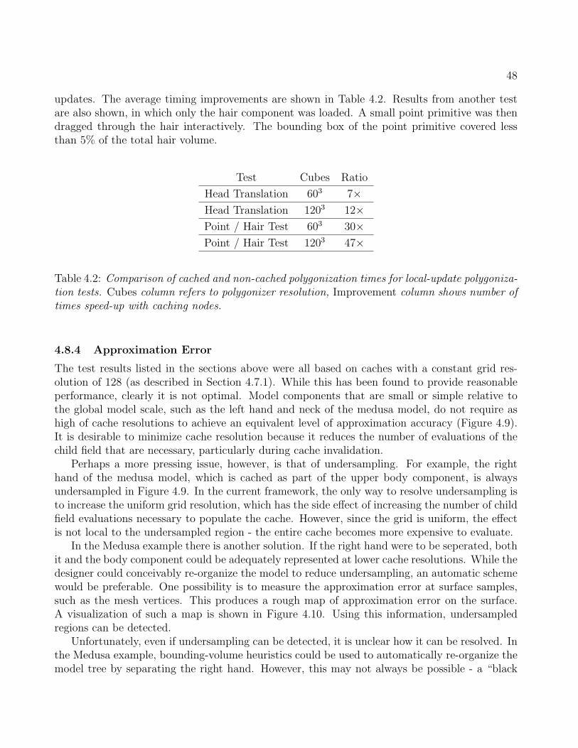
48

updates. The average timing improvements are shown in Table 4.2. Results from another testare also shown, in which only the hair component was loaded. A small point primitive was thendragged through the hair interactively. The bounding box of the point primitive covered lessthan 5% of the total hair volume.

Test Cubes Ratio

Head Translation 603 7×

Head Translation 1203 12×

Point / Hair Test 603 30×

Point / Hair Test 1203 47×

Table 4.2: Comparison of cached and non-cached polygonization times for local-update polygoniza-tion tests. Cubes column refers to polygonizer resolution, Improvement column shows number oftimes speed-up with caching nodes.

4.8.4 Approximation Error

The test results listed in the sections above were all based on caches with a constant grid res-olution of 128 (as described in Section 4.7.1). While this has been found to provide reasonableperformance, clearly it is not optimal. Model components that are small or simple relative tothe global model scale, such as the left hand and neck of the medusa model, do not require ashigh of cache resolutions to achieve an equivalent level of approximation accuracy (Figure 4.9).It is desirable to minimize cache resolution because it reduces the number of evaluations of thechild field that are necessary, particularly during cache invalidation.

Perhaps a more pressing issue, however, is that of undersampling. For example, the righthand of the medusa model, which is cached as part of the upper body component, is alwaysundersampled in Figure 4.9. In the current framework, the only way to resolve undersampling isto increase the uniform grid resolution, which has the side effect of increasing the number of childfield evaluations necessary to populate the cache. However, since the grid is uniform, the effectis not local to the undersampled region - the entire cache becomes more expensive to evaluate.

In the Medusa example there is another solution. If the right hand were to be seperated, bothit and the body component could be adequately represented at lower cache resolutions. While thedesigner could conceivably re-organize the model to reduce undersampling, an automatic schemewould be preferable. One possibility is to measure the approximation error at surface samples,such as the mesh vertices. This produces a rough map of approximation error on the surface.A visualization of such a map is shown in Figure 4.10. Using this information, undersampledregions can be detected.

Unfortunately, even if undersampling can be detected, it is unclear how it can be resolved. Inthe Medusa example, bounding-volume heuristics could be used to automatically re-organize themodel tree by separating the right hand. However, this may not always be possible - a “black

49

Figure 4.9: Medusa model with component cache resolutions of (left to right) 16, 32, 64, and 128.Even at very low cache resolution, the left hand component is represented adequately. In contrast,the right hand (which is part of the much larger upper body component) is undersampled evenat 128 resolution. Tri-quadratic value sampling is used at lower resolutions to increase surfacesmoothness.

Figure 4.10: Approximation error on the Medusa model. Mesh vertices are colored based on theabsolute difference between the approximated field value and the accurate field value. The colorscale runs from blue (low error) to green (high error). The images shown are (a) 1283 tri-linearreconstruction, (b) 1283 tri-quadratic, (c) 2563 tri-linear, and (d) 2563 tri-quadratic. Since (b)and (d) use approximation rather than interpolation, they have higher error than (a) and (c),which is clearly visible in these images.

50

box” tree node may contain small details that cannot be segmented. Alternatives here includeusing a multi-resolution cache with locally adaptive resolution, or simply by-passing the cache inthe undersampled region. Both these solutions are problematic. As described in Section 4.9.4,existing multi-resolution spatial caching schemes do not provide the C1 continuity required forsmooth surface visualization (Section 4.6). By-passing the cache introduces similar problems,and also may significantly reduce interactivity, since regions that are undersampled inconve-niently correspond to the expensive, high-detail portions of the model. A suitable approach toautomatically reducing undersampling has yet to be developed.

One final sampling issue involves sharp features. This problem was discussed in Section 4.6, a3D example is shown in Figure 4.11. While grid-based reconstruction can appear to reconstructsharp features if the sampling rate is high enough [49], the sharp edge is necessarily lost when moreclosely examined. Some polygonization algorithms attempt to resolve sharp features by searchingfor large changes in gradient direction at adjacent mesh vertices [121, 66, 76]. These algorithmsare quite effective when used with analytic gradients, as seen in Figure 4.11a. However, theyperform poorly with gradients reconstructed using tri-linear and tri-quadratic filters, becauseof regular C1 discontinuities in the former, and gradient smoothing in the latter. A variety ofrelated techniques have been developed for implicit surfaces based on point-set interpolation(Section 3.5). Currently, these methods are only designed to approximate creases in surfaces - itis unclear that they could be adapted to general scalar field approximation.

Figure 4.11: Comparison of representation of a sharp edge without caching (a), with a cacheresolution of 128 (b), and 256 (c). The Extended Marching Cubes polygnizer is used, producinga clear sharp edge in (a), but having no effect in (b) and (c) due to gradient smoothing at thecrease.

4.9 Spatial Caching with Adaptive Distance Fields

In the previous sections, spatial caching of a scalar field f(p) has been implemented using uniformgrids. Consider the case where f(p) represents a large surface which has very small details. Toaccurately represent the details, f(p) must be sampled very finely. This finely-sampled voxelgrid will require a significant amount of memory to store, but a more immediate problem forHierarchical Spatial Caching is that the cost of computing all the samples becomes prohibitive.

51

An improvement would be to adjust the sampling rate based on the size of the local details inthe scalar field. This local refinement process is commonly known as adaptive sampling.

Recently, Adaptive Distance Fields, or ADFs, have been proposed as a solution for adaptivesampling and approximation of distance fields [49]. In short, the uniform grid is replaced witha hierarchy of voxels known as an octree. For any particular cell containing the surface, anerror function is computed by comparing tri-linearly reconstructed values in the cell with realevaluations of f(p). If the error is too high, the cell is subdivided into 8 child cells. Subdivisionis repeated until the maximum error in all leaf cells is below some tolerance.

ADFs have been applied successfully to interactive modeling [83]. Frisken et al claim thattheir ADF techniques can be applied to general scalar field approximation, and hence should beusable in Hierarchical Spatial Caching. However, a detailed study has shown that this is not thecase.

4.9.1 Octree Subdivision

In [49],the following test is proposed to determine when to subdivide an octree cell. First, onlyoctree cells containing the surface are considered for subdivision. The value of f(p) is computedat 19 points - 12 samples at the middle of each cell edge, 6 at the center of each face, and one atthe center of the cell. These real values are compared with the approximate values (computed bytri-linear reconstruction based on the samples stored at the cell corners). The maximum error isthen compared with a global error tolerance, and the cell is subdivided if the estimated error istoo high.

One issue with this test is that only cells containing the surface are subdivided. The result isthat the distance field approximation becomes much less accurate further away from the surface(Figure 4.12). This poor approximation does not affect most ADF applications because the far-field is only used to determine inside-outside tests. However, the far-field is an integral componentof blending operators in BlobTree modeling. The poor far-field approximation causes blendingartifacts and hence is unnacceptable. All cells must be considered for subdivision, resulting ina significant increase in the size of the final ADF (Figure 4.12) These extra cells make dynamicconstruction of ADFs even more costly.

4.9.2 Dynamic Construction

Applications of ADFs largely assume that the ADF is pre-computed off-line. Interactive applica-tions interrogate the ADF data structure, and in some cases interactively combine two existingADFs [83] into a new ADF, but entire ADFs are not generated dynamically. However, hier-archical spatial caching enables interactive BlobTree manipulation precisely because the spatialcaches are created dynamically through lazy evaluation. Dynamic ADF construction has signif-icant overhead.

First, the subdivision tests described in the previous section require 19 samples of both theunderlying scalar field f and the current ADF, to determine whether the approximation errorin a cell is acceptable. Consider the case when the ADF octree is initially empty. Evaluatingthe ADF at a single point p will require dynamic expansion of the octree down to a sufficientlevel. Many 19-sample tests will be required. Compare this with evaluating a tri-linear cell

52

Figure 4.12: The ADF generated using Frisken et al’s technique of only subdividing surface cells(b) produces 1385 voxels, but poorly approximates the original distance field (a). Subdividingeverywhere (c) is visually more accurate but produces 7833 voxels, an increase of over 550%.

53

in a dynamic uniform grid. At most 8 samples of f will be computed. In theory, the cost ofoctree expansion is amortized when it is truncated at higher tree levels (where a larger cell isadequate). However, during interactive manipulation at lower polygonization resolutions, it isoften the case that only a few leaf cells in the update region will actually be necessary beforethey are invalidated. Hence, the octree expansion can introduce significant overhead.

The ADF error test also introduces extra overhead at leaf cells. Expansion continues untila leaf cell passes the error test, which requires 19 samples of f and the ADF. However, unlikeduring octree expansion, at a leaf cell these samples are not stored - they are discarded. Thisis a considerable expense. If the leaf cell is re-used many times than this expense amortized,but during interactive manipulation any leaf cells in the update region will be destroyed andre-generated each frame. Again, this is a significant overhead.

These construction costs are significant problems for any dynamic adaptive approximationscheme to be used in Hierarchical Spatial Caching. Approximation error is traditionally measuredby sampling, however the primary means for increasing interactive visualization speed is to avoidcomputing many samples! It may be possible to formulate error tests based entirely on existingsamples, by measuring values such as (approximated) curvature or gradient magnitude. Thiswould mitigate the overhead at leaf nodes. The adaptive expansion overhead is more challenging.One possible approach is to replace the global octree with a uniform grid of cells which arethemselves octrees. If the uniform grid resolution were adequate, only the octree-cells in higher-detail regions would be expanded beyond the root node. However, determining a suitable uniformoctree-grid resolution is problematic. Note that this approach also solves the expansion problem.

One objection to these statements is that the Kizamu system [83] supports interactive editingof ADFs, by using the ADF of a “carving tool” to add or subtract from the exising ADF. However,the demonstrated examples in [83] generally show carving of small details on a large surface. Itis not clear that large-scale editing operations are interactive. Second, Kizamu only supportsbinary CSG compositions. Visually, CSG operations are simply a composition of two surfaces,so Kizamu only updates the ADF within the visual bounding box of the tool. This is notacceptable in a BlobTree modeler, the entire support region of the tool’s scalar field must beupdated. Finally, as noted in section 4.9.1, ADF subdivision only occurs in cells containingthe surface. The additional octree expansion (Section 4.9.1) required for accurate scalar fieldapproximation is avoided.

4.9.3 Sampling Cost

The entire purpose of hierarchical spatial caching is to reduce the cost of sampling f . The moreefficient a spatial cache is to sample, the more interactive the modeling system will be. Hence,it is important to consider the cost of sampling an ADF.

ADF’s apply the tri-linear filter to reconstruct the distance field approximation at a pointp. This filter is ideal for the octree data structure, as only the 8 corner samples of the leaf cellcontaining p are required. However, finding the leaf cell requires O(log N) steps. Frisken etal [50] optimize this leaf search by replacing the standard recursive algorithm with an iterativealgorithm, however O(log N) iterations are still required. After the leaf cell is found, the 8 cornervertices are located through indirect hash-table lookups - at best an amortized O(1) cost.

54

In comparison, the blocked uniform grid scheme described in section 4.7.3 supports directlookup of the bottom-left corner of the cell containing p. In the best case, all the necessaryvalues are stored in a single contiguous block which (if properly sized) fits entirely in a CPUcache line. In the worst case, each necessary value is in a separate block, however these valuesare located directly by indexing into the separate blocks. The total cost is significantly lowerthan the O(log N) octree traversal and 8 hash table lookups necessary for an ADF.

4.9.4 Continuity

The issues with ADFs described thus far have all been related to computational constraints, whichin the future may become less restrictive. However, a more fundmental problem with ADFs isthat the scalar fields generated by ADFs are not C0 continuous. As noted in Section 2.6, C0

continuity is a requirement for consistent implicit modeling.Consider the simplest case in 2D, where the neighbour of cell A is subdivided once (Fig-

ure 4.13). In cell A, the value at the midpoint of the edge between values a and b is obtainedby linear interpolation. However, in the adjacent cells, the value at the midpoint of edge E isone of the stored “true” samples of f . If f is not linear along this edge, a C0 discontinuity willnecessarily exist in some neighbourhood of E. For most f , the discontinuity will exist along theentire edge. These discontinuities are clearly visible in Figure 4.12. As explained in Section 2.6,C0 discontinuities result in holes in the surface, and hence ADFs are incompatible with the basicscalar field requirements for implicit modeling.

Figure 4.13: C0 discontinuty between octree cells.

4.10 Chapter Summary

The interactive visualization problem has prohibited the use of hierarchical implicit modelingsystems such as the BlobTree in interactive shape modeling tools. In this chapter, an approachhas been developed for improving interactive visualization times. Hierarchical spatial cachingcombines aspects of existing caching schemes, namely traversal caching and spatial caching, toreduce the cost of evaluating internal branches of a BlobTree model from O(N) to O(1). Thisnovel technique results in an order-of-magnitude improvement in visualization time. A varietyof implementation options have been discussed, as well as several optimization techniques usedin the testing implementation.

In an attempt to reduce approximation error, the octree-based Adaptive Distance Field tech-nique was investigated for use in hierarchical spatial caching. Unfortunately, no viable approachwas found. It is clear that interactive construction of ADFs has significant computational costs

55

which have yet to be addressed. Finally, and most conclusively, the lack of a C0 reconstructionscheme prohibits the use of octree ADFs for representation of valid implicit volumes.

One possible way forward may be to move to multiple partition-of-unity (MPU) schemes,such as the MPU-RBF [87] approach. Currently, these methods are not designed for interactiveconstruction, have a relatively high sampling cost, and an expensive error metric. If these issuescan be addressed, MPU approximation schemes may be usable as a drop-in replacement forregular sampling in hierarchical spatial caching.

Chapter 5

Implicit Sweep Surfaces

BlobTree-compatible implicit sweep objects are developed which support direct specification andmanipulation of the surface with no topological limitations on the 2D sweep template. A 2Ddistance field approximation technique is described which is C2 smooth except at sharp creases,and is easily converted to a bounded field. Several sweep endcap techniques are introduced, andseveral applications are considered.

Some material in this chapter is taken from the publication “Generalized Sweep Templates forImplicit Modeling” by Schmidt and Wyvill [96]. The material appearing here is due to Schmidt.

5.1 Implicit Sweep Surfaces

Sweep surfaces, nearly ubiquitous in parametric modeling for the last 20 years [85], are a usefulinteractive modeling metaphor. However, sweep surface methods are very limited in the hierar-chical implicit modeling domain [27]. Existing implicit sweep representations compatible withthe BlobTree are limited to star-shape sweep profiles defined by offset curves [37]. Implicit sweeptechniques that support the intuitive direct profile manipulation available in the parametricdomain have not been previously developed for the BlobTree.

One of the key problems regarding implicit sweeps is the definition of a suitable 2D sweeptemplate scalar field. In the parametric domain a sweep surface is generated by sweeping a 2Dtemplate curve C along a 3D trajectory T . In the implicit domain, a 2D template scalar fieldfC must be created which represents C and can be swept along T . To create well-defined 3Dvolumes, C must be a closed contour. Also, fC should be bounded and continuous if the scalarfield created by sweeping fC is to be used in the BlobTree. In particular, gradient discontinuitiesin the field away from the surface must be avoided to prevent blending artifacts.

In this chapter, a technique is described for generating 2D sweep template fields that can beused to create sweep volumes which have good blending properties and are compatible with theBlobTree (Section 5.3). First, a simple technique is described for converting distance fields tobounded fields, allowing any set of closed 2D contours, including nested “hole” contours, to beused to create an implicit sweep template. Then, existing variational curve-fitting techniques areextended to create a distance field approximation which is C2 away from the surface, providinggood blending properties, but preserves creases in the sweep template contour.

The approach to used to sweep the template scalar field largely follows classical methods(Section 5.4). One issue which has not been previously discussed is the generation of differentsweep endcap styles. Three novel sweep endcap styles are described - flat endcaps with sharpand rounded edges, and a smooth variable-width endcap.

The goal of this sweep formulation is to create implicit sweep volumes compatible with theBlobTree. Within this framework, implicit sweeps can be composed with other implicit volumes

56

57

(including other implicit sweeps). These sweep primitives have been implemented in an inter-active BlobTree modeling environment (Chapter 6). To reduce evaluation time in interactivecontexts, the sweep template fC is discretely approximated (Section 5.6).

Since C is directly approximated by fC, the resulting implicit sweep surfaces are nearly iden-tical to parametric sweep surfaces created by sweeping C (Section 5.7). The implicit formulationtransparently handles difficult degenerate cases, such as self-intersecting sweeps (Section 5.5),that are problematic in the parametric formulation. In addition, parallel contours representedimplicitly can simply be interpolated to reconstruct 3D surfaces (Section 5.8).

In interactive contexts, the ability to directly manipulate the surface contour is much moreefficient than the previous offset-contour methods. The interaction techniques developed forparametric sweeps can be used without modification. Combined with their good blending be-havior, the implicit sweep primitives developed in this chapter are an intuitive and expressivefree-form addition to BlobTree modeling.

5.2 Previous Approaches

Solid modeling by sweeping a 2D area (commonly referred to as a sweep template) along a 3Dtrajectory is a well known technique in computer graphics [85, 47]. Most early CAD systems [86]supported sweep surfaces as boundary representations (B-reps). These B-rep sweep solids lackeda robust mathematical foundation, self-intersecting sweeps were simply invalid. Recent workon the more general problem of sweeping a 3D volume has produced several general swept-volume envelope computation techniques which employ either the sweep-envelope differentialequation [23] or Jacobian rank-deficiency conditions [3]. Applications of these techniques areexplored in a recent survey [1]. These methods operate on closed-form boundary representationswhich are symbolically manipulated. The volume boundaries can be defined using closed-formimplicit surfaces [2]. However, the resulting swept volume is still a boundary representation,and not an implicit volume defined such as in Equation 2.3. Sourin et al [108] describe atechnique for sweeping implicit volumes. Evaluating the resulting function requires slow non-linear optimization algorithms.

There are essentially two approaches to creating implicit sweep surfaces. One method isto convert the 2D sweep template to a 2D scalar field, and then sweep this scalar field in 3D.Alternatively, a discretization of a 3D parametric sweep surface (such as a triangle mesh or pointset) can be approximated with an implicit representation.

Creating an implicit representation of an arbitrary 3D surface is non-trivial. Some success inthis domain has been achieved using scattered-data interpolation techniques, where an implicitsurface is defined that passes through a set of 3D sample points. One approach, variationalimplicit surfaces [113, 92], involves solving a dense matrix and hence does not scale to more thana few thousand sample points - insufficient to adequately represent a complex sweep surface.The cost of solving the linear system can be greatly reduced using Fast Multipole Methods,permitting millions of sample points to be used [34]. Unfortunately the multipole expansionsnecessary to implement this technique were not provided in [34] and have not been published.In addition, these approximation techniques cannot represent sharp creases or points, since the

58

variational implicit surface is globally C2 continous. Interpolation of point values is generalized inthe concept of transfinite interpolation [91], which can interpolate arbitrary geometric curves andpreserves discontinuities. However, this technique has only been demonstrated for a restrictedset of closed-form 2D implicit contours.

Another class of scattered-data interpolation techniques have been developed that employbasis functions with local support [72]. The underlying linear systems are sparse and hencemore efficient to solve. Partition of unity techniques such as MPU implicit surfaces [75] andthe Partition of Unity Variational method [87] apply hierarchical approximation techniques tosimplify surface fitting and can represent sharp features in certain configurations. However, thesetechniques are not guaranteed to define an implicit volume (Equation 2.3). Additional internaliso-surfaces may be produced as a result of blending local approximations with finite support [87].Volume modeling operations such as CSG may expose these internal iso-surfaces. The ImplicitMoving-Least-Squares (IMLS) technique [105] converts triangle meshes into implicit volumes andhence could be used to define implicit sweep surfaces. However, the implicit surface interpolatesthe tessellation - the differential properties of the sweep template are lost, local curvature isalways zero (or infinite on the creases between each triangle), and an adequate tessellation levelmust be determined.

[102] and [116] approximate sweep surfaces with volume datasets. The sweep dataset isinitialized by sampling a sweep template specified as a 2D image. Volume datasets cannotrepresent features smaller than a single voxel. Surface creases and sharp points are also lost inthe conversion process. Adaptively-Sampled Distance Fields (ADFs) [49] attempt to deal withthese issues, but contain C1 discontinuities in the reconstructed scalar field.

Implicit sweeps can alternatively be defined by following the parametric approach of sweepinga 2D template. One key issue is the definition of a suitable implicit template. A 2D scalar fieldmust be defined that represents the closed 2D template contours. This scalar field is then sweptalong the sweep trajectory.

[37] describes implicit sweep primitives with bounded sweep template fields. Profile curvesdefined in polar coordinates are used to create an anisotropic distance field. The sweep surfaceis an offset surface from the swept profile curve, prohibiting direct surface specification. Profilecurves are limited to “star-shapes” by the polar definition. [55] describes implicit generalizedcylinders which have a similar limitation.

Another approach is to approximate the contour with a polygon, and then construct an im-plicit representation of the polygon [80, 17]. These methods require that non-convex polygons becarefully decomposed into pieces that can be properly combined using CSG intersection opera-tions. This decomposition is non-trivial. The properties of the resulting scalar field are dependenton the tessellation level (Figure 5.1d). These issues can be mitigated using explicit normalizationtechniques [22]. A side-effect of this normalization is that offset iso-contours quickly converge toa circle (Figure 5.1e). While Huygen’s Principle guarantees that all distance fields will convergeto circular iso-contours in the limit, in this case it happens quickly and has an undesirable effecton blending.

A swept 2D implicit polygon results in a faceted 3D sweep surface. Curvature at the surfaceis not preserved, and gradient discontinuities exist along the sweep paths of each vertex in the2D polygon. The 2D polygon can be smoothed at the vertices [81]. However, this “corner-

59

cutting” reduces the accuracy of the approximation as the surface no longer passes through theaccurate surface samples (the polygon vertices). An implicit representation of 2D curves has beendescribed [80], but is based on an underlying “carrier polygon” that has only been developedfor cubic polynomial splines. Variational interpolation can also be applied to approximate a 2Dcontour [125]. The standard technique involves constraining the variational solution only nearthe contour, the rest of the field is unconstrained and hence determining bounds is very difficult(Figure 5.1c).

2D implicit curves can be represented using level set techniques [77]. These algorithms arebased on 2D pixel discretizations, and hence have the same issues as volume datasets regardingsmall and sharp features. Skeletonization techniques such as Medial Axis Transform [30] can beused to compute distance fields which approximate curves but also contain C1 discontinuities.

To summarize, several implicit sweep models have been proposed that support direct surfacespecification and manipulation. However, none of these models produce the bounded scalar fieldsnecessary for interactive modeling of complex hierarchical implicit models [120, 97].

Figure 5.1: Scalar fields generated from contour (a), with filter (1 + sin(k · f))/2 applied to thefield before mapping to grayscale to emphasize iso-contours. Red highlight indicates region insidecontour, blue highlight indicates bounded region after applying Equation 2.12. Exact distance field(b) has C1 discontinuities inside contour. Variational approximation (c) using normal constraintsprovides a poor approximation to (b). Approximation with a C1 implicit polygon (d) is sensitiveto the tessellation of the curve, field values grow as tessellation level is increased. A normalizedimplicit polygon (e) is accurate near the contour, but the iso-contours quickly tend to a circularshape. The variational approximation with boundary constraints proposed in this chapter (f)closely approximates (b) inside the falloff region but is globally C2 continuous.

60

5.3 2D Implicit Sweep Templates

In the following section a method is developed for creating a 2D implicit sweep template whichrepresents a closed 2D contour C. First, a technique for converting the signed distance field dC

to a bounded 2D field is described. This simple method allows BlobTree-compatible implicitsweep surfaces to be generated from any set of closed 2D contours. Then, a method is developedfor creating a smooth approximation dC to the exact distance field dC which does not containundesirable C1 discontinuities. This approximation technique, which is based on existing workwhich approximates curves using variational interpolation [113], cannot reproduce sharp edges inC. To mitigate this problem, a technique for re-introducing sharp edges into the sweep templateis described, followed by a comparison of the distance field approximation with existing methods.

5.3.1 Bounding Distance Fields

The approach used to create skeletal primitives - applying gw (Equation 2.12) to a distancefield - can be adapted to create the sweep template field fC. In the distance field dC the curvelies on the zero iso-contour, dC = 0. If gw is applied directly to dC, the iso-contour defined bygw ◦ dC = viso 6= 0 will be offset from C. As noted above, sweeps generated by offset iso-contoursgenerally do not support direct manipulation and hence are difficult to control. To force thiscontour to lie on C the distance values must be shifted. First, dC must be converted to a signeddistance field, where points inside C have a negative distance value (Section 2.2). The shifteddistance d′

C is then:d′

C = min(g−1w (viso) + dC, 0) (5.1)

The bounded 2D sweep template field fC is then defined as

fC = gw ◦ d′

C (5.2)

To give some sense of what this equation accomplishes, consider Figure 5.2. When a potentialfunction is applied to the distance field of a standard skeletal primitive, such as the line in 5.2a,an offset curve is produced. For sweeps, this final curve is known, and the task is instead to finda skeleton which would generate the desired offset curve, as shown in 5.2b. However, this is notalways possible. Curves with sharp edges, such as the rectangle in 5.2c, cannot be generatedby a constant-offset curve from any skeleton, since constant-offset curves always round off sharpconvex edges, as shown in 5.2d. Equation 5.1 avoids this difficulty by directly generating ascalar field with the desired iso-contour. Hence, a skeleton is implicitly defined by this equation -however, the input curve is not necessarily a constant-offset from this skeleton (as in Figure5.2c).

Since C may be non-convex, dC can contain C1 discontinuities (Figure 5.4a), and hence sowill the bounded field fC (Section 2.7). These discontinuities will be swept in 3D and produceundesirable blending artifacts (Figure 2.6a). To avoid this problem an approximation to dC mustbe developed which has a smooth field away from the surface.

5.3.2 C2 Distance Field Approximation

An implicit approximation to a 2D contour C can be created using variational interpolation [113].A C2 interpolating thin-plate spline is fitted to a set of constraint points placed at samples of C.

61

Figure 5.2: Skeletal primitives, such as the line in (a), generate offset contours (shown inmagenta). Equation 5.1 implicitly defines the “skeleton” area for an arbitrary curve, as shownin (b). However, the skeleton defined for the curve in (c) could not be used to directly re-producethe curve, as the offset contour smooths out convex corners.

To adequately constrain the solution, normal constraints [34, 125] are added. Inner and outernormal constraints at a sample point are added at short distances along the normal to C at theon-curve sample (Figure 5.3a).

Normal constraints only ensure that the iso-contour passes through the sample points. Thescalar field is unconstrained further from the surface, resulting in a poor approximation to thedistance field (particularly in the case of non-convex C, see Figure 5.4). This is especially prob-lematic if the resulting function is to be bounded, since it is non-trivial to determine the boundingregion of the non-zero field values without resorting to a time-consuming spatial search.

Figure 5.3: Normal constraints (a) at a point ci are added at short offset M s from the curve C,along the curve normal ni. Boundary constraints (b) are placed at a constant distance from C toimprove the distance field approximation and ensure that the field fC is bounded within a knowndistance.

Variational approximation produces an implicit curve, rather than polygon. Since only sam-ple points are necessary, there are no restrictions on C. However, normal constraints alone areinsufficient to produce a variational solution which approximates a distance field. To constrainthe variational solution in regions further from the curve, boundary constraints are added (Fig-ure 5.3b).

Boundary constraint points are generated by sampling several iso-contours of the distancefield. A reasonable distance field approximation can be obtained using one set of boundary

62

constraints along the iso-contour found at a distance of g−1w (0). After applying gw, this contour

bounds the non-zero field values, and hence can be used to determine a bounding region. In theexamples shown in this section, two additional iso-contour constraints have been used, one atg−1

w (0.5 ∗ viso), which is approximately half-way between C and the zero-contour, and another atg−1

w (1.5 ∗ viso), which lies inside C. The purpose of these extra constraints is to further reduceerror in the distance field approximation.

If C has high-frequency features, there may be higher error in the distance field approximationclose to the curve. In interactive modeling with implicit sweeps, this error is not particularlycritical. However, the situation can be identified automatically by comparing approximateddistance values with exact distance values at small offsets from C. If the measured error isunacceptable, several directions can be taken. The first is to increase sampling density along theexisting iso-contour constraints. In practice, sampling each iso-contour constraint with between50 and 100 uniformly-spaced sample points produced satisfactory results in all test cases. Forcurves with very small features, higher sampling rates, or non-uniform importance sampling, maybe necessary. To further reduce approximation error, additional sets of iso-contour constraintsclose to C can be inserted.

Tracing iso-contours in the exact distance field dC is non-trivial and computationally inten-sive. To accelerate computation, dC is approximated on a discrete 2D grid using a distancetransform [61] algorithm. Approximate iso-contours can then be efficiently extracted from thedistance transform. The test implementation uses the CSSED algorithm which runs in lineartime in the number of image pixels [38]. The distance transform is computed on a 5122 pixelimage and then discrete iso-contours are traced in the image. The resolution here is not critical,similar results have been found with 1282 pixel images.

Alternatives to this iso-contour-sampling technique have been found to produce unsatisfactoryresults in limited testing. Since the variational solution minimizes global curvature, constraintsbased on either random or regular sampling can result in unexpected oscillations. In addition,regular sampling introduces many spurious constraint points and if the sampling frequency istoo high the discontinuities in the distance field are closely approximated. When these high-frequency areas are blended, the perceptual discontinuities described in Section 2.8 can occur.In theory, this problem can also occur with the iso-contour sampling described above, since iso-contours in the distance transform approximate the non-C1 iso-contours in the distance field.This problem can be avoided by replacing the distance transform with a fast-marching level setmethod that propagates at curvature-dependent speeds [77]. The discrete iso-contours producedby this algorithm smooth out the C0 discontinuities in the distance field, minimizing the chancethat perceptual discontinuities will be introduced.

Adding boundary constraints to the variational solution results in a much more accurateapproximation to the distance field, particularly in the case of non-convex curves (Figure 5.4).The variational scalar field is a globally C2 continuous approximation to dC.

5.3.3 Sharp Features

The variational approximation to C is globally C2 continuous. This implies that sharp features,which are C1 discontinuities in C, are not preserved in the variational approximation. Significant

63

Figure 5.4: Scalar fields generated using a non-convex curve (a). The exact distance field (b)has C1 discontinuities inside and outside the curve. Approximation with a normalized implicitpolygon (c) and variational approximation with normal constraints (d) provide poor approxima-tions in concave region. Our approach (e) smoothly approximates the distance field away fromthe surface.

smoothing can be observed near creases, even with very high sampling rates (Figure 5.5a). Creaseapproximation can be improved by using anisotropic basis functions [43] but these basis functionsstill do not create sharp C1 discontinuities. Sharp features are preserved with implicit polygontechniques [22, 17]. To re-introduce sharp features into the constrained variational approacha constructive approach is taken which incorporates these existing techniques. The C2 smoothdistance field approximation described above is used for most of the field, however in a smalldisc around sharp features, a crease-preserving implicit polygon approximation dC is used. Topreserve continuity, these fields are blended in a transition region around each feature region.

A set of crease positions ci are assumed to be known, as is a feature radius ri. When evaluatingfC at a 2D point u, the distance k from u to the nearest feature point is computed. The blendeddistance field approximation d?

C is then defined as follows:

d?C =

dC if k ≤ r

(1 − gw(kr))dC + gw(k

r)dC if r < k < 2r

dC if k ≥ 2r

(5.3)

See Figure 5.6 for a graphical representation of the blending regions. The use of gw here isnot significant, any smooth interpolating function can be used. This method is similar to thebounded-blending techniques used to control implicit volume composition operators [82, 52]. Anexample is shown in Figure 5.5.

In the examples shown, the normalized implicit polygon approach [22] is used to define the

crease-preserving field dC. The necessary equations are described in Appendix B. To locatecrease points on C, the rudimentary method of thresholding the angles between consecutiveline segments in the polygonal approximation is used. This technique is not robust but worksreasonably well for most creases.

This blending approach provides the benefits of boundary-constrained variational approxi-mation while also locally preserving sharp features. Since this method provides a more accuratedistance field approximation (Figure 5.1), it may be more appropriate than implicit polygon ap-proaches even when C is actually a polygon. However, there are some drawbacks. In the blending

64

Figure 5.5: The boundary-constrained variational method described in section 5.3.2 rounds outsharp edges (a) because it is globally C2 continuous. Sharp features can be re-introduced (b) byblending between an implicit polygon and the variational field in the feature regions (see sec-tion 5.3.3).

regions around feature points the scalar field may not be monotonic, since the two fields beingcombined can be increasing at different rates. As previously noted, curvature in the featureregion is not preserved by the polygonal approximation.

Figure 5.6: A scalar field dC that preserves sharp features in C can be combined with a smoothapproximation dC. Within a distance r from the sharp feature, dC is used. Outside the radius 2r,dC is used. Between r and 2r (dashed circles in diagram), dC and dC are smoothly blended.

5.3.4 Analysis

A variety of implicit representations for general 2D curves have been developed (Section 5.2).The scalar fields generated by some of these techniques are compared in Figures 5.1 and 5.4.In both of these examples it is clear that the technique described in this section more closelyapproximates a distance field than existing methods. Close approximation to a distance fieldis desirable because it allows easy computation of field bounds and results in more predictable

65

blending behavior. The technique used to generate Figure 5.1d, for example, is sensitive to thetessellation level of the curve. If the tessellation level is increased, the iso-contour spacing willchange and hence blend surfaces will also change. This is unacceptable. The normalized polygonapproach [22] does not have this problem; however, the iso-contours produced approach a circularshape very quickly (Figure 5.4c). This results in undesirable blending behavior (Figure 5.7). Inboth of these cases, the scalar field represents a polygon, not a curve. The curvature of the inputcontour C is lost, and hence the differential surface properties of the implicit sweep do not reflectthose that would be computed with a parametric sweep. Although it is still an approximation,the variational sweep template produces a smooth curve and hence approximates the curvatureof the accurate sweep surface.

Figure 5.7: Implicit sweep blended with cylinder. Sweep template is computed using normalizedimplicit polygon in (a), and boundary-constrained variational approximation in (b). Black lineshows edge of non-blended cylinder, dashed red line in (b) shows outline of (a). Blending in (b)is more localized and has a softer transition.

Defining “goodness” measures for distance field approximation is challenging. One test is tocompare the approximated field values with the exact distance field values. However, since thewhole point of distance field approximation is to avoid the discontinuities that occur in the exactdistance field, zero error is in fact undesirable. Still, this test has been performed with a variety ofconvex and non-convex curves. On average, variational curves with boundary constraints reducethe mean error by a factor of 25 over the normalized implicit polygon approach.

As noted in Section 2.9, distance fields are normalized (|∇f | = 1 everywhere except along thediscontinuity curves). Again, if the goal is to smooth discontinuities in a distance field, minimizingthe gradient magnitude error |1 − |∇f || is undesirable as it will produce high-frequency C2 regionsthat are effectively perceptual discontinuities (Section 2.8). However, this is still a useful errormetric because near-normalization is a desirable property. Variational curves with boundaryconstraints have a mean normalization error that is on average a factor of 4 lower than theimplicit polygon approach.

Normalization images (Section 2.9.1) are a useful tool for visually inspecting the normaliza-tion error over a field. Two normalization images are shown in Figure 5.8. In both cases, the

66

normalization error is highest along what would be discontinuities in the exact distance field (in-side C, the discontinuities lie on the medial axis). In the implicit polygon approach (Figure 5.8a),the error is very low near C but increases rapidly away from the curve. The variational curvewith boundary constraints has somewhat higher error near C but is much more accurate insidethe bounded approximation region further from the curve.

Figure 5.8: Gradient images computed by mapping |1 − |∇f || to grayscale (white is maximumerror). Normalized implicit polygon (a) has low error near surface, but higher error than theboundary-constrained variational technique (b) in regions further from the surface.

5.4 Sweep Primitives

An implicit sweep primitive is defined by a 2D sweep template field fM (Equation 5.2) and a 3Dsweep trajectory T , which is assumed to be a parametric curve defined by one parameter:

T (s) = (tx(s), ty(s), tz(s)), 0 ≤ s ≤ 1

The sweep surface S is defined by a 3D scalar field fS . Given a point T (s) on the sweeptrajectory, a geometric transformation F(s) can be defined which maps 2D points u to 3D pointsp. F(s) is assumed to be affine and maps the 2D origin to T (s), implying that points F(s) · uare co-planar (Figure 5.9).

In the following discussion, 0 is appended as the third coordinate when converting 2D pointu to 3D point p. Going from 3D to 2D, the third coordinate is simply dropped. Application ofthis conversion will be determined by context and not explicitly denoted.

A possible definition for fS is:

fS(p) = fM(u), F(s) · u = p (5.4)

Unfortunately, given only a point p this equation cannot be directly evaluated because theparameter value s and 2D point u are unknown. Since F(s) is affine the inverse mapping F−1(s)can be computed:

fS(p) = fM(u), u = F−1(s) · p (5.5)

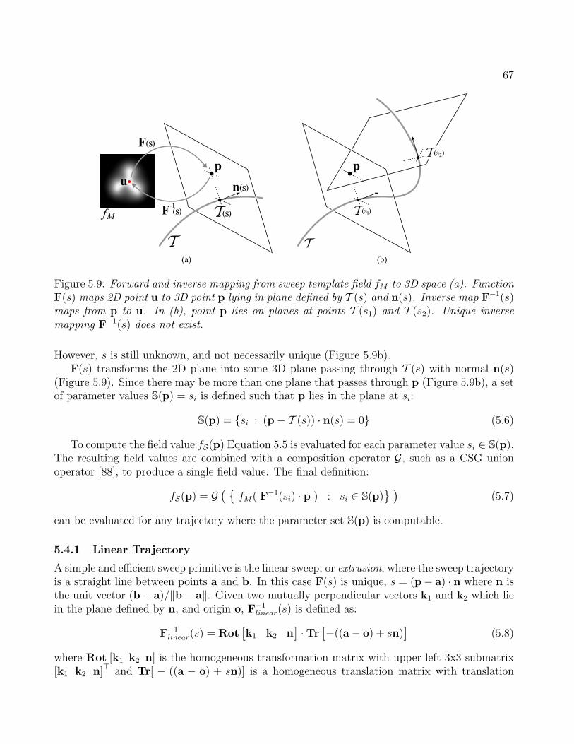
67

Figure 5.9: Forward and inverse mapping from sweep template field fM to 3D space (a). FunctionF(s) maps 2D point u to 3D point p lying in plane defined by T (s) and n(s). Inverse map F−1(s)maps from p to u. In (b), point p lies on planes at points T (s1) and T (s2). Unique inversemapping F−1(s) does not exist.

However, s is still unknown, and not necessarily unique (Figure 5.9b).F(s) transforms the 2D plane into some 3D plane passing through T (s) with normal n(s)

(Figure 5.9). Since there may be more than one plane that passes through p (Figure 5.9b), a setof parameter values S(p) = si is defined such that p lies in the plane at si:

S(p) = {si : (p − T (s)) · n(s) = 0} (5.6)

To compute the field value fS(p) Equation 5.5 is evaluated for each parameter value si ∈ S(p).The resulting field values are combined with a composition operator G, such as a CSG unionoperator [88], to produce a single field value. The final definition:

fS(p) = G( {

fM( F−1(si) · p ) : si ∈ S(p)} )

(5.7)

can be evaluated for any trajectory where the parameter set S(p) is computable.

5.4.1 Linear Trajectory

A simple and efficient sweep primitive is the linear sweep, or extrusion, where the sweep trajectoryis a straight line between points a and b. In this case F(s) is unique, s = (p− a) · n where n isthe unit vector (b− a)/‖b− a‖. Given two mutually perpendicular vectors k1 and k2 which liein the plane defined by n, and origin o, F−1

linear(s) is defined as:

F−1linear(s) = Rot

[k1 k2 n

]· Tr

[−((a − o) + sn)

](5.8)

where Rot [k1 k2 n] is the homogeneous transformation matrix with upper left 3x3 submatrix[k1 k2 n]> and Tr[ − ((a − o) + sn)] is a homogeneous translation matrix with translation

68

component −((a − o) + sn). Twisting and scaling can be introduced into the sweep surface byvarying k1 and k2 along the trajectory.

The linear sweep scalar field flinear is then defined as

flinear(p) = fM

(F−1

linear(s) · p)

The function flinear defines an scalar field of infinite extent along n which must explicitly bebounded to cap the ends of the sweep surface. The field should extend for some distance dendcap

beyond the sweep line endpoints to permit blending. It is desirable to have some control overthe endcap shape. Existing implicit sweeps create endcaps by linearly interpolating the sweeptemplate values to zero [37]. Three alternative endcap styles are now defined.

Flat Endcap With Sharp Transition An infinite linear sweep can be capped with flatendcaps by computing the Boolean intersection of the sweep with a rectangular box. Barthe’s[19] C1 intersection operator creates a sharp edge on the cap while still preserving C1 continuity.To optimize computation, the rectangular box can be replaced with two infinite planes. Notethat the intersection operator must be applied to the entire sweep to preserve continuity. Hence,between the infinite planes (in the sweep region) a field value of 1 is used. In Figure 5.10 aflat endcap created using this method is compared with one created using Ricci’s intersectionoperator [88], which creates C1 discontinuities

Figure 5.10: Flat endcap with sharp transition. C1 discontinuity on surface produces sharp crease(left) but does not propagate away from the surface with Barthe CSG intersection (middle). Ricciintersection produces C1 discontinuity away from surface (right). Isocontour is marked in red.

Flat Endcap With Smooth Transition An alternative to the sharp endcap above is to a flatendcap with a smooth transition region. Hybrid C1 CSG/blending operators that smooth outthe CSG transition zone but are otherwise identical to sharp CSG operators are defined by [19].Intersection with infinite planes is again used to smoothly transition from the sweep surface toa flat endcap. The size of the transition zone is controllable, Figure 5.11 shows endcaps withvarying parameter values. This operator converges to a C1 field discontinuity as the transitionzone size decreases.

Blobby Endcap A third style of endcap is related to the linear interpolation to 0 used inprevious approaches. Essentially, the goal is to scale flinear down to zero at some distance

69

Figure 5.11: Flat endcap style with smooth transition. Transition parameter varies from left toright 30◦, 35◦, 40◦. Rightmost image shows scalar field for 35◦ parameter. Isocontour is markedin red.

beyond the end of the sweep. Instead of linear interpolation, a smoother interpolating functionis used - in this case, gw (Equation 2.12). This function is applied to the distance past the end ofthe sweep, and used as a scaling factor for the field value flinear. A parameter dendcap determinesthe extent of the field beyond the end of the sweep line. If the parameter value at the lineendpoint is smax, the function in the endcap region is:

fendcap(p) = gw

(|s| − smax

dendcap

)· flinear(p) (5.9)

Field continuity is preserved by the zero tangents of gw. Because the value of flinear increasesas the interior distance from C increases, the field takes “longer” to reach zero at points furtherfrom the C. The result is an endcap with variable width (Figure 5.12). This variable widthprimitive with a free-form contour has been found to be extremely useful in interactive sketch-based modeling contexts (Section 6.4).

Figure 5.12: Blobby endcap style. Sweep profile (left) determines width of endcap at each point(middle). Width is dependent on field value inside the profile (right). Isocontour is marked inred.

5.4.2 Circular Trajectory

Circular sweep trajectories, described by a point o and a normalized axis n, result in surfaces ofrevolution. Several restrictions are necessary to provide an implicit circular sweep definition that

70

is valid for any trajectory and sweep template. The sweep function, Equation 5.7, cannot beevaluated at points lying on the axis n because the set S(p) (Equation 5.6) is infinite. To definecircular sweeps a simplifying assumption is made - that the template orientation and scaling isconstant. Under this constraint the infinite parameter set maps to a single point u.

Since twisting and scaling is disallowed, it is possible to compute point u in the sweep templatecorresponding to a point p without finding the angle θ on the circular trajectory. The 2Dcoordinates are found geometrically:

uy = (p − o) · n

ux = ‖(p − o) − uyn‖

The 2D coordinates corresponding to the opposing side of the circle are (−ux,uu). These samplepoints result in two field values which can be composed with a C1 union operator [19] to producea gradient-continuous scalar field.

Note that ux ≥ 0, implying that the portion of the sweep template to the left of the axis ofrevolution never sampled. This can be desirable as it is analogous to revolving an open curvearound an axis between the curve endpoints. Unfortunately it also produces a C1 discontinuityat points on n where fM is not continuous C1 continuous across the Y axis.

Open sweeps (sweeps along some arc segment of a circular curve) can be created by computingthe sweep angle [116] and applying the linear-sweep endcap techniques. Also, if the axis ofrevolution lies outside the bounds of fM , twisting can be safely applied, although for full circularsweeps the twist angle needs be a whole multiple of 2π to avoid C0 discontinuities. A similarrestriction applies for scaling.

5.4.3 Cubic Bezier Trajectory

As an example of a general trajectory, consider a 3D cubic Bezier curve B(s), s ∈ [0, 1]. As-sume that the normal function n(s) (Equation 5.6) is the tangent vector B′(s). The followingpolynomial in s must be solved to find the parameter value set S(p):

(p − B(s)) · B′(s) = 0 (5.10)

This polynomial is degree 5 for a cubic Bezier curve, precluding analytic solution. Numericalroot-finding techniques such as [100] must be used to solve for the roots s.

Once S(p) is computed, F−1bezier(s) can be evaluated:

F−1bezier(s) = Rot

[k1 k2 B′(s)

]· Tr

[−B(s)

]

Care needs be taken when defining the vectors k1 and k2. One option is to calculate the Frenetframe [47]:

k1 = B′(s) × B′′(s)

k2 = k1 × B′(s)

However B′′(s) = 0 in degenerate cases such as straight sections. The Frenet frame can also flipdirection across points of inflection, creating C0 discontinuities. An alternative is the rotation

71

minimizing frame of [25]. This frame is procedurally defined based on an initial frame at B(0)and cannot be calculated analytically. In order to generate a frame at any s, a table of rotationminimizing frames Fj can be calculated at points sj along the curve. F−1

bezier(s) is then found bylocating the nearest sj < s and computing a rotation minimizing frame from Fj. This techniqueis known as Bishop framing [21].

The cap styles described in Section 5.4.1 are all applicable to arbitrary curved trajectories.Twisting and scaling can also be applied based on s or an arc-length parameterization of B(s).

Figure 5.13: Bezier curve sweeps. Holes in template are supported (left). Scalar field in self-in-tersecting cases (middle) is C1 continuous using Barthe CSG union operator (right top). Ricciunion operator produces C1 discontinuities (right bottom).

5.5 Self-Intersection

A key problem with sweep surfaces is that they are frequently self-intersecting (Figure 5.14). Inthe B-rep domain self-intersection is a critical problem [86], since the definition of ’inside’ and’outside’ is often based on the sweep surface and hence is ambiguous inside self-intersections.These problems are not an issue in volumetric implicit modeling. Since a point in space has onlyone field value, there is no ambiguity as to whether or not it lies inside the volume.

Figure 5.14: Self intersection can occur near high-curvature regions of the sweep trajectory (a)as well as in overlapping regions (b), (c). Cutaway mesh in (d) shows manifold surface.

The behavior of volumetric implicit sweeps in self-intersecting cases is entirely determinedby the operator G (Equation 5.7). G should be applied to all field values produced with the

72

solutions to Equation 5.10, as well as the endcap field values. The CSG Union operator of [88]can be used as G. This produces a closed manifold surface but also gradient discontinuities inthe scalar field (Figure 5.13). A C1 continuous CSG union operator [19] can be used to preserveboth the surface creases and gradient continuity in the field away from the surface. Using thisformulation, self-intersections are automatically handled. The final implicit volume is alwaysdefined as the outermost surface of the sweep.

5.6 Discrete Sweep Templates

There are two costs associated with using the sweep formulations described above in an in-teractive system. The first cost is the initial solution of the thin-plate spline with boundaryconstraints (Section 5.3.2). While the resulting linear system (Appendix A) is an O(N3), thenumber of constraint points is usually less than one thousand. Using a SIMD-optimized LA-PACK implementation, the dense symmetric matrix can be solved with double precision in a fewseconds on modest hardware1.

However, compared to the cost of evaluating fM , the cost of finding the thin-plate splinesolution is minimal. Each evaluation of fM requires an evaluation of equation B.1, which involvesa log and sqrt call for each constraint point. With over a thousand constraint points, a singleevaluation of fM becomes quite costly.

As noted in Chapter 4, bounded scalar fields can be approximated with discrete uniform sam-pling. In the sweep template case, fM only requires a 2D spatial cache. For most smooth sweeps,1282 field images provides good results without requiring excessive sampling time. Since uniformsampling is used, error can only be reduced by globally increasing the field image resolution. Tomaintain interactivity, lazy evaluation (Section 4.4) can be employed.

As in the 3D case, bi-quadratic sampling can be applied to produce a C1 approximation tofM . However, the crease approximation technique (Section 5.3.3) is not so easily integrated. One

option is to replace dC with the cached value, and blend with the functional implicit polygon.This is a reasonable approach, since the functional implicit polygon is much more efficient toevaluate, however it has not been implemented.

5.7 Parametric to Implicit Sweep Conversion

Many existing parametric modeling tools define sweep surfaces using a boundary representation.In this case the sweep template is the contour C, usually defined parametrically, and the sweeptrajectory is a 3D parametric curve T (s). As previously noted, the boundary representationhas several limitations. Operations such as CSG, or even simple point-inclusion testing, requirecomplex numerical techniques. Self-intersecting sweeps are difficult to handle [1] because thedefinition of “inside” is ambiguous. Algorithms for measuring physical properties, such as volume,often produce invalid results in these degenerate cases.

The implicit sweep representation described in this section easily handles degenerate condi-tions, CSG is well-supported [88, 120, 19], and point-inclusion testing is trivial using the implicit

1Test systems included a 1.4Ghz Intel Pentium 4 laptop and a 1.6 Ghz Intel Centrino laptop.

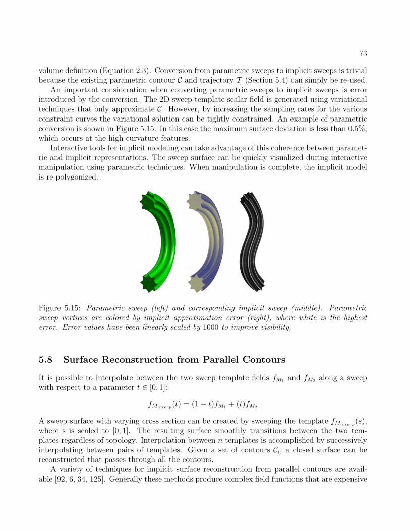
73

volume definition (Equation 2.3). Conversion from parametric sweeps to implicit sweeps is trivialbecause the existing parametric contour C and trajectory T (Section 5.4) can simply be re-used.

An important consideration when converting parametric sweeps to implicit sweeps is errorintroduced by the conversion. The 2D sweep template scalar field is generated using variationaltechniques that only approximate C. However, by increasing the sampling rates for the variousconstraint curves the variational solution can be tightly constrained. An example of parametricconversion is shown in Figure 5.15. In this case the maximum surface deviation is less than 0.5%,which occurs at the high-curvature features.

Interactive tools for implicit modeling can take advantage of this coherence between paramet-ric and implicit representations. The sweep surface can be quickly visualized during interactivemanipulation using parametric techniques. When manipulation is complete, the implicit modelis re-polygonized.

Figure 5.15: Parametric sweep (left) and corresponding implicit sweep (middle). Parametricsweep vertices are colored by implicit approximation error (right), where white is the highesterror. Error values have been linearly scaled by 1000 to improve visibility.

5.8 Surface Reconstruction from Parallel Contours

It is possible to interpolate between the two sweep template fields fM1and fM2

along a sweepwith respect to a parameter t ∈ [0, 1]:

fMinterp(t) = (1 − t)fM1

+ (t)fM2

A sweep surface with varying cross section can be created by sweeping the template fMinterp(s),

where s is scaled to [0, 1]. The resulting surface smoothly transitions between the two tem-plates regardless of topology. Interpolation between n templates is accomplished by successivelyinterpolating between pairs of templates. Given a set of contours Ci, a closed surface can bereconstructed that passes through all the contours.

A variety of techniques for implicit surface reconstruction from parallel contours are avail-able [92, 6, 34, 125]. Generally these methods produce complex field functions that are expensive

74

to evaluate. One benefit of the approach described above is that it is very efficient to evaluate,particularly when the sweep templates are approximated with discrete versions (Section 5.6).In Figure 5.16 a human L3 vertebra is reconstructed from 93 segmented CT slices. It takesapproximately 6 minutes to create the set of high-resolution parallel sweep templates, howeveronce complete the implicit object (which is simply a linear sweep) can be interactively editedusing the system described in Chapter 6 (Figure 5.16c).

Figure 5.16: Surface reconstruction from contours. Human L3 vertebra is reconstructed from 93slices (a,b) and interactively modified in a BlobTree modeling system (c). The high-frequencyridges on the vertebra surface in (b) are due to manual segmentation errors.

5.9 Chapter Summary

A technique has been described for generating 3D implicit sweep volumes that are compatiblewith the BlobTree hierarchical modeling system. The main contribution is the development ofa method for converting a 2D sweep template contour C (or set of contours, including “holes”)into a bounded, continuous 2D scalar field which is used as an implicit sweep template. First,boundary constraints were added to existing variational curve approximation techniques, resultingin a C2 distance field approximation with low normalization error. A constructive field-blendingapproach was used to preserve sharp features in the sweep template. The approach to sweepingthe 2D sweep template field largely follows existing methods, although the integration of variousendcap styles into the implicit sweep formulation is a necessary detail that has not been previouslydescribed.

A key benefit of the sweep volumes described in this chapter is compatibility with BlobTreehierarchical implicit modeling. Existing implicit sweeps either lacked direct profile manipulation,or did not have BlobTree-compatible scalar field properties. The sweep formulation presentedhere combines the desirable attributes of these previous approaches. Particularly in an interactivecontext, these new sweeps provides an expressive, intuitive free-form primitive for the BlobTree.Complex shapes such as the set of pipes in Figure 5.17 can be quickly created by blendingmultiple sweep surfaces. More examples are shown in Chapter 7.

75

Figure 5.17: An intake manifold modeled with Bezier curve sweeps.

Chapter 6

ShapeShop: A Proof-of-Concept

Existing interactive implicit modeling systems are reviewed. A new interactive BlobTree modelingsystem, known as ShapeShop, is introduced. Various aspects of the interface are reviewed, witha particular focus on sketch-based operations. Novel implementation challenges are discussed,followed by suggestions for future work.

Some material in this chapter is taken from the publication “ShapeShop: Sketch-Based SolidModeling with BlobTrees” by Schmidt, Wyvill, Sousa, and Jorge [99]. The material appearinghere is due to Schmidt.

6.1 Interactive Implicit Modeling Systems

Interactive implicit-surface modeling has been a long sought-after goal in computer graphics. Avariety of systems described in the literature have claimed success, however the interpretation ofthe term “interactive” varies considerably. For example, a variety of hierarchical implicit surfacemodeling environments have been developed, notable examples include the various incarnationsof the BlobTree Modeling System [51] and the HyperFun system [4]. In the latter system, claimsof “interactivity” mean only that the underlying skeleton can be manipulated interactively -the surface is not visualized in real-time. Similarly, the convolution-surface modeling systemdescribed by Sherstyuk [106] supports interactive editing of the convolution skeleton, and providescompelling results, however the implicit surface was rendered off-line using ray-tracing.

An early implicit modeling system which did support interactive visualization was reportedby Desbrun [42], where interactivity was achieved by creating a separate polygonization for eachprimitive in the model. This approach is essentially a local-update scheme, closely related to [5]and sharing the same limitation; namely, that if the update region is complex then interactivityfails. To reduce overall computation, level-of-detail (LOD) implicit surfaces were explored byBarbier et al [15]. This technique, first proposed by Bloomenthal and Wyvill [29], uses lower-resolution versions of primitives to speed visualization time. Per-primitive polygonization andlevel-of-detail were combined to rapidly visualize implicit surfaces based on skeletal subdivisioncurves [58]. However, this method was limited to surfaces which can be described by a skeletoncomposed of branching curves. In a similar vein, Akleman [7] employed ray-quadric surfaceswhich supported interactive polygonization but were limited to star-shaped volumes.

Witkin and Heckbert [117] proposed a general technique for interactive implicit surface visu-alization based on “floater” particles, and applied it in an accompanying 3D modeling system.This approach was extended by Hart [56], however that system was limited to constructingsurfaces which could be defined by a single multi-dimensional polynomial. In both cases, onlyrelatively simple models could be constructed.

Variational implicit surfaces (Section 3.5.1) were initially proposed as a method for interactive

76

77

implicit surface modeling [113, 114]. Recent sketch-based modeling systems have adapted thismethod [65, 13]. However, the computational cost of solving for the variational solution limitsthis approach to relatively simple models. A similar issue limits the sketching system describedby Alexe et al [10], which is based on blending large numbers of implicit point primitives.

Distance fields were combined with mesh subdivision techniques in the Skin system [68].While very smooth results were produced, and the technique is quite interactive [59], it does notaddress the problems encountered with real-time visualization of general implicit surfaces.

Much more promising results have been produced by systems which employ implicit surfacesbased on discrete volume datasets. The sculpting system described by Ferley et al [45] is highlyinteractive and supports adaptive volume resolution [46]. Adaptive distance fields have also beenemployed in an interactive volume sculpting system [83]. Owada et al [78] describe a sketch-based modeling system for volumetric data. Volume datasets can be interactively deformedand manipulated using level set techniques [73], and interactively functionally composed [18].However, as noted by [18], hierarchical techniques cannot easily be applied to volume datasetsdue to the massive amount of sample data which must be stored and manipulated.

Several conclusions can be drawn from the review above. First, no existing system sup-ports interactive manipulation and editing of complex hierarchical implicit models. Many ofthe systems described above support some aspects of hierarchical functional implicit modeling,but the general framework is not exploited. Second, systems based on implicits generated fromvolume data have generally supported higher levels of interactivity and more complex models.Attempts to create a synthesis of these two methods lead directly to the hierachical spatialcaching technique described in Chapter 4. In the following sections a novel interactive hierar-chical implicit modeling system is described which, rather then exploiting specific properties ofthe various primitives and operators, relies on this new caching technique to produce interactivevisualization.

6.2 Overview

The ShapeShop hierarchical implicit modeling system began development as a testbed for eval-uating hierarchical spatial caching (Chapter 4). The initial system consisted of a few basicBlobTree primitives and operators [120] which could be created and interactively manipulated ina traditional CAD-style interface. The BlobTree model was visualized using a basic polygoniza-tion algorithm [26], the surface was fully re-polygonized when changes were made to the model.

The CAD-style interface, while functional, was cumbersome and tedious to use. This wasnot entirely due to the actual modeling interface, however. Constructive modeling with thebasic BlobTree primitives (sphere, cylinder, etc [120]) requires many primitives and operators tocreate complex shapes. Creating and placing all these elements is a time-consuming process. Toreduce construction time, the free-form sweep primitives described in Chapter 5 were added tothe system, allowing complex shapes to be created using far fewer primitives. However, instead ofcreating sweep primitives by interactively manipulating parametric curves, a novel sketch-basedconstruction method was implemented [99]. This modification had a significant impact on howmodels were constructed. In particular, “blobby sweep” primitives (Section 5.4.1) have proven

78

to be an incredibly powerful modeling tool.ShapeShop has evolved into primarily a sketch-based BlobTree modeling tool, with elements

of the CAD-style interface still used where sketch-based equivalents have not been developedor implemented. The full CAD-style interface is still available, however the current system isdesigned to be used for sketch-based model construction. In the following sections, the non-standard elements of the ShapeShop modeling system will be described, followed by details onthe internal architecture of the BlobTree implementation.

6.3 ShapeShop Interface

A screenshot of the ShapeShop user interface is shown in Figure 6.1. The system is implementedon Microsoft Windows using the MFC C++ application framework. The main interface windowis the single-pane model view. Two additional windows are used to manipulate the scene - a treeview for interacting with the current BlobTree hierarchy, and a list view for changing parametersof a single tree node. Standard menus and toolbars are also used to control functionality whichhas not yet been implemented in the sketch-based interface.

Various sketch-based interface components are embedded in a Heads-Up Display (HUD) ren-dered over top of the model view. The Expectation List dynamically responds to sketches drawnby the user, offering possible model interactions. The Parameter Toolbar offers interactive ma-nipulation of the most commonly-used parameters of the selected node. Similarly, the OptionsToolbar provides access to frequently changed scene parameters, and the View Toolbar providesinteractive camera control.

6.4 Sketch-Based Modeling Operations

In contrast to traditional 3D modeling interfaces, which are generally based on manipulationof control points and abstract parameters, Sketch-Based Modeling systems attempt to explicitlyinfer 3D shape from hand-drawn strokes. A variety of approaches have been taken. Systemssuch as SKETCH [126] and GiDES++ [63] generate polyhedral objects based on simple gestures.In the Teddy [60, 59] system, arbitrary strokes were used to directly specify free-form modelingoperations. A variety of recent works [65, 13, 78, 112, 36, 10] have explored this style of interface.Most of these systems have been based on volumetric implicit surface shape representations,however none of these systems take advantage of hierarchical implicit modeling.

ShapeShop largely follows the free-form sketch-based modeling interface style introducedby [60]. The primary shape-creation operation in these interfaces is inflation, where a closed 2Dcontour is inflated into a “blobby” 3D shape. This operation can be easily accomplished usingimplicit sweeps with the “blobby” endcap style, as described in Section 5.4.1. The 2D sketch(Figure 6.2a) is projected onto a plane through the origin parallel to the current view plane,and then inflated in both directions (Figure 6.2b). After creation, the width of the primitivecan be manipulated interactively with a slider (Figure 6.2c). The inflation width is functionallydefined and could be manipulated to provide a larger difference between thick and thin sections.One advantage of an implicit representation is that holes and disjoint pieces can be handled

79

Figure 6.1: ShapeShop user interface screenshot. The various major interface elements includethe (A) Parameter Editor, (B) BlobTree Editor, (C) Expectation List, (D) Parameter Toolbar,(E) Options Toolbar, (F) View Toolbar, and (G) Model View.

80

transparently.

Figure 6.2: Blobby inflation converts the 2D sketch shown in (a) into the 3D surface (b) suchthat the 2D sketch lies on the 3D silhouette. The width of the inflated surface can be manipulatedinteractively, shown in (c). Sketched 2D curves can also be used to create (d) linear sweeps and(e) surfaces of revolution.

The sweep surface representation underlying this blobby inflation scheme also supports linearsweeps (Figure 6.2d) and surfaces of revolution (Figure 6.2e). Linear sweeps are created in thesame way as blobby shapes, with the sweep axis perpendicular to the view-parallel plane. Theinitial length of the sweep is proportional to the screen area covered by the bounding box of the2D curve, but can be interactively manipulated with a slider. Surfaces of revolution are createdby revolving the sketch around an axis lying in the view-parallel plane. Revolutions with bothspherical and toroidal topology can be created.

Existing sketch-based systems have generally not included these additional types of shapes1

While blobby inflation is highly useful for many modeling tasks, linear sweeps and revolutionsare invaluable in situations such as mechanical modeling. In particular, surfaces of revolutionare a class of shape that cannot be approximated with blobby inflation.

Since the underlying shape representation is a true volume model, cutting operations can beeasily implemented using CSG operators. Users can either cut a hole through the object or removevolume by cutting across the object silhouette. Once a hole is created the user may transformthe hole interactively. An interactive control is also available to modify the depth of cuttingoperations. Cut regions are represented internally as linear sweeps, no additional implementationis necessary to support cutting in the BlobTree. An example is shown in Figure 6.3. This CSG-based cutting operation is both more precise and less restrictive than in existing systems.

To create more complex free-form shapes, the user can blend new blobby primitives to thecurrent volume via oversketching. To position the new blobby primitive, rays through the sketchvertices are intersected with the current implicit volume. The new primitive is centered atthe average z-depth of the intersection points. The width of the new blobby primitive can bemanipulated with a slider, as can the amount of blending. Blended volumes can be transformedinteractively, an example is shown in Figure 6.4. Karpenko et al [65] supported sketching of theblend profile but also noted that this technique was not robust and is very slow to compute. Thelevel of control over the blend surface provided in ShapeShop has not been available in previoussketching systems.

Any BlobTree primitive can be used to add surface detail based on sketches. As an initialexperiment, ShapeShop supports “surface-drawing”. Rays through the 2D sketch are intersected

1A notable exception is the more advanced revolution technique of Cherlin et al [36]

81

Figure 6.3: Cutting can be performed (b) across the object silhoutte or (c) through the objectinterior. Holes can be interactively translated and rotated. Intersection with other holes is auto-matically handled, as shown in (d). Hole depth can also be interactively modified to create cut-outregions (e).

Figure 6.4: The sketch-based blending operation (a) creates a new blobby inflation primitive(b) and blends it to the current volume. The blending strength is parameterized and can beinteractively manipulated, the extreme settings are shown in (c) and (d). The blend region isrecomputed automatically when the blended primitives move, as shown in (e).

with the current implicit volume, and a 3D implicit polyline primitive is generated. Interactivecontrols are provided to manipulate both the surface radius and linear scaling (tapering) alongthe polyline. Results are shown in Figure 6.5.

Surface drawing with implicit volumes is a very flexible technique. Any pair of implicitprimitive and composition operator can be used as a type of “brush” to add detail to the cur-rent surface. For example, creases could be created by subtracting swept cone primitives usingCSG operations. Implementing these alternative tools within the BlobTree framework is verystraightforward. In addition, since each surface-drawing stroke is represented independently inthe model hierarchy, individual surface details can be modifed or removed using the existingmodeling interface.

By surface-drawing on temporary construction surfaces, it is possible to create non-planar3D geometry that would otherwise be impossible to sketch (Figure 6.5d,e). These temporaryconstruction surfaces are a novel property of ShapeShop which was not designed into the system,but simply emerged out of the non-linear hierarchical editing capabilities of the BlobTree.

82

Figure 6.5: Surface-drawing is specified by a 2D sketch, as shown in (a). Blended skeletal implicitpoint primitives are placed along the line at intersection points with the model, shown in (b). In(c) the radius of the points is increased and then tapered along the length of the 2D curve.Temporary construction surfaces (d) can be used to create more complex 3D curves (e).

6.5 Node Selection and BlobTree Traversal

Procedurally-defined BlobTree volumes inherently support non-linear editing of internal treenodes. However, before a primitive can be manipulated it must be selected. One option isto cast a ray into the set of primitives and select the first-hit primitive. This technique isproblematic when dealing with blending surfaces, since the user may click on the visible surfacebut no underlying primitive is hit.

Picking in ShapeShop is implemented by intersecting a ray with the current volume, and thenselecting the primitive which contributes most to the total field value at the intersection point.This algorithm selects the largest contributor in blending situations, and selects the subtractedprimitive when the user clicks on the inside of a hole surface created by CSG difference operations.However, selecting the largest field-value contributor can result in un-intuitive behavior in caseswhere a small primitive is blended with a larger one, as the larger primitive may contribute moreto the field at all points on the surface. In this case, the user must use the BlobTree Editor treeview (Figure 6.1) to select the desired node.

This selection system only allows for selection of primitives. To move up the tree to parentnodes, a parent gesture is implemented which selects the parent of the current node. The parentgesture is entered as a straight line towards the top of the screen. No similar child gesture hasbeen implemented because it is unclear how to disambiguate which child is desired in cases wherea node has multiple children. More complex tree traversal and manipulation, such as re-arrangingnodes, currently requires the use of the BlobTree Editor tree view.

A selected primitive or composition node can be removed using a simple erase gesture, enteredas a small “scribble” over top of the selected primitive. Removing a compostion node is equivalentto cutting a branch from the model tree - all children are also removed.

6.6 BlobTree Visualization

To interactively visualize BlobTree models in ShapeShop, real-time polygonization of the surfaceis performed. The system supports a variety of algorithms, the most basic being an optimizedversion of Bloomenthal’s polygonizer [26]. Two modified versions of this polygonizer are alsoavailable. The first simply adds the crease-finding techniques described in the Extended Marching

83

Cubes work [66]. The second provides support for local updates, where re-meshing is limited tothe regions in which the current model has changed.

Note that supporting partial re-meshing introduces significant complexity - the polygonizermust maintain knowledge about which triangles and vertices are associated with each polygoniza-tion cube, and the mesh must support efficient partial decimation. The overhead from theseoperations is significant, in particular when re-meshing the entire surface the local update poly-gonizer takes approximately twice as long as the standard polygonizer. However, since smallerlocal updates are so much more efficient, the benefits largely outweigh this particular cost.

All the polyognization algorithms used in ShapeShop are descendants of the method in-troduced by Wyvill et al [124] which is commonly referred to as marching cubes [67]. Thesealgorithms are known to produce meshes with many near-degenerate triangles. To improve meshquality, Ohtake’s mesh refinement algorithm [76] has been implemented. The user can choose toalways apply this algorithm as a meshing post-process, however it is expensive and can greatlyreduce interactivity. As an alternative, a “Quick Refine” button is available which runs 5 it-erations of mesh relaxation. This significantly improves triangle quality and only takes a fewseconds for moderately complex models.

When a primitive or sub-tree of the model hiearchy is selected, it is often non-obvious whatthe shape of the selected internal volume is (particularly in blending situations). To assist incomprehension, several rendering modes have been implemented to display the selected volume(Figure 6.6). Another option is to visualize the influence region of a volume by coloring the meshbased on the field value of the selection.

Figure 6.6: Internal volumes can be directly rendered using (a) transparency, (b) silhouette lines,or (c) transparency and silhouttes. Mesh highlighting can also be used to convey the influenceregion of a selection, as in (d) and (e).

6.7 BlobTree Implementation Details

The BlobTree [120] implementation used in ShapeShop is relatively non-traditional, comparedto recent implementations such as that described by [51]. First, only portions of the BlobTreerelating specifically to shape modeling have been implemented. Additional functionality, suchas color, texture, and animation have been avoided to simplify the implementation and reducecomputational costs. Some of these exclusions have been driven by the use of Hierarchical SpatialCaching (Chapter 4) - for example, adding floating-point RGBA color caches would quadruplethe memory requirements (and update time) for each cache.

84

Another significant difference is in the division of BlobTree functionality. ShapeShop usesa 3-tiered object-oriented BlobTree architecture. The lowest tier is a library of basic implicitsurface objects, including various primitives and composition functions. All objects implement ageneric ScalarField interface which defines basic functions for computing the field value, gradient,bounding box, and seed points. None of the objects at this level have any notion of a hierarchicalorganization.

The second tier represents the standard BlobTree hierarchical modeling system. A varietyof primitive and operator nodes are implemented, some which simply wrap objects from theimplicit surface library, and others which are an aggregation of multiple implicit surface objects.All composition nodes at this level have an associated spatial cache, following the tightly-coupledcaching implementation style described in Section 4.5. Similarly, all nodes support a basic event-passing mechanism for notifying parent nodes about invalidation events.

The third tier can be considered the user-interface view of a BlobTree. The nodes at thislevel largely wrap nodes at the BlobTree level, adding functionality for supporting the varioususer-interface tools and parameter editors. However, nodes at this level can also represent anaggregation of multiple BlobTree nodes, providing a conceptual overview of an otherwise muchmore complicated underlying structure.

While this three-tiered architecture may seem over-engineered, the benefits have alreadybeen hinted at above. By separating implicit surface functionality from the BlobTree nodes,more complex BlobTree nodes can easily be assembled. Since all implicit surface objects supportthe same basic interface, alternate implementations can be quickly swapped in and out withoutsignificant changes to the BlobTree code. Similarly, changes to the user-interface do not requiremodification of the BlobTree or implicit surface packages. The ability to present a “conceptual”BlobTree to the user which does not actually map one-to-one to the actual BlobTree nodes is alsodesirable from a user-interface perspective. For example, the model tree view can be simplified bynot explicitly representing transformation nodes, reducing apparent tree complexity and depth.

The notion of a “conceptual” BlobTree also provides an avenue for transparently supportingdynamic BlobTree optimization. A variety of techniques for dynamically re-organizing a BlobTreeto provide more efficient evaluation have been developed [15]). However, it is not appropriateto present this optimized tree directly to the user. In most cases, the model tree will have beencarefully arranged to preserve certain abstract hierarchical divisions. While perhaps less efficient,the user-defined organization must be preserved. The user-interface tree can easily provide thisview, while the underlying BlobTree can be freely optimized. While these techniques have yetto be implemented in ShapeShop, they will not require any significant architectural changes tosupport.

6.8 Limitations and Future Work

ShapeShop is, at this time, only a proof-of-concept system. Interactive hierarchical implicitmodeling is a relatively unexplored area, largely because real-time interaction was very limitedprior to the development of hierarchical spatial caching. Experience with the ShapeShop interfacehas raised a variety of issues, some well-known, and others less obvious.

85

A key limitation exists in ShapeShop regarding visualization of sharp creases and other high-frequency features on complex models. Adaptive polygonization schemes [53, 5, 14] may signifi-cantly improve visualization of small features. However, as shown in Section 4.8.4, hierarchicalspatial caching interferes with existing techniques for improving crease reconstruction. Adaptivepolygonization will not improve this situation, new techniques must be developed.

In the user interface, one of the biggest challenges is interacting with the BlobTree hierarchy.The parent gesture described in Section 6.5 only allows the user to traverse the tree in an upwarddirection. Download traversal, or selection of non-leaf nodes, must occur through the BlobTreeEditor tree view 6.1. However, for deep or large trees, this tree view quickly becomes extremelydifficult and time-consuming to use. A better solution for tree traversal is needed, preferablyone which can be applied directly in the model view, without the aid of a separate tree view. Afurther problem is how to support tree manipulation directly in the model view.

Closely related to tree traversal is the problem of visualizing internal nodes and sub-trees ofthe BlobTree model. The techniques for mesh highlighting and internal visualization described inSection 6.6 are ad-hoc methods that were simply easy to implement. User studies are necessaryto determine which techniques are most effective at conveying both node shapes and the BlobTreestructure.

A final problem, which concerns any functional implicit modeling system, is that of repro-ducibility. Many of the primitives and operators used in ShapeShop are highly complex andcannot be described with a simple functional definition. For example, the variational-curve-based sweep primitives of Chapter 5 rely not only on many parameters, but on a variety of otheralgorithms. Unless these algorithms are duplicated exactly, the resulting scalar fields will bedifferent. Hence, transferring models from ShapeShop to future implicit modeling systems (oreven future versions of ShapeShop) may not produce the same results. There is no easy solutionto this problem. One approach may be to re-write the implicit surface library using some virtualmachine language, and package the implicit library with each saved file. A similar method is usedby the HyperFun [4] system, although the use of interpreted code there is unlikely to provideinteractive performance.

6.9 Chapter Summary

Interactive tools for hierarchical implicit modeling systems such as the BlobTree have tradi-tionally been very limited. Systems for real-time manipulation of skeletal primitives have beendeveloped, but interactive visual feedback on the changing implicit surface did not scale beyondtrivial models. The ShapeShop system presented in this chapter is essentially the first systemto provide scalable interactive visualization of complex BlobTree models as they are modified.ShapeShop has a novel sketch-based interface which supports fast and intuitive constructionof complex models. A variety of other technical issues relating to interactive BlobTree editinghave also been discussed, such as direct selection of primitives and dynamic highlighting of se-lected regions. Various issues relating to the implementation of BlobTree data structures usedin ShapeShop were covered, and directions for future work were suggested.

Chapter 7

Results and Conclusion

A task-based analysis of the ShapeShop interactive BlobTree modeling system is performed byconsidering a series of possible applications. Directions for future work are considered, followedby a summary of the thesis.

Some images in this chapter are taken from the publications “Interactive Implicit Modeling withHierarchical Spatial Caching” by Schmidt, Wyvill, and Galin[97], “Generalized Sweep Templatesfor Implicit Modeling” by Schmidt and Wyvill [96], “Sketch-Based Modeling with the BlobTree”by Schmidt, Wyvill, and Sousa[98], “ShapeShop: Sketch-Based Solid Modeling with BlobTrees” bySchmidt, Wyvill, Sousa, and Jorge [99], “Sketch Based Construction and Rendering of ImplicitModels” by Wyvill, Foster, Jepp, Schmidt, Sousa, and Jorge [119], “Interactive Decal Com-positing with Discrete Exponential Maps” by Schmidt, Grimm, and Wyvill [94], and “InteractivePen-and-Ink Rendering for Implicit Surfaces” by Schmidt, Isenberg, and Wyvill [95]. The imagesappearing here are due to Schmidt.

7.1 Results

The goal of this thesis, as stated in section 1.4, is to provide a framework in which interfaces forinteractive hierarchical implicit modeling can be explored. In some sense, determining whether ornot this goal has been met is trivial. An implicit modeling system has been created. ShapeShopenables interactive BlobTree modeling in a way that was not previously possible. The technicalmerits of Hierachical Spatial Caching and implicit sweep surfaces were demonstrated in theirrespective Chapters (4 and 5).

However, these technical evaluations have only moderate relevance to the actual interac-tive experience. The important question is whether or not implicit modeling in ShapeShop isuseful. Of course, as research software, ShapeShop cannot be reasonably compared to well-established commercial products. Standard interface evaluation methods are also difficult toapply. ShapeShop’s underlying implicit shape representation is radically different from tradi-tional modeling interfaces, as is the sketch-based interface. Under these conditions, isolatingrelevant factors which can be subjected to HCI evaluation techniques provides little informationabout the system as a whole. Furthermore, many aspects of the user interface have been givenonly limited attention, so test subjects are likely to encounter problems which are completelyunrelated to implicit modeling.

How, then, can ShapeShop be evaluated? The approach taken in this chapter is to demon-strate the effectiveness of ShapeShop at supporting a variety of modeling tasks. Unfortunatelythe format of this thesis has limited capability for demonstrating interactive tasks. As a conso-lation, several 3D models have been produced for each task. In some cases, the models are quickexamples, while others are the result of many hours of effort and test the limits of ShapeShop.

86

87

The intent is to convey some sense of what ShapeShop is good at, and the potential of interactivehierarchical implicit modeling.

7.1.1 Interactive Assembly

One very basic task in shape modeling is assembling a complex model from a set of simplercomponents. Compared to implicit surfaces, B-Rep modeling systems have limited support forthis task. Part assembly is common in CAD systems, however generally the parts are simplypositioned, rather than combined. Mesh and spline modeling tools rarely provide any facility forcomposing complex shapes. However, this task is generally not interactive for implicit models -times are often reported in minutes for complex models [11].

As discussed in Section 4.8, ShapeShop supports interactive assembly of relatively compleximplicit models. The timings there showed that blended components of the Medusa model, madefrom 9490 skeletal point primitives segmented into 7 parts, could be manipulated at several framesper second. Various parts of the Medusa model have also been combined with other compleximplicit models, as shown in Figure 7.1. Note that the mesh resolutions shown in these figuresare significantly higher than those used during interaction. However, interactive mesh resolutionswere sufficient to carry out position fine-tuning without extensive checking at higher resolutions.

Figure 7.1: Interactive assembly of complex implicit models. An initial design study of combiningthe Medusa model of Chapter 4 with an implicit cup (left), and the final result rendered with avolume texture (center). Letters were added to the tail using surface drawing (Section 6.4). TheMedusa head was also combined with an implicit cup (right).

Another model created from interactive assembly is shown in Figure 7.2. In this case, theindividual components (arm, leg, body, head, and wing) were created in ShapeShop, using thesketch-based interface. These parts were then imported and assembled into a final model con-taining 65 linear sweep primitives and 35 composition operators.

88

Figure 7.2: A complex implicit Gremlin model (left). A simplified version (middle) has beentextured using a decaling technique [94] (right).

7.1.2 Character Modeling

While this research has focused on the shape modeling properties of hierarchical implicit surfaces,another key benefit is that the model hierarchy can be trivially animated [120]. Combined withsmooth blending, BlobTree models are a powerful tool for representing both the shape and motionof animated characters.

Some character models created with an early version of ShapeShop are shown in Figure 7.3.These models are notable because although the interactive tools available at the time were verylimited, each of these models was generated in a single session lasting under an hour (a necessity,since the software did not then support saving or loading). The models shown are also the initialattempts at each character. ShapeShop easily supports this style of free-form, experimentalmodeling, and generally produces meaningful results.

Likewise, the skeleton model in Figure 7.4 was sketched in a single session, this time on thesecond try (the system crashed half-way through the first trial). The model is fully articulatedand could easily be animated. A notable feature of this model is the skull, which was initiallycreated as a solid volume. Later in the session, the interior was removed using CSG subtractionoperations, and exposed by cutting out the eyes and nose. These changes took only a few minutes.Performing similar modifications on most B-Rep models would require significantly more usereffort.

A common workflow for character modeling is to first create a clay sculpture of the characteras a design study, and use it as a basis for the 3D computer model. An attempt was made tomimic this process using the clay statue in Figure 7.5. Note that this model would be difficultto laser scan, due to the complex topology. In terms of exact duplication, the test was clearlynot a success. However, very little time was spent refining the model. The goal was to createa quick approximation that could be used as a basis for texture mapping. ShapeShop met thisobjective; the modeling time was under half an hour. One of the reasons clay modeling is still

89

Figure 7.3: Early examples of character models sketched using ShapeShop. The rat (left) andscorpion (right) were created entirely using sketched blobby primitives. The elephant (center) isa combination of standard implicit primitives, sketched primitives, and a bezier sweep for thenose.

Figure 7.4: A skeleton model sketched in ShapeShop. The head of the skull has been hollowed outusing CSG operations, and the bones are articulated such that they can be animated directly.

90

performed is that clay is more malleable than the computer representation and easily supportsglobal modification. Implicit modeling, which easily supports large-scale manipulation of blendedsurfaces, may have some impact on this practice.

Figure 7.5: An elephant model (middle) sketched based on an existing physical clay elephantstatue (left). Sketching this model took under half an hour. Additional surface detail was addedusing texture mapping (right).

Finally, a re-posing task similar to that which would be carried out in character animation isshown in Figure 7.6. ShapeShop’s interface does not fully support hierarchical re-posing, so themodifications shown are rather slight. However, these two poses could easily be interpolated tocreate a short animation.

Figure 7.6: A dog model sketched using ShapeShop. The hierarchical organization of the modelcorresponds to the anatomical organization, allowing the figure to be easily re-posed.

7.1.3 Mechanical Parts

Computer-Aided Design (CAD) is perhaps the most common application of 3D modeling. Theuse of computer modeling in product engineering has become almost ubiquitous. Solid models areused in design, manufacturing, and engineering analysis. The guaranteed validity and analyticproperties of implicit surfaces have clear benefits here. A variety of basic models of physical

91

objects are shown in Figure 7.7. The piston model in that figure demonstrates a one of the novelcapablities of ShapeShop. This model has multiple interior holes but was sketched in under 10minutes (and done with a mouse, instead of a tablet). The goal here was not to create a partready for production, but rather to demonstrate that ShapeShop can be used as an effectivetool to convey an idea. To work at this speed, product designers are generally limited to 2Dsketching, which is very flexible but has limits when used for representing 3D shapes.

Figure 7.7: Mechanical objects. The piston on the left was sketched in under 10 minutes, despiteit’s complex topology.

Another engineering model is shown in Figure 7.8. This car model was initially constructedin much the same way as the physical clay prototypes used by the automotive industry - as asolid block. The interior was then hollowed out, and seats and windows were added. The easewith which this process was carried out suggests an alternate workflow for car modeling. Claybody prototypes are already routinely laser scanned. The results could easily be converted toimplicit form using any of the techniques mentioned in Section 3.5, and the interior interactivelymodeled using ShapeShop. It has already been noted that composing implicit surfaces is trivial,so part libraries could be easily integrated.

Figure 7.8: Car model sketched using ShapeShop. The interior structure was added after theinitial car body was designed. A cut-away view is shown on the right.

A third model is shown in Figure 7.9. Taking a more traditional CAD approach, this model iscreated entirely out of sweep primitives. However, implicit blending is used to create water-tightsmooth joints between surfaces. Since the model is actually an implicit volume, it can be useddirectly to generate surface and volume meshes suitable for use in physical simulations.

92

Figure 7.9: Shuttle model created using implicit sweep primitives. Sweep primitives can be blendedwith arbitrary levels of smoothness.

7.1.4 Biological Modeling

One of the widely-recognized benefits of implicit surfaces is their ability to represent the smooth,amorphous surfaces often found in nature. Recent interest in surgical simulators and large-scalesimulation of human biology have increased the need for physiological models. The possibilityfor interactive manipulation of shapes reconstructed from CT data was already examined inSection 5.8. Another option is shown in Figure 7.10, where a 3D model of a human heart hasbeen sketched. Modeling time was approximately 30 minutes. The heart is not biologicallyaccurate, but clearly demonstrates the ability of ShapeShop to represent the smooth, complexbranching structures found in nature. Smaller features such as veins, which may be difficult toreconstruct from scan data, can be easily added. The use of such quickly-sketched biologicalmodels for use in medical training has been previously examined [14].

Figure 7.10: Heart model sketched using ShapeShop in approximately 30 minutes. Complexinterlocking branching structures can easily be created by concatenating smaller segments.

93

7.1.5 Design Iteration

A significant portion of most design cycles is iteration. Computer modeling easis this process, ascomputer models are generally cheaper than their physical counterparts. However, with B-Repsystems it is still often necessary to “start from scratch” if significant changes are necessary. Thenon-linear editing capabilities of the BlobTree can minimize the need to re-start, or at least allowsatisfactory portions of the previous iteration to be easily cannibalized. Several design iterationswere performed on the basic dog model shown in the left of Figure 7.11. A notable modificationis the addition of the pig nose in the rightmost model. The pig nose was simply sketched overtop of the existing dog nose, and blended with the model. In a B-Rep system, this would likelyhave produced an invalid model. Blending composition in the BlobTree simply combines theunderlying functions, resulting in a well-defined volume.

Figure 7.11: Design iterations on a basic dog model (left). The implicit model can be easilymodified by deleting components and sketching new ones. The pig nose (right) was simply blendedonto the existing model.

7.1.6 Observations

The models shown in the previous sections clearly demonstrate both the benefits and limitationsof ShapeShop. In it’s current form, ShapeShop is usable primarily as a rapid prototyping toolfor 3D models. This is in some part decided a priori by the sketch-based interface, whichemphasizes speed over precision. However, various limitations in both the interface and thecurrent implementation prevent ShapeShop from scaling to very complex models. To give somesense of the limits of ShapeShop, the full Gremlin model in Figure 7.2 can only be manipulatedinteractively if the mesh resolution is very low, too low to be really considered usable. However,initial experiments with adaptive polygonization indicate that this is only a temporary limitation.

Whether for use as an exploratory design environment, teaching aid, or virtual back-of-a-napkin, ShapeShop provides a compelling 3D modeling experience. As the 3D doodle belowdemonstrates, ShapeShop enables a style of 3D modeling that is non-existent in current B-Rep-based tools.

7.2 Future Work

The ideas presented in this thesis suggest various directions for future work. In terms of thetheory of implicit surfaces, the classification produced in Chapter 3 should be analyzed further,

94

Figure 7.12: A 3D Doodle

and likely refined. There is a bias towards solid modeling in the properties selected to organizeand compare the different techniques. An application-independent approach may be beneficial.Further analysis of normalization properties would be particularly useful, as normalization errorhas a significant impact on many algorithms.

Hierarchical Spatial Caching has proved to be quite successful at increasing visualizationspeed in ShapeShop. However, a variety of limitations exist in the current implementation. Theloss of sharp features is a significant drawback which should be addressed. Separable operators(Section 4.5) may produce significant speed-ups, and should be explored, as should automatedcache management algorithms based on more detailed scene analysis. Another significant im-provement would be the development of adaptive-sampling methods that preserve higher-orderfield continuity.

The implicit sweep surfaces developed in Chapter 5 can be improved in a variety of ways.Boundary constraints in the sweep template are currently placed in somewhat of an ad-hocmethod. Level-set interfaces propagating at curvature-dependent speed could be used to generatemore controllable boundary constraints. The 2D distance field approximation technique couldalso be extended to 3D, although the computational cost of solving the dense variational systemwill be challenging to overcome. In terms of the 3D sweeps, one limitation is that numericalroot-finding is usually necessary in the case of curved trajectories. Root finding is expensiveand requires an analytic expression for the curve tangent to function robustly. A key avenuefor future work is a more general implicit sweep formulation that does not rely on root-finding.A constructive approach based on approximation by union of linear segments can be employed,however this technique breaks down in regions with high curvature. Approximation by union ofsimpler curved segments could provide superior results.

Finally, ShapeShop enables a wide range of possible future work on interactive BlobTreemodeling. Comparable systems simply do not exist, so research on human factors in interactiveimplicit modeling is essentially an open field. The implementation simplicity of implicit solid

95

modeling makes development of new interaction techniques very straightforward, however caremust be taken to extract what is useful from what is possible. Of particular use would be free-form local and global deformation tools. A variety of other current problems were discussedin Section 6.8. One particularly challenging issue which bears repeating is the reproducibilityproblem, which must be addressed if implicit modeling is to enter the mainstream.

7.3 Conclusion

In Chapter 1, two key limitations that essentially prevent interactive BlobTree modeling wereidentified - interactive visualization and direct surface manipulation. The stated goal of thisthesis was to address these issues, and produce a framework which could be used to exploreinteractive tools for hierarchical implicit modeling. Several contributions have been made inpursuit of this goal.

First, chapters 2 and 3 provided a summary and comparison of current techniques for shapemodeling with implicit surfaces. The novel classification developed there was used to justify thechoice of the BlobTree modeling framework as a suitable basis for an interactive system.

The interactive visualization problem was addressed in Chapter 4, with the introduction ofHierarchical Spatial Caching. This novel technique was shown to provide an order-of-magnitudeimprovement in visualization times for relatively complex hierarchical implicit models. Thisspeed-up is sufficient to enable real-time visual feedback of a changing implicit surface as theunderlying hierarchical model is manipulated. Finally, an extensive evaluation of Adaptive Dis-tance Fields was carried out, resulting in the identification of several issues which prevent theiruse for spatial approximation of smooth scalar fields.

Implicit sweep surfaces which support direct manipulation of the sweep profile were introducedin Chapter 5. To generate these sweep volumes, a novel approach to C2-smooth 2D distance fieldapproximation was developed. A technique for preserving creases in the sweep template waspresented, and three different sweep endcap variations were described. These sweep surfaces arecompatible with the BlobTree, providing a powerful and intuitive new tool for quickly modelingmore complex shapes.

A proof-of-concept interactive BlobTree modeling environment was described in Chapter 6.This system, known as ShapeShop, includes both a traditional CAD-style interface and a novelsketch-based modeling input system. A variety of details on the implementation were discussed,and an informal evaluation of the system was related in Section 7.1.

Interactive visualization and direct surface control are long-standing problems in hierachi-cal implicit modeling. Hierarchical spatial caching makes a considerable advance over existingtechniques. The new sweep surfaces presented in this work give significantly more control overthe implicit surface than is available in previous BlobTree modeling systems. Clearly, neitherof these problems can be considered to be solved. However, no interactive BlobTree modelingsystem comparable to ShapeShop has been published to date, and ShapeShop could not havebeen developed without either of these two new techniques. Hence, the goals of this thesis havebeen met. Further, it is hoped that ShapeShop demonstrates the viability of hierarchical implicitmodeling in interactive design, and will enable future research in this direction.

Appendix A

Linear and Quadratic Reconstruction Filters

A variety of reconstruction filters have been proposed for creating a continuous 3D signal based ona set of uniformly-spaced 3D sample poitns. A variety of techniques are surveyed by Marschnerand Lobb [69]. While the tri-cubic and windowed sinc filters were identified as producing thesmoothest reconstructions, these filters require a large number of samples and are expensive toevaluate. For example, the tri-cubic filter requires 64 field samples and evaluation of 21 cubicpolynomials. These filters are impractical for interactive applications. The tri-linear and tri-cubicfilters described in this appendix provide moderate smoothness at an acceptable cost.

A.1 Tri-Linear Reconstruction Filter

The tri-linear reconstruction filter [69] is a separable, C0 continuous filter. Evaluation of the filterat a point p requires 8 neighbouring samples. The filter is an interpolating filter, passing directlythrough the sample points. The three-dimensional filter is defined in terms of 7 applications ofthe one-dimensional linear reconstruction filter Rl, which is simply a linear interpolation betweenthe sample points si and si+1

Rl (si, si+1, t) = (1 − t)si + t si+1

Rl reconstructs a signal over the interval I = [i, i + 1]. The parameter t ∈ [0, 1] is defined overI.

The tri-linear filter Rl3 is defined in terms of Rl. Evaluating Rl3 at a 3D sample pointp requires 8 neighbouring voxels, with the nearest voxel being referred to as vijk. The one-dimensional parameter t is computed along each grid axis, these are denoted ti, tj, and tk.Rl3(p) is calculated by repeated applications of Rl:

Ri(φ, ρ) = (1 − ti)viφρ + ti v(i+1)φρ

Rj(ρ) = (1 − tj)Ri(j, ρ) + tj Ri(j + 1, ρ)

Rl3(p) = (1 − tk)Rj(k) + tk Rj(k + 1)

Here φ and ρ are placeholders. Ri(φ, ρ) is an evaluation of Rl in the i direction, and Rj(ρ) is anevaluation of Rl in the j direction.

A.2 Tri-Quadratic Reconstruction Filter

The tri-quadratic reconstruction filter [18] is a separable, C1 continuous filter. Evaluation ofthe filter at a point p requires 27 neighbouring samples. The filter is an approximating filterand hence does not necessarily pass through the sample points. The three-dimensional filter is

96

97

defined in terms of 13 applications of the one-dimensional quadratic reconstruction filter, whichwill be described first.

Evaluation of the 1D quadratic B-spline filter Rq requires 3 sample points si−1, si, and si+1

to reconstruct a signal over the interval I = [i − 0.5, i + 0.5]. Rq is a function of one parametert ∈ [0, 1] defined over I.

The 1D quadratic B-spline filter Rq is defined as

Rq (si−1, si, si+1, t) =(

si−1 + si+1

2− si

)t2 + (si − si−1) t +

si−1 + si

2

The tri-quadratic filter Rq3 is defined in terms of Rq. Evaluation of the filter at a 3D samplepoint requires 27 neighbouring voxels. For a 3D sample point p, find the nearest voxel vijk. Theone-dimensional parameter t is computed along each grid axis, these are denoted ti, tj, and tk.Rq3(p) is calculated by repeated applications of Rq, defined in the the following set of equations.

Ri(φ, ρ) = Rq

(v(i−1)φρ, viφρ, v(i+1)φρ, ti

)

Rj(ρ) = Rq (Ri(j − 1, ρ),Ri(j, ρ),Ri(j + 1, ρ), tj)

Rq3(p) = Rq (Rj(k − 1),Rj(k),Rj(k + 1), tk)

Here φ and ρ are placeholders. Ri(φ, ρ) is an evaluation of Rq in the i direction, and Rj(ρ)is an evaluation of Rq in the j direction.

Appendix B

Variational Implicit Curves

A common approach to generating a 2D scalar field is to interpolate a set of 2D field valuesamples (mi, vi), where vi is the desired field value at point mi. One well-known technique isvariational interpolation based on thin-plate splines, which produces a globally C2 field. Thisscattered data interpolation technique has been used define implicit curves and surfaces [113].

The thin-plate spline f(u) is defined in terms of points (mi, vi) weighted by coefficients wi,and a polynomial P(u) = c1ux + c2uy + c3:

f(u) =∑

wi‖u − mi‖2 ln(‖u − mi‖) + P(u) (B.1)

The weights wi and coefficients c1, c2, and c3 are found by solving a linear system definedby evaluating Equation B.1 at each known solution f(mi) = vi. The resulting linear system isa dense matrix with dimension (N + 4)2 . The coefficients determined by solving this systemdescribe a variational solution which is guaranteed to interpolate all sample points (vi, vi) withsecond-derivative continuity while minimizing a global curvature metric [44].

98

Appendix C

Normalized Implicit Polygons

A 2D closed contour C can be represented by an implicit polygon defined using the followingapproach (reproduced from [22]). First, C is approximated with a set of line segments. Then fora segment ((x1, y1), (x2, y2)), with d =

√(x2 − x1)2 + (y2 − y1)2, a scalar field can be defined:

f(x, y) =1

d((x − x1)(y2 − y1) − (y − y1)(x2 − x1)) (C.1)

A circular scalar field is also defined for the line segment:

t(x, y) =1

d

[(d

2

)2

− (x −x1 + x2

2)2 − (y −

y1 + y2

2)2

](C.2)

This circular field is used to normalize the line segment field, defining a new scalar field h:

h =√

f 2 + 0.25 ∗ (|t| − t)2 (C.3)

These normalized line segments are then combined using the R-conjunction operator:

F (h1, h2) = h1 + h2 −√

h21 + h2

2 (C.4)

The resulting field is unsigned, but since C is closed a polygon point-containment test can beused to determine whether a distance value should be positive or negative.

99

Bibliography

[1] Abdel-Malek, K., Blackmore, D., and Joy, K. Swept volumes: Foundations, per-spectives and applications. submitted to International Journal of Shape Modeling (2000).

[2] Abdel-Malek, K., Yang, J., and Blackmore, D. Closed-form swept volume of im-plicit surfaces. In Proceedings of ASME Design Engineering Technical Conferences (2000).

[3] Abdel-Malek, K., and Yeh, H.-J. Geometric representation of the swept volumeusing jacobian rank-deficiency conditions. Computer-Aided Design 29, 6 (1997), 457–468.

[4] Adzhiev, V., Cartwright, R., Fausett, E., Ossipov, A., Pasko, A., and

Savchenko, V. Hyperfun project: a framework for collaborative multidimensional f-repmodeling. In Eurographics / ACM Workshop on Implicit Surfaces (1999).

[5] Akkouche, S., and Galin, E. Adaptive implicit surface polygonization using marchingtriangles. Computer Graphics Forum 20, 2 (2001), 67–80.

[6] Akkouche, S., and Galin, E. Implicit surface reconstruction from contours. TheVisual Computer 20, 6 (2004), 380–391.

[7] Akleman, E. Interactive construction of ray-quadrics. In Proceedings of Implicit Surfaces98 (1998), pp. 105–114.

[8] Akleman, E., and Chen, J. Constant time updateable operations for implicit shapemodeling. In Proceedings of Implicit Surfaces 99 (1999), pp. 73–80.

[9] Akleman, E., and Chen, J. Generalized distance functions. In Proceedings of theInternational Conference on Shape Modeling and Applications (1999), pp. 72–79.

[10] Alexe, A., Gaildrat, V., and Barthe, L. Interactive modelling from sketches usingspherical implicit functions. In Proceedings of AFRIGRAPH 2004 (2004), pp. 25–34.

[11] Allgre, R., Galin, E., Chaine, R., and Akkouche, S. The hybridtree: Mixingskeletal implicit surfaces, triangle meshes, and point sets in a free-form modeling system.Graphical Models 68, 1 (2006), 42–64.

[12] Angelidis, A., and Cani, M.-P. Adaptive implicit modeling using subdivision curvesand surfaces as skeletons. In ACM Symposium on Solid Modeling and Applications (2002),pp. 45–52.

[13] Araujo, B., and Jorge, J. Blobmaker: Free-form modelling with variational implicitsurfaces. In Proceedings of 12th Encontro Portugues de Computacao Grafica (2003).

[14] Araujo, B., and Jorge, J. Curvature dependent polygonization of implicit surfaces. InProceedings of the XVII Brazilian Symposium on Computer Graphics and Image Processing(SIBGRAPI 2004) (2004).

100

101

[15] Barbier, A., Galin, E., and Akkouche, S. Complex skeletal implicit surfaces withlevels of detail. In Proceedings of WSCG (2004), vol. 12, pp. 35–42.

[16] Barbier, A., Galin, E., and Akkouche, S. A framework for modeling, animatingand morphing textured implicit models. Graphical Models 67, 3 (2004), 166–188.

[17] Barthe, L., Dodgson, N. A., Sabin, M. A., Wyvill, B., and Gaildrat, V. Two-dimensional potential fields for advanced implicit modeling operators. Computer GraphicsForum 22, 1 (2003), 23–33.

[18] Barthe, L., Mora, B., Dodgson, N., and Sabin, M. Interactive implicit modellingbased on c1 reconstruction of regular grids. International Journal of Shape Modeling 8, 2(2002), 99–117.

[19] Barthe, L., Wyvill, B., and de Groot, E. Controllable binary csg operators forsoft objects. International Journal of Shape Modeling 10, 2 (2004), 135–154.

[20] Bischoff, S., and Kobbelt, L. Structure preserving cad model repair. ComputerGraphics Forum 24, 3 (2005), 527 – 536.

[21] Bishop, R. L. There is more than one way to frame a curve. American MathematicalMonthly 82, 3 (1975), 246–251.

[22] Biswas, A., and Shapiro, V. Approximate distance fields with non-vanishing gradients.Graphical Models 66, 3 (2004), 133–159.

[23] Blackmore, D., Leu, M., and Wang, L. The sweep-envelope differential equationalgorithm and its application to nc machining verification. Computer-Aided Design 29, 9(1997), 629–637.

[24] Blinn, J. F. A generalization of algebraic surface drawing. ACM Transactions on Graph-ics 1, 3 (1982), 235–256.

[25] Bloomenthal, J. Graphics Gems. Morgan Kaufmann, 1990, ch. Calculation of refer-ences frames along a space curve, pp. 567–571.

[26] Bloomenthal, J. Graphics Gems IV. Academic Press Professional Inc., 1994, ch. Animplicit surface polygonizer, pp. 324–349.

[27] Bloomenthal, J., Ed. Introduction to Implicit Surfaces. Morgan Kaufmann PublishersInc., 1997.

[28] Bloomenthal, J., and Shoemake, K. Convolution surfaces. In Computer Graphics(Proceedings of SIGGRAPH 91) (1991), vol. 25, pp. 251–257.

[29] Bloomenthal, J., and Wyvill, B. Interactive techniques for implicit modeling. InProceedings of the symposium on Interactive 3D graphics (1990), pp. 109–116.

102

[30] Blum, H. A transformation for extracting new descriptors of shape. In Models for thePerception of Speech and Visual Form, W. Wathen-Dunn, Ed. MIT Press, 1967, pp. 362–380.

[31] Botsch, M., Pauly, M., Gross, M., and Kobbelt, L. Primo: Coupled prisms forintuitive surface modeling. In Eurographics Symposium on Geometry Processing (2006),pp. 11–20.

[32] Cani, M. P. An implicit formulation for precise contact modeling between flexible solids.In Computer Graphics (ACM SIGGRAPH) (1993), pp. 313–320.

[33] Cani, M. P. Implicit representations in computer animation : a compared study. InImplicit Surfaces 99 (1999).

[34] Carr, J. C., Beatson, R. K., Cherrie, J. B., Mitchell, T. J., Fright, W. R.,

McCallum, B. C., and Evans, T. R. Reconstruction and representation of 3d objectswith radial basis functions. In Proceedings of ACM SIGGRAPH 2001 (2001), pp. 67–76.

[35] Chen, M., Kaufman, A. E., and Yagel, R., Eds. Volume Graphics. Springer, London,2000.

[36] Cherlin, J. J., Samavati, F., Sousa, M. C., and Jorge, J. A. Sketch-basedmodeling with few strokes. In Proceedings of the Spring Conference on Computer Graphics(2005).

[37] Crespin, B., Blanc, C., and Schlick, C. Implicit sweep objects. Computer GraphicsForum 15, 3 (Aug. 1996), 165–174.

[38] Cuisenaire, O., and Macq, B. Fast and exact signed euclidean distance transformationwith linear complexity. In Proceedings of ICASSP 99 (1999), vol. 6, pp. 3293–3296.

[39] de Groot, E., and Wyvill, B. Rayskip: faster ray tracing of implicit surface anima-tions. In GRAPHITE 2005 (2005), pp. 31–36.

[40] Desbrun, M., and Cani, M.-P. Animating soft substances with implicit surfaces. InComputer Graphics (ACM SIGGRAPH) (1995), vol. 29, pp. 287–290.

[41] Desbrun, M., and Cani, M.-P. Active implicit surface for animation. In GraphicsInterface (1998).

[42] Desbrun, M., Tsingos, N., and Gascuel, M.-P. Adaptive sampling of implicitsurfaces for interactive modelling and animation. Computer Graphics Forum 15, 5 (1996),319–325.

[43] Dinh, H., Slabaugh, G., and Turk, G. Reconstructing surfaces using anisotropicbasis functions. In International Conference on Computer Vision (2001), pp. 606–613.

103

[44] Duchon, J. Constructive Theory of Functions of Several Variables. Springer-Verlag,1977, ch. Splines minimizing rotation-invariant semi-norms in Sobolev spaces, pp. 85–100.

[45] Ferley, E., Cani, M.-P., and Gascuel, J.-D. Practical volumetric sculpting. TheVisual Computer 16, 8 (2000), 469–480.

[46] Ferley, E., Cani, M.-P., and Gascuel, J.-D. Resolution adaptive volume sculpting.Graphical Models 63, 6 (2001), 459–478.

[47] Foley, J. D., van Dam, A., Feiner, S. K., Hughes, J. F., and Phillips, R.

Introduction to Computer Graphics. Addison-Wesley, 1993.

[48] Fox, M., Galbraith, C., and Wyvill, B. Efficient implementation of the blobtree forrendering purposes. In Proceedings of Shape Modeling International (2001), pp. 306–314.

[49] Frisken, S., Perry, R., Rockwood, A., and Jones, T. Adaptively sampled dis-tance fields: A general representation of shape for computer graphics. In Proceedings ofSIGGRAPH 2000 (2000), pp. 249–254.

[50] Frisken, S. F., and Perry, R. N. Simple and efficient traversal methods for quadtreesand octrees. Journal of Graphics Tools 7, 3 (2002), 1–11.

[51] Galbraith, C. Modeling Natural Phenomena with Implicit Surfaces. PhD thesis, De-partment of Computer Science, University of Calgary, 2005.

[52] Galbraith, C., Muendermann, L., and Wyvill, B. Blobtree trees. ComputerGraphics Forum 23, 3 (2004), 351–360.

[53] Galin, E., and Akkouche, S. Incremental polygonization of implicit surfaces. Graph-ical Models 62, 1 (1999), 19–39.

[54] Galin, E., Leclercq, A., and Akkouche, S. Morphing the blobtree. ComputerGraphic Forum 19, 4 (2000), 257–270.

[55] Grimm, C. Implicit generalized cylinders using profile curves. In Implicit Surfaces 99(1999), pp. 33–41.

[56] Hart, J. C., Bachta, E., Jarosz, W., and Fleury, T. Using particles to sample andcontrol more complex implicit surfaces. In Proceedings of the Shape Modeling International2002 (SMI 02) (2002), pp. 129–136.

[57] Ho, C.-C., Wu, F.-C., Chen, B.-Y., Chuang, Y.-Y., and Ouhyoung, M. Cubi-cal marching squares: Adaptive feature preserving surface extraction from volume data.Computer Graphics Forum 24, 3 (2005), 537–546.

[58] Hornus, S., Angelidis, A., and Cani, M.-P. Implicit modelling using subdivision-curves. 94–104.

104

[59] Igarashi, T., and Hughes, J. F. Smooth meshes for sketch-based freeform modeling.In Proceedings of the 2003 symposium on Interactive 3D graphics (2003), pp. 139–142.

[60] Igarashi, T., Matsuoka, S., and Tanaka, H. Teddy: A sketching interface for 3dfreeform design. In Proceedings of ACM SIGGRAPH 99 (1999), pp. 409–416.

[61] Jain, A. Fundamentals of Digital Image Processing. Prentice-Hall, 1989, ch. 2.

[62] Jevans, D., Wyvill, B., and Wyvill, G. Speeding Up 3D Animation For Simulation.Proc. SCS Conference (1988), 94–100. Proc. MAPCON IV (Multi and Array Processors).

[63] Jorge, J. A., Silva, N. F., and Cardoso, T. D. Gides++. In Proceedings of 12thEncontro Portugues de Computacao Grafica (2003).

[64] Ju, T., Losasso, F., Schaefer, S., and Warren, J. Dual contouring of hermitedata. ACM Transactions on Graphics 21, 3 (2002), 339–346.

[65] Karpenko, O., Hughes, J., and Raskar, R. Free-form sketching with variationalimplicit surfaces. Computer Graphics Forum 21, 3 (2002), 585 – 594.

[66] Kobbelt, L. P., Botsch, M., Schwanecke, U., and Seidel, H.-P. Feature-sensitivesurface extraction from volume data. In Proceedings of ACM SIGGRAPH 2001 (2001),pp. 57–66.

[67] Lorensen, W. E., and Cline, H. E. Marching cubes: A high resolution 3d surfaceconstruction algorithm. In Computer Graphics (Proceedings of SIGGRAPH 87) (1987),vol. 21, pp. 163–169.

[68] Markosian, L., Cohen, J. M., Crulli, T., and Hughes, J. F. Skin: A constructiveapproach to modeling free-form shapes. Proceedings of SIGGRAPH 99 (1999), 393–400.

[69] Marschner, S., and Lobb, R. An evaluation of reconstruction filters for volume ren-dering. In Proceedings of Visualization 1994 (1994), pp. 100–107.

[70] Meyer, M. D., Georgel, P., and Whitaker, R. T. Robust particle systems forcurvature dependent sampling of implicit surfaces. In Proceedings of the InternationalConference on Shape Modeling and Applications 2005 (SMI 05) (2005), pp. 124–133.

[71] Mora, B., Jessel, J.-P., and Caubet, R. Visualization of isosurfaces with parametriccubes. Computer Graphics Forum 20, 3 (2001), 377–384.

[72] Morse, B., Yoo, T., Rheingans, P., Chen, D., and Subramanian, K. Interpo-lating implicit surfaces from scattered surface data using compactly supported radial basisfunctions. In Proceedings of Shape Modeling International (2001), pp. 89–98.

[73] Museth, K., Breen, D. E., Whitaker, R. T., and Barr, A. H. Level set surfaceediting operators. ACM Transactions on Graphics 21, 3 (2002), 330–338.

105

[74] Nishimura, H., Hirai, A., Kawai, T., Kawata, T., Shirikawa, I., and Omura,

K. Object modeling by distribution function and a method of image generation. Journalof papers given at the Electronics Communications Conference 1985 J69-D, 4 (1985). (InJapanese).

[75] Ohtake, Y., Belyaev, A., Alexa, M., Turk, G., and Seidel, H.-P. Multi-levelpartition of unity implicits. ACM Transactions on Graphics 22, 3 (2003), 463–470.

[76] Ohtake, Y., Belyaev, A., and Pasko, A. Dynamic mesh optimization for polygonizedimplicit surfaces with sharp features. The Visual Computer 19, 2 (2003), 115–126.

[77] Osher, S. J., and Fedkiw, R. P. Level Set Methods and Dynamic Implicit Surfaces.Springer, 2002.

[78] Owada, S., Nielsen, F., Nakazawa, K., and Igarashi, T. A sketching interfacefor modeling the internal structures of 3d shapes. In Proceedings of the 4th InternationalSymposium on Smart Graphics (2003), pp. 49–57.

[79] Pasko, A., Adzhiev, V., Sourin, A., and Savchenko, V. Function representationin geometric modeling: concepts, implementation and applications. The Visual Computer11, 8 (1995), 419–428.

[80] Pasko, A., Savchenko, A., and Savchenko, V. Implicit curved polygons. Tech.Rep. University of Aizu, Japan, Technical Report 96-1-004, 1996.

[81] Pasko, A., Savchenko, A., and Savchenko, V. Polygon-to-function conversion forsweeping. In Proceedings of Implicit Surfaces 96 (1996), pp. 163–171.

[82] Pasko, G., Pasko, A., Ikeda, M., and Kunii, T. Bounded blending operations. InInternational Conference on Shape Modeling and Applications (2002), pp. 95–103.

[83] Perry, R. N., and Frisken, S. F. Kizamu: A system for sculpting digital characters.In Proceedings of ACM SIGGRAPH 2001 (2001), Computer Graphics Proceedings, AnnualConference Series, pp. 47–56.

[84] Press, W. H., Flannery, B. P., and Teukolsky, S. A. Numerical Recipes In C.Cambridge University Press, October 1992.

[85] Requicha, A. A. G. Representations for rigid solids: theory, methods and systems.Computing Surveys 12, 4 (1980), 437–464.

[86] Requicha, A. A. G., and Voelcker, H. B. Solid modeling: a historical summary andcontemporary assessment. IEEE Computer Graphics and Applications 2, 2 (1982), 9–24.

[87] Reuter, P. Reconstruction and Rendering of Implicit Surfaces from Large UnorganizedPoint Sets. PhD thesis, LABRI - Universite Bordeaux, 2003.

106

[88] Ricci, A. A constructive geometry for computer graphics. Computer Graphics Journal16, 2 (1973), 157–160.

[89] Rowland, T. Manifold. From MathWorld–A Wolfram Web Resource, created by EricW. Weisstein. http://mathworld.wolfram.com/Manifold.html.

[90] Rvachev, V. L. On the analytic description of some geometric objects. Reports of theUkrainian Acadamey of Sciences 153 (1963), 765–767.

[91] Rvachev, V. L., Sheiko, T. I., Shapiro, V., and Tsukanov, I. Transfinite in-terpolation over implicitly defined sets. Computer Aided Geometric Design 18, 4 (2001),195–220.

[92] Savchenko, V., Pasko, A., Okunev, O., and Kunii, T. Function representationof solids reconstructed from scattered surface poitns and contours. Computer GraphicsForum 14, 4 (1995), 181–188.

[93] Schaefer, S., and Warren, J. Dual marching cubes: Primal contouring of dual grids.Computer Graphics Forum 24, 2 (2005), 195–203.

[94] Schmidt, R., Grimm, C., and Wyvill, B. Interactive decal compositing with discreteexponential maps. Transactions on Graphics (2006). To Appear.

[95] Schmidt, R., Isenberg, T., and Wyvill, B. Interactive pen-and-ink rendering forimplicit surfaces. In SIGGRAPH 2006 (2006). Extended Abstract (Sketches Program).

[96] Schmidt, R., and Wyvill, B. Generalized sweep templates for implicit modeling. In3rd International Conference on Computer Graphics and Interactive Techniques in Aus-tralasia and Southeast Asia (GRAPHITE 2005) (2005), pp. 187–196.

[97] Schmidt, R., Wyvill, B., and Galin, E. Interactive implicit modeling with hierar-chical spatial caching. In Proceedings of International Conference on Shape Modeling andApplications (SMI 2005) (2005), pp. 104–113.

[98] Schmidt, R., Wyvill, B., and Sousa, M. C. Sketch-based modeling with the blobtree.In SIGGRAPH 2005 (2005). Extended Abstract (Sketches Program).

[99] Schmidt, R., Wyvill, B., Sousa, M. C., and Jorge, J. A. Shapeshop: Sketch-based solid modeling with blobtrees. In Proceedings of the 2nd Eurographics Workshop onSketch-Based Interfaces and Modeling (2005). to appear.

[100] Schneider, P. J. Graphics Gems. Morgan Kaufmann, 1990, ch. A Bezier curve-basedroot finder, pp. 409–415.

[101] Sealy, G., and Wyvill, G. Smoothing of three dimensional models by convolution. InComputer Graphics International 1996 (1996).

107

[102] Sealy, G., and Wyvill, G. Representing and rendering sweep objects using volumemodels. In Computer Graphics International 1997 (June 1997), pp. 22–27.

[103] Shapiro, V. Theory of r-functions and applications: a primer. Tech. Rep. CPA88-3,Cornell University, 1988.

[104] Shapiro, V. Real functions for representation of rigid solids. Computer Aided GeometricDesign 11 (1994), 153–175.

[105] Shen, C., O’Brien, J. F., and Shewchuk, J. R. Interpolating and approximatingimplicit surfaces from polygon soup. In Proceedings of ACM SIGGRAPH 2004 (2004),pp. 896–904.

[106] Sherstyuk, A. Interactive shape design with convolution surfaces. In SMI ’99: Proceed-ings of the International Conference on Shape Modeling and Applications (1999), pp. 56–65.

[107] Sherstyuk, A. Kernel functions in convolution surfaces: a comparative analysis. TheVisual Computer 15, 4 (1999), 171–182.

[108] Sourin, A., and Pasko, A. Function representation for sweeping by a moving solid.IEEE Transactions on Visualization and Computer Graphics 2, 1 (1996), 11–18.

[109] Stander, B. T., and Hart, J. C. Guaranteeing the topology of an implicit surfacepolygonization for interactive modeling. In Proceedings of SIGGRAPH 97 (1997), Com-puter Graphics Proceedings, Annual Conference Series, pp. 279–286.

[110] Su, W. Y., and Hart, J. C. A programmable particle system framework for shape mod-eling. In Proceedings of the International Conference on Shape Modeling and Applications2005 (SMI 05) (2005), pp. 114–123.

[111] Sutherland, I. E. Sketchpad: A man-machine graphical communication system. InSJCC (1963), Spartan Books.

[112] Tai, C.-L., Zhang, H., and Fong, J. C.-K. Prototype modeling from sketched silhou-ettes based on convolution surfaces. Computer Graphics Forum 23, 1 (2004), 71–83.

[113] Turk, G., and O’Brien, J. Shape transformation using variational implicit functions.In Proceedings of SIGGRAPH 99 (1999), pp. 335–342.

[114] Turk, G., and O’brien, J. F. Modelling with implicit surfaces that interpolate. ACMTransactions on Graphics 21, 4 (2002), 855–873.

[115] Weisstein, E. W. Boundary, July 2006. From MathWorld–A Wolfram Web Resource.http://mathworld.wolfram.com/Boundary.html.

[116] Winter, A. S., and Chen, M. Image-swept volumes. Computer Graphics Forum 21, 3(2002), 441–450.

108

[117] Witkin, A. P., and Heckbert, P. S. Using particles to sample and control implicitsurfaces. In Proceedings of SIGGRAPH 94 (1994), Computer Graphics Proceedings, An-nual Conference Series, pp. 269–278.

[118] Wyvill, B. Graphics Gems I. Morgan Kaufmann Publishers, 1993, ch. 3D grid hashingfunction, p. 343.

[119] Wyvill, B., Foster, K., Jepp, P., Schmidt, R., Sousa, M. C., and Jorge, J. A.

Sketch based construction and rendering of implicit models. In Eurographics Workshop onComputational Aesthetics in Graphics, Visualization and Imaging (2005).

[120] Wyvill, B., Guy, A., and Galin, E. Extending the csg tree. warping, blending andboolean operations in an implicit surface modeling system. Computer Graphics Forum 18,2 (1999), 149–158.

[121] Wyvill, B., and van Overveld, K. Polygonization of Implicit Surfaces with Con-structive Solid Geometry. Journal of Shape Modelling 2, 4 (1996), 257–274.

[122] Wyvill, B., and Wyvill, G. Better blending of implicit objects at different scales. InACM SIGGRAPH 2000 (2000). Extended Abstract (Sketches Program).

[123] Wyvill, G. Wyvill function. Personal Communication, 2005.

[124] Wyvill, G., McPheeters, C., and Wyvill, B. Data structures for soft objects.Visual Computer 2, 4 (1986), 227–234.

[125] Yngve, G., and Turk, G. Robust creation of implicit surfaces from polygonal meshes.IEEE Transactions on Visualization and Computer Graphics 8, 4 (2002), 346–359.

[126] Zeleznik, R. C., Herndon, K. P., and Hughes, J. F. Sketch: an interface forsketching 3d scenes. In Proceedings of ACM SIGGRAPH 96 (1996), pp. 163–170.