THE UNIVERSITY OF CALGARY

ORIGAMI, KIRIGAMI, AND THE MODELING OF LEAVES: AN

INTERACTIVE COMPUTER APPLICATION

by

SAHAR JAZEBI

A THESIS

SUBMITTED TO THE FACULTY OF GRADUATE STUDIES

IN PARTIAL FULFILLMENT OF THE REQUIREMENTS FOR THE

DEGREE OF M.Sc. COMPUTER SCIENCE

DEPARTMENT OF COMPUTER SCIENCE

CALGARY, ALBERTA

June, 2012

c© SAHAR JAZEBI 2012

THE UNIVERSITY OF CALGARY

FACULTY OF GRADUATE STUDIES

The undersigned certify that they have read, and recommend to the Faculty of Grad-

uate Studies for acceptance, a thesis entitled “ORIGAMI, KIRIGAMI, AND THE

MODELING OF LEAVES: AN INTERACTIVE COMPUTER APPLICATION”

submitted by SAHAR JAZEBI in partial fulfillment of the requirements for the de-

gree of M.Sc. COMPUTER SCIENCE.

Dr. Przemyslaw PrusinkiewiczDepartment of Computer Science

Dr. Jon RokneDepartment of Computer Science

Dr. Gerald HushlakDepartment of Art

Date

ii

Abstract

This thesis describes an interactive computer program, called “KiriSim”, which al-

lows manipulation of a virtual paper for modeling purposes. KiriSim is primarily

designed and developed for modeling leaf shapes by folding and cutting a simulated

sheet of paper. In many plants, leaves grow folded inside the bud, where the final

shape of the leaf is affected by the way it is folded within the bud. Inspired by

this observation, the final shape of the leaf can be modeled by folding a sheet of

paper properly, and cutting it along a curve delimiting the leaf’s margin [14]. Conse-

quently, KiriSim is used to explore the strong points and shortcomings of modeling

leaf shapes with kirigami (the art of making models with folding and cutting paper).

Aside from its application for modeling leaf shapes, KiriSim can be used to simulate

and visualize some origami and kirigami models by manipulating a virtual paper,

such as origami frogs and butterflies.

In addition to developing KiriSim to manipulate a virtual paper for modeling,

an object-space technique rooted in computational geometry for rendering copla-

nar overlapping polygons in computer graphics applications is proposed and imple-

mented. This method is employed for visualizing paper models, consisting of coplanar

overlapping faces, since existing rendering methods that rely on depth buffer values

fail to render these coplanar primitives properly.

iii

Acknowledgments

First and foremost, I would like to very much thank my supervisor Dr. Przemyslaw

Prusinkiewicz for his invaluable guidance, tremendous experience, his enthusiasm in

discussing science, and the generous financial support during my Masters.

Thanks to Jon Rokne and Gerald Hushlak for serving on my examination com-

mittee, their interesting questions, and their precious feedback on future work.

Thanks to all members of “Algorithmic Botany” research group, who made the

lab a peaceful and pleasant environment to work at. My very special thanks goes

to Adam Runions for being always open to discussions and sharing his extensive

knowledge patiently. Additional thanks to him for his guidance on writing the thesis

and corrections. Thanks to Brendan Lane and Thomas Burt for their contributions

in proof reading of my thesis draft. Thanks to Elizabeth Barker, Holly Dale, Wo-

jtek Palubicki, Mark Koleszar, Jeyaprakash Chelladurai, Steve Longay and all other

people in the research group.

Finally I would like to thank my family and friends for always being there for

me and bringing joy to my life. Very Special thanks to my parents, my brother

Saeed and my sister Sima for their constant invaluable support and encouragements,

regardless of being far away.

I am lucky to have awesome friends who act as my family in Canada, in particular

(not in a particular order): Atieh Sarraf, Samaneh Hajipour, Mina Askari, Fatemeh

Arbab, Ali Rahmani, Ali Lasemi, Abbas Sarraf, Tina Mosstajiri, Hamid Y. Omran,

Shermin Bazzazian, Ali Mahdavi Amiri, Armaghan Baghouri, Kushan Ahmadian,

Fariba Mahmoudkhani.

iv

Table of Contents

Approval Page ii

Abstract iii

Acknowledgments iv

Table of Contents v

1 Introduction 11.1 Organization of Thesis . . . . . . . . . . . . . . . . . . . . . . . . . . 4

2 Related Work: The Art of Modeling with Paper 62.1 Origami . . . . . . . . . . . . . . . . . . . . . . . . . . . . . . . . . . 6

2.1.1 Terminology . . . . . . . . . . . . . . . . . . . . . . . . . . . . 72.2 Kirigami . . . . . . . . . . . . . . . . . . . . . . . . . . . . . . . . . . 10

2.2.1 One Complete Straight Cut . . . . . . . . . . . . . . . . . . . 112.3 Computer-Assisted Paper Manipulation for Folding Origami . . . . . 13

2.3.1 Non-interactive Applications . . . . . . . . . . . . . . . . . . . 152.3.2 Interactive Applications . . . . . . . . . . . . . . . . . . . . . 16

3 Related Work: Modeling Leaf Shapes 203.1 Modeling Leaf Development . . . . . . . . . . . . . . . . . . . . . . . 223.2 Static Modeling of Leaves . . . . . . . . . . . . . . . . . . . . . . . . 25

4 The Kirigami Simulator (KiriSim) 344.1 Folding the Simulated Paper . . . . . . . . . . . . . . . . . . . . . . . 344.2 Tearing the Simulated Paper . . . . . . . . . . . . . . . . . . . . . . . 384.3 Adding Edges to the Model . . . . . . . . . . . . . . . . . . . . . . . 394.4 Cutting the folded paper . . . . . . . . . . . . . . . . . . . . . . . . . 394.5 Other Elements . . . . . . . . . . . . . . . . . . . . . . . . . . . . . . 41

5 Algorithms 475.0.1 Terminology . . . . . . . . . . . . . . . . . . . . . . . . . . . . 47

5.1 Splitting a convex polygon by a line . . . . . . . . . . . . . . . . . . . 515.2 Determining moving faces . . . . . . . . . . . . . . . . . . . . . . . . 535.3 Flood-fill Algorithm . . . . . . . . . . . . . . . . . . . . . . . . . . . . 565.4 Rendering 3D Overlapping Coplanar Polygons . . . . . . . . . . . . . 57

v

5.4.1 A New Technique for Rendering Coplanar Faces in 3D OrigamiModels . . . . . . . . . . . . . . . . . . . . . . . . . . . . . . . 63

6 Implementation 746.1 Data Structure . . . . . . . . . . . . . . . . . . . . . . . . . . . . . . 74

6.1.1 Data Structures Employed in Similar Applications . . . . . . . 756.1.2 Data Structure Employed in KiriSim . . . . . . . . . . . . . . 77

6.2 Texture Mapping . . . . . . . . . . . . . . . . . . . . . . . . . . . . . 806.3 Programming Language and Toolkits . . . . . . . . . . . . . . . . . . 81

7 Modeling with KiriSim 827.1 Modeling Leaf Shapes . . . . . . . . . . . . . . . . . . . . . . . . . . 82

7.1.1 Leaves Modeled with KiriSim . . . . . . . . . . . . . . . . . . 877.2 Origami Modeling . . . . . . . . . . . . . . . . . . . . . . . . . . . . . 95

8 Conclusions 1068.1 Summary of Contributions . . . . . . . . . . . . . . . . . . . . . . . . 1068.2 Future Work . . . . . . . . . . . . . . . . . . . . . . . . . . . . . . . . 108

8.2.1 Paper Manipulation Perspective . . . . . . . . . . . . . . . . . 1088.2.2 Modeling Leaf Shapes Perspective . . . . . . . . . . . . . . . . 110

Bibliography 112

vi

List of Figures

1.1 Computer model of a palmate leaf: A) folded as in the bud; B) par-tially unfolded; C) completely unfolded. . . . . . . . . . . . . . . . . 2

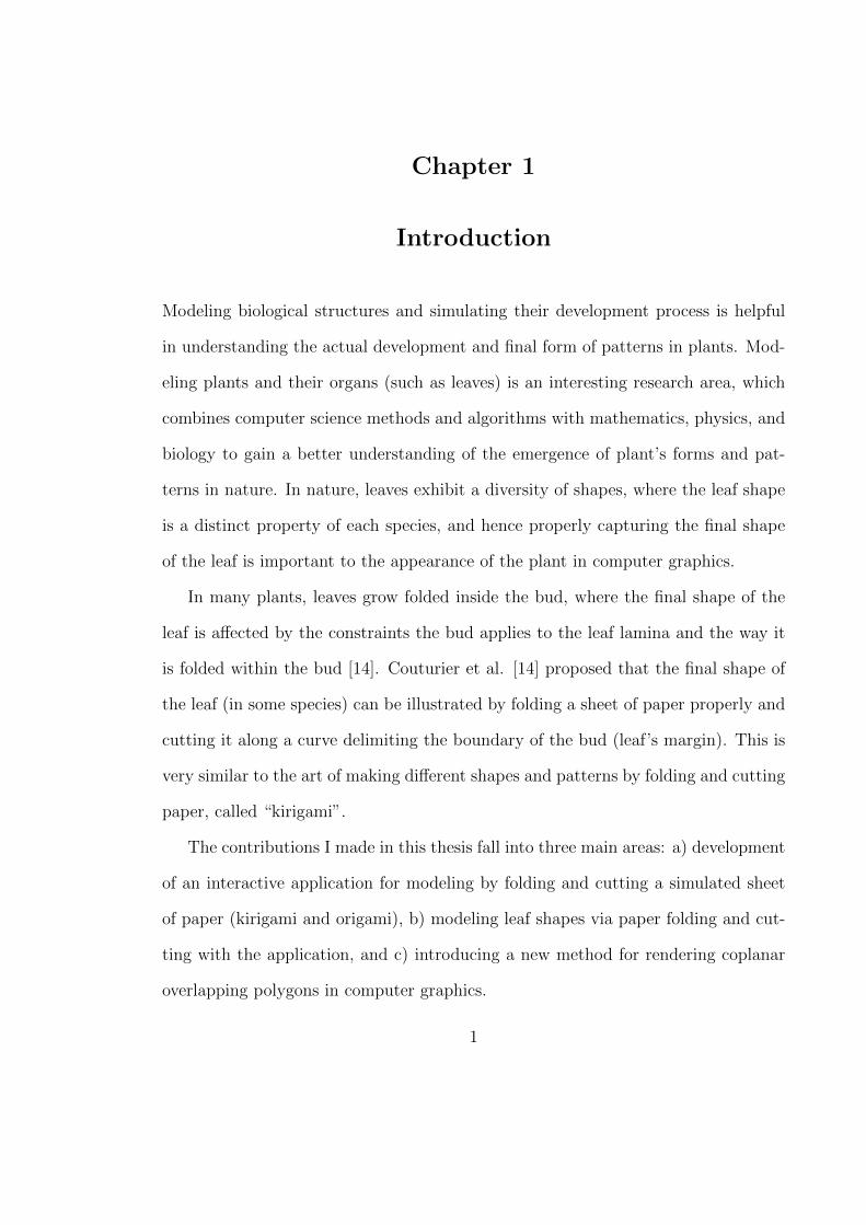
1.2 The process of modeling a three-lobed leaf shape with KiriSim byfolding a simulated sheet of paper (a-d), cutting it along the marginalcurve (e), and unfolding the final model(f). . . . . . . . . . . . . . . . 3

1.3 An origami butterfly (on the right), and a kirigami model (on theleft), both simulated with KiriSim. . . . . . . . . . . . . . . . . . . . 4

2.1 a) Valley fold (shown in red); b) Mountain fold (shown in blue); c)Tucking fold . . . . . . . . . . . . . . . . . . . . . . . . . . . . . . . . 7

2.2 Prayer fold (images from [8]). . . . . . . . . . . . . . . . . . . . . . . 82.3 Petal fold (images from [8]). . . . . . . . . . . . . . . . . . . . . . . . 92.4 Folding a bird base and shaping it into a crane (images redrawn from

[23]) . . . . . . . . . . . . . . . . . . . . . . . . . . . . . . . . . . . . 102.5 The base for a lizard with four legs, head, body, and tail. The shadow

tree is projected onto the x-y plane (Images redrawn from [23]). . . . 112.6 Cutting a star from a folded paper: Fold the paper to line up all edges

of the star, and then cut the paper along that line. . . . . . . . . . . 122.7 Shrinking edges of the graphs to obtain the straight skeletons. Edges

of the graph are drawn in black, and the straight skeleton is repre-sented in red. The trajectory is demonstrated by dashed lines (Imagesredrawn from [23]). . . . . . . . . . . . . . . . . . . . . . . . . . . . . 13

2.8 The crease pattern for “H” shape. The red and blue lines representvalley and mountain creases respectively. The line encircled with greenis the perpendicular. . . . . . . . . . . . . . . . . . . . . . . . . . . . 14

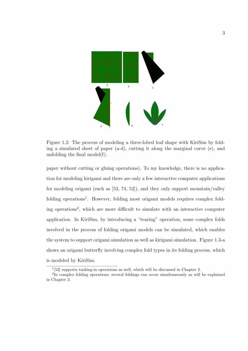
3.1 Different types of leaves (images from [66]). . . . . . . . . . . . . . . . 213.2 Leaf classification based on their venation pattern: a) veins run par-

allel to each other, b) veins diverge along the midrib, and c) veinsdiverge from the petiole. . . . . . . . . . . . . . . . . . . . . . . . . . 22

3.3 A three-polygon structure hinged along anti-veins for modeling mapleleaves (image from [12]). . . . . . . . . . . . . . . . . . . . . . . . . . 26

3.4 Leaves of beech and the miura-origami model for the leaf (images from[44]). . . . . . . . . . . . . . . . . . . . . . . . . . . . . . . . . . . . . 28

vii

3.5 Making the central part of a Cacalia yatabei with paper. a) Fold thepaper along OC, b, c) fold the paper along dotted line, d, e) separatethe layers and push in C into the bounding faces, f) cut the paperalong a line that passes from C, P, and Q, and unfold the paper. Theactual crease pattern for the leaves as in nature is represented in thegreen rectangle. . . . . . . . . . . . . . . . . . . . . . . . . . . . . . 29

3.6 Palmate leaves with different number of lobes (on the top). They arecollapsed into simple curves after being folded back (on the bottom)(images from [14]). . . . . . . . . . . . . . . . . . . . . . . . . . . . . 30

3.7 a) A rectangular sheet of paper with five folds which are all originatedat the petiole. b) The folded paper is is cut along a straight line withscissors. c) The sheet is unfolded. Folds correspond to sinuses andlobes. d) The sheet is folded with secondary folds. e) The sheet iscut. f) The sheet is unfolded. Secondary folds correspond to secondarylobes (Images from [15]). . . . . . . . . . . . . . . . . . . . . . . . . . 31

3.8 Geometric relationship between two successive lobes and sinuses, calledthe kirigami property, is represented in a5 and b5. “Length ratio(Ra/Rc) of two consecutive main veins is a function of the difference(α - β) between the angles they make with the anti-vein. Length ratio(Rb/Rd) of two consecutive main anti-veins is a function of the differ-ence (β - γ) between the angles they make with the vein” [15] (Imagesfrom [15]). . . . . . . . . . . . . . . . . . . . . . . . . . . . . . . . . . 32

4.1 Top image shows the fold line specified on the diagonal of the squareby the user (the red line). The bottom image shows the simulatedpaper folding along that line. . . . . . . . . . . . . . . . . . . . . . . 35

4.2 Illegal folding/unfolding operations. a,b) The paper is folded alongAB, and then it is folded along CD. If it is unfolded along AB, wherepolygons p1 and p2 should be moved: self-penetration occurs. c)The paper is folded along AB, d) it is unfolded along AB, and a foldoperation along QM is applied to polygon PQMB: the paper will bestretched at point B, because point B is shared by SABH and QMBP,and it is fixed in polygon SABH, but it moves in polygon QMBP. . . 36

4.3 If the user applies a fold operation along CD (a), both P and Q aresplit and folded (b). In order to only fold Q along CD, the user unfoldsthe paper along AB (c), applies a fold operation to Q along CD (d),and then refolds the paper along AB (e). . . . . . . . . . . . . . . . . 37

viii

4.4 a) The desired crease pattern for an origami ship, b) tucking in thepaper, c) the origami ship. d-h) Simulating a “tucking” operationwith a combination of folding and tearing operations to build a shipwith a paper. d-e) The initial paper is folded along OP, f) the paperis cut along ON, g) two folding operations are performed along QNand MN, h) the last fold is performed along PN to get the origamishape. . . . . . . . . . . . . . . . . . . . . . . . . . . . . . . . . . . . 38

4.5 Straight-cut tool (mixed fold and cut operations). Sequence of op-erations is demonstrated in the top of the figure. The “straight-cut”operation is magnified (in the bottom). The red circle is a point insidethe area that remains after the cut. . . . . . . . . . . . . . . . . . . . 40

4.6 Cutting the folded paper. First, model is folded (a,b,c, on the left).Then, a B-spline curve is specified (top-right). Finally, the model iscut and unfolded (bottom-right). Further explanations in the text. . . 42

4.7 KiriSim’s interface. . . . . . . . . . . . . . . . . . . . . . . . . . . . . 43

5.1 Polygons 1 and 2 are produced after applying ”Fold A” operation,polygon 2 is affected with respect to fold A and polygon 1 is fixed.Polygons 3 and 4 are produced from ”Fold B” operation, polygon 3and 1 are fixed, and polygon 4 is affected with respect to fold B.Polygons 5 and 6 are produced from ”Fold C” operation, polygon 5and 1 are fixed, polygon 4 and 6 are affected with respect to fold C.Polygons 1, 4, 5, and 6 are leaf polygons. The binary tree structureshows the parent-child relationships. . . . . . . . . . . . . . . . . . . 48

5.2 Multiple layer-sets in a folded paper. There are five layer-sets (L1,..,L5)with their normals shown by red arrows (on the left). Each layer-sethas a corresponding face list (on the right). . . . . . . . . . . . . . . 49

5.3 View plane and view direction are represented. Point v is the viewpoint. The affected polygons are folding down with respect to the viewpoint on the left, and folding up on the right. The ”view-transition”state is shown in red rectangles. . . . . . . . . . . . . . . . . . . . . . 50

5.4 Splitting a convex polygon by a line. Degenerate cases (b and c) aretreated differently. . . . . . . . . . . . . . . . . . . . . . . . . . . . . 52

5.5 Determining moving faces. The initial paper (a) is folded along L1(b). Then, the paper is folded along L2 (c), where faces Q and F arethe moving faces. Those faces with all their vertices located on theselected side of H are moving faces (d). . . . . . . . . . . . . . . . . 54

ix

5.6 Food-fill algorithm. The black pixels specify the boundary of the areaand the red pixel is the initial node inside the area. In each step theblue pixel is processed and the red pixels (the blue pixel’s neighbor)are marked as inside nodes. This process continues until no unmarkedpixel is left inside the area. . . . . . . . . . . . . . . . . . . . . . . . 55

5.7 Origami crafts. The paper has different colors on its two differentsides and the model conceptually contains coplanar faces with overlap-ping areas.Image taken from: http://crafts.iloveindia.com/origami-crafts.html . . . . . . . . . . . . . . . . . . . . . . . . . . . . . . . . 57

5.8 a) The folding steps are shown. b) The simplified 2D representationof the folded paper, c) paper is partially unfolded along L2, d) themodel is partially unfolded along L1: self-penetration occurs. . . . . 58

5.9 Rendering coplanar faces with overlapping areas. Narrow strips areused to separate two faces (a,b). (Images redrawn from [75]) . . . . . 59

5.10 Miyazaki’s technique for face order renewal. Three predefined foldtypes (a-c) and the order of faces after folding. Bold lines representthe moving faces. In “a”, new face stacks will be created, while in “b”and “c” the existing stacks are updated.(Images redrawn from [53]) . 60

5.11 Circular ordering of faces; A is above B, B is above C, C is above D,and D is above A.(Images from [28]) . . . . . . . . . . . . . . . . . . 61

5.12 a) A simple crease pattern, b) a side view of the folded paper, c) theOR matrix for this configuration.(Images from [52]) . . . . . . . . . . 62

5.13 A folding operation is performed and a new layer-set is generated (a-b), view-transition occurs and layer-sets are updated (b-c), L1 andL2 are merged to a single layer-set (d), view-transition occurs dueto rotation and layer-set is updated (e), and unfolding operation isperformed which results in separation of layer-sets (f). . . . . . . . . . 64

5.14 Phase A of algorithm only sorts polygons locally in each layer-set. Inthe top, the folding sequence is presented from left to right. Dependingon the geometry (size of the polygons) we will end up in case a or b. . 65

5.15 Basic idea of phase B. In blue rectangle the folding process is demon-strated. In the bottom, visible parts of each line segment (faces in3D) are marked by “A”, “B”, and “C”. . . . . . . . . . . . . . . . . . 66

5.16 Efficient version of phase B of the algorithm. Window’s start-pointand endpoint are represented by blue arrays, split results in list R arerepresented by green lines. a) l2 is split by S1; b) window is updated,l3 is split by S2; c) window is updated, l4 is not split at all; d) l5 issplit by S1; e) Each line in R makes a single group, which results infour groups . . . . . . . . . . . . . . . . . . . . . . . . . . . . . . . . 68

x

5.17 Phase B of algorithm, n = 5: a) l2, l3, l5 are split by horizontal dashedlines. b) l3, l4, l5 are split by dashed lines. c) l4, l5 are split by dashedlines. d) l5 is split by dashed lines. e)line segments are classified intogroups 1-4. . . . . . . . . . . . . . . . . . . . . . . . . . . . . . . . . 70

5.18 a) Best case, only one group results from phase B of algorithm; b)Worst case, seven groups result from phase B of algorithm. . . . . . 72

6.1 Common data structure used in origami applications (the folding op-erations and the crease pattern is shown in the top): a) hierarchy offaces, b) hierarchy of edges, c) list of operations with the ordered listof faces, d) vertex list (“C” in the vertex list represents the locationof the vertex after each operation if it moves and the initializationcolumn shows which vertices initially existed in the model with C astheir initial location). Further explanation in the text. . . . . . . . . 76

6.2 The employed data structure in KiriSim. a) the folding operationsand the crease pattern is shown, b) the corresponding hierarchicalface-vertex structure, c) the layer-set for the current configuration, d)the fold-lines, their creases, and the affected and produced faces withrespect to each fold-line. . . . . . . . . . . . . . . . . . . . . . . . . . 78

7.1 Different venations patterns require different modeling processes (mainveins are represented in red, anti-veins in blue). a) The petiole is lo-cated on one of the initial edges of the square sheet of paper. b)The petiole is located somewhere in the middle area of the paper. c)Secondary veins exist in the leaf (it is possible that case b and c arecombined in a leaf’s venation pattern). . . . . . . . . . . . . . . . . . 83

7.2 Modeling steps for a simple palmate leaf with no secondary lobes. . . 847.3 Modeling steps for a leaf in which petiole is located higher than the

bottom edge of the initial square sheet of the paper. . . . . . . . . . . 857.4 Modeling steps for a palmate leaf with secondary lobes. . . . . . . . 867.5 A maple leaf. The secondary lobes marked with circles can not be

captured by folding and cutting a paper. The red line (L1) is an anti-vein, which is not co-linear with the bisector of the sinus (L2) (imagefrom [15]). . . . . . . . . . . . . . . . . . . . . . . . . . . . . . . . . 87

7.6 Image and model of an Acer pseudoplatanus leaf, Sapindales, fromleft to right in the top. Image and model of a Fatsiajaponica leaf,Apiales, from left to right in the bottom (images from [15]) . . . . . 89

7.7 Image and model of an Acer leaf, from left to right in the top. Imageand model of a Sweet gum leaf, from left to right in the bottom. . . . 90

xi

7.8 Image and model of a Ribes Nigrum leaf, Saxifragales, from left toright in the top. Image and model of Acer pseudoplatanus leaf, Sapin-dales, from left to right in the bottom (images from [15]). . . . . . . . 91

7.9 A maple leaf modeled with KiriSim. Secondary lobes are ignored inthe top, and secondary lobes are considered in the bottom (From leftto right: the image of the real leaf, the modeled leaf with a junglegreen texture, image from [15]). . . . . . . . . . . . . . . . . . . . . . 92

7.10 A maple leaf modeled with KiriSim. Secondary lobes are ignored inthe top, and secondary lobes are considered in the bottom (From leftto right: the image of the real leaf, the modeled leaf with a junglegreen texture). . . . . . . . . . . . . . . . . . . . . . . . . . . . . . . 93

7.11 A bird modeled with KiriSim, and the corresponding modeling process(Mountain folds are represented in blue, valley folds in red, adding anew edge operation in yellow, and tearing in white). Further expla-nation in text. . . . . . . . . . . . . . . . . . . . . . . . . . . . . . . . 94

7.12 An insect modeled with KiriSim which requires a prayer fold (a-c),and its corresponding modeling process. . . . . . . . . . . . . . . . . 96

7.13 A frog modeled with KiriSim (in the top right), a photo of the realmodel (in the top left), and the crease pattern (in the bottom). . . . 97

7.14 A butterfly modeled with KiriSim (in the top right), a photo of thereal model (in the top left), and the crease pattern (in the bottom). . 98

7.15 Simple origami models, which are made by a sequence of mountainand valley folding operations (on the left), and the crease patterns (onthe right). . . . . . . . . . . . . . . . . . . . . . . . . . . . . . . . . . 99

7.16 A cup, a Samurai hat, and a heart modeled with KiriSim (on theright), and their crease patterns (on the left). . . . . . . . . . . . . . 100

7.17 Origami models which only consist a sequence of mountain and valleyfolding operations, and a single tucking operation (on the left), andthe crease patterns (on the right). . . . . . . . . . . . . . . . . . . . . 101

7.18 A kirigami model simulated with KiriSim. a-f) folding the paper,while in step “c” a straight cut operation along L, and in step “f” afinal cutting curve operation is performed. g) The final model withits crease pattern. . . . . . . . . . . . . . . . . . . . . . . . . . . . . . 102

7.19 A kirigami model simulated with KiriSim. Folding the paper andcutting it along the specified curve (in the top), and the final model(in the bottom). . . . . . . . . . . . . . . . . . . . . . . . . . . . . . . 103

7.20 A kirigami model simulated with KiriSim. a-d) Folding the paper, d)one “straight cut” operation followed by a final “cutting along curve”operation is performed. e) The final model with crease pattern. . . . 104

xii

7.21 THE END. All the characters (T, H, E, N, D) are generated byKiriSim, based on “one straight cut” theory by Demaine [23]. . . . . . 105

xiii

Chapter 1

Introduction

Modeling biological structures and simulating their development process is helpful

in understanding the actual development and final form of patterns in plants. Mod-

eling plants and their organs (such as leaves) is an interesting research area, which

combines computer science methods and algorithms with mathematics, physics, and

biology to gain a better understanding of the emergence of plant’s forms and pat-

terns in nature. In nature, leaves exhibit a diversity of shapes, where the leaf shape

is a distinct property of each species, and hence properly capturing the final shape

of the leaf is important to the appearance of the plant in computer graphics.

In many plants, leaves grow folded inside the bud, where the final shape of the

leaf is affected by the constraints the bud applies to the leaf lamina and the way it

is folded within the bud [14]. Couturier et al. [14] proposed that the final shape of

the leaf (in some species) can be illustrated by folding a sheet of paper properly and

cutting it along a curve delimiting the boundary of the bud (leaf’s margin). This is

very similar to the art of making different shapes and patterns by folding and cutting

paper, called “kirigami”.

The contributions I made in this thesis fall into three main areas: a) development

of an interactive application for modeling by folding and cutting a simulated sheet

of paper (kirigami and origami), b) modeling leaf shapes via paper folding and cut-

ting with the application, and c) introducing a new method for rendering coplanar

overlapping polygons in computer graphics.

1

2

Figure 1.1: Computer model of a palmate leaf: A) folded as in the bud; B) partiallyunfolded; C) completely unfolded.

To my knowledge, there is no computer graphics application for simulating and

visualizing the modeling of leaf shapes employing the paper folding and cutting

approach. The main objective of this thesis is to explore analogies between leaf

development and kirigami via development of a program called “KiriSim” (Kirigami

Simulator). “KiriSim” is an interactive computer graphics application, which allows

the user to visualize the process of folding and cutting a simulated sheet of paper to

model leaf shapes. Figure 1.1 shows a leaf modeled with KiriSim [60]. To model leaf

shapes with KiriSim, the simulated sheet of paper is folded interactively by the user,

and then a cutting curve specified by a B-spline (also drawn interactively) is applied

to the model. After the model is cut along the curve, it can be unfolded to get the

final shape of the leaf. The modeling process for a three-lobed leaf by KiriSim is

illustrated in Figure 1.2.

In addition to modeling leaf shapes, KiriSim can be used for creating some

kirigami and origami models (modeling traditional origami only involves folding a

3

Figure 1.2: The process of modeling a three-lobed leaf shape with KiriSim by fold-ing a simulated sheet of paper (a-d), cutting it along the marginal curve (e), andunfolding the final model(f).

paper without cutting or gluing operations). To my knowledge, there is no applica-

tion for modeling kirigami and there are only a few interactive computer applications

for modeling origami (such as [53, 74, 52]), and they only support mountain/valley

folding operations1. However, folding most origami models requires complex fold-

ing operations2, which are more difficult to simulate with an interactive computer

application. In KiriSim, by introducing a “tearing” operation, some complex folds

involved in the process of folding origami models can be simulated, which enables

the system to support origami simulation as well as kirigami simulation. Figure 1.3-a

shows an origami butterfly involving complex fold types in its folding process, which

is modeled by KiriSim.

1[53] supports tucking-in operations as well, which will be discussed in Chapter 2.2In complex folding operations, several foldings can occur simultaneously as will be explained

in Chapter 2.

4

Figure 1.3: An origami butterfly (on the right), and a kirigami model (on the left),both simulated with KiriSim.

In many computer graphics applications [53, 27, 28, 52, 75, 26, 73, 24, 13, 42,

43, 74] developed for origami modeling and visualizing, paper thickness is ignored,

which means a model may consist of sets of coplanar overlapping faces (the butterfly

in fig.1.3). In particular, z-buffer methods fail to deal with the problem of properly

rendering coplanar overlapping polygons since all these polygons have the same depth

values. There are a few approaches to deal with this problem [75, 28, 53], but I have

proposed and implemented a robust technique rooted in computational geometry.

This algorithm finds the visible areas (to the viewer) of each existing polygon in the

model based on the rendering order of the polygons, and only renders these visible

portions of the polygons (explained in Chapter 5).

1.1 Organization of Thesis

In this thesis, chapters are organized as follows. In Chapter 2, I discuss the related

work done in the area of modeling with paper and visualizing the models in comput-

5

ers, in particular origami and kirigami modeling. In Chapter 3, the previous work

relevant to modeling leaf shapes is discussed and different modeling approaches in

this area are reviewed. An introduction to “KiriSim”, the defined operations in this

system, and its interface is provided in Chapter 4. Chapter 5 describes the algo-

rithms employed in this thesis to develop the application. In Chapter 6, the data

structure used in the system, the implementation issues which I had to deal with

during development, and the tools and languages used are discussed. In Chapter 7,

some models which are simulated with KiriSim are demonstrated (including models

of different leaves and some origami models), and the modeling process for some of

them is illustrated. Finally, Chapter 8 provides a brief summary of my research and

discusses the potential directions for future work.

Chapter 2

Related Work: The Art of Modeling with Paper

In this chapter, an introduction to origami and kirigami, which are Japanese arts

of modeling things with paper, is provided. Then, different computer programs

that have been developed for paper manipulation and folding, mainly for origami

purposes, are reviewed.

2.1 Origami

Origami is the art of folding papers into sculptures of animals, plants, human figures,

and variety of other shapes. The Japanese word “origami” is the combination of

“oru,” which means “fold,” and “kami”, which means “paper” [23]. It is not clear

when or where the art of paper folding started, but it is believed that first attempts at

paper folding had to have coincided with the invention of paper in China, around 100

BCE [34]. In traditional origami, the initial sheet of paper should be convex, which

is usually in a square or a rectangular shape. Also, it is forbidden to use scissors

or glue in origami [26]. Origami has been the subject of many studies from both

artistic and mathematical perspectives. Mathematical studies of origami have led to

a topic called “computational origami”. Computational origami is a recent topic in

computer science, which focuses on efficient algorithms for solving origami problems

6

7

Figure 2.1: a) Valley fold (shown in red); b) Mountain fold (shown in blue); c)Tucking fold

such as “origami foldability”1 and “origami design”2, the two main problems in the

computational origami. Extensive work has been done in computational origami

area [18], however, further discussion in computational origami is out of the scope of

this thesis. Some terms which are frequently used in origami and in this thesis are

explained next.

2.1.1 Terminology

One can classify the folding types in origami roughly into three categories based on

the difficulty of fold: a) simple folds: mountain/valley, b) low-intermediate folds:

such as inside reverse fold (tucking), prayer fold, squash fold, rabbit-ear fold and c)

intermediate folds: such as petal fold. A valley fold is formed when the paper is

folded towards the viewer, which is represented by red lines in this thesis (fig.2.1).

1Initially given a specified crease pattern, marked with mountains and valleys, origami foldabilityis used to investigate whether or not the crease pattern can be folded into origami [18].

2In origami design, the goal is to fold a piece of paper into an object with specified propertiesand configurations.

8

Figure 2.2: Prayer fold (images from [8]).

A mountain fold is formed when the paper is folded away from the viewer. The

mountain folds are represented by blue lines in this thesis (fig.2.1). In cases b and c,

folding of multiple creases occur simultaneously. Tucking or inside reverse fold can

be seen as a combination of two mountain folds followed by a valley fold (fig.2.1). In

other words, tucking-in folds a face to the inside direction bounded by certain faces

[53]. Prayer fold and petal folds are illustrated in Figures 2.2 and 2.3 respectively.

The focus of this thesis is on the models that can be made with the two first category

of foldings (cases a and b).

Crease pattern is a division of the paper into a finite set of polygonal regions by

all the mountain and valley folds existing in the final model. Each line segment in

the crease pattern is called a crease. Each polygon, bounded by the creases and the

edges of the square, is called a facet of the crease pattern [46]. A vertex in the crease

9

Figure 2.3: Petal fold (images from [8]).

pattern is either a corner of the paper or a vertex of the facets. A valley-mountain

fold should not be confused with a valley/mountain crease. By a valley/mountain

fold, the paper is folded along a single line, and this fold generates creases on all

folded layers of the paper (If the paper is unfolded, some of these creases may be

mountain creases, some may be valley creases from the current view point) [8].

A base is an origami form at an intermediate stage of folding, which can be

relatively easily shaped to the final origami model (fig.2.4). There are a limited

number of handful origami bases, and various models can be made from the same

base [18, 23, 74]. A flat-foldable crease pattern is any crease pattern that can be

folded into an origami so that all faces of the model lie in a common plane [46],

and the flat origami model is “the one which can be pressed into a book without

introducing new creases” [33].

10

Figure 2.4: Folding a bird base and shaping it into a crane (images redrawn from[23])

A shadow tree is a tree with cyclically ordered leaves and no root, with specified

edge lengths. Each edge is the projection of a region in the base, called “flap”

(fig.2.5). Lang [46] defines a flap as a group of facets in a base that project to a

common edge of the tree graph. Flaps can be rotated around “hinges”, which are

the vertical creases in the base projected into internal nodes of the tree (fig.2.5).

2.2 Kirigami

Very similar to the widely known art of origami, another paper art, known as

kirigami, combines both folding and cutting to create artistic models out of a sheet

of paper. In ancient times, kirigami was used to cut out the sculptures of Samurai

families [50]. Like origami, kirigami can also be studied from both mathematical

and artistic perspectives. Erik Demaine has extensively explored mathematics of

kirigami, entitled as “one straight cut” problem1 [17, 21, 22, 20, 16, 23].

1Demaine discussed this problem in the computational origami category.

11

Figure 2.5: The base for a lizard with four legs, head, body, and tail. The shadowtree is projected onto the x-y plane (Images redrawn from [23]).

2.2.1 One Complete Straight Cut

Folding a sheet of paper flat, and then making one straight cut along the folded

paper results in two or more separate polygonal shapes. “Given a planar graph1 with

straight edges on a piece of paper, one can investigate if the paper can be folded flat

so as to map the entire edges of the graph to a common line and map nothing else

to that line” [23]. This is known as the “one straight cut” problem. Interestingly,

Demaine proved that every polygonal shape (including multiple disjoint, nested, and

adjoining polygons) can be produced by folding and one straight cut [21, 22, 20, 16].

There are two solutions for the fold and cut problem: “straight skeleton”, and

“disk-packing”. The “straight skeleton” solution, which is based on capturing sym-

1In here, the term graph is referring to a polygonal shape (including multiple disjoint, nested,and adjoining polygons), where polygon vertices are graph nodes, and polygon edges are edges ofgraph.

12

Figure 2.6: Cutting a star from a folded paper: Fold the paper to line up all edgesof the star, and then cut the paper along that line.

metries in the target polygonal pattern [23, 17], will be discussed in more detail

in the following subsection as it is more straightforward. The interested reader is

referred to [23, 11] for more details on “disk-packing” solution.

Straight Skeleton Method

The straight skeleton method was proposed by Demaine et al. [22]. It is an algorithm

which calculates the crease pattern that lines up all edges of the polygonal shape

in a plane. The straight skeleton consists of several line segments, where each of

them locally aligns a pair of polygon edges (graph edges) [19]. The straight skeleton

definition is as follows: “Suppose we simultaneously shrink each polygon in such

a way that the edges retain their orientation, and the perpendicular distance from

every shrunken edge to corresponding original edge is the same for all shrunken

edges. The straight skeleton is the union of the trajectories of all vertices during the

shrinking process” (fig.2.7) [23].

However, for most graphs the straight skeleton itself is not sufficient to line up all

the edges, and additional type of creases named “perpendiculars” are required to fold

13

Figure 2.7: Shrinking edges of the graphs to obtain the straight skeletons. Edges ofthe graph are drawn in black, and the straight skeleton is represented in red. Thetrajectory is demonstrated by dashed lines (Images redrawn from [23]).

the paper in a way that lines up all graph edges, in addition to the straight skeleton

(each perpendicular edge passes through a skeleton vertex and is perpendicular to a

graph edge). Figure 2.8 shows an example of the straight skeleton of a graph and

the perpendiculars which are necessary to fold the graph on a single line.

2.3 Computer-Assisted Paper Manipulation for Folding Origami

In order to fold an origami, the process of folding has to be clear. Orizu, which is

a diagram to show the folding process, or videos can be used to fold an origami.

However, interactivity is not involved in these manuals and it may be difficult for

the trainee to understand and fold a model [27]. In addition, due to paper thick-

ness, folding multi-layered models can be quite cumbersome, and the paper can get

crumpled after several trials. Also, it may be difficult to re-build the model.

Using computers to model, visualize, and possibly animate origami can solve

these problems. The virtual paper can be folded as many times as desirable, and

14

Figure 2.8: The crease pattern for “H” shape. The red and blue lines represent valleyand mountain creases respectively. The line encircled with green is the perpendicular.

depending on the application, the model can be viewed from different directions in

3D. Additionally, it may be possible to undo the previous steps without ending up

with a crumpled paper. However, many issues can arise while developing a computer

program as a tool for modeling accurate and realistic origami models. These include

modeling non-planar surfaces created during the folding process (as in modeling

with real paper), maintaining the order of layers in a flat-folded model for rendering

purposes, and collision detection to avoid paper self-penetration. It is also difficult

to come up with a user friendly interactive interface, which would allow the user to

do all the possible folding types existing in origami models. In recent years, several

computer applications have been developed for folding origami models which will be

reviewed in this section.

15

2.3.1 Non-interactive Applications

Several applications have been developed only for instructional purposes on designing

and/or creating paper models. [37, 1, 3]. For example, “Paper animal workshop”

[1] is an origami software which is used for teaching origami by animation, folding

instructions, and by presenting the crease patterns.

Other applications have been developed mainly for the purpose of animating

origami models’ folding processes. Agui et al. [7] developed a system for animating

origami folding by calculating the coordinates of the polygons in the origami model

and giving them as key-frames to the system. Furuta et al. proposed a spring-mesh

model for 3D origami animation [27]. In this model, faces are represented by spring

networks, and because the system has flexibility due to having springs, it handles

non-rigid origami (in non-rigid origami faces can be deformed).

All the discussed systems so far require professionals to provide appropriate in-

put to the system, then use that information to animate and visualize the origami

folding process. A different approach for generating origami animation on comput-

ers is used by Kato et al. [42, 70], which is based on information extraction from

origami diagrams and images. The authors developed a system which first extracts

graphics elements of origami diagrams (i.e. illustrations, special symbols, sentences,

step numbers), then recreates the folding process and animates it in 3D. Another

image-based system was developed by Mitani [51] who employs a method for recog-

nizing and rendering origami from images. In this system, the structure of folded

paper is recognized from digital images, and the corresponding folding operations

are simulated and animated on the computer.

16

2.3.2 Interactive Applications

In interactive systems for origami modeling purposes, the user is allowed to design

and visualize origami models. TreeMaker is a tool capable of constructing full

mountain-valley crease assignments for a wide variety of origami bases [5]. The first

version of this computer program, which is in fact the implementation of the tree

method, was released by Lang. The user can set up flaps, their lengths, and their

angles which allows them to design origami bases that are more complicated than

anything a person could design by hand. By providing a stick figure as input (the

shadow tree), TreeMaker computes the full crease pattern for a base which, when

folded, will have a projection equivalent to the input shadow tree.

ORIPA is a program which folds origami based on the corresponding input

crease pattern [52]. ORIPA has an editor window that allows the user to draw the

crease pattern for the desired origami model on a simulated square sheet of paper

by specifying a set of valley and mountain creases. Then the system calculates the

folded shape based on the given crease pattern. In case the designed crease pattern

with the specified mountain-valley assignment is flat foldable, the folded origami is

visualized in a display window. Otherwise, the user is asked to modify the crease

pattern to a flat foldable one.

Both ORIPA and TreeMaker require the user to have a basic mathematical un-

derstanding of the origami models. In ORIPA, the user is expected to know the exact

crease pattern for the model, and in TreeMaker, he should know the corresponding

base for the final model. Additionally, the user should be able to extract the shadow

tree from the base.

17

Among interactive computer applications for creating origami models, some of

them do not require the user to have specific knowledge of origami. In such applica-

tions, an origami can be folded by interactive trial and error, or heuristic techniques

based on the folder’s intuition [45]. For example, Lang developed a simulator, where

a set of mountain-valley fold operations could be defined by manipulating a sheet

of paper in real time using mouse and keyboard. A corner or edge can be grabbed

and dragged to a desired position to fold the paper. However, only simple origami

models can be folded with this program, and the model can only be rotated in the

plane of the paper [4]. At the same time and quite similar to Lang’s work, Fastag

developed an interactive origami simulator called eGami [25].

One can fold many complicated three-dimensional origami models by an applica-

tion called Origami Simulator [53], using the three kinds of folding operations defined

in the system: bending, folding up1, and tucking in. The simulated sheet of paper

can be manipulated by the interactive process of picking and moving a corner vertex

of the paper using a mouse as in Lang’s model. In addition, a curving operation is

provided to curve the paper. Round faces are approximated by a set of ribbon-like

polygons where the roundness is calculated by minimizing an elastic energy function,

assuming the paper is constrained by a defined fixed floor plane. The front and back

of the paper can be visualized in different textures and the model can be viewed

from different directions.

There is another interactive system [74], that makes 3D animations of the model

while a sequence of folds are being performed interactively to allow the user to re-

build the model later. This application has two main features, making it different

1Folding up is a bending operation of 180 degrees.

18

from other similar computer programs: ”the ability to visualize overlapping faces”,

and “the halfway folding process”. In order to visualize the overlapping faces in 3D

and to make the multiple layers on top of each other visible, the origami model is

reconfigured by slightly moving apart these overlapping faces (polygons are rotated

along a rotation axis determined from figuration and overlapping relationships of

the faces). The halfway folding process is where the user can select an origami base

which is similar to his/her intended model, and then the system teaches the folding

process to fold the paper from a square to the specified base. After folding the base,

it can be shaped to the final intended origami model by the user.

Also, a system for creating origami models with a multi-touch approach was

developed by Chang, where origami models can be interactively manipulated on

tablets [13].

Another category of computer programs for folding origami are those that the user

interacts with the application by a set of pre-defined rules or commands which define

the folds. Kishi et al. [43] designed and developed an origami system which enables

web users to fold paper over the web. The system consists of an origami browser

and an origami editor. The user folds the paper by inserting a set of commands to

the editor and then can watch the folding process on the web browser. This origami

system handles only two basic fold types, mountain and valley, which makes it unable

to fold shapes such as cranes and frogs. In addition, I found it cumbersome to learn

the related commands.

An origami construction environment based on constraint functional program-

ming was proposed and implemented by Ida in 2003 [35]. In this method, basic

19

origami operations are described by six Huzita axioms1 by which 2D geometrical

objects can be constructed. The geometric properties of the paper folds are repre-

sented as systems of equations. Paper folding functions are invoked interactively, the

process of origami construction is driven by solving the systems of equations, and

the result is visualized after each fold is applied. A similar approach is employed by

Kasem to develop a web application for constructing and visualizing origami on a

web browser [41].

Origami design has also been explored from robotic manipulation perspective

[31, 9]. The world’s first origami-folding robot was presented by Balkcom, where a

machine is able to fold simple origami (flat origami models that only have mountain

and valley folds) [9]. Hawkes et al. [31] presented a self-folding origami made from

a programmable sheet, composed of interconnected triangular sections, in which the

sheet is folded to an origami model by providing appropriate set of commands.

1Having a set of points and lines, Huzita axioms are intended to capture which single new creasescan be constructed by alignment of a combination of these points and lines [23].

Chapter 3

Related Work: Modeling Leaf Shapes

Modeling biological structures and simulating the development of forms and patterns

found in living organisms is an active research area [57, 66], and different techniques

have been proposed to describe various organisms’ shapes in nature. These models

are helpful as visualizing the results of the simulations leads to better understanding

of the development and the final forms of these structures.

In plants, properly capturing the character of species is highly dependent on

representing the details of the plant’s form, such as the shape of the leaf. Leaves, the

vital organs of plants, exhibit a diversity of shapes in nature, and are important to

the visual appearance of the plant [65]. Thus, it is important to study the structure

and development of leaves and visualizing them properly. In this chapter, I will

outline the terminology used to describe the leaf forms first, and then, I will review

the related work on modeling leaf shapes.

Leaves are classified into “simple” and “compound” according to the shape of

the blade (fig.3.1). In simple leaves the blade is undivided (i.e. indentations do not

reach the midrib). Compound leaves have fully subdivided blades, and each division

is called a leaflet. Simple leaves are divided into three types: “entire”, “toothed”, and

“lobed”. The margin is smooth in entire leaves; toothed leaves have small serrations

in the margin; and in lobed leaves the blade is composed of lobes as a result of the

margin being deeply indented (but not divided) [66].

Leaves are also classified based on their venation patterns: “parallel-veined”,

20

21

Figure 3.1: Different types of leaves (images from [66]).

“pinnate”, and “palmate”. If the main veins run parallel to each other, then the leaf

is parallel-veined, while in pinnate leaves all the veins derive from the midrib or the

main vein which bisects the leaf, and in palmate or digitate leaves the veins diverge

radially like fingers in a hand (fig.3.2).

In the context of modeling leaves, one can distinguish different levels and styles

of description, such as geometric, bio-mechanical, and molecular (a model can be a

combination of these description levels). The methods employed in this thesis and

the main focus of this chapter is geometric techniques.

Some leaf modeling techniques are dynamic and simulate development and growth,

others only capture the final shape of the leaf, which is sufficient for computer graph-

ical purposes (static modeling techniques). In this chapter, I first review techniques

22

Figure 3.2: Leaf classification based on their venation pattern: a) veins run parallelto each other, b) veins diverge along the midrib, and c) veins diverge from the petiole.

that focus on leaf development (of different leaf types), and in the second section, I

focus on static modeling techniques for specifying leaf shapes.

3.1 Modeling Leaf Development

In one of the early attempts to model leaf growth, laminar development of simple

leaves was simulated by Scholten et al. [68]. In this method, a set of points, moving

outwards in each time step, mark the margin of the leaf. These points are initially

located on an ellipse or a circle, and their new location is determined based on the

growth center position on the midrib and the points’ current location. This process

is applied iteratively to get the final leaf shape.

One alternative technique for modeling leaf growth is employing time-dependent

surfaces. In this method, leaves are represented as a set of bi-cubic patches [62],

where the size and the shape of the leaf is changed in time by moving control points,

simulating the leaf development [59].

23

Physically-based techniques have also been employed in leaf modeling area [36,

76]. Two of the possible physical representations for simulating leaves are mass-

spring (elasticity) and fluid model. Wang et al. [76] employed a fluid model to

simulate the growth of plant leaves in 2D. In this model, the leaf is treated as a

viscous incompressible fluid, and they assume its growth is isotropic (there is no

preferential direction for leaf growth). In contrast to fluid technique, in which the

modeling is performed within a continuum, mass-spring model discretizes the tissue

into a set of polygons (or cells). The mass-spring modeling approach maintains

adjacent nodes, and it is able to simulate the effect of cell walls. Petals in opening

flowers were simulated and animated using mass-spring method by Ijiri et al. [36],

where each petal is represented as an elastic triangular mesh growing based on the

user specified parameters. This approach is based on differences in cell expansion

rate between the inner and the outer sides of the petal (there is an imaginary inner

surface which is used in regional growth computations assuming the petal thickness

is constant during opening).

The presence of the veins is considered and the venation pattern is modeled

in some of the leaf modeling techniques [67, 55, 32, 14, 39]. Runions et al. [67]

simulated the entire leaf blades along with modeling the venation pattern developing

in leaves. This biological-motivated approach for modeling leaf shapes is based on

the placement of auxin sources, development of veins, and leaf growth. An initial

leaf contour is defined interactively by a parametric curve which later changes as

the leaf blade grows in three possible ways: marginal growth, where the leaf edge

is scaled; uniform growth, where the entire leaf blade is scaled uniformly including

auxin sources and veins; non-uniform anisotropic growth, where the initial leaf shape

24

is deformed over time with user-defined functions. Furthermore, the initial nodes

(nodes are the elements that construct veins in this model) are located on the surface

of the leaf interactively by the user, and auxin sources which direct the veins to grow,

are located based on a version of dart-throwing algorithm [67]. [14, 39, 44] and [55, 32]

will be described in Section 3.2 since they only capture the final form of the leaf and

do not consider the leaf development.

L-systems are re-writing systems introduced by Lindenmayer for modeling plants

based on a recursive fashion. In L-systems, an object is represented as a string of

symbols which is rewritten in parallel using a set of rules [59], and a set of re-writing

expressions model plant growth over time. One of the earliest attempts to model

marginal leaf growth in lobed leaves employed deterministic L-systems, where the

lobes and sinuses in the leaf margin are represented by L-system symbols [69]. Several

extensions have been made to L-systems since the first time they were employed for

modeling plants [47, 58, 56]. Prusinkiewicz et al. [58] employed dL-system to model

and animate compound leaf growth, where leaflets are generated recursively. The

model starts from an apex which elongates according to a growth function, and

upon reaching a threshold length, a pair of leaflets are produced based on predefined

surfaces (bicubic patches). Then, the apex subdivides into an inter-node (leaflets are

separated by inter-nodes along the branching structure in compound leaves) and an

apex. During the development process, the length of the inter-nodes, the branching

angles, and the size of the leaflets gradually changes over time [58]. In addition, L-

systems can be employed to generate the venation structure of the leaves recursively,

which can be used for modeling different leaf types [59].

A different approach which combines L-systems and genetic algorithms [29] to

25

produce leaf shapes was employed by Rodkaew [63]. They use L-systems to generate

the skeleton of the leaf and then apply genetic algorithms to fix the parameters of

the L-systems rules in a way that the produced leaf best resembles a goal image of

the leaf.

3.2 Static Modeling of Leaves

Different techniques have been employed to model final leaf shapes. Some of these

techniques are based on the information extracted from real leaf images and the

modeling method tries to reconstruct the leaf shape from that data [61]. The other

techniques are either interactive, where the modeler guides the formation of the leaf

shape [55], or the leaf shape is automatically generated based on algorithms [64].

Some modeling techniques use images of real leaves and attempt to reconstruct

leaf shapes from the data extracted from the images. Quan et al. [61] employed

an image-based approach to model plants, specifically plants leaves. A set of 30

to 45 images taken from different angles is given to the system as input. A cloud

of 3D points is computed and the images are segmented to recover the geometry

of the individual leaves. To decrease errors due to overlapping leaves, the user

can refine segmentation (by splitting or merging the segments). Finally, the leaf is

reconstructed based on a deformable generic leaf model chosen manually by the user,

which can be manipulated to make the leaves look more realistic [61].

As mentioned in the previous section, many modeling techniques consider the

presence of veins as an important factor affecting leaf shapes. The remainder of this

section explores these techniques. Rodkaew [64] employed a particle based approach

26

Figure 3.3: A three-polygon structure hinged along anti-veins for modeling mapleleaves (image from [12]).

to model leaf shapes. Initially, some particles are randomly scattered on the given

leaf margin, and a target is set at the leaf petiole. The particles move toward a

direction determined by the target position and the position of the closest particle.

The trail of the particles determines the venation pattern of the leaf. The veins

become thicker near the petiole as particles join on their way to petiole.

To add leaves to the modeled maple trees, Bloomenthal et al. [12] mapped

leaf textures (extracted from images) to a three-polygon structure, and hinged the

polygons along some secondary veins (fig.3.3). Later, the polygons could be rotated

along the hinges based on the wind-direction which helped to achieve more realistic

models of maples trees.

Mundermann et al. [55] proposed a method for modeling lobed leaves, in which

the input to the system is the leaf silhouette extracted from an input image or

specified by the user. The branching skeleton of the two-dimensional silhouette is

then defined interactively or it is automatically generated by the system using a 2D

27

Voronoi diagram. Using inverse subdivision, the number of points on the skeleton is

decreased to a set of points which are used to convert it into a set of interconnected

“sticky splines”1. To construct the surface, a generating curve is swept between the

silhouette and the branching skeleton. The leaf model can be deformed freely in 3D

space using graphically defined functions that control the skeleton modification.

Hong et al. [32] developed an interactive modeling system, where the leaf silhou-

ette is extracted from the leaf image. The vein structure, which is represented as

a hierarchical collection of piecewise linear curves is identified interactively by the

user. A triangular mesh is automatically generated by the system to simulate the

leaf blade fitting the skeleton [32]. General cylinders are used to model veins, leading

in more realistic light and shadow effects.

Very similar to Hong’s system, Lu et al. [48] modeled and animated plant leaves

wilting due to insufficient amount of water. They also use triangular mesh to rep-

resent the leaf surface and the venation skeleton is generated interactively. The leaf

surface deformation is controlled by movement of the venation skeleton, where each

vertex in the skeleton is rotated along a fixed vector based on its association with

the skeleton.

Hammel et al. [30] used implicit contours to automatically generate leaf margins

around a branching skeleton, which was modeled using L-systems capturing layout

of lobes. An implicit contour is the set of all the points (x,y), where f(x,y) = c.

Constant c is a threshold value and f(x,y) is a field function. The value of the field

function at any point is equal to the sum of contributions from all skeletal elements.

1Sticky splines are able to maintain topological relations between different interconnected splinecurves while being edited.

28

Figure 3.4: Leaves of beech and the miura-origami model for the leaf (images from[44]).

Any point that evaluates to a number greater than c is considered to lie outside of

the contour [30].

A few modeling techniques consider the fact that in many plant species leaves

are folded inside the bud, and try to model the leaves with paper folding and cutting

(origami and kirigami as explained in Chapter 2) [44, 38, 14]. Inspired by obser-

vation that leaves of hornbeam and beech have regular corrugated folding patterns,

Kobayashi et al. [44] numerically simulated the unfolding mechanism based on a

paper model called “Miura-Ori”, with mountain and valley creases. This approach

employs a vector analysis method to determine the location of all creases and inter-

section points in three-dimensional space while the leaf is being unfolded, based on

the leaf opening angle, the angles between the mid-vein and branching veins, and

the length of the veins. The proposed paper model is illustrated in Figure 3.4. A

problem with this model is that to fold the paper as shown (with the direction of

folds matching the folds in leaves), the direction of the folds on one side of the paper

29

Figure 3.5: Making the central part of a Cacalia yatabei with paper. a) Fold thepaper along OC, b, c) fold the paper along dotted line, d, e) separate the layers andpush in C into the bounding faces, f) cut the paper along a line that passes fromC, P, and Q, and unfold the paper. The actual crease pattern for the leaves as innature is represented in the green rectangle.

model is not consistent with the direction of the folds in leaves, which makes it is

necessary to bend the paper along the main vein.

Kaino [38, 39] observed that there is a relationship between the way digitate leaves

are folded inside the bud, their venation pattern, and the symmetric arrangement

of lobes and sinuses, and proposed an origami based model which employed folding

and cutting to generate leaf shapes such as maple. Figure 3.5 shows the folding and

cutting steps he proposes in his paper for modeling a leaf shape with three lobes

[38]. The problem with this modeled leaf is that the direction of folds (mountain

30

Figure 3.6: Palmate leaves with different number of lobes (on the top). They arecollapsed into simple curves after being folded back (on the bottom) (images from[14]).

and valley folds) is not consistent with the way the leaves are naturally folded inside

the bud, and the direction of the fold changes at one point in the middle of the main

vein (fig.3.5). The real crease pattern for a folded leaf is represented in Figure 3.5.

Couturier et al. [14, 15] has extensively studied the impact of the way the leaves

are folded inside the bud on their final shape. They observed that the constraints

the boundary of the bud imposes on the lamina while it is growing folded inside the

bud, and the way in which the leaf is folding within the bud affects and determines

the final shape of the leaf. Ignoring the three dimensionality of the bud and the leaf

thickness, which leads to 3D partially folded forms of the leaf within the bud, the leaf

margin can be collapsed into a simple curve when it is folded. By varying the angles

between veins and anti-veins, and changing the margin curve, different leaf forms

can be achieved (fig.3.6). The delimitation of the folded lamina by a curve is similar

31

Figure 3.7: a) A rectangular sheet of paper with five folds which are all originatedat the petiole. b) The folded paper is is cut along a straight line with scissors. c)The sheet is unfolded. Folds correspond to sinuses and lobes. d) The sheet is foldedwith secondary folds. e) The sheet is cut. f) The sheet is unfolded. Secondary foldscorrespond to secondary lobes (Images from [15]).

to the Japanese art of “kirigami”, where a sheet of paper is folded and cut (fig.3.7).

Focusing on palmate leaves, they geometrically analyzed the relationship between

the position of the folds, their length on the leaf surface, and the angles between

them (fig.3.8), called the “kirgami property” of leaves. To illustrate the kirigami

property, the triangle delimited by Ra and Rc (the lengths of the two main veins

on two adjacent lobes) and the perpendicular h to the leaf lamina is superimposed

(fig.3.8). The value of h is expressed as:

h = sin(p)Ra

Given that the sum of the angles of a triangle is π, one can write:

h = sin(p+ α)Rb

h = sin(p+ α− β)Rc

32

Figure 3.8: Geometric relationship between two successive lobes and sinuses, calledthe kirigami property, is represented in a5 and b5. “Length ratio (Ra/Rc) of twoconsecutive main veins is a function of the difference (α - β) between the angles theymake with the anti-vein. Length ratio (Rb/Rd) of two consecutive main anti-veins isa function of the difference (β - γ) between the angles they make with the vein” [15](Images from [15]).

33

By comparing the first and the last expressions, the following equation is achieved:

Ra

Rc

=sin(p+ α− β)Rc

sin(p)Ra

In Figure 3.8, the relation between γ and β is also shown, which corresponds to

angles and length ratios of two main anti-veins (whereas the above illustrations relate

the angles and length ratio of two main veins). The kirigami property shows that

the length of the veins and anti-veins is co-related with the angles between them,

and thus affecting the shape of the leaf margin since the veins and anti-veins are the

axes of symmetry of the contour.

The mathematical methods developed by Couturier et al. offer an excellent

paradigm for a new interactive program for modeling leaves, incorporating the advan-

tage of computational kirigami that I discussed earlier (e.g. unrestricted possibility

of folding many times). To my knowledge, no computer graphics application has

been developed to simulate this modeling approach. Thus, the main focus of this

thesis is to design and develop an application by which a simulated sheet of paper can

be folded in a particular way (consistent with the leaves folding in the bud), which

can then be cut along the leaf margin, and when unfolded, the model resembles the

leaf shape.

Chapter 4

The Kirigami Simulator (KiriSim)

In many plant species, leaves grow folded inside the bud, and after unfolding, they

preserve their shape till the end of development process (Chapter 3). Cuturier et

al. observed that there is a close relationship between the position of folds and

the venation pattern of the leaf, and the way the leaves are folded inside the bud

affects their final shape. Inspired by this observation, I have developed a program

named “KiriSim”, which is an interactive computer graphics application, designed

and implemented for modeling leaf shapes via kirigami. KiriSim allows the user to

fold a simulated sheet of paper interactively, and then cut the folded paper along a

user-specified curve. Finally, the user can unfold the paper to get the actual shape

of the leaf. In addition to modeling leaf shapes, KiriSim can be used as a tool for

modeling origami and kirigami.

In this chapter, an introduction to the system’s interface is provided, and the

basic operations that KiriSim supports are explained.

4.1 Folding the Simulated Paper

By selecting the “Manipulation” mode (fig. 4.1) and drawing fold lines, the user is

able to fold the simulated paper. The fold lines can be drawn by dragging the mouse

from the start point to the end point of the desired line segment on the simulated

paper. When the fold operation along the line is performed, some faces are rotated

34

35

Figure 4.1: Top image shows the fold line specified on the diagonal of the square bythe user (the red line). The bottom image shows the simulated paper folding alongthat line.

36

Figure 4.2: Illegal folding/unfolding operations. a,b) The paper is folded along AB,and then it is folded along CD. If it is unfolded along AB, where polygons p1 and p2should be moved: self-penetration occurs. c) The paper is folded along AB, d) it isunfolded along AB, and a fold operation along QM is applied to polygon PQMB: thepaper will be stretched at point B, because point B is shared by SABH and QMBP,and it is fixed in polygon SABH, but it moves in polygon QMBP.

along the line and other faces are fixed. It is possible to choose which faces will be

rotated in two ways: a) the user selects a point on one side of the line and all faces on

that particular side will be moved, or b) the user selects all faces on one side of the

line, which are supposed to be moved1. To choose any of these options, the “Select”

mode is enabled, and then either “Polygon” or “Point” options are selected for case

“a” and “b”, respectively (fig.4.7 items E2 and E4). Finally, the “fold” button should

be pressed to fold the paper along that line, which is animated and visualized on the

screen. The fold type, either mountain (anticlinal) or valley (synclinal) (see Chapter

2 on origami fold types), can be customized in the “Setting” tab before pressing the

1The user should be careful to select all the faces on that side since the system does not checkfor the possible mistakes in polygon selection.

37

Figure 4.3: If the user applies a fold operation along CD (a), both P and Q are splitand folded (b). In order to only fold Q along CD, the user unfolds the paper alongAB (c), applies a fold operation to Q along CD (d), and then refolds the paper alongAB (e).

fold button (fig.4.1).

Each fold angle can be customized by the sliders in the “Sliders” tab in the side

bar, which are dynamically added to the interface for each new fold line. It is possible

to partially unfold the paper along some fold lines, as long as the user is careful

about avoiding the folding/unfolding operations that lead to the self-penetration of

the simulated paper (fig.4.2 a,b), or cause the paper to stretch (fig.4.2 c,d).

When a fold line segment is drawn and the fold operation is performed, all the

faces intersecting with this line segment will be split by it. For example, in Figure

4.3a,b, when the fold line CD is applied both polygons P and Q are folded along

CD. If the user wishes to only fold some specific polygons (e.g. polygon Q along CD

in Figure 4.3), he must unfold the paper so that the fold line can be only applied to

those polygons. For instance, in Figure 4.3, the model is unfolded along AB, then

a new fold line is drawn on polygon Q so that it does not overlap with any part of

38

Figure 4.4: a) The desired crease pattern for an origami ship, b) tucking in the paper,c) the origami ship. d-h) Simulating a “tucking” operation with a combination offolding and tearing operations to build a ship with a paper. d-e) The initial paperis folded along OP, f) the paper is cut along ON, g) two folding operations areperformed along QN and MN, h) the last fold is performed along PN to get theorigami shape.

polygon P. After performing the fold operation, the model can be refolded (fig.4.3

e).

4.2 Tearing the Simulated Paper

By introducing the tearing operation to the system, one can decompose complex

fold operations (explained in Chapter 2) to a set of folding and tearing operations1.

1Eventually, there is no need for gluing after tearing the paper, since it does not make anydifference in the final appearance of the model, and if the torn edges are glued, it might be impossibleto unfold the model partially due to connectivity.

39

Consequently, a wider range of models can be simulated by KiriSim, but the user

needs to figure out where to tear the paper, and how to modify the folding process to

get the correct final model. For example, Figure 4.4 shows how the tearing operation

combined with simple mountain and valley folds can simulate a tucking operation,

needed to create the origami ship.

The tearing operation in KiriSim is done as follows: first, the user selects a vertex

on the edge that the simulated paper is supposed to be torn along, then he drags

the mouse along that edge up to the desired end point, and tears the paper.

4.3 Adding Edges to the Model

Sometimes, it is required to do a tearing operation along an edge, which does not

exist in the model. So, by adding an edge to the model, the tearing along that edge

can be performed (see Chapter 7 for the models that require this operation). This

can be accomplished by drawing a line segment, pressing the “Add an Edge” button,

then the faces intersecting with that line segments are split, and the new edge is

added to the model.

4.4 Cutting the folded paper

Two cutting operations are supported by KiriSim: “straight cut” and “cutting along

a curve”. By “straight cut” tool, it is possible to cut and throw away some parts

of the simulated paper along a line, and have a combination of folding and cutting

operations. For example, in Figure 4.5, the paper is first folded along line AB, then

line CD is drawn and the area that should be cut and removed is distinguished by

40

Figure 4.5: Straight-cut tool (mixed fold and cut operations). Sequence of operationsis demonstrated in the top of the figure. The “straight-cut” operation is magnified(in the bottom). The red circle is a point inside the area that remains after the cut.

41

selecting a point inside the area of the paper that remains after cutting. Finally, by

pressing the “straight cut” button, the specified part is cut and removed. Then, the

model can be further folded1 (e.g. the model is folded along EF in Figure 4.5).

In contrast to “straight cut” tool, “cutting along a curve” tool is used, only, as the

final operation when all other operations are performed already. This tool makes it

possible to cut the model along a curve, which is drawn using the “B-spline” button.

The user can draw the B-spline curve by clicking the mouse on the screen to specify

the control points of the B-spline. The control points can later be selected and moved

to change the shape of the curve. After drawing the curve, the user should select a

point inside the area that remains after cutting. Figure 4.6 illustrates the cutting

operation. First, the curve is specified, then, the inside area is selected, and the

model is cut along the curve by pressing the “cut” button. The flood-fill algorithm

is used, in texture space, to simulate the cutting operation.

The model can be viewed from different view points by switching to “Rotate”

mode (a simple track-ball interface has been implemented to allow the user to rotate

the model interactively) (fig.4.7 B2).

4.5 Other Elements

This section briefly introduces all other tools in KiriSim interface, which has not

been discussed before. Figure 4.7 shows KiriSim’s interface, classified into individual

sections (A to H), as follows:

A) The top bar which includes File (1-2), Edit (3-6), Paper manipulation operations

1The user should be careful not to cut so that two (or more) disconnected shapes are produced.

42

Figure 4.6: Cutting the folded paper. First, model is folded (a,b,c, on the left).Then, a B-spline curve is specified (top-right). Finally, the model is cut and unfolded(bottom-right). Further explanations in the text.

43

Figure 4.7: KiriSim’s interface.

44

(7-12), and Animation operations (13-14):

1. Load a model from a file

2. Save a model into a file

3. Customize the texture of the model

4. Reset

5. Reset the view direction to the initial configuration

6. Undo the last performed operation

7. Fold the paper along the specified line segment

8. Add an edge to the model along the specified line segment

9. Tear the model from the specified start vertex along the specified line

10. Cut the folded model along the specified straight line

11. Cut the model along the curve (in “Manipulation” mode)

12. Start drawing a B-spline on the editor window

13. Unfold the folded model (in animation)

14. Animate the folding and cutting process from the beginning

B) Mode section:

45

1. Manipulation mode for manipulating the paper (folding, cutting, tearing, etc.)

2. Rotate mode for viewing the object from different directions.

3. Leaves check-box to specify whether the model is a leaf or an arbitrary model

(required for proper unfolding of the model: leaves are unfolded simultaneously

along all the fold lines, and other models are unfolded sequentially along the

fold lines)

4. Two-Colored option to specify whether the paper has different colors on its

two sides, or it has the same color on both sides

C) Effects section:

1. Increase the resolution of the grid on the texture, if the grid option is enabled

2. Decrease the resolution of the grid on the texture, if the grid option is enabled

3. Show or hide the creases on the texture

4. Show a grid on the texture for easier fold positioning during modeling

5. Show the boundaries of the paper

6. Show all the edges of all the faces in the model

D) Fold-type section: customize the fold type (anticlinal or synclinal)

E) Select tools section: switch to select mode to select from the following items

1. line: used in symmetry tool

2. polygon: used to select the moving polygons in folding operation

46

3. inside: used to select a point inside the area of the paper that remains after

cutting operation

4. point: used to select a point on one side of the current fold line

5. vertex: used in tearing operation

F) Smart tools section:

1. Move the start point of a newly drawn fold line to the nearest vertex (if there

is a vertex close enough, up to a threshold)

2. Draw a line segment symmetric to the selected fold line with respect to the

user-specified line of symmetry

3. Project the newly drawn line segment on the nearest existing edge in the model

G) Sliders tab: contains all the sliders to fold/unfold the paper along existing fold

lines (for each new fold line, a new slider is added dynamically)

H) Initial sheet of paper with the default texture

Chapter 5

Algorithms

Simulation and visualization of folding and cutting a paper requires an appropriate

geometric representation dealing with points, lines, and polygons. In this chapter,

first, I provide an introduction to the terminology, and then I explain the algorithms,

which are used in the development of KiriSim.

5.0.1 Terminology

In KiriSim, a set of polygons (faces) make the simulated folded paper, and it is

assumed that the paper has no thickness. During the interactive process of modeling,

when the user folds the model along a new fold line, some or all of the existing

polygons are split into two smaller convex polygons by the fold line, and then, a

group of polygons on one side of the fold line are rotated along that line. An existing

convex polygon can be split into, at most, two new convex polygons by the fold line,

where the two produced polygons are called the children of the parent polygon from

which they have been created. A polygon with no children is called a leaf polygon or

a facet. A leaf polygon is said to be affected with respect to a fold line if it moves

when the model is being folded/unfolded along that line, and if it does not move,

it is called a fixed polygon with respect to that fold line. Also, a polygon is said

to be produced from a fold line, if it has been created as a result of splitting after

performing a fold operation along that line (fig.5.1).

All the existing polygons are linked to each other via a binary tree structure,

47

48

Figure 5.1: Polygons 1 and 2 are produced after applying ”Fold A” operation, polygon2 is affected with respect to fold A and polygon 1 is fixed. Polygons 3 and 4 areproduced from ”Fold B” operation, polygon 3 and 1 are fixed, and polygon 4 is affectedwith respect to fold B. Polygons 5 and 6 are produced from ”Fold C” operation,polygon 5 and 1 are fixed, polygon 4 and 6 are affected with respect to fold C.Polygons 1, 4, 5, and 6 are leaf polygons. The binary tree structure shows theparent-child relationships.

49

Figure 5.2: Multiple layer-sets in a folded paper. There are five layer-sets (L1,..,L5)with their normals shown by red arrows (on the left). Each layer-set has a corre-sponding face list (on the right).

where each parent polygon has a pointer to its children and the children also have

pointers to their parent (each node has either two children or none). Figure 5.1 gives

an overall view of the binary structure of the polygons. When the model is folded

along a new fold line, new leaf polygons are produced and added to the binary tree.

This binary tree illustrates the successive folding operations, where the terminal

nodes (leaf polygons or facets) represent the current state of the model.

We define a layer-set as a set of all coplanar overlapping leaf polygons. As the

simulated paper has no thickness, there might be several overlapping polygons in

a single layer-set (fig.5.2). Each layer-set has a surface normal, and a list of faces,

50

Figure 5.3: View plane and view direction are represented. Point v is the view point.The affected polygons are folding down with respect to the view point on the left,and folding up on the right. The ”view-transition” state is shown in red rectangles.

sorted based on their rendering order.

The view direction is a vector perpendicular to the view plane (fig.5.3). In a

layer-set, polygon “a” is said to be above polygon “b”, if “a” is closer to the viewer,

and “a” beneath “b”, if “a” is farther from the view point. For example, in Figure

5.2, F1 is beneath F2, and F2 is above F1 in L1. In a layer-set, most above polygon

is entirely visible (ignoring the existence of other layers which may cover the most

above polygon from some view points) and it is the first member of the list in that

layer-set. Likewise, the most beneath polygon is the last polygon in the list. In Figure

5.2, polygon F4 is the most above, and polygon F3 is the most beneath, in layer-set

L2 from the illustrated view point.

When a folding operation is performed, the affected polygons might fold up and

lie on top of the fixed polygons of another layer-set, or they might fold down and

lie beneath the polygons of another layer-set. Whether they lie above or beneath

51

the other layer-set is determined based on the view point (fig.5.3). We define the

view-transition state at the time when the normal of a layer becomes perpendicular

to the view direction. Assume V is a vector showing the view direction and N is the

normal to a layer-set; then view-transition occurs if V.N changes sign.

The view-transition of a layer-set may occur when the model is being folded/unfolded

along a fold line, or when the model is viewed from a different view point.

5.1 Splitting a convex polygon by a line

“Splitting a convex polygon by a line” is one of the basic operations used frequently

by KiriSim. For instance, when the user folds the model along a new fold line, some

of the existing polygons should be split by the line to produce new smaller polygons

(facets) in the model. A convex polygon can be split into two polygons, at most, by

a line.

Let V ={V 1, V 2, ..., V n} be a list of the original polygon’s vertices sorted in a

clockwise order. List V and the line L (in some cases, such as splitting a polygon in

the fold operation, L is a line segment with a start-point and an end-point) are given

as the input to the algorithm, and two new lists L1 and L2 are the outputs containing

the vertices of the produced polygons in a clock-wise order (one of the lists can be

empty if the line segment does not split the original polygon at all, fig.5.4b). The

algorithm is as follows:

a) Find the points of intersection (if any) between the edges of the polygon and L,

and label them as “intersection” points, and insert them into V. If L intersects the

edge ViVi+1 at P1 and the edge VjVj+1 at P2, then insert P1 between Vi and Vi+1

52

Figure 5.4: Splitting a convex polygon by a line. Degenerate cases (b and c) aretreated differently.

and insert P2 between Vj and Vj+1 in list V.

b) Process list V starting from V 1 and insert the nodes into L1 until the node which

is being processed, V k, is labeled as “intersection”. Insert V k into both lists L1 and

L2. At this moment, switch to L2 and continue inserting nodes in this list until the

other node which is marked as “intersection”, V m, is reached. Insert V m into both

L1 and L2. Now, the lists L1 and L2 contain the results.

Figure 5.4 illustrates this algorithm. Degenerate cases, such as case “b” and “c”

in this figure are treated differently. In case “b”, where the line segment is co-linear

53

with one of the edges of the original polygon, the algorithm inserts all the vertices

in V into L1 and returns. In case “c”, where any of the intersection points is located

on one of the vertices in V, the algorithm has an additional checking in step “a”

which checks if point P1 has the same position as any of the vertices Vi or Vi+1,

and checks the same thing for P2 with respect to Vj and Vj+1. If so, instead of

inserting the intersection point into list V, the corresponding vertex in V is marked

as “intersection”. Also, at the beginning and if L is a line segment, it is checked if

L lies completely outside the polygon or not, and if it does, then the polygon is not

split at all1.

Algorithm runs in O(n), where n is the number of the original polygon’s vertices,

because it only needs to find the intersection points and traverse the list V to form

the lists L1 and L2.

5.2 Determining moving faces

When the model is folded/unfolded along a fold line, all the “affected” faces with

respect to that fold line should move and rotate along that line (faces Q and F should

be rotated along fold line L2 in Figure 5.5). Thus, the affected faces with respect to

a fold line should be determined, and to find these faces, it is required to know the

side of the fold line on which the faces are supposed to move. The desired side can

be determined via three possible methods: a) all the affected polygons are selected

by the user2, b) a point on that side is selected by the user, or c) the system will

automatically select one side based on the direction of the fold vector (the fold vector

1An epsilon value is defined to deal with precision problems.2The user should be careful to select all affected faces properly.

54

Figure 5.5: Determining moving faces. The initial paper (a) is folded along L1 (b).Then, the paper is folded along L2 (c), where faces Q and F are the moving faces.Those faces with all their vertices located on the selected side of H are moving faces(d).

is a vector which its start-point and end-point are the fold line segment’s start-point

and end-point). In cases b and c, an algorithm is required to determine all the

affected faces with respect to a fold line. This is accomplished as explained below.

Let L be the fold line which the model should be folded/unfolded along, and P

be a point on one of the sides of line, where the faces on that side are supposed to

move. Let H be a plane that L lies in it, so that the normal to H is perpendicular

to the view vector (fig.5.5). Let Fm be a face with vertices V1, ..., Vn. S is the list of

all the affected faces, and t is the number of all existing leaf polygons (faces). The

algorithm does the following steps to determine all affected faces:

55

Figure 5.6: Food-fill algorithm. The black pixels specify the boundary of the areaand the red pixel is the initial node inside the area. In each step the blue pixel isprocessed and the red pixels (the blue pixel’s neighbor) are marked as inside nodes.This process continues until no unmarked pixel is left inside the area.

a) Calculate plane equation for H (ax+ by + cz = 0).

b) For point P, calculate pSign = axp + byp + czp. Initialize k to 1.

c) For all of the vertices of Fk, calculate the sign of the equation of plane H. If

the sign of the equation is the same as pSign for all the vertices, then insert F into

S (it means F lies on the desired side of the fold line and has to move).

d) Increase k by 1, and if k is less than t, go to “c”.

The above operations are executed once for each new fold line, and the related

information is stored in an appropriate data structure for further manipulations

along the same fold line (discussed in Chapter 6).

56

5.3 Flood-fill Algorithm

The simulated folded paper is composed of a set of faces on which a texture is

mapped. In order to cut the desired final shape from the simulated paper, the parts

of the simulated paper that should be cut and thrown away are separated from the

parts that belong to the final model by a user-specified curve. The texture mapped

to the simulated paper is composed of a set of pixels, which makes it easy to simulate

the cutting operation by setting the pixels which are outside the boundary of the

final shape to transparent. In order to determine which pixels lie inside the area and

which lie outside of the area, the flood-fill algorithm is used, which is a standard

algorithm in computer graphics. Flood-fill algorithm determines the area connected

to a specific node in a multi-dimensional array [2]. In here, the nodes are the pixels

of the texture. The algorithm starts from an initial node inside the area and marks

it as the inside node, then all the neighbors of this node (nodes on north, south,

west, and east of the initial node) are marked as inside nodes as well (unless they

are marked as boundary nodes). All the “inside” nodes are processed in a recursive

manner, marking their neighbors as inside nodes, until there are no unprocessed

nodes inside the area (fig.5.6):

Flood-fill (node):

1. If the node is marked as the boundary node, return.

2. Mark the node as “inside”.

3. Perform Flood-fill (one step to the west of node).

4. Perform Flood-fill (one step to the east of node).

5. Perform Flood-fill (one step to the north of node).

57

Figure 5.7: Origami crafts. The paper has different colors on its two different sidesand the model conceptually contains coplanar faces with overlapping areas.Imagetaken from: http://crafts.iloveindia.com/origami-crafts.html

6. Perform Flood-fill (one step to the south of node).

7. Return

5.4 Rendering 3D Overlapping Coplanar Polygons

Paper is so thin that ignoring its thickness is very common in computer graphics

applications for origami modeling and simulation [53, 27, 28, 52, 75, 26, 73, 24, 13,

42, 43, 74]. Involving paper thickness in the simulation would require generalizing

the geometric representation of paper folding to volumetric simulation, while faces

and fold lines (creases) should be replaced by appropriate volumes. On the other

hand, ignoring paper thickness rises its own problems concerning visualization. In

origami models, both partial foldings and flat foldings exist, consequently, the models

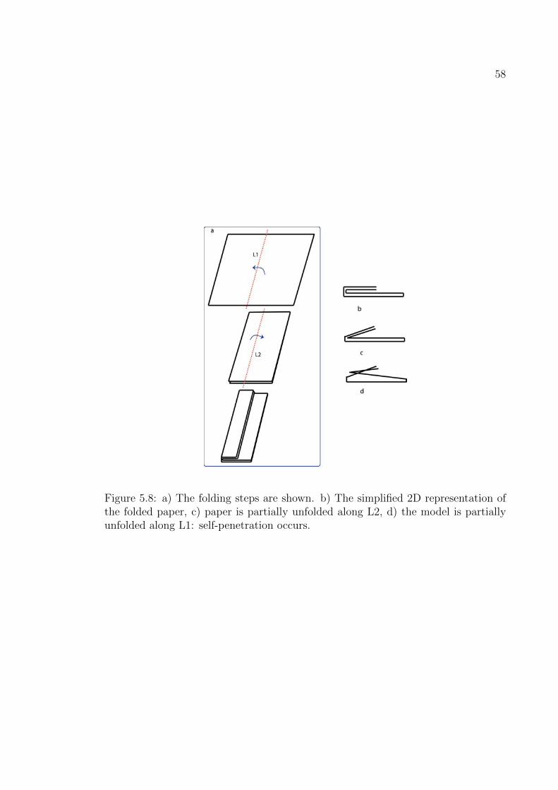
58

Figure 5.8: a) The folding steps are shown. b) The simplified 2D representation ofthe folded paper, c) paper is partially unfolded along L2, d) the model is partiallyunfolded along L1: self-penetration occurs.

59

Figure 5.9: Rendering coplanar faces with overlapping areas. Narrow strips are usedto separate two faces (a,b). (Images redrawn from [75])

may consist of several coplanar faces with overlapping areas (fig.5.7), which possibly

have different colors in the two sides of the paper (as it is very common in traditional

origami where they use colorful papers with different colors on different sides of the

paper). For partial foldings, the usual z-buffer method can be used to render the

model. However, assuming that the paper has no thickness, it is difficult to render

those faces that are located in the same plane. In particular, the usual z-buffer

method fails to deal with the problem of visualizing origami models that have some

faces located in the same plane since the depth value of overlapping pixels for these

faces is the same.

Thiel [75] addresses this problem by modifying the model and unfolding it a little,

making the origami “nearly flat”. This modification helps to understand the origami

configuration visually, however, this solution would be problematic since paper self-

penetrations might happen (fig.5.8), and z-buffer may produce invalid results near

the fold lines due to round-off errors. She discusses an alternative method, where

the two overlapping coplanar faces would be rendered parallel but slightly separated.

In this method, the fold lines would be rendered as a narrow strip (or set of narrow

strips for more realistic rendering) parallel to the fold line (fig.5.9a,b). However,

60

Figure 5.10: Miyazaki’s technique for face order renewal. Three predefined fold types(a-c) and the order of faces after folding. Bold lines represent the moving faces. In“a”, new face stacks will be created, while in “b” and “c” the existing stacks areupdated.(Images redrawn from [53])

this solution only works for single folds, and as new folds are introduced to the

model, it becomes more difficult to find the proper configuration for the faces and the

narrow strips. This method is difficult to be implemented in practical applications.

An alternative technique for properly visualizing coplanar polygons is to sort the

polygons (faces) in the order in which they should be sent to the output pipeline for

rendering. Miyazaki et al. [53] keep faces sorted based on their rendering orders in

a stack while the origami model is interactively created. In this technique, when the

model is folded along a new line, the face stack is updated based on three predefined

cases. The fold operation is one of these three types: a) a bend, b) a fold up (folding

up is a specific case of bending where the folding degree is 180 degrees), or c) a tuck-

in (fig.5.10). Knowing the order of overlapping faces, an appropriate depth offset can

61

Figure 5.11: Circular ordering of faces; A is above B, B is above C, C is above D,and D is above A.(Images from [28])

be added to each face based on its order so that the z-buffer can be used to render

these faces properly[6]. Since, in Miyazaki’s application, only three fold types are

only allowed, the faces would never overlap in a circular fashion (fig.5.11), and hence

a linear data structure is sufficient.

An image space technique was proposed by Furuta et al. [28], which solves the

rendering problem by defining a matrix which represents the rendering order between

every pair of faces, and a 2D array of face IDs. The matrix of rendering order, which

is called the OR matrix, is obtained from an application called ORIPA (ORIPA gets

the final crease pattern of the model as the input and then folds the model based on

the pattern, as explained in Chapter 2). When the number of faces in the model is

N, then the NxN OR matrix describes all the rendering orders, where each element

mij of the matrix is: a) U (upper): if Fi lies on the top of Fj, b) L (lower): if Fi lies

beneath Fj, or c) 0: if Fi and Fj do not overlap (fig.5.12).

The array of face IDs is a KxM 2D array (K and M are the height and the width

of the rendering area respectively), which stores the ID of the most above face in

each pixel. This array is built by running a standard scan-line algorithm, where the

62

Figure 5.12: a) A simple crease pattern, b) a side view of the folded paper, c) theOR matrix for this configuration.(Images from [52])

pixels of each face is scanned row-by-row. For each pixel, based on the OR matrix,

if the current scanned face is above the face stored in ID array, then the current face

ID is replaced. In case of partial foldings in the model, the depth value obtained

from the z-buffer is used to assign values to the face ID array. At the end, based

on the constructed face ID array and the corresponding color of each face in each

pixel, the origami model is rendered to the output. This method can also handle

the circular overlapping of faces since it stores rendering information for each pair

of faces separately in OR matrix [52].

Furuta’s image-space technique for rendering coplanar polygons requires a low

level implementation that directly works with the values of image pixels, which

makes it more complex. The run-time complexity is dependent on the number of

pixels in the image, as for each single face all the pixels that the face is projected

into should be processed, in addition to the required time to obtain the OR matrix,

which is done based on a brute-force algorithm. In Miyazaki’s technique there is a

chance of self-penetration since partial foldings are allowed in the system. KiriSim

63

is very similar to Miyazaki’s system in nature, where to handle the rendering issue I

propose an object-space method solving Miyzaki’s and Furuta’s techniques pitfalls.

The proposed rendering algorithm has two phases: phase A, responsible for sorting

the faces in the order in which they should be rendered (very similar to Miyazaki’s),

and phase B, dealing with the problem of rendering sorted coplanar faces, explained

in the following subsection.

5.4.1 A New Technique for Rendering Coplanar Faces in 3D Origami

Models

Phase A is very similar to Miyazaki’s method, where the order of faces is updated

in a set of predefined cases.The main difference of my technique and Miyzaki’s is in

phase B, where the visible parts of each polygon in each plane is determined and

rendered. Phase A and phase B of this method will be explained respectively.

Phase A

For rendering purposes, we need to know how the polygons are arranged in order in

each layer-set, which will be easy to accomplish if we keep the ordered list of facets for

each layer-set and update it according to the folding operations in the system and the

interactive object rotation. New layer-sets are generated when: a) a fold operation is

performed along a new fold line (fig.5.13a,b), or b) an unfolding operation along an

existing fold line is performed which results in affected faces with respect to that fold

line to be moved away from the fixed faces, and lie in a different plane (fig.5.13e,f).

In both cases “a” and “b”, new layer-sets are created along with their ordered face

lists, and other existing layer-sets face lists, if are involved in the operation, are

64

Figure 5.13: A folding operation is performed and a new layer-set is generated (a-b),view-transition occurs and layer-sets are updated (b-c), L1 and L2 are merged to asingle layer-set (d), view-transition occurs due to rotation and layer-set is updated(e), and unfolding operation is performed which results in separation of layer-sets(f).

65

Figure 5.14: Phase A of algorithm only sorts polygons locally in each layer-set. In thetop, the folding sequence is presented from left to right. Depending on the geometry(size of the polygons) we will end up in case a or b.

updated. Also, when two layer-sets lie on each other on the same plane as a result

of a folding operation along a fold line, they should be joined together, and their

faces lists should be merged (fig.5.13d). There is one other situation which requires

updating the face lists of the layer-sets as well, and it is when a view-transition

occurs (fig.5.13 transition from b to c, or transition from d to e). In the last case,

the order of the polygons in each layer-set which has gone through a view-transition

should be reversed.

Since we are starting from a single polygon, we can guarantee that the leaf poly-

gons in each layer-set are sorted locally1, but it does not sort all the polygons in the

model in different layer-sets globally. It is difficult to come up with an algorithm

that supports global depth sorting of polygons, since partial foldings may exist in

the model which results in having different layer-sets on different planes. Figure 5.14

illustrates that global depth sorting needs more complicated algorithms.

1By sorted locally we mean polygons are sorted within a single plane, and by sorted globally wemean they are sorted in the entire model with possibly polygons lying on different planes.

66

Figure 5.15: Basic idea of phase B. In blue rectangle the folding process is demon-strated. In the bottom, visible parts of each line segment (faces in 3D) are markedby “A”, “B”, and “C”.

Phase B

In phase A, all the leaf polygons (faces) were classified into the corresponding layer-

sets based on the plane each polygon lies in, where each layer-set has the sorted

list of its coplanar faces (based on the rendering orders between faces). Knowing

the order of faces in a particular plane, I proposed a new method for rendering the

coplanar polygons properly, explained below.

To illustrate this method, I have reduced the problem from 3D to 2D, where

faces are represented as 2D line segments, as dealing with line segments is easier for

visualizing and explanation purposes than dealing with polygons in 3D. The basic

idea is that in each layer-set, it is sufficient to only render the visible areas of each line

segment (leaf polygon or face in 3D). Those part of the line segments that are covered

by the line segments above them (are invisible) are not rendered. For instance, in

Figure 5.15, only part “C” of line segment “1”, part “B” of line segment “2”, and

67

part “A” of line segment “3” are visible from the point of view shown. Consequently,

each line segment (leaf polygons in 3D) should be partitioned into a set of smaller

line segments, where each smaller line segment can be specifically labeled either as

a visible line segment or as an invisible line segment.

There may be one or several layer-sets in a model (fig.5.13). In order to partition

the line segments into visible and invisible areas, the following steps should be ac-

complished for each layer-set separately (this procedure is illustrated in Figure 5.16

):

All the line segments (polygons in 3D) in a layer-set are given as the input. We

define a window in 2D as a line segment specified by its start-point and end-point.

S1 is a line passing from the window’s start-point, and S2 is a line passing from the

window’s end-point, where both S1 and S2 are perpendicular to the window. Let n

be the number of line segments, and k be the iteration number. Let R be the list

of the results of the algorithm containing all the visible and invisible line segments,

initialized to R = {l1} (fig.5.16).

Partitioning procedure:

a) Set the window’s start point and end point to the start point and end point

of l1, respectively. Set k to 1.

b) Split lk+1 by S1 and S2. Insert all the split line segments which do not lie

between the start-point and end-point of the window into R (those split line segments

that are not covered by the window are inserted into R).

c) Update the window by finding the two points “a” and “b” among all start-

point and end-point of line segments in R that have the maximum distance from each

other, and setting the window’s start point and end point to “a” and “b”. Update

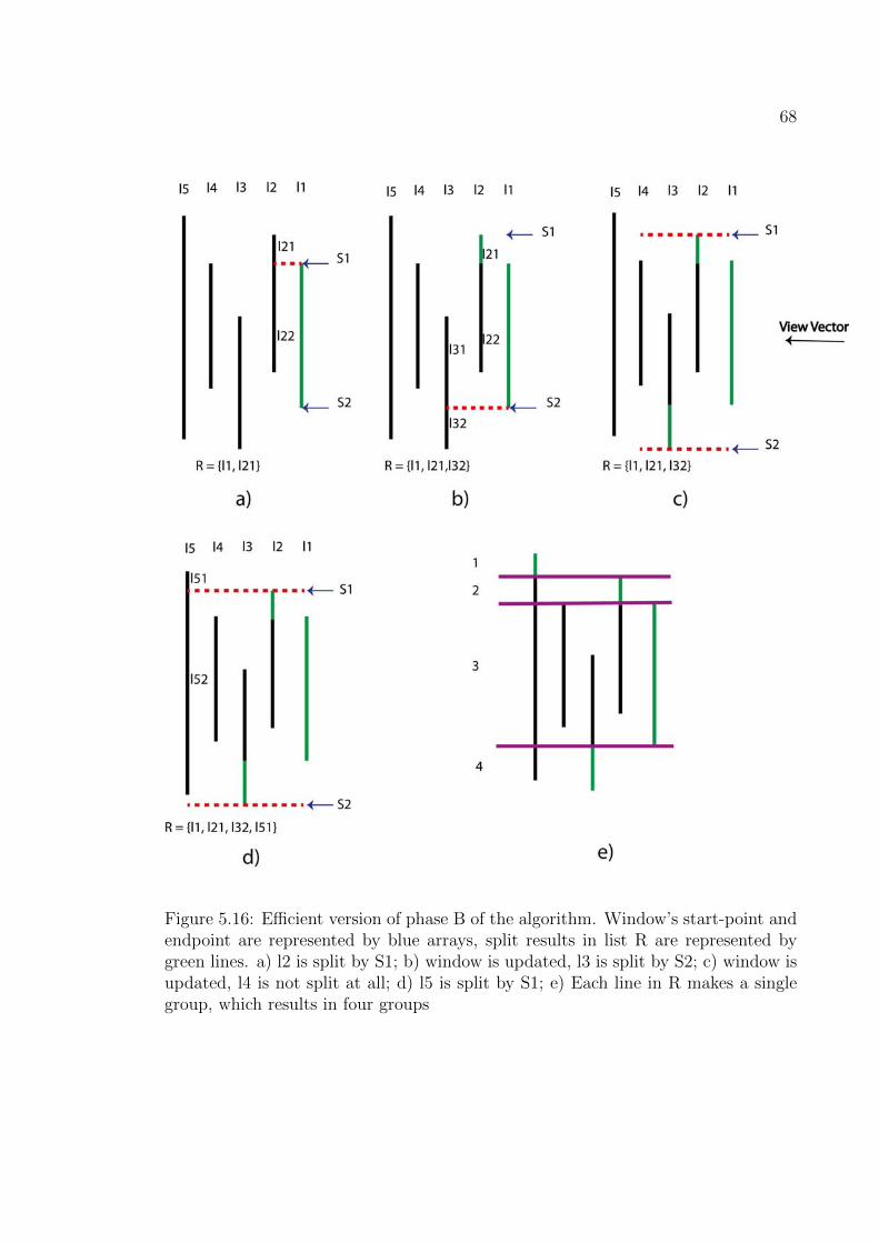
68

Figure 5.16: Efficient version of phase B of the algorithm. Window’s start-point andendpoint are represented by blue arrays, split results in list R are represented bygreen lines. a) l2 is split by S1; b) window is updated, l3 is split by S2; c) window isupdated, l4 is not split at all; d) l5 is split by S1; e) Each line in R makes a singlegroup, which results in four groups

69

S1 and S2. Increment k by 1, and go to step b if k is less than n.

At the end, it is sufficient to render the line segments in R, since they are the

only visible line segments in the model from the current view point.

The run-time complexity is O(n), since in each iteration we are only dealing with

one line segment. This algorithm can be extended to 3D for origami models, where

leaf polygons replace line segments. The window is generalized to a polygon, and

updating the window is performed by finding the union of the current window and

the polygon lk, in step k.

In this thesis, I have implemented a simpler version of this algorithm (simpler

from implementation perspective), which is as follows:

L, the list of all line segments: L = {l1, l2, ..., ln}, is given as the input to the

partitioning procedure, where n is the number of line segments in layer-set X. Let R

be the list of all the line segments which are the results of the procedure (the output

of the algorithm); initialized to R = {l1}, where l1 is the most above line segment in

X (l1 is completely visible in the layer-set from the current view point). Let SL be

the list of all the lines which are used to do partitioning procedure. SL is initialized

to s11 and s12, where sk1 is a line passing through lk’s start point, and sk2 is a line

passing through lk’s end point (fig.5.17), both perpendicular to it.

Partitioning procedure:

a) Set a variable k to 1.

b) Split lk+1 to ln by lines in SL and add the resulting line segments to the end of

the list R in order (e.g. in Figure 5.17, result line segments from l1, l2, l3, l4, l5 are

added to the list respectively).

c) If k + 1 is not equal to n, then list SL is updated to SL = {s(k+1)1, s(k+1)2};

70

Figure 5.17: Phase B of algorithm, n = 5: a) l2, l3, l5 are split by horizontal dashedlines. b) l3, l4, l5 are split by dashed lines. c) l4, l5 are split by dashed lines. d) l5is split by dashed lines. e)line segments are classified into groups 1-4.

71

increment k by 1; go to step b.

After partitioning all the line segments and storing the results in list R in order,

further processing on the results should be done to classify them into appropriate

“groups” for the final rendering. Each group consists of a set of overlapping line

segments (coplanar polygons in 3D) belonging to a specific layer-set in the simulated

folded model. Line segments in each group have either the same start-point and

end-point as the most above member of that group (in 3D, they have exactly the

same shape), or their start-point and end-point lie between the start-point and end-

point of the most above member (in 3D, they completely lie inside the area of the

most above member). In each group only the most above member is visible from the

current view point, and hence is rendered.

Let G be the list of groups in layer-set X. Let m be the size of list R = {r1, ..., rm},

the output of the partitioning procedure. The classification procedure to make groups

is done as follows:

Classification procedure:

a) Set a variable k to 1.

b) Remove rk from R. Make a group g with rk as its most above member (because

r1 to rm are in order from the previous procedure). Search through R and remove

all rq that are covered by rk from R (their start-point and end-point lie between the

start-point and end-point of rk), and add them to g.

c) Insert g to G. Increase k by 1; go to step b.

Now, each single group consists of a subset of line segments in R, where intersec-

tion of groups is empty. The most above member from each group should only be

rendered since it is visible to the viewer.

72

Figure 5.18: a) Best case, only one group results from phase B of algorithm; b) Worstcase, seven groups result from phase B of algorithm.

There are two cases in which phase B should be re-executed for all or some of

the layer-sets in the model: a) when the “view-transition” occurs, either by change

of the view point when the model is rotated, or when the model is folded/unfolded

along a particular fold line, and b) when two or more layer-sets should be joined

together or should be separated from each other.

The worst case time complexity is analyzed for the 2D version of phase B which

deals with line segments. In each step the maximum total number of line segments

in R is calculated, where n is the initial number of line segments:

step0 : n

step1 : 2(n− 1)

step2 : 4(n− 2)

step3 : 8(n− 3)

stepi : 2i(n− i)

Which means in total we have:

73

n∑i=0

2i(n− i) =n∑

i=0

n2i −n∑

i=0

i2i = n(2n+1 − 1)− (n− 1)2n+1 − 2 = 2n+1 − (n+ 2)

We can generalize this algorithm to 3D by replacing line segments with leaf polygons,

where l1 to ln are polygons in layer-set X, and SL = {s(k)1, s(k)2, ..., s(k)m} are all

edges of polygon lk in step k, and R is the list of all polygons which are the results

of partitioning procedure.

However, since the number of polygons in the models which are simulated by

KiriSim is about 1024 in average (having 10 folds in the model) and the computers

are so fast, we do not run into problems regarding the speed. The worst case and

the best case for phase B are shown in Figure 5.18.

Chapter 6

Implementation

In this chapter, the data structure which is designed for the development of KiriSim

is explained, and it is compared to some other existing data structures. Then, tools

and languages used for the development of this application are described.

6.1 Data Structure

In computer graphics, polygonal meshes are widely used to represent geometric mod-

els, and different data structures have been proposed for different applications and

goals. The data structure used to represent and manipulate a simulated sheet of pa-

per should be time efficient, because the virtual paper is manipulated interactively

and it is visualized in real time. Since partial foldings are allowed in the system, it

is important that the data structure is designed in a way that makes it easy for the

system to check for some of the illegal actions done by the user and prevent him/her

from them. For instance, stretching the paper is illegal and should be avoided.

Also, the data structure should maintain connectivity and overlapping relationships

between faces during the entire modeling and folding process.

Using a hierarchical data structure fits the nature of these applications (e.g.

KiriSim) well, as all the operations are performed in a sequence and each operation

is dependent on the previous operations. Furthermore, having a hierarchical history

of operations makes the implementation of undoing an operation easier and faster.

74

75

Also, it is better to avoid using triangular meshes, despite having some advantages

such as faster rendering by OpenGL as the vertices are passed more efficiently to the

hardware [71]. Because triangular meshes increase the complexity of the operations

as the number of polygons in the model will be increased. Some polygon mesh data

structures, such as half-edge [49], winged-edge [10], and vertex-vertex [72] structures

do not fulfill the requirements for the development of KiriSim. These representations

do not have the hierarchical structures, and they store some unnecessary additional

information (to make mesh traversal easier) which is not required in my application.

Additionally, dealing with a bunch of pointers to manipulate and access the data

structure is an error prone process, which in addition to more memory consumption,

it requires more work when a change is applied. In here, the nature of the problem

demands a specific data structure designed in a way that supports all defined oper-

ations in the system while maintaining its efficiency from both memory and speed

perspectives.

An object-oriented approach is used to design the data structure, where the

relationship between elements is indicated by a set of pointers. In the following sub-

section, first, a data structure used, previously, for similar applications is discussed,

and then the data structure which I have used in KiriSim is explained.

6.1.1 Data Structures Employed in Similar Applications

The common data structure used for modeling origami [42, 53, 54, 75, 70] is repre-

sented in Figure 6.1. The components of this data structure are: a) a binary tree

preserving the relationship between faces which are generated during the process of

folding, b) the operation list which keeps the overlapping relationship between copla-

76

Figure 6.1: Common data structure used in origami applications (the folding opera-tions and the crease pattern is shown in the top): a) hierarchy of faces, b) hierarchyof edges, c) list of operations with the ordered list of faces, d) vertex list (“C” in thevertex list represents the location of the vertex after each operation if it moves andthe initialization column shows which vertices initially existed in the model with Cas their initial location). Further explanation in the text.

77

nar faces, c) a binary tree structure which represents the relationship between edges

during the folding process, where some edges are divided into two smaller edges, and

d) a list of all vertices in the model with the history of their positions during different

folding operations (For instance, in Figure 6.1d, vertex V6 is generated by operation

1 and is moved by operation 2). Each face has pointers to its edges, and a pointer

to the operation during which it has been generated. Each edge has pointers to its

endpoint vertices and the face(s) it belongs to.

6.1.2 Data Structure Employed in KiriSim

A different data structure is used in KiriSim, where the main difference from the

one discussed in 6.1.1 is that edges are not considered as separate entities. Instead

of having edges in general (including non-crease edges, e.g. the boundaries of the

virtual paper), it is sufficient to, only, have creases and omit the overhead of storing

non-crease edges in the model as it is not necessary. In here, the model is represented

by a hierarchical face-vertex data structure, where faces have a list of their vertices

in clock-wise order. There are other entities in this data structure, such as creases

and layers, which are necessary for paper manipulation and rendering. Compared

to the other data structure, the amount of memory required to represent a model is

less, and we deal with smaller number of pointers which decreases the complexity,

and makes all operations faster and less error prone. Different parts of this data

structure are discussed below.

78

Figure 6.2: The employed data structure in KiriSim. a) the folding operations andthe crease pattern is shown, b) the corresponding hierarchical face-vertex structure,c) the layer-set for the current configuration, d) the fold-lines, their creases, and theaffected and produced faces with respect to each fold-line.

79

Faces

Each facet in the model is a convex polygon, where its edges are either boundaries

of the paper, or the crease segments. Facets are identified by a set of vertices, where

adjacent faces share vertices. Each face has a pointer to the fold line it has been

produced from, and a pointer to its parent. Furthermore, it keeps the list of 2D

texture coordinates mapping to its vertices. Figure 6.2b illustrates all existing faces

in the model and their hierarchical relationship.

Layer-Sets

Knowing the order of overlapping coplanar faces is necessary for rendering purposes

as explained in Chapter 5. For this purpose, for each set of coplanar overlapping

faces in the model, there is a corresponding “layer-set” which has a sorted list of faces

on that layer-set. It also has a list of all the visible polygons (the split polygons,

which are the result of the algorithm discussed in Chapter 5) on that layer-set which

should be rendered. For example, in Figure 6.2c, Layer-set1 has the ordered list of

faces (F4-F7), and a list of visible polygons (Q1-Q8).

Fold-Lines

When a user draws a new line segment on the screen to fold the paper along it,

a new “fold-line” object is created with the drawn line segment’s start point and

end point. Each fold-line has a list of “creases”, which have been introduced to the

crease pattern after performing the fold operation along that fold-line. For example,

in Figure 6.2d, AK and KE are L2’s corresponding creases in the crease pattern.

Each fold-line has a list of all polygons that are affected by this fold-line, which

saves the system from re-calculating affected polygons each time a folding/unfolding

80

operation is performed along that line (e.g. F7 and F5 are affected polygons with

respect to L2 in Figure 6.2d, and F4, F5, F6, F7 are produced polygons with respect

to L2). Also, a “type” variable shows if the fold line is a mountain fold (anticlinal)

or a valley fold (synclinal).

Other Elements

In addition to the discussed elements, some lists are employed in the system to keep

the record of all the actions the user has performed interactively. Based on these

records, models are saved into files and can be loaded later. Also, it is possible to

animate the entire modeling process, having saved the record of all actions during

the creation of the model.

6.2 Texture Mapping

In traditional origami the paper has usually textures with different colors on both

sides. To simulate a paper with different colors on both sides, I have used some

shading facilities in OpenGL, where by assigning different materials to the front and

the back of the polygons and enabling shading, different colors appear on the two

sides of the paper.

In KiriSim, the texture can be customized by the user, which is mapped to the

polygonal shapes existing in the model. The system performs affine texture map-

ping in association with the folding process, where texture coordinates are linearly

interpolated across the simulated paper.

81

6.3 Programming Language and Toolkits

This application has been developed under Linux (Ubuntu 11.10) using C++. OpenGL

library is employed for graphical representation, and Qt library was used to design

the interface. C++ is chosen for developing this application because it is fast and

efficient for an interactive application.

Chapter 7

Modeling with KiriSim

This chapter provides a description of how different leaf shapes and origami sculp-

tures can be modeled with KiriSim. In Section 7.1, the folding and cutting process

for modeling leaves is discussed, where the shape of the leaf can be varied by chang-

ing: a) the angles between the veins and anti-veins, b) the number of existing veins

(hence the number of folds in the model), c) the length and the position of the veins,

and d) the shape of the final cutting curve.

In Section 7.2, some origami and kirigami models simulated with KiriSim, and

their modeling processes are represented.

7.1 Modeling Leaf Shapes

In order to model a leaf shape, one should try to fold the simulated sheet of paper

in a manner similar to the way it is folded inside the bud. As discussed in Chapter

3, leaves are folded along the veins and anti-veins while growing inside the bud (if

they have secondary lobes, they are folded along the secondary veins as well). Based

on the type of the venation pattern in the leaf, different modeling steps should be

performed in KiriSim. Figure 7.1 shows three venation patterns that require different

modeling processes.

In here, the modeling processes for different palmate leaves with different vena-

tions types (cases “a”, “b”, and “c” in Figure 7.1) are discussed.

82

83

Figure 7.1: Different venations patterns require different modeling processes (mainveins are represented in red, anti-veins in blue). a) The petiole is located on one ofthe initial edges of the square sheet of paper. b) The petiole is located somewherein the middle area of the paper. c) Secondary veins exist in the leaf (it is possiblethat case b and c are combined in a leaf’s venation pattern).

Case “a”:

Start from the initial sheet of paper (fig.7.2a), and fold it along a line co-linear with

the mid-vein (fig.7.2b). Unfold the paper, and continue the folding process along

the anti-veins and veins in one half of the paper (fig.7.2c, d, e, f). Repeat the same

folding operations for the other half of the paper symmetrically. At the end, refold

the model along all the existing fold lines (fig.7.2g). Specify a b-spline curve as the

marginal cutting curve (fig.7.2h), and cut the model (fig.7.2i). Unfold the model

along all the fold lines to get the final shape of the leaf (fig.7.2j).

Case “b”:

Start from the initial sheet of paper, fold it along the mid-vein, and then perform

a straight cut operation passing through the petiole (fig.7.3a). Unfold the paper,

perform folding operations along the veins and anti-veins sequentially as in case “a”,

and then refold the paper along all the existing fold lines (fig.7.3b,c). Specify the

84

Figure 7.2: Modeling steps for a simple palmate leaf with no secondary lobes.

85

Figure 7.3: Modeling steps for a leaf in which petiole is located higher than thebottom edge of the initial square sheet of the paper.

marginal curve (fig.7.3c), and cut the paper (fig.7.3d). Unfold the paper to get the

leaf model (fig.7.3e).

Case “c”:

Start with the initial simulated sheet of paper, and fold it along the mid-vein

(fig.7.4a). Tear the paper along the mid-vein, starting from the petiole and ending

at the junction of the secondary vein with the mid-vein (fig7.4b). Then, fold the

paper along the secondary veins and secondary anti-veins to simulate the tucking

operation (fig.7.4c, d, e). Unfold the paper, and fold it along all the main veins and

86

Figure 7.4: Modeling steps for a palmate leaf with secondary lobes.

87

Figure 7.5: A maple leaf. The secondary lobes marked with circles can not becaptured by folding and cutting a paper. The red line (L1) is an anti-vein, which isnot co-linear with the bisector of the sinus (L2) (image from [15]).

anti-veins in both halves of the paper symmetrically (fig.7.4f). Refold the paper along

all the fold lines (fig.7.4g), specify the cutting curve, and cut the model (fig.7.4h, i).

Unfold the paper to get the final shape of the leaf with secondary lobes along the

mid-lobe (fig.7.4j).

7.1.1 Leaves Modeled with KiriSim

Some of the leaf shapes modeled with KiriSim are represented in Figure 7.6, 7.7,

7.8, 7.9, and 7.10. KiriSim is used to illustrate that leaves which are radially folded

(the folds are radiated from the petiole) can be modeled by folding and cutting a

sheet of paper, as Couturier et al. proposed. The models are very similar to the real

leaf shapes, however, there are several reasons that the shape (specially the margin)

slightly differs from the real leaf. In this modeling approach the three dimensionality

88

of the folded leaves is ignored since we are assuming the leaf is folded flat and

consequently it is collapsed into a simple 2D curve. To model leaves more accurately,

we should partially unfold them and replace the cutting curve with a cutting surface

(so that the three dimensionality of the bud is simulated). Additionally, veins and

anti-veins are not completely straight lines and they are curved form the petiole

to lobes and sinuses, while we are approximating them with straight lines. This

modeling technique is based on the assumption that the leaf margin is collapsed into

a simple curve, which can be cut along by a scissor, and consequently it requires the

anti-veins to be the bisector of sinuses and the veins to be the bisector of lobes (which

is not quite the case in some leaves. See Figure 7.5). Besides, leaves may expand

non-uniformly while they are being unfolded, which results in some asymmetries that

can not be captured by folding paper along straight lines and cutting it.

KiriSim can also be used to model secondary lobes with a combination of tearing

and folding operations. Modeling secondary lobes with KiriSim, I figured out that

there are a certain group of secondary lobes that can be modeled by folding and

cutting paper, and it includes those lobes that have an exact symmetric pair with

respect to the main vein they are located along. Otherwise geometric constraints in

rigid paper modeling does not allow us to fold the paper along the secondary lobes

that do not have a symmetric pair. For example, in Figure 7.5 the secondary lobes

marked with black circles can bot be captured by folding and cutting a paper.

89

Figure 7.6: Image and model of an Acer pseudoplatanus leaf, Sapindales, from leftto right in the top. Image and model of a Fatsiajaponica leaf, Apiales, from left toright in the bottom (images from [15])

90

Figure 7.7: Image and model of an Acer leaf, from left to right in the top. Imageand model of a Sweet gum leaf, from left to right in the bottom.

91

Figure 7.8: Image and model of a Ribes Nigrum leaf, Saxifragales, from left to rightin the top. Image and model of Acer pseudoplatanus leaf, Sapindales, from left toright in the bottom (images from [15]).

92

Figure 7.9: A maple leaf modeled with KiriSim. Secondary lobes are ignored in thetop, and secondary lobes are considered in the bottom (From left to right: the imageof the real leaf, the modeled leaf with a jungle green texture, image from [15]).

93

Figure 7.10: A maple leaf modeled with KiriSim. Secondary lobes are ignored in thetop, and secondary lobes are considered in the bottom (From left to right: the imageof the real leaf, the modeled leaf with a jungle green texture).

94

Figure 7.11: A bird modeled with KiriSim, and the corresponding modeling process(Mountain folds are represented in blue, valley folds in red, adding a new edgeoperation in yellow, and tearing in white). Further explanation in text.

95

7.2 Origami Modeling

In contrast to kirigami, origami only involves folding a paper to make a model (no

cutting or gluing is involved). However, most origami models include some complex

folding operations (such as prayer fold, see Chapter 2), which are difficult to be

simulated on an interactive computer application, specially when all the faces are

rigid. As explained in Chapter 4, I have introduced the tearing operation to have

more freedom on manipulating a paper which is simulated by a set of rigid faces.

For example, the modeling steps for making a bird in KiriSim is illustrated in Figure

7.11 to show how the tearing can be used to build more complicated models. First,

the simulated sheet of paper is folded along one of the diagonals (fig.7.11a). The

paper is unfolded, and one other folding operation is performed as shown in Figure

7.11b. Then, an edge is added to the model along the yellow line (fig.7.11c) to be

able to do the tearing operation (fig.7.11d). A sequence of folding operations are

performed (fig.7.11e,f), and then the previous operations are done symmetrically on

the other half of the paper (fig.7.11g). After doing two additional folding operations

(fig.7.11h,i), the model is unfolded, and we start to refolded the model along the

existing fold lines: in Figure 7.11j, the model is refolded along the fold lines created

in steps f and g, then the model is refolded along the fold line created in step h

(7.11k), and finally the refolding is performed along the initial diagonal fold line.

The same steps are performed for the other half, symmetrically (fig.7.11m), and

another folding operations is performed to create the head of the bird (fig.7.11n).

To illustrate the process of simulating a prayer fold, another example consisting

of a prayer fold is shown Figure 7.12. Some other origami models simulated with

96

Figure 7.12: An insect modeled with KiriSim which requires a prayer fold (a-c), andits corresponding modeling process.

KiriSim, along with their crease pattern are represented in Figure 7.13, 7.14, 7.15,

7.17.

97

Figure 7.13: A frog modeled with KiriSim (in the top right), a photo of the realmodel (in the top left), and the crease pattern (in the bottom).

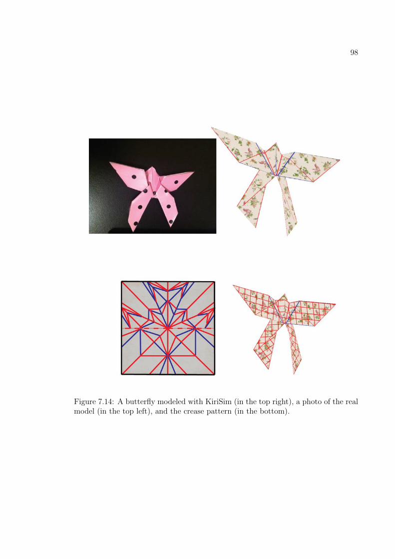
98

Figure 7.14: A butterfly modeled with KiriSim (in the top right), a photo of the realmodel (in the top left), and the crease pattern (in the bottom).

99

Figure 7.15: Simple origami models, which are made by a sequence of mountain andvalley folding operations (on the left), and the crease patterns (on the right).

100

Figure 7.16: A cup, a Samurai hat, and a heart modeled with KiriSim (on the right),and their crease patterns (on the left).

101

Figure 7.17: Origami models which only consist a sequence of mountain and val-ley folding operations, and a single tucking operation (on the left), and the creasepatterns (on the right).

102

Figure 7.18: A kirigami model simulated with KiriSim. a-f) folding the paper, whilein step “c” a straight cut operation along L, and in step “f” a final cutting curveoperation is performed. g) The final model with its crease pattern.

103

Figure 7.19: A kirigami model simulated with KiriSim. Folding the paper and cuttingit along the specified curve (in the top), and the final model (in the bottom).

104

Figure 7.20: A kirigami model simulated with KiriSim. a-d) Folding the paper, d)one “straight cut” operation followed by a final “cutting along curve” operation isperformed. e) The final model with crease pattern.

105

Figure 7.21: THE END. All the characters (T, H, E, N, D) are generated by KiriSim,based on “one straight cut” theory by Demaine [23].

Chapter 8

Conclusions

8.1 Summary of Contributions

In this thesis, I designed and developed an interactive program, called KiriSim, which

provides a modeling environment for folding and cutting a simulated sheet of paper.

The primary objective of KiriSim is to model leaf shapes based on the modeling

approach proposed by Couturier et al. [14]. They observed that the final shape of

the leaf is determined by the way it is folded along the veins and anti-veins within the

bud. Inspired by this observation, they proposed that a leaf shape can be modeled

by folding a sheet of paper and cutting it along the margin of the leaf using kirigami.

To model leaves with KiriSim, a simulated sheet of paper is folded along specific lines

(main veins and anti-veins), and the folded model is cut along a user-specified B-

spline curve (leaf’s margin). As well as the folds along the main veins and anti-veins,

it is possible to simulate the folds along the secondary veins by using an additional

operation (the tearing operation) in KiriSim. This way, the secondary lobes can also

be modeled with the system (the same method can be used to model tertiary lobes).

By means of KiriSim, I investigated Couturier’s modeling technique and found some

of its strong points and weak points. This modeling approach suits well for those leaf

types that are radially folded (all the folds start from the petiole), and the resulting

models are very similar to actual leaf shapes. However, there are some shortcomings

that arise due to a number of reasons. One of the most important reasons is that in

106

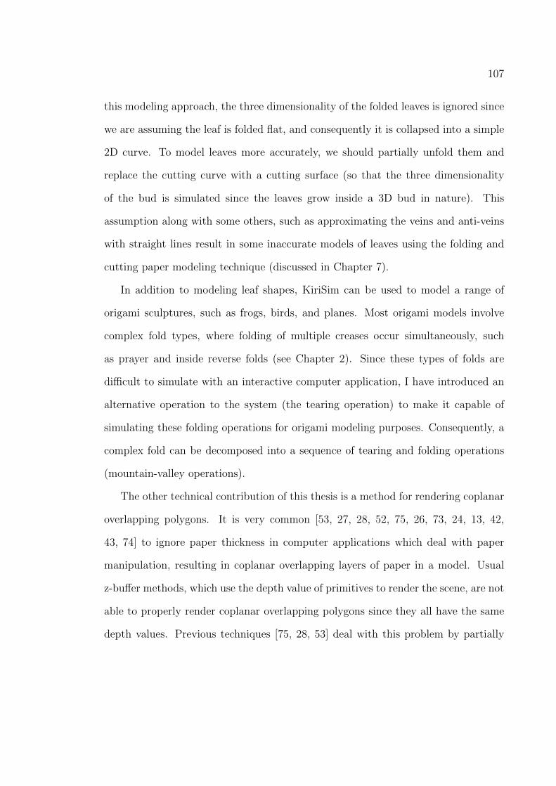
107

this modeling approach, the three dimensionality of the folded leaves is ignored since

we are assuming the leaf is folded flat, and consequently it is collapsed into a simple

2D curve. To model leaves more accurately, we should partially unfold them and

replace the cutting curve with a cutting surface (so that the three dimensionality

of the bud is simulated since the leaves grow inside a 3D bud in nature). This

assumption along with some others, such as approximating the veins and anti-veins

with straight lines result in some inaccurate models of leaves using the folding and

cutting paper modeling technique (discussed in Chapter 7).

In addition to modeling leaf shapes, KiriSim can be used to model a range of

origami sculptures, such as frogs, birds, and planes. Most origami models involve

complex fold types, where folding of multiple creases occur simultaneously, such

as prayer and inside reverse folds (see Chapter 2). Since these types of folds are

difficult to simulate with an interactive computer application, I have introduced an

alternative operation to the system (the tearing operation) to make it capable of

simulating these folding operations for origami modeling purposes. Consequently, a

complex fold can be decomposed into a sequence of tearing and folding operations

(mountain-valley operations).

The other technical contribution of this thesis is a method for rendering coplanar

overlapping polygons. It is very common [53, 27, 28, 52, 75, 26, 73, 24, 13, 42,

43, 74] to ignore paper thickness in computer applications which deal with paper

manipulation, resulting in coplanar overlapping layers of paper in a model. Usual

z-buffer methods, which use the depth value of primitives to render the scene, are not

able to properly render coplanar overlapping polygons since they all have the same

depth values. Previous techniques [75, 28, 53] deal with this problem by partially

108

unfolding the model, offsetting coplanar faces based on their rendering order, and

image space rendering. In contrast to these existing methods, I have proposed and

implemented a technique rooted in computational geometry to solve this rendering

issue. My algorithm keeps track of folding operations and rendering orders between

faces (which face lies in front of the other face and so on), then finds the portions

from each polygon that are visible to the viewer. This way, there is no need to

render all the polygons in a plane, and it is only sufficient to render all parts from

each polygon that are not covered by any other polygon.

8.2 Future Work

There is a number of problems which remain open for further research. These prob-

lems can be divided into two main categories: improving the application from the

perspective of a tool for manipulating paper to make artistic paper models (e.g.

origami and kirigami), and enhancing the system’s features and capabilities to model

more realistic leaf shapes.

8.2.1 Paper Manipulation Perspective

Some possible contributions are making more realistic animations of the paper while

it is folding/unfolding, introducing curved surfaces to the system to be able to create

a larger variety of paper models, and improving system’s interface. With the current

modeling approach, where all the faces are rigid, it is not possible to animate more

complex fold types such as “prayer fold” (introduced in Chapter 2, fig.2.2), as it

requires the paper to be bent. Physically-based approaches such as mass-spring

109

models may be one possible solution to animate these complex folding operations and

supporting curved surfaces, however, mass-spring modeling are not quite well-suited

to this problem. For instance, paper is not stretchable, and numerical problems arise

in mass-spring system in this case. A more general problem is that physically-based

approaches are slow compared to geometrical techniques [40].

Rendering realistic paper objects is an interesting area for future work. Visu-

alizing paper models requires advanced rendering techniques, where more realistic

lighting needs to be added to the 3D scene. In addition to the light which comes

directly from a light source, subsequent cases in which light rays from the same

source are reflected by other surfaces in the scene should also be taken into account.

Self-shadowing can improve the animation of paper folding/unfolding and make it

look a lot more realistic, while it is quite necessary for paper models which have

partial foldings in their configurations. The most interesting part would be render-

ing coplanar faces correctly (subsurface scattering and the Kubelka-Munk theory are

two possible techniques that can used for this purpose).

Another open area is to improve the system’s interface and user interaction with

the system. One possible improvement regarding user interface is to come up with a

better technique for selecting specific faces among all the overlapping coplanar faces,

which is quite a necessary feature for creation of many origami models. For example,

in KiriSim, if the user performs a folding operation, all the faces intersecting with

the fold line will be affected and folded, whether the user only wants some layers

to be affected or not, and this is not desirable (in Chapter 4, I have discussed the

solution provided for KiriSim).

The other possible future work would be extending this application to be usable

110

on tablets as these handy devices are becoming increasingly popular and the interface

on a tablet may also lend itself well to this problem. To my knowledge, there is only

one interactive application developed for making origami models on tablets, which

only has the features to do basic origami operations (mountain and valley folds) [13],

and it is not designed for modeling leaf shapes.

8.2.2 Modeling Leaf Shapes Perspective

KiriSim is well designed for modeling leaf shapes based on the method Couturier

[14] has proposed, however, the system’s interface can be improved by providing

some tools for doing some parts of modeling automatically (instead of asking the

user to do them all, interactively), or adding some features to the system to do

post-processing on the resulting leaf shapes. For example, as many leaves have self-

similar structures, and most are highly symmetric, adding some features which allow

the user to easily produce these symmetries and self-similarities during the modeling

process is quite desirable. Also, when leaves are unfolding, they start expanding non-

uniformly, which adds some asymmetries to their shape. Consequently, after cutting

the folded paper along the user-specified B-spline curve in KiriSim, and unfolding

the modeled leaf, it would be nice to have some tools for modifying the margin of the

leaf (e.g. adding asymmetric serrations along the margin). One possible technique

to implement this interface is to approximate the entire unfolded leaf margin by

another B-spline, and allowing the user to deform the margin by moving the control

points. In the same context, a similar idea can be employed to allow the user to

deform the leaf surface in 3D by approximating the surface with bi-cubic patches.

In nature, leaves’ have a thickness, and veins and buds are 3D volumes. In

111

this thesis, the leaf’s thickness has been ignored, and consequently, the bud has

been considered as a 2D envelope. To replace 2D envelopes with 3D volumes, the

cutting curve in current system should be replaced with a cutting surface as the

leaf is not folded flat anymore. Also, involving paper thickness in the simulation

adds complexities to the implementation, such as a need for more complicated data

structures. It is not easy to generalize the geometric representation of paper folding

to volumetric simulation, where faces and fold lines (creases) should be replaced by

appropriate volumes

From visualizing perspective, more effort can be put in the rendering area to get

more aesthetic models. For instance, normal maps or bump maps can be employed

to get better visualization of the leaves.

Bibliography

[1] Animal Workshop (origami). http://www.davidpetty.me.uk/

origamisoftware.htm.

[2] Flood fill algorithm. http://en.wikipedia.org/wiki/Floodfill.

[3] HyperGami. http://l3d.cs.colorado.edu/~ctg/projects/hypergami/

JavaGami.html.

[4] R. Lang. Origami. http://www.langorigami.com/science/origamisim/

origamisim.php4.

[5] R. Lang. Tree-Maker. http://www.langorigami.com/science/treemaker/

treemaker5.php4l.

[6] Rendering Coplanar Primitives in OpenGL. http://www.opengl.org/

resources/faq/technical/polygonoffset.html.

[7] T. Agui, M. Takeda, and M. Nakajima. Animating planar folds by computer.

Image Processing, pages 244–254, 1983.

[8] D. Balkcom. Robotic origami folding. Submitted in partial fulfillment of the

requirements for the degree of Doctor of Philosophy in Robotics, Carnegie Melon

University, Pittsburgh, Pennsylvania, 2004.

[9] D. Balkcom and M. Mason. Introducing robotic origami folding. In Proceedings

of IEEE International Conference on Robotics and Automation, 2004.

112

113

[10] B. Baumgart. A polygonhedron representation for computer vision. In AFIP-

SConference Proceedings (Proceedings of the National Computer Conference,

May1922, 1975. Anaheim, California), 44:589596, 1975.

[11] M. Bern, E. Demaine, D. Eppstein, and B. Hayes. A disk-packing algorithm

for an origami magic trick. In Proceedings of the 3rd International Meeting of

Origami Science, Math, and Education, Monterey, California, 2001.

[12] J. Bloomenthal. Modeling the mighty maple. In ACM SIGGRAPH Computer

Graphics, Proceedings of the 12th annual conference on Computer graphics and

interactive technique, 19, 1985.

[13] S. Chang, B. Stuart, and B. Wunsche. Origami simulator : a multi-touch

experience. In CHI 2009, ACM, pages 246–247, 2009.

[14] E. Couturier, E. Courrech du Pont, and S. Douady. A global regulation inducing

the shape of growing folded leaves. PLoS ONE, 4(11), 2009.

[15] E. Couturier, E. Courrech du Pont, and S. Douady. The filling law: a general

framework for leaf folding and its consequences on leaf shape diversity. Journal

of theoretical biology, 289C:47–64, August 2011.

[16] E. Demaine. Folding and unfolding. A thesis presented to the University of

Waterloo in fulfillment of the thesis requirement for the degree of Doctor of

Philosophy in Computer Science, 2001.

[17] E. Demaine, M. Demain, and A. Lubiw. Folding and cutting paper. Discrete

114

and Computational Geometry, Lecture Notes in Computer Science, 1763:104–

118, 2000.

[18] E. Demaine and M. Demaine. Recent results in computational origami. In

proceedings of the 3rd International Meeting of Origami, pages 1–10, 2001.

[19] E. Demaine and M. Demaine. Fold-and-cut magic. In Tribute to a Mathemagi-

cian, pages 23–30, 2004.

[20] E. Demaine, M. Demaine, A. Hawksley, H. Ito, P. Loh, Sh. Manber, and

O. Stephens. Making polygons by simple folds and one straight cut. In Revised

Papers from the China-Japan Joint Conference on Computational Geometry,

Graphs and Applications (CGGA 2010), Lecture Notes in Computer Science,

Dalian, China, pages 27–43, 2010.

[21] E. Demaine, M. Demaine, and A. Lubiw. Folding and one straight cut suffice.

in Revised Papers from the Japan Conference on Discrete and Computational

Geometry (JCDCG’98), Lecture Notes in Computer Science, 1763:104117, 1998.

[22] E. Demaine, M. Demaine, and A. Lubiw. Folding and one straight cut suffice. in

Proceedings of the 10th Annual ACM-SIAM Symposium on Discrete Algorithms

(SODA’99), Baltimore, Maryland, page 891892, 1999.

[23] E. Demaine and J. O’Rouke. Geometric folding algorithms: linkages, origami,

polyhedra. Cambridge University Press, 2007.

[24] J. Fastag. eGami: Virtual paperfolding and diagramming. The Fourth In-

ternational Conference on Origami in Science, Mathematics, and Education

115

(4OSME), 2006.

[25] J. Fastag. eGami: virtual paperfolding and diagramming software. Origami 4,

A K Peters/CRC Press, pages 273–283, 2009.

[26] D. Fisher. Origami on computer. http://origami.kvi.nl/articles/thesis.

ps.

[27] Y. Furuta, J. Mitani, and Y. Fukui. Modeling and animation of 3D origami

using spring-mass simulation. Science And Technology, 2008.

[28] Y. Furuta, J. Mitani, and Y. Fukui. A rendering method for 3D origami models

using face overlapping relations. Smart Graphics, 2009 - Springer, pages 193–

202, 2009.

[29] D. Goldberg. Genetic algorithms in search, optimization, and machine learning.

Addison-Wesley, page 432, 1989.

[30] M. Hammel, P. Prusinkiewicz, and B. Wyvill. Modeling compound leaves using

implicit contours. Proceedings of 10th international conference of the computer

graphics society on visual computing, 92(June):199–212, 1992.

[31] B. Hawkes, N. Benbernou, H. Tanaka, S. Kim, E. Demaine, D. Rus, and

R. Wood. Programmable matter by folding. Proceedings of the National

Academy of Sciences of the United States of America, 107:441–447.

[32] S. Hong, B. Simpson, and G. Baranoski. Interactive venation-based leaf shape

modeling. Natural phenomena and special effects. Comput. Animat. Virtual

Worlds, 16(3-4):415–427, July 2005.

116

[33] T. Hull. The combinatorics of flat folds : a survey. Proceedings of the 3rd

International Meeting on origami, 2002.

[34] T. Hull. Origami. Encyclopedia of the history of science, technology, and

medicine in non-western cultures, pages 1797–1800, 2008.

[35] T. Ida, M. Marin, and H. Takahashi. Constraint functional logic programming

for origami construction. Programming languages and systems Lecture Notes in

Computer Science, 2895:73–88, 2003.

[36] T. Ijiri and M. Yokoo. Surface-based growth simulation for opening flowers.

Proceedings of graphics interface, pages 227–234, 2008.

[37] W. Ju, L. Bonanni, R. Fletcher, R. Hurwitz, T. Judd, R. Post, M. Reynolds, and

J. Yoon. Origami desk. Proceedings of the conference on Designing interactive

systems processes, practices, methods, and techniques - DIS ’02, page 399, 2002.

[38] K. Kaino. Geometry of folded pattern of veins and origami model of digitate

leaves. Forma, pages 253–257, 1994.

[39] K. Kaino, K. Yajima, and N. Chiba. CG Image generation of flower arrange-

ment. Science, pages 207–212, 2000.

[40] Y. Kang and H. Cho. Interactive simulation of folded paper with breakable

hinge springs and fractal surface. The visual computer, 2004.

[41] A. Kasem and T. Ida. Computational origami environment on the web. Fron-

tiers of computer science in China, 2(1):39–54, 2008.

117

[42] J. Kato, T. Watanabe, H. Hase, and T. Nakayama. Understanding illustrations

of origami drill books. Information Processing Society of Japan, 41, 2000.

[43] N. Kishi and Y. Fujii. Origami , folding paper over the web. Proceedings of 3rd

Asia Pacific Computer Human Interaction, pages 337–3, 1998.

[44] H. Kobayashi, B. Kresling, and J. Vincent. The geometry of unfolding tree

leaves. Proceedings of the Royal Society B: Biological Sciences, 265(1391):147–

154, 1998.

[45] R. Lang. A computational algorithm for origami design. Proceeding SCG ’96

Proceedings of the twelfth annual symposium on Computational geometry, ACM

New York, NY, USA, 1996.

[46] R. Lang and T. Hull. Origami design secrets: mathematical methods for an

ancient art. Springer, 27(2):92–95, 2003.

[47] A. Lindenmayer. An introduction to parallel map generating systems. In

Proceedings of the 3rd International Workshop on Graph-Grammars and Their

Application to Computer Science, London, UK, 1987. Springer- Verlag, pages

27–40, 2010.

[48] Sh. Lu, Ch. Zhao, and X. Guo. Venation skeleton-based modeling plant leaf

wilting. International Journal of Computer Games Technology, pages 1–8, 2009.

[49] M. Mantyla. An introduction to solid modeling. Principles of Computer Sci-

ence Series. Computer Science Press, Rockville, Maryland, page 161174, 1988.

[50] H. Melichson. The art of paper cutting. Quarry books, 2011.

118

[51] J. Mitani. Recognition , modeling and rendering method for origami using 2D

bar codes. Proceedings of 4th International Conference on Origami, pages 2–2,

2006.

[52] J. Mitani. The folded shape restoration and the rendering method of origami

from the crease pattern. 13th International Conference on Geometry and Graph-

ics, 2008.

[53] Sh. Miyazaki. An origami playing simulator in the virtual space. Journal of

Visualization and Computer Animation, 7(March 1995):25–42, 1996.

[54] Sh. Miyazaki, T. Yasuda, and J. Toriwaki. An interactive simulation system for

origami based on virtual space manipulation. In Proceedings of IEEE Interna-

tional Workshop on Robot and Human Communication, 1992.

[55] L. Mundermann, P. Macmurchy, J. Pivovarov, and P. Prusinkiewicz. Modeling

lobed leaves. Computer Graphics International Conference, 2003.

[56] A. Peyrat, O. Terraz, S. Merillou, and E. Galin. Generating vast varieties of

realistic leaves with parametric 2Gmap L-systems. International Journal of

Computer Graphics archive, 24(7-9):807–816, June 2008.

[57] P. Prusinkiewicz. Modeling and visualization of biological structures. Graphics

interface, 1993, (May):128–137, 1993.

[58] P. Prusinkiewicz, M. Hammel, and E. Mjolsness. Animation of plant develop-

ment. SIGGRAPH 93 Proceedings of the 20th annual conference on Computer

119

graphics and interactive techniques. ACM New York, NY, USA, 93:351–360,

1993.

[59] P. Prusinkiewicz and A. Lindenmayer. Algorithmic beauty of plants. Springer-

Verlag, 1990.

[60] P. Prusinkiewicz and A. Runions. Computational models of plant development

and form. Review manuscript, pages 1–43, 2011.

[61] L. Quan, P. Tan, G. Zeng, and L. Yuan. Image-based plant modeling . In

Proceeding SIGGRAPH ’06 ACM SIGGRAPH 2006 Papers, ACM New York,

NY, USA, pages 599–604, 2006.

[62] J. Beatty R. Bartels and B. Barsky. An introduction to splines for use in

computer graphics and geometric modeling. Morgan Kaufman, Los Altos, Cal-

ifornia, 1987.

[63] Y. Rodkaew. Modeling leaf shapes using L-systems and genetic algorithms.

NICOGRAPH2002, pages 1–6, 2002.

[64] Y. Rodkaew and P. Chongstitvatana. Particle systems for plant modeling. In

Plant growth modeling and applications, Proceedings of PMA03. Tsinghua Uni-

versity Press and Springer, Beijing, pages 210–217, 2003.

[65] A. Runions. Modeling leaf form development. PhD Research Proposal, Univer-

sity of Calgary, pages 1–51.

[66] A. Runions. Modeling biological patterns using the space colonization algo-

rithm. A Thesis submitted to the faculty of graduate studies for degree of master

120

of science, page 74, oct 2008.

[67] A. Runions, M. Fuhrer, B. Lane, P. Federl, A. Rolland-Lagan, and

P Prusinkiewicz. Modeling and visualization of leaf venation patterns. ACM

Transactions on Graphics, 24(1), 2005.

[68] H. Scholten and A. Lindenmayer. A mathematical model for the laminar devel-

opment of simple leaves. Morphologie-Anatomie und Systematic der Pflanzen

5, page 2937, 1981.

[69] H. Scholten and A. Lindenmayer. A mathematical model for the laminar devel-

opment of simple leaves. In W. van Cotthem, editor, Morphologie-Anatomieund

Systematic der Pflanzen 5, pages 29–37, 1981.

[70] H. Shimanuki, J. Kato, and T. Watanabe. Recognition of folding process from

origami drill books. In Proceedings of Seventh International Conference on

Document Analysis and Recognition, 1(2):550–554, 2003.

[71] C. Smith. On vertex-vertex systems and their use in geometric and biological

modelling. A Thesis submitted to the faculty of graduate studies for degree of

doctor of philosophy, January 2006.

[72] C. Smith, P. Prusinkiewicz, and F. Samavati. Relational specification of subdi-

vision algorithms. Applications of Graph Transformations with Industrial Rel-

evance (AGTIVE 2003): Lecture Notes in Computer Science, 3062:313–327,

2003.

[73] T. Suzuki, J. Kato, and T. Watanabe. Extraction of contextual information

121

existing among component elements of origami books. Graphics Recognition

Algorithms and Applications, Lecture Notes in Computer Science, 2390:158–

166, 2002.

[74] T. Terashima, H. Shimanuki, J. Kato, and T. Watanabe. Interactive system for

origami creation. Interface, pages 182–194.

[75] J. Thiel. Interactive manipulation of virtual folded paper. A thesis submitted

in partial fulfillment of the requirements for the degree of master of science,

University of British Columbia, 1998.

[76] I. Wang, J. Wan, and G. Baranoski. Physically-based simulation of plant leaf

growth. Computer Animation and Virtual Worlds, 15(34):237–244, July 2004.