The TTEST Procedure - Worcester Polytechnic · PDF fileChapter 67 The TTEST Procedure Overview...

Chapter 67The TTEST Procedure

Chapter Table of Contents

OVERVIEW . . . . . . . . . . . . . . . . . . . . . . . . . . . . . . . . . . .3569

GETTING STARTED . . . . . . . . . . . . . . . . . . . . . . . . . . . . . .3570One-Samplet Test . . . . . . . . . . . . . . . . . . . . . . . . . . . . . . .3570Comparing Group Means . . . . . . . . . . . . . . . . . . . . . . . . . . . .3571

SYNTAX . . . . . . . . . . . . . . . . . . . . . . . . . . . . . . . . . . . . .3574PROC TTEST Statement .. . . . . . . . . . . . . . . . . . . . . . . . . . .3574BY Statement . . . . . . . . . . . . . . . . . . . . . . . . . . . . . . . . . .3575CLASS Statement . . . . . . . . . . . . . . . . . . . . . . . . . . . . . . . .3575FREQ Statement . . . . . . . . . . . . . . . . . . . . . . . . . . . . . . . .3576PAIRED Statement . . . . . . . . . . . . . . . . . . . . . . . . . . . . . . .3576VAR Statement . . . . . . . . . . . . . . . . . . . . . . . . . . . . . . . . .3577WEIGHT Statement . . . . . . . . . . . . . . . . . . . . . . . . . . . . . .3577

DETAILS . . . . . . . . . . . . . . . . . . . . . . . . . . . . . . . . . . . . .3577Input Data Set of Statistics. . . . . . . . . . . . . . . . . . . . . . . . . . .3577Missing Values . . . . . . . . . . . . . . . . . . . . . . . . . . . . . . . . .3577Computational Methods .. . . . . . . . . . . . . . . . . . . . . . . . . . .3578Displayed Output . . . . . . . . . . . . . . . . . . . . . . . . . . . . . . . .3582ODS Table Names . . . . . . . . . . . . . . . . . . . . . . . . . . . . . . .3583

EXAMPLES . . . . . . . . . . . . . . . . . . . . . . . . . . . . . . . . . . .3584Example 67.1 Comparing Group Means Using Input Data Set of Summary

Statistics . . . . . . . . . . . . . . . . . . . . . . . . . . . .3584Example 67.2 One-Sample Comparison Using the FREQ Statement . . . . .3587Example 67.3 Paired Comparisons . . . . . . . . . . . . . . . . . . . . . . .3588

REFERENCES . . . . . . . . . . . . . . . . . . . . . . . . . . . . . . . . . .3589

3568 � Chapter 67. The TTEST Procedure

SAS OnlineDoc: Version 8

Chapter 67The TTEST Procedure

Overview

The TTEST procedure performst tests for one sample, two samples, and paired ob-servations. The one-samplet test compares the mean of the sample to a given number.The two-samplet test compares the mean of the first sample minus the mean of thesecond sample to a given number. The paired observationst test compares the meanof the differences in the observations to a given number.

For one-sample tests, PROC TTEST computes the sample mean of the variable andcompares it with a given number. Paired comparisons use the one sample processon the differences between the observations. Paired comparisons can be made be-tween many pairs of variables with one call to PROC TTEST. For group comparisons,PROC TTEST computes sample means for each of two groups of observations andtests the hypothesis that the population means differ by a given amount. This latteranalysis can be considered a special case of a one-way analysis of variance with twolevels of classification.

The underlying assumption of thet test in all three cases is that the observations arerandom samples drawn from normally distributed populations. This assumption canbe checked using the UNIVARIATE procedure; if the normality assumptions for thettest are not satisfied, you should analyze your data using the NPAR1WAY procedure.The two populations of a group comparison must also be independent. If they are notindependent, you should question the validity of a paired comparison.

PROC TTEST computes the group comparisont statistic based on the assumptionthat the variances of the two groups are equal. It also computes an approximatet based on the assumption that the variances are unequal (the Behrens-Fisher prob-lem). The degrees of freedom and probability level are given for each; Satterthwaite’s(1946) approximation is used to compute the degrees of freedom associated with theapproximatet. In addition, you can request the Cochran and Cox (1950) approxima-tion of the

probability level for the approximatet. The folded form of theF statistic is computedto test for equality of the two variances (Steel and Torrie 1980).

FREQ and WEIGHT statements are available. Data can be input in the form of ob-servations or summary statistics. Summary statistics and their confidence intervals,and differences of means are output. For two-sample tests, the pooled-variance and atest for equality of variances are also produced.


Getting Started

One-Sample t Test

A one-samplet test can be used to compare a sample mean to a given value. Thisexample, taken from Huntsberger and Billingsley (1989, p. 290), tests whether themean length of a certain type of court case is 80 days using 20 randomly chosencases. The data are read by the following DATA step:

title ’One-Sample t Test’;data time;

input time @@;datalines;

43 90 84 87 116 95 86 99 93 92121 71 66 98 79 102 60 112 105 98;run;

The only variable in the data set,time, is assumed to be normally distributed. Thetrailing at signs (@@) indicate that there is more than one observation on a line. Thefollowing code invokes PROC TTEST for a one-samplet test:

proc ttest h0=80 alpha=0.1;var time;

run;

The VAR statement indicates that thetime variable is being studied, while the H0=option specifies that the mean of thetime variable should be compared to the value80 rather than the default null hypothesis of 0. This ALPHA= option requests 10%confidence intervals rather than the default 5% confidence intervals. The output isdisplayed in Figure 67.1.

One-Sample t Test

The TTEST Procedure

Statistics

Lower CL Upper CL Lower CL Upper CLVariable N Mean Mean Mean Std Dev Std Dev Std Dev Std Err Minimum Maximum

time 20 82.447 89.85 97.253 15.2 19.146 26.237 4.2811 43 121

T-Tests

Variable DF t Value Pr > |t|

time 19 2.30 0.0329

Figure 67.1. One-Sample t Test Results


Comparing Group Means � 3571

Summary statistics appear at the top of the output. The sample size (N), the mean andits confidence bounds (Lower CL Mean and Upper CL Mean), the standard deviationand its confidence bounds (Lower CL Std Dev and Upper CL Std Dev), and thestandard error are displayed with the minimum and maximum values of thetimevariable. The test statistic, the degrees of freedom, and thep-value for thet test aredisplayed next; at the 10%�-level, this test indicates that the mean length of the courtcases are significantly different from 80 days(t = 2:30; p = 0:0329).

Comparing Group Means

If you want to compare values obtained from two different groups, and if the groupsare independent of each other and the data are normally distributed in each group,then a groupt test can be used. Examples of such group comparisons include

� test scores for two third-grade classes, where one of the classes receives tutor-ing

� fuel efficiency readings of two automobile nameplates, where each nameplateuses the same fuel

� sunburn scores for two sunblock lotions, each applied to a different group ofpeople

� political attitude scores of males and females

In the following example, the golf scores for males and females in a physical educa-tion class are compared. The sample sizes from each population are equal, but this isnot required for further analysis. The data are read by the following statements:

title ’Comparing Group Means’;data scores;

input Gender $ Score @@;datalines;

f 75 f 76 f 80 f 77 f 80 f 77 f 73m 82 m 80 m 85 m 85 m 78 m 87 m 82;run;

The dollar sign ($) followingGender in the INPUT statement indicates thatGenderis a character variable. The trailing at signs (@@) enable the procedure to read morethan one observation per line.

You can use a groupt test to determine if the mean golf score for the men in the classdiffers significantly from the mean score for the women. If you also suspect that thedistributions of the golf scores of males and females have unequal variances, thensubmitting the following statements invokes PROC TTEST with options to deal withthe unequal variance case.



proc ttest cochran ci=equal umpu;class Gender;var Score;

run;

The CLASS statement contains the variable that distinguishes the groups being com-pared, and the VAR statement specifies the response variable to be used in calcula-tions. The COCHRAN option producesp-values for the unequal variance situationusing the Cochran and Cox(1950) approximation. Equal tailed and uniformly mostpowerful unbiased (UMPU) confidence intervals for� are requested by the CI= op-tion. Output from these statements is displayed in Figure 67.2 through Figure 67.4.


The TTEST Procedure

Statistics

UMPULower CL Upper CL Lower CL Lower CL

Variable Class N Mean Mean Mean Std Dev Std Dev Std Dev

Score f 7 74.504 76.857 79.211 1.6399 1.5634 2.5448Score m 7 79.804 82.714 85.625 2.028 1.9335 3.1472Score Diff (1-2) -9.19 -5.857 -2.524 2.0522 2.0019 2.8619

Statistics

UMPUUpper CL Upper CL

Variable Class Std Dev Std Dev Std Err Minimum Maximum

Score f 5.2219 5.6039 0.9619 73 80Score m 6.4579 6.9303 1.1895 78 87Score Diff (1-2) 4.5727 4.7242 1.5298

Figure 67.2. Simple Statistics

Simple statistics for the two populations being compared, as well as for the differenceof the means between the populations, are displayed in Figure 67.2. The Variable col-umn denotes the response variable, while the Class column indicates the populationcorresponding to the statistics in that row. The sample size (N) for each population,the sample means (Mean), and lower and upper confidence bounds for the means(Lower CL Mean and Upper CL Mean) are displayed next. The standard deviations(Std Dev) are displayed as well, with equal tailed confidence bounds in the LowerCL Std Dev and Upper CL Std Dev columns and UMPU confidence bounds in theUMPU Upper CL Std Dev and UMPU Lower CL Std Dev columns. In addition, stan-dard error of the mean and the minimum and maximum data values are displayed.


Comparing Group Means � 3573


The TTEST Procedure

T-Tests

Variable Method Variances DF t Value Pr > |t|

Score Pooled Equal 12 -3.83 0.0024Score Satterthwaite Unequal 11.5 -3.83 0.0026Score Cochran Unequal 6 -3.83 0.0087

Figure 67.3. t Tests

The test statistics, associated degrees of freedom, andp-values are displayed in Figure67.3. The Method column denotes whicht test is being used for that row, and theVariances column indicates what assumption about variances is being made. Thepooled test assumes that the two populations have equal variances and uses degreesof freedomn1+n2�2, wheren1 andn2 are the sample sizes for the two populations.The remaining two tests do not assume that the populations have equal variances. TheSatterthwaite test uses the Satterthwaite approximation for degrees of freedom, whilethe Cochran test uses the Cochran and Cox approximation for thep-value.


The TTEST Procedure

Equality of Variances

Variable Method Num DF Den DF F Value Pr > F

Score Folded F 6 6 1.53 0.6189

Figure 67.4. Tests of Equality of Variances

Examine the output in Figure 67.4 to determine whicht test is appropriate. The“Equality of Variances” test results show that the assumption of equal variances isreasonable for these data (the Folded F statisticF 0 = 1:53, with p = 0:6189). If theassumption of normality is also reasonable, the appropriate test is the usual pooledttest, which shows that the average golf scores for men and women are significantlydifferent (t = �3:83; p = 0:0024). If the assumption of equality of variances is notreasonable, then either the Satterthwaite or the Cochran test should be used.

The assumption of normality can be checked using PROC UNIVARIATE; if the as-sumption of normality is not reasonable, you should analyze the data with the non-parametric Wilcoxon Rank Sum test using PROC NPAR1WAY.



Syntax

The following statements are available in PROC TTEST.

PROC TTEST < options > ;CLASS variable ;PAIRED variables ;BY variables ;VAR variables ;FREQ variable ;WEIGHT variable ;

No statement can be used more than once. There is no restriction on the order of thestatements after the PROC statement.

PROC TTEST Statement

PROC TTEST < options > ;

The following options can appear in the PROC TTEST statement.

ALPHA= pspecifies that confidence intervals are to be100(1� p)% confidence intervals, where0 < p < 1. By default, PROC TTEST uses ALPHA=0.05. Ifp is 0 or less, or 1 ormore, an error message is printed.

CI=EQUALCI=UMPUCI=NONE

specifies whether a confidence interval is displayed for� and, if so, what kind. TheCI=EQUAL option specifies an equal tailed confidence interval, and it is the default.The CI=UMPU option specifies an interval based on the uniformly most powerfulunbiased test ofH0:� = �0. The CI=NONE option requests that no confidenceinterval be displayed for�. The values EQUAL and UMPU together request thatboth types of confidence intervals be displayed. If the value NONE is specified withone or both of the values EQUAL and UMPU, NONE takes precedence. For moreinformation, see the “Confidence Interval Estimation” section on page 3579.

COCHRANrequests the Cochran and Cox (1950) approximation of the probability level of theapproximatet statistic for the unequal variances situation.

DATA=SAS-data-setnames the SAS data set for the procedure to use. By default, PROC TTEST uses themost recently created SAS data set. The input data set can contain summary statisticsof the observations instead of the observations themselves. The number, mean, andstandard deviation of the observations are required for each BY group (one sampleand paired differences) or for each class within each BY group (two samples). For


CLASS Statement � 3575

more information on the DATA= option, see the “Input Data Set of Statistics” sectionon page 3577.

H0=mrequests tests againstm instead of 0 in all three situations (one-sample, two-sample,and paired observationt tests). By default, PROC TTEST uses H0=0.

BY Statement

BY variables ;

You can specify a BY statement with PROC TTEST to obtain separate analyses onobservations in groups defined by the BY variables. When a BY statement appears,the procedure expects the input data set to be sorted in order of the BY variables.

If your input data set is not sorted in ascending order, use one of the following alter-natives:

� Sort the data using the SORT procedure with a similar BY statement.

� Specify the BY statement option NOTSORTED or DESCENDING in the BYstatement for the TTEST procedure. The NOTSORTED option does not meanthat the data are unsorted but rather that the data are arranged in groups (ac-cording to values of the BY variables) and that these groups are not necessarilyin alphabetical or increasing numeric order.

� Create an index on the BY variables using the DATASETS procedure (in baseSAS software).

For more information on the BY statement, refer to the discussion inSAS LanguageReference: Concepts. For more information on the DATASETS procedure, refer totheSAS Procedures Guide.

CLASS Statement

CLASS variable ;

A CLASS statement giving the name of the classification (or grouping) variable mustaccompany the PROC TTEST statement in the two independent sample cases. Itshould be omitted for the one sample or paired comparison situations. If it is usedwithout the VAR statement, all numeric variables in the input data set (except thoseappearing in the CLASS, BY, FREQ, or WEIGHT statement) are included in theanalysis.

The class variable must have two, and only two, levels. PROC TTEST divides theobservations into the two groups for thet test using the levels of this variable. Youcan use either a numeric or a character variable in the CLASS statement.



Class levels are determined from the formatted values of the CLASS variable. Thus,you can use formats to define group levels. Refer to the discussions of the FOR-MAT procedure, the FORMAT statement, formats, and informats inSAS LanguageReference: Dictionary.

FREQ Statement

FREQ variable ;

Thevariable in the FREQ statement identifies a variable that contains the frequencyof occurrence of each observation. PROC TTEST treats each observation as if itappearsn times, wheren is the value of the FREQ variable for the observation. Ifthe value is not an integer, only the integer portion is used. If the frequency valueis less than 1 or is missing, the observation is not used in the analysis. When theFREQ statement is not specified, each observation is assigned a frequency of 1. TheFREQ statement cannot be used if the DATA= data set contains statistics instead ofthe original observations.

PAIRED Statement

PAIRED PairLists ;

The PairLists in the PAIRED statement identifies the variables to be compared inpaired comparisons. You can use one or morePairLists. Variables or lists of variablesare separated by an asterisk (*) or a colon (:). The asterisk requests comparisonsbetween each variable on the left with each variable on the right. The colon requestscomparisons between the first variable on the left and the first on the right, the secondon the left and the second on the right, and so forth. The number of variables on theleft must equal the number on the right when the colon is used. The differences arecalculated by taking the variable on the left minus the variable on the right for boththe asterisk and colon. A pair formed by a variable with itself is ignored. Use thePAIRED statement only for paired comparisons. The CLASS and VAR statementscannot be used with the PAIRED statement.

Examples of the use of the asterisk and the colon are shown in the following table.

These PAIRED statements... yield these comparisonsPAIRED A*B; A-B

PAIRED A*B C*D; A-B and C-D

PAIRED (A B)*(C D); A-C, A-D, B-C, and B-D

PAIRED (A B)*(C B); A-C, A-B, and B-C

PAIRED (A1-A2)*(B1-B2); A1-B1, A1-B2, A2-B1, and A2-B2

PAIRED (A1-A2):(B1-B2); A1-B1 and A2-B2


Missing Values � 3577

VAR Statement

VAR variables ;

The VAR statement names the variables to be used in the analyses. One-samplecomparisons are conducted when the VAR statement is used without the CLASSstatement, while group comparisons are conducted when the VAR statement is usedwith a CLASS statement. If the VAR statement is omitted, all numeric variables inthe input data set (except a numeric variable appearing in the BY, CLASS, FREQ, orWEIGHT statement) are included in the analysis. The VAR statement can be usedwith one- and two-samplet tests and cannot be used with the PAIRED statement.

WEIGHT Statement

WEIGHT variable ;

The WEIGHT statement weights each observation in the input data set by the valueof the WEIGHT variable. The values of the WEIGHT variable can be nonintegral,and they are not truncated. Observations with negative, zero, or missing values for theWEIGHT variable are not used in the analyses. Each observation is assigned a weightof 1 when the WEIGHT statement is not used. The WEIGHT statement cannot beused with an input data set of summary statistics.

Details

Input Data Set of Statistics

PROC TTEST accepts data containing either observation values or summary statis-tics. It assumes that the DATA= data set contains statistics if it contains a charac-ter variable with name–TYPE– or –STAT– . The TTEST procedure expects thischaracter variable to contain the names of statistics. If both–TYPE– and–STAT–variables exist and are of type character, PROC TTEST expects–TYPE– to containthe names of statistics including ‘N’, ‘MEAN’, and ‘STD’ for each BY group (orfor each class within each BY group for two-samplet tests). If no ‘N’, ‘MEAN’, or‘STD’ statistics exist, an error message is printed.

FREQ, WEIGHT, and PAIRED statements cannot be used with input data sets ofstatistics. BY, CLASS, and VAR statements are the same regardless of data set type.For paired comparisons, see the–DIF– values for the–TYPE–=T observations inoutput produced by the OUTSTATS= option in the PROC COMPARE statement (re-fer to theSAS Procedures Guide).

Missing Values

An observation is omitted from the calculations if it has a missing value for eitherthe CLASS variable, a PAIRED variable, or the variable to be tested. If more than



one variable is listed in the VAR statement, a missing value in one variable does noteliminate the observation from the analysis of other nonmissing variables.

Computational Methods

The t StatisticThe form of thet statistic used varies with the type of test being performed.

� To compare an individual mean with a sample of sizen to a valuem, use

t =�x�m

s=pn

where�x is the sample mean of the observations ands2 is the sample varianceof the observations.

� To comparen paired differences to a valuem, use

t =�d�m

sd=pn

where �d is the sample mean of the paired differences ands2d is the samplevariance of the paired differences.

� To compare means from two independent samples withn1 andn2 observationsto a valuem, use

t =(�x1 � �x2)�m

s

r1

n1+

1

n2

wheres2 is the pooled variance

s2 =(n1 � 1)s21 + (n2 � 1)s22

n1 + n2 � 2

ands21 ands22 are the sample variances of the two groups. The use of thiststatistic depends on the assumption that�21 = �22 , where�21 and�22 are thepopulation variances of the two groups.

The Folded Form F StatisticThe folded form of theF statistic,F 0, tests the hypothesis that the variances areequal, where

F 0 =max(s21; s

22)

min(s21; s2

2)


Computational Methods � 3579

A test ofF 0 is a two-tailedF test because you do not specify which variance youexpect to be larger. Thep-value gives the probability of a greaterF value under thenull hypothesis that�21 = �22 .

The Approximate t StatisticUnder the assumption of unequal variances, the approximatet statistic is computedas

t0 =�x1 � �x2pw1 + w2

where

w1 =s21n1; w2 =

s22n2

The Cochran and Cox ApproximationThe Cochran and Cox (1950) approximation of the probability level of the approxi-matet statistic is the value ofp such that

t0 =w1t1 +w2t2w1 +w2

wheret1 andt2 are the critical values of thet distribution corresponding to a signifi-cance level ofp and sample sizes ofn1 andn2, respectively. The number of degreesof freedom is undefined whenn1 6= n2. In general, the Cochran and Cox test tendsto be conservative (Lee and Gurland 1975).

Satterthwaite’s ApproximationThe formula for Satterthwaite’s (1946) approximation for the degrees of freedom forthe approximatet statistic is:

df =(w1 + w2)

2�w21

n1 � 1+

w22

n2 � 1

�

Refer to Steel and Torrie (1980) or Freund, Littell, and Spector (1986) for more in-formation.

Confidence Interval EstimationThe form of the confidence interval varies with the statistic for which it is computed.In the following confidence intervals involving means,t1��

2;n�1 is the100(1� �

2)%

quantile of thet distribution withn� 1 degrees of freedom. The confidence intervalfor

� an individual mean from a sample of sizen compared to a valuem is given by

(�x�m)� t1��

2;n�1

spn

where�x is the sample mean of the observations ands2 is the sample varianceof the observations



� paired differences with a sample of sizen differences compared to a valuemis given by

( �d�m)� t1��

2;n�1

sdpn

where �d ands2d are the sample mean and sample variance of the paired differ-ences, respectively

� the difference of two means from independent samples withn1 andn2 obser-vations compared to a valuem is given by

((�x1 � �x2)�m)� t1��

2;n1+n2�2s

r1

n1+

1

n2

wheres2 is the pooled variance

s2 =(n1 � 1)s21 + (n2 � 1)s22

n1 + n2 � 2

and wheres21 ands22 are the sample variances of the two groups. The use ofthis confidence interval depends on the assumption that�21 = �22 , where�21 and�22 are the population variances of the two groups.

The distribution of the estimated standard deviation of a mean is not symmetric, soalternative methods of estimating confidence intervals are possible. PROC TTESTcomputes two estimates. For both methods, the data are assumed to have a normaldistribution with mean� and variance�2, both unknown. The methods are as follows:

� The default method, an equal-tails confidence interval, puts an equal amountof area (�

2) in each tail of the chi-square distribution. An equal tails test of

H0:� = �0 has acceptance region

��2�

2;n�1 �

(n� 1)S2

�20

� �21��2

;n�1

�

which can be algebraically manipulated to give the following100(1 � �)%confidence interval for�2:

(n� 1)S2

�21�

�

2;n�1

;(n� 1)S2

�2�2;n�1

!

In order to obtain a confidence interval for�, the square root of each side istaken, leading to the following100(1 � �)% confidence interval:

s(n� 1)S2

�21�

�

2;n�1

;

s(n� 1)S2

�2�2;n�1

!


Computational Methods � 3581

� The second method yields a confidence interval derived from the uniformlymost powerful unbiased test ofH0:� = �0 (Lehmann 1986). This test hasacceptance region

�c1 � (n� 1)S2

�20

� c2

�

where the critical valuesc1 andc2 satisfy

Z c2

c1

fn(y)dy = 1� �

and Z c2

c1

yfn(y)dy = n(1� �)

wherefn(y) is the chi-squared distribution withn degrees of freedom. Thisacceptance region can be algebraically manipulated to arrive at

P

�(n� 1)S2

c2� �2 � (n� 1)S2

c1

�= 1� �

wherec1 and c2 solve the preceding two integrals. To find the area in eachtail of the chi-square distribution to which these two critical values correspond,solvec1 = �21��2;n�1

andc2 = �2�1;n�1 for �1 and�2; the resulting�1 and�2 sum to�. Hence, a100(1 � �)% confidence interval for�2 is given by

(n� 1)S2

�21��2;n�1

;(n� 1)S2

�2�1;n�1

!

In order to obtain a100(1 � �)% confidence interval for�, the square root istaken of both terms, yielding

s(n� 1)S2

�21��2;n�1

;

s(n� 1)S2

�2�1;n�1

!



Displayed Output

For each variable in the analysis, the TTEST procedure displays the following sum-mary statistics for each group:

� the name of the dependent variable

� the levels of the classification variable

� N, the number of nonmissing values

� Lower CL Mean, the lower confidence bound for the mean

� the Mean or average

� Upper CL Mean, the upper confidence bound for the mean

� Lower CL Std Dev, the lower confidence bound for the standard deviation

� Std Dev, the standard deviation

� Upper CL Std Dev, the upper confidence bound for the standard deviation

� Std Err, the standard error of the mean

� the Minimum value, if the line size allows

� the Maximum value, if the line size allows

� upper and lower UMPU confidence bounds for the standard deviation, dis-played if the CI=UMPU option is specified in the PROC TTEST statement

Next, the results of severalt tests are given. For one-sample and paired observationst tests, the TTEST procedure displays

� t Value, thet statistic for testing the null hypothesis that the mean of the groupis zero

� DF, the degrees of freedom

� Pr > |t|, the probability of a greater absolute value oft under the null hypothesis.This is the two-tailed significance probability. For a one-tailed test, halve thisprobability.

For two-samplet tests, the TTEST procedure displays all the items in the followinglist. You need to decide whether equal or unequal variances are appropriate for yourdata.

� Under the assumption of unequal variances, the TTEST procedure displaysresults using Satterthwaite’s method. If the COCHRAN option is specified, theresults for the Cochran and Cox approximation are also displayed.

� t Value, an approximatet statistic for testing the null hypothesis that themeans of the two groups are equal

� DF, the approximate degrees of freedom

� Pr > |t|, the probability of a greater absolute value oft under the nullhypothesis. This is the two-tailed significance probability. For a one-tailed test, halve this probability.


ODS Table Names � 3583

� Under the assumption of equal variances, the TTEST procedure displays resultsobtained by pooling the group variances.

� t Value, thet statistic for testing the null hypothesis that the means of thetwo groups are equal

� DF, the degrees of freedom

� Pr > |t|, the probability of a greater absolute value oft under the nullhypothesis. This is the two-tailed significance probability. For a one-tailed test, halve this probability.

� PROC TTEST then gives the results of the test of equality of variances:

� theF 0 (folded) statistic (see the “The Folded Form F Statistic” section onpage 3578)

� Num DF and Den DF, the numerator and denominator degrees of freedomin each group

� Pr > F, the probability of a greaterF 0 value. This is the two-tailed signif-icance probability.

ODS Table Names

PROC TTEST assigns a name to each table it creates. You can use these names toreference the table when using the Output Delivery System (ODS) to select tablesand create output data sets. These names are listed in the following table. For moreinformation on ODS, see Chapter 15, “Using the Output Delivery System.”

Table 67.1. ODS Tables Produced in PROC TTEST

ODS Table Name Description StatementEquality Tests for equality of variance CLASS statementStatistics Univariate summary statistics by defaultTTests t-tests by default



Examples

Example 67.1. Comparing Group Means Using Input Data Setof Summary Statistics

The following example, taken from Huntsberger and Billingsley (1989), comparestwo grazing methods using 32 steer. Half of the steer are allowed to graze continu-ously while the other half are subjected to controlled grazing time. The researcherswant to know if these two grazing methods impact weight gain differently. The dataare read by the following DATA step.

title ’Group Comparison Using Input Data Set of SummaryStatistics’;

data graze;length GrazeType $ 10;input GrazeType $ WtGain @@;datalines;

controlled 45 controlled 62controlled 96 controlled 128controlled 120 controlled 99controlled 28 controlled 50controlled 109 controlled 115controlled 39 controlled 96controlled 87 controlled 100controlled 76 controlled 80continuous 94 continuous 12continuous 26 continuous 89continuous 88 continuous 96continuous 85 continuous 130continuous 75 continuous 54continuous 112 continuous 69continuous 104 continuous 95continuous 53 continuous 21;run;

The variableGrazeType denotes the grazing method: ‘controlled’ is controlled graz-ing and ‘continuous’ is continuous grazing. The dollar sign ($) followingGrazeTypemakes it a character variable, and the trailing at signs (@@) tell the procedure thatthere is more than one observation per line. The MEANS procedure is invoked tocreate a data set of summary statistics with the following statements:

proc sort;by GrazeType;

proc means data=graze noprint;var WtGain;by GrazeType;output out=newgraze;

run;


Example 67.1. Using Input Data Set of Summary Statistics � 3585

The NOPRINT option eliminates all output from the MEANS procedure. The VARstatement tells PROC MEANS to compute summary statistics for theWtGain vari-able, and the BY statement requests a separate set of summary statistics for each levelof GrazeType. The OUTPUT OUT= statement tells PROC MEANS to put the sum-mary statistics into a data set callednewgraze so that it may be used in subsequentprocedures. This new data set is displayed in Output 67.1.1 by using PROC PRINTas follows:

proc print data=newgraze;run;

The–STAT– variable contains the names of the statistics, and theGrazeType vari-able indicates which group the statistic is from.

Output 67.1.1. Output Data Set of Summary Statistics

Group Comparison Using Input Data Set of Summary Statistics

Obs GrazeType _TYPE_ _FREQ_ _STAT_ WtGain

1 continuous 0 16 N 16.0002 continuous 0 16 MIN 12.0003 continuous 0 16 MAX 130.0004 continuous 0 16 MEAN 75.1885 continuous 0 16 STD 33.8126 controlled 0 16 N 16.0007 controlled 0 16 MIN 28.0008 controlled 0 16 MAX 128.0009 controlled 0 16 MEAN 83.125

10 controlled 0 16 STD 30.535

The following code invokes PROC TTEST using thenewgraze data set, as denotedby the DATA= option.

proc ttest data=newgraze;class GrazeType;var WtGain;

run;

The CLASS statement contains the variable that distinguishes between the groupsbeing compared, in this caseGrazeType. The summary statistics and confidenceintervals are displayed first, as shown in Output 67.1.2.



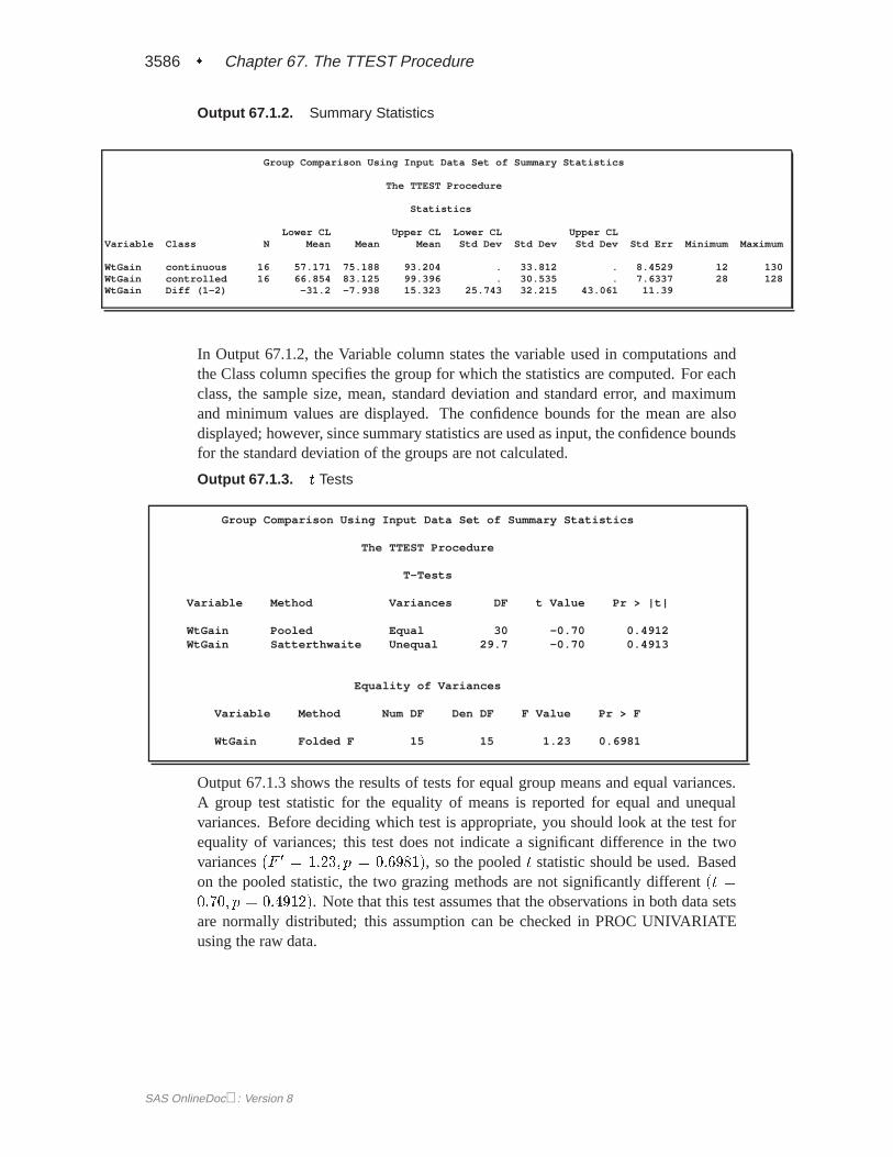
Output 67.1.2. Summary Statistics


The TTEST Procedure

Statistics

Lower CL Upper CL Lower CL Upper CLVariable Class N Mean Mean Mean Std Dev Std Dev Std Dev Std Err Minimum Maximum

WtGain continuous 16 57.171 75.188 93.204 . 33.812 . 8.4529 12 130WtGain controlled 16 66.854 83.125 99.396 . 30.535 . 7.6337 28 128WtGain Diff (1-2) -31.2 -7.938 15.323 25.743 32.215 43.061 11.39

In Output 67.1.2, the Variable column states the variable used in computations andthe Class column specifies the group for which the statistics are computed. For eachclass, the sample size, mean, standard deviation and standard error, and maximumand minimum values are displayed. The confidence bounds for the mean are alsodisplayed; however, since summary statistics are used as input, the confidence boundsfor the standard deviation of the groups are not calculated.

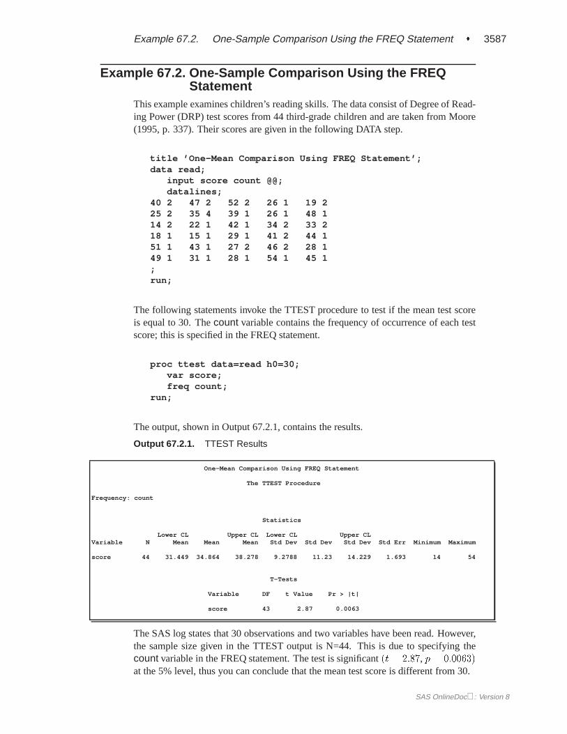
Output 67.1.3. t Tests


The TTEST Procedure

T-Tests

Variable Method Variances DF t Value Pr > |t|

WtGain Pooled Equal 30 -0.70 0.4912WtGain Satterthwaite Unequal 29.7 -0.70 0.4913

Equality of Variances

Variable Method Num DF Den DF F Value Pr > F

WtGain Folded F 15 15 1.23 0.6981

Output 67.1.3 shows the results of tests for equal group means and equal variances.A group test statistic for the equality of means is reported for equal and unequalvariances. Before deciding which test is appropriate, you should look at the test forequality of variances; this test does not indicate a significant difference in the twovariances(F 0 = 1:23; p = 0:6981), so the pooledt statistic should be used. Basedon the pooled statistic, the two grazing methods are not significantly different(t =0:70; p = 0:4912). Note that this test assumes that the observations in both data setsare normally distributed; this assumption can be checked in PROC UNIVARIATEusing the raw data.


Example 67.2. One-Sample Comparison Using the FREQ Statement � 3587

Example 67.2. One-Sample Comparison Using the FREQStatement

This example examines children’s reading skills. The data consist of Degree of Read-ing Power (DRP) test scores from 44 third-grade children and are taken from Moore(1995, p. 337). Their scores are given in the following DATA step.

title ’One-Mean Comparison Using FREQ Statement’;data read;

input score count @@;datalines;

40 2 47 2 52 2 26 1 19 225 2 35 4 39 1 26 1 48 114 2 22 1 42 1 34 2 33 218 1 15 1 29 1 41 2 44 151 1 43 1 27 2 46 2 28 149 1 31 1 28 1 54 1 45 1;run;

The following statements invoke the TTEST procedure to test if the mean test scoreis equal to 30. Thecount variable contains the frequency of occurrence of each testscore; this is specified in the FREQ statement.

proc ttest data=read h0=30;var score;freq count;

run;

The output, shown in Output 67.2.1, contains the results.

Output 67.2.1. TTEST Results

One-Mean Comparison Using FREQ Statement

The TTEST Procedure

Frequency: count

Statistics

Lower CL Upper CL Lower CL Upper CLVariable N Mean Mean Mean Std Dev Std Dev Std Dev Std Err Minimum Maximum

score 44 31.449 34.864 38.278 9.2788 11.23 14.229 1.693 14 54

T-Tests

Variable DF t Value Pr > |t|

score 43 2.87 0.0063

The SAS log states that 30 observations and two variables have been read. However,the sample size given in the TTEST output is N=44. This is due to specifying thecount variable in the FREQ statement. The test is significant(t = 2:87, p = 0:0063)at the 5% level, thus you can conclude that the mean test score is different from 30.



Example 67.3. Paired Comparisons

When it is not feasible to assume that two groups of data are independent, and anatural pairing of the data exists, it is advantageous to use an analysis that takes thecorrelation into account. Utilizing this correlation results in higher power to detectexisting differences between the means. The differences between paired observationsare assumed to be normally distributed. Some examples of this natural pairing are

� pre- and post-test scores for a student receiving tutoring

� fuel efficiency readings of two fuel types observed on the same automobile

� sunburn scores for two sunblock lotions, one applied to the individual’s rightarm, one to the left arm

� political attitude scores of husbands and wives

In this example, taken fromSUGI Supplemental Library User’s Guide, Version 5 Edi-tion, a stimulus is being examined to determine its effect on systolic blood pressure.Twelve men participate in the study. Their systolic blood pressure is measured bothbefore and after the stimulus is applied. The following statements input the data:

title ’Paired Comparison’;data pressure;

input SBPbefore SBPafter @@;datalines;

120 128 124 131 130 131 118 127140 132 128 125 140 141 135 137126 118 130 132 126 129 127 135;run;

The variablesSBPbefore andSBPafter denote the systolic blood pressure beforeand after the stimulus, respectively.

The statements to perform the test follow.

proc ttest;paired SBPbefore*SBPafter;

run;

The PAIRED statement is used to test whether the mean change in systolic bloodpressure is significantly different from zero. The output is displayed in Output 67.3.1.


References � 3589

Output 67.3.1. TTEST Results

Paired Comparison

The TTEST Procedure

Statistics

Lower CL Upper CL Lower CL Upper CLDifference N Mean Mean Mean Std Dev Std Dev Std Dev Std Err Minimum Maximum

SBPbefore - SBPafter 12 -5.536 -1.833 1.8698 4.1288 5.8284 9.8958 1.6825 -9 8

T-Tests

Difference DF t Value Pr > |t|

SBPbefore - SBPafter 11 -1.09 0.2992

The variablesSBPbefore andSBPafter are the paired variables with a sample sizeof 12. The summary statistics of the difference are displayed (mean, standard de-viation, and standard error) along with their confidence limits. The minimum andmaximum differences are also displayed. Thet test is not significant(t = �1:09;p = 0:2992), indicating that the stimuli did not significantly affect systolic bloodpressure.

Note that this test of hypothesis assumes that the differences are normally distributed.This assumption can be investigated using PROC UNIVARIATE with the NORMALoption. If the assumption is not satisfied, PROC NPAR1WAY should be used.

References

Best, D.I. and Rayner, C.W. (1987), “Welch’s Approximate Solution for the Behren’s-Fisher Problem,”Technometrics, 29, 205–210.

Cochran, W.G. and Cox, G.M. (1950),Experimental Designs, New York: John Wiley& Sons, Inc.

Freund, R.J., Littell, R.C., and Spector, P.C. (1986),SAS System for Linear Models,1986 Edition, Cary, NC: SAS Institute Inc.

Huntsberger, David V. and Billingsley, Patrick P. (1989),Elements of Statistical In-ference, Dubuque, Iowa: Wm. C. Brown Publishers.

Moore, David S. (1995),The Basic Practice of Statistics, New York: W. H. Freemanand Company.

Lee, A.F.S. and Gurland, J. (1975), “Size and Power of Tests for Equality of Meansof Two Normal Populations with Unequal Variances,”Journal of the AmericanStatistical Association, 70, 933–941.

Lehmann, E. L. (1986),Testing Statistical Hypostheses, New York: John Wiley &Sons.

Posten, H.O., Yeh, Y.Y., and Owen, D.B. (1982), “Robustness of the Two-SampletTest Under Violations of the Homogeneity of Variance Assumption,”Communi-cations in Statistics, 11, 109–126.



Ramsey, P.H. (1980), “Exact Type I Error Rates for Robustness of Student’st Testwith Unequal Variances,”Journal of Educational Statistics, 5, 337–349.

Robinson, G.K. (1976), “Properties of Student’st and of the Behrens-Fisher Solutionto the Two Mean Problem,”Annals of Statistics, 4, 963–971.

Satterthwaite, F.W. (1946), “An Approximate Distribution of Estimates of VarianceComponents,”Biometrics Bulletin, 2, 110–114.

Scheffe, H. (1970), “Practical Solutions of the Behrens-Fisher Problem,”Journal ofthe American Statistical Association, 65, 1501–1508.

SAS Institute Inc, (1986),SUGI Supplemental Library User’s Guide, Version 5 Edi-tion. Cary, NC: SAS Institute Inc.

Steel, R.G.D. and Torrie, J.H. (1980),Principles and Procedures of Statistics, SecondEdition, New York: McGraw-Hill Book Company.

Wang, Y.Y. (1971), “Probabilities of the Type I Error of the Welch Tests for theBehren’s-Fisher Problem,”Journal of the American Statistical Association, 66,605–608.

Yuen, K.K. (1974), “The Two-Sample Trimmedt for Unequal Population Variances,”Biometrika, 61, 165–170.


The correct bibliographic citation for this manual is as follows: SAS Institute Inc.,SAS/STAT ® User’s Guide, Version 8, Cary, NC: SAS Institute Inc., 1999.

SAS/STAT® User’s Guide, Version 8Copyright © 1999 by SAS Institute Inc., Cary, NC, USA.ISBN 1–58025–494–2All rights reserved. Produced in the United States of America. No part of this publicationmay be reproduced, stored in a retrieval system, or transmitted, in any form or by anymeans, electronic, mechanical, photocopying, or otherwise, without the prior writtenpermission of the publisher, SAS Institute Inc.U.S. Government Restricted Rights Notice. Use, duplication, or disclosure of thesoftware and related documentation by the U.S. government is subject to the Agreementwith SAS Institute and the restrictions set forth in FAR 52.227–19 Commercial ComputerSoftware-Restricted Rights (June 1987).SAS Institute Inc., SAS Campus Drive, Cary, North Carolina 27513.1st printing, October 1999SAS® and all other SAS Institute Inc. product or service names are registered trademarksor trademarks of SAS Institute Inc. in the USA and other countries.® indicates USAregistration.Other brand and product names are registered trademarks or trademarks of theirrespective companies.The Institute is a private company devoted to the support and further development of itssoftware and related services.

The TTEST Procedure - Worcester Polytechnic · PDF fileChapter 67 The TTEST Procedure Overview...

Documents

Transcript of The TTEST Procedure - Worcester Polytechnic · PDF fileChapter 67 The TTEST Procedure Overview...