NBER WORKING PAPER SERIES

NOMINAL WAGE RIGIDITY IN VILLAGE LABOR MARKETS

Supreet Kaur

Working Paper 20770http://www.nber.org/papers/w20770

NATIONAL BUREAU OF ECONOMIC RESEARCH1050 Massachusetts Avenue

Cambridge, MA 02138December 2014, Revised November 2017

I am deeply grateful to Lawrence Katz, Michael Kremer, Sendhil Mullainathan, and Rohini Pande for feedback and encouragement. For helpful discussions, I thank Melissa Adelman, George Akerlof, Emily Breza, Lorenzo Casaburi, Katie Coffman, Tom Cunningham, Francois Gerard, Edward Glaeser, Clement Imbert, Seema Jayachandran, Asim Khwaja, David Laibson, W. Bentley MacLeod, Lauren Merrill, Emi Nakamura, Miikka Rokkanen, Frank Schilbach, Heather Schofield, Jon Steinsson, Dmitry Taubinsky, Laura Trucco, Eric Verhoogen, and numerous seminar and conference participants. I thank Prasanta Nayak for outstanding field assistance and Lakshmi Iyer for sharing the World Bank data. This project received financial support from the Project on Justice, Welfare, and Economics at Harvard University and the Giorgio Ruffolo Doctoral Fellowship in Sustainability Science at Harvard University. All errors are my own. The views expressed herein are those of the author and do not necessarily reflect the views of the National Bureau of Economic Research.

NBER working papers are circulated for discussion and comment purposes. They have not been peer-reviewed or been subject to the review by the NBER Board of Directors that accompanies official NBER publications.

© 2014 by Supreet Kaur. All rights reserved. Short sections of text, not to exceed two paragraphs, may be quoted without explicit permission provided that full credit, including © notice, is given to the source.

Nominal Wage Rigidity in Village Labor Markets Supreet KaurNBER Working Paper No. 20770December 2014, Revised November 2017JEL No. E24,J31,O10,O12

ABSTRACT

This paper tests for downward nominal wage rigidity by examining transitory shifts in labor demand, generated by rainfall shocks, in 600 Indian districts from 1956-2009. Nominal wages rise in response to positive shocks but do not fall during droughts. In addition, transitory positive shocks generate ratcheting: after they have dissipated, nominal wages do not adjust back down. This ratcheting effect generates a 9% reduction in employment levels. Inflation enables downward real wage adjustments both during droughts and after positive shocks. Survey evidence suggests that workers and employers believe that nominal wage cuts are unfair and lead to effort reductions.

Supreet KaurDepartment of EconomicsUniversity of California, BerkeleyEvans HallBerkeley, CA 94720and NBERsupreet@berkeley.edu

1 Introduction

This paper empirically examines downward nominal wage rigidity and its employment

consequences in a developing country context. As is the case with any price, the wage

allocates labor—by far the biggest factor input, especially in developing countries—to

production. Adjustments in the wage are therefore what facilitate the labor market

response to shocks. Rigidities may prevent wages from adjusting fully to shocks, with

potentially important consequences for employment, earnings, and output. A large lit-

erature in economics has discussed these implications.1 For example, if wages do not fall

during negative shocks, this may increase layoffs—deepening the impact of recessions

and exacerbating business cycle volatility. In addition, the labor rationing generated

by rigidities could give rise to “disguised unemployment” or “forced entrepreneurship”,

creating a misallocation of labor across firms (Singh et al. 1986).

Some early work in development argued for the presence of nominal rigidities. For

example, Dreze and Mukherjee (1989) observe that in casual daily labor markets in

Indian villages, “The same standard wage often applies for prolonged periods — from

several months to several years... The standard wage (in money terms)...appears to be,

more often than not, rigid downwards during the slack season.” Historical time series

data from the Indian village of Tinur, for example, appears consistent with such ob-

servations (Figure 1). The prevailing wage follows a step-ladder progression: adjusting

upwards every few years and with no apparent downward nominal adjustments over a

12-year period, including in drought years. Looking across a set of 256 districts in In-

dia, the distribution of nominal wage changes exhibits a bunching of mass at zero, with

a discontinuous drop to the left of zero (Figure 2).2 These patterns, however, could

arise from measurement error such as rounding bias in reported wages. In addition,

to the extent that such evidence supports wage rigidity, it does not provide insight on1For overviews, see, e.g., Tobin (1972), Greenwald and Stiglitz (1987), Blanchard (1990), Clarida

et al. (1999), Akerlof (2002), and Galì (2009).2Under a continuous distribution of shocks, one may not expect a large discrete and asymmetric

jump at nominal zero changes (McLaughlin 1994, Kahn 1997). In contrast, the distribution of realwage changes in Figure 2 appears continuous and symmetric around zero.

1

whether rigidities have any real consequences for employment.

These challenges apply more broadly to documenting wage rigidity in any context.

The approach in existing work—almost all of which uses data from OECD countries—is

based on examining distributions of wage changes, as in Figure 2. This has provided

compelling documentation in OECD countries (e.g., Akerlof et al. 1996, Kahn 1997,

Card and Hyslop 1997, Dickens et al. 2007, Barattieri et al. 2014, Ehrlich and Montes

2014).3 However, this approach has made it difficult to directly examine the potential

employment effects of rigidities.4 There is little direct evidence that wage rigidity

actually affects employment in the labor market in any setting.5

In this paper, I develop a different approach to test for wage rigidity: I isolate

shocks to the marginal revenue product of labor, and examine wage adjustment and

employment effects in response to these shocks.6 I apply this approach in the context

of markets for casual daily agricultural labor—a major source of employment in poor

countries. In this setting, local rainfall variation generates transitory labor demand

shocks. I investigate responses to these shocks in over 600 Indian districts from 1956

to 2009. My identification strategy relies on the assumption that rainfall shocks are

transitory: monsoon rainfall affects total factor productivity (TFP) in the current year,

but does not directly affect TFP in future years. I validate this assumption below.

Wage adjustment is consistent with downward rigidities. First, adjustment is asym-3However, more recently, studies have failed to find downward rigidity using this approach. This

has led to mixed evidence for downward rigidity in the aftermath of the Great Recession (Fallick etal. 2015, Elsby et al. 2016, Verdugo 2016).

4This approach typically limits analysis to workers employed by the same firm in consecutive years.This also creates challenges for inference: if workers quit when they anticipate wage cuts, then wagecuts will appear less frequent than they actually are. On the other hand, measurement error can makewage cuts appear more frequent than they actually are.

5A notable exception is Card (1990), who examines union workers whose nominal wages are explic-itly indexed to expected inflation. As a result, real wages cannot adjust to inflation surprises, leadingfirms to adjust employment. Card and Hyslop (1997) examine whether periods of higher inflation arecorrelated with smaller impacts of negative shocks on unemployment in labor markets in the US, anddo not find evidence for a relationship. There remains a debate as to whether wage rigidity has anyrelevance for employment dynamics (e.g., Pissarides 2009, Elsby 2009, Rogerson and Shimer 2011,Schmitte-Grohe and Uribe 2013).

6Holzer and Montgomery (1993) perform analysis in this spirit. They assume sales growth reflectsdemand shifts, and examine correlations of wage and employment growth with sales growth in theU.S. They find that wages changes are asymmetric and are small compared to employment changes.

2

metric. Relative to no shock, nominal wages rise in response to positive shocks, but

are no lower during negative shocks on average. Second, transitory positive shocks

generate ratcheting. When a positive shock in one year is followed by a non-positive

shock in the following year, nominal wages do not adjust back down—they are higher

than they would have been in the absence of the lagged transitory positive shock.

Third, particularly consistent with nominal rigidity, inflation moderates these wage

distortions.7 When inflation is higher, negative shocks are more likely to result in lower

real wages, and previous transitory positive shocks are less likely to have persistent

wage effects. When inflation is above 6%, I cannot reject that lagged positive shocks

have no impact on current real wages. In contrast, inflation has no differential effect on

upward real wage adjustment to current positive shocks—consistent with downward

nominal rigidities. These findings support the hypothesis that inflation “greases the

wheels” of the labor market.

When rigidities bind—keeping real wages above market clearing levels—this dis-

torts employment. If a district experiences a transitory positive shock (and therefore

has a ratcheted wage in the following year), total agricultural employment is 9% lower

in the following year than if the lagged positive shock had not occurred.8 In contrast,

these shocks have no effect on non-agricultural hiring. Overall, these employment

dynamics are consistent with boom and bust cycles in village economies. They also

match observations from other contexts that labor markets exhibit relatively large

employment volatility and small wage variation.

The brunt of the employment decreases after lagged positive shocks is borne by

poorer individuals—the landless and small landholders—who are the primary sup-

pliers of hired agricultural labor. When they are rationed out of the external labor

market, small landholders increase labor supply to their own farms. These findings

are consistent with the prediction that labor rationing will lead to “disguised unem-7In the presence of nominal rigidities, inflation will enable real wages to adjust downward without

requiring any nominal wage cuts. Because local rainfall shocks do not affect—and are therefore un-correlated with—inflation, this enables a causal test of whether inflation affects real wage adjustment.

8Total agricultural employment is total worker-days spent in farm work—whether on one’s ownland or as hired labor on someone else’s land. This effect is driven by a decreased in hired employment.

3

ployment” and separation failures, with smaller farms using labor more intensively in

production than larger farms (Singh, Squire, and Strauss 1986; Benjamin 1992).9

Could the above findings be explained by factors other than nominal wage rigid-

ity? There are two categories of potential concerns. The first is a violation of the

assumption that shocks are transitory. The second is that rainfall affects labor supply

or demand through other channels, such as migration or capital accumulation. While

such explanations could account for a portion of my findings, I argue that the full pat-

tern of results—wages, employment, and inflation—is most consistent with downward

nominal wage rigidity. In addition, in supplementary analyses, I fail to find evidence

in support of such alternate explanations.

The results point to the relevance of nominal rigidities in a setting with few of

the institutional constraints that have received prominence in the empirical literature

on wage rigidity. In villages, minimum wage legislation is largely ignored and formal

unions are rare (Rosenzweig 1980, 1988). Wage contracts are typically bilaterally

arranged between employers and workers and are of short duration (usually one day),

making it potentially easier for contracts to reflect changes in market conditions (Dreze

and Mukherjee 1989).

A growing body of evidence argues that nominal wage cuts are perceived as un-

fair, causing decreases in worker productivity.10 Following Kahneman, Knetsch, and

Thaler (1986), I presented 396 agricultural laborers and employers in 34 villages across

6 districts with scenarios about wage setting behavior, and asked them to rate the

behaviors as fair or unfair on a 4-point scale. The results suggest that nominal wage

cuts violate fairness norms. For example, the majority of respondents thought it was9In the presence of rationing, a household’s labor supply decision will not be separable from its

decision of how much labor to use on its farm. This is a prominent hypothesis for why smallerfarms tend to use more labor per acre and have higher yields per acre than larger farms—a widelydocumented phenomenon in poor countries (e.g. Bardhan 1973, Udry 1996). These results lend somesupport to this hypothesis. Behrman (1999) reviews the empirical literature on separation failures.

10Individual responses to a range of scenarios suggest the relevance of nominal variables (Shafir,Diamond, and Tversky 1997). Employers express perceptions that nominal wage cuts damage workermorale, with potential consequences for labor productivity (Blinder and Choi 1990; Bewley 1999).See Fehr, Goette, and Zehnder (2009) for a broader discussion of the relevance of fairness preferencesin labor markets.

4

unfair to cut nominal wages after a surge in unemployment (62%) or during a severe

drought (64%). In contrast, relatively few people thought that a real wage cut is unfair

if it is achieved through inflation (9%). Respondents also expressed a strong belief that

workers decrease effort when fairness norms are violated.11

This paper is closely linked to the literature on labor market distortions in poor

countries. Early theoretical work in development focused heavily on labor market im-

perfections.12 However, there has been no direct empirical documentation of downward

wage rigidity in this setting to date. There is a broader empirical literature on the func-

tioning of labor markets in developing countries. Some studies find results consistent

with competitive markets exhibiting real wage and employment adjustments to shocks

(Rosenzweig 1980, Benjamin 1992, Jayachandran 2006, Mobarak and Rosenzweig 2014,

Imbert and Papp 2015, Muralidharan et al. 2016). Other studies find evidence consis-

tent with imperfections such as separation failures (Bardhan 1973, Udry 1996, Foster

et al. 1997, Barrett et al. 2008, Foster and Rosenzweig 2011, LaFave and Thomas

2016).13 These two strands of evidence should not be viewed as contradictory. The

findings in this paper indicate that in this setting, real wages do adjust often in response

to market forces and play an allocative role. However, in cases when nominal rigidities

bind, thereby distorting real wages, this affects employment—with the potential to

contribute to labor market imperfections.

The rest of the paper proceeds as follows. Section 2 presents a model of nominal

wage rigidity. Section 3 lays out the empirical strategy and Section 4 presents the

results. Section 5 evaluates whether explanations other than nominal rigidity are

consistent the results. Section 6 discusses mechanisms and presents survey evidence

for the role of fairness norms in villages. Section 7 concludes. The Online Appendix11Of course, survey responses may not reflect actions under real stakes. To the extent that these

responses reflect fairness norms, they do not provide insight on the micro-foundations for these norms.12For example, Lewis (1954), Eckaus (1955), Rosenstein-Rodan (1956), Leibenstein (1957), Kao et

al. (1964), Shapiro and Stiglitz (1984), Singh et al. (1986). Many of the early theories for laborrationing have not withstood empirical scrutiny. Rosenzweig (1988) provides an excellent review ofthe evidence for some of these theories, such as nutrition efficiency wages.

13Other recent papers explore other related topics, such as labor supply elasticity (Goldberg 2016),credit and labor allocation (Fink, Jack, and Masiye 2014), and migration (Morten 2016; Bryan,Chowdhury, and Mobarak 2014; McKenzie, Theoharides, and Yang 2014).

5

contains all appendix materials, including appendix figures and tables.

2 Model

I model a small open economy with decentralized wage setting and exogenous product

prices. Rigidities arise because workers view nominal wage cuts as unfair, and retaliate

to such cuts by decreasing effort.14 I use this framework to develop testable implica-

tions of fairness preferences on labor market outcomes. For simplicity, what follows

is a static model of the labor market, in which employers and workers make decisions

about the current period, taking the previous period’s wages as given. At the end of

the section, I discuss implications of a multi-period dynamic setting.

2.1 Set-up

The labor force is comprised of a unit mass of potential workers. All workers are

equally productive. They are indexed by parameter φi ∼ U[0, φ], which equals worker

i’s cost of supplying 1 unit of effective labor. The worker’s payoff from accepting a

nominal wage offer of w equals the utility from consuming her real wage minus the

disutility of working: u(wp

)− φieR (λ,w, w̄t−1), where p is the price level and R (·)

captures reference dependence in utility around the previous period’s average market

wage, w̄t−1.15 Specifically, I assume R (λ,w, w̄t−1) = 1+ 1−λλ 1 {w < w̄t−1}. This means

that when w < w̄t−1, the disutility of work, φie, is scaled up by 1−λλ , where λ ∈ (0, 1].

The case of λ = 1 corresponds to the benchmark of no reference dependence. Note

that time subscripts are omitted from w, p, and e for simplicity of notation, since all

results in the model will pertain to period t (the current period), taking as given w̄t−1.

A market-wide fairness norm governs effort behavior. The worker usually exerts

a standard amount of effort: e = 1. However, when she feels treated unfairly by the14In Section 6, I provide support for this modeling assumption using survey evidence.15In Indian villages, at any point in time, there is a gender-specific prevailing wage; any agricultural

worker employed in the village is typically paid this wage. Thus, the average market wage in theprevious period would also correspond to the individual’s own wage in the previous period.

6

firm, she reduces effort to exactly offset the disutility from the fairness violation:

e =

1 w ≥ w̄t−1

λ w < w̄t−1

. (1)

Consequently, worker i’s payoff from accepting wage offer w always reduces to u(wp

)−

φi. In the model, I take this fairness norm as exogenous.16 More generally, it can be

conceptualized as the reduced form for a strategy in a repeated game. I normalize

the payoff from not working as 0. When all firms offer w, aggregate labor supply is:

LS = 1φu(wp

).

There are J firms (indexed by j), where J is large so that each firm’s wage con-

tributes negligibly to the average market wage. Firm j’s profits from hiring Lj workers

at nominal wage wj equals:

πj = pθf (eLj)− wjLj , (2)

where f (·) is a continuous, increasing, twice-differentiable concave function, and out-

put depends on effective labor, eLj . I assume θ is a non-negative stochastic produc-

tivity parameter whose realization is common to all firms. In the empirical strategy, θ

corresponds to the current year’s rainfall realization.

All firms simultaneously post a wage. Firms satisfy labor demand in descending

order of posted wages. If multiple firms post the same wage, those firms proceed in

random order. For simplicity, I assume each firm hires the available workers with the

lowest φ-values that are willing to work for it.17

16Other fairness norm-based efficiency wage models of wage rigidity—e.g. Akerlof and Yellen (1990),Eliaz and Spiegler (2013), and Benjamin (2015)—also assume exogenous rules for effort decreases.

17Specifying an allocation mechanism by which workers are matched to firms is needed to formalizethe impact of off-equilibrium deviations on firm profits in the model proofs. The mechanism describedhere ensures that the firms offering the highest wage receive priority in hiring. In addition, it maximizesgains from trade in the narrow sense that for a given wage offer, those workers that would benefit themost from employment (the lowest φ workers) are the ones that get the job.

7

2.2 Benchmark Case: No Rigidity

In the benchmark case (i.e. when λ = 1), e = 1 for all wage levels. Firm j’s profits

are therefore: πj = pθf (Lj) − wjLj . I focus on the symmetric pure strategy Nash

Equilibrium, in which all firms offer the same wage:18 wj = w∗ (θ, p) ∀j, where w∗ (θ, p)

will be used to denote the equilibrium wage level in the benchmark case. The firm’s

first order condition pins down the optimal choice of labor:

pθf ′ (L∗) = w∗. (3)

The market clearing condition is:

JL∗ =1

φu

(w∗

p

). (4)

Lemma 1: Market clearing in benchmark case.

If workers do not exhibit fairness preferences, the unique pure strategy sym-

metric Nash Equilibrium will satisfy conditions (3) and (4). The labor

market will clear for all realizations of θ.

Proof: See Appendix B.1. �

Note that (3) and (4) correspond exactly to the conditions in a competitive equilibrium.

Corollary: Null Hypotheses.

(1) The equilibrium wage will be monotonically increasing in θ: If θ′ < θ′′,

then w∗ (θ′, p) < w∗ (θ′′, p).

(2) The equilibrium wage, w∗ (θ, p), is not affected by the previous period’s

wage, w̄t−1.

(3) The price level has no impact on the real wage. Consequently, for any

θ′ < θ′′,(w∗(θ′′,p)

p − w∗(θ′,p)p

)is not affected by changes in p.

Null hypotheses (1) and (2) follow directly from Lemma 1. For (3), it is straightfor-

ward to verify from (3) and (4): ∂w∗(θ,p)∂p = w∗

p and ∂L∗(θ,p)∂p = 0. If there is a price

18Since all employers in a village typically pay the same prevailing wage, in this setting it is reason-able to focus on pure strategy symmetric equilibria.

8

increase, firms raise nominal wages to keep real wages constant and employment there-

fore does not change. Consequently, the difference in the equilibrium real wage under

two different θ-realizations will also be independent of p.

2.3 Downward Rigidity at the Previous Period’s Wage

I now turn to examine the implications of fairness preferences. Expression (2) indicates

that for any (wj , Lj) combination, profits are always weakly lower in the fairness case

than the benchmark case.

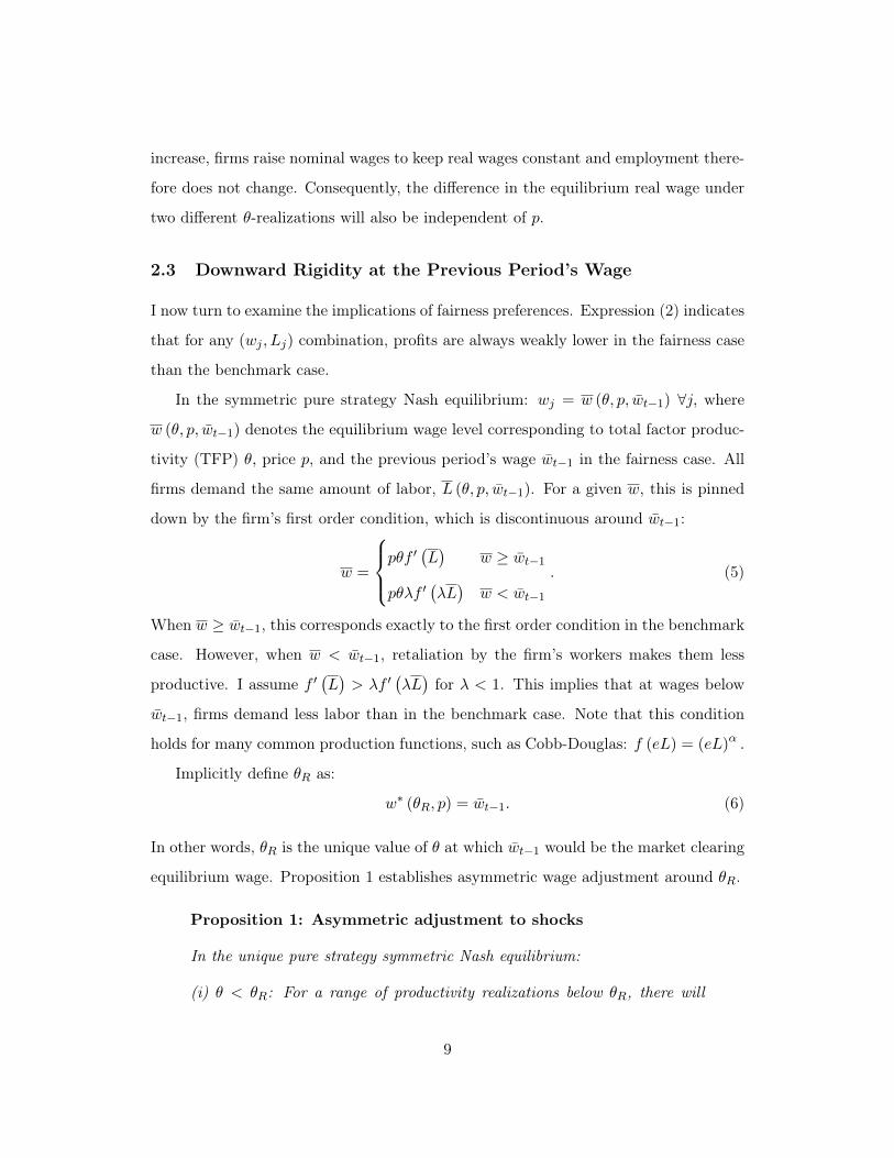
In the symmetric pure strategy Nash equilibrium: wj = w (θ, p, w̄t−1) ∀j, where

w (θ, p, w̄t−1) denotes the equilibrium wage level corresponding to total factor produc-

tivity (TFP) θ, price p, and the previous period’s wage w̄t−1 in the fairness case. All

firms demand the same amount of labor, L (θ, p, w̄t−1). For a given w, this is pinned

down by the firm’s first order condition, which is discontinuous around w̄t−1:

w =

pθf ′

(L)

w ≥ w̄t−1

pθλf ′(λL)

w < w̄t−1

. (5)

When w ≥ w̄t−1, this corresponds exactly to the first order condition in the benchmark

case. However, when w < w̄t−1, retaliation by the firm’s workers makes them less

productive. I assume f ′(L)> λf ′

(λL)for λ < 1. This implies that at wages below

w̄t−1, firms demand less labor than in the benchmark case. Note that this condition

holds for many common production functions, such as Cobb-Douglas: f (eL) = (eL)α .

Implicitly define θR as:

w∗ (θR, p) = w̄t−1. (6)

In other words, θR is the unique value of θ at which w̄t−1 would be the market clearing

equilibrium wage. Proposition 1 establishes asymmetric wage adjustment around θR.

Proposition 1: Asymmetric adjustment to shocks

In the unique pure strategy symmetric Nash equilibrium:

(i) θ < θR: For a range of productivity realizations below θR, there will

9

be no downward wage adjustment. Wages will remain fixed at the previous

period’s wage and there will be excess supply of labor. Specifically, there

exists a θ̃R < θR such that for all θ ∈(θ̃R, θR

), w (θ, p, w̄t−1) = w̄t−1 >

w∗ (θ, p). In addition, limλ→0

θ̃R = 0.

(ii) θ ≥ θR: For any productivity realization above θR, there will be upward

wage adjustment. The equilibrium wage will correspond to the benchmark

case and the labor market will clear: w (θ, p, w̄t−1) = w∗ (θ, p).

Proof: See Appendix B.2. �

For values of θ above θR, firms will increase wages smoothly as θ rises. However, for

sufficiently small decreases in θ below θR, it will be more profitable to maintain wages

at w̄t−1 than to cut wages and have effort decreases due to worker retaliation. However,

if θ falls below θ̃R, w̄t−1 is no longer the unique equilibrium, and wages may fall below

w̄t−1. Note that θ̃R will be lower for smaller values of λ: as λ approaches 0, firms will

never find it profitable to lower wages below w̄t−1.

This contradicts Null hypothesis 1. Proposition 1 predicts that for any two θ′, θ′′ ∈(θ̃R, θR

], the equilibrium wage will be the same: w (θ′, p, w̄t−1) = w (θ′′, p, w̄t−1).

2.4 Impact of Increases in the Previous Period’s Wage

In the benchmark case, previous wages have no impact on period t wages. However,

this will no longer be true when there is reference dependence around the previous

period’s wage. Compare the case of two different lagged wage levels: w̄lowt−1 < w̄hight−1 .

Following equation (6) above, define θhighR implicitly as w∗(θhighR , p

)= w̄hight−1 .

Proposition 2: Ratcheting: Effects of a higher lagged wage

(i) For any θ < θhighR and λ sufficiently small, the period t wage will be

higher and employment will be lower if w̄t−1 = w̄hight−1 than if w̄t−1 = w̄lowt−1.

(ii) For any θ ≥ θhighR , the period t wage and employment levels will be the

same under w̄hight−1 and w̄lowt−1.

Proof: See Appendix B.3. �

10

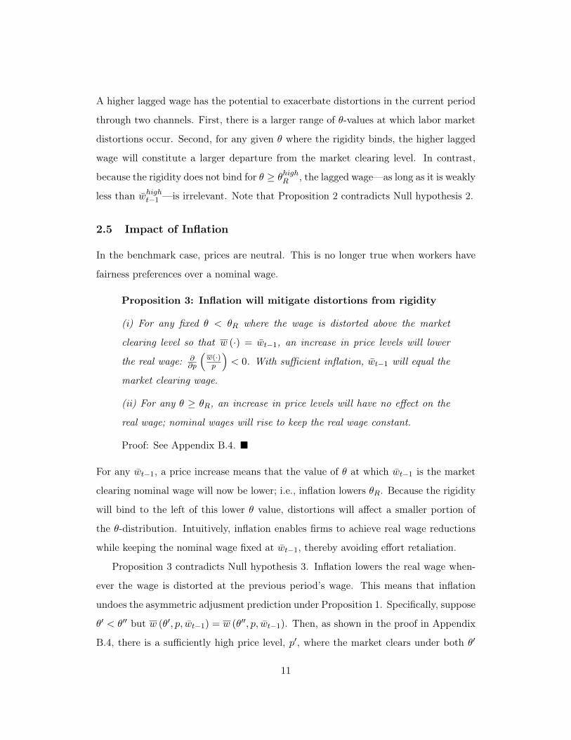
A higher lagged wage has the potential to exacerbate distortions in the current period

through two channels. First, there is a larger range of θ-values at which labor market

distortions occur. Second, for any given θ where the rigidity binds, the higher lagged

wage will constitute a larger departure from the market clearing level. In contrast,

because the rigidity does not bind for θ ≥ θhighR , the lagged wage—as long as it is weakly

less than w̄hight−1 —is irrelevant. Note that Proposition 2 contradicts Null hypothesis 2.

2.5 Impact of Inflation

In the benchmark case, prices are neutral. This is no longer true when workers have

fairness preferences over a nominal wage.

Proposition 3: Inflation will mitigate distortions from rigidity

(i) For any fixed θ < θR where the wage is distorted above the market

clearing level so that w (·) = w̄t−1, an increase in price levels will lower

the real wage: ∂∂p

(w(·)p

)< 0. With sufficient inflation, w̄t−1 will equal the

market clearing wage.

(ii) For any θ ≥ θR, an increase in price levels will have no effect on the

real wage; nominal wages will rise to keep the real wage constant.

Proof: See Appendix B.4. �

For any w̄t−1, a price increase means that the value of θ at which w̄t−1 is the market

clearing nominal wage will now be lower; i.e., inflation lowers θR. Because the rigidity

will bind to the left of this lower θ value, distortions will affect a smaller portion of

the θ-distribution. Intuitively, inflation enables firms to achieve real wage reductions

while keeping the nominal wage fixed at w̄t−1, thereby avoiding effort retaliation.

Proposition 3 contradicts Null hypothesis 3. Inflation lowers the real wage when-

ever the wage is distorted at the previous period’s wage. This means that inflation

undoes the asymmetric adjusment prediction under Proposition 1. Specifically, suppose

θ′ < θ′′ but w (θ′, p, w̄t−1) = w (θ′′, p, w̄t−1). Then, as shown in the proof in Appendix

B.4, there is a sufficiently high price level, p′, where the market clears under both θ′

11

and θ′′. Consequently, after a change in prices to p′, w (θ′, p′, w̄t−1) < w (θ′′, p′′, w̄t−1).

Similarly, inflation will also mitigate the distortion from high lagged wages in Propo-

sition 2. Regardless of the value of θ, with a sufficient increase in prices, w̄t−1 will

be less than the market clearing nominal wage in period t, so that the fairness norm

becomes irrelevant and the rigidity does not bind.

2.6 Discussion

The model assumes that firms make decisions only taking into account current period

payoffs. In a multi-period setting, if there is a high θ-realization, firms would trade off

the benefits of raising wages to satisfy labor demand now, versus the expected decrease

in future profits from the ratcheting effect. In the model, the former consideration

would dominate the latter, producing almost full upward adjustment to positive shocks.

This is because each firm gains the full benefit of posting a higher wage this period, but

only bears a infinitesimal fraction of the cost since its wage contributes negligibly to the

average market wage. In reality, a firm may internalize more of the future costs—e.g.,

if it has long-term relationships with individual workers or if firms can collude to not

raise wages. However, the literature suggests that in the empirical context of this study,

this is unlikely.19 To the extent that this does occur, the core qualitative predictions

that distinguish rigidity from the benchmark case above would still remain, but the

expected magnitude of the effects would be smaller. This would make it less likely

that I would be able to reject the null model in favor of downward nominal rigidity.

In addition, the model assumes the reference point is the previous period’s nominal

wage. Other formulations, such as the expected wage (Koszegi and Rabin 2006), would

alter some of the specific predictions.20 Alternately, consistent with Loewenstein and

Prelec (1991), workers may demand upward sloping wage profiles. This could lead the19For example, Dreze and Mukherjee (1989) observe, “No explicit collusion exists between either

employers or labourers. Individual employers have no monopsonistic power: the pool of employers islarge, and re-sorting of partners occurs constantly.”

20For example, prior positive shocks would not necessarily create ratcheting because the referencepoint would depend on the expected value of θ. Inflation would not affect real wage adjustment if thereference point is formulated with respect to the real wage.

12

reference wage to be of the form w̄t−1 (1 + ϕ), reflecting a norm for a ϕ percentage wage

increase in each period. My formulation of the reference point is simple and matches

the survey evidence provided in Section 6 and in Kahneman et al. (1986). While the

empirical results below do appear to provide support for some types of reference points

as being more likely than others, I take no strong stance on the functional form of the

reference point, or on the micro-foundation for rigidity more generally.

3 Empirical Strategy

3.1 Context: Rural Labor Markets in India

Agricultural production in India, as in most developing countries, is largely undertaken

on smallholder farms. The median household farm size is about 0.9 acres.21 The

composition of farm employment is often a mix of household and hired labor. Markets

for hired labor are active: most households buy and/or sell labor.22 Labor is typically

traded in decentralized markets for casual daily workers. 98% of agricultural wage

employment is through casual wage contracts (with regular/salaried workers making

up the bulk of the remaining 2%). In addition, 67% of landless rural workers report

casual employment as their primary source of earnings.

Within a village, there is typically a gender-specific prevailing wage for casual daily

labor for any given task. This has been documented in earlier development work on

India. For example, Dreze and Mukherjee (1989) state, “[I]n normal times a single wage

rate applies to all adult males in the village for a ’normal’ day’s work, irrespective of the

identity of the partners involved. If the task is of a special nature...some bargaining may

take place.” Similarly, Bliss and Stern (1982) note, “At any particular time everyone

in the village knew what the going rate was. And in nearly every case that wage or

something of equivalent value would be paid to every agricultural laborer.”

Using more recent data, Figure 3 plots the distribution of casual daily wages re-21Unless stated otherwise, the statistics in this sub-section are computed from India’s National

Sample Survey Employment/Unemployment rounds (1982-2009).22See, for example, Rosenzweig (1980), Benjamin (1992), and Bardhan (1997).

13

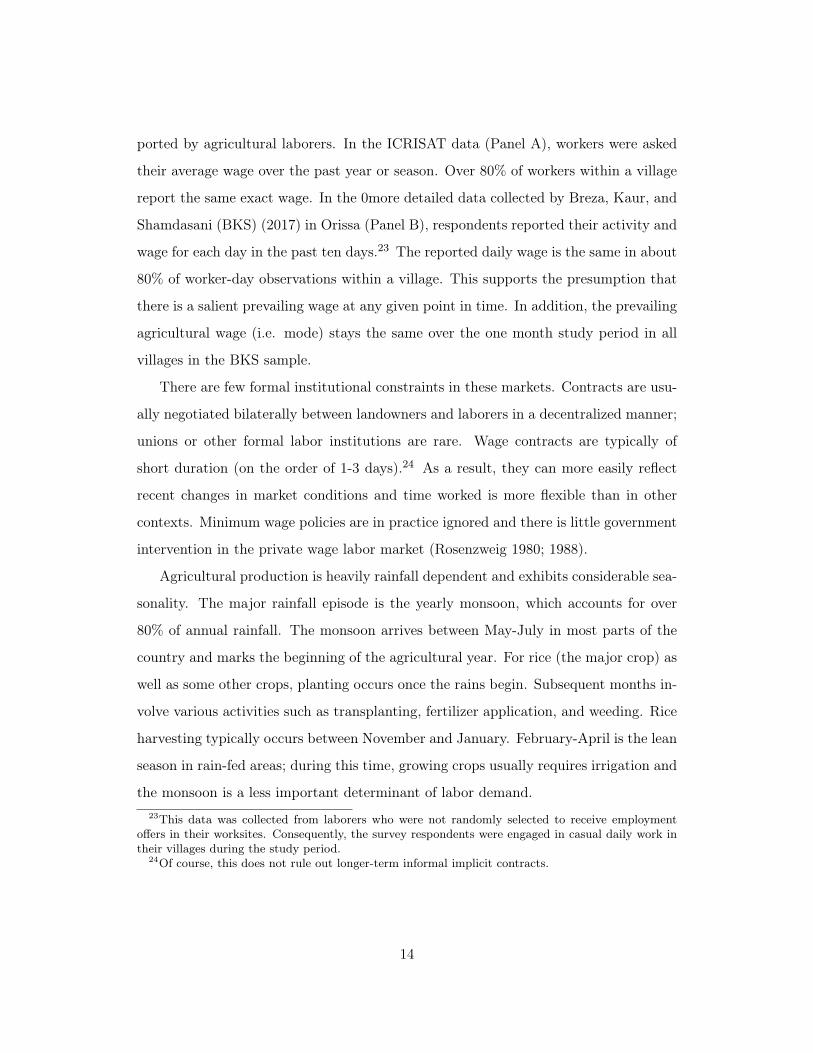
ported by agricultural laborers. In the ICRISAT data (Panel A), workers were asked

their average wage over the past year or season. Over 80% of workers within a village

report the same exact wage. In the 0more detailed data collected by Breza, Kaur, and

Shamdasani (BKS) (2017) in Orissa (Panel B), respondents reported their activity and

wage for each day in the past ten days.23 The reported daily wage is the same in about

80% of worker-day observations within a village. This supports the presumption that

there is a salient prevailing wage at any given point in time. In addition, the prevailing

agricultural wage (i.e. mode) stays the same over the one month study period in all

villages in the BKS sample.

There are few formal institutional constraints in these markets. Contracts are usu-

ally negotiated bilaterally between landowners and laborers in a decentralized manner;

unions or other formal labor institutions are rare. Wage contracts are typically of

short duration (on the order of 1-3 days).24 As a result, they can more easily reflect

recent changes in market conditions and time worked is more flexible than in other

contexts. Minimum wage policies are in practice ignored and there is little government

intervention in the private wage labor market (Rosenzweig 1980; 1988).

Agricultural production is heavily rainfall dependent and exhibits considerable sea-

sonality. The major rainfall episode is the yearly monsoon, which accounts for over

80% of annual rainfall. The monsoon arrives between May-July in most parts of the

country and marks the beginning of the agricultural year. For rice (the major crop) as

well as some other crops, planting occurs once the rains begin. Subsequent months in-

volve various activities such as transplanting, fertilizer application, and weeding. Rice

harvesting typically occurs between November and January. February-April is the lean

season in rain-fed areas; during this time, growing crops usually requires irrigation and

the monsoon is a less important determinant of labor demand.23This data was collected from laborers who were not randomly selected to receive employment

offers in their worksites. Consequently, the survey respondents were engaged in casual daily work intheir villages during the study period.

24Of course, this does not rule out longer-term informal implicit contracts.

14

3.2 Empirical Tests

A distinct labor market is defined as an Indian district (an administrative geographic

unit). Let θdt denote the rainfall realization in district d in year t. The empirical

implementation will focus on discrete shocks. As discussed in Section 3.4, in each year,

a labor market can experience a negative shock (low rainfall), no shock (the usual level

of rainfall), or a positive shock (high rainfall): θdt ∈{θNeg, θZero, θPos

}. I assume

these shocks are i.i.d.: uncorrelated with any other determinants of the wage and

serially uncorrelated across years. In addition, as in the model, I assume the shocks

are transitory: rainfall in a given year affects TFP in only that year.25

In the absence of rigidities, the following simple model captures the effects of tran-

sitory shocks on equilibrium wages:

lnwdt = α0 + α1Posdt + α2Negdt + ln pt + εdt, (7)

where Posdt and Negdt are dummies for a positive and negative shock, respectively.

α1 and α2 give the difference in the wage level under these shocks relative to the

omitted category of Zerodt. Null hypothesis 1 establishes that α1 > 0 and α2 < 0. In

accordance with Null hypothesis 2, lagged values do not appear in equation (7) because

they are irrelevant. Consistent with Null hypothesis 3, prices enter only additively:

a price increase raises the nominal wage to keep the real wage constant. This means

that, for example, the difference in wages between Negdt = 1 and Zerodt = 1 is fixed

at α2; this difference is not affected by inflation. The empirical strategy builds on this

basic specification, which is amenable to the fact that much of the analysis relies on

data from repeated cross-sections over non-consecutive years.26

These null predictions will not hold in the presence of nominal rigidity. Proposition25This is a standard assumption in prior work (e.g., Paxson 1992; Rosenzweig and Wolpin 1993;

Townsend 1994; Jayachandran 2006). Below, I use the results to directly document lack of serialcorrelation in shocks, and to rule out persistent productivity impacts of shocks.

26Note that this equilibrium wage model can also be expressed in a first differences framework.It is straightforward to verify that writing equation (7) for lnwd,t−1 and subtracting from (7) gives:lnwdt− lnwd,t−1 = α1 (Posdt − Posd,t−1)+α2 (Negdt −Negd,t−1)+It+ξdt, where It ≡ ln pt− ln pt−1

is the inflation level. The α1 and α2 coefficients have the same expected value in both specifications.However, equation (7) has the advantage that it does not require data from consecutive years.

15

1 predicts that in equation (7), α2 = 0 if inflation is sufficiently low. Proposition 2

can be tested by adding lagged values. Specifically, the expected value of w̄t−1 will be

higher if there was a positive shock in year t − 1. Proposition 2 (i) therefore implies

that if θd,t−1 = θPos, then in year t, wage distortions can occur for any θdt < θPos (i.e.,

for θNeg and θZero). Model (8) below expands equation (7) by adding dummies for a

lagged positive shock, Posd,t−1, for the cases where θdt = θNeg and θdt = θZero. Thus,

in order to enable separate tests of Propositions 1 and 2, the following specification

breaks up the case of negative shocks into two subcases:

lnwidt = β0 + β1Posdt + β2NonPosd,t−1Negdt + β3Posd,t−1Negdt + β4Posd,t−1Zerodt

+∑K

k=2 φkP̃ osd,t−k + δd + ρt + εidt,

(8)

where where NonPosd,t−1 is an indicator for a non-positive shock last year (i.e.

NonPosd,t−1 ≡ Zerod,t−1 +Negd,t−1), ρt are year fixed effects (which absorb pt), and

δd are district fixed effects that capture differences in real wage levels across districts.

In principle, positive shocks in even earlier years, such as t−2, could distort current

period wages; the power to detect these effects will be lower than from a positive shock

in period t−1 because there is a longer period of time over which inflation can erode the

ratcheting effect (see below). However, such earlier positive shocks could still weaken

the sharpness of the tests of Propositions 1 and 2. To sharpen the predictions, the∑Kk=2 P̃ osd,t−k covariate vector controls for a longer history of lagged positive shocks

from periods t− 2 to t−K. Specifically, P̃ osd,t−k is a binary indicator that equals 1

if there was a positive shock t − k periods ago and no positive shock since then (i.e.

from periods t − k + 1 to period t), and equals 0 otherwise.27 With these controls,

the omitted shock category in model (8) is no shock this year, and non-positive shocks

27Specifically, these controls are defined as: P̃ osd,t−k ≡ Posd,t−k∏tm=t−k+1 (1− Posd,m). Under

rigidities, prior high rainfall shock will only matter if it is not followed by high rainfall in a more recentyear; otherwise the wage would adjust upward later anyway, making the older shock irrelevant. Forthis reason, I use these P̃ osd,t−k controls, rather than just dummies for Posd,t−k. This also increasespower to detect effects on Posdt and Posd,t−1 in the specification. In practice, prior positive shocksoften dissipate within a couple years. Note that it is not necessary to add similar controls for a longerhistory of lagged negative shocks; indeed, the inclusion of such controls makes essentially no differenceto the results.

16

in the past K years. This means that there have been no upward perturbations in

the past wage from high rainfall in earlier years. Consequently, the expected wage

associated with the omitted category approximates the market clearing wage under

no shock: w∗(θZero, p).28 In other words, with this specification, θZero is a proxy for

θR—setting up a direct test of the model’s predictions. This approach allows me to

maximize power for tests by focusing on shocks in periods t− 1 and t, while creating

a “clean” reference value for tests. In the analysis, I show the results with and without

these controls.

Both Null hypothesis 1 and Proposition 1 predict β1 > 0: wages should be higher

when there is a positive shock than under no shock (the omitted category). Thus,

outcomes under high rainfall states will not distinguish rigidities from full adjustment.

β2 provides a test of asymmetric adjustment. Null hypothesis 1 predicts β2 < 0, while

Proposition 1 predicts that β2 = 0 (when inflation is sufficiently low). Note that the

Null hypothesis 1 does not necessarily impose the restriction that β1 = −β2; this will

depend on whether the TFP shock under θNeg and θPos is of equal magnitude, relative

to θZero. To test for asymmetric adjustment, I therefore test Proposition 1 with the

weaker assumption that θNeg < θZero < θPos. If my weaker test fails, then this implies

the more stringent restriction of β1 = −β2 will also fail.

The β3 and β4 coefficients provide tests of Proposition 2. Null hypothesis 2 predicts

that β4 = 0: this year’s TFP is the same as the omitted category and so wages should

be the same. However, under downward rigidities, the wage increase from last year’s

high rainfall would persist into the current year—keeping wages above w∗(θZero, p).

Proposition 2 therefore predicts that β4 > 0: nominal wages will be higher due to the

ratcheting effect. In addition, as was the case for β2, under the null, β3 < 0. However,

Proposition 2 predicts that β3 > 0: wages could be higher than the omitted category

of no shock, even though there is a negative shock in year t.29

28Note that the validity of the empirical strategy does not rely on the wage level under the omittedcategory truly being the market clearing wage. Rather, what is important is that the omitted categorycaptures the counterfactual for the wage under usual rainfall without any ratcheting effects (i.e. noupward distortions) from prior shocks.

29Note that model (8) does not include a separate test for the case of Posd,t−1Posdt. This is because

17

Finally, note that under the null of full adjustment, model (8) should reduce exactly

to model (7): β1 = α1 > 0; β2 = β3 = α2 < 0; and β4 = 0. Thus, equation (8) will

only have additional explanatory power if there are downward rigidities.

Proposition 3 predicts that, in the presence of rigidities, inflation will move wages

closer to market clearing levels. I test this by interacting each of the shock categories

with inflation:

lnwidt = γ0 + γ1Posdt + γ2NonPosd,t−1Negdt + γ3Posd,t−1Negdt + γ4Posd,t−1Zerodt

+ ψ1Posdt × It + ψ2NonPosd,t−1Negdt × It + ψ3Posd,t−1Negdt × It

+ ψ4Posd,t−1Zerodt × It +∑K

k=2 φkP̃ osd,t−k + δd + ρt + εidt,

(9)

where It is price inflation from t − 1 to t. In this model, γ1, γ2, γ3, and γ4 capture

the difference between the omitted category and each respective shock category when

inflation is zero. They therefore provide a sharper test of Propositions 1-2, which

predict γ1 > 0, γ2 = 0, γ3 > 0, and γ4 > 0. The coefficients on the interaction terms

capture how each of these differences changes with inflation.

First, note that because the omitted category approximates w∗(θZero, p), if price

levels rise, the nominal wage in the omitted category will rise accordingly to maintain

a constant real wage. The same will be true when Posdt = 1. Consequently, Null

hypothesis 3 and Proposition 3(ii) both predict that ψ1 = 0: the difference in nominal

wages between Posdt and the omitted category will not change with inflation.

In contrast, inflation will not be neutral in the other shock cases, in which wages

are distorted above market clearing levels. In these cases, employers can keep nomi-

nal wages fixed, enabling real wage reductions through inflation. Consequently, with

inflation, nominal wages will end up being lower under NonPosd,t−1Negdt than the

omitted category: ψ2 < 0. Similarly, inflation will also mitigate the ratcheting effect,

so that lagged transitiory positive shocks do not cause nominal wages to be higher than

under both the null and under rigidities (Proposition 2 (ii)), lagged high rainfall levels will not matterif the rainfall this year is also high. This sub-case is therefore subsumed under Posdt. In general,specification (8) expands model (7) to only include those sub-cases of shocks that can distinguishpredictions under rigidity from the null. This keeps the main estimating equation parismonious.It also helps with statistical power. In the appendix below, I also show results for the full set ofinteractions between lagged and current rainfall levels, which constitute 3× 3 = 9 cells.

18

the omitted category in year t: ψ3 < 0 and ψ4 < 0. In contrast, under Null hypothesis

3, ψ2 = ψ3 = ψ4 = 0. This again means that under the null, specification (9) should

reduce to specification (7).

In addition to providing a direct test of Proposition 3, specification (9) is helpful for

two reasons. Model (8) pools across high and low inflation periods; it will therefore only

have power to distinguish rigidities if average inflation across years is sufficiently low.

Second and relatedly, in model (8), if β2 = 0 but inflation is high (i.e. ρt is positive and

large), then this could mean that nominal wages are rising in absolute terms despite

a negative shock. Under the reference point assumed in Section 2—where workers

dislike wage cuts, but do not demand consistent wage increases-–we would expect this

to happen if inflation is high, but not if it is low. For both these reasons, the level

effects on the shock covariates in model (9) are important because they isolate wage

adjustment in periods of low inflation.

Finally, this empirical strategy allows a test for whether rigidities have real ef-

fects on employment. I replace the dependent variable in model (8) with eidt—the

employment level of worker i in district d in year t:

eidt = σ0 + σ1Posdt + σ2NonPosd,t−1Negdt + σ3Posd,t−1Negdt + σ4Posd,t−1Zerodt

+∑K

k=2 φkP̃ osd,t−k + δd + ρt + εidt.

(10)

Under both the Null hypotheses and Proposition 1, employment should rise with pos-

itive shocks and fall under negative shocks: σ1 > 0 and σ2 < 0.

Testing for employment distortions requires a counterfactual benchmark of what

employment would be if wages could adjust downward. Proposition 2 enables such

a test using lagged transitory positive shocks. Specifically, in the omitted category,

there is no shock in the current year. This therefore serves as a counterfactual for

what employment would be if wages could adjust down after the lagged high rainfall

in the Posd,t−1Zerodt case. If the wage distortion from the ratcheting effect lowers

employment, then σ4 < 0. In contrast, under the null, σ4 = 0. Similarly, Propo-

sition 2 predicts that σ3 < σ2: Posd,t−1Negdt will lead to lower employment than

19

NonPosd,t−1Negdt, because of the additional wage distortion from ratcheting in the

former case. In contrast, under the null, σ3 = σ2.30

It would also be interesting to test whether inflation mitigates employment dis-

tortions. However, because employment data is only available for a small number of

years—providing little variation in inflation—it is not possible to examine differential

employment effects by inflation (see below).

3.3 Data

Wage and employment data is constructed using two primary datasets. The first source

is the rural sample of the Employment/Unemployment rounds of the Indian National

Sample Survey (NSS), a nationally representative survey of over 600 Indian districts.31

Households in each district are sampled on a rolling basis over the agricultural year

(July to June). The survey elicits daily employment and wage information for each

household member over the 7 days preceding the interview. The surveys were con-

ducting during the 1982, 1983, 1987, 1993, 1999, 2003, 2004, 2005, 2007, and 2009

agricultural years.32 The second source is the World Bank Agriculture and Climate

dataset, which provides yearly data on 240 Indian districts in 13 states from 1956-1987.

The unit of observation is a district-year. Rainfall data is taken from Terrestrial Pre-

cipitation: 1900-2008 Gridded Monthly Time Series (version 2.01), constructed by the

Center for Climatic Research, University of Delaware. Appendix C provides further

details on data construction, and Appendix Table 1 provides summary statistics.

3.4 Definition of Shocks

I focus on rainfall in the first month when the monsoon typically arrives in a district

(which ranges from May to July). Focusing on rain in the month of expected arrival30The model also predicts labor rationing under NonPosd,t−1Negdt, but in this case, there is no

clear counterfactual for what employment levels would be if wages were flexible.31A district is an administrative unit in India (like counties in the US). On average, there are 17

districts per state and approximately 2 million residents per district.32Since the monsoon is the rainfall shock used in the analysis, the results will focus on wages and

employment between the month of monsoon arrival and the end of harvesting in January.

20

reflects the fact that both the level of rain and the timeliness of its arrival are important

determinants of productivity. To construct shocks, I compute the rainfall distribution

for each district separately for each dataset: for the years 1956-1987 for the World

Bank data and the years 1982-2009 for the NSS data. A shock is a deviation in rainfall

from a district’s usual rainfall level. Specifically, as in Jayachandran (2006), a positive

shock is rainfall above the eightieth percentile for the district and a negative shock is

rainfall below the twentieth percentile. These discrete cut-offs capture the non-linear

relationship between rainfall and productivity and increase power. This illustrated in

Appendix Figure 1: rainfall in the upper (lower) tail of the distribution is associated

with increased (decreased) yields, while the middle of the rainfall distribution has a

relatively flat relationship with yields.

Rainfall is serially uncorrelated across years (Appendix Table 2). To allow for the

possibility of correlated shocks across districts in a given year, standard errors are

clustered by region-year in all regressions, using the region definitions from the NSS.33

4 Results

4.1 Test for Wage Adjustment

Table 1 provides a preliminary test for wage adjustment (as in model (7)), showing

results from the World Bank and NSS datasets side by side. The dependent variable

is the log nominal daily wage for agricultural work.34 In both datasets, relative to no

shock, nominal wages adjust up when there are positive shocks, but I cannot reject

that they are not lower on average when there is a negative shock (Cols. 1 and 4).35

In Cols. 2 and 5, there is some evidence that a positive shock in one year leads to a

persistent increase in wages in the following year. Under rigidities, a lagged positive33Appendix Table 2 provides some evidence for negative serial correlation in rainfall. Clustering

standard errors by region makes minor difference in the results, and slightly improves precision insome cases. To be conservative, I cluster by region-year.

34The World Bank data provides the average daily cash wage in each district-year. In the NSS data,I compute the daily agricultural wage as total (cash plus in-kind) value of paid earnings for casualagricultural work divided by days worked over the past 7 days. See Appendix C for more details.

35Below, I show that employment does indeed fall sharply when there are negative shocks.

21

shock has the potential to distort wages upward particularly if the current year’s shock

is none or negative. If the current shock is positive, wages would need to adjust up

anyway, rendering the prior positive shock irrelevant. Cols. 3 and 6 limit analysis to

non-positive shocks in the current year—as expected, this increases the magnitude of

the coefficients and lagged positive shocks significantly raise current wages (relative to

having no shock last year) in both datasets. In contrast, consistent with rigidity in the

downward direction, lagged negative shocks have no persistent wage effects.

Table 2 shows the full test corresponding to specification (8). Cols. 1-2 examine

effects in the World Bank data. In Col. 2, relative to the counterfactual of no shock

this year and no shock last year, wages are 4.3% higher if there is positive shock this

year (row 1, significant at the 1% level). In contrast, consistent with Proposition 1,

wages are not significantly lower if there is a negative shock this year: while β2 has a

negative sign, it is small in magnitude and I cannot reject that it is zero (row 2), and

β3 is actually positive (row 3).36 In addition, consistent with Proposition 2, lagged

positive shocks have persistent wage effects (rows 3 and 4). For example, when there

is a positive shock last year and no shock this year, wages are 3.7% higher on average

than if last year’s positive shock had not occurred (significant at the 1% level). The

pattern of findings is similar in the NSS data (Cols. 3-4). Col. 5 limits analysis to

individuals whose primary source of earnings is casual daily labor, with similar results.

Col. 6 adds controls for individual covariates and season of the year. Women earn

substantially less than men, but landholdings and education have no predictive power

for wages.37

I provide a series of robustness checks in the Apendix Tables. The finding of wage

rigidity holds separately for each gender (Appendix Table 5), is robust to limiting anal-

ysis to the cash component of the wage (Appendix Table 6), and appears stronger for36In addition, I reject that β1 = −β2 in both the World Bank data (p-value=0.043) and NSS

data (p-value=0.011). However, as discussed in Section 3.2, this null hypothesis requires strongerassumptions about the production function.

37Appendix Table 3 shows the raw wage change patterns for each shock category using the WorldBank data. The results on wage change premiums are consistent with the findings in Table 2. Ap-pendix Table 4 runs a more detailed version of the main specification in Table 2, with each of the 9shock sequences estimated separately.

22

flat wages relative to piece rate contracts (though the test is under-powered, Appendix

Table 7). In addition, Appendix Tables 8-9 show robustness of these and subsequent

results to alternative percentile cut-offs for defining positive and negative shocks.

4.2 Impact of Inflation on Wage Adjustment

To test Proposition 3, I use the World Bank data since it covers 32 years, providing

substantial variation in inflation. (The NSS rounds are comprised of 8 years of data,

with limited variation in inflation). Inflation is computed from the state-wise Consumer

Price Index for Agricultural Labourers in India, published by the Government of India.

For each district, I construct inflation as the average of inflation in all states excluding

the district’s own state. This captures the component of inflation that is nationally

determined (by factors outside the district’s own state) and therefore unaffected by

local idiosyncratic shocks. Appendix Table 10 verifies that the district rainfall shocks

have no correlation with prices in other states (Cols. 3-4) or inflation in other states

(Col. 5)—the coefficients are small in magnitude and insignificant. The correlation

between own state inflation and national inflation is 0.70.

Table 3, Cols. 1-2 present estimates of model (9), with interactions of each shock

category with the continuous inflation rate in other states. Contemporaneous positive

shocks increase wages (row 1). Consistent with Proposition 3(ii), there are no differen-

tial effects by inflation (row 2). When there are contemporaneous droughts, estimated

wages are the same on average as the omitted category when inflation is zero (row 3).

However, when there is positive inflation, nominal (and real) wages are lower under

negative shocks than when there is no shock (row 4). Similarly, after lagged positive

shocks, wages are ratcheted upwards when inflation is low (rows 5 and 7); as inflation

rises, such shocks are less likely to have persistent effects on current wages (rows 6

and 8). Overall, the negative coefficients on the interaction terms in rows 4, 6, and 8

violate Null hypothesis 3 and are consistent with Proposition 3(i).

In Table 3, Cols. 3-4, the interaction term is a binary indicator for inflation above

6%—about the mean inflation rate in the sample. The pattern of results is similar.

23

Inflation has no differential effects when there are positive shocks, but does enable

downward real wage adjustment in the three categories of shocks where rigidity creates

distortions. As indicated in the F-test p-values at the bottom of the table, when

inflation is above 6%: real wages adjust downward when there are negative shocks

(significant at the 5% level) and I cannot reject that lagged positive shocks have no

effect on current wages.

A potential concern is that there could be co-trends in inflation and the impact of

rainfall shocks. For example, if inflation and the adoption of irrigation (which makes

crops less reliant on rainfall) both trend upward over time, this could create a spurious

correlation. In Appendix Table 11, I conduct two placebo tests to rule out this concern:

interactions of the rainfall shocks with a linear time trend (Col. 2) and with a dummy

for whether the year is after 1970 (the sample mid-point and the beginning of India’s

green revolution, Col. 3) are small and insignificant, indicating that the inflation

results are not driven by co-trends.

4.3 Employment Effects

I test for employment effects on all individuals who comprise the potential agricultural

labor force: rural workers for whom casual employment or self-employment (i.e. work

on their own farm) is a primary or subsidiary activity. 100% of the individuals in the

data who report any positive agricultural work fall within this group. Appendix Table

14 verifies that rainfall does not affect the composition of the sample—e.g., through

the likelihood of reporting oneself as being in the agricultural labor force (Col. 1).

Employment in agriculture is the number of worker-days in the last 7 days (the

interview reference period) in which the individual did any agricultural work: own

farm work plus hired work on someone else’s farm.38 Table 4, Panel A indicates that,

on average, a positive shock in the previous year lowers agricultural employment in38Only 31% of the individuals in the potential agricultural labor force report doing any agricultural

work (on their own land or for someone else) in the past week. Among these individuals, 66% ofworker-days were comprised of work on one’s own land, and the remaining were for work on someoneelse’s land. Note that wages can only be measured for this latter group.

24

the current year. The estimated decrease in agricultural activity is 0.153 days/week or

8.8% for the average worker (Col. 2) and 0.193 days/week or 11% for landless laborers

(Col. 3); these coefficients are significant at the 1% level.

Panel B shows the main specification, equation (10). Contemporaneous positive

shocks (row 1) raise average employment by 0.145 days/week or 8.3%. Contempora-

neous droughts (row 3) decrease employment by 0.094 days/week or 5.4%. Consistent

with the prediction under rigidity, when a drought is preceded by a positive shock

(row 5), employment drops by about 0.254 days/week or 14.6%—more than twice the

magnitude of the decrease in row 3. This difference is statistically significant at the

10% level in Col. 1 and at the 5% level in Col. 2 (see bottom of table). Similarly,

when a year in which there is no shock is preceded by a lagged positive shock (row 7),

this lowers employment by 6-7%.

In village labor markets, those who own land have the right to use their own labor

on their farms before hiring others. As a result, those with little or no land—who are

the net suppliers to the casual daily labor market—are the most likely to be rationed

when rigidities bind. Consistent with this, employment decreases are concentrated

among those with less land (Col. 3). Finally, there is little evidence that the shocks

affect hiring in the non-agricultural sector (Col. 4).

4.4 Separation Failures: Compositional Effects on Employment

A long theoretical literature has pointed out that labor rationing may affect the allo-

cation of labor across firms (Singh, Squire, and Strauss 1986; Benjamin 1992). Specif-

ically, a rationed household’s decision of how much labor to supply and its decision of

how much labor to use in production are no longer separable. Households with smaller

landholdings—which are more likely to face a binding rationing constraint since they

are more reliant on selling labor in the external market—will supply labor more inten-

sively to their own farms. This will lead to a misallocation of labor, with more labor

per acre used in small farms compared to large farms.

In Table 5, I test whether rationing affects the composition of labor supply for

25

agricultural households. I examine effects separately for three groups, defined in terms

of acres per adult in the household:39 the landless, who have no or marginal land (<0.01

acres); below median landholding; and above median landholding. I limit analysis to

observations in which there was a non-positive shock in the current year, since this is

when lagged positive shocks will be most likely to generate rationing.

The dependent variable Col 1. is total worker-days in agriculture—the same mea-

sure as in Table 4. Consistent with the Table 4 results, agricultural employment among

the landless drops substantially. On average, there is no effect on households with be-

low median landholdings; however, this masks substantial changes in labor allocation

for these small landholders. Col. 2 examines effects on hired labor on others’ farms.

In the year after a positive shock, while the landless experience the largest decrease in

wage employment (1.198 days/week), small landholders also experience an estimated

decrease of 0.444 days/week or 22% (significant at the 5% level). Col. 3 indicates

that, at the same time, small landholders increase the amount of time spent working

on their own farms by 0.449 days/week or 18%, significant at the 5% level—this is the

key prediction of the separation failures framework. This magnitude corresponds to

having approximately one extra acre of land (the sample median) in a typical year. In

contrast, large landowners’ labor supply is largely unaffected by lagged positive shocks;

this makes sense since these households do not sell much labor externally.

5 Alternate Explanations

Could the results be explained by reasons other than downward nominal wage rigidity?

First, positive rainfall shocks may have persistent effects on productivity—for ex-

ample by improving future soil moisture. However, then future employment should also

be higher and inflation should not affect persistence, which contradicts the results.39Acres per adult proxies for how much “excess” labor the household would traditionally supply off

its own farm. This is consistent with traditional tests for separation failures, which examine whether,for a given number of acres, households with more adults tend to use more labor on their own farms(e.g., Benjamin 1992, Shapiro 1990, Udry 1996, LaFave and Thomas 2016). Note that I conduct thisanalysis at the household-year level to remain consistent with the previous literature.

26

Second, shocks may affect worker quality. During negative shocks, employers may

hire the subset of workers who are better quality—leading to a higher average wage

per worker. However, this should not depend on inflation. It also cannot explain

why wages do not adjust back down after lagged positive shocks have dissipated. In

addition, I find little evidence that the various shocks change the composition of who

receives wage employment, in terms of gender, education, age, or wealth (Appendix

Table 18).

Third, if positive shocks reduce future labor supply—e.g. through out-migration

or inter-temporal substitution of labor—this could explain why wages rise and em-

ployment falls in the following year. However, to explain the lack of downward wage

adjustment, this would need to (i) occur both in the year after a positive shock and

during a contemporaneous drought and (ii) occur when inflation is low but not when it

is high. It is unclear why labor supply shifters would operate in this way. In addition,

there is no evidence of increased migration after lagged positive shocks or during con-

temporaneous negative shocks in the NSS data (Appendix Table 14) or in the ICRISAT

data (Appendix Table 16).

Fourth, if positive shocks enable credit-constrained small farmers to invest in capi-

tal, this could decrease future labor demand. To fit the results in Table 6, capital would

need to be complementary with own household labor (to explain the increase in own

farm labor supply) and substitutable with hired labor (to explain the large decrease in

hired labor). In this case, wages for hired manual labor should be lower after a lagged

positive shock, not higher. In addition, it is unclear why these effects would occur

only when inflation is low. This explanation also doesn’t account for why downward

wage adjustment is hindered during negative shocks, again only when inflation is low.

Finally, there is little direct evidence that lagged positive shocks lead to an increase in

bullocks, tractors, or fertilizer—among the most common and important capital inputs

in this setting (Appendix Table 19).

Fifth, measurement error (e.g. due to rounding) is unlikely to drive the results. It

is unclear why respondents would be differentially more likely to round wages during

27

negative shocks and the year after positive shocks. In addition, if the wage results

simply reflect reporting errors, we should not observe real employment effects.

Overall, the above arguments are of course suggestive. It is perfectly plausible

that rainfall could affect labor supply or demand through a variety of channels. A

complete investigation of their role is outside the scope of this paper. The model

in this paper delivers a rich set of positive predictions under wage rigidity. The full

pattern of results—for wages, employment, and inflation, along with asymmetry in

effects for each of these tests—is consistent with these predictions.

Finally, efficiency wage models that do not involve nominal rigidities—such as moral

hazard, screening, labor turnover, or nutrition—also generate equilibrium unemploy-

ment. However, they do not predict that wages will be rigid in response to shocks.

For example, none of these models can account for why wages would rise under a pos-

itive shock but then not adjust back down once the shock has dissipated, or why this

should be influenced by inflation. Similar arguments apply to search friction models

that do not incorporate some nominal rigidity. Other models of unemployment—such

as implicit insurance, informal unions, or the fairness efficiency wage model presented

in Section 2—could be consistent with these results if contracting pertains (at least

in part) to the nominal wage. In this paper, I do not take a strong stance on the

micro-foundation for rigidity, but rather argue that a model would need to incorporate

some degree of nominal rigidity to explain the above findings.

6 Mechanisms: Survey Evidence on Fairness Norms

The presence of rigidities in markets for casual daily labor is perhaps especially sur-

prising given the lack of institutional constraints in these markets. This suggests that

non-institutional mechanisms discussed in the literature—such fairness norms against

wage cuts—may play a role in maintaining rigid wages. To obtain suggestive evidence

on the relevance of fairness considerations, I surveyed in 196 agricultural laborers and

200 employers in 34 villages across 6 districts in the Indian states of Orissa and Madhya

28

Pradesh.40 Following Kahneman, Knetsch, and Thaler (1986), I presented scenarios

about wage setting behavior and asked respondents to rate them as “Very fair”, “Fair”,

“Unfair”, or “Very unfair”. Table 6 presents the scenarios and results.41

Panel A establishes baseline norms relating to wage cuts in 2 sets of situations.

For example, question 1 presents a scenario in which a farmer who used to pay Rs.

120/day lowers the wage after a surge in unemployment after a factory (which used to

pay Rs. 100/day) shuts down. The majority of respondents believed it was unfair if

the farmer then re-hires a previous employee at Rs. 100 (62%) or if he hires one of the

newly unemployed factory workers at Rs. 100 (55%).42

Panel B investigates whether norms are anchored on the nominal wage rather than

the real wage. Question 3 presents scenarios that involve a 5% real wage cut due to

a drought, but vary the level of the nominal wage change. 64% of respondents view a

5% nominal wage cut as unfair. However, if there is 5% inflation and no nominal wage

change, 38% view it as unfair. If there is 10% inflation and a 5% nominal wage increase,

the percentage viewing this as unfair drops to 9%.43 Note that similar exercises in the

US and Canada have produced similar patterns, with respondents exhibiting some

(albeit a lesser) degree of “money illusion” (Kahneman et al. 1986; Shafir et al. 1997).

Similarly, 29% of respondents view a real wage cut as unfair if it is achieved by reducing

an in-kind payment of lunch. This is sharply lower than the reactions to a nominal

wage cut of smaller magnitude in Scenario 3A.44

Panel C indicates that several wage setting behaviors associated with market clear-

ing are at odds with expressed fairness norms. For example, 61% of respondents felt40Orissa is one of India’s poorest states, and is dominated by rain-fed paddy. Madhya Pradesh is

more affluent, and a large portion of the survey areas is covered by soybeans, a cash crop.41Each respondent was asked half the questions to prevent the survey from becoming tedious, and

in the case of paired scenarios (1A/1B, 3A/3C, and 9A/9B), was asked only 1 version of the scenario.42In this setting, it is common for some local factories to hire casual daily laborers from surrounding

villages, drawing from the same labor pool as agricultural employers.43In the local vernacular, the term “price of food and clothing” is used to describe inflation. Workers

and employers say that this is frequently cited by workers when they are negotiating wages.44Based on field interviews, the value of the food, when it is provided, usually exceeds Rs. 10. The

responses to Scenario 3A vs. 4 are consistent with evidence that there is lower earnings rigidity (andfewer layoffs during recessions) of workers who receive a base salary plus a bonus, presumably becausebonuses can be more easily cut during downturns (e.g. Kahn 1997).

29

it would be unfair if, during a period of high unemployment, a farmer asks workers for

their reservation wage and then offers a job to the worker with the lowest reservation

wage (Question 5). 63% of respondents think it is unfair for an employer to raise the

wage during a period of high labor demand to attract enough workers, and then lower

the wage to its previous level in later weeks when demand is lower (Question 7).

Finally, Panel D investigates whether respondents think worker effort depends on

fairness perceptions. Question 9 presents a scenario in which a farmer offers a job

to a worker in financial distress. If the job is offered at the prevailing wage (which

would uphold fairness norms and possibly also show benevolence given the laborer’s

distress), 55% percent of respondents say the worker would exert more effort than

usual and only 1% state he would exert less effort than usual. In sharp contrast, if the

wage is below the prevailing rate, only 6% of respondents state the worker would exert

extra effort, while 40% state the worker would exert less effort than usual. Responses

to this question were not substantially different between workers and employers.

Of course, survey responses may not reflect the actual actions people take when the

stakes are real. The pattern of results in Table 6 simply lends some plausibility to the

idea that fairness norms may be a way in which rigid wages are maintained in village

labor markets. It is unclear, however, whether such fairness preferences are inherent

features of utility or whether they arise endogenously—for example, as a coordinating

device among laborers in the presence of incomplete contracting.

Appendix Table 20 tabulates responses to supplementary questions about respon-

dents’ own experiences and behavior. For example, 100% of workers and employers

state that in their memory, there has not been a single year during which the prevailing

nominal agricultural wage for a given season was lower than that in the previous year

(Questions 1 and 6).45 74% of laborers report having been involuntarily unemployed

in the past (Question 2), and 95% of employers claim that they have never hired a45During informal interviews, respondents stated that wages do vary within a year based on the

season/tasks—for example, the transplanting, weeding, harvesting, and lean seasons may each have adistinct wage. They stated that the wage for each season takes as a starting (“reference”) point thewage during that season in the previous year.

30

worker at a wage below the prevailing wage during the lean season (Question 8).

7 Conclusion

This paper tests for downward nominal wage rigidity in markets for casual daily agri-

cultural labor. First, there is asymmetric wage adjustment: nominal wages rise in

response to positive shocks but do not fall during negative shocks. Second, after

transitory positive shocks have dissipated, nominal wages do not return to previous

levels—they remain high in future years. Third, inflation moderates these effects:

when inflation is higher, real wages are more likely to fall during droughts and after

transitory positive shocks. Fourth, wage distortions generate employment distortions,

creating boom and bust cycles: employment is 9% lower in the year after a transitory

positive shock than if the positive shock had not occurred. Fifth, consistent with the

misallocation of labor across farms, households with small landholdings increase labor

supply to their own farms when they are rationed out of the external labor market.

In addition to its broad implications for unemployment and business cycle dynam-

ics, wage rigidity has particular relevance for developing country labor markets. One

focus of the development literature has been that shocks cause shifts in the production

frontier, leading to volatility in income and consumption. In the presence of wage

rigidity, volatility has an additional implication: production may often not be at the

frontier because labor markets do not adjust fully in each period. As implied by the

employment results, this means rigidities may lower the levels and further increase

the volatility of output and income. In addition, the evidence indicates that landless

and marginal farmers—who are the poorest and most vulnerable workers in this set-

ting—bear the brunt of the labor market effects. The findings in Section 4.4 suggest

that this has not only distributional consequences—it can impact labor (mis)allocation,

and consequently is another channel by which rigidities affect aggregate output.

Finding rigidities in casual daily labor markets is perhaps surprising, given the

lack of formal institutional constraints in this setting. The survey evidence suggests

31

that agricultural workers and employers view nominal wage cuts as unfair and believe

that they cause effort reductions. Fairness preferences against wage cuts have been ex-

pressed in a range of contexts, including in richer countries (e.g., Kahneman, Knetsch,

and Thaler 1986). While the strength of the norms expressed in Table 6 appears some-

what higher than that expressed in OECD countries, the survey findings suggest the

potential for some commonality in the reasons for rigidity across settings.

However, it is unclear whether such fairness preferences are inherent features of

utility or whether they arise endogenously. For example, fairness norms may simply

be a coordinating device among workers in a setting where formal contracting or unions

are difficult. Further exploration of the microfoundations for fairness norms is necessary

to fully assess the efficiency and welfare implications of wage rigidity. This in turn,

would inform our understanding of why wage rigidity may appear more prevalent in

some settings than in others.

References

1. Akerlof, George. 2002. “Nobel Lecture: Behavioral Macroeconomics and Macroe-

conomic Behavior.” American Economic Review.

2. Akerlof, George, William Dickens, George Perry. 1996. “The Macroeconomics of

Low Inflation.” Brookings Papers on Economic Activity. 1: 1-76.

3. Akerlof, George, and Janet Yellen. 1990. “The Fair Wage-Effort Hypothesis and

Unemployment,” Quarterly Journal of Economics. 255-83.

4. Altonji, Joseph and Paul Devereux. 2000. “The Extent and Consequences of Down-

ward Nominal Wage Rigidity.” Research in Labor Economics. 19: 383-431.

5. Bardhan, Pranab. 1973. “Size, Productivity, and Returns to Scale: An Analysis of

Farm-level Data in Indian Agriculture.” Journal of Political Economy. 81(6).

6. Barattieri, Alessandro, Susanto Basu, and Peter Gottschalk. 2014. “Some Evidence

on the Importance of Sticky Wages.” AEJ: Macroeconomics.

7. Behrman, Jere. 1999. "Labor Markets in Developing Countries," in ed. O. Ashen-

32

felter and D. Card. (eds), Handbook of Labor Economics, Vol 3: 2859-2939.

8. Benjamin, Dwayne. 1992. “Household Composition, Labor Markets, and Labor

Demand: Testing for Separation in Agricultural Household Models.” Econometrica.

9. Benjamin, Daniel. 2015. “A Theory of Fairness in Labour Markets.” The Japanese

Economic Review. 66(2): 182-225.

10. Bewley, Truman F. 1999. Why Wages Don’t Fall During a Recession.

11. Blanchard, Olivier. 1990. “Why Does Money Affect Output? A Survey”, in Ben

Friedman and Frank Hahn, editors, Handbook of Monetary Economics. Vol 2.

12. Blinder, Alan and Don Choi. 1990. “A Shred of Evidence on Theories of Wage

Stickiness.” Quarterly Journal of Economics, pp. 1003-1015.

13. Bliss, Christopher and Nicholas Stern. 1982. Palanpur: The Economy of an Indian

Village. OUP Catalogue.

14. Breza, Emily, Supreet Kaur, and Yogita Shamdasani. 2017. “The Morale Effects of

Pay Inequality.” NBER Working Paper No. 22491.

15. Bryan, Gharad, Shyamal Chowdhury, and A. Mushfiq Mobarak. 2014. “Under-

Investment in a Profitable Technology: The Case of Seasonal Migration in Bangladesh,”

Econometrica. 82(5): 1671-1748.

16. Card, David. 1990. “Unexpected Inflation, Real Wages, and Employment Determi-

nation in Union Contracts.” American Economic Review.

17. Card, David and Dean Hyslop. 1997. “Does Inflation ‘Grease the Wheels of the

Labor Market’?”, Romer and Romer, Reducing Inflation: Motivation and Strategy.

18. Clarida, Richard, Jordi Galì, and Mark Gertler. 1999. “The Science of Monetary

Policy: A New Keynesian Perspective.” Journal of Economic Literature. 37.

19. Dickens, William et al. 2007. “How Wages Change: Micro Evidence from the

International Wage Flexibility Project.” Journal of Economic Perspectives. 21(2).

20. Dreze, Jean and Anindita Mukherjee. 1989. “Labour Contracts in Rural India:

Theories and Evidence.” The Balance Between Industry and Agriculture in Eco-

nomic Development. Palgrave Macmillan UK. pp. 233-265.

21. Ehrlich, Gabriel and Joshua Montes. 2015. “Wage Rigidity and Employment Out-

33

comes: Evidence from Administrative Data.” Mimeo, University of Michigan.

22. Eliaz, Kfir and Ran Spiegler. 2013. “Reference Dependence and Labor-Market

Fluctuations.” NBER Macroeconomics Annual. Vol. 28.

23. Elsby, Michael. 2009. “Evaluating the Economic Significance of Downward Nominal

Wage Rigidity.” Journal of Monetary Economics. 56.2: 154-169.

24. Elsby, Michael, Donggyun Shin, and Gary Solon. 2016. “Wage Adjustment in the

Great Recession and Other Downturns: Evidence from the United States and Great

Britain.” Journal of Labor Economics. 34.S1: S249-S291.

25. Fallick, Bruce, Michael Lettau, and William Wascher. 2016. “Downward Nominal

Wage Rigidity in the United States During and After the Great Recession.” Mimeo,

Federal Reserve Board.

26. Fehr, Ernst, Lorenz Goette, and Christian Zehnder. 2009. “A Behavioral Account

of the Labor Market: The Role of Fairness Concerns.” Annual Review of Economics.

27. Fink, Gunther, B. Kelsey Jack, and Felix Masiye. 2014. “Seasonal Credit Con-

straints and Agricultural Labor Supply.” NBER Working Paper 20218.

28. Galì, Jordi. 2009. Monetary Policy, Inflation, and the Business Cycle: An Intro-

duction to the New Keynesian Framework. Princeton University Press.

29. Goldberg, Jessica. 2016. “Kwacha Gonna Do? Experimental Evidence about Labor

Supply in Rural Malawi.” American Economic Journal: Applied Economics.

30. Greenwald, Bruce and Joseph Stiglitz. 1987. “Keynesian, New Keynesian and New

Classical Economics.” Oxford Economic Papers. 39(1): 119-133.

31. Hall, Robert and Paul Milgrom. 2008. “The Limited Influence of Unemployment

on the Wage Bargain.” American Economic Review. 98(4): 1653-1674.

32. Holzer, Harry and Edward Montgomery. 1993. "Asymmetries and Rigidities in

Wage Adjustments by Firms." Review of Economics and Statistics. 75(3).

33. Imbert, Clement and John Papp. 2015. “Labor Market Effects of Social Programs:

Evidence from India’s Employment Guarantee.” American Economic Journal: Ap-

plied Economics. 7(2): 233-263.

34. Jayachandran, Seema. 2006. “Selling Labor Low: Wage Responses to Productivity

34

Shocks in Developing Countries.” Journal of Political Economy. 114(3).

35. Kahn, Shulamit. 1997. “Evidence of Nomninal Wage Stickiness from Microdata.”

American Economic Review. 87(5).

36. Kahneman, Daniel, Jack Knetsch, and Richard Thaler. 1986. “Fairness as a Con-

straint on Profit Seeking: Entitlements in the Market.” American Economic Review.

37. Koszegi, Botond and Matthew Rabin. 2006. “A Model of Reference-Dependent

Preferences.” Quarterly Journal of Economics. 121(4): 1133-1166.

38. LaFave, Dan and Duncan Thomas. 2016. “Farms, Families and Markets: New

Evidence on Completeness of Markets in Agricultural Settings.” Econometrica.

84(5):1917-60.

39. Lewis, W. Arthur. 1954. “Economic Development with Unlimited Supplies of

Labour.” The Manchester School. 22(2): 139–191.

40. Leibenstein, Harvey. 1957. Economic Backwardness and Economic Growth.

41. Loewenstein, George and Drazen Prelec. 1991. “Negative Time Preference.” Amer-

ican Economic Review Papers and Proceedings. 81(2): 347-352.

42. Martins, Pedro, Gary Solon, and Jonathan Thomas. 2012. “Measuring What Em-

ployers Do about Entry Wages over the Business Cycle: A New Approach." Amer-

ican Economic Journal: Macroeconomics. 4.4: 36-55.

43. McKenzie, David, Caroline Theoharides, and Dean Yang. 2014. “Distortions in

the International Migrant Labor Market.” American Economic Journal: Applied

Economics. 6(2): 49-75.

44. McLaughlin, Kenneth. 1994. “Rigid Wages?” Journal of Monetary Economics.

45. Mobarak, Mushfiq and Mark Rosenzweig. 2014. “Risk, Insurance and Wages in

General Equilibrium.” NBER Working Paper No. 19811.

46. Morten, Melanie. 2016. “Temporary Migration and Endogenous Risk Sharing in

Village India.” NBER Working Paper No. 22159.

47. Muralidharan, Karthik, Paul Niehaus, and Sandip Sukhtankar. 2016. “General

Equilibrium Effects of (Improving) Public Employment Programs: Experimental

Evidence from India.” Mimeo, UC San Diego.

35

48. Paxson, Christina. 1992. “Using Weather Variability to Estimate the Response of

Savings to Transitory Income in Thailand.” American Economic Review. 82(1).

49. Pissarides, Christopher. 2009. “The Unemployment Volatility Puzzle: Is Wage

Stickiness the Answer?” Econometrica. 77(5): 1339–1369.

50. Pitt Mark and Mark Rosenzweig. 1986. “Agricultural Prices, Food Consumption

and the Health and Productivity of Farmers”, in Agricultural Household Models:

Extensions, Applications, and Policy, pp. 153-182.

51. Rogerson, Richard and Robert Shimer. 2011. “Search in Macroeconomic Models of

the Labor Market”, in Card and Ashenfelter (eds.), Handbook of Labor Economics.

52. Rosenstein-Rodan, P. N. 1956. “Disguised Unemployment and Under-employment

in Agriculture.” Working Papers Series C, Center for International Studies, MIT.

53. Rosenzweig, Mark. 1980. “Neoclassical Theory and the Optimizing Peasant: An

Econometric Analysis of Market Family Labour Supply in Developing Countries.”

Quarterly Journal of Economics. (94): 31–56.

54. Rosenzweig, Mark. 1988. “Labour Markets in Low-income Countries”, in H. Chen-

ery and T. N. Srinivasan (eds), Handbook of Development Economics.

55. Schmitt-Grohé, Stephanie and Martín Uribe. 2013. “Downward Nominal Wage

Rigidity and the Case for Temporary Inflation in the Eurozone.” Journal of Eco-

nomic Perspectives. 27(3): 193–212.

56. Shafir, Eldar, Peter Diamond, and Amos Tversky. 1997. “Money Illusion.” Quar-

terly Journal of Economics. 112(2): 341-374.

57. Shapiro, Charles and Joseph Stiglitz. 1984. “Equilibrium Unemployment as a

Worker Discipline Device.” American Economic Review. 74(3): 433-444.

58. Singh, I., L. Squire and J. Strauss, eds. 1986. Agricultural Household Models:

Extensions, Applications, and Policy. The World Bank, Washington, DC.

59. Tobin, James. 1972. “Inflation and Unemployment.” American Economic Review.

60. Townsend, Robert. 1994. “Risk and Insurance in Village India.” Econometrica.

61. Udry, Chris. 1996. “Efficiency and Market Structure: Testing for Profit Maximiza-

tion in African Agriculture.” Mimeo. Northwestern University.

36

62. Verdugo, Gregory. 2016. “Real Wage Cyclicality in the Eurozone Before and During

the Great Recession: Evidence from Micro Data.” European Economic Review. 82:

46-69.

37

38

Figure 1 – Evolution of the Prevailing Nominal Daily Wage in an Indian Village Notes: 1. This motivational figure plots the prevailing daily nominal wage for ploughing in the Indian village of Tinur, Tamil Nadu during the month of April from 1958-1971. These wages were reported in Agricultural Wages in India, published by the Government of India. 2. The letters “D” and “H” signify years in which there was a drought (rain below the 20th percentile of the district’s historical rainfall distribution) or very good rainfall (rain above the 80th percentile of the district’s historical rainfall distribution), respectively.

Figure 2 – Distributions of Wage Changes

Notes: 1. The figures plot year-to-year percentage changes in agricultural wages in the World Bank Climate and Agriculture dataset. The unit of observation is a district-year, with data on 256 districts from 1956-1987. 2. Nominal wage changes are shown for the full sample (7,680 observations). 3. Real wages are computed as the nominal wage divided by the state CPI for agricultural workers, for the years in which state CPI data is available (6,850 observations). 4. Wage changes are top coded at 50% and bottom coded at –50%.

0.0

5.1

.15

.2.2

5Fr

actio

n of

Obs

erva

tions

-.5 0 .5Percentage Change in Nominal Wage

Nominal Wage Changes

0.0

5.1

.15

.2.2

5Fr

actio

n of

Obs

erva

tions

-.5 0 .5Percentage Change in Real Wage

Real Wage Changes

0.5

1

1.5

2

2.5

3

1958

1959

1960

1961

1962

1963

1964

1965

1966

1967

1968

1969

1970

1971

Nom

inal

Dai

ly W

age

(Rup

ees)

Year

D

H

H

H H

D

D = Drought year H = High (good) rainfall year

39

Figure 3 – Dispersion of Agricultural Wages

Notes: 1. Each panel displays the distribution of: (wage reported by worker) – (gender-specific mode of wages in village). 2. Panel A uses observations from the 2001-2004 ICRISAT Village Level Studies. Respondents were asked to report their average daily wage in the past year or season. Sample is restricted to “Daily wage earners” who report their work type as agricultural labor. Observations are at the worker-year level. N=6 villages, 259 households. 3. Panel B uses data collected by Breza, Kaur, and Shamdasani (2017). Respondents were asked to list their work activity and wage level for each of the past 10 days. Observations are at the worker-day level. N=25 villages, 185 male workers.

Table 1 Effect of Rainfall Shocks on Wages

Dependent Variable: Log Nominal Daily Agricultural Wage Source:

World Bank Data (1956-1987)

Source: National Sample Survey Data (1982-2009)

All observations

All observations

Non-positive shock this year

All observations

All observations

Non-positive shock this year

(1) (2) (3) (4) (5) (6) Positive shock this year 0.021

(0.009)**

0.059 (0.018)***

Negative shock this year -0.004 (0.010)

0.007 (0.023)

Positive shock last year

0.017 (0.009)**

0.026 (0.010)***

0.030 (0.021)

0.050 (0.023)**

Negative shock last year

0.007 (0.009)

-0.001 (0.011)

0.005 (0.022)

0.019 (0.023)

Observations: district-years 7,680 7,680 5,948

-- -- -- Observations: individual-years -- -- -- 59,243 59,243 50,158 Notes: 1. The dependent variable is the log of the nominal daily wage for casual agricultural work. 2. A positive (negative) shock is defined as rainfall in the first month of the monsoon above (below) the 80th (20th) percentile of the district’s usual distribution. No shock is rainfall between the 20th-80th percentile of the district’s usual distribution. 3. Cols (3) and (6) restrict analysis to observations where there was a negative shock or no shock this year. 4. All regressions include district and year fixed effects. Standard errors are clustered by region-year.

0.2

.4.6

.8Fr

actio

n

-40 -20 0 20 40Deviation of own wage from village mode

A. ICRISAT Village Sample

0.2

.4.6

.8Fr

actio

n

-100 -50 0 50 100Deviation of own wage from village mode

B. Orissa Village Sample

40

Table 2 Test for Wage Adjustment

Dependent Variable: Log Nominal Daily Agricultural Wage

Source:

World Bank (1956-1987) Source:

National Sample Survey (1982-2009)

Full sample Full sample

Full sample Full sample Laborers Full sample

(1) (2)

(3) (4) (5) (6)

Last year's shock This year's shock

None, Negative, or Positive Positive 0.026 (0.009)***

0.043 (0.009)***

0.063 (0.018)***

0.072 (0.019)***

0.071 (0.019)***

0.066 (0.016)***

None or Negative Negative -0.011 (0.010)

-0.014 (0.010)

0.001 (0.024)

0.001 (0.023)

0.000 (0.024)

-0.000 (0.022)

Positive Negative 0.035 (0.020)*

0.052 (0.021)**

0.046 (0.042)

0.058 (0.041)

0.064 (0.039)*

0.054 (0.039)

Positive None 0.020 (0.010)**

0.037 (0.011)***

0.058 (0.024)**

0.064 (0.024)***

0.060 (0.025)**

0.064 (0.022)***

Female worker -0.213 (0.028)***

Household land size (acres) 0.0000 (0.0003)

Education 0.0025 (0.0037)

Prior shock history controls? No Yes No Yes Yes Yes Observations: district-years 7,680 7,680 -- -- -- -- Observations: individual-years -- -- 59,243 59,243 51,697 52,278 Dependent variable mean 1.21 1.21 3.39 3.39 3.39 3.39 Notes: 1. The dependent variable is the log of the nominal daily wage for casual agricultural work. 2. A positive (negative) shock is defined as rainfall in the first month of the monsoon above (below) the 80th (20th) percentile of the district’s usual distribution. No shock ("None") is rainfall between the 20th-80th percentile of the district’s usual distribution. 3. The shock sequences are presented as the shock in the previous year and the shock in the current year. Each of the 4 shock covariates are indicators that equal 1 if the sequence of shocks was realized and zero otherwise. The omitted category in each regression is {None or Negative} last year and {None} this year. 4. All regressions include district and year fixed effects. Cols. (2) and (4)-(6) add controls for positive shocks 2 years ago and 3 years ago. Col. (6) includes fixed effects for quarter of the year. Col. (5) limits analysis to individuals whose primary source of earnings is casual daily labor. 5. Standard errors are clustered by region-year.

41

Table 3 Impact of Inflation on Wage Adjustment

Dependent Variable: Log Nominal Daily Agricultural Wage

Inflation measure: Inflation rate

Inflation measure: Indicator: Inflation > 6%

(1) (2)

(3) (4) Last year's shock This year's shock 1 Any Positive 0.027

(0.009)*** 0.043

(0.010)***

0.032 (0.010)***

0.047 (0.011)***

2 Interaction with inflation measure 0.002 (0.095)

0.009 (0.094)

-0.016 (0.019)

-0.013 (0.019)

3 None or Negative Negative 0.005 (0.012)

0.000 (0.012)

0.006 (0.014)

0.001 (0.013)

4 Interaction with inflation measure -0.230 (0.107)**

-0.184 (0.104)*

-0.038 (0.021)*

-0.031 (0.020)

5 Positive Negative 0.067 (0.025)***

0.084 (0.025)***

0.069 (0.028)**

0.085 (0.029)***

6 Interaction with inflation measure -0.481 (0.203)**

-0.479 (0.205)**

-0.083 (0.037)**

-0.082 (0.037)**

7 Positive None 0.041 (0.014)***

0.057 (0.014)***

0.042 (0.015)***

0.057 (0.015)***

8 Interaction with inflation measure -0.257 (0.096)***

-0.248 (0.097)**

-0.047 (0.019)**

-0.045 (0.020)**

Shock history controls No Yes

No Yes Observations: district-years 7680 7680

7680 7680 R2 0.947 0.948

0.947 0.947 F-test p-value: Coefficient 3 + Coefficient 4 = 0 -- --

0.043** 0.049** F-test p-value: Coefficient 5 + Coefficient 6 = 0 -- --

0.566 0.891 F-test p-value: Coefficient 7 + Coefficient 8 = 0 -- --

0.690 0.316 Notes: 1. The dependent variable is the log of the nominal wage for casual daily agricultural work. Observations are from the World Bank data. 2. A positive (negative) shock is defined as rainfall in the first month of the monsoon above (below) the 80th (20th) percentile of the district’s usual distribution. No shock ("None") is rainfall between the 20th-80th percentile of the district’s usual distribution. 3. The shock sequences are presented as the shock in the previous year and the shock in the current year. Each of the 4 shock covariates (rows 1, 3, 5, 7) is an indicator that equals 1 if the sequence of shocks was realized and zero otherwise. The omitted category in each regression is {None or Negative} last year and {None} this year. 4. The remaining covariates (rows 2, 4, 6, 8) are interactions of the shock sequence indicators with a measure of inflation. Inflation is the percentage change in the state CPI for Agricultural Labourers, averaged across all states excluding the district's own state; for 1956 and 1957, the national CPI is used because state CPI data is unavailable. The inflation measure in Cols. (1)-(2) is the continous inflation rate, and in Cols. (3)-(4) is a binary indicator for inflation above 6%. 5. All regressions include district and year fixed effects. Cols. (2) and (4) add controls for positive shocks 2 years ago and 3 years ago. Standard errors are clustered by region-year.

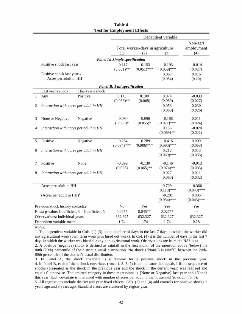
42

Table 4

Test for Employment Effects

Dependent variable

Total worker-days in agriculture

Non-agri employment

(1) (2) (3)

(4) Panel A: Simple specification Positive shock last year -0.117

(0.051)** -0.153

(0.051)*** -0.193

(0.059)***

-0.014 (0.027)

Positive shock last year x Acres per adult in HH

0.067 (0.054)

0.016 (0.20)

Panel B: Full specification

Last year's shock This year's shock 1 Any Positive 0.145

(0.063)** 0.100

(0.068) 0.074

(0.080)

-0.033 (0.027)

2 Interaction with acres per adult in HH 0.053 (0.068)

0.030 (0.026)

3 None or Negative Negative -0.094 (0.055)*

-0.096 (0.055)*

-0.188 (0.071)***

0.011 (0.024)

4 Interaction with acres per adult in HH 0.136 (0.069)**

-0.020 (0.021)

5 Positive Negative -0.254 (0.084)***

-0.289 (0.086)***

-0.416 (0.090)***

0.009 (0.053)

6 Interaction with acres per adult in HH 0.212 (0.060)***

0.013 (0.055)

7 Positive None -0.099 (0.066)

-0.130 (0.065)**

-0.146 (0.074)**

-0.013 (0.035)

8 Interaction with acres per adult in HH 0.027 (0.063)

0.011 (0.032)

Acres per adult in HH 0.709 (0.118)***

-0.386 (0.043)***

(Acres per adult in HH)2 -0.201 (0.034)***

0.085 (0.043)***

Previous shock history controls? No Yes Yes Yes F-test p-value: Coefficient 3 = Coefficient 5 0.087* 0.045** 0.027** -- Observations: individual-years 632,327 632,327 632,327 632,327 Dependent variable mean 1.74 1.74 1.74 0.28 Notes: 1. The dependent variable in Cols. (1)-(3) is the number of days in the last 7 days in which the worker did any agricultural work (own farm work plus hired out work). In Col. (4) it is the number of days in the last 7 days in which the worker was hired for any non-agricultural work. Observations are from the NSS data. 2. A positive (negative) shock is defined as rainfall in the first month of the monsoon above (below) the 80th (20th) percentile of the district’s usual distribution. No shock ("None") is rainfall between the 20th-80th percentile of the district’s usual distribution. 3. In Panel A, the shock covariate is a dummy for a positive shock in the previous year. 4. In Panel B, each of the 4 shock covariates (rows 1, 3, 5, 7) is an indicator that equals 1 if the sequence of shocks (presented as the shock in the previous year and the shock in the current year) was realized and equals 0 otherwise. The omitted category in these regressions is {None or Negative} last year and {None} this year. Each covariate is interacted with number of acres per adult in the household (rows 2, 4, 6, 8). 5. All regressions include district and year fixed effects. Cols. (2) and (4) add controls for positive shocks 2 years ago and 3 years ago. Standard errors are clustered by region-year.

43

Table 5 Compositional Changes in Labor Allocation

Dependent Variable Total worker-days

in agriculture Worker-days as wage laborer

Worker-days on own farm

(1) (2) (3) 1 Positive shock last year -1.729

(0.503)*** -1.198

(0.438)*** -0.531

(0.299)* 2 Positive shock last year x

Below median landholding 1.734

(0.625)*** 0.754

(0.520) 0.980

(0.306)*** 3 Positive shock last year x

Above median landholding 1.289

(0.585)** 1.351

(0.545)** -0.058 (0.410)

Below median landholding -1.017

(0.308)*** -2.107

(0.263)*** 1.092

(0.176)*** Above median landholding -0.618

(0.373)* -4.171

(0.358)*** 3.549

(0.234)***

F-test p-value: Coefficient 1 + Coefficient 2 = 0 0.989 0.046** 0.047** Observations: household-years 166,003 166,003 166,003 Dependent variable mean: Landless & marginal 5.152 5.016 0.136 Dependent variable mean: Below median land 4.179 2.770 1.410 Dependent variable mean: Above median land 5.022 0.882 4.140 Notes: 1. The table decomposes agricultural employment in the past 7 days. The dependent variable in Col. (2) is the number of worker-days household members worked as hired casual wage laborers for others; in Col. (3) it is the number of worker-days household members worked on their own land; and Col. (1) is the total number of worker-days in agriculture (own farm work plus hired out work). Observations are from the NSS data. 2. A positive shock is defined as rainfall in the first month of the monsoon above the 80th percentile of the district’s usual distribution. The sample is comprised of observations in which there is no positive shock this year. 3. The regressions interact the lagged positive shock covariate with binary indicators for landholding categories. The omitted category is landless and marginal landowners--those with less than 0.01 acres per adult in the household. The median landholding is approximately 0.4 acres per adult in the household. 5. All regressions include district and year fixed effects. Standard errors are clustered by region-year.

44

Table 6: Fairness Norms in Rural Labor Markets Proportion of respondents saying the scenario is "unfair" or "very unfair"

All Laborers Employers Panel A: Acceptability of Wage Reductions

1 A farmer hires a laborer to weed his land for 1 day at a wage of Rs. 120. There is a local factory that pays Rs. 100 per day. One month later, the factory shuts down and many people in the area become unemployed.

A) … After this, the farmer decides to do a second weeding and hires the same laborer as before at a wage of Rs. 100.

0.62 0.68 0.57

B) … After this, the farmer decides to do a second weeding and hires one of the newly unemployed laborers at a wage of Rs. 100.

0.55 0.59 0.52

2 A farmer usually pays laborers Rs. 120 per day. His son becomes sick and the medical bills are very expensive. He lowers the wage to Rs. 110 per day.

0.79 0.71 0.87

Panel B: Money Illusion 3 Last year, the prevailing wage in a village was Rs. 100 per day. This year, the rains were very

bad and so crop yields will be lower than usual.

A) … There has been no change in the cost of food and clothing. Farmers decrease this year’s wage rate from Rs. 100 to Rs. 95 per day.

0.64 0.71 0.58

B) …. The price of food and clothing has increased so that what used to cost Rs. 100 before now costs Rs. 105. Farmers keep this year’s wage rate at Rs. 100.

0.38 0.53 0.23

C) … The price of food and clothing has increased since last year, so that what used to cost Rs. 100 before now costs Rs. 110. Farmers increase this year’s wage rate from Rs. 100 to Rs. 105.

0.09 0.09 0.08

4 A farmer usually pays laborers Rs. 100 per day plus food. There is not much work in the area and many laborers are looking for work. He stops providing food but continues to pay Rs. 100.

0.29 0.33 0.24

Panel C: Market Clearing Mechanisms 5 A farmer needs to hire a laborer to plough his land. There is not much work in the area at that

time, and 5 laborers want the job. The farmer asks each of them to state the lowest wage at which they are willing to work, and then hires the laborer who stated the lowest wage.

0.61 0.78 0.44

6 A farmer needs to hire a laborer to plough his land. The prevailing rate in the area is Rs. 120 per day. The farmer knows there is a laborer who needs money to meet a family expense and is having difficulty finding work. The farmer offers the job to that laborer at Rs. 110 per day.

0.53 0.47 0.59

7 It is harvest time and all farmers in a village pay laborers Rs. 120 per day. One large farmer decides to harvest some of his land immediately and needs to hire 10 laborers. To find enough laborers, he pays them Rs. 150 per day for one week. In the following weeks, he decides to harvest the rest of his land, and re-hires 5 of the laborers at Rs. 120 per day.

0.63 0.70 0.57

8 There are 20 landowners in a village. The prevailing wage during ploughing time is Rs. 120. 10 landowners want to attract extra laborers, and they increase the wage they pay to Rs. 130. The other 10 landowners don’t need much labor and maintain the wage at Rs. 120.

0.45 0.52 0.39

Panel D: Fairness Norms and Effort 9 A farmer needs a laborer to weed his land. The prevailing wage is Rs. 120. There isn’t much work in the area and many

want the job. A laborer named Balu has family expenses for which he desperately needs money. The farmer knows Balu’s situation, and offers him the job at: A) Rs. 120 B) Rs. 100. Given his need for money, Balu accepts the job. How carefully will he weed?

More carefully than usual With the normal amount of care Less carefully than usual A) Rs. 120 0.55 0.44 0.01 B) Rs. 100 0.06 0.54 0.40

Notes: 1. The sample is comprised of 196 casual laborers and 200 landowning farmers (employers) from 34 villages across 6 districts in the states of Orissa and Madhya Pradesh. Respondents were working males aged 20-80. 2. Each respondent only received half the scenarios presented in the table. In the case of paired scenarios (questions 1A/1B, 3A/3C, and 9A/9B), each respondent was asked only 1 scenario in each pair. They were asked to rate each scenario as “Very fair”, “Fair”, “Unfair”, or “Very Unfair”. The table reports the proportion selecting “Unfair” or “Very Unfair".

1

ONLINE APPENDICES

APPENDIX A: APPENDIX TABLES AND FIGURES

Appendix Figure 1 – Impact of Rainfall on Log Crop Yield Notes: 1. The figure plots coefficients and 95% confidence intervals from a regression of log crop yields on dummies for each decile of the rainfall distribution. 2. Log crop yields is the log of a weighted average of yields of the 20 crops for which data is available in the World Bank dataset. The yield for each crop has first been normalized by the mean yield of that crop in the district. Weights are the mean percentage of land area planted with a given crop in a district. 3. Each decile dummy equals 1 if rainfall in the first month of the monsoon in the current year fell within the given decile of the district’s usual rainfall distribution for that month and equals 0 otherwise. The confidence interval for the 5th decile, which is the omitted category, is computed by averaging the confidence intervals for the 4th and 6th deciles. 4. Each regression contains district and year fixed effects, and controls for lagged positive and lagged negative shocks in the past 5 years. Analysis is limited to districts with non-positive shocks in the previous year to improve precision. 5. Standard errors are corrected to allow for clustering by region-year.

-0.1

-0.05

0

0.05

0.1

1 2 3 4 5 6 7 8 9 10

Estim

atedIm

pact

(Coefficient)

RainfallDecile

2

Appendix Figure 2 – Relationship between Rainfall and Migration

Notes: 1. Observations are village-years from the ICRISAT VLS 2001-2004 data. 2. The y-axis measures the proportion of households that reported any out migration in a given village-year. 3. The x-axis is standardized deviation of June rainfall (the month of monsoon arrival for all these villages).

Appendix Figure 3 – Proportion of Wages Paid in Cash

Notes: 1. Histogram plots the proportion of the casual agricultural wage payment that was paid in cash. 2. Observations are from the National Sample Survey data.

0.1

.2.3

.4.5

Prop

ortio

n of

hou

seho

lds

with

any

mig

rant

s

-2 -1 0 1 2 3Standardized Rainfall Deviation

0.2

.4.6

Frac

tion

0 .2 .4 .6 .8 1(cash payment) / (cash payment + in-kind payment)

Proportion of Wages Paid in Cash

3

Appendix Table 1 Summary Statistics

Variable Observations

Mean

Standard Deviation

District-years

Individual-years Source

Rainfall shocks % Positive Shock (1956-1987) 0.226 0.418 7,680 -- Univ of Delaware % No Shock (1956-1987) 0.626 0.484 7,680 -- Univ of Delaware % Negative Shock (1956-1987) 0.149 0.356 7,680 -- Univ of Delaware

% Positive Shock (1982-2009) 0.149 0.356 3,548 -- Univ of Delaware % No Shock (1982-2009) 0.627 0.484 3,548 -- Univ of Delaware % Negative Shock (1982-2009) 0.224 0.417 3,548 -- Univ of Delaware Wage and employment variables Log nominal agricultural wage (1956-1987) 1.208 0.817 7,680 -- World Bank Log nominal agricultural wage (1982-2009) 3.390 0.470 -- 59,243 Natl Sample Survey Agricultural employment in past week 1.743 2.783 -- 632,327 Natl Sample Survey Other measures Inflation 0.066 0.095 7,680 -- CPI for Agri Labourers Acres possessed by household 2.750 6.336 -- 632,327 Natl Sample Survey Acres per adult in household 0.633 0.821 -- 632,327 Natl Sample Survey Notes: 1. A positive (negative) shock is defined as rainfall in the first month of the monsoon above (below) the 80th (20th) percentile of the district’s usual distribution. No shock is rainfall between the 20th-80th percentile of the district’s usual distribution. 2. The nominal agricultural wage is the daily wage for casual agricultural work in each dataset. 3. Agricultural employment is the number of worker-days in the past week the individual was employed in agricultural work (either own farm or on someone else's farm). 4. Inflation equals the percentage change in the state-level CPI for Agricultural Labourers from last year to this year. In the years where state CPI is not available, national CPI is used to compute inflation (the years 1956 and 1957).

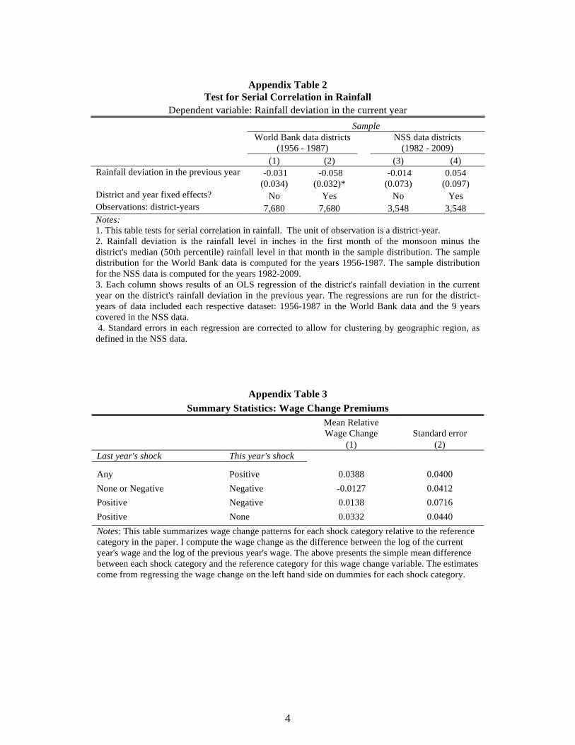
4

Appendix Table 2 Test for Serial Correlation in Rainfall

Dependent variable: Rainfall deviation in the current year

Sample

World Bank data districts (1956 - 1987)

NSS data districts (1982 - 2009)

(1) (2) (3) (4) Rainfall deviation in the previous year -0.031

(0.034) -0.058

(0.032)*

-0.014 (0.073)

0.054 (0.097)

District and year fixed effects? No Yes

No Yes Observations: district-years 7,680 7,680 3,548 3,548 Notes: 1. This table tests for serial correlation in rainfall. The unit of observation is a district-year. 2. Rainfall deviation is the rainfall level in inches in the first month of the monsoon minus the district's median (50th percentile) rainfall level in that month in the sample distribution. The sample distribution for the World Bank data is computed for the years 1956-1987. The sample distribution for the NSS data is computed for the years 1982-2009. 3. Each column shows results of an OLS regression of the district's rainfall deviation in the current year on the district's rainfall deviation in the previous year. The regressions are run for the district-years of data included each respective dataset: 1956-1987 in the World Bank data and the 9 years covered in the NSS data. 4. Standard errors in each regression are corrected to allow for clustering by geographic region, as defined in the NSS data.

Appendix Table 3 Summary Statistics: Wage Change Premiums

Mean Relative Wage Change Standard error

(1) (2)

Last year's shock This year's shock

Any Positive 0.0388 0.0400 None or Negative Negative -0.0127 0.0412 Positive Negative 0.0138 0.0716 Positive None 0.0332 0.0440 Notes: This table summarizes wage change patterns for each shock category relative to the reference category in the paper. I compute the wage change as the difference between the log of the current year's wage and the log of the previous year's wage. The above presents the simple mean difference between each shock category and the reference category for this wage change variable. The estimates come from regressing the wage change on the left hand side on dummies for each shock category.

5

Appendix Table 4 Test for Wage Adjustment: 9-cell Specification

Dependent Variable: Log Nominal Daily Agricultural Wage Source:

World Bank (1956-1987) Source:

NSS (1982-2009) (1) (2) (3)

(4) (5) (6)

Last year's shock This year's shock % Obs % Obs

1 None None 40% Omitted Omitted 39% Omitted Omitted

2 Negative None 8% 0.001 (0.011)

-0.002 (0.011)

12% 0.021 (0.022)

0.020 (0.022)

3 None Positive 14% 0.021

(0.010)** 0.044

(0.011)*** 9% 0.086 (0.019)***

0.086 (0.021)***

4 Negative Positive 3% 0.062 (0.020)***

0.087 (0.020)***

3% 0.093 (0.041)**

0.088 (0.042)**

5 Positive Positive 5% 0.015 (0.016)

0.036 (0.016)**

3% -0.040 (0.034)

-0.041 (0.035)

6 None Negative 8% -0.009 (0.012)

-0.011 (0.012) 11% 0.028

(0.023) 0.024

(0.023)

7 Negative Negative 3% -0.017 (0.017)

-0.019 (0.017)

3% -0.060 (0.051)

-0.059 (0.053)

8 Positive Negative 4% 0.035

(0.020)* 0.059

(0.021)*** 8% 0.058

(0.040) 0.061

(0.039)

9 Positive None 14% 0.020 (0.010)**

0.044 (0.011)***

13% 0.065 (0.023)***

0.064 (0.024)***

Prior shock history controls? -- No Yes -- No Yes Observations: district-years 7,680 7,680 7,680 3,548 -- -- Observations: individual-years -- -- -- -- 59,243 59,243 Notes: 1. The dependent variable is the log of the nominal wage for casual daily agricultural work. 2. A positive (negative) shock is defined as rainfall in the first month of the monsoon above (below) the 80th (20th) percentile of the district’s usual distribution. No shock ("None") is rainfall between the 20th-80th percentile of the district’s usual distribution. 3. The shock sequences are presented as the shock in the previous year and the shock in the current year. Each of the 8 shock covariates is an indicator that equals 1 if the sequence of shocks was realized and equals zero otherwise. The omitted category in each regression is {None} last year and {None} this year. Cols. (1) and (4) indicate the percentage of observations in which each shock sequence was realized. 4. All regressions include district and year fixed effects. Cols. (3) and (6) add controls for positive shocks 2 years ago and 3 years ago. Standard errors are clustered by region-year.

6

Appendix Table 5 Effects by Gender

Dependent Variable: Log Nominal Daily Agricultural Wage

Males Females

(1) (2)

Last year's shock This year's shock Any Positive 0.0860*** 0.0515***

(0.023) (0.017)

None or Negative Negative -0.000143 -0.0132 (0.024) (0.022)

Positive Negative 0.0844* 0.0179 (0.047) (0.036)

Positive None 0.0872*** 0.0426** (0.032) (0.021)

Observations: individual-years 30,201 29,007 R2 0.599 0.570 Notes: 1. This table replicates the main specification separately for male and female laborers. 2. Observations are from the NSS data. Note that the gender variable is missing for 35 observations, which are therefore excluded in this table. 3. All regressions include district and year fixed effects, as well as controls for positive shocks 2 years ago and 3 years ago. 4. Standard errors are clustered by region-year.

7

Appendix Table 6 Effects for Cash vs. In-Kind Wage Payments

Dependent variable:

Dependent variable:

Cash wage payment

In-kind wage payment

Log wage Wage level

Log wage Wage level Proportion

(1) (2)

(3) (4) (5)

Last year's shock This year's shock

Any Positive 0.0718*** 3.144*** -0.0761 -0.586 -0.0185 (0.020) (0.819) (0.078) (0.379) (0.014)

None or Negative Negative -0.0324 -0.609 0.0699 0.612* 0.000516 (0.025) (0.924) (0.077) (0.351) (0.010)

Positive Negative 0.0745 3.853** -0.149 -1.669** -0.0711*** (0.050) (1.812) (0.100) (0.760) (0.026)

Positive None 0.0459** 2.821** -0.109 -0.548 -0.0283** (0.021) (1.422) (0.088) (0.764) (0.013)

Observations: individual-years 48,892 55,825 19,529 55,825 55,825 R2 0.530 0.520 0.618 0.453 0.531 Dependent variable mean 3.297 25.88 2.482 6.167 0.202 Notes: 1. This table replicates the main specification separately for the cash and (monetary value of) the in-kind components of the daily wage payment. 2. The dependent variable in Cols. (1) and (3) is the log of the payment amount. In Cols. (2) and (4) it is the payment level (included for robustness due to the presence of zero cash or in-kind payment levels for some observations). In Col. (5) it is the proportion of the in-kind wage payment: in-kind / total payment. 3. Shocks are defined exactly as in the main specification in the paper. The omitted shock category in each regression is {None or Negative} last year and {None} this year. 4. All regressions include district and year fixed effects, as well as controls for positive shocks 2 years ago and 3 years ago. 5. Standard errors are clustered by region-year. 6. Observations are from NSS data. In round 55 of the survey, information on the cash versus in-kind components of the payment were not separately recorded for some observations; these are omitted from the analysis.

8

Appendix Table 7 Wage Adjustment for Flat Rate vs. Piece Rate Contracts

Dependent Variable: Log Nominal Daily Cash Payment

Rounds with contract type

Rounds with contract type All rounds

(1) (2) (3) Last year's shock This year's shock 1 Any Positive 0.0923** 0.102** 0.120*** (0.041) (0.045) (0.038)

2 Interaction with piece rate dummy -0.0153 -0.0159 -0.00809 (0.072) (0.072) (0.068)

3 None or Negative Negative 0.0306 0.0273 0.0172 (0.040) (0.041) (0.041)

4 Interaction with piece rate dummy -0.0772 -0.0754 -0.0923 (0.092) (0.092) (0.086)

5 Positive Negative 0.0335 0.0690 0.0375 (0.063) (0.062) (0.057)

6 Interaction with piece rate dummy -0.00259 -0.00494 -0.0000641 (0.061) (0.061) (0.057)

7 Positive None 0.111* 0.131** 0.139** (0.065) (0.066) (0.054)

8 Interaction with piece rate dummy -0.117 -0.119 -0.114 (0.106) (0.105) (0.098)

9 Piece rate dummy 0.00634 0.00666 0.00693 (0.030) (0.030) (0.028)

Shock history controls No Yes Yes Observations: district-years 15864 15864 48512

Notes: 1. The dependent variable is the log nominal cash payment for a day of casual agricultural work. 2. Shocks are defined as in the main specifications in the paper. 3. The remaining covariates (rows 2, 4, 6, 8) are interactions of each respective shock sequence indicator with a dummy that equals 1 if the worker was paid a piece rate and equals 0 for a flat wage. 4. In the NSS, contract terms (whether the payment was a flat wage, piece rate, etc.) are only provided in rounds 55, 61, and 66. Cols. (1)-(2) are restricted to observations in which contract terms are defined. To increase power by improving the estimation of the fixed effects, Col. (3) includes observations from all rounds, and adds a full set of interactions of all covariates with a dummy for rounds in which contract terms are not defined; consequently, the displayed coefficients provide the effects for only the rounds of interest (55, 61, 66). 5. All regressions include district and year fixed effects. Cols. (2)-(3) add controls for positive shocks 2 years ago and 3 years ago. Standard errors are clustered by region-year.

9

Appendix Table 8 Robustness to Definition of Rainfall Shocks: NSS Data Results

Percentile Cut-off for Positive/Negative Shocks

80/20 80/25 80/30 75/25 70/30 (1) (2) (3) (4) (5)

Last year's shock This year's shock

Panel A - Dependent Variable: Log Nominal Daily Wage Any Positive 0.072 0.075 0.075 0.067 0.056

(0.019)*** (0.020)*** (0.019)*** (0.019)*** (0.021)***

None or Negative Negative 0.001 0.013 0.013 0.021 0.025 (0.023) (0.021) (0.020) (0.023) (0.024)

Positive Negative 0.058 0.087 0.090 0.063 0.047 (0.041) (0.038)** (0.036)** (0.037)* (0.033)

Positive None 0.064 0.042 0.037 0.054 0.018 (0.024)*** (0.024)* (0.022) (0.022)** (0.023)

Panel B - Dependent Variable: Agricultural Employment Any Positive 0.100 0.093 0.082 0.080 -0.020

(0.068) (0.070) (0.071) (0.066) (0.071)

None or Negative Negative -0.096 -0.089 -0.112 -0.081 -0.111 (0.055)* (0.053)* (0.056)** (0.054) (0.063)*

Positive Negative -0.289 -0.283 -0.308 -0.233 -0.288 (0.086)*** (0.077)*** (0.077)*** (0.073)*** (0.079)***

Positive None -0.130 -0.114 -0.094 -0.047 -0.094 (0.065)** (0.073) (0.075) (0.077) (0.074) Notes: 1. This tables examines robustness of the results to alternate cut-offs for positive and negative shocks in the NSS data. The dependent variable in Panel A is the log of the nominal wage for casual daily agricultural work, and in Panel B is total number of days worked in agriculture (on one's own farm or as a hired laborer on someone else's farm). 2. In each column, positive and negative shocks are defined under different cut-offs, as labeled at the top of each column. E.g., in Col (1), a positive (negative) shock is defined as rainfall in the first month of the monsoon above (below) the 80th (20th) percentile of the district’s usual distribution. This corresponds to the definiton of shocks in the main specification in the paper. Similarly, in Col. (2), a positive (negative) shock is defined as rainfall in the first month of the monsoon above (below) the 80th (25th) percentile of the district’s usual distribution, and so on. 3. All regressions include district and year fixed effects and controls for positive shocks 2 years ago and 3 years ago. 4. Standard errors are clustered by region-year.

10

Appendix Table 9 Robustness to Definition of Rainfall Shocks: World Bank Data Results

Percentile Cut-off for Positive/Negative Shocks

80/20 80/25 80/30 75/25 70/30 (1) (2) (3) (4) (5)

Last year's shock This year's shock Any Positive 0.0474*** 0.0418*** 0.0410*** 0.0445*** 0.0444***

(0.013) (0.010) (0.010) (0.010) (0.011)

Interaction with 1{Inflation> 6%} -0.013 -0.00735 -0.00699 -0.00832 -0.0121 (0.018) (0.018) (0.018) (0.017) (0.016)

None or Negative Negative 0.000586 -0.0123 -0.0139 -0.0137 -0.0188 (0.013) (0.012) (0.012) (0.013) (0.013)

Interaction with 1{Inflation> 6%} -0.0312 -0.0190 -0.0142 -0.0195 -0.0154 (0.020) (0.018) (0.017) (0.018) (0.017)

Positive Negative 0.0849*** 0.0738*** 0.0720*** 0.0743*** 0.0711*** (0.029) (0.026) (0.024) (0.024) (0.021)

Interaction with 1{Inflation> 6%} -0.0816** -0.0714** -0.0572* -0.0678** -0.0594** (0.037) (0.032) (0.030) (0.031) (0.028)

Positive None 0.0573*** 0.0519*** 0.0504*** 0.0510*** 0.0451*** (0.015) (0.016) (0.017) (0.016) (0.015)

Interaction with 1{Inflation> 6%} -0.0445** -0.0397* -0.0432** -0.0422** -0.0489** (0.020) (0.020) (0.021) (0.020) (0.020) F-test p-value: Coeff 3 + Coeff 4 = 0 0.0486 0.0152 0.0184 0.00874 0.00383 F-test p-value: Coeff 5 + Coeff 6 = 0 0.891 0.902 0.434 0.759 0.555 F-test p-value: Coeff 7 + Coeff 8 = 0 0.316 0.356 0.584 0.506 0.780 Notes: 1. This tables examines robustness of the results to alternate cut-offs for positive and negative shocks in the World Bank data. It replicates the regression in Col. (4) of Table 3 under different shock definitions. 2. In each column, positive and negative shocks are defined under different cut-offs, as labeled at the top of each column. E.g., in Col (1), a positive (negative) shock is defined as rainfall in the first month of the monsoon above (below) the 80th (20th) percentile of the district’s usual distribution. This corresponds to the definiton of shocks in the main specification in the paper. Similarly, in Col. (2), a positive (negative) shock is defined as rainfall in the first month of the monsoon above (below) the 80th (25th) percentile of the district’s usual distribution, and so on. 3. All regressions include district and year fixed effects and controls for positive shocks 2 years ago and 3 years ago. 4. Standard errors are clustered by region-year.

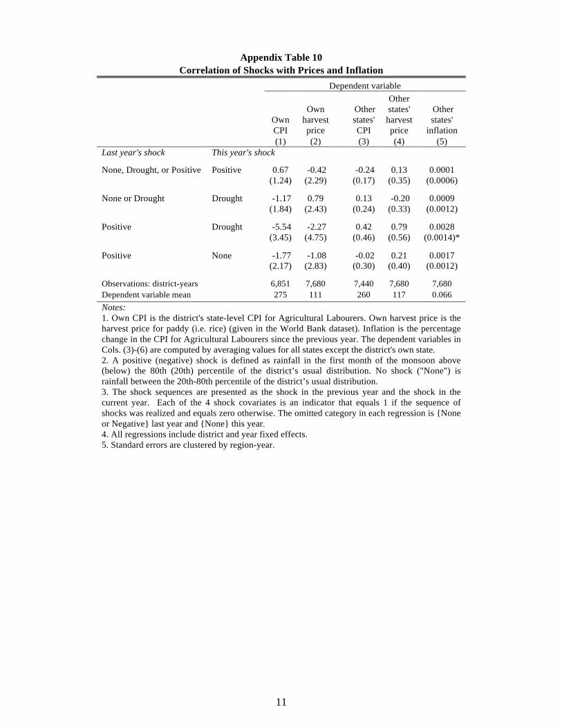
11

Appendix Table 10

Correlation of Shocks with Prices and Inflation

Dependent variable

Own CPI

Own harvest price

Other states' CPI

Other states' harvest price

Other states'

inflation (1) (2) (3) (4) (5) Last year's shock This year's shock

None, Drought, or Positive Positive 0.67 (1.24)

-0.42 (2.29)

-0.24 (0.17)

0.13 (0.35)

0.0001 (0.0006)

None or Drought Drought -1.17 (1.84)

0.79 (2.43)

0.13 (0.24)

-0.20 (0.33)

0.0009 (0.0012)

Positive Drought -5.54 (3.45)

-2.27 (4.75)

0.42 (0.46)

0.79 (0.56)

0.0028 (0.0014)*

Positive None -1.77 (2.17)

-1.08 (2.83)

-0.02 (0.30)

0.21 (0.40)

0.0017 (0.0012)

Observations: district-years 6,851 7,680 7,440 7,680 7,680 Dependent variable mean 275 111 260 117 0.066 Notes: 1. Own CPI is the district's state-level CPI for Agricultural Labourers. Own harvest price is the harvest price for paddy (i.e. rice) (given in the World Bank dataset). Inflation is the percentage change in the CPI for Agricultural Labourers since the previous year. The dependent variables in Cols. (3)-(6) are computed by averaging values for all states except the district's own state. 2. A positive (negative) shock is defined as rainfall in the first month of the monsoon above (below) the 80th (20th) percentile of the district’s usual distribution. No shock ("None") is rainfall between the 20th-80th percentile of the district’s usual distribution. 3. The shock sequences are presented as the shock in the previous year and the shock in the current year. Each of the 4 shock covariates is an indicator that equals 1 if the sequence of shocks was realized and equals zero otherwise. The omitted category in each regression is {None or Negative} last year and {None} this year. 4. All regressions include district and year fixed effects. 5. Standard errors are clustered by region-year.

12

Appendix Table 11 Inflation Results: Robustness and Placebo Checks

Dependent variable: Log nominal daily agricultural wage

Interaction Term in Regressions

Other states' inflation

Linear year trend

Post-1970 dummy

(1) (2) (3) Last year's shock This year's shock 1 None, Drought, or Positive Positive 0.030

(0.009)*** 0.026

(0.009)*** 0.031

(0.013)** 2 Interaction 0.005

(0.012) -0.000 (0.000)

-0.009 (0.017)

3 None or Drought Drought 0.005 (0.012)

-0.012 (0.011)

-0.004 (0.014)

4 Interaction -0.220 (0.109)**

-0.001 (0.001)

-0.016 (0.022)

5 Positive Drought 0.077 (0.025)***

0.035 (0.020)*

0.033 (0.030)

6 Interaction -0.522 (0.199)***

-0.001 (0.003)

0.003 (0.040)

7 Positive None 0.045 (0.014)***

0.020 (0.010)**

0.021 (0.013)

8 Interaction -0.271 (0.096)***

0.000 (0.001)

-0.003 (0.019)

Observations: district-years 7,200 7,680 7,680 R2 0.946 0.947 0.947 Dependent variable mean 1.27 1.21 1.21 Notes: 1. The dependent variable is the log of the nominal wage for casual daily agricultural work. Observations are from the World Bank data. 2. A positive (negative) shock is defined as rainfall in the first month of the monsoon above (below) the 80th (20th) percentile of the district’s usual distribution. No shock ("None") is rainfall between the 20th-80th percentile of the district’s usual distribution. The shock sequences are presented as the shock in the previous year and the shock in the current year. Each of the 4 shock covariates (rows 1, 3, 5, 7) is an indicator that equals 1 if the sequence of shocks was realized and zero otherwise. The omitted category in each regression is {None or Negative} last year and {None} this year. 3. The remaining covariates (rows 2, 4, 6, 8) are interactions with the shock sequence indicators. In Col. (1) the interaction term is inflation, which equals the percentage change in the state CPI for Agricultural Labourers, averaged across all states excluding the district's own state; this is not available for 1956 and 1957. In Col. (2) the interaction term is the calendar year of the observation. In Col. (3), it is a binary indicator for whether the year is after 1970. 4. Regressions include district and year fixed effects. Standard errors are clustered by region-year.

13

Appendix Table 12 Inflation Results: Alternate Inflation Definitions

Dependent variable: Log nominal daily agricultural wage

Interaction Term in Regressions

Current year's inflation

Avg of current and next year's

inflation

Avg of current and previous

year's inflation Current year's

inflation (1) (2) (3) (4)

Last year's shock This year's shock 1 None, Drought, or Positive Positive 0.0474*** 0.0529*** 0.0594*** 0.0440*** (0.011) (0.011) (0.012) (0.010)

2 Interaction -0.0128 -0.0305 -0.0442* -0.0108 (0.019) (0.022) (0.023) (0.019)

3 None or Drought Drought -0.000959 -0.00247 -0.0184 -0.000959 (0.013) (0.015) (0.016) (0.013)

4 Interaction -0.0348 -0.0226 0.00759 -0.0348 (0.023) (0.028) (0.025) (0.023)

5 Positive Drought 0.0847*** 0.0590 0.0987*** 0.0847*** (0.029) (0.039) (0.031) (0.029)

6 Interaction -0.0758** -0.0187 -0.121*** -0.0758** (0.038) (0.062) (0.045) (0.038)

7 Positive None 0.0553*** 0.0534*** 0.0464*** 0.0553*** (0.016) (0.016) (0.015) (0.016)

8 Interaction -0.0334 -0.0457* -0.0219 -0.0334 (0.021) (0.025) (0.022) (0.021)

Sample All All All Exclude 1968 & 1975

Observations: district-years 7,680 7,680 7,680 7,200 Notes: 1. Observations are from the World Bank data. 2. In Cols. (1) and (4), the interaction term is a dummy for inflation>6% in the current calendar year -- Col (1) corresponds to the main specification in the paper. Cols. (2) and (3) average the value of this variable for the current year with the next calendar year (Col. 2) and with the previous calendar year (Col. 3). The robustness checks are similar if the continuous version of variables is used instead. 3. Col (4) drops observations from years 1968 and 1975. 4. Regressions include district and year fixed effects, and controls for positive shocks 2 years ago and 3 years ago. Standard errors are clustered by region-year.

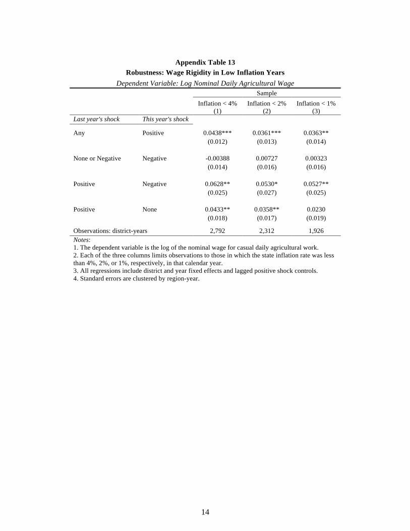
14

Appendix Table 13 Robustness: Wage Rigidity in Low Inflation Years

Dependent Variable: Log Nominal Daily Agricultural Wage

Sample

Inflation < 4% Inflation < 2% Inflation < 1%

(1) (2) (3)

Last year's shock This year's shock Any Positive 0.0438*** 0.0361*** 0.0363**

(0.012) (0.013) (0.014)

None or Negative Negative -0.00388 0.00727 0.00323 (0.014) (0.016) (0.016)

Positive Negative 0.0628** 0.0530* 0.0527** (0.025) (0.027) (0.025)

Positive None 0.0433** 0.0358** 0.0230 (0.018) (0.017) (0.019) Observations: district-years 2,792 2,312 1,926

Notes: 1. The dependent variable is the log of the nominal wage for casual daily agricultural work. 2. Each of the three columns limits observations to those in which the state inflation rate was less than 4%, 2%, or 1%, respectively, in that calendar year. 3. All regressions include district and year fixed effects and lagged positive shock controls. 4. Standard errors are clustered by region-year.

15

Appendix Table 14 Effects of Rainfall on Composition & Size of Agricultural Labor Force

Dependent variable

Individual reports being in agricultural

labor force

Individual migrated into

village

Household member

migrated out of village

(1) (2) (3) Panel A: Simple specification Positive shock last year -0.0034

(0.0039) 0.0018

(0.0021) -0.0037 (0.0026)

Panel B: Full specification

Last year's shock This year's shock Any Positive 0.0027

(0.0047) -0.0047

(0.0017)*** -0.0026 (0.0042)

None or Negative Negative 0.0025 (0.0035)

0.0027 (0.0029)

-0.0053 (0.0132)

Positive Negative -0.0008 (0.0070)

-0.0006 (0.0045)

-0.0061 (0.0128)

Positive None -0.0048 (0.0045)

0.0020 (0.0019)

-0.0047 (0.0031)

Observations: individual-years 1,530,688 414,232 Observations: household-years 36,251 Dependent variable mean 0.389 0.230 0.035 Notes: 1. In Col. (1), the dependent variable is an indicator that equals 1 if the respondent indicated agriculture as his/her primary or subsidiary occupation, and equals 0 otherwise. The sample is comprised of all rural residents from all rounds of the NSS. 2. In Col. (2), the dependent variable is an indicator that equals 1 if the individual is a migrant into the village and 0 otherwise. The sample is comprised of all rural residents in rounds for which questions on individual-level in-migration status were asked (rounds 38, 43, 55). 3. In Col. (3), the dependent variable is an indicator that equals 1 if the household reports having a member who has migrated out in the past year and 0 otherwise. The sample is comprised of all rural households in round 64, which has data on out-migration status by year, surveyed in the final quarter of the agricultural year (so that the 1 year recall links cleanly to agricultural year). 4. A positive (negative) shock is defined as rainfall in the first month of the monsoon above (below) the 80th (20th) percentile of the district’s usual distribution. No shock ("None") is rainfall between the 20th-80th percentile of the district’s usual distribution. 5. In Panel A, the shock covariate is a dummy for a positive shock in the previous year. 6. In Panel B, each of the 4 shock covariates is an indicator that equals 1 if the sequence of shocks (presented as the shock in the previous year and the shock in the current year) was realized and equals zero otherwise. The omitted category in these regressions is {None or Negative} last year and {None} this year. 7. Results are from OLS regressions. Regressions (1) and (2) contain district and year fixed effects. Standard errors are clustered by region-year.

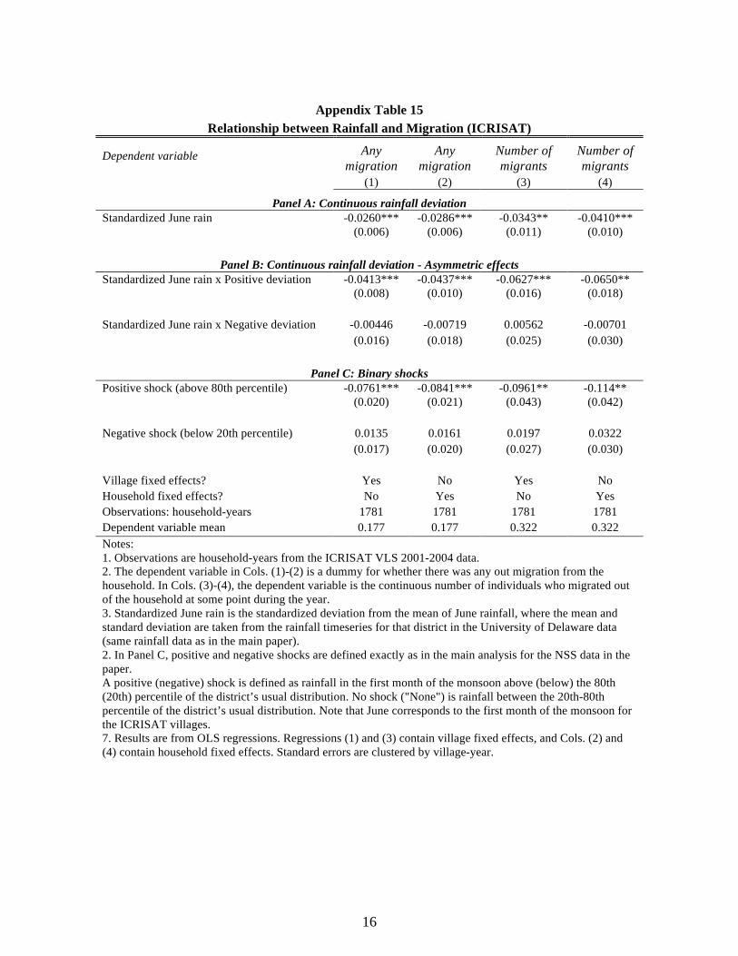
16

Appendix Table 15 Relationship between Rainfall and Migration (ICRISAT)

Dependent variable Any migration

Any migration

Number of migrants

Number of migrants

(1) (2) (3) (4) Panel A: Continuous rainfall deviation

Standardized June rain -0.0260*** -0.0286*** -0.0343** -0.0410*** (0.006) (0.006) (0.011) (0.010)

Panel B: Continuous rainfall deviation - Asymmetric effects Standardized June rain x Positive deviation -0.0413*** -0.0437*** -0.0627*** -0.0650**

(0.008) (0.010) (0.016) (0.018)

Standardized June rain x Negative deviation -0.00446 -0.00719 0.00562 -0.00701 (0.016) (0.018) (0.025) (0.030)

Panel C: Binary shocks Positive shock (above 80th percentile) -0.0761*** -0.0841*** -0.0961** -0.114**

(0.020) (0.021) (0.043) (0.042)

Negative shock (below 20th percentile) 0.0135 0.0161 0.0197 0.0322 (0.017) (0.020) (0.027) (0.030)

Village fixed effects? Yes No Yes No Household fixed effects? No Yes No Yes Observations: household-years 1781 1781 1781 1781 Dependent variable mean 0.177 0.177 0.322 0.322 Notes: 1. Observations are household-years from the ICRISAT VLS 2001-2004 data. 2. The dependent variable in Cols. (1)-(2) is a dummy for whether there was any out migration from the household. In Cols. (3)-(4), the dependent variable is the continuous number of individuals who migrated out of the household at some point during the year. 3. Standardized June rain is the standardized deviation from the mean of June rainfall, where the mean and standard deviation are taken from the rainfall timeseries for that district in the University of Delaware data (same rainfall data as in the main paper). 2. In Panel C, positive and negative shocks are defined exactly as in the main analysis for the NSS data in the paper. A positive (negative) shock is defined as rainfall in the first month of the monsoon above (below) the 80th (20th) percentile of the district’s usual distribution. No shock ("None") is rainfall between the 20th-80th percentile of the district’s usual distribution. Note that June corresponds to the first month of the monsoon for the ICRISAT villages. 7. Results are from OLS regressions. Regressions (1) and (3) contain village fixed effects, and Cols. (2) and (4) contain household fixed effects. Standard errors are clustered by village-year.

17

Appendix Table 16

Effects of Rainfall Shocks on Migration (ICRISAT)

Full sample

Landless & Small farms

Any migration

Any migration

Number of

migrants

Number of

migrants

Any migration

(1) (2) (3) (4) (5) Panel A: Simple specification

Positive shock last year -0.0208 -0.0255 -0.0518 -0.0794 -0.0180 (0.033) (0.040) (0.049) (0.053) (0.029)

Panel B: Full specification Last year's shock This year's shock

Any Positive -0.0654** -0.0731** -0.0976** -0.121** -0.0618** (0.024) (0.025) (0.047) (0.043) (0.026)

None or Negative Negative 0.0212 0.0237 0.0186 0.0273 0.0230 (0.020) (0.023) (0.030) (0.034) (0.026)

Positive Negative -- -- -- -- --

Positive None 0.0354 0.0362 -0.00507 -0.0233 0.0284 (0.032) (0.035) (0.049) (0.058) (0.030)

Village fixed effects? Yes No Yes No Yes Household fixed effects? No Yes No Yes No Observations: household-years 1781 1781 1781 1781 1174 Dependent variable mean 0.177 0.177 0.322 0.322 0.175 Notes: 1. Observations are household-years from the ICRISAT VLS 2001-2004 data. 2. The dependent variable in Cols. (1), (2), and (5) is a dummy for whether there was any out migration from the household. In Cols. (3)-(4), the dependent variable is the continuous number of individuals who migrated out of the household at some point during the year. 3. A positive (negative) shock is defined as rainfall in the first month of the monsoon above (below) the 80th (20th) percentile of the district’s usual distribution. No shock ("None") is rainfall between the 20th-80th percentile of the district’s usual distribution. 4. In Panel A, the shock covariate is a dummy for a positive shock in the previous year. 5. In Panel B, each of the 4 shock covariates is an indicator that equals 1 if the sequence of shocks (presented as the shock in the previous year and the shock in the current year) was realized and equals zero otherwise. 6. Results are from OLS regressions. Cols. (1), (3), and (5) contain village fixed effects, and Cols. (2) and (4) contain household fixed effects. Standard errors are clustered by village-year.

18

Appendix Table 17 Effects of Rain Shocks on Employment over Time Dependent variable: Total worker-days in agriculture

Interaction term (Time measure)

Year (linear) Post 1995 dummy

(1) (2) Panel A: Simple specification Positive shock last year -0.236** -0.143** (0.117) (0.071) Positive shock last year x 0.00591 0.0475 Time measure (0.006) (0.101)

Panel B: Full specification Last year's shock This year's shock

1 Any Positive 0.207 0.105 (0.159) (0.078) 2 Interaction with time measure -0.00318 0.0819 (0.008) (0.133)

3 None or Negative Negative -0.0708 -0.0887 (0.111) (0.067) 4 Interaction with time measure -0.00112 -0.0165 (0.006) (0.117)

5 Positive Negative -0.170 -0.317*** (0.167) (0.103) 6 Interaction with time measure -0.00372 0.0914 (0.009) (0.155)

7 Positive None -0.242* -0.124 (0.143) (0.084) 8 Interaction with time measure 0.00731 0.0492 (0.008) (0.124)

F-test p-value: Coefficient 3 = Coefficient 5 0.087* 0.045** Observations: individual-years 632,327 632,327 Dependent variable mean 1.74 1.74 Notes: 1. Observations are from the NSS data. 2. In Panel A, the shock covariate is a dummy for a positive shock in the previous year. 3. In Panel B, each of the 4 shock covariates (rows 1, 3, 5, 7) is an indicator that equals 1 if the sequence of shocks was realized and equals zero otherwise. 4. In Panel B, rows 2, 4, 6, and 8 show the coefficients from an interaction of each shock with a time measure. In Col (1), the time measure is a continuous linear variable for the year. This variable has been rescaled so that first year in sample (1982) has a value of 1; i.e. the variable is defined as: (year - 1981). In Col (2), the time measure is a dummy for whether the year is after 1995 (the midpoint of the NSS sample). 5. All regressions include district and year fixed effects. Standard errors clustered by region-year.

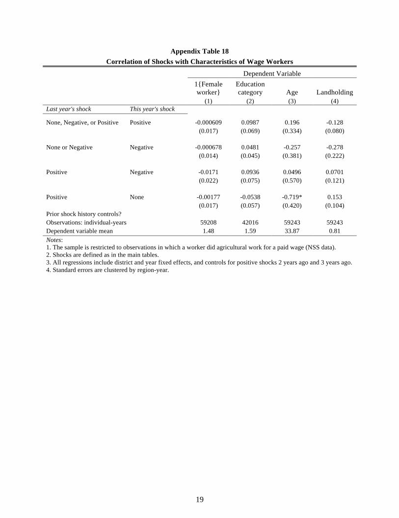
19

Appendix Table 18 Correlation of Shocks with Characteristics of Wage Workers

Dependent Variable

1{Female worker}

Education category Age Landholding

(1) (2) (3) (4)

Last year's shock This year's shock None, Negative, or Positive Positive -0.000609 0.0987 0.196 -0.128

(0.017) (0.069) (0.334) (0.080)

None or Negative Negative -0.000678 0.0481 -0.257 -0.278 (0.014) (0.045) (0.381) (0.222)

Positive Negative -0.0171 0.0936 0.0496 0.0701 (0.022) (0.075) (0.570) (0.121)

Positive None -0.00177 -0.0538 -0.719* 0.153 (0.017) (0.057) (0.420) (0.104)

Prior shock history controls? Observations: individual-years 59208 42016 59243 59243 Dependent variable mean 1.48 1.59 33.87 0.81 Notes: 1. The sample is restricted to observations in which a worker did agricultural work for a paid wage (NSS data). 2. Shocks are defined as in the main tables. 3. All regressions include district and year fixed effects, and controls for positive shocks 2 years ago and 3 years ago. 4. Standard errors are clustered by region-year.

20

Appendix Table 19 Impact of Shocks on Capital Inputs

Dependent variable

Bullocks Tractors Fertilizer

(1) (2) (3)

Panel A: Simple specification Positive shock last year -0.001

(0.010) 0.009

(0.024) -0.004 (0.022)

Panel B: Full specification

Last year's shock This year's shock

None, Drought, or Positive Positive 0.006 (0.011)

-0.012 (0.026)

-0.023 (0.024)

None or Drought Drought -0.012 (0.013)

-0.011 (0.039)

-0.044 (0.036)

Positive Drought -0.012 (0.021)

-0.037 (0.053)

-0.037 (0.045)

Positive None 0.009 (0.011)

0.007 (0.030)

0.005 (0.028)

Observations: district-years 7,680 7,680 7,680 Dependent variable mean 0.000 0.000 0.000 1. The dependent variables are number of bullocks, number of tractors, and amount of nitrogen fertilizer (the most common fertilizer input) used in rural production. The source is the World Bank dataset. All dependent variables are standardized to have a mean of 0 and standard deviation of 1. 2. A positive (negative) shock is defined as rainfall in the first month of the monsoon above (below) the 80th (20th) percentile of the district’s usual distribution. No shock ("None") is rainfall between the 20th-80th percentile of the district’s usual distribution. 3. In Panel A, the shock covariate is a dummy for a positive shock in the previous year. 4. In Panel B, each of the 4 shock covariates (rows 1, 3, 5, 7) is an indicator that equals 1 if the sequence of shocks (presented as the shock in the previous year and the shock in the current year) was realized and equals zero otherwise. The omitted category in these regressions is {None or Negative} last year and {None} this year. Each covariate is interacted with the number of acres per adult in the household (rows 2, 4, 6, 8). 5. All regressions include district and year fixed effects. 6. Standard errors are clustered by region-year.

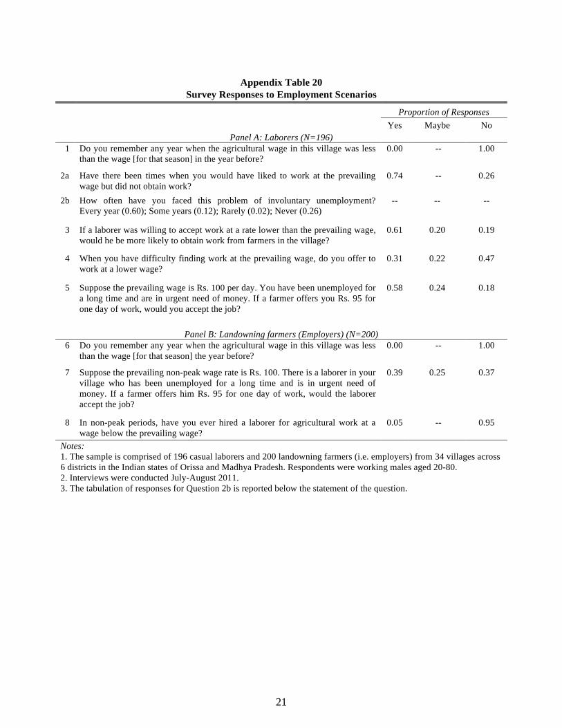
21

Appendix Table 20 Survey Responses to Employment Scenarios

Proportion of Responses Yes Maybe No

Panel A: Laborers (N=196) 1 Do you remember any year when the agricultural wage in this village was less

than the wage [for that season] in the year before? 0.00 -- 1.00

2a Have there been times when you would have liked to work at the prevailing wage but did not obtain work?

0.74 -- 0.26

2b How often have you faced this problem of involuntary unemployment? Every year (0.60); Some years (0.12); Rarely (0.02); Never (0.26)

-- -- --

3 If a laborer was willing to accept work at a rate lower than the prevailing wage, would he be more likely to obtain work from farmers in the village?

0.61 0.20 0.19

4 When you have difficulty finding work at the prevailing wage, do you offer to work at a lower wage?

0.31 0.22 0.47

5 Suppose the prevailing wage is Rs. 100 per day. You have been unemployed for a long time and are in urgent need of money. If a farmer offers you Rs. 95 for one day of work, would you accept the job?

0.58 0.24 0.18

Panel B: Landowning farmers (Employers) (N=200) 6 Do you remember any year when the agricultural wage in this village was less

than the wage [for that season] the year before? 0.00 -- 1.00

7 Suppose the prevailing non-peak wage rate is Rs. 100. There is a laborer in your village who has been unemployed for a long time and is in urgent need of money. If a farmer offers him Rs. 95 for one day of work, would the laborer accept the job?

0.39 0.25 0.37

8 In non-peak periods, have you ever hired a laborer for agricultural work at a wage below the prevailing wage?

0.05 -- 0.95

Notes: 1. The sample is comprised of 196 casual laborers and 200 landowning farmers (i.e. employers) from 34 villages across 6 districts in the Indian states of Orissa and Madhya Pradesh. Respondents were working males aged 20-80. 2. Interviews were conducted July-August 2011. 3. The tabulation of responses for Question 2b is reported below the statement of the question.

For Online Publication

Appendix B: Model Proofs

B.1: Proof of Lemma 1 (Market Clearing in Benchmark Case)

First, I show that the market clearing condition must hold in the benchmark case.

(i) Suppose there is excess labor supply: JL∗ < 1φu(w∗

p

). Then firm j can

cut its wage to some w∗ − ε and still hire L∗ workers. To see this, define δ

as the slack in the market: δ ≡ JL∗ − 1φu(w∗

p

). At wage wj = w∗ − ε, by

the allocation mechanism for workers, the supply of workers available to j

equals the mass of workers that would be willing to work for j minus the

mass of workers employed by the other (higher-wage) firms:

LAvailj = max{

1φu(w∗−εp

)− (J − 1)L∗ , 0

}Firm j can cut wages by ε and still hire L∗ workers as long as ε satisfies

the following condition:

L∗ ≤ 1φu(w∗−εp

)− (J − 1)L∗

=⇒ 1J

[1φu(w∗

p

)− δ]≤ 1

φu(w∗−εp

)− J−1

J

[1φu(w∗

p

)− δ]

=⇒ 1φu(w∗

p

)− δ ≤ 1

φu(w∗−εp

).

Such a wage cut will strictly decrease j’s wage bill while holding revenue

constant, thereby strictly increasing profits. Thus, there cannot be excess

labor supply.

(ii) Suppose there is excess labor demand: JL∗ > 1φu(w∗

p

). This implies

that each firm is hiring strictly less labor than demanded by its first order

condition. If firm j raises its wage infinitesimally above w∗ to w∗+ε, it will

be able to fully satisfy its labor demand by the allocation mechanism. In

what follows, denote LFOCj (wj) as j’s labor demand under wage wj (this is

determined by j’s first order condition, (3)). This upward wage deviation

1

will be profitable if profits from w∗+ ε are higher than profits from w∗, i.e.

if the following inequality holds:

θpf(LFOCj (w∗ + ε)

)−(w∗ + ε)LFOCj (w∗ + ε) > θpf

(1

Jφu

(w∗

p

))−w∗ 1

Jφu

(w∗

p

).

Note that:

limε→0

θpf(LFOCj (w∗ + ε)

)− (w∗ + ε)LFOCj (w∗ + ε)

= θpf(LFOCj (w∗)

)− w∗LFOCj (w∗)

> θpf(

1Jφu(w∗

p

))− w∗ 1

Jφu(w∗

p

).

The equality on the second line follows from the continuity of the first order

condition and continuity of f(•). The inequality on the third line is due to

the fact that at w∗, LFOCj (w∗) maximizes profits. This implies that there

exists some ε̄ > 0 such that for all ε < ε̄, profits from deviating to w∗ + ε

will be higher than maintaining wages at w∗.

Next, I show that no firm will deviate from the w∗ pinned down by conditions (3) and

(4).

(i) Suppose firm j raises its wage to some wj = w∗ + ε. It follows from the

first order condition, (3), that the firm will demand labor LFOCj < L∗.

However, it could have hired LFOCj workers under wage w∗, with a lower

wage bill and higher profits. This deviation cannot be profitable.

(ii) Suppose firm j lowers its wage to some wj = w∗−ε. The supply of workers

available to j equals the mass of workers that would be willing to work for

j minus the mass of workers employed by the other (higher-wage) firms:

LAvailj = max{

1φu(w∗−εp

)− (J − 1)L∗ , 0

}= max

{1φu(w∗−εp

)− J−1

Jφu(w∗

p

), 0}.

Note that at w∗ − ε, LAvailj < L∗ < LFOCj by the above and the first

order condition. This deviation will not be profitable iff πj (w∗, L∗) −

πj

(w∗ − ε, LAvailj

)≥ 0.

2

(a) If LAvailj = 0, then πj

(w∗ − ε, LAvailj

)= 0 and profits are

trivially weakly higher from maintaining w∗.

(b) If LAvailj > 0, then profits from maintaining w∗ will be higher

for J sufficiently large. First, rewrite

πj (w∗, L∗)− πj(w∗ − ε, LAvailj

)= pθ

[f (L∗)− f

(LAvailj

)]− ε

Jφu(w∗

p

)= F (J)− ε

Jφu(w∗

p

),

where I define F (J) as the difference in revenue from L∗ and

LAvailj . Note that:

∂

∂JF (J) =

1

J2φu

(w∗

p

)pθ[f ′(LAvailj

)− f ′ (L∗)

]> 0

by the concavity of f(•). Next, define J̃as:

F (1) =ε

J̃φu

(w∗

p

).

Cutting wages to w∗ − ε will not be a profitable deviation for

any J such that F (J) − εJφu(w∗

p

)> 0. The following shows

this will hold for any J ≥ J̃ . For any positive number X:

F (J̃ +X) > F (J̃) (since ∂∂JF (J) > 0)

> F (1) (since ∂∂JF (J) > 0)

= ε

J̃φu(w∗

p

)(by definition of J̃)

> ε

(J̃+X)φu(w∗

p

).

Thus for J sufficiently large, profits from maintaining w∗ will be higher

than from deviating to w∗ − ε. This is consistent with the assumption

stated in the model that J is arbitrarily large. �

B.2: Proof of Proposition 1 (Asymmetric Adjustment to Shocks)

I prove each of the two parts of Proposition 1 in turn.

(i) Define θ̃R,=w̄t−1

pf ′(

1(J−1)φ

u(λw̄t−1p

)) . For θ ∈(θ̃R, θR

), no firm will deviate

3

from wage offer w̄t−1:

(a) Suppose firm j deviates by raising the wage to wj > w̄t−1. It

follows from the first order condition, (5), that the firm will

demand labor LFOCj < L. However, it could have hired LFOCj

workers under wage w̄t−1, with a lower wage bill and higher

profits. This deviation cannot be profitable.

(b) Suppose firm j deviates by lowering the wage to wj ∈ (λw̄t−1, w̄t−1).

By the firm’s first order condition (5), j′s labor demand will in-

crease, but the supply of labor available to j will decrease to

some LAvailj : 0 < LAvailj < L (θ, p, w̄t−1) . Then:

πj

(wj , L

Availj

)= pθf

(λLAvailj

)− wjLAvailj

< pθf(λLAvailj

)− w̄t−1

(λLAvailj

)(since wj > w̄t−1λ)

< pθf(L (θ, p, w̄t−1)

)− w̄t−1L (θ, p, w̄t−1) (by FOC at w̄t−1)

= πj(w̄t−1, L (θ, p, w̄t−1)

).

This deviation is not profitable.

(c) Suppose firm j deviates by lowering the wage to wj ≤ λw̄t−1.

Since θ > θ′R, the definition of θ′R above implies:

L (θ, p, w̄t−1) >1

(J − 1)φu

(λw̄t−1

p

).

As a result, the supply of labor available to j is:

LAvailj = max{

1φu(wjp

)− (J − 1)L̄ , 0

}≤ max

{1φu(λw̄t−1

p

)− (J − 1)L̄ , 0

}(since wj ≤ w̄t−1λ)

= 0 (by the expression for L above).

The profits from cutting to wj ≤ λw̄t−1 are therefore 0. This

deviation is not profitable.

The first order condition (5) implies that for θ ∈(θ̃R, θR

), L (θ, p, w̄t−1) <

L (θR, p, w̄t−1). This is because the wage remains fixed at w̄t−1, while θ <

θR, and f(·) is concave. Since by the definition of θR, JL (θR, p, w̄t−1) =

4

1φu(w̄t−1

p

), this implies that for θ ∈

(θ̃R, θR

), JL (θ, p, w̄t−1) < 1

φu(w̄t−1

p

).

Thus, there will be excess labor supply in the market.

Finally, note that limλ→0

θ̃R = limλ→0

w̄t−1

pf ′(

1(J−1)φ

u(λw̄t−1p

)) = 0.

(ii) The definition of θR and Lemma 1 imply: w (θR, p, w̄t−1) = w∗ (θR, p) =

w̄t−1. Since ∂w∗(θ,p)∂θ > 0 for all θ, w∗ (θR, p) ≥ w̄t−1 for θ ≥ θR. The

below arguments show that for θ ≥ θR, no firm will want to deviate from

w (θ, p, w̄t−1) = w∗ (θ, p):

(a) Suppose firm j raises its wage to some wj = w (θ, p, w̄t−1)+ε >

w̄t−1. Since wj > w̄t−1, j’s first order condition (5) coincides

with the benchmark case. This deviation cannot be profitable

by the same logic as part (i) of the proof of Proposition 1 above.

(b) Suppose firm j lowers its wage to some wj = w (θ, p, w̄t−1)−ε ≥

w̄t−1. (Note that this implies θ > θR). The firm’s choice of

labor demand at wj is given by first order condition (5). This

deviation cannot be profitable by the same logic as part (ii) of

the proof of Proposition 1 above.

(c) Suppose firm j lowers its wage to some wj = w (θ, p, w̄t−1) −

ε < w̄t−1. Define LFOC,λj implicitly as: pθλf ′(λLFOC,λj

)=

wj . In addition, define LFOC,Bj implicitly as: pθf ′(LFOC,Bj

)=

wj . Note that LFOC,λj < LFOC,Bj because of the assumption

in the model that f ′(L)> λf ′

(λL)for λ < 1. At wj , j’s

optimal labor demand will correspond to LFOC,λj . There are 2

possibilities:

1) If LFOC,λj > LAvailj , then the amount of labor hired by

the firm will correspond to LAvailj (the available labor supply).

Then:

5

πj

(wj , L

Availj

)= pθf

(λLAvailj

)− wjLAvailj

≤ pθf(LAvailj

)− wjLAvailj (since λ < 1)

< pθf (L∗)− w∗L∗ (by Proposition 1 proof)

= pθf(L)− wL

= πj(w,L

)2) If LFOC,λj ≤ LAvailj , then the amount of labor hired by the

firm will correspond to LFOC,λj . Then:

πj

(wj , L

FOC,λj

)= pθf

(λLFOC,λj

)− wjLFOC,λj

< pθf(LFOC,λj

)− wjLFOC,λj (since λ < 1)

< pθf(LFOC,Bj

)− wjLFOC,Bj (by FOC condn (3))

< pθf (L∗)− w∗L∗ (by Proposition 1 proof)

= pθf(L)− wL

= πj(w,L

)Thus, such a downward deviation cannot be profitable.

Since w (θR, p, w̄t−1) = w∗ (θR, p) for θ ≥ θR, this implies L (θR, p, w̄t−1) =

L∗ (θR, p) because labor demand under the first order conditions (3) and (5)

coincides for w ≥ wR. As a result, condition (4) implies JL (θ, p, w̄t−1) =

1φu(w(θ,p,w̄t−1)

p

)for θ ≥ θR. �

B.3: Proof of Proposition 2 (Ratcheting: Distortions from a Higher

Previous Wage)

Following the proof of Proposition 1, define θ̃highR =w̄hight−1

pf ′

(1

(J−1)φu

(λw̄

hight−1p

)) . Following

equation (6), define θlowR implicitly as w∗(θlowR , p

)= w̄lowt−1.

By Proposition 1, w(θ, p, w̄hight−1

)= w̄hight−1 for all θ ∈

(θ̃highR , θhighR

). Since, from

Proposition 1, ∂θ̃highR∂λ > 0 and lim

λ→0θ̃highR = 0, for λ sufficiently small, it follows that

w(θ, p, w̄hight−1

)= w̄hight−1 for θ ≤ θhighR .

6

First note that for θ ∈ (θlowR , θhighR ):

w(θlowR , p, w̄lowt−1

)= w∗

(θlowR , p

)by definition of θaR and Proposition 1

< w∗(θhighR , p

)by Lemma 1

= w̄hight−1 by definition of θbR

.

In addition, for θ ≤ θlowR , w(θ, p, w̄lowt−1

)≤ w̄lowt−1 < w̄hight−1 , where the first inequality

follows from Proposition 1. Together, the above imply that w(θ, p, w̄lowt−1

)< w̄hight−1 for

θ < θhighR .

Since for λ sufficiently small, w(θ, p, w̄hight−1

)= w̄hight−1 for θ < θhighR , this im-

plies: w(θ, p, w̄lowt−1

)< w̄hight−1 = w

(θ, p, w̄hight−1

)for θ < θhighR . Then, L

(θ, p, w̄hight−1

)<

L(θ, p, w̄lowt−1

)for θ < θhighR by the firm’s first order condition (5). �

B.4: Proof of Proposition 3 (Effect of Inflation on Wage Adjustment)

I state the text of Proposition 3(i) formally:

For any fixed θ = θ′ and p = p′ such that w (θ′, p′, w̄t−1) = w̄t−1 >

w∗ (θ′, p′),∂

∂p

(w (θ, p, w̄t−1)

p

) ∣∣∣∣∣θ=θ′,p=p′

< 0.

In addition, ∃ p̃ > p′ such that ∀p ≥ p̃: w (θ′, p, w̄t−1) = w∗ (θ′, p).

The first part of Proposition 3(i) states that when there is a wage distortion, real

wages will fall as price levels rise. First, note that a change in the price level will shift

the θ-interval over which rigidity binds. To make explicit the fact that this interval

depends on p, write this interval as(θ̃(p), θR(p)

). Since the rigidity binds at θ′ and

p′, this implies that θ′ < θR(p′) by Proposition 1. Suppose θ′ ∈(θ̃R(p′), θR(p′)

). For

δ sufficiently small, for any ε ≤ δ, it will be the case that θ′ ∈(θ̃R(p′ + ε), θR(p′ + ε)

)by the fact that θ̃R(p) and θR(p) are continuous in p. Thus, w (θ′, p′ + ε, w̄t−1) = w̄t−1.

As a result, we have:

∂

∂p

(w (θ, p, w̄t−1)

p

) ∣∣∣∣∣θ=θ′,p=p′

= limε→0

w(θ′,p′+ε,w̄t−1)p′+ε − w(θ′,p′,w̄t−1)

p′

ε= lim

ε→0

w̄t−1

p′+ε −w̄t−1

p′

ε< 0.

7

If θ′ ≤ θ̃R(p′), then similar logic applies: an ε increase in the price level, firms will hold

the wage fixed at w̄t−1 (thereby experiencing an increase in profits). Thus, the real

wage will fall with an ε increase in the price level.

The second part of the Proposition 3(i) states that a sufficiently large increase in

the price will enable the market to achieve the market-clearing real wage. To see this,

note that as the price level rises above p′, holding the wage fixed at w̄t−1, labor supply

will fall, while the first order condition (5) implies that labor demand will rise. There

will be a p̃ > p′ at which aggregate labor demand will be exactly equal to aggregate

supply. This p̃ is pinned down by the following condition:

p̃θ′f ′(

1

Jφ̄u

(w̄t−1

p̃

))= w̄t−1.

Note that at p̃ and θ′, w̄t−1 is the market clearing wage. This implies that: w (θ′, p̃, w̄t−1) =

w∗ (θ′, p̃) = w̄t−1. In addition, for any p′′ ≥ p̃:

w (θ′, p̃, w̄t−1) = w̄t−1 by definition of p̃.

= w∗ (θ′, p̃)

≤ w∗ (θ′, p′′) since ∂w∗

∂p > 0

= w (θ′, p′′, w̄t−1) by Proposition 1 since w∗ (θ′, p′′) ≥ w̄t−1

.

Thus, ∀p ≥ p̃, w (θ′, p, w̄t−1) = w∗ (θ′, p) . In addition, this implies L (θ′, p, w̄t−1) =

L∗ (θ′, p) since w (θ′, p, w̄t−1) ≥ w̄t−1 and also implies market clearing by Proposition

1.

The proof of Proposition 3(ii) follows the same logic as in the benchmark case. By

Proposition 1, for any θ > θR, the equilibrium wage corresponds to the market clearing

wage (i.e. w (θ, p, w̄t−1) = w∗ (θ, p) ). It is straightforward to verify from equations (3)

and (4): ∂w∗(θ,p)∂p = w∗

p . Consequently, for any θ > θR, the nominal wage will rise to

keep the real wage constant.�

8

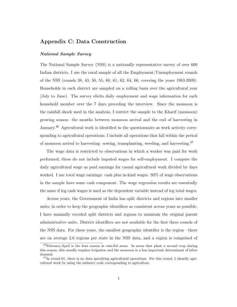
Appendix C: Data Construction

National Sample Survey

The National Sample Survey (NSS) is a nationally representative survey of over 600

Indian districts. I use the rural sample of all the Employment/Unemployment rounds

of the NSS (rounds 38, 43, 50, 55, 60, 61, 62, 64, 66, covering the years 1983-2009).

Households in each district are sampled on a rolling basis over the agricultural year

(July to June). The survey elicits daily employment and wage information for each

household member over the 7 days preceding the interview. Since the monsoon is

the rainfall shock used in the analysis, I restrict the sample to the Kharif (monsoon)

growing season: the months between monsoon arrival and the end of harvesting in

January.46 Agricultural work is identified in the questionnaire as work activity corre-

sponding to agricultural operations; I include all operations that fall within the period

of monsoon arrival to harvesting: sowing, transplanting, weeding, and harvesting.47

The wage data is restricted to observations in which a worker was paid for work

performed; these do not include imputed wages for self-employment. I compute the

daily agricultural wage as paid earnings for casual agricultural work divided by days

worked. I use total wage earnings: cash plus in-kind wages. 93% of wage observations

in the sample have some cash component. The wage regression results are essentially

the same if log cash wages is used as the dependent variable instead of log total wages.

Across years, the Government of India has split districts and regions into smaller

units; in order to keep the geographic identifiers as consistent across years as possible,

I have manually recoded split districts and regions to maintain the original parent

administrative units. District identifiers are not available for the first three rounds of

the NSS data. For these years, the smallest geographic identifier is the region—there

are on average 2.6 regions per state in the NSS data, and a region is comprised of46February-April is the lean season in rain-fed areas. In areas that plant a second crop during

this season, this usually requires irrigation and the monsoon is a less important determinant of labordemand.

47In round 61, there is no data specifying agricultural operations. For this round, I identify agri-cultural work by using the industry code corresponding to agriculture.

1

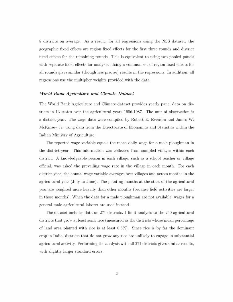
8 districts on average. As a result, for all regressions using the NSS dataset, the

geographic fixed effects are region fixed effects for the first three rounds and district

fixed effects for the remaining rounds. This is equivalent to using two pooled panels

with separate fixed effects for analysis. Using a common set of region fixed effects for

all rounds gives similar (though less precise) results in the regressions. In addition, all

regressions use the multiplier weights provided with the data.

World Bank Agriculture and Climate Dataset

The World Bank Agriculture and Climate dataset provides yearly panel data on dis-

tricts in 13 states over the agricultural years 1956-1987. The unit of observation is

a district-year. The wage data were compiled by Robert E. Evenson and James W.

McKinsey Jr. using data from the Directorate of Economics and Statistics within the

Indian Ministry of Agriculture.

The reported wage variable equals the mean daily wage for a male ploughman in

the district-year. This information was collected from sampled villages within each

district. A knowledgeable person in each village, such as a school teacher or village

official, was asked the prevailing wage rate in the village in each month. For each

district-year, the annual wage variable averages over villages and across months in the

agricultural year (July to June). The planting months at the start of the agricultural

year are weighted more heavily than other months (because field activities are larger

in those months). When the data for a male ploughman are not available, wages for a

general male agricultural laborer are used instead.

The dataset includes data on 271 districts. I limit analysis to the 240 agricultural

districts that grow at least some rice (measured as the districts whose mean percentage

of land area planted with rice is at least 0.5%). Since rice is by far the dominant

crop in India, districts that do not grow any rice are unlikely to engage in substantial

agricultural activity. Performing the analysis with all 271 districts gives similar results,

with slightly larger standard errors.

2

Rainfall Data

Rainfall data is taken from Terrestrial Precipitation: 1900-2008 Gridded Monthly Time

Series (version 2.01), constructed by Cort J. Willmott and Kenji Matsuura at the Cen-

ter for Climatic Research, University of Delaware. Rainfall estimates are constructed

for 0.5 by 0.5 degree latitude-longitude grids by interpolating from 20 nearby weather

stations. I match the geographic center of each district to the nearest latitude-longitude

node in the rain data. These district coordinates are included in the World Bank data;

for the NSS data, I have obtained them using district boundaries from the Census of

India.

Consumer Price Index Data

Inflation is computed from the state-wise Consumer Price Index for Agricultural Labour-

ers in India, published by the Government of India. Inflation in year t is the percentage

change in the state CPI from calendar year t-1 to calendar year t. State-level CPI data

is not available before the year 1957. Thus, for the years 1956 and 1957, I use national

CPI numbers and use the national inflation rate across the whole country in the regres-

sions. Omitting these 2 years in the analysis has little effect on the findings (Appendix

Table 6, Col. 1).

3