The Timing of Pay

Christopher A. Parsons and Edward D. Van Wesep1

October 2011

1Christopher Parsons, Rady School of Management, University of California at San Diego. email: ca-parsons@ucsd.edu. phone: 919-265-9246. Edward Van Wesep, University of North Carolina at Chapel Hill�sKenan-Flagler Business School. email: vanwesep@unc.edu. phone: 919-360-9689.

Abstract

There exists large and persistent variation in not only how, but when employees are paid, a fact

unexplained by existing theory. This paper develops a simple model of optimal pay timing for �rms.

When workers have self-control problems, they under-save and experience volatile consumption

between paychecks. Thus, pay whose delivery matches the timing of workers�consumption needs

will reduce wage costs. The model also explains why pay timing should be regulated (as it is in

practice): although the worker bene�ts from a timing pro�le that smoothes her consumption, her

lack of self-control induces her to attempt to undo the arrangement, either by renegotiating with

her employer or taking out payday loans. Regulation of pay timing and consumer borrowing is

required to counter these e¤orts, helping the worker help herself.

Keywords: Compensation, Hyperbolic Discounting, Welfare, Payday Lending

JEL: H53, I38, J31, J33

Pay him his wages each day before sunset, because he is poor and is counting on it. Otherwise he may

cry to the Lord against you, and you will be guilty of sin.

�Deuteronomy 24:15

Wages can vary along three dimensions. Level di¤erences, such as a car salesman earning $40,000

versus a librarian earning $30,000, are usually attributed to workers having di¤erent value marginal

products or outside options.1 Structure di¤erences, such as a bartender being paid mostly in tips

versus a salaried postal worker, typically arise in response to incentive or information problems.

Timing di¤erences, the subject of this paper, are variations in the temporal patterns of when pay,

for a given level and structure, is disbursed to employees. Examples would include a farm issuing

laborers weekly, instead of monthly, paychecks, a bank awarding bonuses to its tellers around

Christmas, or a university spreading out a professor�s nine month salary over twelve months.

In contrast to an extensive theoretical literature on the �rst two dimensions, there is a compar-

ative absence with respect to pay timing. This paper is an initial attempt to address this void.

Our analysis is motivated by two facts. First, under standard assumptions, the timing of wage

payments should not matter� workers can save or borrow to create any timing pro�le they desire�

but the data suggest otherwise. The timing of bonuses is an example: in many cases, employers

temporarily boost wages to coincide with holidays (Christmas bonuses in North America), vacation

(summer bonuses in Greece), or job transitions. The goal, it seems, is to minimize the time between

when money is delivered, and when it is spent. Another common example of timing is pay frequency,

i.e., how often workers are regularly paid for their e¤orts. Figures 1, 2 and 3 show that the variation

in U.S. worker pay frequency is large and non-random, varying with the worker�s education, �nancial

sophistication, and income. Rather than being arbitrary or irrelevant, pay timing mechanisms

appear to be addressing a fundamental economic problem� one rooted in time.

Second, pay timing is often regulated. In the U.S., 45 states explicitly legislate pay frequency,

often by type of work. For example, with the exception of executive, administrative, and professional

workers, the state of Maryland requires �rms to issue paychecks at least twice a month. Pay timing

is also regulated internationally. In many countries, holiday bonuses are mandatory. The Mexican

aguinaldo and Indonesian Tunjangan Hari Raya, for example, are bonuses paid at Christmas and1 It has also been noted that wage levels can serve incentive (Lazear and Rosen, 1981, Shapiro and Stiglitz, 1984)

or signaling (Hayes and Schaefer, 2009) functions.

1

Ramadan, respectively. As of this writing, Greek workers are still by law awarded �14 months�of

pay per year, with one additional month�s pay delivered at Christmas, one-half month�s at Easter,

and the balance during the summer holidays. Other examples abound.

These observations set the bar for any plausible theory: pay timing should in�uence worker

welfare, and should bene�t from regulation. We propose a simple framework that yields both

implications.

Consider a savings problem involving a present-biased worker.2 When she receives a paycheck,

she faces a strong urge to consume a large fraction of it immediately, even though she knows this

will leave her poor in future periods. Although she recognizes her own self-control problems, she

cannot stick to a pre-determined consumption schedule. Consequently, her realized consumption

path will not maximize her ex ante welfare.

Because time is the culprit, it follows that her employer can improve her welfare by closing the

gap between when she receives money and when she would prefer, ex ante, to spend it. Essentially,

the �rm chooses a timing pro�le that reduces the worker�s reliance on her own (inadequate) ability to

commit to a future spending path. Moreover, to the extent that the worker understands this ex ante,

a well-timed pay pro�le will reduce the overall wage the worker is willing to accept, and therefore

�rm costs. Basic calculations suggest that the welfare bene�ts� and therefore wage savings� can

be large, depending on the worker�s lack of self-control. For example, a worker with logarithmic

utility and a one-period discount factor that is 30% less than the long-run discount factor would

demand a 4% premium to be paid monthly instead of weekly.

Although very simple, this benchmark model easily explains many, if not most, of the empirical

patterns related to pay timing. Analyzed over longer horizons, holiday, vacation, and signing

bonuses are all shown to help workers save for large, relatively infrequent expenditures. Over

shorter horizons, the model also applies to more regular expenditures such as monthly bills, and

can thus explain cross-sectional patterns in pay frequency. Moreover, the model�s predictions also

line up broadly with the cross-sectional evidence. Workers who make less� and therefore have less

of a savings bu¤er with which to smooth consumption� should be paid more frequently, a �nding

overwhelmingly true in the data. Also, to the extent that the accumulation of �nancial assets or

2Numerous experimental and �eld studies point to people having time-varying discount rates. See Laibson (1997),Barro (1999), O�Donoghue and Rabin (1999), Jovanovic and Stolyarov (2000), Harris and Laibson (2001), Gul andPesendorfer (2001), Fernández-Villaverde and Mukherji (2002), and Laibson, Repetto and Tobacman (forthcoming).

2

education proxies for self-control, the data also con�rm the model�s predictions.

Having established conditions under which pay timing matters for welfare, we then move to

our second question: �Why is regulation needed?� This question is relevant because the results

above, being derived from a �rm�s optimization problem, would not appear to require legislative

intervention. The reason, as in almost all models of time-inconsistency, is due to the incentive to

renegotiate. Speci�cally, a worker with self-control problems will always want to �sell�the �rm her

future wages, even at a discount, because of her high short-run discount rate. Assuming that there

is any room for such renegotiation (i.e., that the worker will not quit after receiving an advance), the

�rm will agree. Thus, in order for the bene�ts of better timing� e.g., holiday bonuses or frequent

regular paychecks� to accrue to workers, a commitment device is needed. The law provides such a

device. This prediction is consistent with the ubiquity of pay timing regulation, from laws governing

pay frequency in the U.S. (see Table 1), to the dozens of international laws specifying mandatory

bonuses at certain times.3

We conclude our analysis by allowing the worker another way to undo the �rm�s desired timing

pro�le: borrowing. To this point, we have neglected credit markets, not because they are not

attractive to workers with self-control problems, but precisely the opposite. Because of their desire

to overconsume, present-biased consumers will quickly exhaust all or most of their debt capacity,

thus collapsing the problem to the no-borrowing case. This argument is consistent with recent

empirical work: Lusardi, Schneider, and Tufano (2011) �nd that nearly half of Americans in 2009

were either certainly or probably unable to raise $2000 in 30 days, suggesting that credit constraints

are a severe problem for a large fraction of US citizens. Among the strongest predictors of ��nancial

fragility�are low educational attainment and a lack of �nancial education, two variables that we �nd

correlate strongly with pay frequency. For workers with remaining debt capacity, we are interested

in whether pay timing still a¤ects welfare, and in particular, whether well-placed regulations on

credit markets can make a di¤erence.

For two reasons, we focus on the interaction between payday loans and paycheck frequency.

First, as their name suggests, payday loans are collateralized directly by a worker�s paycheck and

thus, when used in series, are capable of continually altering the �rm�s chosen timing pro�le. Second,

3Of course, the existence of such laws does not prevent some amount of renegotiation from occurring, but the scopefor such activities is likely reduced. Some �rms may develop reputations for not renegotiating wage timing pro�les,making regulation unnecessary, but regulation is still likely to be relevant for �rms lacking this ability.

3

the high interest rates often charged by payday vendors often make them lenders of last resort, and

thus, likely apply to a large group of workers who are otherwise credit constrained.

The most important result of this analysis is that perpetual payday loan usage can in fact

improve worker welfare, even: 1) with relatively high interest rates, and 2) without stochastic

consumption shocks. Although perhaps counter-intuitive, the intuition is that the longer the gap

between paychecks, the more volatile a time-inconsistent worker�s consumption pro�le. Allowing the

worker access to a payday loan at the end of the pay cycle thus delivers consumption when it is most

needed, similar to the rationale given by, e.g., Morse (2011), who documents the bene�cial aspects

of payday lending after natural disasters. What our analysis shows however, is that for a worker

with present bias, each pay cycle may bring its own predictable mini-crisis, meaning that habitual

payday loan access can smooth consumption over the long term, with large aggregate e¤ects.

Importantly, any welfare improvement requires that payday loans be capped in both amount

(relative to the worker�s check) and when they may be accessed in the pay cycle. Moreover, both are

a function of the worker�s prevailing pay timing pro�le. The connection between pay frequency and

payday loans is, we believe, both novel and important for policy. Inspection of state-by-state payday

laws and pay frequency laws reveals little relation, suggesting possibilities for policy improvements.

We view our paper as making three contributions. The �rst is emphasizing pay timing broadly

as an important competitive and policy choice, one which we think has large welfare implications

for the millions whose consumption appears tied to paycheck receipt.4 The second is to introduce a

simple theoretical framework consistent not only with pay timing mattering at all (under standard

assumptions it will not), but also with the cross-sectional evidence on pay frequency and regulation.

The third is to highlight the connection between an employer�s choice of pay timing and the worker�s

attempts to undo it with payday lending, with a particular eye on policy implications. Because both

payday lending and pay frequency are often regulated, our analysis indicates that joint regulation

is worthwhile.

The goal of parsimony is worth emphasizing. While our model appears to reconcile the empirical

patterns related to pay timing and its regulation, it certainly does not imply that all aspects of

pay timing result from �rms or governments attempting to accommodate time-inconsistency. For

example, the timing of performance or signing bonuses for CEOs clearly is not meant to smooth

4For example, see Parker (1999), Shea (1995), Souleles (1999), and Stevens (2003, 2006, 2008).

4

consumption and, likewise, the nature of the job can dictate when cash is exchanged, e.g., when a

construction job is completed and no future interactions are expected. There may also be situations

where mutual distrust between workers and �rms dictates frequent pay, even without time inconsis-

tency. These alternatives/exceptions notwithstanding, we believe that a single, simple model that

explains many facts is superior to a set of customized models explaining the same facts, especially

as a starting point for further research.

It is also worth noting that even simpler models� particularly those with credit constraints but

no self-control problems� often have trouble o¤ering good explanations for pay timing. Problems

arise on both theoretical and empirical fronts. Theoretically, note that a time-consistent worker

will have smooth consumption regardless of the frequency of pay, so that after a few periods of

savings, consumption and pay timing are not linked. Empirically, we observe signi�cant regulation

of pay-timing, a fact di¢ cult to reconcile with a model lacking commitment problems.

To our knowledge, our treatment of pay timing is novel, and there are many interesting extensions

that we do not model.5 Perhaps the most interesting concerns the worker�s problem in coordinating

the receipt and disbursements of payments. While in our model we take the worker�s consumption

needs as given, workers actually have considerable leeway in timing their payments to �rms to

match the receipt of wages from �rms. For example, many lenders allow workers to �chose the

due date�of loan payments (most likely so that payments come due shortly after workers receive

paychecks) and utilities often give customers the option of paying equal amounts throughout the

year, allowing them to better balance their monthly expenditures. This coordination problem also

implies that workers who function largely in a credit-based economy should be paid monthly, as

most bills are due monthly, while workers functioning in a cash-based economy should be paid much

more frequently. It also implies that creditors have an incentive to match the frequency of due-dates

with the most common frequency of pay for their customers. This seems to be valid empirically, as

landlords in lower income areas are more likely to charge rent on a weekly basis, consistent with data

in Figures 2 and 3 indicating that fully 20% of workers receiving weekly pay did not graduate from

high school, and have lower incomes. We do not address these issues directly, but they immediately

5While several papers have identi�ed justi�cations for moving pay earlier or later in an employee�s tenure (e.g.,Lazear and Rosen 1981, Holmstrom 1982, Van Wesep 2010), the passage of time in these and similar models isincidental, while in ours it is the central focus. These papers are concerned with moving money before or aftercertain realizations of information and therefore concern pay structure� the dependence of pay on outcomes andinformation� not timing.

5

follow from the broader observation that the timing of payments matters.

Section I describes a wide set of stylized facts related to pay timing. Section II introduces the

model and features results concerning the timing of bonuses and frequency of pay. In Section III,

we show that when the worker and �rm can renegotiate contracts, the problem unravels, admitting

a role for regulation that enforces contract terms. In Section IV we consider the e¤ect of payday

lending on welfare, showing that it is an imperfect substitute for more frequent pay. It can bene�t

workers by shortening the pay cycle, but only if the amount of a loan is capped. Section V considers

how changing/relaxing the assumptions in our model would change its empirical implications, and

Section VI addresses some interesting issues in the provision of government assistance. Section VII

concludes. Where not in the text, proofs can be found in the appendix.

I Stylized Facts Related to Pay Timing

To motivate the model, we begin with a brief discussion of several mechanisms that alter the timing

of wages and/or expenditures. This is not intended as an exhaustive summary, but simply meant

to both illustrate the prevalence of such devices, and give speci�c examples of the mechanisms our

model predicts.

I.1 Holiday and Vacation Bonuses

It is common, and sometimes required, for �rms to pay special bonuses to workers around holidays,

vacations, or other occasions. Although common in the U.S., holiday and vacation pay is more

standardized abroad, with many countries explicitly legislating extra pay to coincide with periods

of high marginal value of consumption. For example, the aguinaldo is a mandatory bonus awarded to

workers in many Latin American countries including Argentina, Costa Rica, Guatemala, Honduras,

Mexico and Uruguay. In Mexico, the aguinaldo occurs in December and must be equal to at least 15

days of pay, while in Uruguay two aguinaldos are required, one in the amount of two weeks�pay, due

typically on or about December 22, and an equal amount due on June 22. The Indonesian analog is

the Tunjangan Hari Raya, whose timing coincides with the end of the fasting month of Ramadan.

In Europe, Belgium, Germany, Greece, France, and Holland all mandate that employers structure

payments to coincide with holidays or vacations. Perhaps the most celebrated of these is Greece�s

6

�14th salary�tradition of paying two months of annual bonuses at three di¤erent times� one month

at Christmas, one-half month at Easter, and the remainder in July.

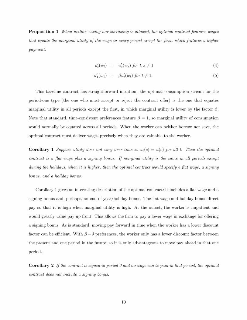
I.2 Pay Frequency

Table 1 indicates that the vast majority of states in the U.S. (45/51, including Washington D.C.)

explicitly regulate pay frequency. Only Alabama, Florida, Montana, Nebraska, Pennsylvania, and

South Carolina lack standards specifying the minimum time between paychecks. As the totals

indicate, approximately half of states specify a semi-monthly (or bi-weekly) frequency, with half

again requiring pay at the monthly frequency. Weekly pay, the highest frequency we observe, is

mandated in six states. As our analysis of the model below shows, the bene�ts of pay frequency

are larger for less wealthy workers, i.e., those who live �paycheck to paycheck.�Indeed, inspection

of state regulations reveals a number of cases where low wage jobs are singled out� even within

the same state� as requiring higher frequency. For instance, �executive� (in District of Columbia

and Georgia) and �professional�(in Illinois and Maryland) jobs are often exempted from the rules,

or subject to less stringent frequency requirements. As a more speci�c example, the New York

Labor Law (Section 191� Frequency of Payments) spells out di¤erent pay frequencies for 1) manual

and/or railroad workers, paid at least weekly, 2) clerical workers, paid at least semi-monthly, and

3) commission salesman, paid at least monthly.

Aggregate data on pay frequency, obtained from the U.S. Census Bureau Survey of Income and

Program Participation (1996), con�rms a similar pattern. Figure 3 shows that pay frequency is

monotonically related to monthly income, with workers paid monthly earning approximately 45%

more than workers paid weekly. Likewise, Figure 1 shows pay frequency for two alternative measures

of wealth and/or �nancial sophistication, �some stock ownership� or �some certi�cate of deposit

(CD) ownership.�Perhaps not surprisingly, the results here mimic those in the previous �gure, with

higher pay frequency associated with lower rates of �nancial market participation.

Our theory shows that more present-biased workers should be paid more frequently. Although

present-bias is di¢ cult to observe directly, there are good reasons to think it correlates with ed-

ucational attainment. Investing in education requires one to forgo immediate consumption, and

studying requires a postponement of immediate grati�cation. Individuals with present-bias are

therefore less likely to attain high levels of education. Figure 2 presents the cumulative distribution

7

of pay frequency by educational attainment. Over 20% of workers paid weekly lack a high school

diploma, versus only 6% of workers paid monthly. Moreover, for any level of educational attainment

X, a greater fraction of workers paid weekly have education less than or equal to X than workers

paid bi-weekly. The same follows for bi-weekly versus monthly.

I.3 Mechanisms Initiated by Workers

One of the theory�s key assumptions is that the appropriate timing of wage payments ultimately

bene�ts workers, and that workers are �sophisticated�enough to recognize the corresponding im-

provement in utility. Perfect sophistication is not required for the model�s implications to be rele-

vant, but support for the idea that workers are at least somewhat aware that pay timing can a¤ect

their long-run utility can be gleaned by examining their own, rather than their employers�, �nancial

decisions.

Workers sometimes choose to smooth pay that would otherwise vary in a way unrelated to

marginal utility. As an example familiar to academics, most U.S. universities and schools pay

salaries based on a nine month calendar year. Yet, many professors and teachers choose to spread

pay equally over twelve months, despite a loss of interest income. Likewise, utilities frequently o¤er

customers the option of paying equal amounts throughout the year, allowing them to better balance

their monthly expenditures. Workers also choose to convert smooth pay to pay that varies with

marginal utility, for example by requesting that an employer withhold more in tax than is expected

to be owed, thereby creating a type of savings account (also with a loss of interest). These savings

allow workers to save for large purchases such as a car (Adams, Einav and Levin, 2009). Certain

installment loans allow the borrower a �month o¤� at her discretion, presumably in a month in

which she has a high need for cash. In such a case, her net pay is higher when it is more needed.

II The Model

Our model is devoted to understanding the impact of time-inconsistency on contract design. Screen-

ing, signaling and motivating clearly play a role in contract design, and many papers have developed

theories of contracting that are designed to perform these three tasks. On the other hand, there are

many empirically common, but seemingly mundane, variations in contracts that are not well ex-

8

plained by these three more analyzed justi�cations. We show that many of these follow immediately

from workers�time-inconsistency.

To focus on precisely this driver of contract design, we model a setting in which there is neither

moral hazard nor adverse selection, and there is no risk in the productive technology. We begin

with a very narrow question: what is the optimal contract when the worker may neither borrow nor

save? We then allow the worker to save and show that our result does not depend on the no-saving

requirement. The results in these sections have a variety of implications for contract design which

are largely consistent with the stylized facts. We then turn to the question of how frequently workers

should be paid.

II.1 The optimal contract when no saving is allowed

A �rm must hire a worker for T periods and o¤er an initial present value of utility to the worker

of �u. Once hired, the worker will remain with the �rm throughout the duration of the contract:

there are no individual rationality constraints after the �rst (the contract is enforceable in court).6

The worker has period utility of ut(ct) where u has the standard properties: u0t(c) > 0; u00t (c) < 0;

and u0(0) = 1. Let the �rm pay a wage of wt. The �rm�s problem is to design a contract that

minimizes its expenses subject to the worker accepting the contract� it is assumed to be pro�table

at the optimal contract. Let the worker have � � � preferences with 0 < �; � � 1. That is, the

worker�s utility in period t is

Ut = ut(ct) + �

T�tXs=1

�sut+s(ct+s): (1)

Suppose the worker can neither borrow nor save. Then wt = ct, so the optimal contract satis�es

minfwtgt=1:::T

TXt=1

�t�1wt (2)

s:t: u1(w1) + �

TXt=2

�t�1ut(wt) � �u: (3)

6While this assumption is in violation of the 13th ammendment of the US constitution, it could be removed atthe expense of parsimony. Allowing the worker to quit at any time could change pay timing pro�les in which largepayments are made early in the life of the contract, but would not a¤ect those where larger payments are deferred.For example, workers starting a job in November might not be granted a Christmas bonus, but workers starting inFebruary would. It is empirically common, in fact, for bonuses to have such a pro-rating provision. If we assume apositive separation cost, then we would �nd that higher separation costs allow more front-loaded contracts.

9

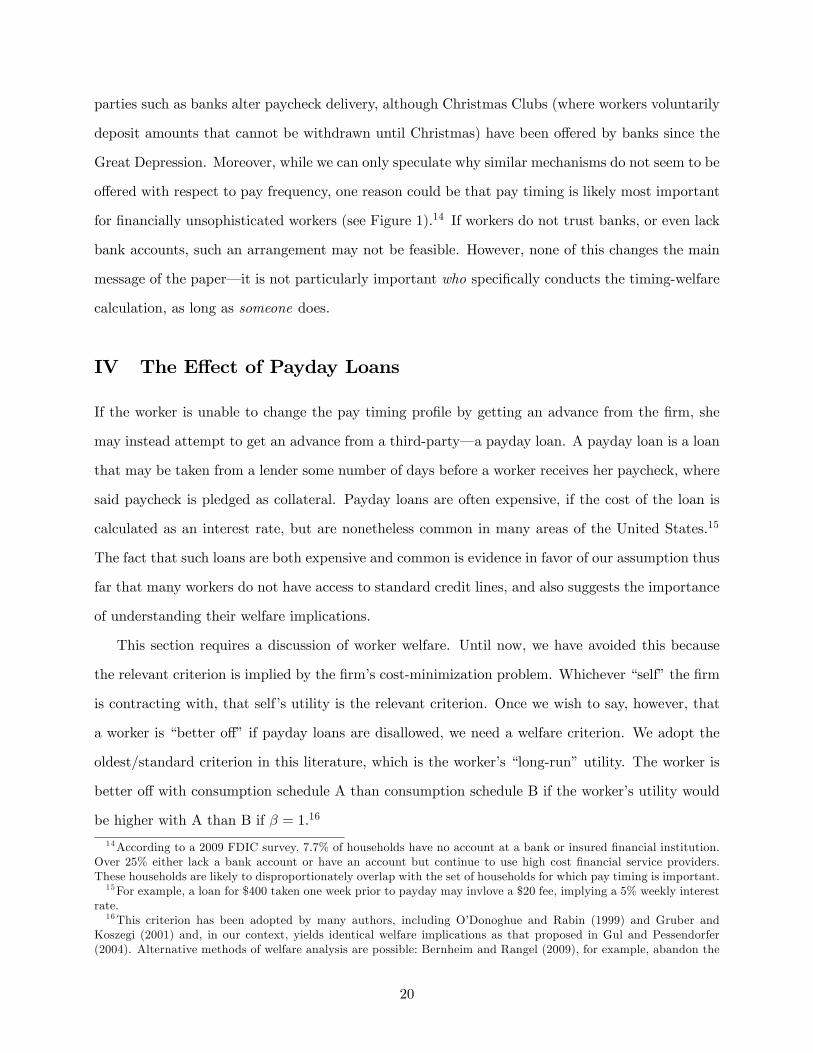
Proposition 1 When neither saving nor borrowing is allowed, the optimal contract features wages

that equate the marginal utility of the wage in every period except the �rst, which features a higher

payment:

u0t(wt) = u0s(ws) for t; s 6= 1 (4)

u01(w1) = �u0t(wt) for t 6= 1: (5)

This baseline contract has straightforward intuition: the optimal consumption stream for the

period-one type (the one who must accept or reject the contract o¤er) is the one that equates

marginal utility in all periods except the �rst, in which marginal utility is lower by the factor �.

Note that standard, time-consistent preferences feature � = 1, so marginal utility of consumption

would normally be equated across all periods. When the worker can neither borrow nor save, the

optimal contract must deliver wages precisely when they are valuable to the worker.

Corollary 1 Suppose utility does not vary over time so ut(c) = u(c) for all t. Then the optimal

contract is a �at wage plus a signing bonus. If marginal utility is the same in all periods except

during the holidays, when it is higher, then the optimal contract would specify a �at wage, a signing

bonus, and a holiday bonus.

Corollary 1 gives an interesting description of the optimal contract: it includes a �at wage and a

signing bonus and, perhaps, an end-of-year/holiday bonus. The �at wage and holiday bonus direct

pay so that it is high when marginal utility is high. At the outset, the worker is impatient and

would greatly value pay up front. This allows the �rm to pay a lower wage in exchange for o¤ering

a signing bonus. As is standard, moving pay forward in time when the worker has a lower discount

factor can be e¢ cient. With �� � preferences, the worker only has a lower discount factor between

the present and one period in the future, so it is only advantageous to move pay ahead in that one

period.

Corollary 2 If the contract is signed in period 0 and no wage can be paid in that period, the optimal

contract does not include a signing bonus.

10

If the contract is signed well before the worker joins the �rm, a payment at signing may not be

possible, or at least might not apply to the worker�s initial individual rationality constraint.7 In

this case, we should expect no signing bonus since the worker�s period zero discount factor between

period one and two is �, equal to the �rm�s.

II.2 The optimal contract when saving is allowed

If saving is allowed, the previous contract remains optimal because the present-biased worker will

never choose to save. Of course, if the worker has time-consistent preferences and can save at

interest rate r = 1� � 1, the previous contract is only one example of an optimal contract. Any

contract that speci�es payments that have the same cumulative total as the preceding contract at

every time t is equivalent. To see this, let fw�t gt=1:::T be the wage schedule in the �rst-best contract

and let R = 1 + r be the interest factor. Let �wt =Pts=1R

t�sw�s be the value at time t of wages

paid in the �rst-best contract up to time t. Then any contract fw0tgt=1:::T wherePts=1R

t�sw0s � �wt

for all t is equivalent for the worker. She can always save to replicate the �rst-best contract. For

example, the contract could o¤er the entire wage in period one so that w01 =PTs=1 �

s�1w�s and

w0t = 0 for t 6= 1, and allow the worker to save.

The case where � = 1, with a collection of equivalent contracts, is a knife-edge case. When

� < 1 the worker will not save su¢ ciently, and the more that the contract requires saving, the less

value she will get from the contract. To see that the �rst best contract, described in Proposition 1,

is uniquely optimal, consider a small deviation in which the worker is paid one extra dollar in period

t and 1� dollars less in period t+ 1. These contracts would normally be equivalent since, in theory,

the worker could save the dollar and match the previous consumption schedule, which is optimal for

the time-zero worker. When � < 1, however, the worker in period zero realizes that her period t self

will consume, rather than save, the dollar. After all, her period t self has a discount factor for period

t to any future period that is strictly between � and ��, so she would like to choose consumption

in the two periods so that u0t(ct) < u0t+1(ct+1). Since the �rst-best contract sets u

0t(ct) = u

0t+s(ct+s),

her period t marginal bene�t from shifting consumption from t + s to t is greater than unity: she

will consume a dollar delivered early. Her period zero self has discount factor � between the two

periods, and is therefore less happy with the consumption stream that will ensue if the contract

7See Van Wesep (2010) for a more detailed discussion of this issue.

11

pays money earlier. When employees are time-inconsistent, they are only able to e¢ ciently save if

the contract saves for them.

Note that this implies that this contract should be o¤ered to all of a �rm�s employees, regardless

of the distribution of � among them. Employees that are not present biased are not harmed by this

pay schedule, and those that are present biased are strictly helped. It is therefore easy for a �rm

that does not know the degree to which present-bias is prevalent among its workers to choose an

optimal contract.

II.3 The Frequency of Pay

The benchmark analysis so far has shown that pay, when delivered to coincide with periods of high

marginal utility, will reduce the �rm�s overall wage costs. We have been intentionally agnostic,

however, about what constitutes a �pay period�as, indeed, the model suggests that the �rm would

pay the worker continuously. This is clearly unrealistic� in practice, on the vast majority of days,

workers are paid nothing. To accommodate this feature and increase the realism of the model, we

now incorporate a cost each time the worker is paid. As we will see, this feature delivers optimal

pay frequency as balancing the physical costs of paying more often and the welfare bene�ts derived

in the last section.8 Moreover, the model can now also speak to the types of workers we expect to

be paid more or less frequently.

Let the cost of making a wage payment in a given period be c > 0. This is a reduced form way

to state that higher frequency is costly for some reason, whether it be lost interest on the �oat,

administrative costs, un-modeled moral hazard or screening costs, etc.9 For simplicity, assume that

8The optimality of periodic pay here derives from a similar trade-o¤ as is found in Clower constrained models (e.g.,Clower 1967; Lucas, 1980) in which consumption must be funded with cash, which may only be transferred from asavings account at a positive �xed cost. In these models, withdrawals from savings occur at �xed, periodic intervals.Huberman (1988) provides a theoretical foundation for the use of periodic actions/transactions even when the bene�tsor costs of action are stochastic. We therefore believe that our conclusions regarding optimal pay frequency do notdepend heavily on our assumptions of periodic pay and determinism.

9To delve more deeply in what such a cost may be, let us consider administrative costs of paying workers. Inorder for paychecks to be sent out, an employee of the �rm must check that the bank account from which the checkswill draw has su¢ cient funds. If funds are unavailable, other cash must be transferred into the account. If no othercash is available, some assets must be liquidated. This may require e¤ort from a CFO or some higher authority. Ifaccounts receivable become cash in a less-than-predictable way, then this process may be fairly costly. Regardless ofthe precise mechanism that causes paying workers to be costly, and regardless of whether the particular process wedescribe is accurate at every �rm, it should be clear that there is some cost of more frequent paychecks. As evidencethat the cost of making wage payments includes a �xed cost, and is not solely proportional to the number of workers,note that �rms o¤ering pay to some workers on a monthly basis also tend to o¤er pay to less educated workers on asemi-monthly, rather than bi-weekly, basis. Firms that pay some workers weekly tend to pay others bi-weekly, notsemi-monthly. This practice minimizes the number of days per month on which at least one wage payment is made,

12

the contract is signed in period zero and payments begin in period one, and let ut = u for all t. We

look for contracts with periodic payments: payment every period, every two, every three, etc.

Clearly, the optimal contract when � = 1 is to pay the full present value of the contract at the

outset. There is only one costly wage payment and the worker can save to smooth consumption

herself. Her consumption from a contract paying one payment in period one is shown in Figure

4. As we can see, as � decreases, the problem of over-consumption early in the contract becomes

increasingly severe. Therefore, � = 1 is a knife-edge case: for any � < 1, payments should be

periodic. As � declines, the worker is less able to save e¢ ciently and therefore bene�ts from more

frequent payment.

Suppose that payments are made every F 2 F periods, where F = f1; 2; :::; Fg[T and T = F !.

This assumption will ensure that F divides T for all possible F under consideration.10 Then the

worker must save for F � 1 periods with the wage payment in the �rst. Let wF be the payment

made every F periods and let si be the amount saved entering period i within the pay-period. That

is, s1 is the worker�s savings at the start of in the period in which she is paid, s2 is her savings

at the start of the next period, etc., and sF equals the savings in the ultimate period before she

is paid again. To see how valuable a contract with frequency F is to a worker, we can calculate

her consumption in each of the F periods between payments. The problem is identical after each

payment since T is a multiple of F .

We derive our results below using backward induction from the date before the next paycheck,

but a brief application of previous �� � results to our setting is useful. Harris and Laibson (2001)�s

Hyperbolic Euler Relation, adapted to the model at hand, can be written as

u0(cF�i�1)

u0(cF�i)= 1� (1� �)dcF�i

dsF�i; (6)

where dcF�idsF�i

is the fraction of the marginal saved dollar that is applied to consumption in the

following period. Because dcF�idsF�i

> 0, u0(cF�i�1)u0(cF�i)

is less than unity, consumption is decreasing over

time within a pay-period. Since the worker will not save in the period before a new paycheck,11

suggesting some �xed cost.10We will sometimes refer to F as the �pay frequency.�While the frequency is literally 1=F , we simply refer to it

as F for readability. �Higher frequency�corresponds to a lower value of F .11As we will see, the worker�s marginal utility in the period preceding a paycheck is greater than in that following

a paycheck, so zero saving is optimal. That is, the consumer is at a corner solution of Equation (8) in Harris andLaibson (2001).

13

dcFdsF

= 1. Equation (6) can also be written iteratively as

u0(cF�i) = u0(cF )�

iYj=1

�1� (1� �) dcF�j

dsF � j

�: (7)

While this equation shows relative consumption, the budget constraint can pin down levels:

F�1Xi=0

�icF�i = wF: (8)

Note that as the length of the pay-period F increases, because u0 is decreasing, the level of con-

sumption at the beginning of a pay-period is increasing in F and the level of consumption at the

end is decreasing.

We henceforth make two simplifying assumptions. First, we set � = 1 to simplify the analysis.

Given that T is �nite, the qualitative results are not dependent upon � so long as it is positive.

Setting � = 1 is useful so that we can talk simply about �weekly pay�etc. without being concerned

with discount and interest rates.12 Second, we let u(c) = log(c) so that we can �nd analytical

solutions for the consumer�s problem. We believe, though we clearly cannot make an exhaustive

search, that most concave utility functions would deliver similar qualitative results.

Proposition 2 Consumption in period i of a pay-period of length F is given by

c1 = w � F

1 + (F � 1)� (9)

ci = w � F

1 + (F � i)� �

24i�1Yj=1

(F � j)�1 + (F � j)�

35 for i 2 f2; 3; :::; Fg: (10)

Proof. The worker in period F � 1 will choose consumption to maxcF�1 log(cF�1) + � log(sF�1 �

cF�1); which yields cF�1 = 1� cF . In terms of savings at time F � 1, we get cF�1 =

11+� sF�1 and

cF =�1+� sF�1. In period F � 2 the worker�s problem is

maxcF�2�sF�2

�log(cF�2) + �

�log

�1

1 + �sF�1

�+ log

��

1 + �sF�1

���; (11)

12� = 1 is also approximately correct, since we are comparing pay frequencies on the order of weeks, and weeklydiscount factors are likely very close to unity.

14

which can be written maxcF�2�sF�2 [log(cF�2) +X + 2� log(sF�2 � cF�2)] ;where X = �(log(�) �

2 log(1+�)); which does not depend upon cF�2. This yields cF�2 = 11+2� sF�2; cF�1 =

2�1+2�

11+� sF�2

and cF =2�1+2�

�1+� sF�2. Assume that the worker consumes her entire savings in the period before

her next paycheck. We will con�rm that this assumption holds below. Then the savings at the time

of the paycheck is s0 = 0 and the initial payment is wF . Completing the iteration therefore yields

c1 =1

1+(F�1)�wF; c2 =(F�1)�1+(F�1)�

11+(F�2)�wF; c3 =

(F�1)�1+(F�1)�

(F�2)�1+(F�2)�

11+(F�3)�wF et cetera, up to

cF =(F�1)�1+(F�1)�

(F�2)�1+(F�2)� :::

�1+�wF . This can be written generally as

c1 =wF

1 + (F � 1)� (12)

ci =wF

1 + (F � i)� �

24i�1Yj=1

(F � j)�1 + (F � j)�

35 for i 2 f2; 3; :::; Fg: (13)

We now check that the worker would prefer to consume her entire savings in the period before a

paycheck. We begin with the period before the �nal paycheck. The worker�s marginal propensity

to consume in the period of her �nal paycheck is dc1ds1

= 11+(F�1)� , so Equation (7) implies that

the worker�s ideal ratio of marginal utility in the period before a paycheck to the next period is

1=cF1=c1

= 1�(1��) dc1ds1 , unless the worker is at a corner solution, in which casec1cF> 1�(1��) 1

1+(F�1)� .

Since c1 > cF , it immediately follows that c1cF> 1 � (1 � �) 1

1+(F�1)� , so the worker indeed prefers

to spend her entire savings in the period before her �nal paycheck. The same analysis applies to all

previous paychecks iteratively.

Corollary 3 The marginal propensity to consume in a period is decreasing in � and in the time to

the next paycheck. In the limit where � = 0, the marginal propensity to consume is one. In the limit

where � = 1 and the worker is time-consistent, the marginal propensity to consume is the inverse

of the number of periods before the next paycheck.

Proof. The derivative of cF�i with respect to sF�i is

dcF�idsF�i

=1

1 + i�; (14)

which is decreasing in � and i. Inserting � = 0 or � = 1 yields a marginal propensity to consume

of one or 11+i respectively.

15

Naturally, more time-inconsistent people, who have a lower value of �, have a higher marginal

propensity to consume. As � ! 0, consumption responds to saving one for one and future saving

is nil. When there is more time before the next paycheck, however, consumption responds less to

saving. Because every worker, even a time-inconsistent one, prefers smooth consumption, each must

save more when there is more time before the next paycheck. Essentially, since a time i self knows

that her medium-term self will overconsume relative to her time i preferences, she is more willing to

save so that her longer-term self has greater consumption. This bene�cence toward her longer-term

self is partly mitigated by her time-inconsistency, and consumption is always decreasing during a

pay-cycle. Note also that when � = 1, the standard result concerning the marginal propensity

to consume holds. If there are i periods remaining in the pay cycle, then a time-consistent worker

spreads a marginal dollar equally over those periods, and the current one, so the marginal propensity

to consume is 1=(1 + i).

The consumption choices described in Equation (10) are shown in Figure 5 for workers with

� = 0:9 and � = 0:7. The worker consumes the most on payday and consumes less each subsequent

week before the next paycheck. The di¤erence between consumption from the week before payday

to the week after is roughly 22% when � = 0:9. For � = 0:7, the problem becomes severe, with

consumption in the week before payday roughly half of consumption in the week after.

Two implications immediately follow from Proposition 2. First, since per-period pay is �xed at

w and utility is concave, the long-run utility over the pay-period is decreasing in F , where long-run

utility corresponds to what the worker�s utility would be if � were equal to one. Longer pay-periods

imply more varied consumption, which is utility destroying for the worker. Second, when workers

are more time-inconsistent (� is lower), the divergence between the high initial consumption and

low terminal consumption within a pay-period is larger.

Together, these imply that worker utility is decreasing as pay becomes less frequent, with the

reduction in utility being larger when � is lower. If the �rm wishes to reduce the frequency of pay

and still meet the worker�s individual rationality (IR) constraint, it must increase the per-period

wage. This trade-o¤ will lead to an optimal frequency. As � decreases, the optimal choice of F

decreases. Let bw(F; �) be the per-period wage that must be paid to a � type, given frequency F .This is de�ned by the worker IR constraint binding in period zero,13 �u = � � (T=F )�

PFt=1 u(ct),

13Recall that in this special case, we have allowed � = 1 which makes the exposition simple. There is no qualitative

16

where total consumption in each pay-period is given by the budget constraint (8) and relative

consumption is given by (7). Let � bw(F; �) = bw(F; �)� bw(F � 1; �). Proposition 2 implies that �bw is positive and decreasing in �. Therefore:Proposition 3 The optimal length of pay-period is increasing in �, with a limit of T as � ! 1.

To get a sense of magnitudes, Figure 6 shows the additional weekly wage that must be paid

as the pay-period lengthens for a time-consistent type as well as a time inconsistent type with

� = 0:7. As the pay-period lengthens from one week to four weeks, for example, a time inconsistent

worker must be paid an additional 4%. This may seem small, but if wages are large fraction of a

�rm�s cost, then 4% of wages would constitute a substantial fraction of pro�t margins. With more

time-inconsistent workers, the impact will be magni�ed.

A �rm may not know its workers� levels of � and even if it does, may wish to choose a pay

frequency so that all workers within a given job class have the same pay frequency even if there

is heterogeneity in the level of �. Nonetheless, proposition 3 provides clear guidance as to which

job classes should be paid more frequently. Suppose that the �rm can observe some attribute

of the worker �, which is provides some information regarding the worker�s likely value of �. In

particular, suppose that the value of � for a worker is a random variable with cumulative distribution

G(�; �); � 2 (0; 1]. Let � 2 (a; b) where �1 < a < b <1, and let G(�; �1) �rst order stochastically

dominate G(�; �2) if and only if �1 > �2. This implies that as � increases, the expected value of �

for the worker increases. Proposition 3 immediately implies the following corollary:

Corollary 4 The optimal length of pay-period is increasing in �.

Any observable worker attributes that are associated with present bias will cause the �rm to pay

the worker more frequently. In practice, this means that if the distribution of present-bias di¤ers

depending upon job class, we will expect �rms to vary pay frequencies by job class as well.

To summarize the results so far, pay should be timed so that workers receive pay precisely when

they desire consumption, thereby eliminating the need for them to save or borrow. If paying workers

entails a cost, then pay may be infrequent, but when workers are particularly present-biased, the

�rm must simply bear those costs and deliver pay frequently.

di¤erence if we allow � 2 (0; 1) so long as the interest rate is given by r = (1=�)� 1.

17

These results, however, are subject to an important caveat that, to this point, we have left

unmentioned. Once the timing of pay is set, the t > 0 worker has every incentive to attempt

to undo the pay schedule. In the next two sections we consider two ways that she may achieve

this. The �rst is to renegotiate with the �rm and get �an advance�on a future paycheck. Indeed,

renegotiation will cause our results thus far to unravel, implying a need for regulation. The second

is to get an advance from a third-party� a payday loan. Because this is ex ante harmful for the

worker as well, regulators can help workers by illegalizing payday lending. We show, however, that

an even better policy is to permit capped payday loans.

III Renegotiation and Regulation

Thus far we have assumed that the �rm and worker can commit to not renegotiate the contract after

it has been signed. This assumption has bite: the period-one worker has di¤erent time preferences

than the period zero worker and, given the contract terms we derive above, would be willing to

sacri�ce disproportionate future income to obtain an advance. Large and on-going �rms may be

able to establish and maintain reputations for refusing to renegotiate, thus decreasing future wage

bills, but for many smaller companies renegotiation may be too tempting to avoid. As we show in

this section, this fact suggests a role for regulation. A regulator, by mandating holiday bonuses,

certain pay frequencies, etc., can maximize social welfare and solve the renegotiation problem.

III.1 Renegotiation

We begin by deriving the optimal renegotiation-proof contract. As we will see, there is a set of such

contracts, all yielding identical consumption paths. The �rm essentially pays the full amount at the

outset, and the worker consumes from that bu¤er savings over T periods. Equivalent contracts pay

the worker some cash later, but always deliver su¢ cient cash by each period so that this consumption

path is feasible.

Proposition 4 There are a continuum of optimal renegotiation-proof contracts, each inducing the

same consumption path as a contract o¤ering all pay in period one.

With renegotiation, the worker and �rm both know that when a future present-biased version

of the worker requests an advance, there will be an interest rate such that the �rm will accede.

18

A renegotiation-proof contract must therefore be designed so that the worker never asks for an

advance, implying that the worker�s consumption stream with any renegotiation-proof contract is

identical to that which obtains when the worker is simply paid the full amount up-front. Note that

this argument follows for holiday bonuses and any other compensation that is deferred so that the

worker has money when it is more needed.

III.2 Regulation

The above analysis implies that both the �rm and the worker would prefer, at time zero, for

an outside entity to prevent renegotiation of contracts. In practice, this is a government, and the

enforcement is not against renegotiation per se, but in favor of requiring disbursements at particular

times. Not surprisingly, the contract required by the regulator would be identical to those we have

already derived as the optimal contract for the �rm, under the assumption that it could commit.

This is because the social planner�s problem and the �rm�s problem are identical, up to a constant.

The regulator would trade o¤ the cost to a �rm of paying more frequently with the bene�t to a

worker of being paid more frequently. The regulator could not observe how present-biased each

individual is, of course, but could perhaps form estimates based upon observables (e.g., worker

education or job class). Indeed, as we have discussed, regulators in 45 US states require wages to

be paid at a minimum frequency that typically depends upon job class. Jobs that typically require

more education or �nancial savvy, or that are higher paid, require less frequent pay.

III.3 Firms vs. Financial Intermediaries in Timing Pay

A question that may arise is why �rms, per se, should be the ones to adjust the worker�s pay

timing. One could imagine, for example, banks or payday loan companies o¤ering a similar service.

Perhaps workers would make deposits at the beginning of a pay-period and then receive periodic

disbursements to correlate with rent, bills, or other expenditures. Such a third-party arrangement

may be bene�cial for a number of reasons, including �nancial institutions having lower transaction

costs, or perhaps possessing a reputation for being hard-nosed (non) renegotiators.

There is nothing in the model that prevents external parties from stepping in and, indeed,

because payroll services are often outsourced (especially for medium and small companies), this

might be happening to some degree in practice. We are not aware of any cases where true third

19

parties such as banks alter paycheck delivery, although Christmas Clubs (where workers voluntarily

deposit amounts that cannot be withdrawn until Christmas) have been o¤ered by banks since the

Great Depression. Moreover, while we can only speculate why similar mechanisms do not seem to be

o¤ered with respect to pay frequency, one reason could be that pay timing is likely most important

for �nancially unsophisticated workers (see Figure 1).14 If workers do not trust banks, or even lack

bank accounts, such an arrangement may not be feasible. However, none of this changes the main

message of the paper� it is not particularly important who speci�cally conducts the timing-welfare

calculation, as long as someone does.

IV The E¤ect of Payday Loans

If the worker is unable to change the pay timing pro�le by getting an advance from the �rm, she

may instead attempt to get an advance from a third-party� a payday loan. A payday loan is a loan

that may be taken from a lender some number of days before a worker receives her paycheck, where

said paycheck is pledged as collateral. Payday loans are often expensive, if the cost of the loan is

calculated as an interest rate, but are nonetheless common in many areas of the United States.15

The fact that such loans are both expensive and common is evidence in favor of our assumption thus

far that many workers do not have access to standard credit lines, and also suggests the importance

of understanding their welfare implications.

This section requires a discussion of worker welfare. Until now, we have avoided this because

the relevant criterion is implied by the �rm�s cost-minimization problem. Whichever �self�the �rm

is contracting with, that self�s utility is the relevant criterion. Once we wish to say, however, that

a worker is �better o¤� if payday loans are disallowed, we need a welfare criterion. We adopt the

oldest/standard criterion in this literature, which is the worker�s �long-run�utility. The worker is

better o¤ with consumption schedule A than consumption schedule B if the worker�s utility would

be higher with A than B if � = 1.16

14According to a 2009 FDIC survey, 7.7% of households have no account at a bank or insured �nancial institution.Over 25% either lack a bank account or have an account but continue to use high cost �nancial service providers.These households are likely to disproportionately overlap with the set of households for which pay timing is important.15For example, a loan for $400 taken one week prior to payday may invlove a $20 fee, implying a 5% weekly interest

rate.16This criterion has been adopted by many authors, including O�Donoghue and Rabin (1999) and Gruber and

Koszegi (2001) and, in our context, yields identical welfare implications as that proposed in Gul and Pessendorfer(2004). Alternative methods of welfare analysis are possible: Bernheim and Rangel (2009), for example, abandon the

20

We begin by considering the case where payday loans are uncapped, meaning that the maximum

loan value is equal to the size of the paycheck. We restrict attention to the case where a loan may be

taken out one period before payday, though most of our policy prescriptions have clear analogues in

the more general case.17 Let the interest rate on payday loans be r 2 [0; 1��� ) and de�ne R = 11+r :

IV.1 Uncapped payday loans and welfare

If F = 1 and pay is every period then payday loans are identical to credit cards with a debt ceiling

equal to the size of the paycheck. We therefore focus, in this section, on the case where F � 2.

Proposition 5 When payday loans are uncapped and paychecks are infrequent, F � 2, the avail-

ability of payday debt shifts the consumption cycle forward by one period, increasing consumption

in the �rst F periods and decreasing it in the �nal F periods. Speci�cally, in all but the �nal period

of each pay-period, the worker�s consumption:

1. In the �rst F � 1 periods is identical to what would obtain without payday lending and with

paychecks of size wF but pay periods of length F � 1.

2. In the �nal F + 1 periods is identical to what would obtain without payday lending and with

paychecks of size wF but pay periods of length F + 1.

3. In the periods between is identical to the case without payday lending, but shifted one period

earlier.

In the �nal period of each pay-period, consumption is R times what obtains when payday loans

are not available.

Figure 7 shows the consumption cycle described in Proposition 5, with r = 0; F = 4 and � = 0:7.

For the bulk of the contract term, the consumption pattern is identical to the case with no payday

lending, but shifted forward by one period. The worker knows that her future self will take a

large payday loan, so will consume her entire paycheck a period earlier than when no payday loans

are available. Payday lending therefore simply shifts consumption forward one period. This raises

concept of preferences entirely, but also provide a choice-theoretic ground for the long-run criterion.17 In practice, payday loans can often be taken out by consumers two or more weeks before the next paycheck. We

do not precisely connect the concept of a �period" in this model to weeks or days in the real world. We could easilychange the allowable types of payday loan, but the qualitative trade-o¤s we analyze here would remain.

21

consumption somewhat at the start of the contract and decreases it somewhat at the end. From

the perspective of the period-one worker, payday lending could be bene�cial since consumption is

higher in period one, but the overall welfare e¤ect is small.

From the perspective of the period-zero worker, when r = 0 , payday lending is harmful because

consumption is slightly less even, but this e¤ect is small as well. Payday lending is essentially

irrelevant when pay is infrequent, interest rates are low, and loans can be as large as a paycheck.

As interest rates increase, the worker is unambiguously worse o¤. Consumption in most periods

is unchanged as r increases, but consumption in the period in which the payday loan is taken out

decreases with no corresponding increase elsewhere.

Corollary 5 As the interest rate on payday loans increases, consumption in the period before payday

decreases so that the amount repaid remains constant. Consumption in other periods of the pay-

period is una¤ected.

IV.2 Capped payday loans and welfare

Payday loans can, however, be bene�cial when the size of the payday loan is capped at an amount

less than the worker would like to borrow.

Proposition 6 Payday lending can improve long-run utility if the loan amount is capped. The

optimal cap is either 0 or T�F1+T�FRw, which is approximately equal to Rw when T is large.

Figure 8 shows the consumption pattern for three representative levels of the cap, assuming

r = 0. There are two e¤ects on consumption when the cap is increased. First, some consumption

is shifted from the �nal F periods of the contract to the �rst F � 1. This is a negative e¤ect of a

higher cap. Second, the variance in consumption in the middle periods of the contract decreases as

the cap approaches w and increases again for higher values of the cap. Therefore, welfare in the

middle periods of the contract is concave in the level of the cap, attaining a maximum when the

cap is w. The optimal value of the cap trades o¤ these e¤ects. Because T is large compared to F ,

the �rst e¤ect is small relative to the second, yielding an optimal cap close to w. As T ! 1, the

optimal cap tends to w.

To see why long-run utility is concave in the size of the cap, we must consider how the cap

a¤ects consumption during the pay-cycle. When the cap is low, increasing the cap does not a¤ect

22

the consumption cycle in the middle of the contract. Consider a typical pay-period and a cap C.

The worker will have borrowed C before the pay-period, and will also have access to a payday loan

of size C in the �nal period of the pay-period. Her cash available for consumption in the pay-period

is therefore wF � C + C = wF . Her options are unchanged, so her behavior is unchanged. We

see that for a cap of both 20% of weekly pay and 60% of weekly pay, her consumption cycle in the

middle of the contract is identical.

If the cap gets large, however, things are somewhat di¤erent. She begins the pay-period with

wF � C and knows that she will borrow C in the �nal period of the pay-period. By spreading

wF � C over F � 1 periods, she consumes less than C=� in the penultimate period of the pay-

period. She would like to increase consumption in the penultimate period and reduce it in the �nal

period, but she cannot access the payday loan until that �nal period. Therefore, she spreads her

paycheck, net of the cap, over F � 1 periods, knowing that in the �nal period of the pay-period she

will again borrow C. The payday loan e¤ectively changes the wage stream from one payment of wF

every F periods to a payment of wF �C that must cover F � 1 periods, and a payment of C every

F periods, just prior to the paycheck.

When the cap equals w, increasing the cap would increase her consumption in the period before

a paycheck, but this would raise her consumption that period to a level higher than her average

consumption in other periods, and therefore would reduce welfare. Another way to view the e¤ect

of a payday loan cap is shown in Figure 9. This �gure plots consumption in the �rst, second, third

and fourth periods of a contract with F = 4 for a worker with � = 0:7. These are consumption

levels in the middle of a contract: we ignore here the e¤ect of the payday lending cap on the �rst

and last pay-periods. We see that when the cap is small, there is no e¤ect on consumption. Only

when the cap is so large that the worker in period 3 of a pay-period would like to borrow does the

consumption change as we adjust the cap. Then, consumption in the period before payday begins

to rise and consumption in the other periods begins to fall.18 Eventually, the cap is large enough

that it does not bind.18There is a small bump in the consumption curves when the �no borrowing except before payday�constraint binds.

This is because the worker saves early in the pay-period, knowing that her self at the end of the pay-period will receivesome of that savings. Once the constraint binds, her saving will be consumed earlier and her discount rate is thereforehigher, reducing saving and increasing consumption. This also accounts for the small negative hit to average utilitywhen the cap is 0.7, shown in Figure 10.

23

We can see that the consumption over four periods is the same as with no payday lending or a

small cap, but with the highest consumption immediately before payday and lower consumption in

subsequent periods. The variation in consumption is clearly lowest when the cap equals per-period

pay.

Long-run utility as a function of the cap is plotted in Figure 10 for three types of contract. For

lower levels of �, consumption during a pay-period is less smooth, so capped payday loans are more

bene�cial. For longer-term contracts, payday loans are more bene�cial as well. This is because

the bene�t of smoother consumption in the middle cycles of the contract occurs for a longer time

and is therefore more able to o¤set the cost of shifting consumption from the end to the start of

the contract. Note also that as F increases, consumption is more volatile within a pay-period, so

capped payday loans are more bene�cial for the worker.

If we allow the interest rate r to increase, then payday lending is less valuable for the worker.

Her self in period F of each pay-period will continue to take out payday loans, at the expense of her

long-run self. While the shape of long-run utility as a function of the cap is the same as in Figure

10, the peak is at a lower cap as we increase r. Interestingly, while the optimal cap decreases as the

interest rate on payday loans increases, the repayment amount is approximately w regardless of the

interest rate.

IV.3 Implications for payday lending policy

To summarize the implications from this section, payday loans can be either good or bad, depending

on when the consumer accesses them, and how much she is allowed to borrow. First, we have found

that payday loans improve welfare when their use is restricted to times when consumption is very

low, which, in our model occurs: 1) at the end of the pay cycle, and 2) when paychecks arrive

infrequently. Second, we have shown that granting unlimited access to payday loans does nothing

to smooth consumption� in fact, it delivers the opposite result� but that limiting access to periods

directly before a paycheck and capping the loan amount can produce welfare improvements.

This dual prediction is useful in both a descriptive and prescriptive sense. Descriptively, it

is noteworthy that a consensus on the welfare impacts of payday lending is far from unanimous,

both within and outside of academia. As of the writing of this manuscript, a bill sponsored by

North Carolina Senator Kay Hagan (D) would place federal restrictions on payday amounts. �By

24

reigning in payday lenders, we will protect consumers from racking up endless, long-term debt that

can ultimately cause a family to declare bankruptcy,� she said.19 Her position is buttressed by a

number of academic studies that document negative welfare e¤ects for users of payday loans. For

example, Skiba and Tobacman (2009) �nd that even though the average payday loan amount is

small (around $300), borrowers were substantially more likely to declare personal bankruptcy in

the months following a loan. Likewise, Melzer (2009) �nds that payday borrowers experience a

wide variety of negative welfare-reducing events: increased likelihood of being late on bill payments,

delaying medical care, forgoing the �lling of prescriptions, etc.

On the other hand, the selection issues surrounding payday lending are considerable: because

consumers are not randomly selected to have access to loans, nor to borrow, the possibility that

payday loans are simply a proxy for (imperfectly observed) �nancial distress is concerning. Indeed,

some empirical studies have documented positive e¤ects of payday lending. For example, Morse

(2009) examines payday loans within California from 1996-2002, �nding that �payday loan commu-

nities�were less impacted by natural disasters than those lacking such establishments. A natural

reconciliation of these �ndings� and one to which our analysis directly speaks� is that payday loans

help consumers, provided that they are used for the right purposes. In Morse�s study of natural

disasters, payday loans are used in presumed states of (very) high marginal utility; more generally,

payday loans may facilitate consumption in less dire situations. Our study suggests exactly this,

although what constitutes an appropriate use of payday lending can be summarized by when it is

accessed during the pay cycle.

Together, this analysis suggests a clear policy implication: payday loans and similar instruments

are bene�cial only when the loan amount is capped, and are particularly bene�cial at the end of the

pay cycle. However, actual policy appears to re�ects only this �rst implication. As shown in the �nal

three columns of Table 1, when payday loans are allowed, they are usually capped, both in term and

amount. However, these limits appear to bear little systematic relation to pay frequency, which the

theory indicates should be closely connected. Speci�cally, the theory indicates that payday loans

strictly decrease welfare if workers can access them too early in the pay cycle. This will of course be

the case if payday loan terms are longer than the pay cycle, allowing workers to perpetually access

payday loans, rather than only immediately preceding a paycheck.

19See http://hagan.senate.gov/?p=press_release&id=551.

25

The vast majority of states (41), however, allow the term of a payday loan to span an entire pay

cycle. As a particularly egregious example, Vermont requires workers to be paid weekly (and within

six days of the end of a pay-period), but payday lending remains virtually unregulated, both in term

and amount. The model predicts that in such a case, workers simply access the maximum amount

they are permitted as early as possible, and experience lower consumption over their lifetimes. The

prohibition of payday lending in Massachusetts, a state that also mandates frequent (weekly) pay,

is more consistent with the theory, but this is the exception rather than the rule. In light of our

analysis, this is a puzzling �nding, and could perhaps shed light on the con�icting �ndings for the

welfare e¤ects of payday lending discussed above. When pay is delivered frequently to employees,

payday lending can have little other e¤ect than to encourage perpetual indebtedness, rather than

to deliver consumption near the end of the pay cycle. A cross-sectional analysis of payday lending�s

e¤ects on welfare, particularly as it relates to pay frequency laws, would buttress support for the

resulting policy implications.

V Could alternative assumptions concerning behavior generate

our results?

There are several assumptions we have made to get our results. We have assumed that the

worker is time-inconsistent and sophisticated, and we have assumed that workers are largely credit-

constrained. In this section we discuss which assumptions are necessary and which could be altered.

We discuss �rst the di¤erence between the optimal contract implied by time-inconsistency versus

that implied by impatience, in which the worker�s discount rate is higher than the �rm�s. Impa-

tience cannot generate our results. We then discuss the importance of sophistication in our model

and how we could change the model if the worker were naïve. We �nish by showing that credit

constraints for the worker are not, on their own, su¢ cient to generate the contractual implications

we derive above.

V.1 Time-inconsistency versus impatience

If the worker is simply impatient, rather than time-inconsistent, her discount factor, �w; is less

than the �rm�s discount factor, �F . She prefers to front-load consumption and the �rm is happy to

26

deliver. Because an impatient worker is not time-inconsistent, there are many contracts that deliver

the �rst-best consumption stream. One such contract would be the �rm simply giving a lump-sum

at the start of the contract. Our results are therefore clearly inconsistent with impatience alone.

With time-inconsistency, the �rm bene�ts by helping the worker help herself: the worker is willing

to accept a lower wage in order to have smoother future consumption.

V.2 Sophistication versus naïveté

The worker signing the contract is willing to accept a lower average wage in exchange for better

timed wages because her future self would not make the saving decisions that her current self would

prefer. This clearly requires the worker to be sophisticated in her knowledge of herself. That is,

she must know that her future self will make di¤erent consumption choices if given the option and

therefore value a contract that removes that option.20

One could imagine, however, a slightly di¤erent set-up that does not require worker sophisti-

cation, but where pay timing is still important. For example, suppose that the �rm knows that

the worker is time-inconsistent but that the worker does not. Suppose further that at the end of

a pay cycle, workers desperate for cash are poorly rested (e.g., from taking on extra work), poorly

nourished, or in some other way less productive. The �rm would then prefer a wage pro�le that

keeps the worker from experiencing periods of low consumption. That is, it may be productivity

improvements� not wage savings� that make timing important. We could construct a model in

which a �rm must hire a naïve worker and show an equivalent result to Proposition 1.

We therefore do not believe that our broader point� �rms employing time-inconsistent workers

must consider pay timing� is dependent upon the assumption of worker sophistication. We choose

in this paper to allow for sophisticated workers and to focus on wage savings from proper timing,

but allowing for naïveté would have been equally possible.

V.3 Credit constraints without time-inconsistency

It seems plausible that credit constraints alone could generate pay timing as we describe above.

Workers who live �paycheck to paycheck�would su¤er from infrequent pay since they would ex-

20 In a consumption-saving environment, Ali (2010) establishes a learning-theoretic basis for the assumption ofsophistication.

27

perience periods of very low consumption in the run-up to a paycheck. In fact, credit constraints

alone cannot generate our results. As we have shown, when � = 1, any wage schedule fw0tgt=1:::T

such thatPts=1R

t�sw0s � �wt is equally valuable for the worker. Paying the full amount due in the

contract up-front is as at least as good as any other mechanism. While the contract with a signing

bonus, holiday bonus, etc., is an example of a �rst-best contract, it is one of many.

We have shown that pay should be more frequent for more time-inconsistent workers, but this

also would not follow from credit constraints alone. One might argue the following: �Suppose it�s

two weeks before payday. If I were paid semi-monthly, then I would receive part of the check now

and part later. This would relieve a credit constraint since I�m poor now, and therefore increase my

utility.�But we must then ask why the worker is poor before payday. Indeed, on payday, a time-

consistent worker would be indi¤erent between a paycheck that pays the full amount immediately

or half now and half in two weeks. The problem of credit constraints only arises before the �rst

payment in a contract or because of time-inconsistency.

VI The optimal timing of government assistance

Foley (2009) �nds that crimes motivated by money are more frequent at the end of a welfare

payment cycle: as recipients run out of money over the course of the month, many turn to crime

to supplement income. Shapiro (2005) �nds that nourishment decreases over the month following

a welfare payment. Both results are consistent with recipients being time-inconsistent, and this

should be no surprise.21 A low value of � causes procrastination and an inability to put long-term

goals ahead of short term rewards, thus making it costly for time-inconsistent people to acquire an

education. A low value of � also makes them less able to show up for work on time, follow orders,

etc. The demand for current consumption, moreover, prevents the accumulation of wealth. The set

of people requiring government assistance is therefore likely to include a disproportionate number

possessing time-inconsistency.

Figure 5 shows how time-inconsistency can cause periods of severe under-consumption. The

welfare pay cycle in most states is monthly, implying that recipients with log utility and � =

0:7 consume only half as much in the week before payday as in the week after. This dearth of

21Both results are also consistent with impatience.

28

consumption could tempt some recipients to commit crime to supplement their meager savings in

these periods. Even if a recipient�s average utility over the course of the month is only roughly 4%

lower than if she were paid weekly, as is shown in Figure 6, her utility in the week before payday

is far lower because of her time-inconsistency. We do not model the decision to commit crime

explicitly, but it should be clear where the temptation arises.

The large majority of recipients of government assistance do not turn to crime, but they are

punished with low nourishment at the end of the pay cycle. Better designed welfare payments

could improve their livelihoods while reducing crime and saving taxpayer money. We argue that

a better system for government assistance would pay recipients when they need the money. A

social worker could work with the recipient to set out when large bills like rent and utilities are

due, for example, and these amounts would be directly deposited on the day the bills are due. The

remainder of the monthly stipend could be divided by the days in the month and deposited each day

into the recipient�s personal account. This would deliver money when it is needed and not require

the recipient to plan/save for an entire month. A plan that pays weekly, with bonus payments on

the day large bills are due, would probably do similarly well.

VII Conclusion

We develop a model of optimal pay timing for time-inconsistent workers. Because these workers have

di¢ culty saving, �rms pay them so that consuming the entire paycheck leads to constant marginal

utility over time: higher or lower pay coincides with periods of higher or lower marginal utility,

respectively. This can be implemented, for example, by a �xed wage plus a bonus for the holidays,

summer vacations, signing, or severance. We also analyze the case where paying more frequently is

costly, and show that time-inconsistent workers experience feast-famine consumption cycles within

a pay-period. When the time-inconsistency problem is more severe, the ex ante cost of these cycles

is also more severe, so pay should be more frequent. This is consistent with broad empirical patterns

we see in practice. Insofar as education and wealth correlate negatively with time-inconsistency,

more educated and more wealthy workers should be, and are, paid less frequently.

Given the optimal contract agreed-upon ex ante, the worker will attempt to undo the contract

ex post by either renegotiating the contract with the �rm or seeking a payday loan. We show that

29

the �rm will be happy to renegotiate, for a price, thus preventing the optimal contract from being

implemented. This suggests a role for regulators in which they require the �rm to pay workers

according to the optimal pay schedule. Indeed, regulation of holiday bonuses and pay frequency is

common both in the U.S. and internationally.

We also show that payday lenders will be happy to lend to the worker, though this fact can

be bene�cial or harmful. The worker�s consumption cycles can be at least partly mitigated with

payday loans, which deliver cash to the worker in periods when consumption would otherwise be

low, and remove cash in periods where consumption would otherwise be high. We show that this is

only the case when the amount of the payday loan is capped. Speci�cally, the maximum allowable

loan amount should equal the per-period pay multiplied by the number of periods before payday

when the money is borrowed. Essentially, payday loans are an inferior substitute for more frequent

pay: when pay is frequent, payday loans act as revolving debt and encourage life-long indebtedness.

When pay is infrequent, however, capped payday loans deliver money when it is most needed,

and can improve worker welfare. We provide prescriptive suggestions for legislation involving pay

frequency and consumer lending regulation.

We have attempted in this paper to provide a simple, parsimonious model in which many

features of contracts that we observe in practice result from a simple cost-minimization problem.

We do not consider issues of moral hazard or risk in the production process, nor do we address

the use of contracts to screen workers. In discussing policy implications for payday lending, we

do not model the broader planner�s problem. This is for three reasons. First, these additional

complexities are unnecessary for our results and would serve to make less clear the connection

between time-inconsistent preferences and pay timing. Second, as this paper is a �rst attempt

to tackle issues of pay timing, it is important to establish a baseline against which other results

can be compared. Third, working with time-inconsistent preferences quickly becomes analytically

infeasible as additional complexity is added. That said, extensions of the model are an area for

future work.

30

References

[1] Adams, William, Einav, Liran and Levin, Jonathan, 2011, �Liquidity Constraints and Imperfect

Information in Subprime Lending,�American Economic Review 99(1), 49-84

[2] Ainslie, George W., 1975, �Specious Reward: A Behavioral Theory of Impulsiveness and Im-

pulsive Control,�Psychological Bulletin, LXXXII, 463-96.

[3] Ainslie, George W., 1986, �Beyond Microeconomics. Con�ict among Interests in a Multiple Self

as a Determinant of Value.�in The Multiple Self, Jon Elster, ed. (Cambridge, UK: Cambridge

University Press).

[4] Ainslie, George W., 1992, �Picoeconomics�(Cambridge, UK: Cambridge University Press).

[5] Ali, Nageeb, 2011, �Learning Self-Control,�Quarterly Journal of Economics (forthcoming)

[6] Barro, R., 1999, Ramsey Meets Laibson in the Neoclassical Growth Model, Quarterly Journal

of Economics 114, pp. 1153-1191.

[7] Bernheim, D., Rangel, A., 2009, Beyond Revealed Preference: Choice-Theoretic Foundations

for Behavioral Welfare Economics, Quarterly Journal of Economics

[8] Clower, R., 1967, A Reconsideration of the Microfoundations of Monetary Theory, Western

Economic Journal, 6, pp. 1-8.

[9] Chung, Shin-Ho, and Richard J. Herrnstein, �Relative and Absolute Strengths of Response as

a Function of Frequency of Reinforcement,�Journal of the Experimental Analysis of Animal

Behavior, IV (1961), 267-72.

[10] Diamond, P. and B. Koszegi, 2003, Quasi-Hyperbolic Discounting and Retirement, Journal of

Public Economics Volume 87, Issues 9-10, 2003, Pages 1839-1872.

[11] Goldfarb, R., 1987. The Employer�s Choice of Paying Wages or Salaries, Proceedings of the For-

tieth Annual Meetings (Dec. 28�30). Madison, Wis.: Industrial Relations Research Association,

Vol. 40 (December), pp. 241�47.

[12] Gruber, J., Koszegi, B., 2001, Is Addiction �Rational�? Theory and Evidence, Quarterly

Journal of Economics 116(4), pp. 1261-1303.

31

[13] Gul, F., Pesendorfer, W., 2001, Temptation and Self-Control, Econometrica 69(6), pp. 1403-

1435.

[14] Gul, F., Pesendorfer, W. 2004, Self-Control, Revealed Preferences and Consumption Choice,

Review of Economic Dynamics, 7(2), pp. 243-264.

[15] Hayes, R. M. and Schaefer, S., 2009, CEO pay and the Lake Woebegone e¤ect, Journal of

Financial Economics 94, 280-290.

[16] Holmstrom, B., 1982, Managerial Incentive Problems - A Dynamic Perspective, in Essays in

Economics and Management in Honor of Lars Wahlbeck. Helsinki: Swedish School of Eco-

nomics, 1982.

[17] Fama, E., 1991, Time, Salary, and Incentive Payo¤s in Labor Contracts, Journal of Labor

Economics, Vol. 9, No. 1 (January), pp. 25�44.

[18] Foley, F., Welfare Payments and Crime, mimeo, 2009.

[19] Harris, C., Laibson, D., 2001, Dynamic Choices of Hyperbolic Consumers, Econometrica 69(4),

pp. 935-957.

[20] Huberman, G., 1988, Optimality of Periodicity, Review of Economic Studies 55(1), pp. 127-138.

[21] Laibson, D., 1997, Golden Eggs and Hyperbolic Discounting, Quarterly Journal of Economics

62, May, pp. 443-77

[22] Laibson, D., Reppeto, A., Tobacman, J., 1998, Self-Control and Saving for Retirement, Brook-

ings Papers in Economic Activity 1, pp. 91-196.

[23] Lazear, E., 2005. Output-Based Pay: Incentives, Retention, or Sorting? Research in Labor

Economics, 23, 1-25.

[24] Lazear, E., 1990, The Timing of Raises and Other Payments, Carnegie-Rochester Conference

Series on Public Policy, 33, pp. 13-48.

[25] Lazear, E., Rosen, S., 1981, Rank-Order Tournaments as Optimum Labor Contracts, Journal

of Political Economy 89, 5.

32

[26] Locas, R. 1980, Equilibrium in a Pure Currency Economy, Economic Inquiry, 18, pp. 203-220.

[27] Lusardi, A., Schneider, D. and Tufano, P. 2011, "Financially Fragile Households: Evidence and

Implications." Brookings Papers on Economic Activity, pp. 83-134.

[28] O�Donoghue, T. and M. Rabin, 1999, Doing it Now or Doing it Later, American Economic

Review 89, pp. 103-124.

[29] Melzer, B., 2009, The Real Costs of Credit Access: Evidence from the Payday Lending Market,

working paper.

[30] Morgan, D., Strain, M., �Payday Holiday: How Households Fare when States Ban Payday

Loans.�Working Paper, 2007.

[31] Morse, A., �Payday Lenders: Heroes or Villains?�forthcoming Journal of Financial Economics.

[32] McClure, S., Laibson, D., Loewenstein, G., and Cohen, J., 2004, �Separate Neural Systems

Value Immediate and Delayed Monetary Rewards,�Science, 136, 503-507.

[33] Parker, J., 1999, "The Reaction of Household Consumption to Predictable Changes in Social

Security Taxes," American Economic Review 89, 4, 959-73.

[34] Shapiro, Jesse, 2005, Is there a Daily Discount Rate? Evidence from the Food Stamp Nutrition

Cycle, Journal of Public Economics 89:2-3, pp. 303-325.

[35] Shapiro, C., and J. E. Stiglitz, 1984. Equilibrium unemployment as a worker discipline device.

American Economic Review 74, 433-444.

[36] Shea, J., 1995, Union Contracts and the Life-Cycle/Permanent-Income Hypothesis, American

Economic Review 85, 1, 186-200.

[37] Skiba, P., Tobacman, J., �The Pro�tability of Payday Loans,�Working Paper, 2009.

[38] Souleles, N., 1999, The Response of Household Consumption to Income Tax Refunds," Amer-

ican Economic Review 89, 4, 947-58.

[39] Stephens, M., 2003, ��3rd of the Month�: Do Social Security Recipients Smooth Consumption

Between Checks?�The American Economic Review, vol.93, n.1, p.406�422.

33

[40] Stephens, M., 2006, �Paycheque Receipt and the Timing of Consumption� The Economic

Journal, August 2006, vol. 116, issue 513, p.680�701

[41] Stephens, M., 2008, �The Consumption Response to Predictable Changes in Discretionary

Income: Evidence from the Repayment of Vehicle Loans�The Review of Economics and Sta-

tistics, vol.90, n.2, p.241-252

[42] Van Wesep, 2010, Pay (Be)fore Performance: The Signing Bonus as an Incentive Device, forth-

coming, Review of Financial Studies, 2010.

34

VIII Appendix

Proof of Proposition 1. The �rm�s problem can be written as the following Lagrangian

L = �TXt=1

�t�1wt + �

"u1(w1) + �

TXt=2

�t�1ut(wt)� �u#: (15)

The �rst order constraints are

1 = �u01(w1) (16)

1 = ��u0t(wt) for t = f2; 3; :::; Tg (17)

�u = u1(w1) + �TXt=2

�t�1ut(wt): (18)

Equation (17) yields u0t(wt) = u0s(ws) for t; s 6= 1 and combining Equations (16) and (17) yields

u01(w1) = �u0t(wt) for t 6= 1.

The following is a heuristic derivation of Equation (7), which follows closely to the derivation of

the Quasi-Hyperbolic Euler Relation in Harris and Laibson (2001). Consumption in period F � i

is chosen to maxc�sF�i�u(c) + ��UF�i+1(

1� (sF�i � c))

�, which yields the �rst order condition

u0(cF�i) = �U0F�i+1(sF�i+1): (19)

The marginal utility of consumption that period equals the marginal utility of saving, discounted

by �. Also,

UF�i(sF�i) = u(cF�i) + �UF�i+1(sF�i+1):

Marginal continuation utility can be found by taking a derivative of each side with respect to

sF�i:

U 0F�i(sF�i) = u0(cF�i)

�dcF�idsF�i

�+ �U 0F�i+1(sF�i+1)

�dsF�i+1dsF�i

�:

Since sF�i+1 = 1� (sF�i � cF�i) we can re-write this as

35

U 0F�i(sF�i) = u0(cF�i)dcF�idsF�i

+ U 0F�i+1(sF�i+1)

�1� dcF�i

dsF�i

�=

�u0(cF�i)� U 0F�i+1(sF�i+1)

� dcF�idsF�i

+ U 0F�i+1(sF�i+1)

= U 0F�i+1(sF�i+1)

�1� (1� �)dcF�i

dsF�i

�;

which implies

U 0F�i(sF�i)

U 0F�i+1(sF�i+1)= 1� (1� �)dcF�i

dsF�i:

Since dcF�idsF�i

< 0, marginal continuation utility is increasing in time since the last paycheck.

Plugging in u0(cF�i) = �U 0F�i+1(sF�i+1) yields

u0(cF�i�1)

u0(cF�i)= 1� (1� �)dcF�i

dsF�i:

Proof of Proposition 3. The per period wage, bw; multiplied by the number of periods perpay-period, F , is the size of the paycheck. c is the �xed cost of paying a check, so the total cost per

pay-period to the �rm is bw(F; �) � F + c. Since there are T=F pay periods, the �rm�s problem is

to choose F to

minF

T

F( bw(F; �)� F + c) :

Since bw is increasing in F and the rate of increase is decreasing in �, � bw is positive and

decreasing in �. This yields

@ bw(F; �)@F

F �2 = c

Since @ bw(F;�)@F is larger for lower �, the optimal time between paychecks F must be smaller. As

� ! 1, @ bw(F;�)@F ! 0 since the consumption choices speci�ed in Equation (7) do not vary with F . For

any positive c, therefore, F � ! 1 as � ! 1. The maximum allowable value of F is F , so F ! F

as � ! 1.

36

Proof of Proposition 2. The worker in period F � 1 will choose consumption to

maxcF�1

log(cF�1) + � log(sF�1 � cF�1);

which yields

cF�1 =1

�cF :

In terms of savings at time F � 1, we get

cF�1 =1

1 + �sF�1

cF =�

1 + �sF�1:

In period F � 2 the worker�s problem is

maxcF�2�sF�2

�log(cF�2) + �

�log

�1

1 + �sF�1

�+ log

��

1 + �sF�1

���;

which can be written

maxcF�2�sF�2

[log(cF�2) +X + 2� log(sF�2 � cF�2)]

where X = �(log(�)� 2 log(1 + �)); which does not depend upon cF�2. This yields

cF�2 =1

1 + 2�sF�2

cF�1 =2�

1 + 2�

1

1 + �sF�2

cF =2�

1 + 2�

�

1 + �sF�2:

Assume that the worker consumes her entire savings in the period before her next paycheck. We

will con�rm that this assumption holds below. When we iterate back to period 1, the savings at

37

the time of the paycheck is s0 = 0 and the initial payment is wF . Given F we have

c1 =1

1 + (F � 1)�wF

c2 =(F � 1)�

1 + (F � 1)�1

1 + (F � 2)�wF

c3 =(F � 1)�

1 + (F � 1)�(F � 2)�

1 + (F � 2)�1

1 + (F � 3)�wF

:::

cF =(F � 1)�

1 + (F � 1)�(F � 2)�

1 + (F � 2)� :::�

1 + �wF;

which can be written generally as

c1 =wF

1 + (F � 1)� (20)

ci =wF

1 + (F � i)� �

24i�1Yj=1

(F � j)�1 + (F � j)�

35 for i 2 f2; 3; :::; Fg: (21)

We now check that the worker would prefer to consume her entire savings in the period before a

paycheck. We begin with the period before the �nal paycheck. The worker�s marginal propensity

to consume in the period of her �nal paycheck is dc1ds1 =1

1+(F�1)� , so Equation (7) implies that the

worker�s ideal ratio of marginal consumption in the period before a paycheck to the next period is

1=cF1=c1

= 1� (1� �)dc1ds1

) c1cF= 1� (1� �) 1

1 + (F � 1)� ;

unless the worker is at a corner solution, in which case

c1cF> 1� (1� �) 1

1 + (F � 1)� :

Since c1 > cF , it immediately follows that c1cF> 1 � (1 � �) 1

1+(F�1)� , so the worker indeed prefers

to spend her entire savings in the period before her �nal paycheck. The same analysis applies to all

previous paychecks iteratively.

Proof of Proposition 3. The per period wage, bw; multiplied by the number of periods per38

pay-period, F , is the size of the paycheck. c is the �xed cost of paying a check, so the total cost per

pay-period to the �rm is bw(F; �) � F + c. Since there are approximately T=F pay periods,22 the

�rm�s problem is to choose F to

minF

T

F( bw(F; �)� F + c) :

Since bw is increasing in F and the rate of increase is decreasing in �, � bw is positive and

decreasing in �. This yields@ bw(F; �)@F

F �2 = c

Since @ bw(F;�)@F is larger for lower �, the optimal time between paychecks F must be smaller. As

� ! 1, @ bw(F;�)@F ! 0 since the consumption choices speci�ed in Equation (7) do not vary with F .

For any positive c, therefore, F � !1 as � ! 1.

Proof of Proposition 4.

We show the result using backward induction. Suppose the worker has savings of sT�1 entering

period T � 1 and is to be paid wT�1 that period and wT in the �nal period. The worker�s discount

factor between periods T � 1 and T is � < 1 whereas the �rm�s is unity. Suppose wTwT�1+sT�1

> �.

Then the worker would be willing to pay a positive interest rate to the �rm for an advance on the

�nal paycheck, and the �rm would be willing to accept a positive interest rate. Any contract where

this will result is therefore not renegotiation-proof. Therefore, wTwT�1+sT�1

� �. Regardless of the

wages and savings that allow that inequality to hold, consumption in the �nal two periods is given

by cTcT�1

= �. This argument follows iteratively for prior periods along lines shown in the proof of

proposition 2 and is therefore omitted here.

Proof of Proposition 5. Payday lending allows the worker to choose consumption in the period

before a paycheck just like every other period. Suppose that in the �nal period before her �nal

paycheck, she borrows B, so that B(1 + r) repaid when her �nal paycheck arrives. Then her

22�Approximately�, because T=F may not be intefer valued. The actual number of payments T=F rounded down.As T gets large, �xing F , the di¤erence between T=F and the actual number of pay-periods, as a proportion of totalcosts, goes to zero.

39

consumption in the �nal pay-period satis�es

c1 =wF �B(1 + r)1 + (F � 1)� (22)

ci =wF �B(1 + r)1 + (F � i)� �

i�1Yj=1

(F � j)�1 + (F � j)� for i 2 f2; 3; :::; Fg: (23)

Her borrowing choice is given by

B� = argmaxB

26664log(sF +B) + � log

�wF�B(1+r)1+(F�1)�

�+�

FXt=2

log

0@wF�B(1+r)1+(F�i)�

i�1Yj=1

(F�j)�1+(F�j)�

1A37775

= argmaxB[log(sF +B) + �F log (wF �B(1 + r))] :

Then borrowing equals

BT=F =RwF � �FsF1 + �F

;

where the superscript notes that it is the amount borrowed before the T=F (read: �nal) paycheck.

Her period F � 1 self (in the penultimate pay-period) must decide whether to save. We assume

she does not save, and con�rm this below. If she does not save, then cT=F�1F�1 = sT=F�1F�1 while her

next-period consumption equals BT=F = RwF1+�F . In the �nal pay cycle, when she will not be able to

take a payday loan at the end, her consumption is as before except with lower initial wealth (the

repayment amount of wF1+�F must be repaid at the start of the pay cycle):

cT=F1 =

�F

1 + �F

wF

1 + (F � 1)� (24)

=wF

1 + (F � 1)� �0Yj=0

(F � j)�1 + (F � j)� (25)

cT=Fi =

wF

1 + (F � i)� �

24i�1Yj=0

(F � j)�1 + (F � j)�

35 for i 2 f2; 3; :::; Fg: (26)

In the second through T=F � 1 cycles, her consumption is identical to the case without payday

lending, but the cycle begins one period earlier (the proof follows immediately from the proofs thus

40

far shown).

ck1 =(F � 1)�

1 + (F � 1)�wF

1 + (F � 2)� (27)

cki =wF

1 + (F � i)� �

24i�1Yj=1

(F � 1� j)�1 + (F � 1� j)�

35 for i 2 f2; 3; :::; F � 1g (28)

ckF =RwF

1 + (F � 1)� for k < T=F � 1 (29)

ckF =RwF

1 + �Ffor k = T=F � 1; (30)

for k 2 f2; 3; :::; T=F � 1g. The �rst pay-period is di¤erent, however. In this period, there is no

outstanding debt when the �rst paycheck arrives. Since the worker will take a payday loan in period

F , consumption in the �rst F � 1 periods is identical to the case where pay is wF but checks arrive

every F � 1 periods.

c11 =wF

1 + (F � 2)� (31)

c1i =wF

1 + (F � 1� i)� �

24i�1Yj=1

(F � 1� j)�1 + (F � 1� j)�

35 for i 2 f2; 3; :::; F � 1g (32)

c1F =RwF

1 + (F � 1)� : (33)

This all assumes that the worker will choose sF = 0 in the �nal period of each pay-period. We

check that she would indeed prefer not to save into the �nal period of the penultimate pay-period.

She chooses sF to maximize:

sF = argmaxs�0

266664log(sF�1 � s) + � log

�s+RwF1+�F

�+ � log

�wF�RwF��Fs

1+�F(1+r)

1+(F�1)�

�+�

FXt=2

log

0@wF�RwF��Fs1+�F

(1+r)

1+(F�i)�

i�1Yj=1

(F�j)�1+(F�j)�

1A377775 ;

41

where sF�1 = wF1+� �

24F�2Yj=1

(F�1�j)�1+(F�1�j)�

35.23 Plugging in and reducing, we get

sF = argmaxs�0

24log0@ wF

1 + ��

24F�2Yj=1

(F � 1� j)�1 + (F � 1� j)�

35� s1A+ � log (s+RwF ) + �F log�wF + (1 + r)s

1 + �F�F

�35 :The derivative of utility with respect to the amount saved is

� 1

F1+� �

24F�2Yj=1

(F�1�j)�1+(F�1�j)�

35� bs+ �

1bs+RF � �F�F1+�F (1 + r)

F � RF��Fbs1+�F (1 + r)

;

where bs = s=w. This derivative is less than zero if and only ifR(1 + �)

F�2Yj=1

(F�1�j)�1+(F�1�j)�

+ �(F � 1) > 0;

which it clearly is. This means that the worker would prefer to borrow in the penultimate period

and repay that amount with some of her payday loan, but this is not possible. Therefore, she sets

sF = 0, as we previously assumed.

A similar calculation can be performed for pay-periods prior to the �nal one. For brevity, we do

not show those here.

Proof of Proposition 6. Consumption in period F equals the cap unless the worker has saved.

There will be a threshold C� such that when C < C� the worker saves for the �nal period in a

pay-period: sF > 0. When C > C�, the worker will not save so sF = 0. This threshold is lower in

the �rst pay-period since consumption is higher in period F � 1 in pay-period one than in future

pay periods, making the marginal cost of saving lower. The marginal bene�t of saving is the same

in all cases since consumption in period F is always C.

We solve for the consumption paths in four cases. First, we �nd consumption when sF = 0, but

the cap binds. She would like to borrow RwF1+�F but if C <

RwF1+�F she may only borrow up to the cap.

23This is because we are con�rming that sF = 0 is optimal given the consumption and saving choices at other timeperiods. In particular, the amount saved for period F � 1 equals the amount consumed in period F � 1 under thatassumption, so we set sF�1 = cF�1. Again, this is only correct if indeed sF = 0 is optimal.

42

Her consumption in the �nal F periods is therefore given by

cT=F1 =

wF � C(1 + r)1 + (F � 1)� (34)

cT=Fi =

wF � C(1 + r)1 + (F � i)� �

24i�1Yj=1

(F � j)�1 + (F � j)�

35 for i 2 f2; 3; :::; Fg: (35)

In the middle pay periods, k 2 f2; 3; :::; T=F � 1g, her consumption is

ck1 =wF � C(1 + r)1 + (F � 2)� (36)

cki =wF � C(1 + r)1 + (F � 1� i)� �

24i�1Yj=1

(F � 1� j)�1 + (F � 1� j)�

35 for i 2 f2; 3; :::; F � 1g (37)

ckF = C; (38)

and in the �rst pay-period, her consumption is

c11 =wF

1 + (F � 2)� (39)

c1i =wF

1 + (F � 1� i)� �

24i�1Yj=1

(F � 1� j)�1 + (F � 1� j)�

35 for i 2 f2; 3; :::; F � 1g (40)

c1F = C: (41)

The derivation follows nearly identical lines to the earlier proofs and is omitted for brevity.

This has assumed that the cap was su¢ ciently low that the worker will borrow up to the cap,

but su¢ ciently high that she will not save from period F � 1 to period F in a pay-period. Given

that the cap binds, there are two thresholds separating when the worker will set sF = 0 versus

sF > 0. One concerns the saving decision at the end of the �rst pay-period, denoted C�1, and one

concerns the saving decision in all other pay-periods, denoted C�k. If C < C�k, then the worker sets

sF > 0 in all pay-periods; if C�k � C < C�1, then sF = 0 in all but the �rst pay-period and sF > 0

in the �rst; and if C > C�1, then sF = 0 always. We now show that long-run utility is decreasing

in C when C < C�k (thus achieving a maximum at C = 0) and is concave in C when C > C�k,

reaching a maximum at C = w.

Case 1: Let C < C�k :In these cases, consumption in the middle pay-periods is the same as

43

when no payday lending is permitted, except during period F of each pay-period, in which case it is

lower by a factor of R. Consumption in the �rst F � 1 periods is higher than it otherwise would be

and consumption in the last F is lower. Increasing C, therefore, increases the overconsumption in

the �rst pay-period and decreases underconsumption in the �nal pay-period, and weakly decreases

consumption in between. Increasing C is clearly harmful for long-run utility.

Therefore, in this case, the value of C that maximizes long-run utility is C = 0.

Case 2: Let wF1+(F�2)� > C > C�1. Then sF = 0 and cF = C. Long-run utility in the �rst

pay-period equals

ULR1 (C) = log

�wF

1 + (F � 2)�

�+F�1Xi=2

log

0@ wF

1 + (F � 1� i)� �

24i�1Yj=1

(F � 1� j)�1 + (F � 1� j)�

351A+ log(C);and the derivative of this utility with respect to C equals 1

C . Long-run utility in each of the second

through second-to-last pay-periods equals

ULRk2f2;3;:::;T=F�1) = log

�wF � C(1 + r)1 + (F � 2)�

�+F�1Xi=2

log

0@ wF � C(1 + r)1 + (F � 1� i)� �

24i�1Yj=1

(F � 1� j)�1 + (F � 1� j)�

351A+log(C);and the derivative of this utility with respect to C equals � (1+r)(F�1)

wF�C(1+r) +1C . Finally, long-run utility

in the last pay-period equals

ULRT=F (C) = log

�wF � C(1 + r)1 + (F � 1)�

�+

FXi=2

log

0@wF � C(1 + r)1 + (F � i)� �

24i�1Yj=1

(F � j)�1 + (F � j)�

351A ;and the derivative of this utility with respect to C equals � (1+r)F

wF�C(1+r) . Summing the derivatives of

the utilities in each pay-period yields the derivative of long-run utility with respect to C. Setting

this equal to zero, we �nd the optimal cap:

CFB =T � F

T � F + 1 �Rw

Because T = F !,CFB � Rw. Also note that the second derivative of ULR is negative: d2dC2ULR =

�TF�1C2

� ( TF�2)�(F�1)+F(wF�C)2 < 0, so the objective is concave.

Case 3: If C > wF1+(F�2)� , then consumption is higher in the �rst F � 1 periods and lower in

44

the last F . Utility is independent of C, because it is a non-binding constraint. Therefore, utility

is equal to the previous case, letting C = wF1+(F�2)� . We know that this is less than the long-run

utility that the worker would obtain with C =�

T�F1+T�F

�w, so a C in this range cannot be optimal.

Case 4: If C�k < C < C�1, then increasing C would increase consumption in the �rst F

periods (because sF > 0) at the expense of the last periods. In the middle, however, consumption

is smoother, as cF = C. A similar analysis to Case 2 above shows that ULR is increasing in C and

therefore maximized (within this range) at C = C�1. Because we know that ULR is even higher at

C =�

T�F1+T�F

�w, no choice of C in this range can be optimal.

We are therefore left with potential optimal values of C equal to zero or�

T�F1+T�F

�Rw � Rw.

45

IX Tables and Figures

Pay frequency 4x/month 2x/month 1x/month No rule Total

PDL capsProhibited 1 4 0 0 5

Small (<500) 0 7 2 2 11Large (500+) 2 11 8 3 24

Uncapped 3 5 2 1 11

Total 6 27 12 6 51

Table 1: This table reports the number of states mandating a variety of pay frequencies and capson payday loan sizes. Pay frequency rules are assigned to the closest group if they do not preciselyalign with any of the groups. For example, a state requiring pay at least every 35 days would beassigned to the 1x/month group. Two states have payday loan caps that are proportional to theborrower�s income. These have been assigned to the �small�cap group, based on a multiplicationof the capped proportion and the median income in those states.

46

Figure 1: Data are found in the US Census Bureau�s Survey of Income and Program Participation,1996. For clarity, we restrict attention to workers who report being paid weekly, bi-weekly, ormonthly. Of all surveyed employees that own at least some stock, 22% are paid weekly and 19%monthly, with the remainder paid bi-weekly. Of surveyed employees that do not own stock, 40%are paid weekly while only 10% are paid monthly. Stock owners are nearly twice as likely to bepaid monthly and almost half as likely to be paid weekly. Similar, though less extreme, numbers asassociated with CD ownership.

47

Figure 2: Data are found in the US Census Bureau�s Survey of Income and Program Participation,1996. For clarity, we restrict attention to workers who report being paid weekly, bi-weekly, ormonthly. This �gure reports cumulative distributions of educational attainment, strati�ed by theworker�s pay frequency.

48

Figure 3: Data are found in the US Census Bureau�s Survey of Income and Program Participation,1996. For clarity, we restrict attention to workers who report being paid weekly, bi-weekly, ormonthly.

Figure 4: These curves show consumption for a worker that is paid with one up-front payment whenT = 48. This consumption path is the outcome of any renegotiation-proof contract.

49

Figure 5: These graphs plot consumption for workers with log utility, � = 0:7, and � = 0:9, paidweekly, bi-weekly or quad-weekly. Workers always consume more soon after the paycheck arrivesand less prior to the next check. This cyclical pattern is more extreme the longer the time betweenpay-periods, resulting in lower time-zero utility, and is more severe for workers with greater present-bias (lower �). Consumption within a pay-period is concave down: the undersaving problem is mostsevere immediately before the next paycheck arrives.

Figure 6: As the length of pay-period increases, the wage must increase for present-biased workers.A worker with � = 0:7 being paid quad-weekly must be paid 4% more than one paid weekly.

50

Figure 7: These curves describe consumption choices of consumers with � = 0:7, paid every fourperiods, with an interest rate of 0%. When payday loans are unavailable, consumption follows thesame pattern in every four week pay-period. When payday loans are available, consumption ishigher in the �rst pay-period at the expense of the last. The consumption cycle advances to beginwhen the payday loan is available rather than on payday.

51

Figure 8: These curves describe consumption choices of consumers with � = 0:7, paid every fourperiods, with an interest rate of 0%. Regardless of the size of the cap on payday loans, as thatcap increases, consumption in the �rst pay-period increases, at the expense of consumption in thelast. When caps are low, changes in the size of the cap do not a¤ect pay cycles in the middleof the contracting term. When caps are high, increases in the cap increase consumption in theperiod before payday and decrease consumption in all other periods. So long as the cap is less thanper-period pay, increasing the cap decreases the variance in consumption. Once the cap is greaterthan per-period pay, increasing the cap increases the variance in consumption.

52

Figure 9: This �gure plots consumption in each period of a pay-period when F = 4 and � = 0:7,where Ci is consumption in period i of the pay-period. When the payday lending cap is low,the worker will save for the �nal period, so her consumption in each period is independant ofthe cap. Consumption is high on payday and declines through the pay-period. Once the paydaylending cap is high enough, she ceases to save from the third to fourth period in the pay-period.Her consumption in the fourth period increases with the cap and consumption in other periodsdecreases. The variance in her consumption in minimized when the cap is equal to one period�s pay.When the cap is high, it does not bind. Consumption in the four periods is identical to when nopayday lending is permitted, except that it is now highest in the period before payday and lower inthe other three periods.

53

Figure 10: These curves plot long-run worker utility over the life of the contract for three typesof worker/contract pair. In all cases � = 1, the interest rate equals 0%, and pay-periods are fourperiods long. Because long-run utility depends on the contract and worker parameters, in eachcase, worker utility is normalized to long-run utility when payday loans are not allowed. As thecontract length increases, the bene�t of capped payday loans increases because the cost (higherconsumption in the �rst pay-period, when consumption is already high, and lower consumptionin the last, where consumption is already low) is independant of contract length and the bene�t(less variable consumption in the middle cycles of the contract) is increasing in contract length.As � increases and workers are more patient, the bene�t of capped payday lending decreases. Thekink at which increasing the cap improves welfare shifts represents the cap at which saving in thepenultimate period of a pay-period is optimally set at zero. Since saving increases in �, that kinkshifts right as � increases.

54