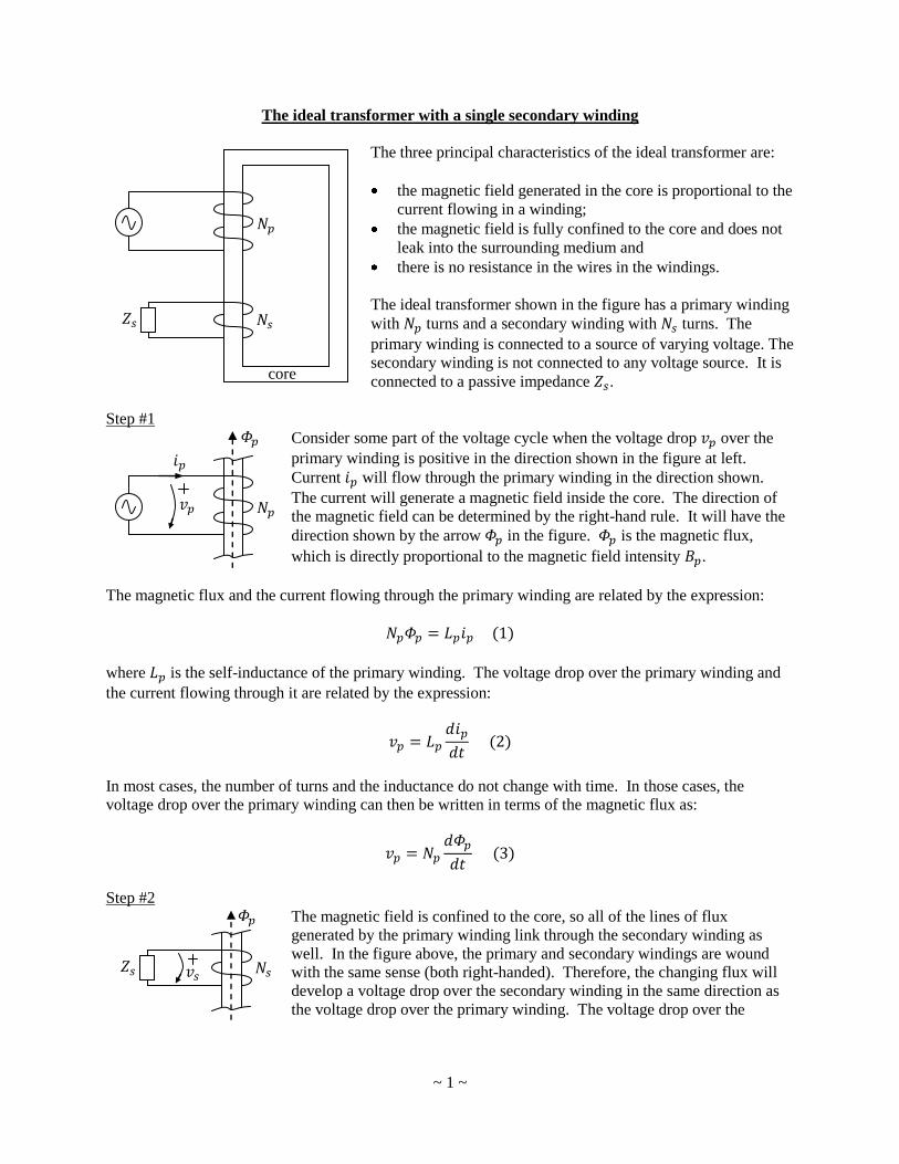
~ 1 ~

The ideal transformer with a single secondary winding

The three principal characteristics of the ideal transformer are:

the magnetic field generated in the core is proportional to the

current flowing in a winding;

the magnetic field is fully confined to the core and does not

leak into the surrounding medium and

there is no resistance in the wires in the windings.

The ideal transformer shown in the figure has a primary winding

with turns and a secondary winding with turns. The

primary winding is connected to a source of varying voltage. The

secondary winding is not connected to any voltage source. It is

connected to a passive impedance .

Step #1

Consider some part of the voltage cycle when the voltage drop over the

primary winding is positive in the direction shown in the figure at left.

Current will flow through the primary winding in the direction shown.

The current will generate a magnetic field inside the core. The direction of

the magnetic field can be determined by the right-hand rule. It will have the

direction shown by the arrow in the figure. is the magnetic flux,

which is directly proportional to the magnetic field intensity .

The magnetic flux and the current flowing through the primary winding are related by the expression:

where is the self-inductance of the primary winding. The voltage drop over the primary winding and

the current flowing through it are related by the expression:

In most cases, the number of turns and the inductance do not change with time. In those cases, the

voltage drop over the primary winding can then be written in terms of the magnetic flux as:

Step #2

The magnetic field is confined to the core, so all of the lines of flux

generated by the primary winding link through the secondary winding as

well. In the figure above, the primary and secondary windings are wound

with the same sense (both right-handed). Therefore, the changing flux will

develop a voltage drop over the secondary winding in the same direction as

the voltage drop over the primary winding. The voltage drop over the

core

~ 2 ~

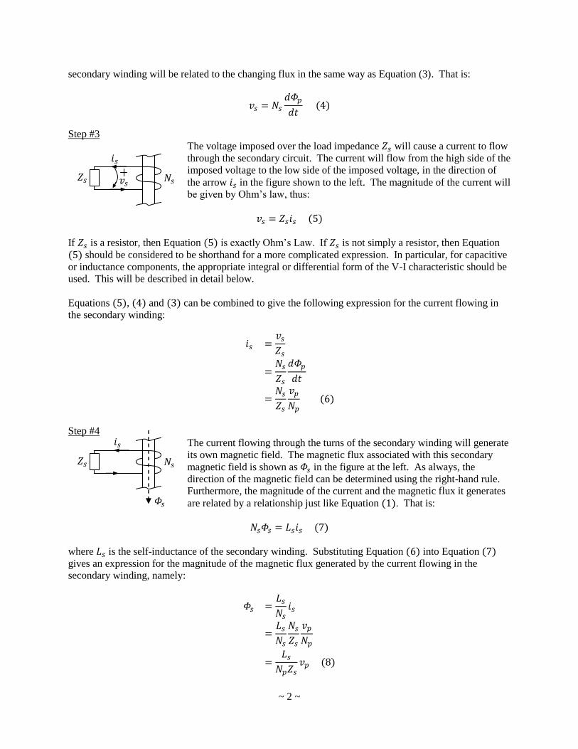
secondary winding will be related to the changing flux in the same way as Equation (3). That is:

Step #3

The voltage imposed over the load impedance will cause a current to flow

through the secondary circuit. The current will flow from the high side of the

imposed voltage to the low side of the imposed voltage, in the direction of

the arrow in the figure shown to the left. The magnitude of the current will

be given by Ohm’s law, thus:

If is a resistor, then Equation is exactly Ohm’s Law. If is not simply a resistor, then Equation

should be considered to be shorthand for a more complicated expression. In particular, for capacitive

or inductance components, the appropriate integral or differential form of the V-I characteristic should be

used. This will be described in detail below.

Equations , and can be combined to give the following expression for the current flowing in

the secondary winding:

Step #4

The current flowing through the turns of the secondary winding will generate

its own magnetic field. The magnetic flux associated with this secondary

magnetic field is shown as in the figure at the left. As always, the

direction of the magnetic field can be determined using the right-hand rule.

Furthermore, the magnitude of the current and the magnetic flux it generates

are related by a relationship just like Equation . That is:

where is the self-inductance of the secondary winding. Substituting Equation into Equation

gives an expression for the magnitude of the magnetic flux generated by the current flowing in the

secondary winding, namely:

~ 3 ~

Step #5

All of the lines of flux generated by the secondary winding circumnavigate

the core and link through the primary winding. The changing flux will

develop an additional voltage drop over the primary winding. The direction

of this voltage drop will be as shown in the figure to the left. (Compare with

Step #2.)

This voltage drop , which is induced in the primary winding due to

activity in the secondary winding, is a differential voltage. It can be thought

of as an addition to or subtraction from the voltage drop described in Step #1.

The additional voltage drop developed over the primary winding will be related to the changing flux in

the same way as Equation (3). That is:

Substituting Equation gives:

Step # 6

A differential current will flow in the primary winding in response to the

differential voltage . The power supply will deliver this current, as

needed, in just the amount which corresponds to the flux . The expression

in Equation , which governs the relationship between the primary current

and the primary flux , will govern this new relationship as well.

Note that the direction of the differential current is the same as the original primary current . Re-

arranging Equation and then substituting from Equation , gives:

Step #7

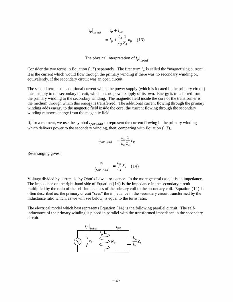
The total current flowing in the primary winding is the sum of the original primary current and

the additional, or differential, current induced in the primary winding by the activity in the secondary

circuit. We can write:

~ 4 ~

The physical interpretation of

Consider the two terms in Equation separately. The first term is called the “magnetizing current”.

It is the current which would flow through the primary winding if there was no secondary winding or,

equivalently, if the secondary circuit was an open circuit.

The second term is the additional current which the power supply (which is located in the primary circuit)

must supply to the secondary circuit, which has no power supply of its own. Energy is transferred from

the primary winding to the secondary winding. The magnetic field inside the core of the transformer is

the medium through which this energy is transferred. The additional current flowing through the primary

winding adds energy to the magnetic field inside the core; the current flowing through the secondary

winding removes energy from the magnetic field.

If, for a moment, we use the symbol to represent the current flowing in the primary winding

which delivers power to the secondary winding, then, comparing with Equation ,

Re-arranging gives:

Voltage divided by current is, by Ohm’s Law, a resistance. In the more general case, it is an impedance.

The impedance on the right-hand side of Equation is the impedance in the secondary circuit

multiplied by the ratio of the self-inductances of the primary coil to the secondary coil. Equation is

often described as: the primary circuit “sees” the impedance in the secondary circuit transformed by the

inductance ratio which, as we will see below, is equal to the turns ratio.

The electrical model which best represents Equation is the following parallel circuit. The self-

inductance of the primary winding is placed in parallel with the transformed impedance in the secondary

circuit.

~ 5 ~

The voltage-current characteristic of the transformer

Equation is not very handy for use in a mathematical circuit model. It involves two currents and the

total voltage drop over the primary winding. More convenient would be an expression involving only

one of the currents and the voltage drop. We can readily derive what we need. Let us take the first

derivative of Equation with respect to time.

We can substitute Equation to remove the reference to on the right-hand side. We get:

This is a differential equation, but it involves only the total voltage drop over the primary winding and

the total current flowing into the primary winding.

The relationship between the magnetic flux and the magnetic field intensity

The description above involved the magnetic flux . In general, “fluxes” are measures of some quantity

over, or passing through, or somehow related to, a two-dimensional area. The magnetic flux is a measure

of the number of magnetic field lines passing through a given area. More precisely, it is a measure of the

magnetic field intensity over an area perpendicular to the direction of the magnetic field.

In any three-dimensional region containing a magnetic field, it will always be possible to consider smaller

and smaller bits of area. In the limit, the bits of area can be made small enough that the magnetic field

intensity can be considered to be uniform in and around the bit of area. In one’s imagination, the bit of

area can then be re-oriented so that it is perpendicular to the direction of the magnetic field.

If is a small bit of area which is perpendicular to the magnetic field at the point of interest, then the flux

density and field intensity are related by scalar multiplication as:

In the more general case, when the given bit of area is not perpendicular to the lines of the magnetic field,

we would describe the area using a vector . The length of the vector would be set equal to the area

enclosed and the direction of the vector would be set perpendicular to the plane containing the enclosed

area. Using vectors and for the magnetic flux and magnetic field intensity, respectively, the

relationship would be written as a vector dot-product, thus:

If the ideal transformer (no leakage of magnetic field lines) has the same cross-section along its perimeter,

then the magnetic flux and magnetic field intensity will be the same at every cross-section, and their ratio

will be the same at every cross-section.

~ 6 ~

The ratio of self-inductances and the turns ratio

Two windings on a transformer are often compared using the ratio of their number of turns. Equation

applies to both of the windings, that is:

Let us make two explicit assumptions: (i) that the number of turns is a constant with time (it may not be a

constant if the inductor is a variable inductor) and (ii) that the windings have constant configurations

(they may not if the stresses in the wires cause the windings to deform). If the windings’ inductances and

numbers of turns are constant, then these equations can be re-written as follows, with the constants on the

right-hand side.

Now, let us make two additional explicit assumptions: (iii) that the core material is the same underneath

both windings and (iv) that the cross-sections of the core are the same within both windings. Then, the

currents which generate equal flux are:

We know that the currents in the two windings are related by the turns ratio in the following way:

Substituting gives:

Which can be re-arranged as:

The magnetic field intensity inside the core

For a circular loop of thin wire in a flat plane, the instantaneous magnetic field intensity at the center of

the loop is given by:

~ 7 ~

where

N/m2 is the permeability of free space;

is a dimensionless quantity which is the ratio of the permeability of the core material to the

permeability of free space;

is the instantaneous current flowing through the loop and

is the radius of the loop.

The magnetic field at the center of the loop is perpendicular to the plane of the loop

and oriented in the direction determined by the right-hand rule. The magnetic field is measured in Tesla.

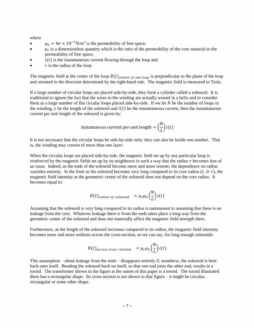
If a large number of circular loops are placed side-by-side, they form a cylinder called a solenoid. It is

traditional to ignore the fact that the wires in the winding are actually wound in a helix and to consider

them as a large number of flat circular loops placed side-by-side. If we let be the number of loops in

the winding, be the length of the solenoid and be the instantaneous current, then the instantaneous

current per unit length of the solenoid is given by:

It is not necessary that the circular loops be side-by-side only; they can also be inside one another. That

is, the winding may consist of more than one layer.

When the circular loops are placed side-by-side, the magnetic field set up by any particular loop is

reinforced by the magnetic fields set up by its neighbours in such a way that the radius becomes less of

an issue. Indeed, as the ends of the solenoid become more and more remote, the dependence on radius

vanishes entirely. In the limit as the solenoid becomes very long compared to its core radius ( ), the

magnetic field intensity at the geometric center of the solenoid does not depend on the core radius. It

becomes equal to:

Assuming that the solenoid is very long compared to its radius is tantamount to assuming that there is no

leakage from the core. Whatever leakage there is from the ends takes place a long way from the

geometric center of the solenoid and does not materially affect the magnetic field strength there.

Furthermore, as the length of the solenoid increases compared to its radius, the magnetic field intensity

becomes more and more uniform across the cross-section, so we can say, for long enough solenoids:

This assumption – about leakage from the ends – disappears entirely if, somehow, the solenoid is bent

back onto itself. Bending the solenoid back on itself, so that one end joins the other end, results in a

toroid. The transformer shown in the figure at the outset of this paper is a toroid. The toroid illustrated

there has a rectangular shape. Its cross-section is not shown in that figure – it might be circular,

rectangular or some other shape.

~ 8 ~

In any event, when the winding is bent back on itself to form a toroid, the assumption that the core is

“long” compared its radius is automatically satisfied. Even so, the assumption that there is no leakage –

through the surface, for example – is still necessary for the equations above to apply.

Toroids often have a circular perimeter (this is not a statement about the cross section). The following

figure shows the dimensions of a toroid with a circular perimeter. Once again, the cross-section is not

shown in the figure.

The core will have a physical outer radius and a physical inner radius. In addition, it will have an

effective radius, which may depend, among other factors, on the shape of the cross-section. The effective

circumference of the toroidal core will be . Then, inside the toroid, the

magnetic field intensity will be given by:

In most cases, the manufacturer will specify the effective length of the toroid, using the parameter . In

that case, the magnetic field intensity will be given by:

In the ideal case, the magnetic field intensity will be a constant across the entire cross-section of the

toroid. Even if the field is not uniform across the entire cross-section, the expression in Equation

still applies. In that case, it is the maximum value of the field intensity.

The maximum value of the field intensity is important to know. If the applied current becomes too high,

the magnetic field inside the toroid will increase to a strength beyond the material’s ability to handle. In

general, the material from which the core is made contains a number of small regions called “domains”.

In response to an externally applied magnetic field, the domains will re-orient themselves in the direction

of the applied field. As the external field strength increases, more domains will re-orient themselves and

the re-oriented domains will become more closely aligned to the direction of the applied field. But, there

is a limit to how far the material can respond. At some point, called “saturation”, the material will have

done all of the re-orienting it can. Further increases in the strength of the external field will have no

effect.

It is important to ensure that the current flowing through the winding(s) in a toroidal transformer do not

drive the core too close to its saturation point, or energy will be wasted. In general, a circuit should be

designed so that the magnetization of the core never exceeds 70% or so of the saturation value.

~ 9 ~

Loads in the secondary circuit which are not resistors

In the discussion above, the symbol was used for the load in the secondary circuit. The equations were

written as if this impedance was a resistor. More is needed if the impedance has capacitive and/or

inductive characteristics. In the most general case, the load will have a resistance component , a

capacitive component and an inductive component . The subscript “sec” is used for these

secondary circuit impedances to ensure that there is never any confusion between and . The

former is the self-inductance of the secondary winding; the latter is the inductive component of the load.

For illustrative purposes, let us assume that the impedance components are in series, as shown in the

following figure.

The voltage drops over the three components are , and , respectively. At all times, the sum

of these three voltage drops must equal the voltage drop over the secondary winding. Since all the

components are in series, the same current flows through them all. The voltage-current characteristics

of the three components are as follows:

The sign of the second V-I characteristic is positive because a positive current (as shown in the figure)

adds charge to the capacitor and thereby increases its voltage. The sign of the third V-I characteristic is

also positive because an increasing current increases the EMF over the inductor which opposes the

driving voltage . The capacitor’s integral is assumed to start at time when the voltage over the

capacitor is equal to .

The differential equation which governs the secondary circuit is therefore as follows:

Equation is the more general form of Equation . In the case where the impedance in the

secondary circuit is entirely resistive, Equation reduces to Equation . We can work our way

through the equations following Equation using this more general form.

Equation would be written as:

~ 10 ~

Equation remains unchanged and Equation would be written as:

Equation remains unchanged, but is more useful to us if we express it in integral form as:

in which case Equation would be written as:

Equation remains unchanged, but is more useful to us if re-arranged to give:

and Equation would be written as:

Equations and are a pair of equations which relate the magnetizing voltage drop over the

primary winding to the differential voltage drop over the primary winding and the differential current

flowing through the primary winding.

Equation can be re-written as:

Now, Equation also remains unchanged. It states that the total current flowing in the primary circuit

is the sum of the magnetizing current and the differential current due to activity in the secondary

circuit. It is more useful to us if re-arranged to be:

~ 11 ~

in which case Equation becomes:

Let us define an “impedance operator” by the following definition. The impedance operator

“operates” on a current to give a voltage. We could write the impedance operator as if it was a function

of the current, in a form like . (In fact, this is exactly what the impedance operator is – a function of

the current.)

Using the impedance operator, Equations and can be written as:

These equations can be re-arranged as follows:

Equations and are the more general forms of Equations and , respectively, for a non-

resistive secondary load. There are only two differences: (i) a constant offset due to the initial charge on

the secondary capacitor and (ii) it is not possible to divide Equation through by the impedance

because it is an operator. Other than these, the two equations are the same as for the resistive case and the

interpretation is the same.

The inductance of windings on a toroid with a circular cross-section

Although it is not essential to a discussion about an ideal transformer, this is a handy place to describe the

formula for calculating the self-inductances of the windings on a toroidal core with a circular cross-

section. In Equation above, we calculated the magnetic field intensity inside the core of a toroid.

That expression is repeated here for convenience.

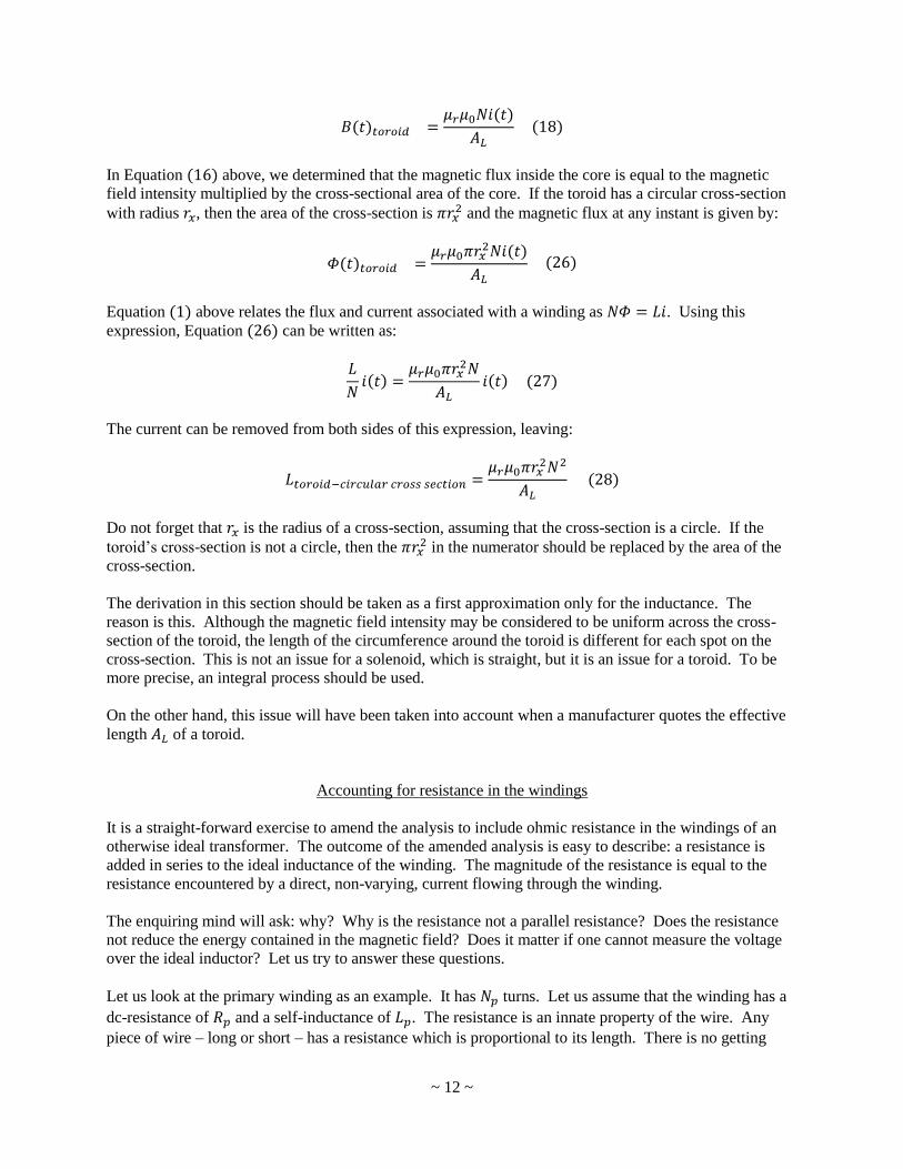
~ 12 ~

In Equation above, we determined that the magnetic flux inside the core is equal to the magnetic

field intensity multiplied by the cross-sectional area of the core. If the toroid has a circular cross-section

with radius , then the area of the cross-section is and the magnetic flux at any instant is given by:

Equation above relates the flux and current associated with a winding as . Using this

expression, Equation can be written as:

The current can be removed from both sides of this expression, leaving:

Do not forget that is the radius of a cross-section, assuming that the cross-section is a circle. If the

toroid’s cross-section is not a circle, then the in the numerator should be replaced by the area of the

cross-section.

The derivation in this section should be taken as a first approximation only for the inductance. The

reason is this. Although the magnetic field intensity may be considered to be uniform across the cross-

section of the toroid, the length of the circumference around the toroid is different for each spot on the

cross-section. This is not an issue for a solenoid, which is straight, but it is an issue for a toroid. To be

more precise, an integral process should be used.

On the other hand, this issue will have been taken into account when a manufacturer quotes the effective

length of a toroid.

Accounting for resistance in the windings

It is a straight-forward exercise to amend the analysis to include ohmic resistance in the windings of an

otherwise ideal transformer. The outcome of the amended analysis is easy to describe: a resistance is

added in series to the ideal inductance of the winding. The magnitude of the resistance is equal to the

resistance encountered by a direct, non-varying, current flowing through the winding.

The enquiring mind will ask: why? Why is the resistance not a parallel resistance? Does the resistance

not reduce the energy contained in the magnetic field? Does it matter if one cannot measure the voltage

over the ideal inductor? Let us try to answer these questions.

Let us look at the primary winding as an example. It has turns. Let us assume that the winding has a

dc-resistance of and a self-inductance of . The resistance is an innate property of the wire. Any

piece of wire – long or short – has a resistance which is proportional to its length. There is no getting

~ 13 ~

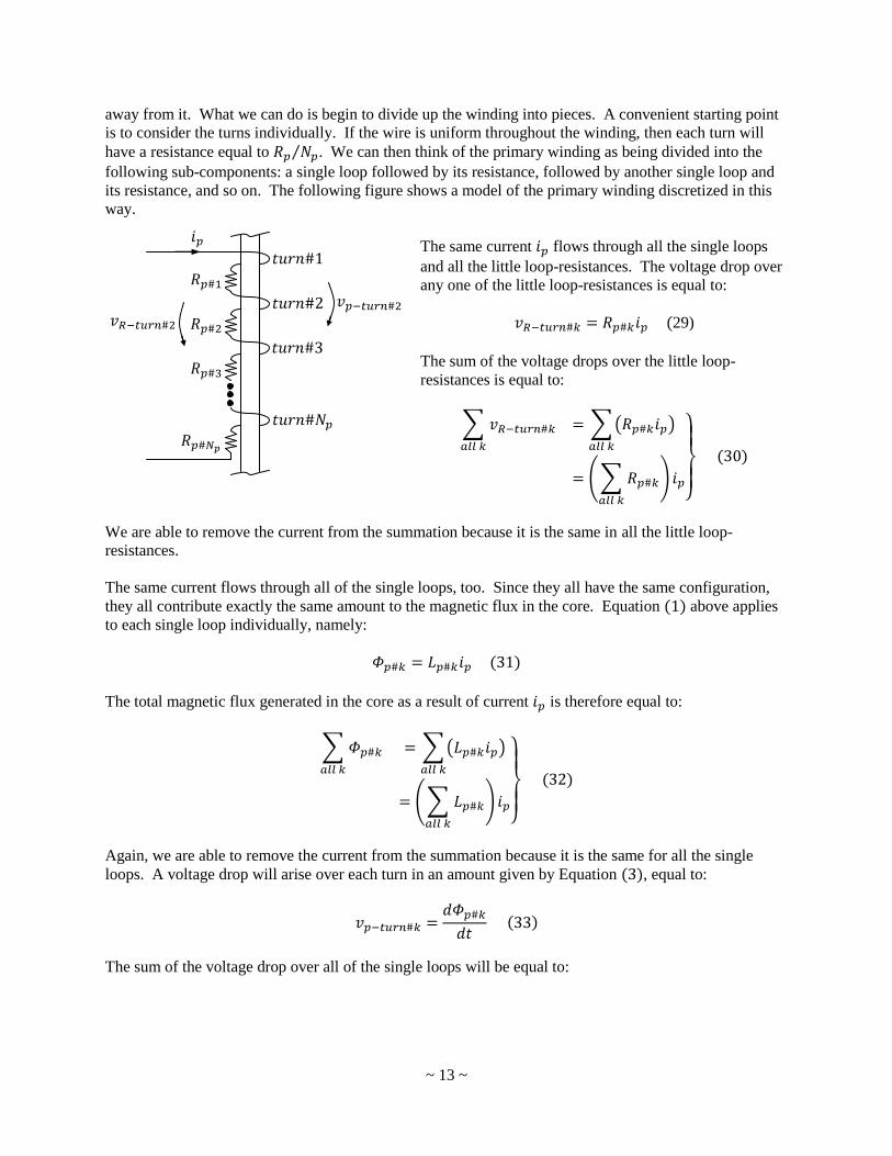
away from it. What we can do is begin to divide up the winding into pieces. A convenient starting point

is to consider the turns individually. If the wire is uniform throughout the winding, then each turn will

have a resistance equal to . We can then think of the primary winding as being divided into the

following sub-components: a single loop followed by its resistance, followed by another single loop and

its resistance, and so on. The following figure shows a model of the primary winding discretized in this

way.

The same current flows through all the single loops

and all the little loop-resistances. The voltage drop over

any one of the little loop-resistances is equal to:

29)

The sum of the voltage drops over the little loop-

resistances is equal to:

We are able to remove the current from the summation because it is the same in all the little loop-

resistances.

The same current flows through all of the single loops, too. Since they all have the same configuration,

they all contribute exactly the same amount to the magnetic flux in the core. Equation above applies

to each single loop individually, namely:

The total magnetic flux generated in the core as a result of current is therefore equal to:

Again, we are able to remove the current from the summation because it is the same for all the single

loops. A voltage drop will arise over each turn in an amount given by Equation , equal to:

The sum of the voltage drop over all of the single loops will be equal to:

~ 14 ~

Then, Equation can be used to say that:

Now, combining Equations and , we can say that the total voltage drop over the winding is

equal to:

Since the individual resistances of all the loop-resistances are the same and the individual inductances of

all the individual single loops are the same, then:

Resistors in series add up linearly, so that:

Inductors in series also add up linearly, so that:

where and are the total resistance and inductance of the winding, respectively. Then, Equation

becomes:

This is the circuit equation for a series combination of resistance and ideal self-inductance . All of

the magnetic effects arise from the second term in Equation and from the second term only. We can

continue to use the symbol to represent the second term and use it in the same way as it was used in all

of the preceding sections.

~ 15 ~

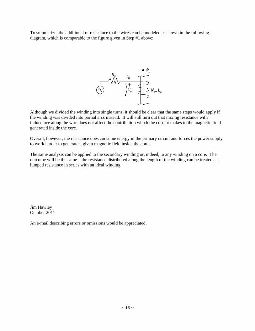
To summarize, the additional of resistance to the wires can be modeled as shown in the following

diagram, which is comparable to the figure given in Step #1 above:

Although we divided the winding into single turns, it should be clear that the same steps would apply if

the winding was divided into partial arcs instead. It will still turn out that mixing resistance with

inductance along the wire does not affect the contribution which the current makes to the magnetic field

generated inside the core.

Overall, however, the resistance does consume energy in the primary circuit and forces the power supply

to work harder to generate a given magnetic field inside the core.

The same analysis can be applied to the secondary winding or, indeed, to any winding on a core. The

outcome will be the same – the resistance distributed along the length of the winding can be treated as a

lumped resistance in series with an ideal winding.

Jim Hawley

October 2011

An e-mail describing errors or omissions would be appreciated.