the study of probability model for compound similarity searching
109
Final Project Report UTM Research Management Centre Project Vote – 75207 THE STUDY OF PROBABILITY MODEL FOR COMPOUND SIMILARITY SEARCHING PROJECT LEADER – ASSOC. PROF. DR. NAOMIE SALIM FACULTY OF COMPUTER SCIENCE AND INFORMATION SYSTEMS UNIVERSITY TECHNOLOGI MALAYSIA
Transcript of the study of probability model for compound similarity searching

Final Project Report
UTM Research Management Centre Project Vote – 75207
THE STUDY OF PROBABILITY MODEL
FOR
COMPOUND SIMILARITY SEARCHING
PROJECT LEADER – ASSOC. PROF. DR. NAOMIE SALIM
FACULTY OF COMPUTER SCIENCE AND INFORMATION SYSTEMS
UNIVERSITY TECHNOLOGI MALAYSIA
i
ABSTRACT
Information Retrieval or IR system main task is to retrieve relevant
documents according to the user’s query. One of IR most popular retrieval model is
the Vector Space Model. This model assumes relevance based on similarity, which
is defined as the distance between query and document in the concept space. All
currently existing chemical compound database systems have adapt the vector space
model to calculate the similarity of a database entry to a query compound. However,
it assumes that fragments represented by the bits are independent of one another,
which is not necessarily true. Hence, the possibility of applying another IR model is
explored, which is the Probabilistic Model, for chemical compound searching. This
model estimates the probabilities of a chemical structure to have the same bioactivity
as a target compound. It is envisioned that by ranking chemical structures in
decreasing order of their probability of relevance to the query structure, the
effectiveness of a molecular similarity searching system can be increased. Both
fragment dependencies and independencies assumption are taken into consideration
in achieving improvement towards compound similarity searching system. After
conducting a series of simulated similarity searching, it is concluded that PM
approaches really did perform better than the existing similarity searching. It gave
better result in all evaluation criteria to confirm this statement. In terms of which
probability model performs better, the BD model shown improvement over the BIR
model.

ii
ABSTRAK
Tujuan utama sistem pencarian maklumat atau IR (Information Retrieval)
adalah untuk mencari dokumen yang relevan berdasarkan permintaan pengguna.
Salah sebuah model IR yang popular adalah model ruang-vektor. Model in
menganggap bahawa sesebuah dokumen itu adalah relevan kepada sesuatu
pertanyaan berdasarkan keserupaan antara keduanya. Ia ditakrif sebagai jarak di
antara dokumen dan permintaan pengguna (atau query), dalam sebuah ruang konsep.
Model ruang-vektor ini telah diaplikasikan ke dalam sistem pencarian sebatian kimia
yang serupa. Walau bagaimanapun, ia menganggap bit-bit yang mewakili pecahan-
pecahan molekul kimia sebagai saling tidak berkait antara satu sama lain. Ini adalah
tidak semestinya benar dalam keadaan sebenar. Maka, projek ini mencadangkan
perlaksanaan pencarian keserupaan alternatif, iaitu dengan mengaplikasikan sebuah
lagi model IR iaitu model kebarangkalian. Model ini akan menganggarkan
kebarangkalian samada sesebuah struktur kimia itu mempunyai bioaktiviti yang
serupa dengan molekul pertanyaan ataupun tidak. Ini dijangka dapat menghasilkan
sebuah sistem yang mempunyai keberkesanan yang lebih baik untuk pengguna. Ini
adalah kerana struktur dinilai dan dipaparkan mengikut susunan menurun
kebarangkalian sesebuah struktur itu aktif, terhadap pertanyaan pengguna. Kedua-
dua anggapan kebersandaran dan ketidaksandaran bit pada struktur kimia, akan
dipertimbangkan untuk menghasilkan sistem pencarian keserupaan yang berkesan.
Hasil eksperimen menyimpulkan bahawa pencarian keserupaan berdasarkan model
kebarangkalian adalah lebih berkesan daripada pencarian keserupaan yang sedia ada.
Selain daripada itu, adalah didapati bahawa model kebarangkalian berdasarkan
anggapan kebersandaran bit menghasilkan keputusan yang lebih baik berbanding
dengan anggapan ketidaksandaran bit.

iii
TABLE OF CONTENT
CHAPTER TITLE PAGE
ABSTRACT
ABSTRAK
TABLE OF CONTENT
i
ii
iii
1
INTRODUCTION
1.1 Background of Problem
1.2 Problem Statement
1.3 Project Objectives
1.4 Scope
1.5 Expected Contribution
1.6 Organisation of Report
1.7 Summary
1
1
3
3
4
5
6
7
2 LITERATURE REVIEW 2.1 Searching Methods for Databases of Molecules
2.1.1 Structure Searching
2.1.2 Substructure Searching
2.1.3 Similarity Searching
2.1.4 Post-searching Processing of Results
8
9
9
11
13
15

iv
2.2 Representation of Chemical Structures
2.2.1 1D Descriptors
2.2.2 2D Descriptors
2.2.3 3D Descriptors
2.3 Similarity Coefficients
2.4 Information Retrieval
2.4.1 Retrieval Process
2.4.2 Classical Retrieval Model
2.5 Vector Space Model (VSM)
2.6 Probability Model (PM)
2.6.1 Binary Independence Retrieval (BIR) Model
2.6.1.1 Retrieval Status Value (RSV)
2.6.1.2 Probability Estimation and
Improvement
2.6.2 Binary Dependence (BD) Model
2.6.2.1 Dependence Tree
2.6.2.2 Retrieval Status Value (RSV)
2.6.2.3 Probability Estimation and
Improvement
2.7 Discussion
2.8 Summary
16
16
17
20
20
25
26
27
29
33
36
37
39
42
44
46
48
50
52
3
METHODOLOGY
3.1 Computational Experiment Design
3.2 Test Data Sets
3.3 Structural Descriptors
54
54
55
56

v
3.4 Experiment 1: Comparing the Effectiveness of
Similarity Searching Method
3.4.1 Vector Space Model
3.4.2 Binary Independence Retrieval Model
3.4.3 Binary Dependence Model
3.4.4 Performance Evaluation
3.5 Experiment 2: Comparing the Query Fusion
Result of Similarity Searching Method
3.5.1 Binary Independence Retrieval Model
3.5.2 Binary Dependence Model
3.5.3 Performance Evaluation
3.6 Hardware and Software Requirements
3.7 Discussion
3.8 Summary
58
58
59
63
69
71
74
74
76
76
77
79
4 RESULTS AND DISCUSSIONS
4.1 Result of VSM-based Similarity Searching
4.2 Result of BIR-based Similarity Searching
4.3 Result of BD-based Similarity Searching
4.4 Discussion
4.5 Summary
80
82
83
83
84
90
5
CONCLUSION
5.1 Summary of Work
5.2 Future Work
91
91
92
REFERENCES
94

vii
TABLE OF CONTENT
CHAPTER TITLE PAGE
TITLE PAGE
ABSTRACT
ABSTRAK
TABLE OF CONTENT
i
ii
iii
iv
1
INTRODUCTION
1.1 Background of Problem
1.2 Problem Statement
1.3 Project Objectives
1.4 Scope
1.5 Expected Contribution
1.6 Organisation of Report
1.7 Summary
1
1
3
3
4
5
6
7
2 LITERATURE REVIEW
2.1 Searching Methods for Databases of Molecules
2.1.1 Structure Searching
2.1.2 Substructure Searching
2.1.3 Similarity Searching
2.1.4 Post-searching Processing of Results
8
9
9
11
13
15

viii
2.2 Representation of Chemical Structures
2.2.1 1D Descriptors
2.2.2 2D Descriptors
2.2.3 3D Descriptors
2.3 Similarity Coefficients
2.4 Information Retrieval
2.4.1 Retrieval Process
2.4.2 Classical Retrieval Model
2.5 Vector Space Model (VSM)
2.6 Probability Model (PM)
2.6.1 Binary Independence Retrieval (BIR)
Model
2.6.1.1 Retrieval Status Value (RSV)
2.6.1.2 Probability Estimation and
Improvement
2.6.2 Binary Dependence (BD) Model
2.6.2.1 Dependence Tree
2.6.2.2 Retrieval Status Value (RSV)
2.6.2.3 Probability Estimation and
Improvement
2.7 Discussion
2.8 Summary
16
16
17
20
20
25
26
27
29
33
36
37
39
42
44
46
48
50
52
3
METHODOLOGY
3.1 Computational Experiment Design
3.2 Test Data Sets
3.3 Structural Descriptors
3.4 Experiment 1: Comparing the Effectiveness of
Similarity Searching Method
3.4.1 Vector Space Model
54
54
55
56
58
58
ix
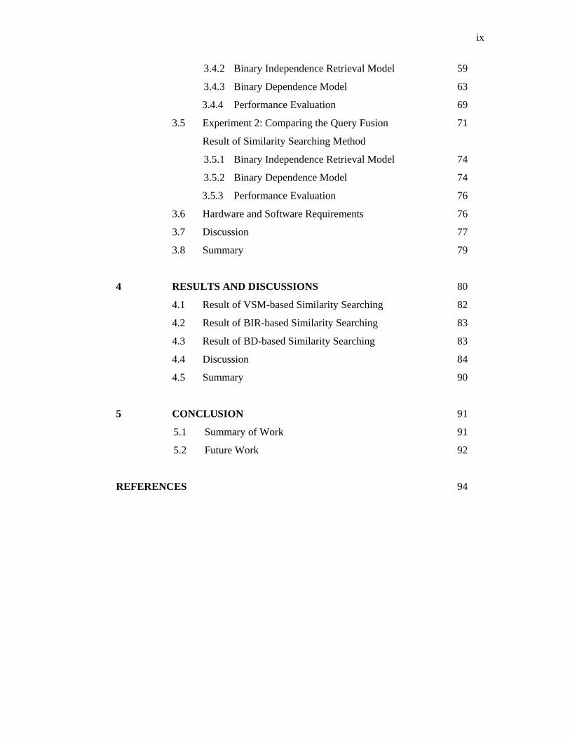
3.4.2 Binary Independence Retrieval Model
3.4.3 Binary Dependence Model
3.4.4 Performance Evaluation
3.5 Experiment 2: Comparing the Query Fusion
Result of Similarity Searching Method
3.5.1 Binary Independence Retrieval Model
3.5.2 Binary Dependence Model
3.5.3 Performance Evaluation
3.6 Hardware and Software Requirements
3.7 Discussion
3.8 Summary
59
63
69
71
74
74
76
76
77
79
4 RESULTS AND DISCUSSIONS
4.1 Result of VSM-based Similarity Searching
4.2 Result of BIR-based Similarity Searching
4.3 Result of BD-based Similarity Searching
4.4 Discussion
4.5 Summary
80
82
83
83
84
90
5
CONCLUSION
5.1 Summary of Work
5.2 Future Work
91
91
92
REFERENCES
94

CHAPTER 1
INTRODUCTION
1.1 Background of Problem
Cheminformatics is now being extensively used by the pharmaceutical and
agrochemical companies, to find new active compounds and bring them to market as
quickly as possible. Highly sophisticated systems have been developed for the
storage, retrieval and processing of a range of types of chemical information.
Although chemical structures differ greatly from other entities that are commonly
stored in database, some parallels can be drawn between chemical database searches
and searches on words or documents (Miller, 2002). Hence, this project focuses on
two different fields: the chemical retrieval system as well as the information retrieval
system. Here, an alternative chemical search method is proposed based on the
concepts obtained from the information retrieval model.
Information retrieval (IR) is a science or art of locating and obtaining
documents based on information needs expressed to a system in a query language.
Hence, IR systems need to interpret the content of documents or information items in
a collection and rank them according to their degree of relevance. IR systems have

2
expanded rapidly due to the vast usage of Internet. Many new approaches have been
introduced to facilitate user’s task in finding information to be used in problem
solving and achieving their goals. Previous methods, like the Boolean Model are no
longer sufficient in retrieving relevant documents, mainly because it pays little
attention to the ranking of the result retrieved and has limited features in query
formulation and processing (Croft, 1995). As a result, IR research turns to partial
match methods, which consist of two retrieval models: the Vector Space Model
(Salton and Buckley, 1988a) and the Probability Model (van Rijsbergen, 1979; Fuhr,
1992). Vector space assumes that relevance is based on similarity measures that are
defined as the distance between query and document in the concept space. It
represents documents and query by vectors in the space whose elements are their
values on the different dimensions. Similarity measure measures the cosines angle
between document- vector and query-vector. Probability model on the other hand,
estimates the probabilities of relevance or non-relevance of a document to an
information need.
Chemical compound databases have now been widely used to assist in the
development of new drugs. It has progressed from being a mere repository of
compound synthesized within an organisation, to being a powerful research tool for
discovering new lead compounds, worthy of further synthetic or biological study.
One of the facilities provided for this purpose is the similarity searching tool, in
which the database can be searched for compounds similar to a query compound.
The main use for this tool is to find other compounds similar to a potential drug
compound, with the hope that these similar compounds have similar activity to the
query compound and can be better optimised as drugs compared to the initial
compound.
Thus, there is always a need to develop new similarity searching methods.
This project is an example of an effort to develop a new similarity searching method
to help researchers find lead compounds faster and more effectively.

3
1.2 Problem Statement
Due to the similarities in the way that chemical and textual database records
are characterised, many algorithms developed for the processing of textual databases
are also applicable to the processing of chemical structure database and vice versa
(Willett, 2000). For instance, all existing chemical compound similarity searching
systems applies the Vector Space Model (VSM). Even though this approach has
acceptable retrieval effectiveness (Salim, 2002), the VSM only considers structural
similarity, ignoring both activity and inactivity. Other than that, the evaluation order
of the query and the database compounds was not taken into account. It also
assumes that fragments are independent of all other fragments, which is not
necessarily true (Yates and Neto, 1999).
Hence, this project focuses on developing a similarity searching method
based on the Probability Model (PM). It is a stronger theoretical model and there are
many approaches in this model (Crestani, et al., 1998). However, only two
approaches are used here that are the Binary Independence Retrieval (BIR) Model
and Binary Dependence (BD) Model. Their implementation and effectiveness in
performing similarity searching has never been experimented or compared with the
present similarity searching method.
1.3 Project Objectives
The following are objectives for this project:
a) To develop a new compound similarity searching method which is based
on the PM as stated as below:

4
BIR model, which is the most simple model and basic of all
approaches in PM, assuming linked dependence.
BD model, which is a more realistic approach in retrieving active
structures, where presence or absence of a bit gives effect to the
presence or absence of another.
b) To test the effectiveness of each similarity searching method developed
based on its ability to give similar active compounds to the target
compound.
1.4 Scope
The scope of this project is as follows:
a) Probability-based compound similarity searching is based on the BIR and
BD model.
b) Vector space-based compound similarity searching uses the Tanimoto
coefficient to calculate the similarity measure.
c) All representation of the chemical compound is in the form of binary
descriptor. The Barnard Chemical Information (BCI) bit-string is used
which is a dictionary-based bit sting.
d) Testing is done on the National Cancer Institute (NCI) AIDS dataset.
1.5 Significance of Study
Many research works have been done on vector space based similarity
searching. As mention earlier, it is not without its limitations. Thus, the focus of this
5
project is to take up other alternatives of IR and apply it in compound similarity
searching. PM takes into account both activity and inactivity of a chemical
compound, unlike VSM, which only considers structural similarity. Hence, research
work should be done to develop a similarity searching based on PM, and compare its
effectiveness with the current similarity searching methods.
Currently, there are many similarity searching methods developed and much
effort is given in improving them. The question now, is why the need of another
similarity searching method? Bajorath (2002) refers to virtual screening of
compounds as an “algorithm jungle”. However, the fact is biological activity is more
diverse and complicated than can be addressed by a single method. Different
methods rank active compounds differently and thus selecting different subsets of
actives. This can lead to the fact that a method can find some actives that all other
methods would miss.
Sheridan and Kearsley (2002) mentioned that looking for the best way in
searching chemical database can be a pointless exercise. However, the authors also
mentioned that multiple methods are still needed, as stated below:
It is as if we have a set of imperfect windows through which to view
Nature. As computational scientists, we get nearer to the truth by
looking through as many different windows as possible.
(Sheridan and Kearsley, 2002: 910)
6
1.6 Organisation of Report
The outline for this research report is as follows:
Chapter 2 covers the literature review of this project, which is divided into 2
parts. The first part discusses about the current similarity searching method. This
section will also describe the requirements of similarity searching. Firstly molecular
descriptors are discussed. Similarity values obtained depends heavily on the set of
descriptors used. Descriptors are vectors of numbers, each of which is based on a
predefined attribute. It can be classified into 1D, 2D and 3D. Next, similarity
coefficient is discussed. Similarity coefficients are used to obtain a numeric
quantification to the degree of similarity between a pair of structures. Basically there
are four main types of similarity coefficients that will be discussed, which are
distance, association, correlation and probabilistic. The second part explains about
the models in IR in terms of the definition and mathematical structures. Both the
VSM and PM are discussed. The PM mainly focuses on the BIR and BD model.
Discussion is also done in this chapter, to relate both the chemical database and IR
domain.
Chapter 3 discuses the methodology used in this project. It covers
experimental design as well as performance evaluation. Results of the experiments
conducted are recorded in Chapter 4. There is also a discussion which includes
critical analysis and result comparison of the performance evaluation done. Finally,
Chapter 5 concludes this report.

7
1.7 Summary
There is always a need to develop new similarity searching methods to find
lead compounds more effectively and thus reduce the time needed to develop new
drugs. Since, there are resemblances between conducting chemical database searches
and searches on documents; hence, this project proposes an alternative chemical
search method based on the concepts obtained from the IR domain (i.e. the BIR and
BD model). We have discussed in this chapter the objectives, scope and significance
of this project, to set the context for the work explained further in the research report.

CHAPTER 2
LITERATURE REVIEW
This chapter is divided into two parts. The first part covers topics on the
current chemical database search method emphasizing on how similarity searching
complements the early search methods like structure searching and substructure
searching. Performance of similarity searching is very much influenced by the
similarity coefficient used to measure the likeness between structures. This in turn,
depends on how chemical structures are represented. Hence these two requirements
are also covered in this chapter.
The second part of this chapter discusses about the models in information
retrieval (IR). Both the VSM and PM are discussed. This project focuses on
Probability Model. There are many approaches in this model as mentioned by
Crestani, et al. (1998). However, only two approaches are used here. The first is the
Binary Independence Retrieval (BIR) Model, which is a simple model assuming
independence of terms. The second approach in probability model is Binary
Dependence (BD) Model, which is the opposite of the independence assumptions. It
however yields a more realistic approach in retrieving relevant documents.

9
Discussion is also done in this chapter, to relate both the chemical database
and IR domain. Here, the similarity between current compound search method and
Vector Space Models is shown. Algorithms developed for the processing of textual
databases are also applicable to the processing of chemical structure database
(Willett, 2000). This has been the basis of this project. Another alternative in
compound similarity searching is proposed that is based on Probability Model. Apart
from having a strong theoretical basis, PM is a more realistic approach in retrieval
system. It will rank chemical compounds in decreasing order of their probability of
being similarly active to the target compound. According to the Probability Ranking
Principle (PRP), if the ranking of the compounds is in decreasing probability of
usefulness to the user, then the overall effectiveness of the system to its users will be
the best (Cooper, 1994).
2.1 Searching Methods for Databases of Molecules
There are three different retrieval mechanisms offered by the chemical
databases. There are the structure searching, substructure searching and similarity
searching. Structure searching and substructure searching are used by the early
chemical information systems. There were later complemented by similarity
searching, which is the focus of this project.
2.1.1 Structure Searching
Structure searching involves searching for a molecule of database for a
specified query molecule. It is also known as the exact-match searching (Miller,
2002). This searching mechanism is done by firstly asking the user to supply the

10
complete structure of a molecule. At this moment, user must already have a well
defined specification on their mind. The database is then searched for compound
that matches perfectly with the target structure. Comparison to determine
equivalence is done using the graph isomorphism algorithm, where chemical
structure is treated as graph. A graph is generated for each compound based on its
connection table. Atoms in the chemical structure are denoted as vertices whereas
their bonds are denoted by their edges. Searching is done by checking the graph
describing the query molecule with the graphs of each of the database molecules for
isomorphism. Two graphs are isomorphic if there is 1:1 corresponding between
vertices and 1:1 corresponding between edges, with corresponding edges joining
corresponding vertices.
Structure searching is performed to find out whether a proposed new structure
already exists in a database. This is to ensure that the structure is novel and never
been identified before. If it is not in the database, then the new structure is registered
in a structure file, also known as a register file, in which there is only a single and
unique record of each compound. Some additional information about the new
structure can also be recorded in an associated data file. Hence, a structure searching
can also be used to get some additional data about a particular compound.
A structure search might yield no hits even though the compound is present in
the database. This is depending on the flexibility of the query specification. Other
than that, this type of search is also very time consuming. This due to the number of
different connection tables that can be constructed for a compound, that is N! for N-
atom molecule (Salim, 2002).

11
Table 2.1: Overview of structure searching
Structure searching
Question: Which molecule in a database matches exactly with the
specified structure?
Query requires: An entire specification of a molecule.
Application:
Identify whether compound exist in database or not.
To get some data about a particular compound e.g.
associated biological test results.
Limitation:
Time consuming.
User must already have a well-defined specification to
avoid no-hits even though structure is in the database.
2.1.2 Substructure Searching
Substructure searching involves the user specifying a set of pieces of a
chemical structure and requests the system to return a set of compounds that contain
the pieces. This is done by undergoing detailed atom-by-atom graph matching in
which each and every atom and bond in the query substructure is mapped onto the
atoms and bonds of each database structure. This is to determine whether subgraph
isomorphism is present. However, checking of subgraph isomorphism has an NP-
complete nature (Gillet et al., 1998), which means that it is totally infeasible to be
implemented especially on large databases. This is why, substructure searching has
become a two stage procedure, where the first stage involves pre-screening of the
database to eliminate structures that cannot possibly match the query. The remaining
structure will then undergo the final, time-consuming atom-by-atom search.
Pre-screening of structures can be done by using structural keys. Keys
encode the presence or absence of specific structural features. Detailed explanation
12
is given in the next section. Basically, keys are generated when the structures are
registered in the database. A key is created by defining the structural features of
interest, assigning a bit (1 represents presence, 0 represents absence) to each one of
these features and generating a bitmap for each compound in the database. At search
time, only those structures that have all the keys set by the query structure need to be
examined for atom-by-atom mapping.
The purpose of this search mechanism is to find structures containing a
specified functional group, thus allowing the properties common to that group to be
observed. It can also be used in the implementation of pharmacophoric pattern
searching, where compounds containing a specific 3D substructure that has been
identified in a molecular modelling study, are sought.
Although substructure searching provides invaluable tool for accessing
databases of chemical structures, it does pose several limitations. First, the user
posing the query must already have acquired a well defined view of what sorts of
structures are expected to be retrieved from the database. They can also tell while
browsing the hits, how each answer satisfied the search question. Second, there is
very little control on the size of the output produced. For example, the specification
of a common ring system can result in retrieval of thousands of compounds from a
chemical database. Finally, this search mechanism does not rank the output in order
of decreasing probability of activity. It simple divides the database to structures
containing the query and those that do not.

13
Table 2.2: Overview of substructure searching
Substructure searching
Question: Which molecules in a database contain the specified
structure?
Query requires: 2D or 3D substructure common to actives.
Application: Find structures containing a specified functional
group.
Limitation:
User must already have a well-defined view of what
sort of structures are expected to be retrieved.
Little control on the size of output produced.
No ranking mechanism.
2.1.3 Similarity Searching
Limitation of both structure and substructure searching has promoted interest
in similarity searching. This search method is based on the similar property principle
(Johnson and Maggiora, 1990) where structurally similar molecules will exhibit
similar physiochemical and biological properties. Closely related to this principle is
the concept of neighbourhood behaviour (Patterson, et al., 1996) which states that
compounds within the same neighbourhood or similarity region have the same
activity.
Similarity searching is carried out by specifying an entire molecule in the
form of a set of structural descriptors. Then, the target molecule is compared with
the corresponding set of descriptors for each molecule in the database. Each
comparison enables the calculation of a measure of similarity between the target
structure and every database structure. Next, the database molecules are then sorted
into order of decreasing similarity to the target. The output of the search is a ranked
list showing structures judged to be most similar to the target, thus having the
14
greatest probability of interest to the user. The top structures of the list also show
that they are nearest neighbours of the target molecule.
This search mechanism can be use for rational design of new drugs and
pesticides. The nearest neighbours for an initial lead compound are sought in order
to find better compounds. Other than that, it can also be used for property prediction,
where properties of an unknown compound are estimated from those of its nearest
neighbour.
Similarity searching has proved to be extremely popular with users. It is
especially useful firstly because little information is needed to formulate a reasonable
query. No assumption need to be made about which part of the query molecule
confers activity. Hence, similarity methods can be used at the beginning of a drug
discovery project where there is little information about the target structure and only
one or two known actives. Implementations of similarity methods are also
computationally inexpensive. Thus, searching large databases can be routinely
performed.
There are two factors which influence the definition of molecular similarity,
they are: the information used to represent the molecules, and measures used to
quantify the degree of structural resemblance between target structure and each of the
structures in the database. The following sections further explain these two factors.
15
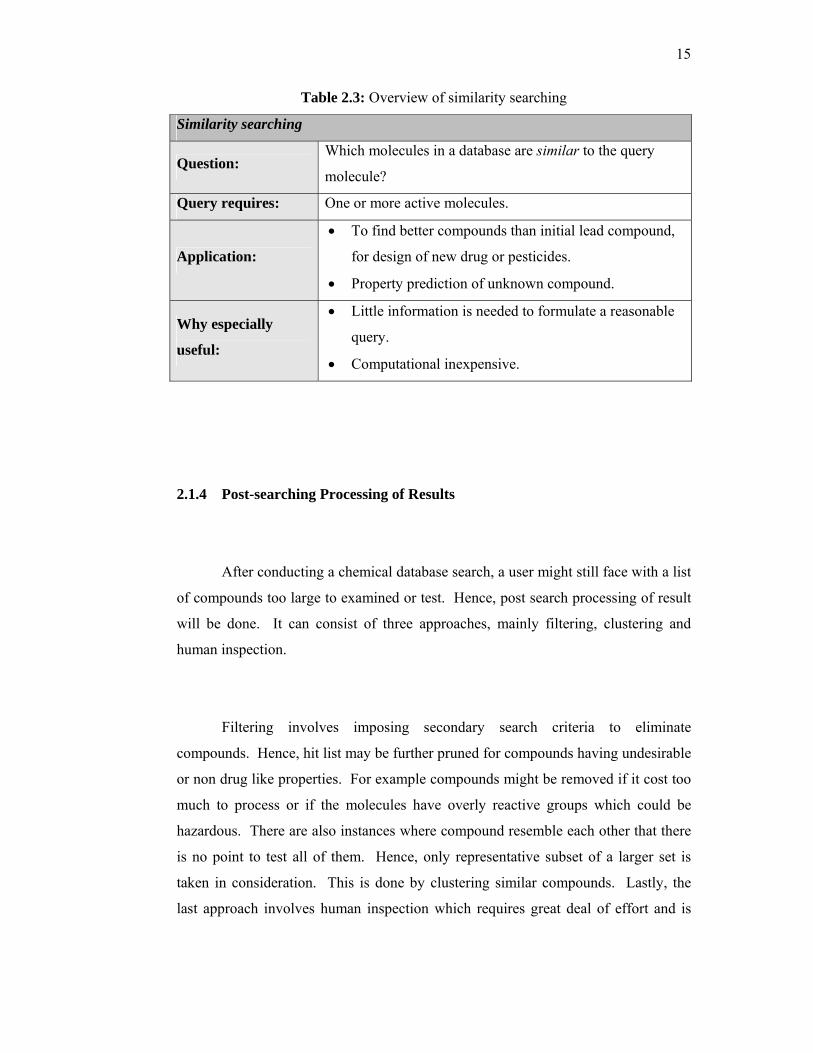
Table 2.3: Overview of similarity searching
Similarity searching
Question: Which molecules in a database are similar to the query
molecule?
Query requires: One or more active molecules.
Application:
• To find better compounds than initial lead compound,
for design of new drug or pesticides.
• Property prediction of unknown compound.
Why especially
useful:
• Little information is needed to formulate a reasonable
query.
• Computational inexpensive.
2.1.4 Post-searching Processing of Results
After conducting a chemical database search, a user might still face with a list
of compounds too large to examined or test. Hence, post search processing of result
will be done. It can consist of three approaches, mainly filtering, clustering and
human inspection.
Filtering involves imposing secondary search criteria to eliminate
compounds. Hence, hit list may be further pruned for compounds having undesirable
or non drug like properties. For example compounds might be removed if it cost too
much to process or if the molecules have overly reactive groups which could be
hazardous. There are also instances where compound resemble each other that there
is no point to test all of them. Hence, only representative subset of a larger set is
taken in consideration. This is done by clustering similar compounds. Lastly, the
last approach involves human inspection which requires great deal of effort and is

16
very time-consuming. However, it may yield valuable results drawn from insights
after seeing a set of structures in the wider context of the research process.
2.2 Representation of Chemical Structures
Selecting compounds requires some quantitative measure of similarity
between compounds. These quantitative measures in turn depend on the compound
representation or structural descriptors that are amenable to such comparisons.
Structural descriptors are actually vectors of numbers, where each of them is based
on some-predefined attributes. They are generated from a machine-readable
structure representation like a 2D connection table or a set of experimental or
calculated 3D coordinates. Molecular descriptors can be classified into 1-
dimensional (1D), 2-dimensional (2D) and 3-dimensional (3D) descriptors.
2.2.1 1D Descriptors
1D descriptors model 1D aspect of molecules. It is also known as global
molecular properties where physicochemical properties are used as molecular
descriptors. Examples of these properties are molecular weight, ClogP (log of the
octanol / water partition coefficient), molar refractivity (the ratio of the speed of light
in a vacuum to its speed in a sample compound) and many more. The main
disadvantage of physicochemical properties is that they need to be calculated for
every compound in the database and some properties can be extremely time-
consuming to calculate.
17
2.2.2 2D Descriptors
2D descriptors model 2D aspects of molecule obtained from the traditional
2D structure diagram. There are two types of 2D descriptors which are the
topological indices and 2D screens. Topological indices characterise the bonding
pattern of a molecule by a single value integer or real number. The value obtained is
from mathematical algorithms applied to the chemical graph representation of
molecules. Thus, each index contains information not about fragments or some
locations on the molecule, but rather about the molecule as a whole. The second type
of 2D descriptors is the 2D screens, which is the focus of this project and thus
explained in detailed in this section.
2D screens refer to bit strings that are used to represent molecules. It was
originally developed for substructure search system. 2D screens can be further
classified to dictionary-based bit strings and hashed fingerprints. In dictionary-based
bit strings, a molecule is split up into fragments of specific functional groups or
substructure. Substructural fragments can involve atoms, bonds and rings. Example
of fragment types used in 2D screens can be seen in Figure 2.1.
Fragment are recorded in a predefined dictionary of fragments, that specifies
the corresponding bit position or screen number of the fragments in the bit string. If
a particular fragment is present, then a corresponding bit is set in the bit string. The
number of occurrence of the fragment is not recorded in the bit string. Hence if a
fragment is present for 100 times, it would only set one bit. It is the number of
different types of fragments that determines the number of bits set in a bit string and
not its quantity. Examples of dictionary based bit strings are BCI bit strings (Barnard
Chemical Information Ltd.) and MDL MACCS key system (Durant, et al., 2002).
Figure 2.2 shows the concept of encoding chemical structure as a bit string.

18
Figure 2.1 Example of fragment types used in 2D screens (Salim, 2002)
Figure 2.2 Encoding chemical structure as a bit string (Flower, 1997)
Another alternative to dictionary-based bit strings is hashed fingerprint.
Unlike the previous bit string, it is not dependent on a predefined list of structural

19
fragments. Instead, unique fragments that exist in a molecule are hashed using some
hashing function to fit into the length of the bit string. Hence, the fingerprints
generated are characterized by the nature of the chemical structures in the database
rather than by fragments in some predefined list.
Hashed fingerprint adopt the path approach to replace fragment dictionary.
By default, all paths through the molecular graph of length 1 to 8 atoms are found.
Bits corresponding to each possible type of path are set if present. The resulting bit
string is then folded to reduce storage requirements and speed searching. Example of
system using hashed fingerprints is the Daylight Chemical Information system
(James, et al., 2000). Figure 2.3 shows how bits are set using this approach. A
molecule is decomposed into a set of atom paths of all possible lengths. Each of
these paths is then mapped to a bit set in a corresponding binary string. Although all
existing fragments are included in the hashed fingerprint, it can result in very dense
fingerprints. Overlapping of patterns as a result from hashing can also cause loss of
information and give false similarity values, as common bits in two strings can be set
by completely unrelated fragments.
Figure 2.3 Bits set using the path approach (Flower, 1997)
20
Currently, 2D screens are widely used for database searching, mainly on
selecting compounds for inclusion in biological screening programs. This is due to
its proven effectiveness (Brown and Martin, 1997), and low processing requirements
to calculate similarities between a target structure and large number of structures.
2.2.3 3D Descriptors
3D descriptors model 3D environment of molecules. They have the ability to
model the biological activity of molecules because the binding of a molecule to a
receptor site is a 3D event. Examples of 3D descriptors are 3D screens, Potential-
Pharmocophore-Point (PPP) and affinity fingerprints. 3D descriptors however, are
computationally more expensive than 2D descriptors. This is because, it does not
only involve generating 3D structure but it needs also to handle conformational
flexibility and decide which conformers to include. Brown and Martin (1997) also
state that 3D fingerprints are not generally superior to 2D representation and that
complex designs do not necessarily perform better than simpler ones.
2.3 Similarity Coefficients
One of the most important components of a similarity searching system is the
measure that is used to quantify the degree of structural resemblance between the
target structure and each of the structures in the database. This measure is called
similarity coefficients. This section gives brief overview on types of coefficients
used in the chemical database searching, with some common examples. Although
there are many ways in expressing similarity coefficient, discussion is limited to the

21
binary form of the coefficient since this project involves the usage of 2D bit string
based similarity measures.
Assume that a chemical structure, SM is described by listing its set of binary
attribute-values or vector, such that SM = {b1M, b2M, b3M, … bnM}, where there are n
attributes, and biM is the value of attribute Ai for structure SM. The coefficients shown
in this section are in binary form, where the presence or absence of bit Ai in the set of
bits, is used to represent chemical structures SM or query SQ. SimM, Q is the similarity
between molecule M and query molecule Q. There are two ways of expressing the
formulae of similarity coefficients, when the data under analysis is in binary form:
a) Formulae based on the 2 x 2 contingency table
Based on Table 2.4, a is equal to the number of attributes whose value
both in SM and in SQ is 1, while d is equal to number of attributes whose
value both in SM and in SQ is 0. b is equal to the number of attributes
whose value in SM is 1 and in SQ is 0 while c is equal to the number of
attributes whose value in SM is 0 and in SQ is 1. The sum of all these
value (a + b + c + d) is equal to the number of attributes, n of each
chemical structure. The examples shown in this section uses 2 x 2
contingency table to express the similarity coefficients.
Table 2.4: 2 x 2 contingency table biQ = 1 biQ = 0
biM = 1 a b
biM = 0 c d
b) Formulae based on set theory
A second alternative is to use the set-theoretic notation, where the
following are defined:
22
sm is the set elements biM in vector SM whose value is 1,
sq is the set elements biQ in vector SQ whose value is 1,
| sm | refers to the number of elements in set sm,
| sq | refers to the number of elements in set sq,
| sm ∩ sq | refers to the number of elements common to both sm
and sq,
| sm ∪ sq | refers to the number of elements in both sm and sq.
|sm ∩ sq| in this notation is equivalent to a in the previous notation and
|sm ∪ sq| is equivalent to n. | sm | is equivalent to a + b and | sq | is
equivalent to a + c. Hence, we can easily convert from one notation to
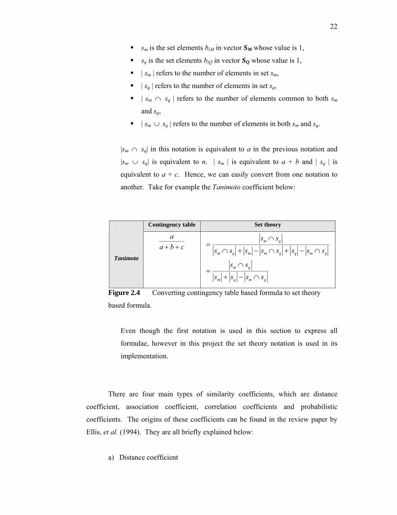
another. Take for example the Tanimoto coefficient below:
Contingency table Set theory
Tanimoto
cbaa++
qmqm
qm
qmqqmmqm
qm
ssss
ss
ssssssss
ss
∩−+
∩=
∩−+∩−+∩
∩=
Figure 2.4 Converting contingency table based formula to set theory
based formula.
Even though the first notation is used in this section to express all
formulae, however in this project the set theory notation is used in its
implementation.
There are four main types of similarity coefficients, which are distance
coefficient, association coefficient, correlation coefficients and probabilistic
coefficients. The origins of these coefficients can be found in the review paper by
Ellis, et al. (1994). They are all briefly explained below:
a) Distance coefficient

23
This coefficient is used to measure the distance between structures in a
molecular space. It is difficult to visualise the geometry of a space of
more than 3 dimensions (hyperspace). Hence to preserve the validity of
geometric distances between objects in a hyperspace, the coefficient must
have the property of metrics. In order to do so, a distance coefficient
needs to obey certain rules:
Distances must be zero or positive: SimM, Q ≥ 0
Distances from object to itself must be zero: SimM, Q = SimQ, M =
0
Distance between non-identical objects must be greater than zero:
If SM ≠ SQ, then SimM, Q > 0
Distance must be symmetric: SimM, Q = SimQ, M
Distance must obey the triangular inequality: SimM, Q ≤ SimM, X +
SimQ, X
Table 2.5: Examples of distance coefficients (Ellis, et al., 1994)
Coefficient Binary Formula
Mean Manhattan
ncb +
Mean Euclidean
ncb +
Mean Canberra
ncb +
Divergence
ncb +
b) Association coefficient
Association coefficient is a pair-function that can measure the agreement
between the binary, multi-state or continuous character representations of
two molecules. It is based on the inner product of corresponding
elements of two vectors denoted by a. The basic formula of an

24
association coefficient for binary data is formed by dividing a. The
following table shows examples of association coefficients:
Table 2.6: Examples of association coefficients (Ellis, et al., 1994)
Coefficient Binary Formula
Jaccard / Tanimoto
cbaa++
Ochiai / Cosine
))(( cabaa
++
Dice
cbaa++2
2
Russell / Rao
na
Sokal / Sneath
c2b2aa++
c) Correlation coefficient
This coefficient measures the degree of correlation between sets of values
representing the molecules, like the proportionality and independence
between pairs of real-valued molecular descriptors. The following table
shows examples of correlation coefficients:
Table 2.7: Examples of correlation coefficients (Ellis, et al., 1994)
Coefficient Binary Formula
Pearson
))()()(( dcdbcababcad
++++−
Yule
bcadbcad
+−
McConnaughey
))(( cababca 2
++−
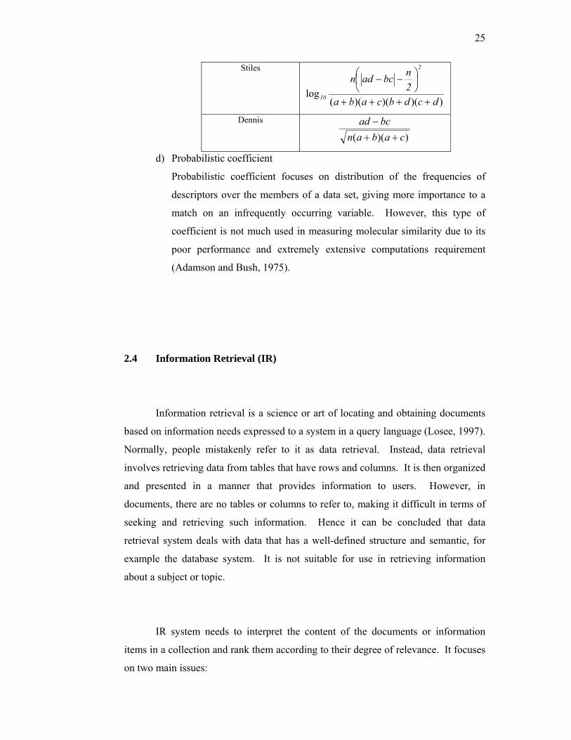
25
Stiles
))()()((log
dcdbcaba2nbcadn
2
10 ++++
⎟⎠⎞
⎜⎝⎛ −−
Dennis
))(( cabanbcad
++−
d) Probabilistic coefficient
Probabilistic coefficient focuses on distribution of the frequencies of
descriptors over the members of a data set, giving more importance to a
match on an infrequently occurring variable. However, this type of
coefficient is not much used in measuring molecular similarity due to its
poor performance and extremely extensive computations requirement
(Adamson and Bush, 1975).
2.4 Information Retrieval (IR)
Information retrieval is a science or art of locating and obtaining documents
based on information needs expressed to a system in a query language (Losee, 1997).
Normally, people mistakenly refer to it as data retrieval. Instead, data retrieval
involves retrieving data from tables that have rows and columns. It is then organized
and presented in a manner that provides information to users. However, in
documents, there are no tables or columns to refer to, making it difficult in terms of
seeking and retrieving such information. Hence it can be concluded that data
retrieval system deals with data that has a well-defined structure and semantic, for
example the database system. It is not suitable for use in retrieving information
about a subject or topic.
IR system needs to interpret the content of the documents or information
items in a collection and rank them according to their degree of relevance. It focuses
on two main issues:
26
a) Extracting the semantic information from the document text,
b) Match it with user’s request and determine their degree of relevance.
Recently, IR has taken the centre stage. Before the World Wide Web
(WWW) is introduced, finding and retrieving information has depended on an
intermediary such as librarians or other information experts. This field used to be
considered as too esoteric for a typical user. The Web is an enormous repository of
knowledge and culture. Now, every group of users can use it to find information. Its
success is due to its standard user interface that hides the computational environment
running it. Since the Web is vast and unknown, how does one find information?
Surely by navigating through the Web would be a tedious and inefficient way of
doing it.
Matters are made worst when there is no well-defined underlying data model
for the Web. Hence, IR research is now an important component in major
information services and the Web. Its goal is to facilitate convenient retrieval of
information regardless of its form, medium or location.
2.4.1 Retrieval Process
To show how retrieval is done, consider the following example. Below is a
user information need:
Find all documents containing information on the crime rate in Kuala
Lumpur involving teenagers.
In order to be relevant, the result must include statistic of crime rates in Kuala
Lumpur that only involves teenagers. The user must then translate this information
into a query, which can be processed by the IR system. Translation usually produces

27
set of keywords or index terms, which represent the description of the user’s
information need.
IR system then retrieve document which might be useful or relevant to the
user, ranking it according to a likelihood of relevance, before showing it to the user.
Normally, the results will not be good, as most users do not know how to formulate
their query out of their information needs.
The user then examines the set of ranked documents for useful information.
At this point, user can pinpoint a subset of useful document and initiate a user
feedback cycle, which is based on the documents selected by the user. The system
then changes the query formulation. This modified query is a better representation of
the user’s need and hence, a better retrieval.
2.4.2 Classical Retrieval Model
In IR models, the following elements are given:
a) A finite set of identifier (e.g. keyword, terms)
b) A finite set of documents where a document can be a collection of some
other objects or modelled as a series of weights. Weights refers to the
degree to which identifier relate to a particular document.
c) A finite set of criteria (e.g. relevance, non-relevance), according to which
two documents are compared to each other. The result of this comparison
is a score assigned to that pair of documents.

28
Classical retrieval is a process of associating documents to a query, which the
scores are greatest, based on a given criterion (Dominich, 2000). As described
earlier, IR involves documents, denoted by d and a given query, q. Retrieval
involves the task of finding these documents, which implies the query (d→q).
Initially, Boolean retrieval model was used to do this task. A review of this
model as well as other classical retrieval models can be found in Fuhr (2001).
Boolean model is part of the exact matching methods category, where the query are
normally represented by Boolean statements, consisting of search terms interrelated
by the Boolean operators AND, OR and NOT. The retrieval system will then select
those stored items that are identified by the exact combination of search terms
specified by the query. Given a four-term query statement such as “(A AND B) OR
(C AND D)”, the retrieved items will contain either the term pair A and B or the pair
C and D or both pairs.
Retrieval performance of the Boolean model depends on the type of search
request submitted and on the homogeneity of the collection being searched (Blair and
Maron, 1985). Specific queries may lead to only a few items being retrieved but are
most likely to be useful. On the other hand, when query are broadly formulated,
many more stored items are retrieved, including both relevant and irrelevant items.
Retrieval performance is also generally better when the stored collection covers a
well-defined subject, compared to those covering many different topic areas.
This model has been widely accepted, because Boolean formulations can be
used to express term relationships such as synonym relations identified by the OR
operators and term phrases specified by the AND operators. Furthermore, fast
responses are obtained even for very large document collections.

29
Unfortunately, Boolean model posses some disadvantages. Firstly, all
retrieved documents are assumed to be equally useful. This approach also has no
ranking system. Thus it acts more like a data retrieval model rather than an IR
model. Secondly, successful retrieval mainly requires a very well formed query and
good search keys. This is not likely since that the users have problem specifying
their information needs. The document representations itself are imprecise, since IR
system has only limited processing methods that can represent the semantics of a
document. Certainly, this would lead to retrieval of too few or too many documents.
Thus, IR research turns to partial match methods category to overcome the
limitation of the Boolean approach. It consists of two retrieval models that is Vector
Space Model (VSM) and Probability Model (PM). VSM is based on index term
weighting. These term weights are used to compute the degree of similarity between
each documents stored in the system and the user query. Then, the retrieved
documents are sorted in decreasing order of this degree of similarity. PM on the
other hand, captures the IR problem within a probabilistic framework. The model
tries to estimate the probability that the user will find the document interesting or
relevant. It then presents to the user ranked documents in decreasing order of their
probability of relevance to the query. In contrast to the Boolean model, both of these
approaches take into consideration documents, which match the query term only
partially. As a result, the ranked documents retrieved, are more precise than the
documents retrieved by the Boolean model (Yates and Nato, 1999). The following
sections explain these models in more detail.
2.5 Vector Space Model (VSM)
The VSM (Salton and Buckley, 1988a), represents both the documents and
queries as a vector of terms. Given a document Dj and a query q characterised by a
30
vector, such that Dj = {t1j, t2j, t3j, ..., tnj} and q = {t1q, t2q, t3q, ..., tnq}, where there are n
elements. Elements tij or tiq is a value representing either:
a) The presence or absence of term ti in the set of terms that is used to
represent document Dj or query q in which the data are in binary form.
Here, every term is treated equally. One may argue that this does not
reflect real life situation, where one term may have more importance than
others. Hence, the second approach is being employed as explained
below.
b) The weight of term ti in the set of terms that is used to represent
documents Dj or query q, in which data are in non-binary form. Here,
term weights are used to distinguish the degree of importance of the
terms.
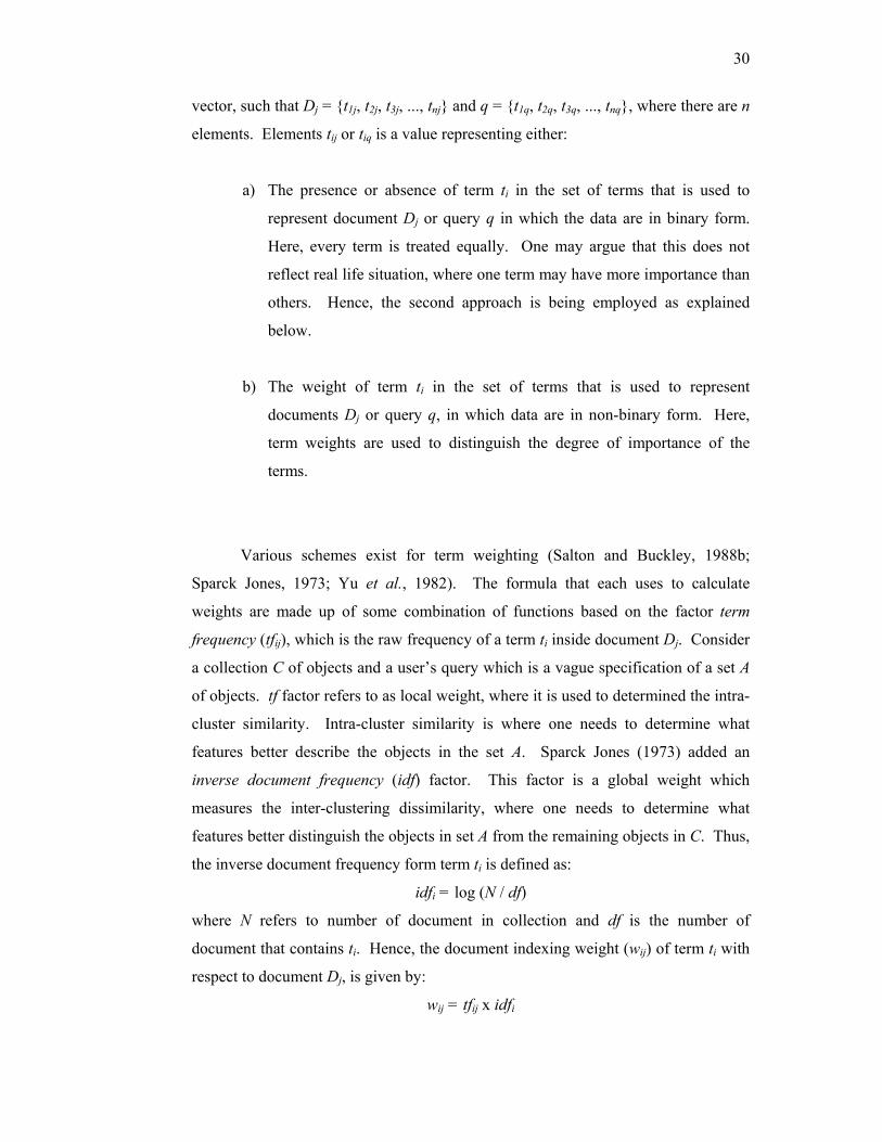
Various schemes exist for term weighting (Salton and Buckley, 1988b;
Sparck Jones, 1973; Yu et al., 1982). The formula that each uses to calculate
weights are made up of some combination of functions based on the factor term
frequency (tfij), which is the raw frequency of a term ti inside document Dj. Consider
a collection C of objects and a user’s query which is a vague specification of a set A
of objects. tf factor refers to as local weight, where it is used to determined the intra-
cluster similarity. Intra-cluster similarity is where one needs to determine what
features better describe the objects in the set A. Sparck Jones (1973) added an
inverse document frequency (idf) factor. This factor is a global weight which
measures the inter-clustering dissimilarity, where one needs to determine what
features better distinguish the objects in set A from the remaining objects in C. Thus,
the inverse document frequency form term ti is defined as:
idfi = log (N / df)
where N refers to number of document in collection and df is the number of
document that contains ti. Hence, the document indexing weight (wij) of term ti with
respect to document Dj, is given by:
wij = tfij x idfi

31
In this model, both document and query representations are described as
points in T dimensional space, where T is the number of unique terms in the
document collection. Figure 2.5 shows an example of a VSM representation for a
system with three terms.
Figure 2.5 Three dimensional vector space.
Each axis in the space corresponds to a different term. The position of each
document vector in the space is determined by the weight of the terms in that vector,
which is discussed previously. Here, there is just one criterion considered, which is
relevance. Similarity between query and document is measured by a function that
determines the matching terms in the respective vectors in order to identify the
relevant documents. This function is also referred to as the similarity measure which
has three basic properties:
a) It has a value between 0 to 1,
b) It does not depend on the order of which the document are being
compared, and
c) If the value is equal to 1, then the query vector is the same as the
document vector.
q
D2
Term1
Terms2
Terms3
D1

32
A common example of similarity measure is the Cosine coefficient, which
evaluate the degree of similarity of document with regards to the query q, as the
distance between the vector Dj and q. This distance can be quantified by using the
cosine angle between there two vectors, which is given below:
∑∑
∑
==
=
×
×=
t
1j
2iq
t
1i
2ij
t
1iiqij
j
ww
wwqDSim
)()(),(
Based on this explanation, we can determine that in Figure 2.5, the
documents D2 is more similar to the query q, due to its distance being nearer to q
compared to D1. Other than the Cosine coefficient, there are also other similarity
measures used in text retrieval as listed by Ellis, et al. (1994).
Values obtained from the similarity measures are next used to produce ranked
list of relevant document. They are sorted in decreasing order of the measures.
Documents are said to be retrieved if their similarity measures exceeding a threshold
value which is normally requested from the user.
The VSM is a popular retrieval model especially among the Web community.
It is either superior or almost as good as other alternative (Yates and Nato, 1999).
This is due to its approach that is known for being simple and very effective in
retrieving information. The following is the rest of the main advantages of this
model:
a) Documents are ranked according to their degree of similarity to the query.
b) Partial matching strategy allows retrieval of documents that approximate
the query condition.
c) Term weighting scheme improves retrieval performance.

33
However, the model is not without its drawbacks. The disadvantages of this
model are stated below:
a) In VSM, terms are assumed to be mutually independent, for example the
following figure. Assume that a complete concept space, U is form by a
set of terms: 4321 ttttU ∪∪∪= . The term t corresponds to the disjoint
basic concepts: ti ∩ tj = Ø for i ≠ j. As a result, terms form a dissection of
U. However, in practice, terms are not necessarily independent of all
other terms.
Figure 2.6 Disjoint concept of U
b) Even though this model is simple, its ranked answer sets are difficult to
improve on without query expansion or relevance feedback within the
framework of the vector model (Yates and Neto, 1999).
2.6 Probability Model (PM)
In the PM, formal probability theory and statistics are used to estimates the
probability of relevance by which the document are ranked. This methodology is to
t1 t2
t3 t4

34
be distinguished from looser approaches like the VSM, in which the retrieved items
are ranked by a similarity measures whose values are not directly interpretable as
probabilities.
Given a document (D), a query (q) and a cut-off numeric value of
probability., this model computes the conditional probability P(D|R) that a given
document D is observed on a random basis given relevant event R, that the document
is relevant to the query (van Rijsbergen, 1979). Query and document are represented
by a set of terms. Then P(D|R) is calculated as a function of the probability of
occurrence of these terms in relevant against non-relevant documents. The term
probabilities are similar to the term weights in the VSM. However, a probabilistic
formula is used to calculate P(D|R), in place of the similarity coefficient used to
calculate relevance ranking in VSM. The probabilistic formula depends on the
specific model used, and also on the assumptions made about the distribution of
terms. An overview of the many probabilistic models developed can be seen in
Crestani, et al. (1998). This project however focuses on only two models as
explained in later sections (BIR and BD models).
Next, documents with relevance probability exceeding its non-relevance
probability are ranked in decreasing order of their relevance. Documents are said to
be retrieved when their relevance probability exceed the cut-off value. According to
the Probability Ranking Principle (PRP), retrieval system effectiveness is optimal if
documents are ranked according to their probability of relevance. The justification
of this system principle is as follows: Let C denotes the cost of retrieving a relevant
document and C as costs for retrieving a non-relevance document. A user prefers
relevant documents, and thus CC > is assumed. Then the expected cost (EC) for
retrieving a document D is computed as:
where P(R|D) refers to the probability of relevant documents and 1- P(R|D) =
P(NR|D) refers to probability of non-relevant documents.
))|(1()|()( DRPCDRPCDEC −⋅+⋅=
35
In a ranked list of documents, a user will look at the document and stops at an
arbitrary point. In order to minimize the sum of expected cost at any cut-off point,
documents have to be ranked in the order of the increase of expected cost. For
example, for any two documents D1 and D2, rank D1 ahead of D2 if EC(D1) <
EC(D2). Due to CC > , this condition is equivalent to P (R | D) > P (NR | D).
Hence, documents are ranked to decreasing probability of relevance, in order to
minimize the expected cost. So, here it can be seen that probabilistic retrieval
models are directly related to retrieval quality.
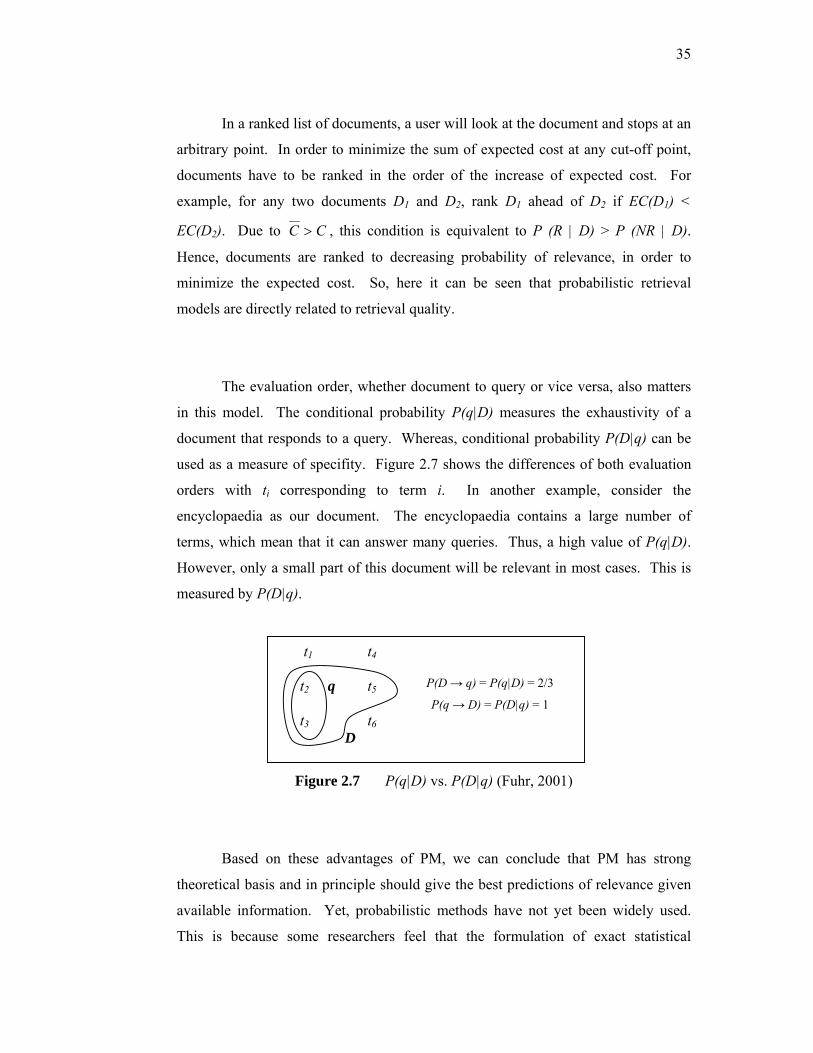
The evaluation order, whether document to query or vice versa, also matters
in this model. The conditional probability P(q|D) measures the exhaustivity of a
document that responds to a query. Whereas, conditional probability P(D|q) can be
used as a measure of specifity. Figure 2.7 shows the differences of both evaluation
orders with ti corresponding to term i. In another example, consider the
encyclopaedia as our document. The encyclopaedia contains a large number of
terms, which mean that it can answer many queries. Thus, a high value of P(q|D).
However, only a small part of this document will be relevant in most cases. This is
measured by P(D|q).
Figure 2.7 P(q|D) vs. P(D|q) (Fuhr, 2001)
Based on these advantages of PM, we can conclude that PM has strong
theoretical basis and in principle should give the best predictions of relevance given
available information. Yet, probabilistic methods have not yet been widely used.
This is because some researchers feel that the formulation of exact statistical
t1 t4 t2 q t5 t3 t6 D
P(D → q) = P(q|D) = 2/3
P(q → D) = P(D|q) = 1

36
assumptions is an unnecessary theoretical burden. They would rather spend the time
and effort on looser formalisms and simpler approach than the probability theory.
There is also the need to guess the initial separation of documents into relevant and
non-relevant sets, and ongoing training collection with relevance information in
order to provide clues about the documents when computing the conditional
probability P(D|R).
2.6.1 Binary Independence Retrieval (BIR) Model
The BIR model (van Rijsbergen, 1979; Fuhr, 1992) is the simplest of all
probabilistic models. It is based on the presence or absence of independently
distributed terms in relevant and non-relevant documents. This means that the
probability of any given term occurring in a relevant document is independent of the
probability of any other term occurring in a relevant document and similarly for non-
relevant documents. Hence, the name Binary Independence.
This model takes into account the non-disjoint concepts, where with term ti
and tj, ti ∩ tj ≠ Ø. Hence, terms are map onto disjoint atomic concept by forming
conjuncts of all term t, in which each term either occurs positively or negated.
Hence, a document, D is represented as:
n1n1 ttD αα ∩∩= ... with =i
itα
⎩⎨⎧ =
=1 if t0 if t
ii
ii
αα
ti refers to the term t at location i on the document vector. Whereas, αi acts as
a binary selector that is, if αi = 1, then it means that the term occurs in the document,
otherwise it is 0 and assumed negated. For example, consider the following diagram,
which illustrates a disjoint concept of three terms namely t1, t2 and t3, with Di,
referring to documents. The complete conjuncts of terms are as follows:

37
32173216
32153214
32133212
32113210
tttD tttD
tttD tttD
tttD tttD
tttD tttD
∩∩=∩∩=
∩∩=∩∩=
∩∩=∩∩=
∩∩=∩∩=
Figure 2.8 Construction of disjoint concepts for the case of 3 terms
2.6.1.1 Retrieval Status Value (RSV)
Retrieval status value refers to the similarity function that estimates ranking
score of a particular document against the query posted by the user. The optimal
ranking function is given as P(R|D) / P(NR|D). P(R|D) refers to the conditional
probability of relevant documents whereas P(NR|D) refers to the conditional
probability of non-relevant documents. In order to estimate the probability of
relevant and non-relevant documents, we consider the Bayes theorem where:
)()|()()|(
)()|()()|(
DPNRDPNRPDNRP
DPRDPRPDRP
⋅=
⋅=
(2.1)
D1 D2
D3
D4
D7
D6 D5
D0
t1 t2
t3

38
P(D|R) is the probability of a relevant document,
P(D|NR) is the probability of a non-relevant document,
P(R) is the probability of relevance,
P(NR) is the probability of non-relevance,
where
P(D) is the probability of the document.
Thus, by substituting the optimal ranking function with the expression in
(2.1), we get:
)|()()|()(
)|()|(
NRDPNRPRDPRP
DNRPDRP
⋅⋅
= (2.2)
Efficient matching requires data on the terms presence or absence in
documents. Other than that, it also requires terms presence probabilities in relevant
and non-relevant documents. Hence, two variables were defined, which are:
a) pi that refers to the probability that a term appearing in a relevant
document (R). The complement of pi, denotes the probability of absence
of a term in R.
b) qi that refers to the probability that a term appearing in a non-relevant
document (NR). The complement of qi, denotes the probability of
absence of a term in NR.
Let αi refers to as a binary selector, as mentioned before. Now, the
probability of relevance of a document P (D|R) is given as: ii 1
in1i i p1pRDP αα −=
−=∏ )()()|(..
where pi = P (αi = 1 | R) and (1-pi) = P (αi = 0 |R). Whereas, the probability of non-
relevance of a document P (D | NR) is given as: ii 1
in1i i q1qNRDP αα −=
−=∏ )()()|(..

39
where qi = P (αi = 1 | NR) and (1-qi) = P (αi = 0 |NR).
Thus, by substituting both the above expression in (2.2), the ranking function
becomes:
)()(
)()(
)|()|(
.. NRPRP
q1p1
p1qq1p
DNRPDRP
i
in1i
ii
iii
⋅⎟⎟⎠
⎞⎜⎜⎝
⎛−−
⋅⎟⎟⎠
⎞⎜⎜⎝
⎛−−
=∏ =
α
(2.3)
Then, by taking the logs of the ranking function, it will transform (2.3) into a
linear discriminate function:
∑
∑
∑
∩∈
=
=
=
+=
+⎟⎟⎠
⎞⎜⎜⎝
⎛−−
+⎟⎟⎠
⎞⎜⎜⎝
⎛−−
=
qDbi
n
1ii
i
i
ii
iin
1ii
i
ic
Cic
NRPRP
q1p1
p1qq1p
DNRPDRP
α
α
α)(
)(loglog)()(log
)|()|(
(2.4)
The constant C, which has been assumed the same for all documents, will
vary from query to query. It can be interpreted as the cut-off value applied to the
retrieval function. ci indicates the capability of a term to discriminate relevant from
the non-relevant document. It is also referred to as relevance weights or term
relevance.
2.6.1.2 Probability estimation and improvement
There are two instances in probability estimation. If we already know the set
of relevant documents R, ci can be interpreted with assistance of the following table.
Let N be the number of documents in the database and R refers to the number of
relevant documents. n refers to the number of documents which contain term ti,
whereas r refers to the number of relevant documents which contain term ti.

40
Table 2.8: Contingency table for estimating ci (van Rijsbergen, 1979)
Relevant Non-relevant
αi = 1 r n-r n
αi = 0 R-r N-n-R+r N-n
R N-R N
pi can be estimated as r/R whereas qi can be estimates as (n-r) / (N-R).
Hence, the ci can be rewritten as:
))(()(log
rRrnrnRNrci −−
+−−=
The last formula for pi and qi can create problems for small values of R and ri
which normally is the case in real situation (Yates and Neto, 1999). To avoid these
problems, an adjustment factor is often added in which yield:
a) pi = (ri + 0.5) / (R + 1)
b) qi= (ni - ri + 0.5) / (N – R + 1)
The second instance in estimating probability of pi and qi is when we do not
know the set of relevant documents R at the beginning. Hence, it is necessary to
devise a method for initially computing the probabilities P(D|R) and P(D|NR). In the
beginning, they are no retrieved documents. Thus, the following assumption is
made:
a) pi is assumed a constant for all index term ti. Usually, the value 0.5 is
selected:
pi = 0.5
41
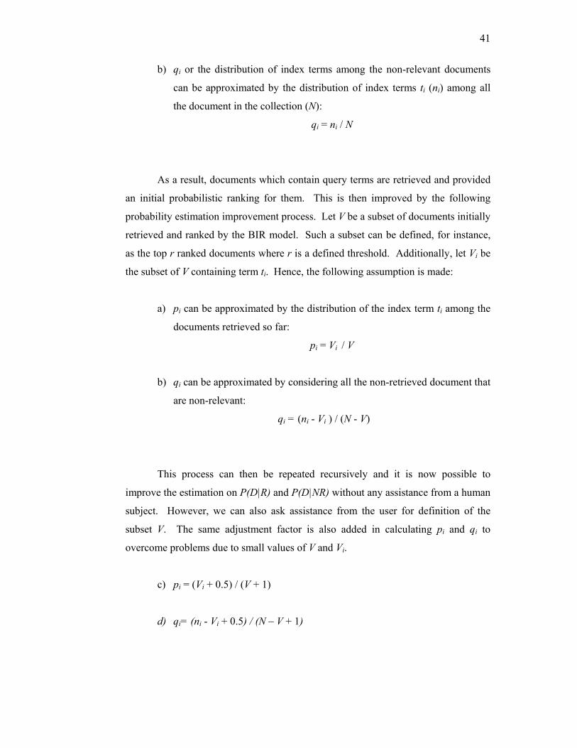
b) qi or the distribution of index terms among the non-relevant documents
can be approximated by the distribution of index terms ti (ni) among all
the document in the collection (N):
qi = ni / N
As a result, documents which contain query terms are retrieved and provided
an initial probabilistic ranking for them. This is then improved by the following
probability estimation improvement process. Let V be a subset of documents initially
retrieved and ranked by the BIR model. Such a subset can be defined, for instance,
as the top r ranked documents where r is a defined threshold. Additionally, let Vi be
the subset of V containing term ti. Hence, the following assumption is made:
a) pi can be approximated by the distribution of the index term ti among the
documents retrieved so far:
pi = Vi / V
b) qi can be approximated by considering all the non-retrieved document that
are non-relevant:
qi = (ni - Vi ) / (N - V)
This process can then be repeated recursively and it is now possible to
improve the estimation on P(D|R) and P(D|NR) without any assistance from a human
subject. However, we can also ask assistance from the user for definition of the
subset V. The same adjustment factor is also added in calculating pi and qi to
overcome problems due to small values of V and Vi.
c) pi = (Vi + 0.5) / (V + 1)
d) qi= (ni - Vi + 0.5) / (N – V + 1)

42
2.6.2 Binary Dependence (BD) Model
Most IR models assume terms of query and documents are independent from
each another. This assumption of terms independence is a matter of mathematical
convenience and hence yields to simplistic retrieval system. Research work by
Bollmann-Sdorra and Raghavan (1998) showed that, for retrieval functions such as
the cosine used in the VSM, weighted retrieval is incompatible with term
independence in query space. They also proved that the term independence in the
query space even turned out to be undesirable.
The hazard of term independence is also pointed out by Cooper (1995),
mainly on data inconsistency. He also stated that the BIR model, discussed in the
previous section, is mistakenly named and better referred to as linked-dependence
model. This model has been called Binary Independence, because simplified
assumption is made, where document properties that serve as clues to relevance are
independent of each other in both set of relevant documents and the set of non-
relevant documents. However, Cooper stated that BIR model does exhibit weaker
link-dependence. Although this is very much debatable, it has at least the virtue of
not denying the existence of dependencies. Link-dependence is based on one
important assumption:
)|()|()|()|(
)|,()|,(
NRBPNRAPRBPRAP
NRBAPRBAP
=
where A, B are regarded as properties of documents and R designates the relevance
set whereas NR designates the non-relevance set. The degree of statistical
dependence of documents in the relevant set is associated in a certain way with their
degree of statistical dependence in the non-relevant set.
Hence, the correct procedure is to assume dependence of terms and thus
creating a more realistic retrieval system. Term dependencies exist when the
relationships between terms in document are such that the presence or absence of one
term provides information about the probability of the presence or absence of another

43
term (Loose, 1994). Based on this assumption, many probabilistic models were
proposed to remove the independence assumption. For example, the Bahadur
Lazarsfeld Expansion or BLE (Losee, 1994) and tree dependence model (van
Rijsbergen, 1979). The tree dependence model exhibits a number of advantages over
the exact model provided by the BLE expression. It is also more easily computed
than the BLE expansion (Salton, et al., 1983). Tree dependence model applies the
approach suggested by Chow and Liu (1968) to capture term dependence, where an
MST is constructed using mutual information, for a dependence tree. Also from this
approach is the Chow Expansion, which was originally used in the pattern
recognition field. However, it has been applied in probabilistic IR as done by Lee
and Lee (2002) and hence will be the focus of this project.
Instead of just considering the absence or presence of individual terms
independently, one selects certain pairs of terms and calculates a weight for them
jointly. Assume vector D = {t1, t2 . . . tn} are binary values. Dependence can be
arbitrarily complex as follows:
)...,|()...,|()|()()...()( 1nt2t1tntP2t1t3tP1t2tP1tPnt1tPDP −== (2.5)
in which we need to condition each variables in turn by steadily increasing set of
other variables, to capture all dependence data. This is computationally inefficient
and impossible if we do not have sufficient data to calculate the high order
dependencies. Hence, another approach is taken to estimate P(D), which captures
the significant dependence information. P (ti | ti-1 … t1) is solely dependent on some
preceding variable tj(i). In other words, we obtained:
ij(i)0 n
1i ijtitPDP ≤≤∏=
= ))(|()( (2.6)
A probability distribution that can be represented as in the above expression
is called a probability distribution of first-order tree dependence (Chow and Liu,
1968). For example the Figure 2.9, according to equation (2.6), the probability of a
structure can be written as P(t1) P(t2|t1) P(t3|t2) P(t4|t2) P(t5|t2), or the following
product expansion:

44
P(t1)P(t2|tj(2)) P(t3|tj(3))… P(tn|tj(n))
where the function j(i) exhibits the limited dependence of one bit on preceding bits.
Figure 2.9 Term dependence tree
2.6.2.1 Dependence Tree
A dependence tree is an obvious method for identifying the most important
pairwise dependencies and the best mapping of j(i). Chow and Liu (1968) suggest
constructing a Maximum Spanning Tree or MST (Whitney, 1972). The nodes are
used to represent the individual terms and the branches between pairs of nodes,
which designates the pair wise similarities or dependencies. To construct an MST
for a set of entities, we need to identify the most important similarities between pairs
of entities. Expected Mutual Information Measure or EMIM is a criterion for
measuring this similarity or dependence between pairs (Crestani et al., 1995).
Hence, an MST is a tree that includes every node and maximizes the sum of EMIM.
EMIM is defined as follows:
∑=
jtit jtpitPjtitP
jtitPjtitI, )()(
),(log),(),(
t1
t2
t3 t4 t5

45
where the sum is taken over all combinations of values of term ti and tj (either 0 or 1)
and P (ti, tj), P (ti) and P (tj) are computed as the proportion of documents in the
collection containing respectively both terms ti and tj.
Table 2.9: Simple maximum likelihood estimates
ti = 1 ti = 0
tj = 1 (1) (2) (7)
tj = 0 (3) (4) (8)
(5) (6) (9)
The calculation of EMIM can be simplified, by using the simple maximum
likelihood estimates for the probabilities based on the data contained in Table 2.9.
Then I(ti, tj) is calculated as follows:
)8)(6()4(log)4(
)8)(5()3(log)3(
)7)(6()2(log)2(
)7)(5()1(log)1( +++
It can be seen that EMIM is based on co-occurrences data derived from the
entire collection. Thus, it is used to measure the dependence between a pair of terms.
By having this figure (which correspond to (1)) and knowing the number of
documents (9) in the file, thus any inverted file will contain the rest of the frequency
data needed to fill in the counts in the other cells. We can get (5) and (7) from the
inverted file, which will help determine (2), (3), (4), (6) and (8). In addition, any
zero entries in one of the cells 1 to 4 is taken care by letting 0 log 0 = 0.
The construction of the MST, for a given set of n nodes requires the
generation of n (n - 1) / 2 EMIM values for distinct pairs of nodes. For example if
there are four nodes (a, b, c, d) then six EMIM value will be generated for each pairs
of nodes. The algorithm suggested by Whitney (1972) is based on the Dijkstra
technique where a maximum spanning tree is grown by successively adjoining the

46
farthest remaining node to a partially formed tree until all node of the graph are
included in the tree.
2.6.2.2 Retrieval Status Value (RSV)
Once the dependence tree has been found, the approximate distribution can
be written down in the form of (2.6). ti and tj(i), now acts as binary selector where if
the terms exists in the document it is denoted by 1 and 0 if otherwise. From this, a
discriminate function can be derived for the probability of ti given tj(i), which is as
follows: )()( ])([])([)|( )(|)(|)(
ijiiijii t1t1i
ti
tt1iji
tijiiji p1pp1pttP −−− −−= (2.7)
where pi|j(i) = P (ti = 1| tj(i) = 1) and pi = P (ti = 1| tj(i) = 0). Then, by substituting
(2.7) in (2.6), taking the logarithm and collecting terms, we obtained the Chow
Expansion (Chow and Liu, 1968):
Cpp1
p1ptt
p1p1
tp1
pt
p1pp1
p1ptt
p1p1
tp1
ptDP
iiji
iijiiji
n
2i i
ijiij
n
1i i
ii
n
1ii
iiji
iijiiji
n
2i i
ijiij
n
1i i
ii
+−
−+
−
−+
−=
−+−
−+
−
−+
−=
∑∑
∑∑∑
==
===
])(
)(loglog[]log[
)log(])(
)(loglog[]log[)(log
)(|
)(|)(
)(|)(
)(|
)(|)(
)(|)(
(2.8)
C represents a constant since it is not associated with any binary selector,
hence not included in the calculation of RSV. It is assumed the same for all
documents, but varies from query to query. Take note also that if terms are indeed
independent, pi|j(i) = pi and the last two sums in the expansion disappear, leaving the
familiar expansion for the independent case. However, since dependence does exist,
additional linear and quadric terms are obtained.

47
As mentioned in section 2.6.1.1, the optimal ranking function is given as
P(R|D) / P(NR|D), where P(R|D) is the probability of relevant documents whereas
P(NR|D) refers to the probability of non-relevant documents. Using the Bayes
theorem expression (2.2) is obtained. It can be rewritten in the manner below. We
also have determine that that only P(D|R) and P(D|NR) is considered as the rest is
considered as a constant.
)|(log)|(log)(
)(log)|(
)|(log)|(
)|(log
NRDPRDPNRPRP
NRDPRDP
DNRPDRP
−=
+=
(2.9)
Thus, by adapting the Chow Expansion (2.8) in (2.9), we can determine
P(D|R) and P (D|NR), which are as follows:
∑∑
∑∑
==
==
−
−+
−
−+
−=
−
−+
−
−+
−=
n
2i iiji
iijiiji
i
ijiij
n
1i i
ii
n
2i iiji
iijiiji
i
ijiij
n
1i i
ii
qq1q1q
ttq1
q1t
q1q
tNRDP
pp1p1p
ttp1
p1t
p1p
tRDP
])(
)(loglog[]log[)|(log
])(
)(loglog[]log[)|(log
)(|
)(|)(
)(|)(
)(|
)(|)(
)(|)(
(2.10)
pi|j(i) is the probability of both term ti and term tj(i) appearing in relevant documents,
pi is the probability of both term ti appearing in relevant documents,
qi|j(i) is the probability of both term ti and term tj(i) appearing in non-relevant documents,
where
qi is the probability of both term ti appearing in non-relevant documents.
Next, by substituting expression (2.9) with (2.10), the complete ranking
function is as below. Furthermore, since P(ti =1 | tj(i) = 1,R) = P (ti = 1, tj(i) = 1,R) /
P( tj(i) = 1 | R), hence it further transform the expression into (2.11):

48
])()(
log)()(log
)()(
[log
])(
log)(
[log])()(log[
])()(log
)()(
[log
]log[log])()(log[
)|()|(log
)()(
)()(
)(|)(|
)(|)(|)(
)(
)(|)(
)(
)(|)()(
)(|)(|
)(|)(|)(
)(|)(|)(
ijij
ijij
ii
iin
2i ijiiji
ijiijiiji
n
2i iij
ijiij
iij
ijiijij
n
1i ii
iii
ii
iin
2i ijiiji
ijiijiiji
n
2i i
iji
i
ijiij
n
1i ii
iii
p1qq1p
p1qq1p
p1qq1p
tt
q1qqq
p1ppp
tp1qq1pt
p1qq1p
p1qq1p
tt
q1q1
p1p1
tp1qq1pt
DNRPDRP
−
−−
−−
−−
−+
−
−−
−
−+
−−
=
−−
−−
−+
−−
−−−
+−−
=
∑
∑∑
∑
∑∑
−
==
−
==
(2.11)
2.6.2.3 Probability estimation and improvement
If we already know the set of relevant documents R, then ci can be interpreted
with assistance of the same contingency table used by BIR model (Table 2.8) and
thus producing the following assumption. The adjustment factor is also taken in
consideration to avoid problem occurring from small value of A and ai.
a) pi = (ai + 0.5) / (A + 1)
b) qi = (ni - ai + 0.5) / (N – A + 1)
c) pj(i) = (V j(i) + 0.5) / (A + 1)
d) q j(i) = (n j(i) - a j(i) + 0.5) / (N – A + 1)
e) pi|j(i) = (a i|j(i) + 0.5) / (A + 1)
f) q i|j(i) = (n i|j(i) - a i|j(i) + 0.5) / (N – A + 1)
where N is the number of documents in database

49
ni refers to the frequency of document containing term ti
nj(i) refers the frequency of document containing term tj(i)
ni|j(i) refers to the frequency of document containing both
term ti and term tj(i)
A is the total number of relevant documents
a refers to the total number of relevant documents
containing a particular term t
On the other hand, if the relevant information is not available, we generally
assume that all documents in collection are relevant. Thus, the following assumption
is made. q or the distribution of index terms among the non-relevant documents can
be approximated by the distribution of index terms t (n) over all the document in the
collection (N). It is also assumed that pi is proportional to qi, especially pi = 1 / (2-qi)
(Robertson and Walker, 1997). The same assumption is also made between pi|j(i) and
qi|j(i); and between pj(i) and qj(i). From these assumptions, the Chow Expansion can be
adapted into the probabilistic retrieval model without relevance information as
follows:
][log])(
[log][log)|(
)|(log)(|
)()(
)(
)(|)()( ∑∑∑
−==
+−
−+=
n
2i iji
ijiiji
n
2i iij
ijiijij
n
1i ii q
qqtt
q1qqq
tq1t
DNRPDRP
(2.12)
As a result, documents which contain query terms are retrieved and provided
an initial probabilistic ranking for them. Next, probability estimation improvement
process is done similar to the BIR model, explained earlier. This process is repeated
recursively to improve the estimation on P(D|R) and P(D|NR) automatically.

50
2.7 Discussion
Similarity searching as discussed in this chapter compares the query’s
corresponding set of descriptors to each molecule in the database. A similarity
measure is then calculated and based on this numeric value; a ranked list is produced.
This similarity searching mechanism can be seen as similar to VSM, as depicted by
Figure 2.10. This diagram depicts the industry standard similarity searching process
for bit-string based representation. This confirms Willett’s (2000) statement that
algorithms developed for the processing of textual database are also applicable to
processing of chemical structure database and vice versa. This is due to the
similarities in the ways that chemical and textual database records are characterised.
Text documents are indexed by keywords. Similarly, there are 2D and 3D molecular
fragment representations in a chemical database. Each are characterised by some
small number of substructural features chosen from a larger number of potential
attributes.
As text retrieval system are replacing Boolean retrieval model with best
match searching (that is ranking of documents in the decreasing order of similarity to
the query), the same can be said with chemical information system. Substructure
searching system is now being complemented with similarity searching. Here,
similarity measure is calculated to define the inter-molecular structural similarity.
Most of the molecular similarity measures used originate from areas outside
chemoinformatics, particularly from text retrieval. Similarity coefficients have been
used in many fields where classification is important. Classification involves the
ordering of objects into groups or sets, on the basis of relationships of similarity that
exist between them. It has been used in chemical and textual information retrieval.
However, lack of communication between these fields has resulted in much
duplication of effort (Ellis, et al., 1994).
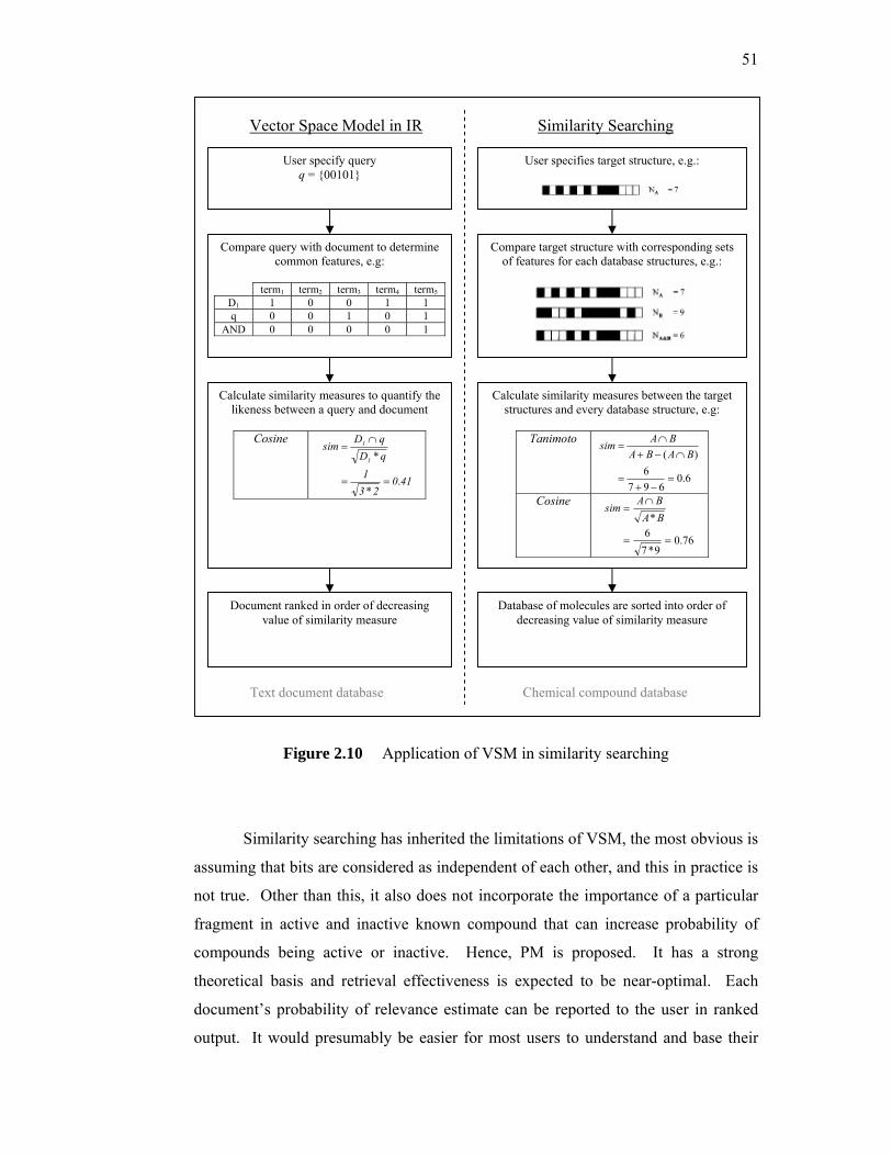
51
Figure 2.10 Application of VSM in similarity searching
Similarity searching has inherited the limitations of VSM, the most obvious is
assuming that bits are considered as independent of each other, and this in practice is
not true. Other than this, it also does not incorporate the importance of a particular
fragment in active and inactive known compound that can increase probability of
compounds being active or inactive. Hence, PM is proposed. It has a strong
theoretical basis and retrieval effectiveness is expected to be near-optimal. Each
document’s probability of relevance estimate can be reported to the user in ranked
output. It would presumably be easier for most users to understand and base their
User specify query q = {00101}
Compare query with document to determine common features, e.g:
term1 term2 term3 term4 term5
D1 1 0 0 1 1 q 0 0 1 0 1
AND 0 0 0 0 1
Document ranked in order of decreasing value of similarity measure
User specifies target structure, e.g.:
Compare target structure with corresponding sets of features for each database structures, e.g.:
Calculate similarity measures between the target structures and every database structure, e.g:
Tanimoto
6.0697
6)(
=−+
=
∩−+∩
=BABA
BAsim
Cosine
76.09*7
6*
==
∩=
BABAsim
Database of molecules are sorted into order of decreasing value of similarity measure
Vector Space Model in IR Similarity Searching
Chemical compound database Text document database
Calculate similarity measures to quantify the likeness between a query and document
Cosine
41023
1qDqDsim
1
1
.*
*
==
∩=

52
stopping behaviour upon a probability of relevance than a cosine similarity value.
The PM approach has yet to be applied in the compound retrieval system. Hence, to
close the knowledge gap, these alternatives of information retrieval in compound
similarity searching, need to be taken up, and determine whether PM is better in
terms of retrieving structures from chemical databases.
2.8 Summary
In this chapter, we have discussed important fundamentals of IR and
chemical retrieval system. Just as a document is relevant or not to a particular user’s
query, so is a molecule active or inactive, in some particular biological test.
Similarity in text and chemical database particularly in representation of records, has
allow application of algorithms for processing textual databases to processing
chemical structure. For this project, it is in terms of applying PM in similarity
searching, mainly the BIR model and BD model. Other than that, we also discussed
about the important elements in calculating similarity measures. There are molecular
representation and similarity coefficient to quantify the similarity between the
representations of two molecules. In the next chapter, details the real
implementation of the proposed approach in the chemical database environment.
Project methodology covers the experimental designs as well as data and equipment
used in this project.

CHAPTER 3
METHODOLOGY
In the previous chapter, we have discussed on the chemical compound
similarity searching as well as the IR models in detail. The chapter also covers how
both of these fields are related with each other. As the objective of this project is to
apply the Probability Model in chemical compound similarity searching, hence there
is a need to investigate whether the proposed approach yields better performance of
screening chemical compounds compared to the existing method. This chapter
discusses about the steps taken to carry out this research. It mainly focuses on the
computational experiment designs (Figure 3.1) where it details about the data set,
structural descriptors and similarity searching methods used. Evaluation is also done
to analyse the performance of each of the similarity searching methods.
Figure 3.1 Outline of Chapter 3
Computational Experiment Design
Test Data Set
Structural Descriptors
Similarity Searching Method
Performance Evaluation
VSM PM (BIR &
BD)
GH Score
Initial Enhance-
ment
Top 5% NCI AIDS Database
BCI bit string

54
3.1 Computational Experiment Design
The basis of this study comes from the virtual screening environment itself.
In a similarity search of a corporate database, a known bioactive compound is used
as a target structure to prioritise molecules for biological screening. An effective
similarity method will give a high percentage of actives among those compounds
ranked highest in terms of structural similarity with that target. As the similarity
values decreases, the percentage of actives covered will become gradually less. This
is because more and more dissimilar molecules are used, with no actives covered
when the compounds and the active target have no structural similarity between
them.
Figure 3.2 depicts the work flow of the computational experiment of this
project. Using the NCI AIDS dataset as the test data set, all chemical structures are
firstly represented using the BCI bit string. Then, a series of simulated similarity
searching studies is conducted to compare the effectiveness of different similarity
methods. In the data set, each active compound acts as a probe to search the
remainder of the data set. Compounds are then ranked according to the calculated
similarity values, from most to least similar. Lastly, the ranked list is analyzed to
determine which method is better. In doing so, we need to consider an important
criterion, which is: how good are the methods in separating active and inactive
structures? (Sheridan and Kearsley, 2002). It is not the absolute similarity value that
determines which method is better because it is generally not comparable between
methods. Hence, three approaches in evaluating the performance of the search
methods are taken up, mainly the GH score, initial enhancement and the number of
actives at top 5% of ranked list. Details of this approaches is explained in the
following sections.

55
Figure 3.2 Workflow of the simulated similarity searching.
3.2 Test Data Sets
Evaluating the performance of different similarity measures requires an ideal
test data set that satisfies the following requirement (Chen and Reynolds, 2002) that
is it should sample the chemical regions it covers as thoroughly as possible so that it
can really test the capability of a similarity measure to differentiate between active
and inactive structure.
The experiment here uses the National Cancer Institute (NCI) AIDS Database
(National Cancer Institute, 1999) as the test data set to satisfy this requirement. It
represents a large data set composed of both active and inactive compounds against a
specific therapeutic target and provides a thorough sampling of a particular region in
chemical space. This public database contains 5772 compounds, including 247
confirmed active (CA), 802 confirmed moderately active (CM) and 4723 confirmed
inactive (CI). In this data set, both the CA and CM are treated equally as actives and
the CI as inactive. The following shows the format of the input file for the dataset as
well as some sample data:
Query molecule posted
Perform similarity searching
Convert database to bit strings
Display chemical structures retrieved
Analyse performance

56
{compound name} {A list of bits set to 1 in the bit string} {Separator} {Total bits set to 1} aids99_CA_STR1 1 3 6 8 19 77 80 81 99 103 . . . 0 117 aids99_CM_STR10 1 6 8 39 46 86 89 149 242 298 . . . 0 53 aids99_CI_STR100 1 2 3 6 8 14 16 38 40 45 . . . 0 72
Figure 3.3 File format of data set with sample data (aids99_5772.bci1052.txt)
The above data set file can also be used to generate an inverted file. Inverted
file consist of a list of molecule IDs containing fragments. It is mostly used in this
work, to determine total number of structures that contains a particular bit bi, where i
refers to the location of the bit b in the bit string. This is also known as the notation
ni, mostly used in the BIR and BD model. The following shows the format of the
inverted file created based on the dataset, together with some sample data:
{Bit number} {A list of structures containing bit bi} {Separator} {Total structures
containing bit bi } 1 1 3 4 5 6 7 8 9 10 11 12 13 14 15 16 17. . . 0 4663 2 2 4 5 7 8 9 17 24 28 34 38 39 40 49 50 . . . 0 2986 3 1 3 5 7 8 9 10 11 12 13 14 15 16 17 18. . . 0 3487
Figure 3.4 File format of inverted file with sample data (inverted.txt)
3.3 Structural Descriptors
A chemical structure in this work is represented using BCI (Barnard
Chemical Information Ltd.) bit string. A molecule is divided into fragments of
specific functional groups or substructures. The fragments are recorded in a
predefined fragment dictionary that specifies the corresponding bit positions of the
fragments in the bit string. Bits represent the absence or presence of fragments either
individually or as a group. The following figure shows an example of a simple bit
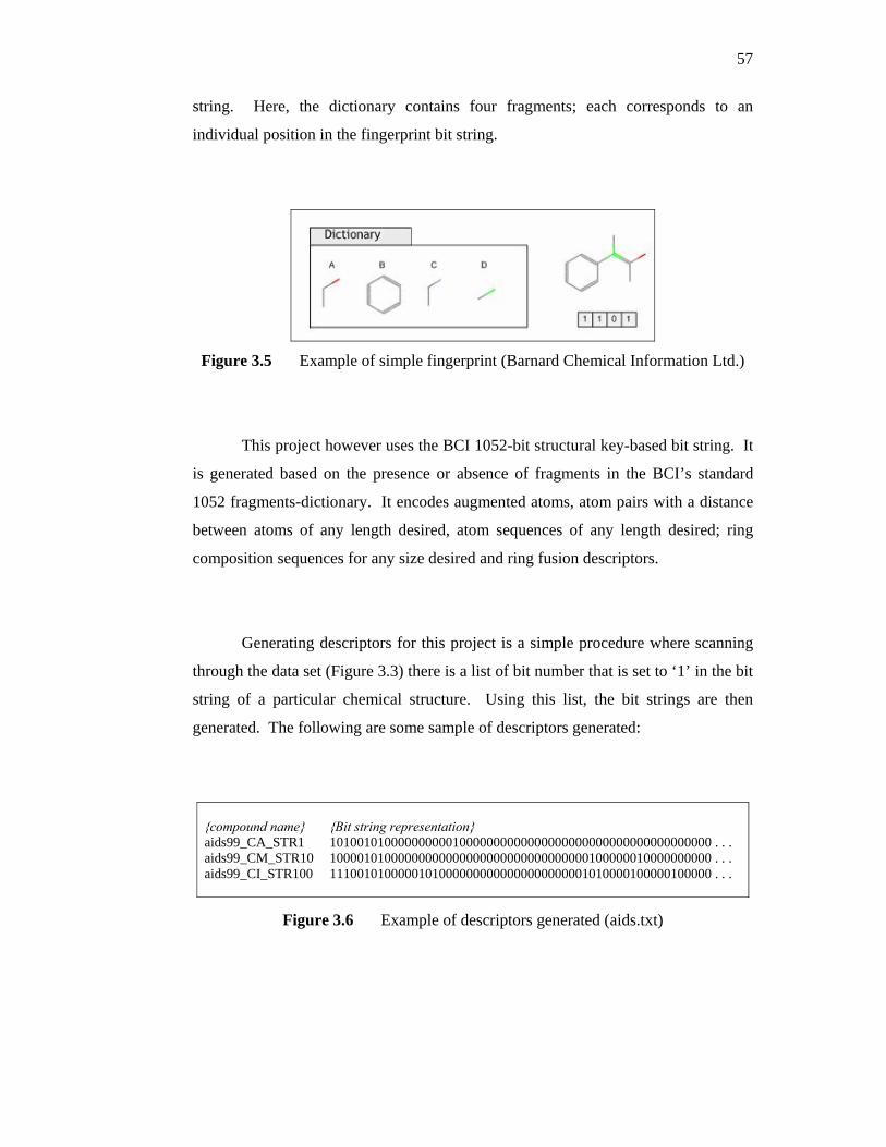
57
string. Here, the dictionary contains four fragments; each corresponds to an
individual position in the fingerprint bit string.
Figure 3.5 Example of simple fingerprint (Barnard Chemical Information Ltd.)
This project however uses the BCI 1052-bit structural key-based bit string. It
is generated based on the presence or absence of fragments in the BCI’s standard
1052 fragments-dictionary. It encodes augmented atoms, atom pairs with a distance
between atoms of any length desired, atom sequences of any length desired; ring
composition sequences for any size desired and ring fusion descriptors.
Generating descriptors for this project is a simple procedure where scanning
through the data set (Figure 3.3) there is a list of bit number that is set to ‘1’ in the bit
string of a particular chemical structure. Using this list, the bit strings are then
generated. The following are some sample of descriptors generated:
{compound name} {Bit string representation} aids99_CA_STR1 10100101000000000010000000000000000000000000000000000000 . . . aids99_CM_STR10 10000101000000000000000000000000000000100000010000000000 . . . aids99_CI_STR100 11100101000001010000000000000000000001010000100000100000 . . .
Figure 3.6 Example of descriptors generated (aids.txt)

58
3.4 Experiment 1: Comparing the Effectiveness of Similarity Searching
Methods
This project deals with three similarity searching methods. The first is the
existing approach in similarity searching which is based on the VSM. Here, the
Tanimoto coefficient is used as the similarity measure. The second approach
involves applying the PM in similarity searching. There are two models that are used
here namely the Binary Independence Retrieval (BIR) and Binary Dependence (BD)
Model. According to Losee (1994), BD model has actually improved the
performance of retrieval system compared to those applying independence
assumptions of terms. Even though, it is theoretically stronger than the BIR model,
its performance is yet to be proven in the chemical compound database.
3.4.1 Vector Space Model
As explained in the literature review, the industry standard similarity
searching process for bit-string based representation consists of the following steps.
First, specify the specification of an entire target structure. Then, compare the target
structure with corresponding set of features for each database structure. Each
comparison enables the calculation of a measure of similarity. In order to do so, the
Tanimoto coefficient is used. Hence, the measure of similarity between a compound
structure A and B is defined as follows:
cbacBAsim−+
=),(
a is the number of unique fragments in compound A,
b is the number of unique fragments in compound B,
where
c is the number of unique fragments shared by compounds A and B.

59
It is chosen because it is the standard for measuring the binary structural
similarity of compounds and it has one of the best overall performances compared to
other coefficients (Salim, 2002). Finally, the retrieval system ranks structures based
on their similarity to the target structure. They are sorted into order of decreasing
value of similarity measure. Figure 3.7 details the algorithm of this similarity
method.
Figure 3.7 Algorithm of existing similarity searching method
3.4.2 Binary Independence Retrieval Model
A chemical compound structure is represented using the binary indexing
concept. To apply BIR model, bits of a chemical structure S are map onto disjoint
concept by forming conjuncts of all bit b, in which each bit occurs either positively
or negated, that is:
n1nb1bS αα ∩∩= ... with =i
ibα ⎪⎩
⎪⎨⎧ =
=
1 if ib
0 if ib i
i
α
α
1. Post active structure as query 2. For every structure in database
2.1. common = 0 2.2. For all structure screen, i
2.2.1. if query.screen[i] = ‘1’ and structure.screen[i] = ‘1’ common = common +1
2.3. Calculate similarity 2.3.1. a = total bits set to 1 for query 2.3.2. b = total bits set to 1 for structure 2.3.3. c = common 2.3.4. tanimoto = c / (a +b-c)
3. Rank structures in decreasing order of Tanimoto scores

60
bi refers to bit b at location i on the bit string, where
αi acts as binary selector. If is αi = 1, then the bit occurs in the structure,
otherwise it is 0 and assumed negated.
In order to estimate the ranking score of a particular structure against the
target structure or query, the optimal similarity function is the ratio of probability of
active structures (P (A|S)) to probability of inactive structures (P (NA|S)). This is
also referred to as the Retrieval Status Value (RSV). Based on the Bayes theorem,
the similarity function becomes the following:
)|()()|()(
)|()|(
NASPNAPASPAP
SNAPSAP
⋅⋅
= (3.1)
P(S|A) is the probability of an active structure,
P(S|NA) is the probability of an inactive structure,
P(A) is the probability of actives,
where
P(NA) is the probability of inactives.
However, we need to associate the relevance of a structure to an explicit
feature. Two variables are used which are pi (probability that bit bi appearing in an
active structure) and qi (probability that bit bi appearing in an inactive structure).
Hence, we get the following expression of P (S|A) and P (S|NA):
ii
ii
1in1i i
1in1i i
q1qNASP
p1pASPαα
αα
−
=
−
=
−=
−=
∏∏
)()()|(
)()()|(
..
.. (3.2)
Then, by substituting (3.2) in (3.1) and taking logs of the ranking function, it
will turn into a linear discriminate function as stated below:

61
∑
∑
∑
∩∈
=
=
=
+=
+⎟⎟⎠
⎞⎜⎜⎝
⎛−−
+⎟⎟⎠
⎞⎜⎜⎝
⎛−−
=
qSbii
n
1iii
i
i
ii
iin
1ii
i
c
Cc
NAPAP
q1p1
p1qq1p
SNAPSAP
α
α
α)(
)(loglog)()(log
)|()|(
where ci indicates the capability of bit bi to discriminate active from inactive
structure. It is the only term considered here as it is associated with the binary
selector αi. Constant C is ignored because it is the same for all structures, hence
having no effect on the expression. In addition, it is assumed that pi = qi for all terms
not included in the query formulation (Fuhr, 1992). This restricts the evaluation of
the sum to query bits and thus producing the above expression.
In a chemical compound database, the activity and inactivity of a particular
structure is already determined. Hence we can estimate the probabilities P (S|A) and
P (S|NA) based on the contingency table in Table 3.1:
Table 3.1: Contingency table of relevance judgement (van Rijsbergen, 1979)
Active Inactive
αi = 1 a n-a n
αi = 0 A-a N-n-A+a N-n
A N-A N
Here, N is the total number of structures in the database, n refers to the total
number of structures which contain bit bi, A is the total the total number of active
structures, and a refers to the total number of active structures containing bit bi.
From this table, the following is estimated:
a) pi = ai / A
b) qi = (ni - ai) / (N - A)

62
Hence, the ci can be rewritten as:
))(()(log
aAananANaci −−
+−−=
However, the formulas of pi and qi may pose problems for small values of A
and ai. To avoid these problems, an adjustment factor is added which yields:
a) pi = (ai + 0.5) / (A + 1)
b) qi = (ni - ai + 0.5) / (N – A + 1)
Figure 3.8 summarizes the algorithm of this similarity searching method.
Figure 3.8 BIR model algorithm
1. Post active structure as query 2. N = Total number of structures in database 3. A = Total number of active structures in database 4. Determine ai
4.1. For each screen i 4.1.1. ai = Total number of structures which is a subset of A containing bit bi
5. For every structure in the database 5.1. Calculate similarity
5.1.1. RSV = 0.0 5.1.2. For every common bit shared by both query and structure
5.1.2.1. pi = (ai + 0.5) / (A + 1) 5.1.2.2. qi = (ni - ai + 0.5) / (N – A + 1) 5.1.2.3. RSV = RSV + log10 (pi / (1- pi )) + log10 ( (1- qi ) / qi)
6. Rank structures in decreasing order of their RSV

63
3.4.3 Binary Dependence Model
Bit dependencies refer to the presence or absence of a bit which provides
information about the probability of presence or absence of another bit. Assume
vector structure, S = {b1, b2 . . . bn} are binary values. It is arbitrarily complex to
capture all dependence data as we need to condition each variable in turn on a
steadily increasing set of other variable. Hence, to estimate probability of a structure
(P(S)) this model captures only the significant pairwise dependence information.
Thus P(S) is the probability of a bit i solely dependent on some preceding bit bj(i):
ij(i)0 n
1i ijbibPSP ≤≤∏=
= ))(|()( (3.4)
A probability distribution that can be represented as in the above expression
is called a probability distribution of first-order tree dependence (Chow and Liu,
1968). Take for example the following dependence tree:
Figure 3.9 A dependence tree
From equation (3.4), the probability of a structure can be written as
P(b1)P(b2|b1) P(b3|b1) P(b4|b2) P(b5|b2), or the following product expansion:
P(b1)P(b2|bj(2)) P(b3|bj(3))… P(bn|bj(n))
where the function j(i) exhibits the limited dependence of one bit on preceding bits.
b1
b4 b5
b3b2

64
There are many possible dependence tree that can be generated to find the
best ordering and mapping of j(i). Chow and Liu (1968) suggest constructing a
Maximum Spanning Tree (MST) using the Expected Mutual Information Measure
(EMIM). EMIM is a measure of a variable containing the information about another
variable. Hence, it requires the counting of co-occurrences of bits in a structure, and
thus used to measure the dependence between a pair of bits.
Let G(V,E) be a connected graph, where V is the set of nodes and E is the set
of edges. Assign to each edge (i, j(i)) a weight w(i, j(i)) obtained from calculating the
EMIM value of the pair of variable. An MST is a tree that includes every node and
has maximal total weight. It simply maximizes the sum:
∑ji
iji bbI,
)( ),(
where I(bi, bj(i)) represents the expected mutual information between bit bi and bj(i),
∑=)(, )(
)()()( )()(
),(log),(),(
iji bb iji
ijiijiiji bPbP
bbPbbPbbI
The contingency table below further simplify the calculation of EMIM in to
the following:
))(()(log)(
))(()(log)(
))(()(log)(
))(()(log)(),( )( 86
4485
3376
2275
11bbI iji +++=
Table 3.2: Contingency table of maximum likelihood estimates
bi = 1 bi = 0
bj(i) = 1 (1) (2) (7)
bj(i) = 0 (3) (4) (8)
(5) (6) (9)
Hence, the first step in this model is to generate the MST to identify the most
important pairwise dependencies. Each given chemical structure collection will

65
construct an MST based on all bits included in the collection. There are many
algorithms in generating an MST from pairwise association measures. The most
efficient is by Whitney (1972). It is based on the Dijkstra technique where a
maximum spanning tree is grown by successively adjoining the farthest remaining
node to a partially formed tree until all node of the graph are included in the tree
(Figure 3.10).
Figure 3.10 The Dijkstra algorithm
Figure 3.11 further summarises the algorithm for constructing the dependence
tree in this work. At each iterative step, the unsolved nodes are stored in array
not_in_tree. The node of the partially completed tree with the largest value of
EMIM to node not_in_tree[i] is stored in the array farthest_existing_node[i] and the
length or weight of edge from not_in_tree[i] to farthest_existing_node[i] is stored in
biggest_edges[i]. Hence, the node not yet in the tree which is farthest to a node of
the tree may be found by searching for the maximal element of array biggest_edge.
It is then added to the tree and removed from array not_in_tree. For each remaining
in array not_in_tree, the distance from farthest node of the tree (stored in
biggest_edge) is compared to the distance from the new node of the tree. Then the
array biggest_edge and farthest_existing_node is updated if the new distance is
farther. This process is repeated until all nodes are in the tree.
1. To initialise: 1.1. Start with graph G0 = (V0, E0) consisting of a single solved
node. 1.2. The arc set is empty.
2. Find all unsolved nodes that are directly connected by a single arc to any solved node (i, j(i)). For each unsolved node, calculate the weight w(i, j(i)) based on the EMIM value .
3. Choose the largest value of EMIM and add the corresponding unsolved node to the solved set. Also add the corresponding edge to the arc set.
4. If the newly solved node is not the destination node then repeat the process again.

66
Figure 3.11 The MST construction algorithm
Next, the dependence tree is then used to expand the query by taking the
original query bits and adding all bits that are immediately adjacent in the MST. The
pairwise term dependencies obtained for all bit pairs bi and bj in the expanded query
such that each pair (bi, bj) is represented by an edge in the spanning tree.
1. Calculate EMIM 1.1. For (i = 0; i< MAXSCREENS, i++)
1.1.1. For (j = i ; j< MAXSCREENS, j++) 1.1.1.1. Calculate EMIM for bit i and bit j and stored in array
DM[i][j] 1.1.1.2. DM[i][j] = DM[j][i]
2. Initialise the following: 2.1. num_nodes_outside = MAXSCREENS-1 2.2. new_node = MAXSCREENS-1 2.3. num_of_edges = 0 2.4. for i = 0 to i < num_nodes_outside
2.4.1. not_in_tree[i] = i 2.4.2. biggest_edges[i] = DM[i][new_node] 2.4.3. farthest_existing_node[i] = new_node
3. Update labels of nodes not yet in tree 3.1. for i = 0 to i < num_nodes_outside
3.1.1. outside node = not_in_tree[i] 3.1.2. edge weight = DM[outside node][new_node] 3.1.3. if (biggest_edges[i] < edge weight)
biggest_edges[i] = edge weight farthest_existing_node[i] = new_node
4. Find node outside tree farthest from tree 4.1. best edge = biggest_edges[0] 4.2. for i = 0 to i < num_nodes_outside
4.2.1. if (biggest_edges[i] > best edge) best edge = biggest_edges[i] best node = i
4.3. MST[num_of_edges][0] = not_in_tree[best node] 4.4. MST[num_of_edges][1] = farthest_existing_node[best node] 4.5. new_node = not_in_tree[best node] 4.6. num_of_edges = num_of_edges + 1
5. Delete new tree node from array not_in_tree 5.1. biggest_edges[best node] = biggest_edges[num_nodes_outside - 1] 5.2. not_in_tree[best node] = not_in_tree[num_nodes_outside - 1] 5.3. farthest_existing_node[best node] = closet_existing_node
[num_nodes_outside - 1] 5.4. num_nodes_outside = num_nodes_outside -1
6. Repeat Step 3 to 5 until num_nodes_outside = 0

67
The following explains the similarity function or RSV of this model. As
mentioned in section 3.4.2, the similarity function is as stated in expression (3.1).
Based also the discussion in this section, we have found that only the term P(S|A)
and P(S|NA) are considered. The rest remains as a constant and does not include in
the calculation of RSV. Hence obtaining the expression:
NA)|P(S log - A)|P(S SNAP
SAP log)|(
)|(= (3.5)
For each structure S, the factors P(S|A) and P(S|NA) are computed using the
following expression:
Cn
2i iqijiq1iq1ijiq
ijbibiq1
ijiq1
ijbn
1i iq1iq
ibNASP
Cn
2i ipijip1ip1ijip
ijbibip1
ijip1
ijbn
1i ip1ip
ibASP
+∑= −
−+
−
−+∑
= −=
+∑= −
−+
−
−+∑
= −=
]))(|(
)()(|log)()(|log)([]log[)|(log
]))(|(
)()(|log)(
)(|log)([]log[)|(log
(3.6)
bi refers to bit b at location i,
bj(i) refers to bit b at location j(i) where bit bj(i) is the preceding bit of bit bi,
pi|j(i) is the probability of both bit bi and bit bj(i) appearing in active structures,
pi is the probability of both bit bi appearing in active structures,
qi|j(i) is the probability of both bit bi and bit bj(i) appearing in inactive structures,
where
qi is the probability of both bit bi appearing in inactive structures,
Then, by substituting (3.6) in (3.5), and taking into account that P(bi =1 | bj(i)
= 1, A) = P (bi = 1, bj(i) = 1, A) / P( bj(i) = 1 | A), hence it further transform the
expression into the following:
])()(
log)()(
log)()(
[log
])(
log)(
[log])()(
log[)|()|(
)()(
)()(
)(|)(|
)(|)(|)(
)(
)(|)(
)(
)(|)()(
ijij
ijij
ii
iin
2i ijiiji
ijiijiiji
n
2i iij
ijiij
iij
ijiijij
n
1i ii
iii
p1qq1p
p1qq1p
p1qq1p
bb
q1qqq
p1ppp
bp1qq1p
bSNAPSAP
−
−−
−−
−−
−+
−
−−
−
−+
−−
=
∑
∑∑
−
==
(3.7)

68
Relevance information is available in the database, this model computes the
probability of P(S|A) and P(S|NA) using the same contingency table as the BIR
model (Table 3.1) and thus producing the following assumption. The adjustment
factor is also taken in consideration to avoid problem occurring from small value of
A and ai.
a) pi = (ai + 0.5) / (A + 1)
b) qi = (ni - ai + 0.5) / (N – A + 1)
c) pj(i) = (V j(i) + 0.5) / (A + 1)
d) q j(i) = (n j(i) - a j(i) + 0.5) / (N – A + 1)
e) pi|j(i) = (a i|j(i) + 0.5) / (A + 1)
f) q i|j(i) = (n i|j(i) - a i|j(i) + 0.5) / (N – A + 1)
where N is the number of structures in database
ni refers to the frequency of structure containing bit bi
nj(i) refers the frequency of structure containing bit bj(i)
ni|j(i) refers to the frequency of structure containing both bit
bi and bit bj(i)
A is the total number of active structures
a refers to the total number of active structures
containing a particular bit b
Figure 3.12 summarizes the algorithm of this similarity searching method.
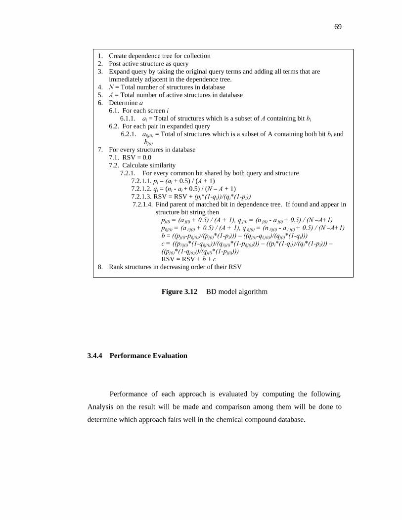
69
Figure 3.12 BD model algorithm
3.4.4 Performance Evaluation
Performance of each approach is evaluated by computing the following.
Analysis on the result will be made and comparison among them will be done to
determine which approach fairs well in the chemical compound database.
1. Create dependence tree for collection 2. Post active structure as query 3. Expand query by taking the original query terms and adding all terms that are
immediately adjacent in the dependence tree. 4. N = Total number of structures in database 5. A = Total number of active structures in database 6. Determine a
6.1. For each screen i 6.1.1. ai = Total of structures which is a subset of A containing bit bi
6.2. For each pair in expanded query 6.2.1. ai|j(i) = Total of structures which is a subset of A containing both bit bi and
bj(i) 7. For every structures in database
7.1. RSV = 0.0 7.2. Calculate similarity
7.2.1. For every common bit shared by both query and structure 7.2.1.1. pi = (ai + 0.5) / (A + 1) 7.2.1.2. qi = (ni - ai + 0.5) / (N – A + 1) 7.2.1.3. RSV = RSV + (pi*(1-qi))/(qi*(1-pi)) 7.2.1.4. Find parent of matched bit in dependence tree. If found and appear in
structure bit string then pj(i) = (a j(i) + 0.5) / (A + 1), q j(i) = (n j(i) - a j(i) + 0.5) / (N –A+1) pi|j(i) = (a i|j(i) + 0.5) / (A + 1), q i|j(i) = (n i|j(i) - a i|j(i) + 0.5) / (N –A+1) b = ((pj(i)-pi|j(i))/(pj(i)*(1-pi))) – ((qj(i)-qi|j(i))/(qj(i)*(1-qi))) c = ((pi|j(i)*(1-qi|j(i)))/(qi|j(i)*(1-pi|j(i)))) – ((pi*(1-qi))/(qi*(1-pi))) – ((pj(i)*(1-qj(i)))/(qj(i)*(1-pj(i)))) RSV = RSV + b + c
8. Rank structures in decreasing order of their RSV

70
a) GH Score (Güner, 1998)
The GH score gives an indication of how good the retrieved list is with
respect to a compromise between maximum yield and maximum percent
of actives retrieved. Consider the following:
D is the number of chemical structures in the database,
A is the number of actives structures in the database,
Ht is the number of structures in a retrieved list, and
Ha is the number of active structures in a retrieved list.
Figure 3.13 Schematic representation of the chemical database
space, actives and hit (retrieved compound) list (Güner, 1998).
The different metrics that can be used to evaluate the quality of a hit list
are given below:
The percent yield of actives or also referred to as proportion of
structures retrieved that are active (Precision).
100% ×=t
a
HHY
Percent ratio of the actives in the list or also referred to as
proportion of active structures that are retrieved (Recall).
100% ×=A
HA a
Number of actives not in the hit list:
False negative = A - Ha
Database
Actives
Hits
D
A
Ht Ha

71
Number of inactive structures in the hit list:
False positive = Ht - Ha
Thus, the GH score is actually the sum of yield and ratio of actives in the
hit list. It is then divided by two, as denoted below:
t
ta
a
t
a
AH2HAH
2A
HHH
2AYGH
)( +=
⎟⎠⎞
⎜⎝⎛+⎟⎟
⎠
⎞⎜⎜⎝
⎛
=+
=
b) Initial enhancement, which refers to a number of chemical structure
retrieved before half of the actives are found. The less the value, the
better the performance of the similarity searching system.
c) The number of actives at top 5% of the list. If there are quite a number of
active structures on the top 5% of this list, it denotes a good similarity
searching system.
3.5 Experiment 2: Comparing the Query Fusion Result of Similarity
Searching Methods
The purpose of this experiment is to investigate whether query fusion result
of the proposed probability models, is better than VSM. Data fusion is an approach
where data, evidence, or decisions coming from or based on multiple sources, about
the same set of objects are integrated to increase the quality of decision making
under uncertainty about the objects (Salim, 2002). The advantage of this approach is
that it can improve confidence in decisions with the use of complementary
information by inferring information that is outside of the capability of a single
sensor information.

72
IR systems apply data fusion in combining the following components:
multiple document representations, multiple queries and multiple retrieval
techniques. This section focuses on data fusion in combining multiple queries
(Belkin et. al., 1995). A number of studies have looked into the effect of capturing
multiple queries from a single searcher or multiple searchers given the same
specification of an information need, to get more evidence about relevance. Some
retrieval models were proposed that incorporates multiple representation of the
information need (Turtle and Croft, 1991; Rajashekar and Croft, 1995). Belkin et. al.
(1995) on the other hand, found that applying adaptive weighting schemes to query
combination gives better result than best individual system where progressive result
combination were taken into consideration.
In chemoinformatic, query combination is also being applied in combining
several molecules in a single query. Similarity searches using mixtures as queries
and/or database entries was found to give better or at least equal results to
experiments using single compounds as targets and database entries (Sheridan,
2000). Combined chemical target has also been used in an iterative similarity
searching using approach analogous to relevance feedback in the text retrieval area
(Singh et. al., 2001). Hence, based on this concept, this second experiment uses
combined chemical target in an iterative similarity searching to estimating
probability instead of obtaining from the entire collection.
The NCI AIDS dataset is divided equally to four sets, with 1443 structures in
each set. The NCI AIDS dataset organises compounds according to the following:
CA, CM and CI. Hence, this simplifies the division of the data sets with each set
having equal distribution of CA, CM and CI. The algorithm of this process is shown
in Figure 3.14 and the result of this division is shown in Table 3.3.
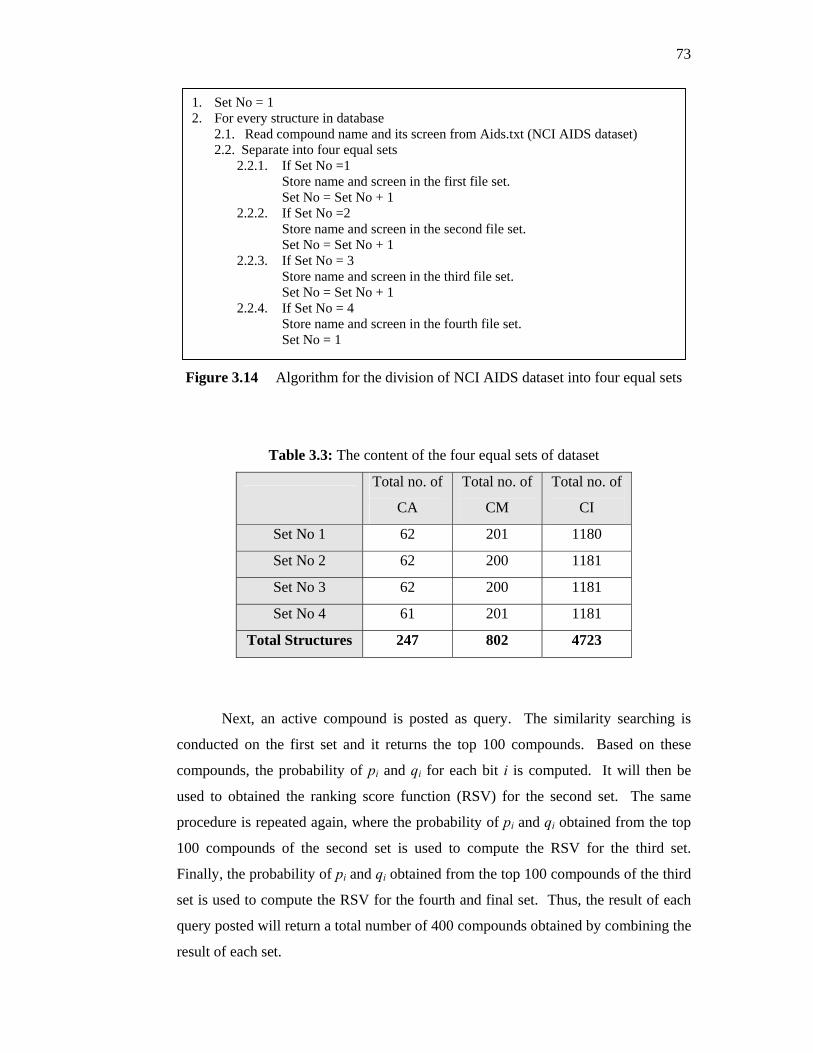
73
Figure 3.14 Algorithm for the division of NCI AIDS dataset into four equal sets
Table 3.3: The content of the four equal sets of dataset
Total no. of
CA
Total no. of
CM
Total no. of
CI
Set No 1 62 201 1180
Set No 2 62 200 1181
Set No 3 62 200 1181
Set No 4 61 201 1181
Total Structures 247 802 4723
Next, an active compound is posted as query. The similarity searching is
conducted on the first set and it returns the top 100 compounds. Based on these
compounds, the probability of pi and qi for each bit i is computed. It will then be
used to obtained the ranking score function (RSV) for the second set. The same
procedure is repeated again, where the probability of pi and qi obtained from the top
100 compounds of the second set is used to compute the RSV for the third set.
Finally, the probability of pi and qi obtained from the top 100 compounds of the third
set is used to compute the RSV for the fourth and final set. Thus, the result of each
query posted will return a total number of 400 compounds obtained by combining the
result of each set.
1. Set No = 1 2. For every structure in database
2.1. Read compound name and its screen from Aids.txt (NCI AIDS dataset) 2.2. Separate into four equal sets
2.2.1. If Set No =1 Store name and screen in the first file set. Set No = Set No + 1
2.2.2. If Set No =2 Store name and screen in the second file set. Set No = Set No + 1
2.2.3. If Set No = 3 Store name and screen in the third file set. Set No = Set No + 1
2.2.4. If Set No = 4 Store name and screen in the fourth file set. Set No = 1

74
3.5.1 Binary Independence Retrieval Model
Figure 3.15 summarizes the algorithm of this similarity searching method.
Figure 3.15 BIR model query combinational algorithm
3.5.2 Binary Dependence Model
Figure 3.16 summarizes the algorithm of this similarity searching method.
1. Separate datasets in 4 equally divided sets 2. Post active structure as query 3. N = Total number of structures in set 4. Conduct similarity searching on first set using the BIR model
4.1. A = Total number of active structures in first set 4.2. Determine ai
4.2.1. For each screen i 4.2.1.1. ai = Total number of structures which is a subset of A containing bit bi
4.3. Calculate similarity for every structure in the first set 4.3.1. RSV = 0.0 4.3.2. For every common bit shared by both query and structure
4.3.2.1. pi = (ai + 0.5) / (A + 1) 4.3.2.2. qi = (ni – ai + 0.5) / (N – A + 1) 4.3.2.3. RSV = RSV + log10 (pi / (1- pi )) + log10 ( (1- qi ) / qi)
4.4. Rank structures in decreasing order of their RSV 5. Retrieve top 100 compounds from the ranked list and obtain the following
5.1. V = Total number of active structures in the top 100 5.2. Determine Vi
5.2.1. For each screen i 5.2.1.1. Vi = Total number of structures which is a subset of V containing bit bi
5.3. Calculate similarity for every structure in the next set 5.3.1. RSV = 0.0 5.3.2. For every common bit shared by both query and structure
5.3.2.1. pi = (Vi + 0.5) / (V + 1) 5.3.2.2. qi = (ni – Vi + 0.5) / (N – V + 1) 5.3.2.3. RSV = RSV + log10 (pi / (1- pi )) + log10 ( (1- qi ) / qi)
5.4. Rank structures in decreasing order of their RSV 6. Repeat step 5 for set 3 and 4.

75
Figure 3.16 BD model combinational query result algorithm
1. Separate datasets in 4 equally divided sets 2. Post active structure as query 3. N = Total number of structures in set 4. Conduct similarity searching on first set using the BD model
4.1. Load dependence tree for set and expand query. 4.2. A = Total number of active structures in set 4.3. Determine V
4.3.1. For each screen i 4.3.1.1. ai = Total of structures which is a subset of A containing bit bi
4.3.2. For each pair in expanded query 4.3.2.1. ai|j(i) = Total of structures which is a subset of A containing both bit bi
and bj(i) 4.4. Calculate similarity for every structures in first set
4.4.1. RSV = 0.0 4.4.2. For every common bit shared by both query and structure
4.4.2.1. pi = (ai + 0.5) / (A + 1) 4.4.2.2. qi = (ni - ai + 0.5) / (N – A + 1) 4.4.2.3. RSV = RSV + (pi*(1-qi))/(qi*(1-pi)) 4.4.2.4. Find parent of matched bit in dependence tree. If found and appear in
structure bit string then pj(i) = (a j(i) + 0.5) / (A + 1), q j(i) = (n j(i) - a j(i) + 0.5) / (N –A+1) pi|j(i) = (a i|j(i) + 0.5) / (A + 1), q i|j(i) = (n i|j(i) - a i|j(i) + 0.5) / (N –A+1) b = ((pj(i)-pi|j(i))/(pj(i)*(1-pi))) – ((qj(i)-qi|j(i))/(qj(i)*(1-qi))) c = ((pi|j(i)*(1-qi|j(i)))/(qi|j(i)*(1-pi|j(i)))) – ((pi*(1-qi))/(qi*(1-pi))) – ((pj(i)*(1-qj(i)))/(qj(i)*(1-pj(i)))) RSV = RSV + b + c
4.4.3. Rank structures in decreasing order of their RSV 5. Retrieve top 100 compounds from the ranked list and obtain the following
5.1. V = Total number of active structures in the top 100 5.2. Determine Vi
5.2.1. For each screen i 5.2.1.1. Vi = Total number of structures which is a subset of V containing bit bi
5.2.2. For each pair in expanded query 5.2.2.1. Vi|j(i) = Total of structures which is a subset of V containing both bit bi
and bj(i) 5.3. Load dependence tree for the next set and expand query. 5.4. Calculate similarity for every structure in that set
5.4.1. RSV = 0.0 5.4.2. For every common bit shared by both query and structure
5.4.2.1. pi = (Vi + 0.5) / (V + 1) 5.4.2.2. qi = (ni - Vi + 0.5) / (N – V + 1) 5.4.2.3. RSV = RSV + (pi*(1-qi))/(qi*(1-pi)) 5.4.2.4. Find parent of matched bit in dependence tree. If found and appear in
structure bit string then pj(i) = (V j(i) + 0.5) / (V + 1), q j(i) = (n j(i) - V j(i) + 0.5) / (N –V+1) pi|j(i) = (V i|j(i) + 0.5) / (V + 1), q i|j(i) = (n i|j(i) - V i|j(i) + 0.5) / (N –V+1) b = ((pj(i)-pi|j(i))/(pj(i)*(1-pi))) – ((qj(i)-qi|j(i))/(qj(i)*(1-qi))) c = ((pi|j(i)*(1-qi|j(i)))/(qi|j(i)*(1-pi|j(i)))) – ((pi*(1-qi))/(qi*(1-pi))) – ((pj(i)*(1-qj(i)))/(qj(i)*(1-pj(i)))) RSV = RSV + b + c
5.4.3. Rank structures in decreasing order of their RSV 6. Repeat step 5 for set 3 and 4.

76
3.5.3 Performance Evaluation
Performance evaluation of each PM approach will be computed by
determining the average total number of actives at top 400 of the list. It is then
compared to the average total number of actives at top 400 of the VSM approach. A
good similarity searching system is denoted if there are quite a number of active
structures on the top 400 of the list.
3.6 Hardware and Software Requirements
In this section, hardware and software requirement of this project are stated.
The following is the list of hardware and software used to carry this project:
Table 3.4: Software Requirement
Software Details
1. Microsoft Visual C++ 6.0 All similarity searching programs will be developed using
the C++ language. Thus Visual C++ is used because it
provides a stable environment to develop a program and
an extensive help file.
2. Microsoft Office XP This software package will be used to prepare reports and
presentation file.
3. Microsoft Project 2000 This software is a popular project management tool. It is
used to generate Gantt charts for this projects planning.
4. Microsoft Windows XP As the operating system.

77
Table 3.5: Computer Specification
Component Specification
Processor: Intel Pentium IV 2.8 GHz
Memory: 512MB
Hard disk: 40GB
3.7 Discussion
This chapter gives details on how experiment is carried out to determine
whether the proposed approach have given us better performance result compared to
the existing similarity searching method. The aim of an effective retrieval system is
to respond to a query so as to retrieve most active chemical structure, while
retrieving very few inactive structures. A series of simulated similarity searching is
conducted for both existing and proposed approach. This experiment design has
been used on almost all research that involves determining the effectiveness of
similarity searching system. However, most experiment involves manipulating
between the main requirements of similarity searching which is the structural
descriptor and similarity coefficient, to determine which is superior (e.g. Chen and
Reynolds, 2002; Salim, 2002). Hence the same approach is also taken up in this
project.
We have chosen to base our comparison to VSM-based similarity searching
with 2D screens as its structural descriptor and Tanimoto coefficient as its similarity
measure. 2D screens particularly dictionary-based bit string are used here. In
Chapter 2, we have already discussed why this representation scheme is preferred
rather than the other alternative of 2D screen which is the very dense hashed
fingerprint.
78
For similarity measure, the Tanimoto coefficient is used. It is an association
coefficient where it is consider a common presence of attributes as evidence of
similarity. Association coefficient is also generally preferred to than the distance
coefficients. The difference between association and distance coefficient is that the
latter effectively consider a common absence of attributes as evidence of similarity,
whereas the former do not. Chen and Reynolds (2002) conducted experiments and
concluded that common presence of certain structural features is the primary factor
in determining similarity between two chemical structures. However, absence of
features may also be important in some cases but is at best considered secondary.
The proposed approaches for this work involve the PM (i.e. BIR and BD
model). It has already been discussed in detail in Chapter 2. However, now we are
no longer dealing with documents but chemical structures. Applying PM in chemical
database environment is very straight forward, particularly due to its similarity in
representing object. The following diagram summarises the framework in applying
PM in chemical databases:

79
Figure 3.17 Proposed framework
3.8 Summary
In the effort to improve chemical retrieval system, PM was proposed. Both
independent and dependent assumption of bits were considered, that is by applying
BIR and BD Model in chemical database environment. In this chapter, processing
steps have been discussed for each model. Overall, this project involves converting
database to bit strings, performing similarity searching when user posts a query and
displaying the result. Lastly, the performance of each approach is evaluated. Results
and analysis of the performance evaluation is presented and discussed in Chapter 4.
Query molecule
posted
Perform similarity searching
Similarity searching system
Binary Independence Retrieval Model
Binary Dependence Model
Convert database to bit
strings
Display chemical structures retrieved
Calculate ranking score
Ranked structure in decreasing order of score
Generate MST based on EMIM values calculated
Expand query
Calculate ranking score
Ranked structure in decreasing order of score

CHAPTER 4
RESULTS AND DISCUSSIONS
In Chapter 3, steps taken in conducting experiment in this project were
discussed. Thus, Chapter 4 presents the results of these experiments. This chapter is
very important as the outcomes will prove whether the proposed approaches are
more favourable in chemical database processing. The outline of this chapter is as
follows: As mentioned in previous chapters, the proposed PM-based similarity
searching system will be compared with the existing method. Hence, there are three
groups of result belonging to the VSM, BIR and BD model. There are 1049 active
compounds (i.e. both CM and CA) posted as target compound. The output of each
similarity searching system is a series of ranked list of structures, and stored in the
following output files: VSMResult.txt, BIRResult.txt and BDResult.txt. Format of
output file is as depicted in Figure 4.1. From each ranked list, we acquire the
performance evaluation for each method (Figure 4.2). Next, the average of 1049
(target compounds posted) performance evaluation is calculated, which consist of
the GH score, initial enhancement and total active structures at top 5% of the ranked
list, which is from the first experiment. The result of the second experiment is also
shown here which includes the average total active structures at top 400 of the
ranked list. Discussion in this chapter emphasizes on the critical analysis of the
results. This is done by comparing the results of all three approaches and stating
some observation based on it.

81
Figure 4.1 File format of output file.
Figure 4.2 Sample evaluation result for similarity searching system.
{Active molecule as target molecule} Query posted: 10100101000000000010000000000000000000000000000000000… {Structure ID} {Compound name} {Similarity / Ranking Score}
1 aids99_CA_STR1 1.0000 339 aids99_CM_STR193 0.9664 156 aids99_CA_STR282 0.8760
3 aids99_CA_STR102 0.8618 23 aids99_CA_STR125 0.8346
707 aids99_CM_STR58 0.8293 499 aids99_CM_STR36 0.8160 4097 aids99_CI_STR3895 0.7984 232 aids99_CA_STR8 0.7692 382 aids99_CM_STR238 0.7541
: : :
{Query No.} Query no. 1 {GH Score section consisting of values for recall, precision, GH score, false positive, false negative} GH Score: Recall Precisions GHScore False+ False- 12.3928 44.9827 28.6877 159 919 {Values at 5% of structure retrieved} 16.3012 29.5848 22.9430 407 878 {Values at 10% of structure retrieved} 20.4004 24.7113 22.5558 652 835 {Values at 15% of structure retrieved} 25.5481 23.2035 24.3758 887 781 {Values at 20% of structure retrieved} 30.1239 21.8837 26.0038 1128 733 {Values at 25% of structure retrieved} 34.7950 21.0739 27.9345 1367 684 {Values at 30% of structure retrieved} Initial enhancement: 2633 {No of structures retrieved before half of the active structures are found.} No of actives at top 5%: 130 {No of active structures retrieved at top 5% of the ranked list.} Query no. 2 GH Score: Recall Precisions GHScore False+ False- 5.4337 19.7232 12.5785 232 992 10.9628 19.8962 15.4295 463 934 15.2526 18.4757 16.8642 706 889 19.7331 17.9221 18.8276 948 842 26.2154 19.0443 22.6299 1169 774 30.9819 18.7644 24.8732 1407 724 Initial enhancement: 2926 No of actives at top 5%: 57 … Query no. 1049 GH Score: Recall Precisions GHScore False+ False- 7.6263 27.6817 17.6540 209 969 13.4414 24.3945 18.9179 437 908 19.1611 23.2102 21.1856 665 848 26.8827 24.4156 25.6492 873 767 32.9838 23.9612 28.4725 1098 703 39.0848 23.6721 31.3784 1322 639 Initial enhancement: 2399 No of actives at top 5%: 79

82
4.1 Results of VSM-based Similarity Searching
Table 4.1 shows the average result of VSM-based similarity searching in
terms of four evaluation merits discussed earlier. In the first experiment, readings of
GH scores are taken on each 5% interval of structure retrieved, which are 5%, 10%,
15% …30%. Readings stop at 30% of the structures retrieved. This means that the
final GH score value is obtained when 1732 compounds are retrieved. More than
this value is not considered because normally user will only look at most the top
1000 compounds. As seen in the table below, the GH score increases on each level.
This is expected as when we retrieved more structure we obtain more actives. While
computing GH scores, we can also acquire the values for false negative and false
positive on each level. This is to find out the number of active and inactive in the
ranked list, respectively. For initial enhancement we consider the number of
chemical structure retrieved before half of the actives are found. The VSM-based
similarity searching attains an average of 2705 compounds for this evaluation
criterion. Next, we can see that this approach returns an average of 73 active
compounds on top 5% of its ranked list. For the second experiment, the VSM-based
similarity searching obtains an average of 95 active structures at top 400 of its list.
Table 4.1: Summary of VSM Result
Experiment 1: 5% 10% 15% 20% 25% 30%Average GH Score 16.26 17.11 18.95 21.22 23.59 26.02Average False + 215 450 686 921 1157 1391Average False - 975 921 869 815 762 708
Average initial enhancement : 2705
Average number of actives at top 5% : 73
Experiment 2:
Average number of actives at top 400 : 95
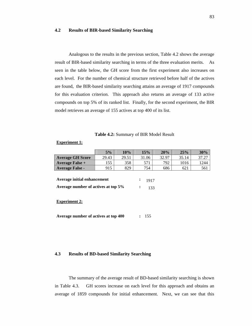
83
4.2 Results of BIR-based Similarity Searching
Analogous to the results in the previous section, Table 4.2 shows the average
result of BIR-based similarity searching in terms of the three evaluation merits. As
seen in the table below, the GH score from the first experiment also increases on
each level. For the number of chemical structure retrieved before half of the actives
are found, the BIR-based similarity searching attains an average of 1917 compounds
for this evaluation criterion. This approach also returns an average of 133 active
compounds on top 5% of its ranked list. Finally, for the second experiment, the BIR
model retrieves an average of 155 actives at top 400 of its list.
Table 4.2: Summary of BIR Model Result
Experiment 1: 5% 10% 15% 20% 25% 30%Average GH Score 29.43 29.51 31.06 32.97 35.14 37.27Average False + 155 358 571 792 1016 1244Average False - 915 829 754 686 621 561
Average initial enhancement : 1917Average number of actives at top 5% : 133
Experiment 2:
Average number of actives at top 400 : 155
4.3 Results of BD-based Similarity Searching
The summary of the average result of BD-based similarity searching is shown
in Table 4.3. GH scores increase on each level for this approach and obtains an
average of 1859 compounds for initial enhancement. Next, we can see that this

84
approach returns an average of 141 active compounds on top 5% of its ranked list.
For the second experiment, the BD model obtains an average of 160 actives at top
400 of its list.
Table 4.3: Summary of BD Model Result
Experiment 1: 5% 10% 15% 20% 25% 30%Average GH Score 31.20 30.86 32.26 34.19 36.18 38.16Average False + 147 348 559 779 1004 1233Average False - 907 819 742 673 609 550
Average initial enhancement : 1859Average number of actives at top 5% : 141
Experiment 2:
Average number of actives at top 400 : 160
4.4 Discussion
In this section, two issues need to be determined. The first being whether the
PM-based similarity searching overcomes the existing approach. If so, which of the
probability models proposed is more superior in the chemical database environment.
Hence, in each performance criterion, these two issues are taken into consideration.
The following is the comparison made for all three approaches of similarity
searching involved in this work, with respect to the performance criterion below:
a) Experiment 1: Comparing the Effectiveness of Similarity Searching
Methods

85
GH Score
In the following figure, GH score values at each 5% level of the
structure retrieved are plotted for all the similarity searching method.
As seen in the graph, we can conclude that both PM approaches
outperform the existing system.
As GH score gives quantitative measure of the ranked list quality, we
can confirm the PM approaches is substantially more selective than
the others without compromising present of actives too much. The
graph also shows that the BD model’s GH score performance exceed
the BIR model but only slightly.
GH Score
0,00
5,00
10,00
15,00
20,00
25,00
30,00
35,00
40,00
45,00
5% 10% 15% 20% 25% 30%
% structures retrieved
%G
H
BIM VSM BDM Figure 4.3 GH score analysis for VSM, BIR and BD model.
False Positive and False Negative
Figure 4.4 shows the number of inactive structures in the ranked list,
whereas Figure 4.5 shows the number of actives not in the ranked list.
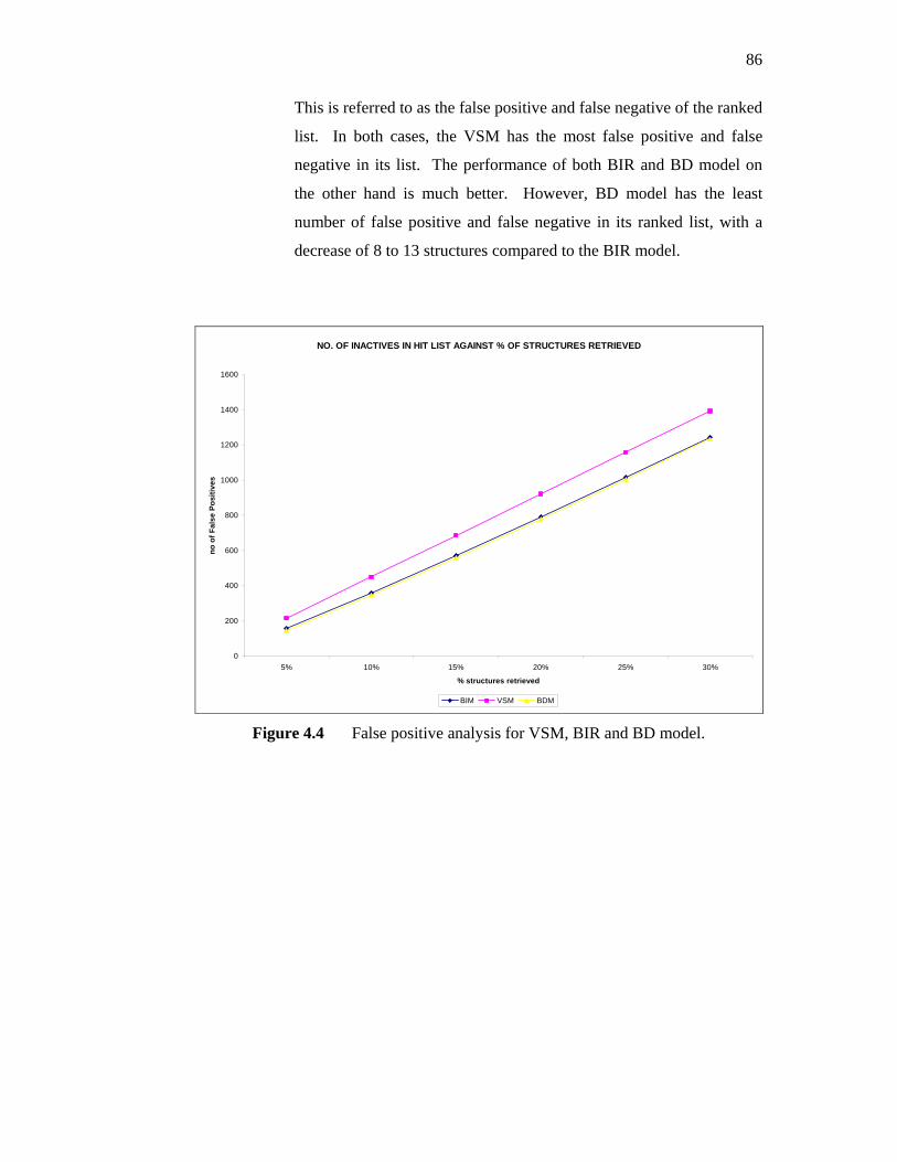
86
This is referred to as the false positive and false negative of the ranked
list. In both cases, the VSM has the most false positive and false
negative in its list. The performance of both BIR and BD model on
the other hand is much better. However, BD model has the least
number of false positive and false negative in its ranked list, with a
decrease of 8 to 13 structures compared to the BIR model.
NO. OF INACTIVES IN HIT LIST AGAINST % OF STRUCTURES RETRIEVED
0
200
400
600
800
1000
1200
1400
1600
5% 10% 15% 20% 25% 30%
% structures retrieved
no o
f Fal
se P
ositi
ves
BIM VSM BDM Figure 4.4 False positive analysis for VSM, BIR and BD model.

87
NO OF ACTIVES NOT IN HIT LIST AGAINST % OF STRUCTURES RETRIEVED
0
200
400
600
800
1000
1200
5% 10% 15% 20% 25% 30%
% structures retrieved
no o
f Fal
se N
egat
ive
BIM VSM BDM Figure 4.5 False negative analysis for VSM, BIR and BD model.
Average Initial Enhancement
As discussed in Chapter 3, initial enhancement refers to the number of
chemical structure retrieved before half of the actives are found.
Hence, the performances of similarity searching methods are
comparable, with the superior system having less value of initial
enhancement. The figure below shows us that again the VSM has the
highest value of initial enhancement. It retrieves approximately 800
more structures compared to the PM approaches.
Here again we can see that BD model is more superior in term of
average initial enhancement. BIR model retrieves 58 more structures
before half of the actives are found compared to the BD model.
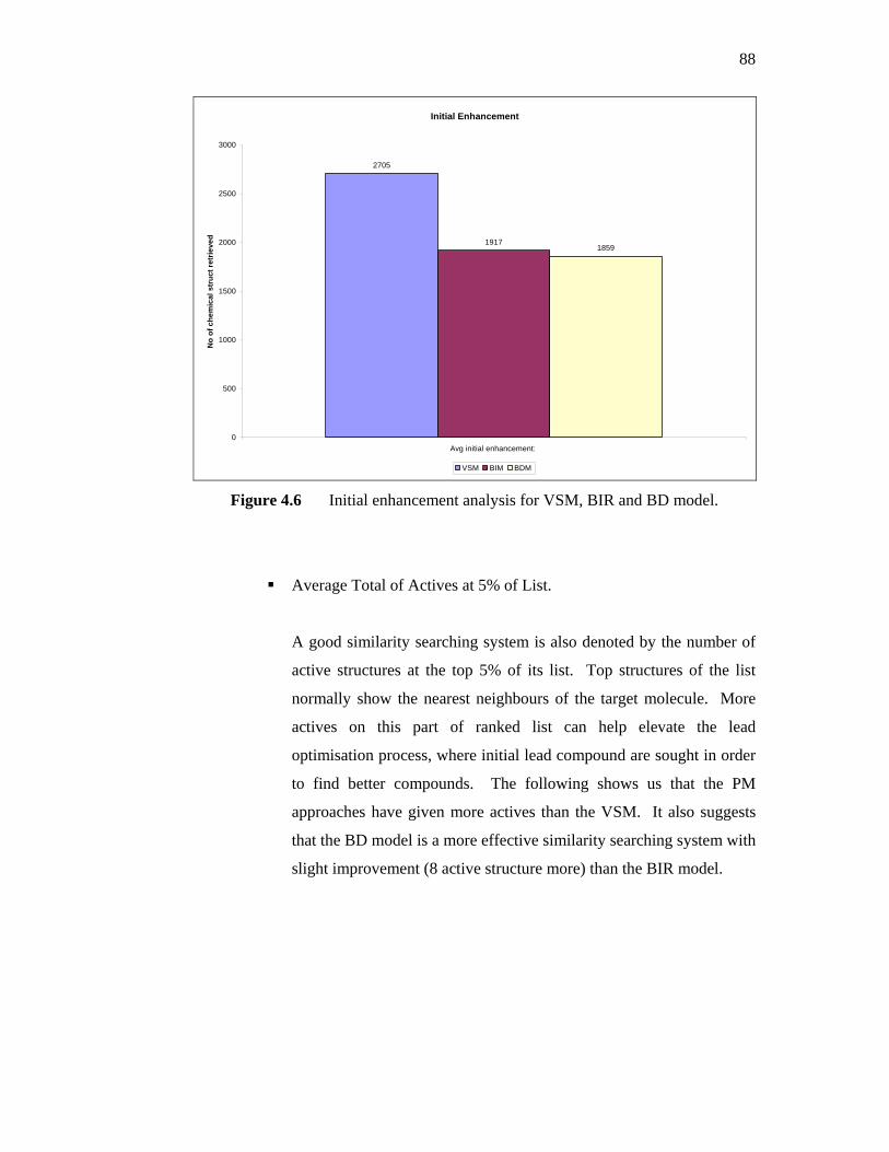
88
Initial Enhancement
2705
19171859
0
500
1000
1500
2000
2500
3000
Avg initial enhancement:
No
of c
hem
ical
str
uct r
etrie
ved
VSM BIM BDM Figure 4.6 Initial enhancement analysis for VSM, BIR and BD model.
Average Total of Actives at 5% of List.
A good similarity searching system is also denoted by the number of
active structures at the top 5% of its list. Top structures of the list
normally show the nearest neighbours of the target molecule. More
actives on this part of ranked list can help elevate the lead
optimisation process, where initial lead compound are sought in order
to find better compounds. The following shows us that the PM
approaches have given more actives than the VSM. It also suggests
that the BD model is a more effective similarity searching system with
slight improvement (8 active structure more) than the BIR model.

89
ACTIVES AT TOP 5% OF LIST
73
133
141
0
10
20
30
40
50
60
70
80
90
100
110
120
130
140
150
Avg no of actives at top 5%:
No
of a
ctiv
es s
truc
t ret
rieve
d
VSM BIM BDM Figure 4.7 Average number of actives in top 5% for VSM, BIR and BD model.
b) Experiment 2: Comparing the Performance of Query Fusion Result of
Similarity Searching Methods
Average Total of Actives at Top 400 of List.
The purpose of query fusion is to improve the performance of
similarity searching based on combining chemical target in an
iterative similarity searching to estimating probability instead of
obtaining from the entire collection. It is then compared to the
average total number of actives at top 400 of the VSM approach. A
good similarity searching system is denoted by the number of active
structures at the top 400 of its list. The following shows us that the
PM approaches have given more actives than the VSM. It also
suggests that the BD model is a more effective similarity searching
system with five active structures more than the BIR model.

90
Avg no of actives at top 400
95
155160
0
20
40
60
80
100
120
140
160
180
Avg no of actives at top 400
No
of a
ctiv
e st
ruct
ures
VSM BIR BD Figure 4.8 Average number of actives in top 400 for VSM, BIR and BD model.
4.5 Summary
The proposed approaches for similarity searching are implemented according
to the steps listed in the methodology. Based on its ranked list, evaluation is done to
determine which method is better. Four main evaluation merits were considered here
which are the GH score, initial enhancement, total actives at top 5% and total actives
at top 400. They are needed as to resolve the following issues: 1) Does PM-based
similarity searching really overcomes the existing similarity searching; and 2) Which
of the probability model proposed, perform better in the chemical database
environment. Results in this chapter have shown that in all four evaluation merits,
the PM is superior, with significant improvement over the VSM. Other than that, we
can also conclude that the theoretical stronger BD model has a slight improvement
over the BIR model, which has a weaker notion of dependence.

CHAPTER 5
CONCLUSION
5.1 Summary of Work
IR has taken the centre stage when the Internet was introduced. Now, with
endless repository of knowledge and culture, searching for information can be
tedious. Standard Boolean logic approaches are no longer sufficient for retrieving
information. Hence, many new retrieval models were introduced. VSM is currently
the most popular model used in major information services and the WWW. Current
similarity searching of chemical compounds also applies similar approach as the
vector space. Since there are similarities in the way that chemical and textual
database records are characterised, it is no wonder why algorithms developed for the
processing of textual databases can also be applied in chemical structure database
processing database.
In the effort of improving the chemical retrieval system, PM is proposed for
this project. It has strong theoretical basis and in principle should give the best
performance of relevance. Since there are no known application of probability
model in similarity searching, hence this statement is yet to be proven.

92
Among the PM approaches proposed is the BIR and BD model. BIR model
was chosen, as it is the simplest probability model there is. It was initially
considered to see whether PM could be indeed applied in the chemical database
environment. The success of the implementation of BIR model has encourage the
PM to be seriously considered for similarity searching.
PM was proposed to overcome the VSM limitations, particularly its bit
independence assumption. As the BIR model offers linked-dependence, which is a
weaker assumption of bit dependence, hence it is obvious to extend this work by
repeating experiments with a dependence model i.e. BD model.
Results from experiments carried out have determined that PM really did
perform better than the existing similarity searching. It gave better result in all the
evaluation criteria thus confirming this statement. In terms of which probability
model performs better, the BD model shown some improvement over the BIR model.
Thus, the findings of this work have help close the knowledge gap with hope that it
can help contribute to the improvement of the current similarity searching system.
5.2 Future Work
The works of this project can be further enhanced in many ways. Additional
experiments can also be carried out to validate further the findings of this project.
Since, various other techniques could be explored to find better alternatives to
current similarity searching; hence, works need to be done before a practical
implementation can be built upon the findings.

93
Take for example, there many other probability models that appeal for future
consideration. The non-binary independence model (Yu and Lee, 1986; Yu, Meng
and Park, 1989) for instance, captures the information about the number of
occurrences of a term within a document as well as the number of document having
the term. It has yield significant improvement over BIR model and is one of the
ways to alleviate the consequences of the term independence assumption. Hence,
this model should also be considered for future research. Other models such as
inference network or belief network can also be studied.
Experiments in this project could also be carried out on other chemical
database available. Chen and Reynolds (2002) mentioned that the NCI AIDS
database is not a perfect data set for evaluation but it is the best data set available.
Hence, to complement the findings, other chemical database should also be
considered. For example the MDDR (MDL Drug Data Report) database. It is a
licensable database and contains diverse drug-like molecules to which most have
been assigned a therapeutic category (Molecular Design Ltd.). As the NCI AIDS
database gives thorough sampling of a particular region in chemical space, MDDR in
turn gives a broad coverage of chemical space that is pharmaceutically relevant.
In addition, other bit string representation can also be used in this project to
represent chemical compounds, for example the Daylight fingerprint (James, el. al,
2000) and the UNITY 2D bit strings (Tripos Inc., 1999). The Daylight fingerprint is
a 2048-bit hashed fingerprint that encodes each atom’s type, augmented atoms and
paths of length 2 to 7 atoms. One of the advantages of hashed fingerprint is that it is
not library biased. However, it does experience some loss of information.
Meanwhile, UNITY 2D bit-string, unlike Daylight fingerprint that hashes all
recorded information over the whole length of the fingerprint, keeps information
from different-length paths distinct. Different parts of the bit string, record
information of fragments of length 2 to 6. A few generic structural keys are added
for some common atoms and bond types, producing a bit string of 992 bits.

94
LIST OF REFERENCE
Adamson, G.W. and Bush, J.A. (1975). A comparison of the performance of some
similarity and dissimilarity measures in the automatic classification of chemical
structures. Journal of Chemical information and Computer Science. 15:55-58.
Belkin, N.J., Kantor, P.B., Fox, E. and Shaw, J. (1995). Combining the evidence of
multiple query representations for information retrieval. Information
Processing and Management. 31: 431-448.
Bajorath, J. (2002). Virtual screening in drug discovery: Methods, expectations and
reality. Current Drug Discovery. March 2002: 24-28.
Barnard Chemical Information Ltd. (No date). Barnard Chemical Information
fingerprint. Available at: http://www.bci.gb.com.
Blair, D.C. and Maron, M.E (1985). An evaluation of retrieval effectiveness for a
full-text document-retrieval system. Communications of ACM. 28(3): 289-299.
Bollmann-Sdorra, P. and Raghavan V.V. (1998). On the Necessity of Term
Dependence in a query Space for Weighted Retrieval. Journal of the American
Society for Information Science. 49(13): 1161-1168.
Brown, R.D. and Martin, Y.C. (1997). The information content of 2-D and 3-D
structural descriptors relevant to ligand-receptor binding. Journal of Chemical
Information and Computer Sciences. 37: 1-9

97
Chen, V. and Reynolds, C.H. (2002). Performance of similarity measures in 2 D
fragment-based similarity searching: comparison of structural descriptors and
similarity coefficients. Journal of chemical Information Computer Sciences. 42:
1407-1414.
Chow, C. and Liu, C. (1968). Approximating discrete probability distributions with
dependence trees. IEEE Transactions on Information Theory, 1968. 14(3):
462-467.
Cooper, W.S. (1995). Some Inconsistencies and Misidentified Modeling
Assumption in Probabilistic Information Retrieval. ACM Transaction on
Information Systems. 13(1): 100-111.
Cooper, W.S. (1994). The formalism of probability theory in IT: A foundation or
an encumbrance?. Proceedings of the 17th Annual International ACM SIGIR
Conference on Research and Development in Information Retrieval. Dublin,
Ireland: ACM, 242-247.
Crestani F., Ruthven, I., Sanderson, M., and van Rijsbergen, C.J. (1995). The
troubles with using a logical model of IR on a large collection of documents.
Experimenting retrieval by logical imaging on TREC. Proceedings of the
Fourth Text Retrieval Conference.
Crestani F., Lalmas, M., van Rijsbergen, C.J and Campbell, I. (1998). Is This
Document Relevant?... Probably: A Survey of Probabilistic Models In
Information Retrieval. ACM Computing Surveys. 30(4): 528-552.
Croft, W.B (1995). What Do People Want from Information Retrieval? : The top
10 research issues for companies that use and sell IR systems. D-Lib Magazine.
November 1995. Available at: http://www.dlib.org/dlib/november95/
11Croft.htm.

98
Dominich, S. (2000). Formal Foundation of Information Retrieval. Proceedings of
SIGIR Workshop on Formal Mathematical Methods for Information Retrieval
2000. Athens, Greece, 69-75.
Durant J.L., Leland B.A., Henry D.R. and Nourse J.G. (2002). Re-optimization of
MDL keys for use in drug discovery. Journal of Chemical Information and
Computer Science. 42: 1273-1280.
Ellis D., Furner-Hines, J. and Willett, P. (1994). Measuring the degree of similarity
between objects in text-retrieval systems. Perspective of Information
Management. 3: 128-149.
Flower, D.R. (1997). On Properties of Bit String-Based Measures of Chemical
Similarity. Journal of Chemical Information and Computer. Science. 38:379-
386.
Fuhr, N. (1992). Probabilistic Models in Information Retrieval. The Computer
Journal. 35(3): 243-255.
Fuhr, N. (2001). Models in Information Retrieval. Springer Lecture Notes In
Computer Science Series. 21-50.
Gillet, V.J. (1999). Computational Aspects of Combinatorial Chemistry. In Fassina,
G. & Miertus, S., eds. Combinatorial Chemistry and Combinatorial
Technologies: Principles, Methods and Applications. New York: Marcel Dekker
Inc., 1999. 251-274.
Gillet, V.J., Wild, D.J., Willett, P. and Bradshaw, J. (1998). Similarity and
Dissimilarity Methods for Processing Chemical Structure Databases. The
Computer Journal. 41(8): 547-557.

99
Güner, O.F. and Henry, D.R. (1998). Formula For Determining the ‘Goodness Of
Hit List’ In 3D Database Searches. Network Science. Available at:
http://www.netsci.org/Science/Cheminform/feature09.html.
James C.A., Weininger, D. and Delany, J. (2000). Daylight Theory Manual 4.71.
Available from: http://www.daylight.com/dayhtml/doc/theory/theory.toc.html.
Johnson, M.A. and Maggiora, G.M (1990). Concepts and Application of Molecular
Similarity. John Wiley and Sons, New York.
Whitney, V.K.M. (1972). Algorithm 422: Minimal Spanning Tree.
Communications of ACM. 15(4): 273-274.
Lee, C. and Lee, G.G. (2002). Probabilistic Information Retrieval Model for
Dependency Structured Indexing System. Proceedings of ACM SIGIR
Workshop on Formal Mathematical Methods for Information Retrieval 2002.
August 12-15. Tampere, Finland.
Lee, D.L., Huei C., and Seamons, K (1997). Document ranking and the vector-
space model. Software, IEEE. 14(2): 67-75.
Losee, R.M. (1994). Term dependence: Truncating the Bahadur-Lazarsfeld
expansion. Information Processing and Managements. 30(2): 293-303.
Losee, R. M. (1997). Comparing Boolean and Probabilistic Information Retrieval
Systems Across Queries and Disciplines. Journal of the American Society for
Information Science. 48(2): 143-156.
Miller, M.A. (2002). Chemical Database Techniques in Drug Discovery. Nature
Reviews: Drug Discovery. March 2002 (1): 220-227. Available at:
http://www.nature.com/reviews/drugdisc.
Molecular Design Ltd. (No date). MDDR (MDL Drug Data Report) Database.
Available at: http://www.mdli.com.

100
National Cancer Institute (1999). Screening result October 1999. Aids Antiviral
Screen Available Public Data. Available at:
http://dtp.nci.nih.gov/docs/aids/aids_data.htm.
Patterson, D.E., Cramer, R.D., Ferguson, A.M., Clark, R.D. and Weinberger, L.E.
(1996). Neighborhood behavior: as useful concept for validation of molecular
diversity descriptors. Journal of Medical Chemistry. 39: 3060-3069.
Rajashekar, T. and Croft, W. (1995). Combining automatic and manual index
representations in probabilistic retrieval. Journal of American Society for
Information Science. 46:272-383.
Robertson, S.E. and Walker, S. (1997). On relevance weights with little relevance
information. Proceedings of the ACM SIGIR. 16-24.
Salim, N. (2002). Analysis and Comparison of Molecular Similarity Measures.
University of Sheffield: Ph.D. Thesis.
Salton, G., Buckley, C. and Yu, C.T. (1983). An Evaluation of Term Dependence
Models in Information Retrieval. Lecture Notes in Computer Science: Research
and Development in Information Retrieval. May 1983. 151-165.
Salton, G. and Buckley, C. (1988a). Parallel Text Search Methods. Communication
of the ACM. 31(2): 202-215.
Salton, G. and Buckley, C. (1988b). Term-weighting approaches in automatic
retrieval. Information Processing and Management. 24(5): 513-523.
Sheridan, R.P. (2000). The centroid approximation for mixtures: calculating
similarity and deriving structure-activity relationships. Journal of Chemical
Information and Computer Science. 40:1456-1469.
101
Sheridan, R.P. and Kearsley S.K. (2002). Why do we need so many chemical
similarity search methods? Drug Discovery Today (DDT). September 2002 (7):
903-910.
Singh, S.B., Sheridan, R.P., Fluder, E.M. and Hull, R.D. (2001). Mining the
chemical quarry with joint chemical probes: an application of latent semantic
structure indexing (LaSSI) and TOPOSIM (Dice) to chemical database mining.
Journal of Medicinal Chemistry. 44:1564-1575.
Sparck Jones, K. (1973). A statistical interpretation of term specificity and its
application to retrieval. Information storage and retrieval. 9(11): 619-633.
Tripos Inc. (1999). UNITY Reference Guide version 4.1. Tripos, St. Louis,
Missouri.
Turtle, H. and Croft, W. (1991). Evaluation of an inference network-based retrieval
model. ACM Transactions on Information Systems. 9:187-222.
van Rijsbergen, C.J. (1979). Information Retrieval. 2nd ed. University of Glasgow.
87-110.
Willett, P. (2000). Textual and chemical information processing: different domains
but similar algorithms. Information Research, 2000. 5(2). Available at:
http://informationr.net/ir/5-2/paper69.html.
Yates, R.B. and Neto, B.R. (1999). Modern Information Retrieval. England: ACM
Book Press. 224-34.
Yu, C.T., Meng, W. and Park, S. (1989). A Framework for Effective Retrieval.
ACM Transaction on Database Systems. 14(2). 147-167.

102
Yu, C.T. and Lee T.C. (1986). Non-binary independence model. Proceedings of
the 9th annual international ACM SIGIR conference on Research and
development in information retrieval. 67-75.
Yu, C.T., Lam, K. and Salton, G. (1982). Term weighting in IR using the term
precision model. Journal of the Association for Computing Machinery. 29(1):
152-170.