The Sequence Memoizer

Frank WoodCedric Archambeau

Jan GasthausLancelot JamesYee Whye Teh

Gatsby UCL

GatsbyHKUSTGatsby

Executive Summary• Model

– Smoothing Markov model of discrete sequences– Extension of hierarchical Pitman Yor process [Teh 2006]

• Unbounded depth (context length)

• Algorithms and estimation– Linear time suffix-tree graphical model identification and

construction– Standard Chinese restaurant franchise sampler

• Results– Maximum contextual information used during inference– Competitive language modelling results

• Limit of n-gram language model as n!1

– Same computational cost as a Bayesian interpolating 5-gram language model

Executive Summary• Uses

– Any situation in which a low-order Markov model of discrete sequences is insufficient

– Drop in replacement for smoothing Markov model

• Name?– ``A Stochastic Memoizer for Sequence Data’’ !

Sequence Memoizer (SM) • Describes posterior inference [Goodman et al ‘08]

Statistically Characterizing a Sequence• Sequence Markov models are usually constructed by

treating a sequence as a set of (exchangeable) observations in fixed-length contexts

oacac !

8><

>:

cjaoajcacjac

trigram

oacac !

8>>><

>>>:

ajocjaajccja

oacac !

8>>>>>><

>>>>>>:

oj[]aj[]cj[]aj[]cj[]

oacac !

(ajcaocjaca

bigramunigram 4-gram

Increasing context length / order of Markov model

Decreasing number of observations

Increasing number of conditional distributions to estimate (indexed by context)

Increasing power of model

Finite Order Markov Model

• Example

P (x1:N ) =NY

i=1

P (xi jx1; : : :xi ¡ 1)

¼NY

i=1

P (xi jxi ¡ n+1; : : :xi ¡ 1); n = 2

= P (x1)P (x2jx1)P (x3jx2)P (x4jx3) : : :

P (oacac) = P (o)P (ajo)P (cja)P (ajc)P (cja)

= G[](o)G[o](a)G[c](a)G[a](c)G[c](a)

Learning Discrete Conditional Distributions

• Discrete distribution $ vector of parameters

• Counting / Maximum likelihood estimation – Training sequence x1:N

– Predictive inference

• Example– Non-smoothed unigram model (u = ²)

G[u]

xi

i = 1 : N

G[u](X = k) = ¼k = #f ukg#f ug

P (X n+1jx1 : : :xN ) = G[u](X n+1)

G[u] = [¼1; : : : ;¼K ];K 2 j§ j

Bayesian Smoothing• Estimation

• Predictive inference

• Priors over distributions

• Net effect– Inference is “smoothed” w.r.t. uncertainty

about unknown distribution

• Example– Smoothed unigram (u = ²) xi

i = 1 : N

P (G[u]jx1:n) / P (x1:n jG[u])P (G[u])

P (X n+1jx1:n) =R

P (X n+1jG[u])P (G[u]jx1:n)dG[u] U

G[u] » Dirichlet(U); G[u] » PY (d;c;U)G[u]

A Way To Tie Together Distributions

• Tool for tying together related distributions in hierarchical models• Measure over measures• Base measure is the “mean” measure

• A distribution drawn from a Pitman Yor process is related to its base distribution – (equal when c = 1 or d = 1)

G[u] » PY (d;c;G[¾(u)])

xi » G[u]

concentrationdiscount

base distribution

E [G[u](dx)] = G[¾(u)](dx)

[Pitman and Yor ’97]

Pitman-Yor Process Continued• Generalization of the Dirichlet process (d = 0)

– Different (power-law) properties– Better for text [Teh, 2006] and images [Sudderth and Jordan,

2009]

• Posterior predictive distribution

• Forms the basis for straightforward, simple samplers• Rule for stochastic memoization

P (X N +1jx1:N ;c;d) ¼Z

P (xN +1jG[u])P (G[u]jx1:N ;c;d)dG[u]

= E

" P Kk=1(mk ¡ d)I(Ák = X N +1)

c+ N+

c+ dKc+ N

G[¾(u)](X N +1)

#

Can’t actually do this integral this way

Hierarchical Bayesian Smoothing• Estimation

• Predictive inference

• Naturally related distributions tied together

• Net effect – Observations in one context affect

inference in other context.– Statistical strength is shared between

similar contexts• Example

– Smoothing bi-gram (w = ², u,v 2 Σ)

xjxi

U£ = fG[u];G[v];G[w]g; w = ¾(u) = ¾(v)

P (£ jx1:N ) / P (x1:N j£ )P (£)

P (X N +1jx1:N )

=Z

P (X N +1j£ )P (£ jx1:N )d£

G[w]

j = 1: N[v]i = 1: N[u]

G[v]G[u]

G[theUnited States] » PY (d;c;G[United States])

SM/HPYP Sharing in Action

Conditional Distributions Posterior Predictive ProbabilitiesObservations

U

G[CP ] G[GP ]

G[P ]

G[]

CRF Particle Filter Posterior Update

Conditional Distributions Posterior Predictive ProbabilitiesObservations

CPU

U

G[CP ] G[GP ]

G[P ]

G[]

CRF Particle Filter Posterior Update

Conditional Distributions Posterior Predictive ProbabilitiesObservations

CPU

CPU

U

G[CP ] G[GP ]

G[P ]

G[]

HPYP LM Sharing Architecture• Share statistical strength

between sequentially related predictive conditional distributions– Estimates of highly specific

conditional distributions

– Are coupled with others that are related

– Through a single common, more-general shared ancestor

• Corresponds intuitively to back-off

G[]

G[a] G[the]

G[wason the]

G[on the]

G[ison the]

Unigram

2-gram

3-gram

4-gramG[wason the]G[ison the]

G[on the]

G[wason the]G[ison the]

G[the]

G[on the]

G[wason the]G[ison the]

G[wason the]

G[ison the]

G[on the]

Hierarchical Pitman Yor Process

• Bayesian generalization of smoothing n-gram Markov model • Language model : outperforms interpolated Kneser-Ney (KN) smoothing• Efficient inference algorithms exist

– [Goldwater et al ’05; Teh, ’06; Teh, Kurihara, Welling, ’08]

• Sharing between contexts that differ in most distant symbol only• Finite depth

G[] j d0;U » PY (d0;0;U)

G[u] j djuj ;G[¾(u)] » PY (djuj;0;G[¾(u)])

xi j x1:i ¡ 1 = u » G[u]

i = 1;: : : ;T

8u 2 § n¡ 1

[Goldwater et al ’05, Teh ’06]

Alternative Sequence Characterization• A sequence can be characterized by a set of

single observations in unique contexts of growing length

Increasing context length

Always a single observation

Foreshadowing: all suffixes of the string “cacao”

oacac !

8>>>>>><

>>>>>>:

oj[]ajocjaoajcaocjacao

``Non-Markov’’ Model

• Example

• Smoothing essential– Only one observation in each context!

• Solution– Hierarchical sharing ala HPYP

P (x1:N ) =NY

i=1

P (xi jx1; : : :xi ¡ 1)

= P (x1)P (x2jx1)P (x3jx2;x1)P (x4jx3; : : :x1) : : :

P (oacac) = P (o)P (ajo)P (cjoa)P (ajoac)P (cjoaca)

Sequence Memoizer

• Eliminates Markov order selection• Always uses full context when making predictions• Linear time, linear space (in length of observation sequence) graphical

model identification• Performance is limit of n-gram as n!1• Same or less overall cost as 5-gram interpolating Kneser Ney

G[] j d0;U » PY (d0;0;U)

G[u] j djuj ;G[¾(u)] » PY (djuj;0;G[¾(u)])

xi j x1:i ¡ 1 = u » G[u]

i = 1;: : : ;T

8u 2 § +

Graphical Model Trie

Observations

oacac !

8>>>>>><

>>>>>>:

oj[]ajocjaoajcaocjacao

Latent conditional distributions with Pitman Yor priors / stochastic memoizers

Suffix Trie Datastructure

oacac !

8>>>>>><

>>>>>>:

oj[]ajocjaoajcaocjacao

All suffixes of the string “cacao”

Suffix Trie Datastructure• Deterministic finite automata that recognizes

all suffixes of an input string.• Requires O(N2) time and space to build and

store [Ukkonen, 95]• Too intensive for any practical sequence

modelling application.

Suffix Tree• Deterministic finite automata that recognizes

all suffixes of an input string• Uses path compression to reduce storage and

construction computational complexity.• Requires only O(N) time and space to build and

store [Ukkonen, 95]• Practical for large scale sequence modelling

applications

Suffix Trie Datastructure

Suffix Tree Datastructure

Graphical Model Identification• This is a graphical model transformation under

the covers.• These compressed paths require being able to

analytically marginalize out nodes from the graphical model

• The result of this marginalization can be thought of as providing a different set of caching rules to memoizers on the path-compressed edges

Marginalization• Theorem 1: Coagulation

If G2jG1 » PY (d1;0;G1) and G3jG2 » PY (d2;0;G2)then G3jG1 » PY (d1d2;0;G1) with G2 marginalized out.

[Pitman ’99; Ho, James, Lau ’06; W., Archambeau, Gasthaus, James, Teh ‘09]

G1

G2

G3

→

G1

G3

Graphical Model Trie

Graphical Model Tree

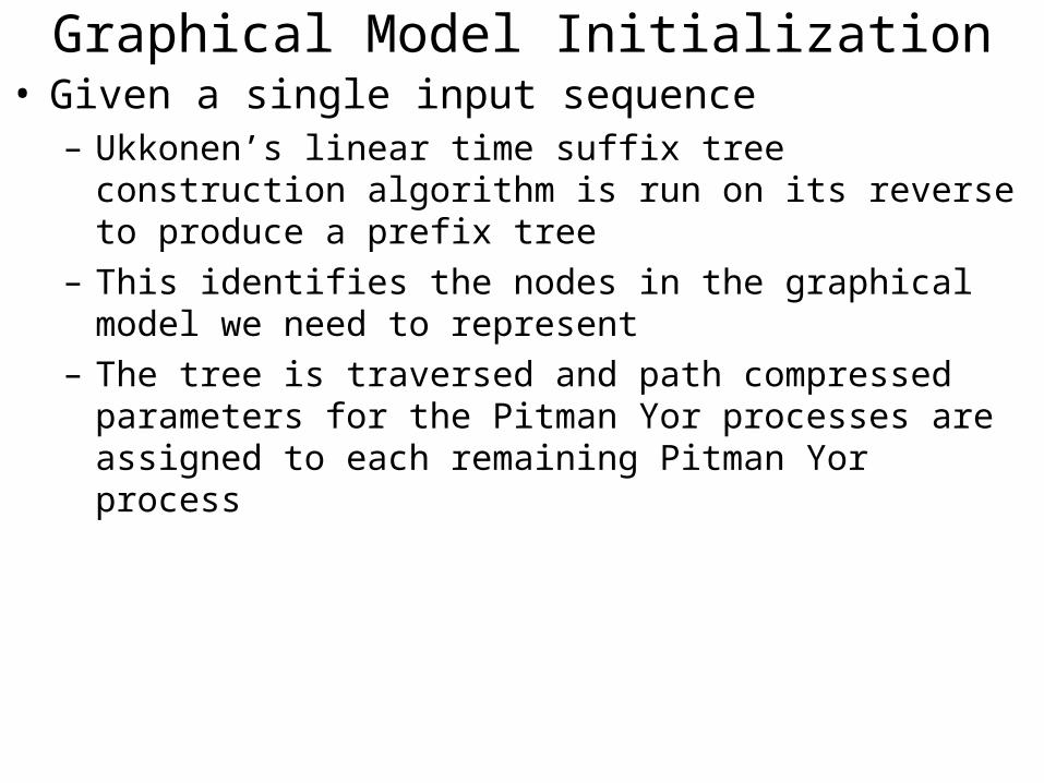
Graphical Model Initialization• Given a single input sequence

– Ukkonen’s linear time suffix tree construction algorithm is run on its reverse to produce a prefix tree

– This identifies the nodes in the graphical model we need to represent

– The tree is traversed and path compressed parameters for the Pitman Yor processes are assigned to each remaining Pitman Yor process

Nodes In The Graphical Model

Never build more than a 5-gram

Sequence Memoizer Bounds N-Gram Performance

HPYP exceeds SM computational complexity

Language Modelling Results

[Mnih & Hinton, 2009] 112.1[Bengio et al., 2003] 109.04-gram Modified Kneser-Ney [Teh, 2006] 102.44-gram HPYP [Teh, 2006] 101.9Sequence Memoizer (SM) 96.9

AP News Test Perplexity

The Sequence Memoizer• The Sequence Memoizer is a deep (unbounded)

smoothing Markov model • It can be used to learn a joint distribution over discrete

sequences in time and space linear in the length of a single observation sequence

• It is equivalent to a smoothing ∞-gram but costs no more to compute than a 5-gram