The role of vegetation, soils, and precipitation on water ...

Contents lists available at ScienceDirect

Journal of Hydrology

journal homepage: www.elsevier.com/locate/jhydrol

Research papers

The role of vegetation, soils, and precipitation on water storage andhydrological services in Andean Páramo catchmentsPatricio X. Lazoa, Giovanny M. Mosqueraa,b,⁎, Jeffrey J. McDonnellc, Patricio Crespoaa Departamento de Recursos Hídricos y Ciencias Ambientales, Facultad de Ingeniería & Facultad de Ciencias Agropecuarias, Universidad de Cuenca, Av. 12 de Abril,Cuenca, Ecuadorb Institute for Landscape Ecology and Resources Management (ILR), Research Centre for BioSystems, Land Use and Nutrition (IFZ), Justus Liebig University, Giessen,GermanycGlobal Institute for Water Security, University of Saskatchewan, Saskatoon, Canada

A R T I C L E I N F O

This manuscript was handled by Marco Borga,Editor-in-Chief, with the assistance of MichaelBruen, Associate Editor

Keywords:Andean Páramo wetlandsPassive storageDynamic storagePeatlandWater regulationEcosystem services

A B S T R A C T

Understanding how tropical montane catchments store and release water, and the resulting water ecosystemservices they provide is crucial for improving water resource management. But while research in high–elevationtropical environments has made progress in defining streamflow generation processes, we still lack fundamentalknowledge regarding water storage characteristics of catchments. Here we explore catchment storage and thefactors controlling its spatial variability in seven Páramo catchments (0.20–7.53 km2) in southern Ecuador. Weapplied a field-based approach using hydrometeorological, water stable isotopic, and soils hydrophysical datafrom a 3 year collection period to estimate the passive (PasS) and dynamic (DynS) storage of the catchments. Wealso investigated relations between these storages and landscape and hydrometric variables using linear re-gression analysis. PasS estimates from hydrophysical soil properties and soil water mean transit times wereconsistent with estimates using streamflow mean transit times. Computed catchment PasS and DynS for the sevenwatersheds were 313–617mm and 29–35mm, respectively. PasS increased directly with the areal proportion ofHistosol soils and cushion plant vegetation (wetlands). DynS increased linearly with precipitation intensity.Importantly, only 6–10% of the mixing storage of the catchments (DynS/PasS) was hydrologically active in theirwater balance. Wetlands internal to the catchments were important for PasS, where constant input of low in-tensity precipitation sustained wetlands recharge, and thus, the water regulation capacity (i.e., year–round watersupply) of Páramo catchments. Our findings provide new insights into the factors controlling the water reg-ulation capacity of Páramo catchments and other peaty soils dominated environments.

1. Introduction

Mountainous headwaters provide key water–related services fordownstream ecosystems and populations worldwide (Viviroli et al.,2007). This is particularly true for headwater tropical ecosystems(Aparecido et al., 2018; Asbjornsen et al., 2017; Hamel et al., 2017),such as the Andean Páramo, which occupies over 30,000 km2 ofnorthern South America (Hofstede et al., 2003; Wright et al., 2017) andsustains the economy of millions of people in the region (IUCN, 2002).Among the variety of ecosystem services provided by the Páramo, itshigh water production and regulation (i.e., sustained streamflow pro-duction during a water year) capacity are two of the most important(Buytaert, 2004; Poulenard et al., 2003). While recent Páramo hy-drology research has focused on the investigation of the factors

controlling the water production capacity of this ecosystem (e.g., Roa-García and Weiler, 2010; Buytaert and Beven, 2011; Crespo et al., 2011,2012, Mosquera et al., 2015, 2016a, 2016b; Correa et al., 2017; Polket al., 2017), the factors controlling its water regulation capacity havenot been yet studied in detail.Water regulation by headwater catchments is highly influenced by

their capacity to store and release water (Mcnamara et al., 2011). Assuch, in the last decade, there has been an increasing interest within thehydrological science community towards improving our understandingof catchment water storage (hereafter referred to as ‘catchment sto-rage’). For instance, the study of catchment storage has helped improveour general understanding of the streamflow–storage relationships(e.g., Spence, 2007; Soulsby and Tetzlaff, 2008; Kirchner, 2009; Soulsbyet al., 2011; Tetzlaff et al., 2014) and how storage regulation and

https://doi.org/10.1016/j.jhydrol.2019.03.050Received 26 October 2018; Received in revised form 5 March 2019; Accepted 6 March 2019

⁎ Corresponding author at: Departamento de Recursos Hídricos y Ciencias Ambientales, Facultad de Ingeniería & Facultad de Ciencias Agropecuarias, Universidadde Cuenca, Av. 12 de Abril, Cuenca, Ecuador.

E-mail addresses: [email protected], [email protected] (G.M. Mosquera).

Journal of Hydrology 572 (2019) 805–819

Available online 16 March 20190022-1694/ © 2019 Elsevier B.V. All rights reserved.

T

http://www.sciencedirect.com/science/journal/00221694

https://www.elsevier.com/locate/jhydrol

https://doi.org/10.1016/j.jhydrol.2019.03.050


mailto:[email protected]

mailto:[email protected]


http://crossmark.crossref.org/dialog/?doi=10.1016/j.jhydrol.2019.03.050&domain=pdf

storage–discharge hysteresis depends on the antecedent wetness, flowrates, and catchment scale (Davies and Beven, 2015). These findings inturn, have been extremely useful as basis for the enhancement of thestructure of hydrological models (e.g., Sayama and McDonnell, 2009;Nippgen et al., 2015; Soulsby et al., 2015; Birkel and Soulsby, 2016).Notwithstanding, direct quantification of catchment storage re-

mains difficult because of its largely unobservable nature (Hale et al.,2016) and the marked internal (i.e., subsurface) spatial heterogeneitywithin and among catchments (Seyfried et al., 2009; Soulsby et al.,2008). In response to this, different approaches such as gravimetrictechniques (Hasan et al., 2008; Rosenberg et al., 2012), cosmic ray soilmoisture observations (Heidbüchel et al., 2015), soil moisture mea-surements (Grant et al., 2004; Seyfried et al., 2009), streamflow re-cession analysis (Birkel et al., 2011; Kirchner, 2009), water balancebased (WBB), and tracer–based (TB) techniques (e.g., stable isotopes)(Birkel et al., 2011; Hale et al., 2016; Mcnamara et al., 2011) have beenapplied in order to investigate these important feature of the hydrologiccycle. Among these, the combination of techniques has proven to pro-vide the most valuable insights into water storage in catchments(Staudinger et al., 2017). The combination of WBB and TB methods, forexample, has allowed for an indirect quantification of dynamic storage(storage that is determined by the fluxes of water into and out of the

catchment over a given period of time; Sayama et al., 2011; hereafterreferred as DynS) and passive storage (the subsurface volume of waterstored within the catchment that mixes with incoming precipitation;Dunn et al., 2010; Birkel et al., 2011; hereafter referred as PasS).However, to date, only few studies have investigated storage combiningdifferent techniques (e.g., Pfister et al., 2017; Staudinger et al., 2017).Few studies too have yet quantified the relation between catchmentstorage and catchment features (e.g., rainfall temporal variability, ve-getation, soils, geology) and this remains an open question in hydro-logical science (Mcnamara et al., 2011).Most studies of catchment storage dynamics to date have been

conducted in single catchments and using only one of the aforemen-tioned storage quantification methods. The few comparative studieshave shown that soils and soil drainability play an important role oncatchment storage on Scottish peatland dominated catchments (Tetzlaffet al., 2014) and Canadian boreal wetland dominated catchments(Spence et al., 2011). In contrast, geology and topography have beenobserved to control storage dynamics in steep forested catchments withwell–drained soils in Oregon, USA (Hale et al., 2016; McGuire et al.,2005). Bedrock geology has also been found to control catchment sto-rage dynamics in 16 catchments in Luxembourg (Pfister et al., 2017);whereas catchment elevation controlled storage in 21 Alpine Swiss

Nomenclature

DynS Dynamic storageDynS(ES) Event scale DynSDynS(LT) Long–term DynSETa Actual evapotranspirationETa(cum) Cumulative ETaETo Reference evapotranspirationf conversion factor from ETo to ETai Mean annual dischargeMTT Mean transit timeP PrecipitationP(cum) Cumulative PPasS Passive storage

PasS(HP) PasS estimated from the soils’ hydrophysical propertiesPasS(Q) PasS estimated from the streamflow MTTPasS(S) PasS estimated from the soils’ MTTQ Discharge/streamflowQ(cum) Cumulative QQf Normalized fractional QS(t) Water balance based storage volume at time tSf Normalized fractional storageTB Tracer basedTTD Transit time distributionWBB Water balance basedZEO Zhurucay Ecohydrological observatoryθ Soil moisture content

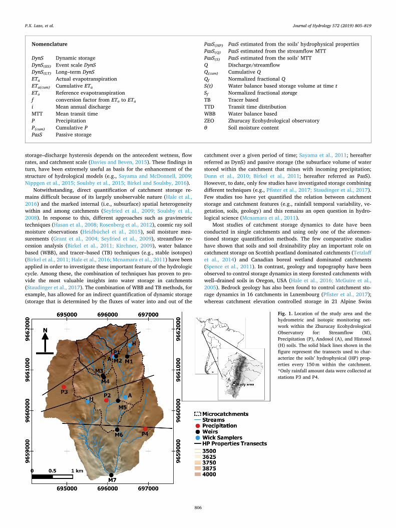
Fig. 1. Location of the study area and thehydrometric and isotopic monitoring net-work within the Zhurucay EcohydrologicalObservatory for: Streamflow (M),Precipitation (P), Andosol (A), and Histosol(H) soils. The solid black lines shown in thefigure represent the transects used to char-acterize the soils’ hydrophysical (HP) prop-erties every 150m within the catchment.*Only rainfall amount data were collected atstations P3 and P4.

P.X. Lazo, et al. Journal of Hydrology 572 (2019) 805–819

806

catchments as linked to snow versus soil water storage (Staudingeret al., 2017).Despite these recent efforts aimed at understanding storage and the

factors controlling its dynamics in several parts of the world, still thereexist many remote and understudied regions (such as the humid tro-pics) where detailed WBB and TB information are usually lacking. Herewe take advantage of a unique dataset of hydrometeorological andisotopic information collected in the nested system of headwaterAndean Páramo catchments of the Zhurucay EcohydrologicalObservatory (Mosquera et al., 2016a, 2016b; Mosquera et al., 2015).We present new WBB and TB storage estimations using these data, incombination with detailed information on the biophysical features ofthe landscape (e.g., soil type, vegetation cover, geology, topography,rainfall temporal variability) and soils’ hydrophysical properties of themonitored catchments. Our overarching question for this work is: howdo vegetation, soils, and precipitation dynamics control passive anddynamic storage across catchments? Our specific research goals s are:1) to compare different PasS calculation methods in order to validatethe TB PasS estimations; 2) to quantify the PasS and DynS of thecatchments at different temporal scales (event–based to few years); and3) to examine whether catchment features, if any, control their PasSand DynS. Information that is urgently needed to improve the under-standing of the factors that control the water-related ecosystem services(i.e., water production and regulation) provided by the Páramo and themanagement of water resources of peat-dominated catchments in tro-pical regions and elsewhere.

2. Materials and methods

2.1. Study site

The study site is the Zhurucay Ecohydrological Observatory (ZEO),located in south Ecuador. The ZEO is situated on the western slope ofthe Pacific–Atlantic continental divide within the Andean Mountainrange. The observatory expands over an altitudinal range between 3400and 3900m a.s.l. (Fig. 1). The climate is influenced by both, Atlanticand Pacific regime (Crespo et al., 2011). Mean annual precipitation is1345mm with minimal seasonality. Rainfall is composed mainly ofdrizzle year–round (Padrón et al., 2015). Mean annual temperature is6.0 °C and mean annual relative humidity is 90% at 3780m a.s.l. withinthe study site (Córdova et al., 2015).The geomorphology is dominated by glaciated U–shape valleys with

an average slope of 17%. Most of the land surface (69%) has slopes

below 20%; 5% of the catchment has slopes> 40% (Table 1; Mosqueraet al., 2015). The geology of the observatory is composed of mostlyvolcanic rocks compacted by glacial activity (Coltorti and Ollier, 2000).Two geologic formations dominate the site: (1) The late MioceneQuimsacocha formation is composed of basaltic flows with plagioclases,feldspars, and andesitic pyroclastics and (2) the Turi formation com-posed of tuffaceous andesitic breccias, conglomerates, and horizontalstratified sands.The soils in the study area are mainly Andosols and Histosols (IUSS

Working Group WRB, 2015). These soils were formed by the accumu-lation of volcanic ash over the valley bottoms and low gradient slopes.As a result of the cold, humid environmental conditions, they are black,humic, and acid soils, rich in organic matter with high water storagecapacity (Quichimbo et al., 2012). Andosols cover 76% of the ob-servatory and are mainly found on the hillslopes; while the Histosolscover the remaining 24% and are found mainly in flat areas at valleybottoms and toe slope position (Mosquera et al., 2015). Vegetation atthe study site is composed by Cushion plants (Plantago rigida, Xeno-phyllum humile, Azorella spp.), mosses, and lichens mainly covering theHistosols. Tussock grass (Calamagrostis sp.) covers the Andosols. In theZEO, as in most undisturbed Páramo areas, the areal proportion ofHistosol soils and cushion plants is strongly correlated (R2=0.74,p=0.01) and have led to the formation of “Andean wetlands”(Mosquera et al., 2016a), and hereafter we refer to them simply aswetlands.

2.2. Hydrometric information

Discharge, precipitation amount, and meteorological variables wererecorded continuously from November 2011 to November 2014.Discharge was measured in seven nested catchments. It was measuredusing V–notch weirs in catchments M1-M6 and a rectangular weir at thelargest/outlet catchment (M7, Fig. 1). The weirs were instrumentedwith Schlumberger pressure transducers with a precision of± 5mm.Water levels were recorded at a 5–minute resolution and transformedinto discharge using the Kindsvater–Shen relationship (U.S. Bureau ofReclamation, 2001). Discharge equations were calibrated using con-stant rate salt dissolution measurements (following Moore, 2004). Eventhough the use of a single rain gauge for monitoring precipitationamounts is common in headwater catchments (e.g., Buttle, 2016; Cowieet al., 2017; Pearce et al., 1986; Safeeq and Hunsaker, 2016; Sidle et al.,1995), we used 4 HOBO tipping bucket rain gauges with a resolution of0.2 mm to capture the spatial variability of precipitation within the ZEO

Table 1Landscape features and hydrometric variables of the nested system of catchments of the ZEO (From Mosquera et al., 2015).

Catchment Area (km2) Slope (%) Distribution of soil types (%) Vegetation Cover (%) Geology (%)

Andosol Histosol Tussock grass Cushion plants Polylepis Forest Pine Forest Turi Quaternary Deposits Quimsacocha

M1 0.20 14 87 13 85 15 0 0 0 0 100M2 0.38 24 85 15 87 13 0 0 1 33 66M3 0.38 19 84 16 78 18 4 0 41 0 59M4 0.65 18 80 20 79 18 3 0 48 1 50M5 1.40 20 80 20 78 17 0 4 1 30 70M6 3.28 18 78 22 73 24 1 2 30 20 50M7 7.53 17 76 24 72 24 2 2 31 13 56

Catchment Precipitation (mm y−1) Total Runoff (mm y−1) Runoff Coefficient Flow rates, as frequency of non–exceedance (l s−1 km−2)

Qmin Q10 Q30 Q50 Q70 Q90 Qmax

M1 1300 729 0.56 0.7 2.7 6.6 14.3 26.4 50.1 1039.0M2 1300 720 0.55 1.2 4.8 7.9 14.9 26.7 49.0 762.9M3 1293 841 0.65 2.3 7.3 10.8 17.7 28.1 52.4 894.2M4 1294 809 0.62 4.2 6.2 9.8 16.6 27.3 52.1 741.2M5 1267 766 0.60 1.5 4.1 8.3 15.3 26.9 50.8 905.7M6 1254 786 0.63 1.2 3.7 8.2 15.9 27.5 53.2 930.4M7 1277 864 0.68 1.9 4.0 8.7 15.2 29.2 60.8 777.9


807

(Sucozhañay and Célleri, 2018; Fig. 1). We selected these rain gaugessince they have shown to provide optimal spatial distribution of pre-cipitation within the Zhurucay Observatory with no bias and low meandaily precipitation errors (< ±0.25mm) in comparison to the use of adense network of rain gauges (n=13; Seminario, 2016). We used theKruskal-Wallis test at a statistical significance level of 0.05 to evaluatedifferences among the 3-years rainfall data recorded by the 4 rain gagesused in this study. Results from the test showed no significant differ-ences (p-value > 0.05) among the rainfall data, as has been previouslyreported in nearby Páramo areas (Buytaert et al., 2006), we applied theThiessen polygon method to these data to estimate precipitation at eachof our seven monitored catchments.Meteorological variables were also recorded using a Campbell

Scientific meteorological station co-located with the tipping bucket P1(Fig. 1). Air temperature and relative humidity were recorded with aCS–215 probe protected with a radiation shield. Wind speed was re-corded using a Met–One 034B Windset anemometer and solar radiationwas recorded with a CS300 Apogee pyranometer. We estimated re-ference evapotranspiration (ETo) for each of our study catchments usingthe FAO–56 Penman–Monteith equation (Allen et al., 1998). For thispurpose, we used the near-surface air temperature lapse rate de-termined by Córdova et al. (2016) in a nearby Páramo area to correctfor differences in air temperature with elevation at each of our catch-ments. No corrections for wind speed, relative humidity, and solar ra-diation were carried out considering the size of the study area(< 10 km2) and that these environmental variables have shown onlylimited influence on ETo estimations within the study area (Córdovaet al., 2015).

2.3. Characterization of the soils’ hydrophysical properties

Given that the sampling of soils in the study area is labor intensivedue to the harsh environmental conditions, we selected three transects(Fig. 1) to collect soil samples for soil properties analyses. Since thephysiographic position along the landscape, i.e., valley bottom, toeslope, lower slope, middle slope, upper slope, and hilltop (followingFAO, 2009; Schoeneberger et al., 2012), has shown to influence thespatial variability of soil properties in the Páramo (Guio Blanco et al.,2018); the transects were selected to capture this variability amongphysiographic positions within the catchment. Soil samples were col-lected at 45 sampling locations (in total) almost equally distributedevery 150m along the selected transects to capture the variability of thesoil properties at different physiographic positions. At each samplinglocation, we characterized the soil depth, soil types, soil horizons (or-ganic and mineral), and the thickness of each horizon. As the presenceof Andosol and Histosol soils dominates in our study area, we used thecriteria of the IUSS Working Group WRB (2015) to classify their hor-izons’ types. For both soil types, the organic horizon corresponded tosoils with organic matter contents higher than 5% and bulk densitieslower than 0.90 g cm−3, whereas the mineral horizon presented organicmatter contents lower than 5% and bulk densities higher than0.9 g cm−3.Additionally, we collected three undisturbed soil samples of

100 cm3 using steel rings (5 cm diameter) at each sampling location andsoil horizon. Following collection, the samples were saturated via ca-pillary rise from a saturated sand support for analysis of the soil watertension–water content (θ) relationships at saturation (pF 0) and fieldcapacity (pF 2.54) at the Soil Hydrophysics Laboratory of the Universityof Cuenca. The θ at saturation was obtained via gravimetry after thesaturated samples were dried up in an oven at 105 °C for 24 h and atfield capacity via the ceramic plates system method (USDA and NRCS,2004). The θ values are reported as volumetric moisture (cm3 cm−3).

2.4. Collection and analysis of isotopic data

Weekly water samples for oxygen–18 (18O) isotope analysis were

collected for the period May 2012–May 2014. These samples werecollected in streamflow, precipitation, and soil water. Grab samples instreamflow were collected at the same stations used for measuringdischarge. Given the potential spatial variability of the isotopic com-position of rainfall (Fischer et al., 2017), water samples in precipitationwere collected using two rain collectors located at 3780 and 3700ma.s.l. (P1 and P2 in Fig. 1, respectively). Precipitation water sampleswere collected using circular funnels connected to polypropylene raincollectors covered with aluminum foil and with a 5mm mineral oillayer to reduce evaporation of the stored water (IAEA, 1997). Onceprecipitation samples were collected, the rain collectors were cleaned,dried, and the mineral oil replaced before their re–installation.Soil water samples were collected using wick samplers installed at

four locations (2 Histosols and 2 Andosols) (Fig. 1). The wick samplerswere built with 9.5mm–diameter fiberglass wicks connected to apolypropylene container of 30× 30 cm (following Boll et al., 1991,1992; Knutson et al., 1993) One end of the wick was connected to thewick sampler and the other to a 1.5 L glass bottle where the soil waterwas collected and stored. In order to collect the mobile soil waterfraction (Landon et al., 1999), we applied 1m length of suction (Holderet al., 1989). The wick samplers were installed at three depths at all soilwater sampling stations. In the Histosols, they were placed at 25 and45 cm depths in the organic horizon and at 75 cm depth in the orga-nic–mineral horizons interface. In the Andosols, they were placed at 25and 35 cm depths in the organic horizon and at 65 cm depth in theshallowest part of the mineral horizon. The wick samplers in the His-tosols were located in flat zones at the valley bottoms near the streams,whereas in the Andosols they were located at the middle and bottomparts of a hillslope. Rainfall and soil water samples were filtered using0.45 µm filters in order to minimize organic matter contamination. Thecollected water samples were stored in 2ml amber glass bottles, cov-ered with parafilm, and kept away from sunlight to minimize anyfractionation by evaporation.A cavity ring–down spectrometer (Picarro L1102–i) was used to

measure the δ 18O isotopic composition of the water samples with a0.1‰ precision. To diminish the memory effect in the analyses (Pennaet al., 2012) and considering that this effect increases when samplesfrom different water types (e.g., precipitation, streamflow, soil water,groundwater) are analyzed together in individual runs, we analyzedwater samples of the same type in each run to minimize the memoryeffect. In addition, we applied six sample injections and discarded thefirst three as recommended by the manufacturer to further reduce thiseffect. For the last three injections, we calculated the maximum δ18Oisotopic composition difference and compared it with the analyticalprecision given by the manufacturer and the standard deviation of theisotopic standards used for the analyses (0.2‰ for oxygen-18). Samplesthat showed measurement differences larger than this value were re-analyzed. Contamination of the isotopic signal was checked usingChemCorrect 1.2.0 (Picarro, 2010). This evaluation showed that only 3soil samples (0.5% of the total) were contaminated with organic com-pounds. Those samples were excluded from the analysis. Isotopic con-centrations are presented in the δ notation and expressed in per mill(‰) according to the Vienna Standard Mean Ocean Water (V–SMOW;Craig, 1961).

2.5. Soil water mean transit time (MTT)

Mean transit time is defined as the time it takes for a water moleculeto travel subsurface in a hydrologic system (McGuire and McDonnell,2006). That is, from the time it enters as precipitation or snow to thetime it exists at an outlet point (e.g., streamflow, spring, soil wicksampler, or lysimeter). The approach used to estimate soil water MTTwas based on the lumped convolution method (Maloszewski and Zuber,1996), which assumes a steady–state condition of the flow system. Eventhough the steady–state assumption has been criticized as an unrealisticcatchment representation in a variety of environments, the particular


808

catchment features (i.e., relatively homogeneous soil distribution andcompact geology) and low seasonal variation of hydrometeorologicalconditions at the ZEO, justify this assumption in our study catchmentMosquera et al. (2016b). This method transforms the input tracer signal(precipitation or snowmelt; δin) into the output tracer signal (stream,soils; δout):

=(t)g( )w(t ) (t )d

g( )w(t )dout0 in

0 (1)

where, τ is the integration variable representing the MTT of the tracer,(t ) is the time lag between the input and output tracer signals, g( )is the transit time distribution (TTD) that describes the tracer’s sub-surface transport, and w(t) is a recharge mass variation function. Thelatter was applied to take into account the temporal variability in re-charge rates by weighting the input isotopic composition based onprecipitation amounts (McGuire and McDonnell, 2006). As precipita-tion isotopic composition varies as a function of elevation within thestudy site, the precipitation input signal for each catchment was cor-rected using the isotopic lapse rate determined for the ZEO. That is, anincrease of 0.31‰ in δ18O per 100m decrease in elevation (Mosqueraet al., 2016a) We used this isotopic lapse rate and the mean elevation ofeach study catchment to correct the weekly isotopic data obtained fromour two rain gauges used to monitor the input isotopic signal in ourstudy catchment (Mosquera et al., 2016b).We tested five TTDs for the simulations: the exponential model

(EM), exponential–piston flow model (EPM), the dispersion model (DM)(Małoszewski and Zuber, 1982), the gamma model (GM) (Kirchneret al., 2000), and the two parallel linear reservoir model (TPLR) (Weileret al., 2003). Similarly to the findings of Mosquera et al. (2016b) duringthe evaluation of streamflow MTTs at the ZEO, the TTD that best re-presented the subsurface transport of water through the soils was theEM. Therefore, the soil water MTTs reported below correspond to theestimations based on this TTD.

2.6. Passive storage estimations

We define passive storage as:

=PasS MTT i (2)

where: i is the mean annual discharge over the period MTT was esti-mated for each catchment or soil horizon. We estimated PasS based onthe streamflow MTTs (Table 2) of the nested system of catchments re-ported by Mosquera et al. (2016b) using the same methodology de-scribed in the Section 2.5, and hereafter referred as PasS(Q).We also approximated the PasS at the outlet of the basin (M7) based

on two additional methodologies in order to examine how much of thecatchments’ PasS(Q) is represented by the soils. The first approach wasbased on the soils’ hydrophysical properties (hereafter referred asPasS(HP)). Given the high water retention capacity of the Páramo soilsand the sustained year–round rainfall at the study site (Padrón et al.,2015), we assumed that their soil moisture content remained high andnear saturation conditions throughout the year (Buytaert, 2004). Wealso assumed that the contribution of the soils to the catchment PasS

should be between saturation and field capacity. As such, we used theθs at pF 0 (saturation) and pF 2.54 (field capacity) to estimate the waterstorage for each soil horizon at each of the positions where these soils’hydrophysical properties were measured along the landscape as fol-lows:

=PasS dHP j k j k j k( , ) ( , ) ( , ) (3)

where PasS(HP) represents the soil water storage and d the re-presentative depth of the soil horizon j (i.e., organic or mineral) atposition k across the landscape (i.e., from valley bottom to hilltop)where soil moisture θ (at saturation or field capacity) was measured.Using this approach and mapping the landscape surface that corre-sponded to the different positions k, we estimated the water storage inthe soils at each of these positions for the whole catchment. For ex-ample, for estimating the PasS(HP) of the catchment at the middle of theslope, we mapped the area of the whole catchment corresponding to aslope of 32–40% and with Andosol soil type (as indicated in Table 3).The total catchment PasS(HP) was then calculated as the sum of PasS(HP)at all monitoring positions for both the organic and mineral horizons atsaturation and field capacity.The second approach was based on the soil water MTT estimations

(hereafter referred as PasS(S)). The average of the volume of waterstored in the bottles used for the weekly collection of soil water sampleswas used to estimate the i (discharge) value in Eq. (2). This volume wasconverted to discharge by dividing it to the area of the samplers(30 cm×30 cm).In this way, we estimated the PasS(S) for each soil typeat each monitoring depth and position within the landscape. Given thatthe tracer signal at an outlet point within a catchment accounts for themixing of all the flow paths above such points (McGuire andMcDonnell, 2006), this approach represents directly the storage of allthe water draining down towards the outlet point. Consequently, nofurther integration of different landscape units is needed. This contrastswith the other alternative method where PasS(HP) requires an integra-tion of the water stored at different parts of the landscape.

2.7. Dynamic storage estimation

The WBB volumes of water stored in the catchments were estimatedfor each day during the study period following Sayama et al. (2011):

=S t P t Q t ET t( ) ( ) ( ) ( )a (4)

where: S(t), P(t), Q(t) and ETa(t) are the storage volume, precipitation,streamflow, and actual evapotranspiration at time t, respectively. Thelong–term DynS (hereafter referred as DynS(LT)) of the nested catch-ments was then defined as the difference between the maximum (Smax)and the minimum (Smin) daily storage volumes obtained from Eq. (3)over the period of analysis.Actual evapotranspiration was estimated as:

=ET f ETa o (5)

where: ETo is the potential evapotranspiration, and f is a factor whichwas calculated as the result of the difference between P and Q dividedby ETo (i.e., (P–Q)/ETo) for each catchment (Staudinger et al., 2017).

Table 2Streamflow TB Passive (PasS(Q)) and long–term Dynamic Storage (DynS(LT)) estimations for the nested system of catchments at the ZEO using data collected in theperiod Nov 2011–Nov 2014. *Catchments’ MTTs estimations were obtained from Mosquera et al., 2016b.

Catchment Streamflow MTTs* (days) Passive Storage (mm) Dynamic Storage (mm) Dynamic Storage/Passive storage (%)

M1 194 (171–227) 394 (341–453) 34 (31–37) 9M2 156 (137–186) 313 (270–361) 31 (28–34) 10M3 264 (232–310) 617 (534–714) 35 (32–38) 6M4 240 (212–280) 539 (470–621) 33 (31–36) 6M5 188 (165–219) 400 (346–460) 32 (29–35) 8M6 188 (164–220) 411 (353–474) 31 (29–34) 8M7 191 (167–224) 457 (395–530) 29 (26–32) 6


809

2.8. Runoff events selection and variables

We selected rainfall–runoff events for the analysis of the temporalvariability of DynS at the event scale (hereafter referred as DynS(ES)).These events were defined as runoff response to rainfall inputs wheredischarge increased from below low flow values (Smakhtin, 2001) –below Q35 non–exceedance flow rates (determined as low flows at theZEO, Mosquera et al., 2015) – to values higher than this thresholdduring the duration of the events. We further used the minimum inter-event time criteria, defined as the minimum time lapse without pre-cipitation between two consecutive events (Dunkerley, 2008), to se-parate the precipitation time series into rainfall events. Given that atthe study region rainfall occurs frequently and is sustained along theyear (Padrón et al., 2015), we selected a minimum inter-event time of6-hr to define independent events. Although rainfall–runoff events wereevaluated at all catchments, only the results for the outlet of thecatchment (M7) are reported as similar trends for all catchments werefound. Under these considerations, 42 events were selected for theanalysis at M7.For each event, we evaluated the storage–discharge hysteresis. This

was conducted by visual inspection of the plots of the normalizedfractional storage Sf and fractional discharge Qf (Davies and Beven,2015). These values are defined as the storage and discharge volumes asfractions of the PasS(Q) (i.e., Sf= S/PasS(Q) and Qf=Q/PasS(Q), re-spectively), where S and Q are the same as in Eq. (3), but estimated at5–minute temporal resolution for the analysis at the event scale.Additionally, we also estimated the cumulative Q (Q(cum)), cumu-

lative P (P(cum)), cumulative ETa (ETa(cum)), the minimum, mean, andmaximum rainfall intensity, as well as the antecedent wetness condi-tions of the catchment represented as the amount of antecedent pre-cipitation over different time periods (7 and 14 days before each event)for each of the 42 events to investigate the influence of these hydro-meteorological variables on DynS(ES).

2.9. Statistical analysis between storage and landscape–hydrometricfeatures

We conducted a Pearson linear correlation analysis between theestimates of PasS(Q) and DynS(LT) and different landscape featureswhich included: catchment area, soil type, vegetation cover, geology,and average slope of each catchment. We also conducted a linear

correlation analysis between PasS(Q) and DynS(LT) with hydrometricvariables that included mean annual P, mean annual Q, mean annualETa, runoff coefficient (Q/P), and different non–exceedance flow ratesaccording to the catchment’s flow duration curves. The biophysical andhydrometric features of the catchments were obtained from Mosqueraet al. (2015) (Table 1).At the event scale, linear correlation analysis was used to investigate

relations between DynS(ES) with all the hydrometeorological variablesestimated for the rainfall–runoff events (Section 2.8). All correlationswere evaluated using the determination coefficient (R2) at a statisticalsignificance level of 0.10 (i.e., 90% confidence level) using the t–stu-dent test.

3. Results

3.1. Catchment water passive storage

3.1.1. Streamflow MTT based catchment passive storage estimationsThe PasS(Q) variation among the catchments was relatively large

(304mm). These estimates varied from 313 to 617mm, with a value of457mm at the outlet of the basin (M7). The maximum values wereobserved at catchments M3 and M4, while the minimum value at M2(Table 2).

3.1.2. Hydrophysical soil properties based catchment passive storageestimationsThe hydrophysical properties of the soils (i.e., θ at pFs 0 and 2.54)

located at the different landscape positions and their areal extent withinthe ZEO are presented in Table 3. The Histosols were only found at thevalley bottom and toe slope positions. Their average thickness was70 cm for the organic horizon and 50 cm for the mineral horizon. His-tosols were normally found in low relief areas with slopes between 1and 15%. They presented the highest θs at saturation (pF 0) for theorganic (0.89–0.90 cm3 cm−3) and the mineral horizon (0.65 cm3

cm−3). The organic horizon of the Histosols had significantly higher θsat field capacity (pF 2.54; 0.62–0.63 cm3 cm−3) in comparison to themineral horizon (0.54 cm3 cm−3). The Andosols on the other hand,were found from the toe slope to the summit positions with slopesbetween 1 and 56%. Their thickness was more variable than for theHistosols, and ranged between 30 and 40 cm for the organic horizonand 20–30 cm for the mineral horizon. The θ values at saturation of the

Table 3Hydrophysical properties for each soil type, horizon, and position within the ZEO and passive storage estimations based on these properties (PasS(HP)) in relation tothe areal extent of each of them with respect to the total basin area, M7. PasS(HP) estimates were calculated for the soils’ moisture contents (θ) at field capacity (FC, pF2.54) and saturation (Sat, pF 0) conditions. *As a percentage of total catchment area (7.53 km2). **Total PasS(HP) per soil type (Andosol and Histosol soils) and horizon(organic and mineral).

Hillslope position Soil type Slope Soil thickness Area* Number of samples θFC θSat PasS(HP) Total**

FC Sat FC Sat(%) (cm) (%) (cm3 cm−3) (cm3 cm−3) (mm) (mm) (mm) (mm)

Organic Horizon Valley bottom Histosol 1–5 70 0.9 27 0.62 0.90 17 24 441 623Toe slope Histosol 5–15 70 23.1 5 0.63 0.89 424 599

Andosol 40 3.5 5 0.62 0.72 11 13 230 264Lower slope Andosol 15–32 30 22.0 5 0.67 0.83 58 72Middle slope Andosol 32–40 35 33.3 10 0.69 0.76 106 117Upper slope Andosol 40–56 38 7.8 5 0.65 0.74 25 29

Andosol > 56 38 5.6 4 0.65 0.74 18 21Summit Andosol 1–5 34 3.7 7 0.65 0.73 11 12

Mineral Horizon Valley bottom Histosol 1–5 50 0.9 27 0.54 0.65 10 13 270 325Toe slope Histosol 5–15 50 23.1 5 0.54 0.65 260 312Toe slope Andosol 30 3.5 5 0.50 0.53 7 7 131 156Lower slope Andosol 15–32 30 22.0 5 0.46 0.56 40 49Middle slope Andosol 32–40 30 33.3 10 0.46 0.56 61 74Upper slope Andosol 40–56 20 7.8 5 0.46 0.53 9 11

Andosol > 56 20 5.6 4 0.46 0.53 7 8Summit Andosol 1–5 31 3.7 7 0.46 0.53 7 8


810

organic horizon of the Andosols (0.72–0.83 cm3 cm−3) were morevariable than those of their mineral horizon (0.53–0.56 cm3 cm−3). Forboth horizons, these values were significantly lower than for the His-tosols. Their θ values at field capacity for the organic horizon of thesesoils (0.62–0.69 cm3 mm−3) were more variable and higher than thosefor their mineral horizons (0.46–0.50 cm3 cm−3).The PasS(HP) was variable among the different soil types and hor-

izons at the different positions in the landscape (Table 3). The PasS(HP)estimations using these soil properties and the spatial distribution andthickness of each soil horizon showed that the Histosols stored a higheramount of water (711mm at FC and 948mm at saturation) than theAndosols (361mm at FC and 420mm at saturation) (Table 4). In-tegrating these PasS(HP) values to the catchment scale using the arealproportions of the catchment covered by each soil type, the PasS(HP) atthe outlet of the basin (M7) were 445mm at field capacity and 547mmat saturation (Table 4).

3.1.3. Soil water MTT based catchment passive storage estimationsSoil water MTTs for Andosols and Histosols at the three monitored

depths are reported in Table 5. The MTTs in both soil types increasedwith depth. MTTs in the Andosols were 35 and 48 days for the shal-lower organic horizons and 144 days for the organic–mineral horizonsinterface. MTTs in the Histosols were longer than in the Andosols, withvalues of 212 and 292 days for the shallower organic horizons and338 days for the organic–mineral horizon interface. With these MTTvalues we estimated the PasS(S) for each soil type at each monitoringdepth (Table 5). Andosols showed PasS(S) values ranging between 14and 49mm, with the highest contribution from the mineral horizon (at65 cm depth). Histosols showed higher PasS(S) values. Similar to the soilwater MTTs, these values increased with depth. PasS(S) was 191 and263mm at the shallower organic horizons and 304mm at the orga-nic–mineral horizon interface (at 65 cm depth). Based on the PasS(S)values at each soil type and horizon, the water storage was 97mm forthe Andosols and 759mm for the Histosols.

3.2. Catchment water dynamic storage

3.2.1. Long-term dynamic storage estimationsThe catchments DynS(LT) ranged from 29 to 35mm, showing little

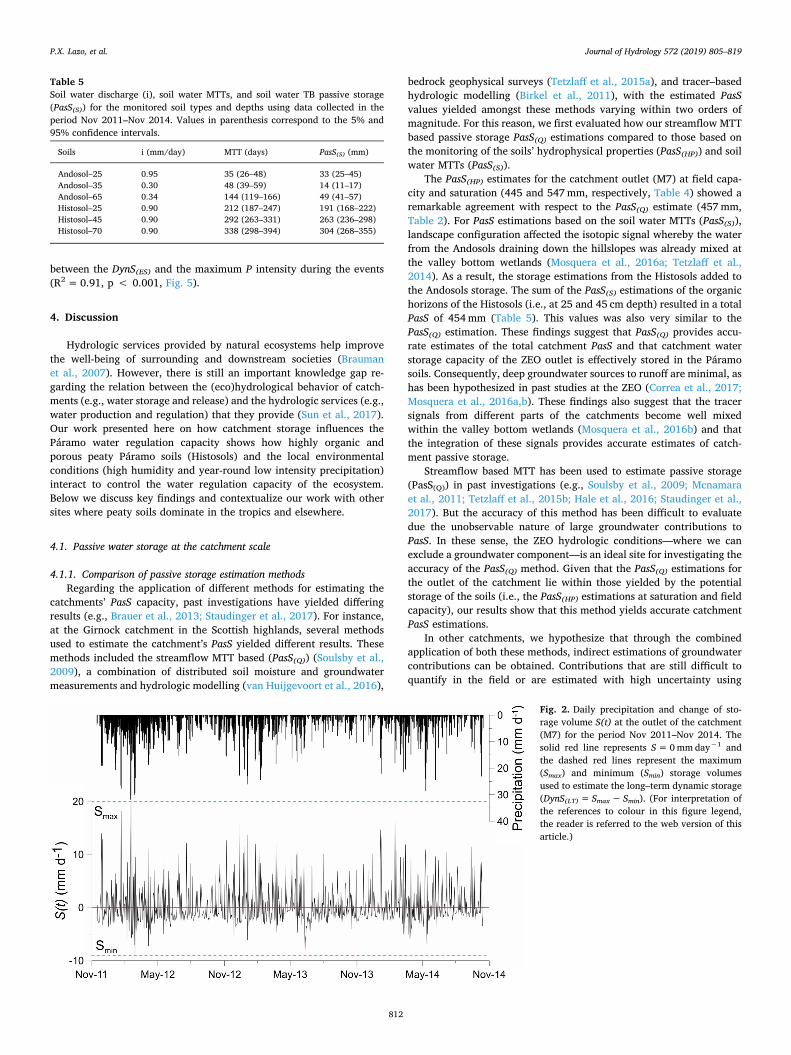
differences among subcatchments (6mm). Similar to the PasS(Q),catchments M3 and M4 showed the maximum values, while theminimum value corresponded to M7. The fractions of DynS(LT) toPasS(Q) varied between 6 and 10% among the catchments (Table 2).Fig. 2 shows the daily temporal variability of the WBB catchments’

water storage volume. The system showed a very flashy response ofstorage volume to precipitation but normally returned to a conditionwith S(t) of approximately 0mmday−1. Negative values (S(t) < 0mmday−1; when the system loses or discharges higheramounts of water than the inputs) and positive values (S(t) > 0mmday−1; when the system gains or receives higher amountsof water than it discharges) occurred at approximately the same fre-quency (53 and 47%, respectively).

3.2.2. Event-based dynamic storage estimationsThe 42 rainfall–runoff events selected for the analysis represented a

wide variety of hydrometeorologic conditions during the study period.The P(cum) at the end of the events ranged between 0.2 and 56.0mm;with Q(cum) varying between 1.2 and 52.8mm, ETa(cum) between 0.1 and16.6mm, and DynS(ES) between 0.07 and 1.91mm. In addition, max-imum, mean, and minimum P intensities during the events were in therange of 0.6–22.3mmh−1, 0.1–5.4mmh−1, and 0 to 1.1mmh−1, re-spectively. Antecedent P for 7 and 14 days prior to the start of theevents ranged between 2.6 and 68.5mm and 15.8–113.3mm.The temporal variability of Sf during the events was similar for all

catchments. A representative storm for the catchment (M7) outlet isshown in Fig. 3. The event had a total duration of 50 h and during this

period P(cum) and Q(cum) were 32.2 and 32.3mm, respectively. Fig. 3shows that at the beginning of the event (t0), the system was neitherstoring nor releasing water (with Sf=0). During the first 17.7 h (t1) ofthe event, 82% of the P(cum) entered to the system. During this hydro-graph rising limb (black line in Fig. 3a), the catchment both releasedwater via Q in response to the P inputs but was also dynamically re-charged (Sf > 0mm). Thereafter, and once rainfall intensity decreased,the system continued to change from a diminished recharge state to areleasing water state until t2 at around 18.3 hr. This period of water lossfrom the catchment was mostly linear. The hydrograph peak (t2) wasmostly caused by contribution of the moisture from the rechargedsystem rather than from precipitation inputs directly (i.e. the black linein the negative region of the Sf during the t1–t2 period in Fig. 3b). Afterrainfall cessation, the release of water from the catchment continueduntil t3 (18.6 h). At this point, the hydrograph recession decreasedlinearly until the end of the event, when the system again reached astability condition (Sf≈0mm) at 50 h (tf). The Sf dynamics at the eventscale formed an anticlockwise hysteretic loop. All of the monitoredevents at all catchments followed the same hysteretic direction.

3.3. Relations between storage metrics and landscape features andhydrometric variables

The PasS(Q) for our nested catchments was significantly positivelycorrelated with mean annual Q (R2= 0.73, p=0.07), runoff coeffi-cient (R2= 0.75, p=0.06), and high flows represented by the Q90non–exceedance flows (R2=0.67, p=0.09) (Table 6). PasS(Q) was alsosignificantly positively correlated with the cushion plants vegetationcover (R2=0.68, p=0.08) and negatively correlated with the tussockgrass vegetation cover (R2=0.73, p=0.07) (Fig. 4). Even though si-milar correlation trends were found between the catchments’ PasS(Q)and their soils’ areal extent (i.e., positive for the Histosols and negativefor the Andosols), these correlations were not statistically significant(R2 < 0.55, p > 0.15). The latter was most likely as a result of thehigher uncertainty in the soil type distribution mapping of the ZEO inrelation to the vegetation distribution mapping that was better char-acterized directly in the field (Mosquera et al., 2015).For the DynS(LT) estimations calculated from the daily WBB analysis,

we found statistically significant correlations with landscape and hy-drologic variables. However, due to the small range of variation ofDynS(LT) among catchments (only 6mm, Table 2), we acknowledge thatthese correlations may not be causal and thus do not report them. Onthe short term, when analyzing correlation between hydro-meteorological variables and the DynS(ES) during the events monitoredat the outlet of the basin, M7, we identified non–significant correlationsbetween this storage metric and most hydrometeorological variables(R2≤ 0.30, p > 0.10). These variables included the P(cum), Q(cum),ETa(cum), mean and minimum P intensities, and 7 and 14 days accu-mulated antecedent P. The only significant correlation found was

Table 4Passive storage estimations based on the soils’ hydrophysical properties(PasS(HP)) at field capacity (FC) and saturation (Sat) for the organic and mineralhorizon of the Andosols and Histosols (Table 3) and the integration of thesestorages to the catchment outlet, M7, based on the areal extent of each soil typewithin the ZEO. *Total PasS(HP)=Organic horizon PasS(HP)+Mineral horizonPasS(HP).

FC Sat(mm) (mm)Histosol Andosol Histosol Andosol

Organic horizon 441 230 623 264Mineral horizon 270 131 325 156Total PasS(HP)* 711 361 948 420Soil type percentage (%) 24 76 24 76Catchment PasS(HP) 445 547


811

between the DynS(ES) and the maximum P intensity during the events(R2= 0.91, p < 0.001, Fig. 5).

4. Discussion

Hydrologic services provided by natural ecosystems help improvethe well-being of surrounding and downstream societies (Braumanet al., 2007). However, there is still an important knowledge gap re-garding the relation between the (eco)hydrological behavior of catch-ments (e.g., water storage and release) and the hydrologic services (e.g.,water production and regulation) that they provide (Sun et al., 2017).Our work presented here on how catchment storage influences thePáramo water regulation capacity shows how highly organic andporous peaty Páramo soils (Histosols) and the local environmentalconditions (high humidity and year-round low intensity precipitation)interact to control the water regulation capacity of the ecosystem.Below we discuss key findings and contextualize our work with othersites where peaty soils dominate in the tropics and elsewhere.

4.1. Passive water storage at the catchment scale

4.1.1. Comparison of passive storage estimation methodsRegarding the application of different methods for estimating the

catchments’ PasS capacity, past investigations have yielded differingresults (e.g., Brauer et al., 2013; Staudinger et al., 2017). For instance,at the Girnock catchment in the Scottish highlands, several methodsused to estimate the catchment’s PasS yielded different results. Thesemethods included the streamflow MTT based (PasS(Q)) (Soulsby et al.,2009), a combination of distributed soil moisture and groundwatermeasurements and hydrologic modelling (van Huijgevoort et al., 2016),

bedrock geophysical surveys (Tetzlaff et al., 2015a), and tracer–basedhydrologic modelling (Birkel et al., 2011), with the estimated PasSvalues yielded amongst these methods varying within two orders ofmagnitude. For this reason, we first evaluated how our streamflow MTTbased passive storage PasS(Q) estimations compared to those based onthe monitoring of the soils’ hydrophysical properties (PasS(HP)) and soilwater MTTs (PasS(S)).The PasS(HP) estimates for the catchment outlet (M7) at field capa-

city and saturation (445 and 547mm, respectively, Table 4) showed aremarkable agreement with respect to the PasS(Q) estimate (457mm,Table 2). For PasS estimations based on the soil water MTTs (PasS(S)),landscape configuration affected the isotopic signal whereby the waterfrom the Andosols draining down the hillslopes was already mixed atthe valley bottom wetlands (Mosquera et al., 2016a; Tetzlaff et al.,2014). As a result, the storage estimations from the Histosols added tothe Andosols storage. The sum of the PasS(S) estimations of the organichorizons of the Histosols (i.e., at 25 and 45 cm depth) resulted in a totalPasS of 454mm (Table 5). This values was also very similar to thePasS(Q) estimation. These findings suggest that PasS(Q) provides accu-rate estimates of the total catchment PasS and that catchment waterstorage capacity of the ZEO outlet is effectively stored in the Páramosoils. Consequently, deep groundwater sources to runoff are minimal, ashas been hypothesized in past studies at the ZEO (Correa et al., 2017;Mosquera et al., 2016a,b). These findings also suggest that the tracersignals from different parts of the catchments become well mixedwithin the valley bottom wetlands (Mosquera et al., 2016b) and thatthe integration of these signals provides accurate estimates of catch-ment passive storage.Streamflow based MTT has been used to estimate passive storage

(PasS(Q)) in past investigations (e.g., Soulsby et al., 2009; Mcnamaraet al., 2011; Tetzlaff et al., 2015b; Hale et al., 2016; Staudinger et al.,2017). But the accuracy of this method has been difficult to evaluatedue the unobservable nature of large groundwater contributions toPasS. In these sense, the ZEO hydrologic conditions—where we canexclude a groundwater component—is an ideal site for investigating theaccuracy of the PasS(Q) method. Given that the PasS(Q) estimations forthe outlet of the catchment lie within those yielded by the potentialstorage of the soils (i.e., the PasS(HP) estimations at saturation and fieldcapacity), our results show that this method yields accurate catchmentPasS estimations.In other catchments, we hypothesize that through the combined

application of both these methods, indirect estimations of groundwatercontributions can be obtained. Contributions that are still difficult toquantify in the field or are estimated with high uncertainty using

Table 5Soil water discharge (i), soil water MTTs, and soil water TB passive storage(PasS(S)) for the monitored soil types and depths using data collected in theperiod Nov 2011–Nov 2014. Values in parenthesis correspond to the 5% and95% confidence intervals.

Soils i (mm/day) MTT (days) PasS(S) (mm)

Andosol–25 0.95 35 (26–48) 33 (25–45)Andosol–35 0.30 48 (39–59) 14 (11–17)Andosol–65 0.34 144 (119–166) 49 (41–57)Histosol–25 0.90 212 (187–247) 191 (168–222)Histosol–45 0.90 292 (263–331) 263 (236–298)Histosol–70 0.90 338 (298–394) 304 (268–355)

Fig. 2. Daily precipitation and change of sto-rage volume S(t) at the outlet of the catchment(M7) for the period Nov 2011–Nov 2014. Thesolid red line represents S=0mmday−1 andthe dashed red lines represent the maximum(Smax) and minimum (Smin) storage volumesused to estimate the long–term dynamic storage(DynS(LT)= Smax− Smin). (For interpretation ofthe references to colour in this figure legend,the reader is referred to the web version of thisarticle.)


812

hydrologic models (e.g., Birkel et al., 2011; Tetzlaff et al., 2014, 2015a;van Huijgevoort et al., 2016). For example, for catchment M3, which isinfluenced by the additional contribution of water from a shallowspring source to discharge, PasS(HP) estimations ranged between 399and 472mm at field capacity and saturation, respectively. The PasS(Q)for this catchment was 617mm (Table 2). Assuming that the potentialwater storage capacity of the soils in this catchment were at saturation,it can be assumed that the extra storage capacity provided by thiscatchment (i.e., the storage added by the additional spring water con-tribution) is the difference between the PasS estimates yielded by thesemethods, i.e., about 145mm. These results suggest the usefulness ofboth the PasS(Q) and PasS(HP) methods for providing indirect PasSgroundwater estimations elsewhere.

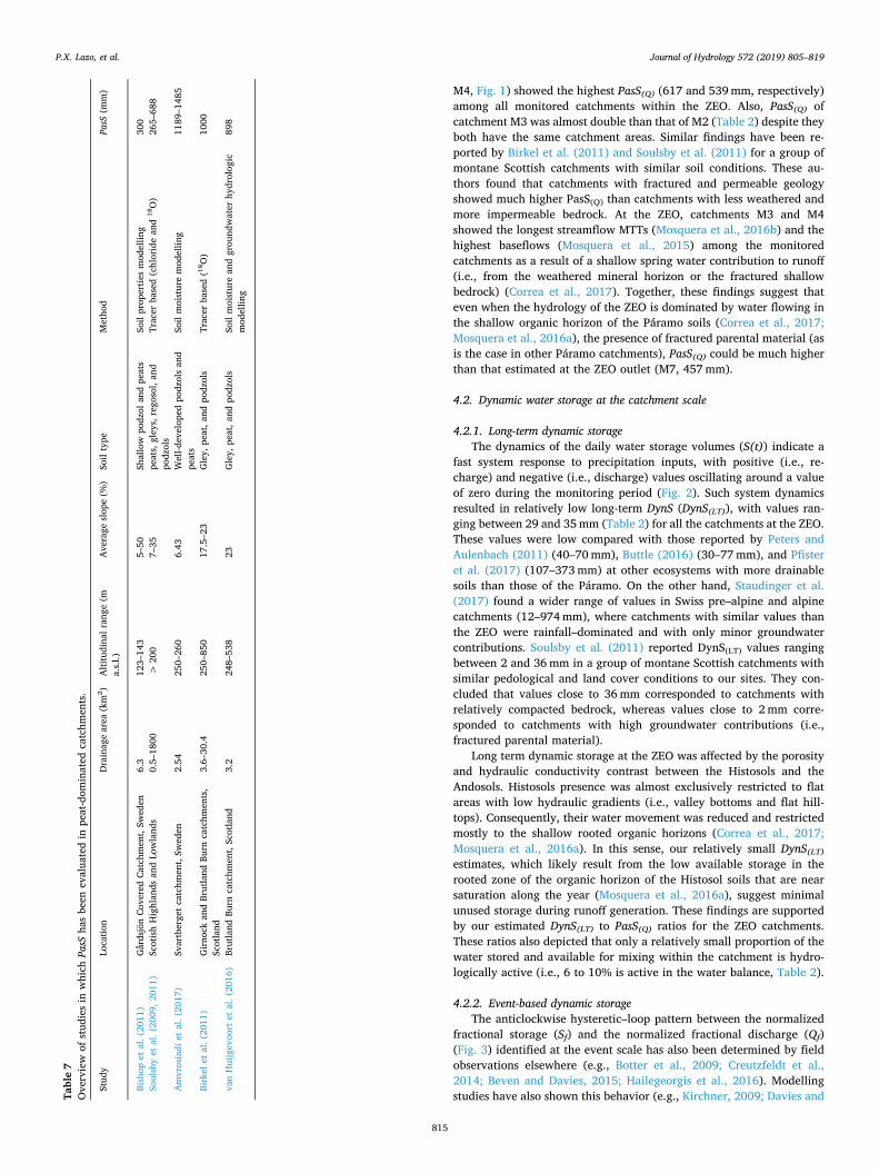
4.1.2. Passive storage estimation in relation to other catchmentsA summary of the studies in which PasS has been evaluated using

different calculation methods in peat-dominated catchments is shownin Table 7. Our estimated PasS(Q) values at the ZEO (313–617mm,Table 2) are similar to those reported by Bishop et al. (2011) via the

modelling of soil properties at the Gardsjön catchment in Sweden(300mm) and Soulsby et al. (2009, 2011) using TB methods in a groupof montane Scottish catchments (265–688mm). They attributed theserelatively small storage values to the retention of water in the relativelyshallow (<2m) peat type soils with little deeply sourced water con-tributions from groundwater storage. By contrast, our estimates are lowrelative to peat-dominated catchments in North Sweden estimatedusing soil moisture modelling (1189–1485mm) by Amvrosiadi et al.(2017). They are also low in relation to the values reported by Birkelet al. (2011) estimated via TB methods and van Huijgevoort et al.(2016) estimated using a TB distributed hydrological model for thepeat-dominated Girnock catchment in the Scottish highlands (1000 and898mm, respectively). Our values were also lower than those of non-peat-dominated catchments with different land covers (e.g., pasture,grasslands, and forests) in a gradient between the Swiss plateau andalpine regions (> 5000mm) reported by Staudinger et al. (2017). De-spite the differences in catchment features (e.g., precipitation season-ality, land cover, soil type and depth) among the study sites in-vestigated by these authors, they all attributed these high PasS(Q)estimates to water storage in deep groundwater reservoirs. That is, thehighly fractured and permeable parental material. At the ZEO, priorresearch has shown that water stored in the peat type Histosol soils (i.e.,wetlands) controls runoff generation (Correa et al., 2016; Mosqueraet al., 2015). In addition, other studies have also shown that wateroriginated from these wetlands is the main contributor to runoffyear–round and that deeply sourced groundwater contributions torunoff are minimal (Correa et al., 2017; Mosquera et al., 2016a). OurPasS(Q) estimates, similar to those in catchments with low groundwaterstorage availability and much lower than those in catchments withhighly fractured geology, evidence that these wetlands do not onlycontrol water production at the ZEO, but also the catchment’s waterstorage capacity.

4.1.3. How vegetation, soils, and precipitation control passive storage?Past research at the ZEO has shown the importance of the wetlands

(i.e., Histosols and cushion plants vegetation) on the catchments’ waterproduction (Correa et al., 2017, 2016; Mosquera et al., 2015). The highcorrelation between PasS(Q) and the wetlands cover in our nestedsystem of catchments (Table 6, Fig. 4) suggests that the wetlands alsoinfluence the catchments’ available storage for mixing. Similar hydro-logic dependence on wetlands storage has been reported at the ScottishHighlands (e.g., Birkel et al., 2011; Tetzlaff et al., 2014; Geris et al.,2015a,b, Geris et al., 2017). These findings also confirm that forcatchments with low groundwater contribution, the totality of PasS(Q)depends on their areal proportion of wetlands. Additionally, the strongcorrelation between PasS(Q) with the catchments’ mean annual dis-charge and runoff coefficients (R2 > 0.73, Table 6), further evidences

Fig. 3. a) Discharge hydrograph; b) temporal variability of the normalized fractional discharge (Qf) and storage (Sf) volumes; and c) rainfall amount during arepresentative rainfall–runoff event at the study site. The data correspond to an event monitored at the outlet of the basin (M7) on February 16th, 2012. The blackand grey lines correspond to the rising and recession limbs of the hydrograph, respectively. The red and green lines in subplot c) represent time during the rising andrecession limbs of the hydrograph in subplot a), respectively. (For interpretation of the references to colour in this figure legend, the reader is referred to the webversion of this article.)

Table 6Determination coefficients (R2) between the streamflow TB passive storage(PasS(Q)) of the catchments with landscape features and hydrologic variables.Values in bold represent significant correlations at a statistical level of 0.10(i.e., 90% confidence level).± values represents positive or negative correla-tions between variables, respectively. Qxx represents the flow rates, as fre-quency of non-exceedance, where xx shows the non-exceedance rate.

Variable name PasS(Q)

Hydrologic variables Dynamic Storage (mm) −0.20Passive Storage 1.00Mean Annual Precipitation −0.30Mean Annual Discharge 0.73Runoff Coefficient 0.75Qmin 0.24Q10 −0.18Q30 0.10Q50 0.13Q70 0.55Q90 0.67Qmax 0.03

Landscape features Area (km2) 0.61Slope (%) −0.45Andosols (% of total area) −0.56Histosols (% of total area) 0.51Tussock Grass (% of total area) −0.73Cushion plants (% of total area) 0.68Turi Formation (% of total area) 0.48Quaternary Deposits (% of total area) −0.28Quimsacocha Formation (% of total area) −0.05


813

how the wetlands storage influence runoff generation and regulation.Here, it is worth noting that even though wetlands cover only a rela-tively small proportion of the monitored catchment areas (i.e., 13–24%,Table 1), they control the catchments’ water production and storage atthe ZEO. These findings highlight the importance and the fragility ofriparian wetlands as the main – and in this particular case, the only –

water storage reservoir in ecosystems where the presence of peaty soil(i.e., Histosols) dominates.We also identified some PasS variations among the monitored

catchments worth highlighting. For instance, even though two of thesmaller headwater catchments M1 (0.20 km2) and M2 (0.38 km2) havesimilar areal proportions covered by wetlands (13–15%), the smallestcatchment M1 showed a much larger PasS(Q) than M2 (394mm versus313mm, respectively). In contrast, even though catchments M5(1.40 km2) and M6 (3.28 km2) also have similar wetland coverage(20–22%), they presented similar PasS(Q) (400–411mm). These ap-parent discrepancies likely result from differences in the catchments’average slopes as a metric of topography. For example, the steepesttopography of catchment M2 (24%) in relation to M1 (14%) is likely toexplain the lowest PasS(Q) of catchment M2. On the contrary, catch-ments M5 and M6 have similar slopes (18–20%, Table 1), factor thatseems to explain the similar amount of water stored by these catch-ments. Similar findings have been reported on Scottish peat-dominatedcatchments by Tetzlaff et al. (2014). These authors reported that lowgradient terrain produced poor drainage conditions, thus, ensuring highvolumes of water retained in peaty soils throughout the year whereassteeper terrain that enhances hydraulic gradients allows an enhancedwater movement, thus, reducing the amount of water stored in the soils.This combination of factors influencing the catchments’ PasS has alsobeen reported at other sites with different soil types (e.g., Sidle et al.,2001; Lehmann et al., 2007; Detty and McGuire, 2010; Soulsby et al.,2016). Overall, these findings evidence that that even though we didnot find a direct relationship between the catchments’ average slopesand their PasS(Q) via correlation analysis, catchments’ topography ex-erts controls in the amount of water available for internal mixing.It is also worth noting that two of the upper catchments (M3 and

Fig. 4. Relationships between the stream-flow TB passive storage (PasS(Q)) with a)cushion plants coverage, b) tussock grasscoverage, c) mean annual discharge, and d)runoff coefficient of the nested system ofcatchments. Vegetation is expressed as thepercentage of the areal extent of each ve-getation type to the total area of eachcatchment. Dashed lines represent the 5%and 95% confidence intervals of the re-lationships. Note: Given that water samplesused for the estimation of streamflow meantransit times were collected during baseflowconditions (Mosquera et al., 2016b), weexcluded data from catchments M3 and M4in the regression analysis to remove the ef-fect of contributions from a spring watersource to these small headwater catchments(Mosquera et al., 2015).

Fig. 5. Relationship between the event scale dynamic storage (DynS(ES)) andmaximum precipitation intensity during the runoff events (n= 42) at the outletof the basin, M7. Dashed lines represent the 5% and 95% confidence intervals ofthe relationship.


814

M4, Fig. 1) showed the highest PasS(Q) (617 and 539mm, respectively)among all monitored catchments within the ZEO. Also, PasS(Q) ofcatchment M3 was almost double than that of M2 (Table 2) despite theyboth have the same catchment areas. Similar findings have been re-ported by Birkel et al. (2011) and Soulsby et al. (2011) for a group ofmontane Scottish catchments with similar soil conditions. These au-thors found that catchments with fractured and permeable geologyshowed much higher PasS(Q) than catchments with less weathered andmore impermeable bedrock. At the ZEO, catchments M3 and M4showed the longest streamflow MTTs (Mosquera et al., 2016b) and thehighest baseflows (Mosquera et al., 2015) among the monitoredcatchments as a result of a shallow spring water contribution to runoff(i.e., from the weathered mineral horizon or the fractured shallowbedrock) (Correa et al., 2017). Together, these findings suggest thateven when the hydrology of the ZEO is dominated by water flowing inthe shallow organic horizon of the Páramo soils (Correa et al., 2017;Mosquera et al., 2016a), the presence of fractured parental material (asis the case in other Páramo catchments), PasS(Q) could be much higherthan that estimated at the ZEO outlet (M7, 457mm).

4.2. Dynamic water storage at the catchment scale

4.2.1. Long-term dynamic storageThe dynamics of the daily water storage volumes (S(t)) indicate a

fast system response to precipitation inputs, with positive (i.e., re-charge) and negative (i.e., discharge) values oscillating around a valueof zero during the monitoring period (Fig. 2). Such system dynamicsresulted in relatively low long-term DynS (DynS(LT)), with values ran-ging between 29 and 35mm (Table 2) for all the catchments at the ZEO.These values were low compared with those reported by Peters andAulenbach (2011) (40–70mm), Buttle (2016) (30–77mm), and Pfisteret al. (2017) (107–373mm) at other ecosystems with more drainablesoils than those of the Páramo. On the other hand, Staudinger et al.(2017) found a wider range of values in Swiss pre–alpine and alpinecatchments (12–974mm), where catchments with similar values thanthe ZEO were rainfall–dominated and with only minor groundwatercontributions. Soulsby et al. (2011) reported DynS(LT) values rangingbetween 2 and 36mm in a group of montane Scottish catchments withsimilar pedological and land cover conditions to our sites. They con-cluded that values close to 36mm corresponded to catchments withrelatively compacted bedrock, whereas values close to 2mm corre-sponded to catchments with high groundwater contributions (i.e.,fractured parental material).Long term dynamic storage at the ZEO was affected by the porosity

and hydraulic conductivity contrast between the Histosols and theAndosols. Histosols presence was almost exclusively restricted to flatareas with low hydraulic gradients (i.e., valley bottoms and flat hill-tops). Consequently, their water movement was reduced and restrictedmostly to the shallow rooted organic horizons (Correa et al., 2017;Mosquera et al., 2016a). In this sense, our relatively small DynS(LT)estimates, which likely result from the low available storage in therooted zone of the organic horizon of the Histosol soils that are nearsaturation along the year (Mosquera et al., 2016a), suggest minimalunused storage during runoff generation. These findings are supportedby our estimated DynS(LT) to PasS(Q) ratios for the ZEO catchments.These ratios also depicted that only a relatively small proportion of thewater stored and available for mixing within the catchment is hydro-logically active (i.e., 6 to 10% is active in the water balance, Table 2).

4.2.2. Event-based dynamic storageThe anticlockwise hysteretic–loop pattern between the normalized

fractional storage (Sf) and the normalized fractional discharge (Qf)(Fig. 3) identified at the event scale has also been determined by fieldobservations elsewhere (e.g., Botter et al., 2009; Creutzfeldt et al.,2014; Beven and Davies, 2015; Hailegeorgis et al., 2016). Modellingstudies have also shown this behavior (e.g., Kirchner, 2009; Davies andTa

ble7

Overviewofstudiesinwhich

PasShasbeenevaluatedinpeat-dominatedcatchments.

Study

Location

Drainagearea(km2 )

Altitudinalrange(m

a.s.l.)

Averageslope(%)Soiltype

Method

PasS(mm)

Bishopetal.(2011)

GårdsjönCoveredCatchment,Sweden

6.3

123–143

5–50

Shallowpodzolandpeats

Soilpropertiesmodelling

300

Soulsbyetal.(2009,2011)

ScotishHighlandsandLowlands

0.5–1800

>200

7–35

peats,gleys,regosol,and

podzols

Tracerbased(chlorideand18O)

265–688

Amvrosiadietal.(2017)

Svartbergetcatchment,Sweden

2.54

250–260

6.43

Well-developedpodzolsand

peats

Soilmoisturemodelling

1189–1485

Birkeletal.(2011)

GirnockandBrutlandBurncatchments,

Scotland

3.6–30.4

250–850

17.5–23

Gley,peat,andpodzols

Tracerbased(18 O)

1000

vanHuijgevoortetal.(2016)BrutlandBurncatchment,Scotland

3.2

248–538

23Gley,peat,andpodzols

Soilmoistureandgroundwaterhydrologic

modelling

898


815

Beven, 2015). The direction of the loop pattern has been shown todepend on different climatic, topographic, and parent material (Sproleset al., 2015). At the ZEO, the observed anticlockwise trend is likelyexplained by the combined effect of the Histosols (wetlands) high waterretention capacity and the year–round input of low intensity pre-cipitation. In other words, when water is added at the beginning of theevent, it quickly fills the available storage before ‘effective precipita-tion’ drives the runoff that is released to the streams. Then, afterantecedent moisture controlled storage threshold is reached (Mosqueraet al., 2016a), the soils begin releasing water to streams (black lines inFig. 3a and b). Once precipitation ceases, the moisture gained by thesoils allows for a sustained stormflow generation until the end of theevent (grey line in Fig. 3a and b), when the system returns to a stabilitycondition (i.e., Sf≈0) because of the high water retention capacity ofthe soils. These findings further explain the rapid changes in daily S(t)volumes (Fig. 2) and the flashy discharge response to precipitationpreviously reported at the ZEO (Mosquera et al., 2016b, 2015). Suchbehavior has also been reported by Fovet et al. (2015) in poorly drainedriparian zones at a headwater catchment in France. The consistentanticlockwise direction observed during all monitored events at allcatchments at ZEO further highlights the importance of the riparianHistosols in streamflow generation at the ZEO (Correa et al., 2017;Mosquera et al., 2016a).

4.2.3. How vegetation, soils, and precipitation control dynamic storage?In the long term, the range of variation of DynS(LT) among catch-

ments was very small (29–35mm). As a result, we could not attributetheir spatial variability to any particular catchment features or hydro-metric variables. On the other hand, at the event scale, DynS(ES) showedsignificant correlation with maximum P intensity (Fig. 5). This ob-servation suggests that the amount of hydraulically active water line-arly increases with rainfall intensity. This effect likely results from therapid filling of unsaturated pores in the shallow (30–40 cm) organichorizon of the Páramo soils, which then augment the connectivity ofsaturated soil patches as precipitation intensity and amount increases(Tromp-van Meerveld and McDonnell, 2006; Tetzlaff et al., 2014). Thiseffect causes a rapid activation of soil DynS, which in turn results in arapid delivery of water towards the stream network during rainfallevents.

4.3. A conceptual model of vegetation, soils, and precipitation controls onPáramo water storage

Our findings can be conceptualized in the context of the celerity ofthe hydraulic potentials (i.e., the propagation speed of a perturbationwithin the hydrologic system; McDonnell and Beven, 2014; Beven andDavies, 2015) in the Páramo soils and the tracer velocity through thehydrologic system. Combined hydrological behavior that influences thehydrological services provided by Páramo catchments. Fig. 6 showshow the rapid filling of available storage during rainfall events leads torapid streamflow response (i.e., the system celerity response). This re-sponse behavior, in combination with low evapotranspiration due tothe high year–round humidity (> 90%, Córdova et al., 2015), helpsmaintain the near saturated conditions of significant portions of thePáramo (i.e., the Histosol soils and wetlands). Thus, precipitationtranslates to runoff quickly via shallow subsurface flow in the first30–40 cm of the Páramo soils (Mosquera et al., 2016a) and this in turncontrols the water production capacity of Páramo catchments, as seenon the lefthand side of Fig. 6.The righthand side of Fig. 6 depicts the attenuation of the stable

isotopic composition in streamflow in relation to precipitation isotopiccomposition (Mosquera et al., 2016a) —which results from the rela-tively long time that water resides in the hydrologic system (Mosqueraet al., 2016b). The relatively high PasS values in the organic horizon ofthe soils at the ZEO shows that the velocity of the system is regulated bythe high water retention capacity of the Páramo wetlands. This

retention capacity is maintained by the year-round input of low in-tensity precipitation (Padrón et al., 2015). This combination of factorscontrol the water storage capacity, and thus, provide Páramo catch-ments with a high water regulation capacity (as shown on the righthandside of Fig. 6). As a result, when precipitation intensities increase, thesystem’s celerity perturbation is enhanced, and thus, a rapid response(minutes to hours) of DynS occurs. This effect occurs despite the effi-cient mixing of tracer in the larger available PasS of the wetlands soils(Mosquera et al., 2016a), which further reduces the velocity of thehydrologic system (weeks to months). This velocity reduction, in turn,increases the residence time of the isotopic tracer within the catch-ments. These findings highlight the vulnerability of Páramo catchmentsto changes in the temporal variability of precipitation and the potentialchanges in hydropedological conditions of the Páramo soils in responseto changes in land use and climate.For instance, this catchment hydrological behavior could be sig-

nificantly altered by the impact of common anthropic practices in thestudy region. Previous studies have shown that pine afforestation de-creased water yield and potato cultivation declined baseflow produc-tion in Páramo catchments (Buytaert et al., 2007). Similarly, affor-estation with pine plantations has shown to decline significantlyorganic carbon and the water retention capacity of Páramo soils (Farleyet al., 2004). These changes likely reflect a reduction in the MTT ofwater within the hydrologic system due to a significant reduction of thesystems’ passive storage. Effect that is likely to result in a reduction ofthe flow regulation capacity of Páramo catchments.Finally, it is worth highlighting the similarities of our catchment

storage findings in comparison to those in other regions of the world(e.g., the Scottish highlands; Birkel et al., 2011; Soulsby et al., 2009;Tetzlaff et al., 2015a; van Huijgevoort et al., 2016), despite differences

Fig. 6. Conceptual model of the factors influencing the Páramo water storage,hydrological dynamics, and ecosystem services provisioning.


816

in meteorological conditions. These similarities indicate that our find-ings can serve as a baseline for future water storage evaluations andcould be transferable to other peat-dominated ecosystems in the Andesand elsewhere.

5. Conclusions

Our catchment storage evaluation using a combination of hydro-metric, isotopic, and hydrophysical soil properties data yielded valu-able insights into the water passive and dynamic water storage of thePáramo. We demonstrated that streamflow mean transit time (MTT) isuseful for estimating catchment passive storage (PasS) and these esti-mates are comparable with hydrophysical soil properties and soil waterMTT based approaches. Together, these estimates provide a novel ap-proach to infer groundwater contributions to catchment storage. Wefound that the hydrologically active dynamic storage (DynS) corre-sponded to only a small proportion (6–10%) of the total PasS capacityof the Andean Páramo wetlands that contribute to runoff generation.Our findings also indicate that the DynS and water production capacityof the catchments is mainly controlled by rainfall intensity. In contrast,PasS and water regulation capacity is controlled mostly by the high-water retention capacity of the peaty soils (Histosols). These findingsprovide baseline information about the factors controlling the waterproduction and regulation ecosystem services provided by the Páramo.Future research should be targeted towards the investigation of theresilience of the Andean Páramo wetlands to sustain water productionand regulation in response to changes in environmental conditions dueto climate change and to better understand the role of hillslope soils(i.e., Andosols) in the provisioning of hydrological services in thePáramo and other high-elevation tropical environments.

Acknowledgments

This manuscript is an outcome of the MSc Program in Ecohydrologyof the University of Cuenca. We would like to thank INV Metals S.A.(Loma Larga Project) for the assistance in the logistics during the studyperiod. The authors also want to thank Irene Cardenas for her supportwith the laboratory analyses and Franklin Marin for his support withthe collection of soil samples for hydrophysical properties analyses. G.M. M. also thanks the support of the University of Cuenca’s DoctoralProgram in Water Resources. We also thank Editor Marco Borga,Conrado Tobón, and an anonymous reviewer for their valuable com-ments on earlier versions of this manuscript.

Funding

This research was funded by the Ecuadorian Secretary of HigherEducation, Science, Technology and Innovation (SENESCYT) in theframework of the project “Desarrollo de indicadores hidrológicos fun-cionales para la evaluación del impacto del cambio global en ecosis-temas Andinos”, and by the Central Research Office of the University ofCuenca (DIUC) in the framework of the project “Desarrollo de in-dicadores hidrológicos funcionales para evaluar la influencia de lasladeras y humedales en una cuenca de Páramo Húmedo”.

Conflict of interest

The authors declare no conflict of interest.

References

Allen, R., Pereira, L., Raes, D., Smith, M., 1998. Crop Evapotranspiration-Guidelines forComputing Crop Water Requirements-FAO Irrigation and Drainage Paper 56. FAO,Rome.

Amvrosiadi, N., Seibert, J., Grabs, T., Bishop, K., 2017. Water storage dynamics in a tillhillslope: the foundation for modeling flows and turnover times. Hydrol. Process. 31,4–14. https://doi.org/10.1002/hyp.11046.

Aparecido, L.M.T., Teodoro, G.S., Mosquera, G., Brum, M., Barros, F. de V., Pompeu, P.V.,Rodas, M., Lazo, P., Müller, C.S., Mulligan, M., Asbjornsen, H., Moore, G.W., Oliveira,R.S., 2018. Ecohydrological drivers of Neotropical vegetation in montane ecosystems.Ecohydrology e1932. https://doi.org/10.1002/eco.1932.

Asbjornsen, H., Manson, R.H., Scullion, J.J., Holwerda, F., Muñoz-Villers, L.E., Alvarado-Barrientos, M.S., Geissert, D., Dawson, T.E., McDonnell, J.J., Bruijnzeel, L.A., 2017.Interactions between payments for hydrologic services, landowner decisions, andecohydrological consequences: synergies and disconnection in the cloud forest zoneof central Veracruz, Mexico. Ecol. Soc. 22https://doi.org/10.5751/ES-09144-220225. art25.

Beven, K., Davies, J., 2015. Velocities, celerities and the basin of attraction in catchmentresponse. Hydrol. Process. 29, 5214–5226. https://doi.org/10.1002/hyp.10699.

Birkel, C., Soulsby, C., 2016. Linking tracers, water age and conceptual models to identifydominant runoff processes in a sparsely monitored humid tropical catchment. Hydrol.Process. 30, 4477–4493. https://doi.org/10.1002/hyp.10941.

Birkel, C., Soulsby, C., Tetzlaff, D., 2011. Modelling catchment-scale water storage dy-namics: reconciling dynamic storage with tracer-inferred passive storage. Hydrol.Process. 25, 3924–3936. https://doi.org/10.1002/hyp.8201.

Bishop, K., Seibert, J., Nyberg, L., Rodhe, A., 2011. Water storage in a till catchment. II:Implications of transmissivity feedback for flow paths and turnover times. Hydrol.Process. 25, 3950–3959. https://doi.org/10.1002/hyp.8355.

Boll, J., Selker, J.S., Nijssen, B.M., Steenhuis, T.S., Van Winkle, J., Jolles, E., 1991. Waterquality sampling under preferential flow conditions. In: Allen, R.G., Howell, T.A.,Pruitt, W.O., Walter, I.A., Jensen, M.E. (Eds.), Lysimeters for Evapotranspiration andEnvironmental Measurements. American Society of Civil Engineers, New York, pp.290–298.

Boll, J., Steenhuis, T.S., Selker, J.S., 1992. Fiberglass Wicks for Sampling of Water andSolutes in the Vadose Zone. Soil Sci. Soc. Am. J. 56, 701. https://doi.org/10.2136/sssaj1992.03615995005600030005x.

Botter, G., Porporato, A., Rodriguez-Iturbe, I., Rinaldo, A., 2009. Nonlinear storage-dis-charge relations and catchment streamflow regimes. Water Resour. Res. 45. https://doi.org/10.1029/2008WR007658.

Brauer, C.C., Teuling, A.J., Torfs, P.J.J.F., Uijlenhoet, R., 2013. Investigating storage-discharge relations in a lowland catchment using hydrograph fitting, recession ana-lysis, and soil moisture data. Water Resour. Res. 49, 4257–4264. https://doi.org/10.1002/wrcr.20320.

Brauman, K.A., Daily, G.C., Duarte, T.K., Mooney, H.A., 2007. The nature and value ofecosystem services: an overview highlighting hydrologic services. Annu. Rev.Environ. Resour. 32, 67–98. https://doi.org/10.1146/annurev.energy.32.031306.102758.

Buttle, J.M., 2016. Dynamic storage: a potential metric of inter-basin differences in sto-rage properties. Hydrol. Process. 30, 4644–4653. https://doi.org/10.1002/hyp.10931.

Buytaert, W., 2004. The Properties of the Soils of the South Ecuadorian Páramo and theImpact of Land Use Changes on their Hydrology. Katholieke Universiteit Leuven.

Buytaert, W., Beven, K., 2011. Models as multiple working hypotheses: hydrological si-mulation of tropical alpine wetlands. Hydrol. Process. 25, 1784–1799. https://doi.org/10.1002/hyp.7936.

Buytaert, W., Celleri, R., Willems, P., Bièvre, B. De, Wyseure, G., 2006. Spatial andtemporal rainfall variability in mountainous areas: a case study from the southEcuadorian Andes. J. Hydrol. 329, 413–421. https://doi.org/10.1016/J.JHYDROL.2006.02.031.

Buytaert, W., Iñiguez, V., Bièvre, B. De, 2007. The effects of afforestation and cultivationon water yield in the Andean páramo. For. Ecol. Manage. 251, 22–30. https://doi.org/10.1016/j.foreco.2007.06.035.

Coltorti, M., Ollier, C., 2000. Geomorphic and tectonic evolution of the EcuadorianAndes. Geomorphology 32, 1–19. https://doi.org/10.1016/S0169-555X(99)00036-7.

Córdova, M., Carrillo-Rojas, G., Crespo, P., Wilcox, B., Célleri, R., 2015. Evaluation of thePenman-Monteith (FAO 56 PM) method for calculating reference evapotranspirationusing limited data. Mt. Res. Dev. 35, 230–239. https://doi.org/10.1659/MRD-JOURNAL-D-14-0024.1.

Córdova, M., Célleri, R., Shellito, C.J., Orellana-Alvear, J., Abril, A., Carrillo-Rojas, G.,2016. Near-surface air temperature lapse rate over complex terrain in the southernEcuadorian andes: implications for temperature mapping. Arctic Antarct. Alp. Res.48, 673–684. https://doi.org/10.1657/AAAR0015-077.

Correa, A., Windhorst, D., Crespo, P., Célleri, R., Feyen, J., Breuer, L., 2016. Continuousversus event-based sampling: how many samples are required for deriving generalhydrological understanding on Ecuador’s páramo region? Hydrol. Process. 30,4059–4073. https://doi.org/10.1002/hyp.10975.

Correa, A., Windhorst, D., Tetzlaff, D., Crespo, P., Célleri, R., Feyen, J., Breuer, L., 2017.Temporal dynamics in dominant runoff sources and flow paths in the AndeanPáramo. Water Resour. Res. 53, 5998–6017. https://doi.org/10.1002/2016WR020187.

Cowie, R.M., Knowles, J.F., Dailey, K.R., Williams, M.W., Mills, T.J., Molotch, N.P., 2017.Sources of streamflow along a headwater catchment elevational gradient. J. Hydrol.https://doi.org/10.1016/j.jhydrol.2017.03.044.

Craig, H., 1961. Standard for reporting concentrations of deuterium and oxygen-18 innatural waters. Science 133, 1833–1834. https://doi.org/10.1126/science.133.3467.1833.

Crespo, P., Bücker, A., Feyen, J., Vaché, K.B., Frede, H.-G., Breuer, L., 2012. Preliminaryevaluation of the runoff processes in a remote montane cloud forest basin usingmixing model analysis and mean transit time. Hydrol. Process. 26, 3896–3910.https://doi.org/10.1002/hyp.8382.

Crespo, P.J., Feyen, J., Buytaert, W., Bücker, A., Breuer, L., Frede, H.-G., Ramírez, M.,2011. Identifying controls of the rainfall–runoff response of small catchments in thetropical Andes (Ecuador). J. Hydrol. 407, 164–174. https://doi.org/10.1016/j.


817

http://refhub.elsevier.com/S0022-1694(19)30246-X/h0005



https://doi.org/10.1002/hyp.11046

https://doi.org/10.1002/eco.1932

https://doi.org/10.5751/ES-09144-220225

https://doi.org/10.5751/ES-09144-220225










https://doi.org/10.2136/sssaj1992.03615995005600030005x


https://doi.org/10.1029/2008WR007658

https://doi.org/10.1029/2008WR007658

https://doi.org/10.1002/wrcr.20320

https://doi.org/10.1002/wrcr.20320

https://doi.org/10.1146/annurev.energy.32.031306.102758

https://doi.org/10.1146/annurev.energy.32.031306.102758







https://doi.org/10.1016/J.JHYDROL.2006.02.031

https://doi.org/10.1016/J.JHYDROL.2006.02.031

https://doi.org/10.1016/j.foreco.2007.06.035

https://doi.org/10.1016/j.foreco.2007.06.035

https://doi.org/10.1016/S0169-555X(99)00036-7

https://doi.org/10.1659/MRD-JOURNAL-D-14-0024.1

https://doi.org/10.1659/MRD-JOURNAL-D-14-0024.1

https://doi.org/10.1657/AAAR0015-077


https://doi.org/10.1002/2016WR020187

https://doi.org/10.1002/2016WR020187


https://doi.org/10.1126/science.133.3467.1833

https://doi.org/10.1126/science.133.3467.1833



jhydrol.2011.07.021.Creutzfeldt, B., Troch, P.A., Güntner, A., Ferré, T.P.A., Graeff, T., Merz, B., 2014. Storage-

discharge relationships at different catchment scales based on local high-precisiongravimetry. Hydrol. Process. 28, 1465–1475. https://doi.org/10.1002/hyp.9689.

Davies, J.A.C., Beven, K., 2015. Hysteresis and scale in catchment storage, flow andtransport. Hydrol. Process. 29, 3604–3615. https://doi.org/10.1002/hyp.10511.

Detty, J.M., McGuire, K.J., 2010. Threshold changes in storm runoff generation at a till-mantled headwater catchment. Water Resour. Res. 46. https://doi.org/10.1029/2009WR008102.

Dunkerley, D., 2008. Identifying individual rain events from pluviograph records: a re-view with analysis of data from an Australian dryland site. Hydrol. Process. 22,5024–5036. https://doi.org/10.1002/hyp.7122.

Dunn, S.M., Birkel, C., Tetzlaff, D., Soulsby, C., 2010. Transit time distributions of aconceptual model: their characteristics and sensitivities. Hydrol. Process. 24,1719–1729. https://doi.org/10.1002/hyp.7560.

FAO, 2009. Guidelines for Soil Description. Food and Agriculture Organization of theUnited Nations.

Farley, K.A., Kelly, E.F., Hofstede, R.G.M., 2004. Soil organic carbon and water retentionafter conversion of grasslands to pine plantations in the Ecuadorian Andes.Ecosystems 7, 729–739. https://doi.org/10.1007/s10021-004-0047-5.

Fischer, B.M.C., van Meerveld, H.J. (Ilja), Seibert, J., 2017. Spatial variability in theisotopic composition of rainfall in a small headwater catchment and its effect onhydrograph separation. J. Hydrol. 547, 755–769. https://doi.org/10.1016/j.jhydrol.2017.01.045.

Fovet, O., Ruiz, L., Hrachowitz, M., Faucheux, M., Gascuel-Odoux, C., 2015. Hydrologicalhysteresis and its value for assessing process consistency in catchment conceptualmodels. Hydrol. Earth Syst. Sci. 19, 105–123. https://doi.org/10.5194/hess-19-105-2015.

Geris, J., Tetzlaff, D., McDonnell, J., Soulsby, C., 2015a. The relative role of soil type andtree cover on water storage and transmission in northern headwater catchments.Hydrol. Process. 29, 1844–1860. https://doi.org/10.1002/hyp.10289.

Geris, J., Tetzlaff, D., McDonnell, J.J., Soulsby, C., 2017. Spatial and temporal patterns ofsoil water storage and vegetation water use in humid northern catchments. Sci. TotalEnviron. 595, 486–493. https://doi.org/10.1016/j.scitotenv.2017.03.275.

Geris, J., Tetzlaff, D., Soulsby, C., 2015b. Resistance and resilience to droughts: hydro-pedological controls on catchment storage and run-off response. Hydrol. Process. 29,4579–4593. https://doi.org/10.1002/hyp.10480.

Grant, L., Seyfried, M., McNamara, J., 2004. Spatial variation and temporal stability ofsoil water in a snow-dominated, mountain catchment. Hydrol. Process. 18,3493–3511. https://doi.org/10.1002/hyp.5798.

Guio Blanco, C.M., Brito Gomez, V.M., Crespo, P., Ließ, M., 2018. Spatial prediction ofsoil water retention in a Páramo landscape: methodological insight into machinelearning using random forest. Geoderma 316, 100–114. https://doi.org/10.1016/J.GEODERMA.2017.12.002.

Hailegeorgis, T.T., Alfredsen, K., Abdella, Y.S., Kolberg, S., 2016. Evaluation of stor-age–discharge relationships and recession analysis-based distributed hourly runoffsimulation in large-scale, mountainous and snow-influenced catchment. Hydrol. Sci.J. 61, 2872–2886. https://doi.org/10.1080/02626667.2016.1170939.

Hale, V.C., McDonnell, J.J., Stewart, M.K., Solomon, D.K., Doolitte, J., Ice, G.G., Pack,R.T., 2016. Effect of bedrock permeability on stream base flow mean transit timescaling relationships: 2. Process study of storage and release. Water Resour. Res. 52,1375–1397. https://doi.org/10.1002/2015WR017660.

Hamel, P., Riveros-Iregui, D., Ballari, D., Browning, T., Célleri, R., Chandler, D., Chun,K.P., Destouni, G., Jacobs, S., Jasechko, S., Johnson, M., Krishnaswamy, J., Poca, M.,Pompeu, P.V., Rocha, H., 2017. Watershed services in the humid tropics: opportu-nities from recent advances in ecohydrology. Ecohydrology. https://doi.org/10.1002/eco.1921. e1921.

Hasan, S., Troch, P.A., Bogaart, P.W., Kroner, C., 2008. Evaluating catchment-scale hy-drological modeling by means of terrestrial gravity observations. Water Resour. Res.44. https://doi.org/10.1029/2007WR006321.

Heidbüchel, I., Güntner, A., Blume, T., 2015. Use of cosmic ray neutron sensors for soilmoisture monitoring in forests. Hydrol. Earth Syst. Sci. Discuss. 12, 9813–9864.https://doi.org/10.5194/hessd-12-9813-2015.

Hofstede, R.G.M., Mena, V., Segarra, P., 2003. Los Paramos del Mundo.Holder, M.W., Brown, K.W., Thomas, J.C., Development of A Capillary Wick Unsaturated

Zone Pore Water Sampler, U.S. Environmental Protection Agency, Washington, D.C.,1989. Development of a Capillary Wick Unsaturated Zone Pore Water Sampler.Environmental Monitoring Systems Laboratory, Office of Research and Development,United States Environmental Protection Agency.

IAEA, 1997. Technical Procedure for Cumulative Monthly Sampling of Precipitation forIsotopic Analyses.

IUCN, 2002. High Andean Wetlands. Gland, Switzerland.IUSS Working Group WRB, 2015. World Reference Base for Soil Resources 2014, update

2015. International soil classification system for naming soils and creating legends forsoil maps. World Soil Resources Reports No. 106. FAO Rome.

Kirchner, J.W., 2009. Catchments as simple dynamical systems: catchment character-ization, rainfall-runoff modeling, and doing hydrology backward. Water Resour. Res.45, 1–34. https://doi.org/10.1029/2008WR006912.

Kirchner, J.W., Feng, X., Neal, C., 2000. Fractal stream chemistry and its implications forcontaminant transport in catchments. Nature 403, 524–527. https://doi.org/10.1038/35000537.

Knutson, J.H., Lee, S.B., Zhang, W.Q., Selker, J.S., 1993. Fiberglass wick preparation foruse in passive capillary wick soil pore-water samplers. Soil Sci. Soc. Am. J. 57, 1474.https://doi.org/10.2136/sssaj1993.03615995005700060013x.

Landon, M., Delin, G., Komor, S., Regan, C., 1999. Comparison of the stable-isotopiccomposition of soil water collected from suction lysimeters, wick samplers, and cores

in a sandy unsaturated zone. J. Hydrol. 224, 45–54. https://doi.org/10.1016/S0022-1694(99)00120-1.

Lehmann, P., Hinz, C., McGrath, G., Tromp-van Meerveld, H.J., McDonnell, J.J., 2007.Rainfall threshold for hillslope outflow: an emergent property of flow pathwayconnectivity. Hydrol. Earth Syst. Sci. 11, 1047–1063. https://doi.org/10.5194/hess-11-1047-2007.

Maloszewski, P., Zuber, A., 1996. Lumped parameter models for the interpretation ofenvironmental tracer data. In: Manual on Mathematical Models in IsotopeHydrogeology. TECDOC-910.

Małoszewski, P., Zuber, A., 1982. Determining the turnover time of groundwater systemswith the aid of environmental tracers. J. Hydrol. 57, 207–231. https://doi.org/10.1016/0022-1694(82)90147-0.

McDonnell, J.J., Beven, K., 2014. Debates-The future of hydrological sciences: a(common) path forward? a call to action aimed at understanding velocities, celeritiesand residence time distributions of the headwater hydrograph. Water Resour. Res. 50,5342–5350. https://doi.org/10.1002/2013WR015141.

McGuire, K.J., McDonnell, J.J., 2006. A review and evaluation of catchment transit timemodeling. J. Hydrol. 330, 543–563. https://doi.org/10.1016/j.jhydrol.2006.04.020.

McGuire, K.J., McDonnell, J.J., Weiler, M., Kendall, C., McGlynn, B.L., Welker, J.M.,Seibert, J., 2005. The role of topography on catchment-scale water residence time.Water Resour. Res. 41, n/a-n/a. https://doi.org/10.1029/2004WR003657.

Mcnamara, J.P., Tetzlaff, D., Bishop, K., Soulsby, C., Seyfried, M., Peters, N.E., Aulenbach,B.T., Hooper, R., 2011. Storage as a metric of catchment comparison. Hydrol. Process.25, 3364–3371. https://doi.org/10.1002/hyp.8113.

Moore, R.B., 2004. Introduction to salt dilution gauging for streamflow measurement Part2: constant-rate injection. Streamline Watershed Manag. Blull. 8, 11–15.

Mosquera, G.M., Célleri, R., Lazo, P.X., Vaché, K.B., Perakis, S.S., Crespo, P., 2016a.Combined use of isotopic and hydrometric data to conceptualize ecohydrologicalprocesses in a high-elevation tropical ecosystem. Hydrol. Process. 30, 2930–2947.https://doi.org/10.1002/hyp.10927.

Mosquera, G.M., Lazo, P.X., Célleri, R., Wilcox, B.P., Crespo, P., 2015. Runoff from tro-pical alpine grasslands increases with areal extent of wetlands. CATENA 125,120–128. https://doi.org/10.1016/j.catena.2014.10.010.

Mosquera, G.M., Segura, C., Vaché, K.B., Windhorst, D., Breuer, L., Crespo, P., 2016b.Insights into the water mean transit time in a high-elevation tropical ecosystem.Hydrol. Earth Syst. Sci. 20, 2987–3004. https://doi.org/10.5194/hess-20-2987-2016.

Nippgen, F., McGlynn, B.L., Emanuel, R.E., 2015. The spatial and temporal evolution ofcontributing areas. Water Resour. Res. 51, 4550–4573. https://doi.org/10.1002/2014WR016719.

Padrón, R.S., Wilcox, B.P., Crespo, P., Célleri, R., 2015. Rainfall in the Andean Páramo:new insights from high-resolution monitoring in Southern Ecuador. J.Hydrometeorol. 16, 985–996. https://doi.org/10.1175/JHM-D-14-0135.1.

Pearce, A.J., Stewart, M.K., Sklash, M.G., 1986. Storm runoff generation in humidheadwater catchments: 1. Where does the water come from? Water Resour. Res. 22,1263–1272. https://doi.org/10.1029/WR022i008p01263.

Penna, D., Stenni, B., Šanda, M., Wrede, S., Bogaard, T.A., Michelini, M., Fischer, B.M.C.,Gobbi, A., Mantese, N., Zuecco, G., Borga, M., Bonazza, M., Sobotková, M., Čejková,B., Wassenaar, L.I., 2012. Technical note: evaluation of between-sample memoryeffects in the analysis of δ2H and δ18O of water samples measured by laser spec-troscopes. Hydrol. Earth Syst. Sci. 16, 3925–3933. https://doi.org/10.5194/hess-16-3925-2012.

Peters, N.E., Aulenbach, B.T., 2011. Water storage at the Panola Mountain ResearchWatershed, Georgia, USA. Hydrol. Process. 25, 3878–3889. https://doi.org/10.1002/hyp.8334.

Pfister, L., Martínez-Carreras, N., Hissler, C., Klaus, J., Carrer, G.E., Stewart, M.K.,McDonnell, J.J., 2017. Bedrock geology controls on catchment storage, mixing, andrelease: a comparative analysis of 16 nested catchments. Hydrol. Process. 31,1828–1845. https://doi.org/10.1002/hyp.11134.

Picarro, 2010. ChemCorrect TM-Solving the Problem of Chemical Contaminants in H20Stable Isotope Research, PICARRO INC, California, USA.

Polk, M.H., Young, K.R., Baraer, M., Mark, B.G., McKenzie, J.M., Bury, J., Carey, M.,2017. Exploring hydrologic connections between tropical mountain wetlands andglacier recession in Peru’s Cordillera Blanca. Appl. Geogr. 78, 94–103. https://doi.org/10.1016/j.apgeog.2016.11.004.

Poulenard, J., Podwojewski, P., Herbillon, A.J., 2003. Characteristics of non-allophanicAndisols with hydric properties from the Ecuadorian páramos. Geoderma 117,267–281. https://doi.org/10.1016/S0016-7061(03)00128-9.

Quichimbo, P., Tenorio, G., Borja, P., Cárdenas, I., Crespo, P., Célleri, R., 2012. Efectossobre las propiedades físicas y químicas de los suelos por el cambio de la coberturavegetal y uso del suelo: Páramo de Quimsacocha al sur del Ecuador. SuelosEcuatoriales 42, 138–153.

Roa-García, M.C., Weiler, M., 2010. Integrated response and transit time distributions ofwatersheds by combining hydrograph separation and long-term transit time mod-eling. Hydrol. Earth Syst. Sci. 14, 1537–1549. https://doi.org/10.5194/hess-14-1537-2010.

Rosenberg, E.A., Clark, E.A., Steinemann, A.C., Lettenmaier, D.P., 2012. On the con-tribution of groundwater storage to interannual streamflow anomalies in theColorado River basin. Hydrol. Earth Syst. Sci. Discuss. 9, 13191–13230. https://doi.org/10.5194/hessd-9-13191-2012.

Safeeq, M., Hunsaker, C.T., 2016. Characterizing runoff and water yield for headwatercatchments in the Southern Sierra Nevada. JAWRA J. Am. Water Resour. Assoc. 52,1327–1346. https://doi.org/10.1111/1752-1688.12457.

Sayama, T., McDonnell, J.J., 2009. A new time-space accounting scheme to predictstream water residence time and hydrograph source components at the watershedscale. Water Resour. Res. 45, W07401. https://doi.org/10.1029/2008WR007549.

Sayama, T., McDonnell, J.J., Dhakal, A., Sullivan, K., 2011. How much water can a


818




https://doi.org/10.1029/2009WR008102

https://doi.org/10.1029/2009WR008102





https://doi.org/10.1007/s10021-004-0047-5



https://doi.org/10.5194/hess-19-105-2015



https://doi.org/10.1016/j.scitotenv.2017.03.275



https://doi.org/10.1016/J.GEODERMA.2017.12.002

https://doi.org/10.1016/J.GEODERMA.2017.12.002

https://doi.org/10.1080/02626667.2016.1170939

https://doi.org/10.1002/2015WR017660



https://doi.org/10.1029/2007WR006321

https://doi.org/10.5194/hessd-12-9813-2015






https://doi.org/10.1029/2008WR006912

https://doi.org/10.1038/35000537

https://doi.org/10.1038/35000537


https://doi.org/10.1016/S0022-1694(99)00120-1

https://doi.org/10.1016/S0022-1694(99)00120-1



https://doi.org/10.1016/0022-1694(82)90147-0

https://doi.org/10.1016/0022-1694(82)90147-0

https://doi.org/10.1002/2013WR015141


https://doi.org/10.1029/2004WR003657





https://doi.org/10.1016/j.catena.2014.10.010


https://doi.org/10.1002/2014WR016719

https://doi.org/10.1002/2014WR016719

https://doi.org/10.1175/JHM-D-14-0135.1

https://doi.org/10.1029/WR022i008p01263






https://doi.org/10.1016/j.apgeog.2016.11.004

https://doi.org/10.1016/j.apgeog.2016.11.004

https://doi.org/10.1016/S0016-7061(03)00128-9









https://doi.org/10.1111/1752-1688.12457

https://doi.org/10.1029/2008WR007549

watershed store? Hydrol. Process. 25, 3899–3908. https://doi.org/10.1002/hyp.8288.

Schoeneberger, P.J., Wysocki, D.A., Benham, E.C., Staff, S.S., 2012. Field Book forDescribing and Sampling Soils, Version 3.0. National Soil Survey Center, Lincoln, NE.

Seminario, S., 2016. Incertidumbre en la Precipitación Espacial Diaria Causada por redesPluviográficas Dispersas en una Microcuenca de Páramo densamente Monitoreada.Universidad de Cuenca.

Seyfried, M.S., Grant, L.E., Marks, D., Winstral, A., McNamara, J., 2009. Simulated soilwater storage effects on streamflow generation in a mountainous snowmelt en-vironment, Idaho, USA. Hydrol. Process. 23, 858–873. https://doi.org/10.1002/hyp.7211.

Sidle, R.C., Noguchi, S., Tsuboyama, Y., Laursen, K., 2001. A conceptual model of pre-ferential flow systems in forested hillslopes: evidence of self-organization. Hydrol.Process. 15, 1675–1692. https://doi.org/10.1002/hyp.233.

Sidle, R.C., Tsuboyama, Y., Noguchi, S., Hosoda, I., Fujieda, M., Shimizu, T., 1995.Seasonal hydrologic response at various spatial scales in a small forested catchment,Hitachi Ohta. Japan. J. Hydrol. 168, 227–250. https://doi.org/10.1016/0022-1694(94)02639-S.

Smakhtin, V., 2001. Low flow hydrology: a review. J. Hydrol. 240, 147–186. https://doi.org/10.1016/S0022-1694(00)00340-1.

Soulsby, C., Birkel, C., Geris, J., Dick, J., Tunaley, C., Tetzlaff, D., 2015. Stream water agedistributions controlled by storage dynamics and nonlinear hydrologic connectivity:modeling with high-resolution isotope data. Water Resour. Res. 51, 7759–7776.https://doi.org/10.1002/2015WR017888.

Soulsby, C., Birkel, C., Tetzlaff, D., 2016. Modelling storage-driven connectivity betweenlandscapes and riverscapes: towards a simple framework for long-term ecohy-drological assessment. Hydrol. Process. 30, 2482–2497. https://doi.org/10.1002/hyp.10862.

Soulsby, C., Neal, C., Laudon, H., Burns, D.A., Merot, P., Bonell, M., Dunn, S.M., Tetzlaff,D., 2008. Catchment data for process conceptualization: simply not enough? Hydrol.Process. 22, 2057–2061. https://doi.org/10.1002/hyp.7068.

Soulsby, C., Piegat, K., Seibert, J., Tetzlaff, D., 2011. Catchment-scale estimates of flowpath partitioning and water storage based on transit time and runoff modelling.Hydrol. Process. 25, 3960–3976. https://doi.org/10.1002/hyp.8324.

Soulsby, C., Tetzlaff, D., 2008. Towards simple approaches for mean residence time es-timation in ungauged basins using tracers and soil distributions. J. Hydrol. 363,60–74. https://doi.org/10.1016/j.jhydrol.2008.10.001.

Soulsby, C., Tetzlaff, D., Hrachowitz, M., 2009. Tracers and transit times: windows forviewing catchment scale storage? Hydrol. Process. 23, 3503–3507. https://doi.org/10.1002/hyp.7501.

Spence, C., 2007. On the relation between dynamic storage and runoff: a discussion onthresholds, efficiency, and function. Water Resour. Res. 43, n/a-n/a. https://doi.org/10.1029/2006WR005645.

Spence, C., Guan, X.J., Phillips, R., 2011. The Hydrological Functions of a Boreal Wetland.Wetlands 31, 75–85. https://doi.org/10.1007/s13157-010-0123-x.

Sproles, E.A., Leibowitz, S.G., Reager, J.T., Wigington, P.J., Famiglietti, J.S., Patil, S.D.,2015. GRACE storage-runoff hystereses reveal the dynamics of regional watersheds.Hydrol. Earth Syst. Sci. 19, 3253–3272. https://doi.org/10.5194/hess-19-3253-2015.

Staudinger, M., Stoelzle, M., Seeger, S., Seibert, J., Weiler, M., Stahl, K., 2017. Catchmentwater storage variation with elevation. Hydrol. Process. 31, 2000–2015. https://doi.org/10.1002/hyp.11158.

Sucozhañay, A., Célleri, R., 2018. Impact of rain gauges distribution on the runoff si-mulation of a small mountain catchment in Southern Ecuador. Water 10, 1169.https://doi.org/10.3390/w10091169.

Sun, G., Hallema, D., Asbjornsen, H., 2017. Ecohydrological processes and ecosystemservices in the Anthropocene: a review. Ecol. Process. 6, 35. https://doi.org/10.1186/s13717-017-0104-6.

Tetzlaff, D., Birkel, C., Dick, J., Geris, J., Soulsby, C., 2014. Storage dynamics in hydro-pedological units control hillslope connectivity, runoff generation, and the evolutionof catchment transit time distributions. Water Resour. Res. 50, 969–985. https://doi.org/10.1002/2013WR014147.

Tetzlaff, D., Buttle, J., Carey, S.K., McGuire, K., Laudon, H., Soulsby, C., 2015a. Tracer-based assessment of flow paths, storage and runoff generation in northern catch-ments: a review. Hydrol. Process. 29, 3475–3490. https://doi.org/10.1002/hyp.10412.

Tetzlaff, D., Buttle, J., Carey, S.K., van Huijgevoort, M.H.J., Laudon, H., McNamara, J.P.,Mitchell, C.P.J., Spence, C., Gabor, R.S., Soulsby, C., 2015b. A preliminary assess-ment of water partitioning and ecohydrological coupling in northern headwatersusing stable isotopes and conceptual runoff models. Hydrol. Process. 29, 5153–5173.https://doi.org/10.1002/hyp.10515.

Tromp-van Meerveld, H.J., McDonnell, J.J., 2006. Threshold relations in subsurfacestormflow: 2. The fill and spill hypothesis. Water Resour. Res. 42. https://doi.org/10.1029/2004WR003800.

U.S. Bureau of Reclamation, 2001. Water Measurement Manual. Washington DC.USDA, NRCS, 2004. Soil Survey Laboratory Methods Manual: Soil Survey Investigations

Report No. 42, Version 4.0, November 2004. United States Department of AgricultureNatural Resources Conservation Service.

van Huijgevoort, M.H.J., Tetzlaff, D., Sutanudjaja, E.H., Soulsby, C., 2016. Using highresolution tracer data to constrain water storage, flux and age estimates in a spatiallydistributed rainfall-runoff model. Hydrol. Process. 30, 4761–4778. https://doi.org/10.1002/hyp.10902.

Viviroli, D., Dürr, H.H., Messerli, B., Meybeck, M., Weingartner, R., 2007. Mountains ofthe world, water towers for humanity: typology, mapping, and global significance.Water Resour. Res. 43. https://doi.org/10.1029/2006WR005653.

Weiler, M., McGlynn, B.L., McGuire, K.J., McDonnell, J.J., 2003. How does rainfall be-come runoff? a combined tracer and runoff transfer function approach. Water Resour.Res. 39, n/a-n/a. https://doi.org/10.1029/2003WR002331.

Wright, C., Kagawa-Viviani, A., Gerlein-Safdi, C., Mosquera, G.M., Poca, M., Tseng, H.,Chun, K.P., 2017. Advancing ecohydrology in the changing tropics: perspectives fromearly career scientists. Ecohydrology e1918. https://doi.org/10.1002/eco.1918.


819











https://doi.org/10.1016/0022-1694(94)02639-S

https://doi.org/10.1016/0022-1694(94)02639-S

https://doi.org/10.1016/S0022-1694(00)00340-1

https://doi.org/10.1016/S0022-1694(00)00340-1

https://doi.org/10.1002/2015WR017888








https://doi.org/10.1029/2006WR005645

https://doi.org/10.1029/2006WR005645

https://doi.org/10.1007/s13157-010-0123-x




https://doi.org/10.3390/w10091169

https://doi.org/10.1186/s13717-017-0104-6

https://doi.org/10.1186/s13717-017-0104-6

https://doi.org/10.1002/2013WR014147

https://doi.org/10.1002/2013WR014147




https://doi.org/10.1029/2004WR003800

https://doi.org/10.1029/2004WR003800



https://doi.org/10.1029/2006WR005653

https://doi.org/10.1029/2003WR002331


The role of vegetation, soils, and precipitation on water ...

Documents

Transcript of The role of vegetation, soils, and precipitation on water ...