THE ROLE OF SNAP AND HABIT FORMATION ON HOUSEHOLD ...

University of Kentucky University of Kentucky

UKnowledge UKnowledge

Theses and Dissertations--Agricultural Economics Agricultural Economics

2017

THE ROLE OF SNAP AND HABIT FORMATION ON HOUSEHOLD THE ROLE OF SNAP AND HABIT FORMATION ON HOUSEHOLD

CONSUMPTION BEHAVIOR CONSUMPTION BEHAVIOR

Shaheer Burney University of Kentucky, [email protected] Digital Object Identifier: https://doi.org/10.13023/ETD.2017.220

Right click to open a feedback form in a new tab to let us know how this document benefits you. Right click to open a feedback form in a new tab to let us know how this document benefits you.

Recommended Citation Recommended Citation Burney, Shaheer, "THE ROLE OF SNAP AND HABIT FORMATION ON HOUSEHOLD CONSUMPTION BEHAVIOR" (2017). Theses and Dissertations--Agricultural Economics. 56. https://uknowledge.uky.edu/agecon_etds/56

This Doctoral Dissertation is brought to you for free and open access by the Agricultural Economics at UKnowledge. It has been accepted for inclusion in Theses and Dissertations--Agricultural Economics by an authorized administrator of UKnowledge. For more information, please contact [email protected].

http://uknowledge.uky.edu/

http://uknowledge.uky.edu/

https://uknowledge.uky.edu/

https://uknowledge.uky.edu/agecon_etds

https://uknowledge.uky.edu/agecon_etds

https://uknowledge.uky.edu/agecon

https://uky.az1.qualtrics.com/jfe/form/SV_9mq8fx2GnONRfz7

mailto:[email protected]

STUDENT AGREEMENT: STUDENT AGREEMENT:

I represent that my thesis or dissertation and abstract are my original work. Proper attribution

has been given to all outside sources. I understand that I am solely responsible for obtaining

any needed copyright permissions. I have obtained needed written permission statement(s)

from the owner(s) of each third-party copyrighted matter to be included in my work, allowing

electronic distribution (if such use is not permitted by the fair use doctrine) which will be

submitted to UKnowledge as Additional File.

I hereby grant to The University of Kentucky and its agents the irrevocable, non-exclusive, and

royalty-free license to archive and make accessible my work in whole or in part in all forms of

media, now or hereafter known. I agree that the document mentioned above may be made

available immediately for worldwide access unless an embargo applies.

I retain all other ownership rights to the copyright of my work. I also retain the right to use in

future works (such as articles or books) all or part of my work. I understand that I am free to

register the copyright to my work.

REVIEW, APPROVAL AND ACCEPTANCE REVIEW, APPROVAL AND ACCEPTANCE

The document mentioned above has been reviewed and accepted by the student’s advisor, on

behalf of the advisory committee, and by the Director of Graduate Studies (DGS), on behalf of

the program; we verify that this is the final, approved version of the student’s thesis including all

changes required by the advisory committee. The undersigned agree to abide by the statements

above.

Shaheer Burney, Student

Dr. Alison F. Davis, Major Professor

Dr. Carl R. Dillon, Director of Graduate Studies

THE ROLE OF SNAP AND HABIT FORMATION

ON HOUSEHOLD CONSUMPTION BEHAVIOR

_____________________________

DISSERTATION

_____________________________

A dissertation submitted in partial fulfillment of the

requirements for the degree of Doctor of Philosophy in the

College of Agriculture, Food and Environment

at the University of Kentucky

By

Shaheer Burney

Lexington, Kentucky

Director: Dr. Alison F. Davis, Professor of Agricultural Economics

Lexington, Kentucky

2017

Copyright © Shaheer Burney 2017

ABSTRACT OF DISSERTATION



This collection of essays examines the impact of two antecedents of household

food consumption: SNAP and habit formation to nutrients. Household food choice

invariably plays a substantial role in health outcomes such as obesity. Low-income

households may be especially vulnerable to obesity as they face a more restricted set of

food choices due to income constraints and may have less information on healthy eating

relative to high-income households. This dissertation unravels this dynamic by providing

causal estimates of the effect of two major determinants of food choice.

Chapter 2 and chapter 3 test the impact of SNAP participation on consumption of

foods that are likely to cause obesity. With some exceptions, SNAP restricts benefits to

be spent only on unprepared grocery food items from participating retailers. Chapter 2

considers the broad category of Food Away From Home (FAFH) which is shown to be

less healthy than meals prepared at home and shows that SNAP significantly reduces

FAFH expenditure of participants. However, the magnitude of this decrease is not large

enough to have a tangible impact on obesity. Chapter 3 considers household expenditure

on carbonated soda, which is the key source of sugar intake among low-income

households. Not only is carbonated soda SNAP-eligible, it is cheaper when purchased

with SNAP benefits relative to cash because benefits are exempt from all sales taxes.

Results show that SNAP participation leads to a significant rise in carbonated soda sales

in low-income counties. I also find that the SNAP tax exemption does not lead to higher

consumption among participants relative to non-participants.

Chapter 4 tests habit formation to dietary fat using purchases of ground meat and

milk products. Products in both categories have salient fat content information on the

packaging. Products within each category differ only by fat content and are usually

identical otherwise. Differences in habit formation are, therefore, caused by different

levels of fat content. Results show a positive association between habit formation and fat

content for all products in the ground meat category and all products, except fat-free

milk, in the milk category. However, this relationship is modest leading to the conclusion

that policy interventions, such as a saturated fat tax, might be effective in discouraging

consumption of high fat products.

KEYWORDS: SNAP, Consumer Behavior, Habit Formation,

FAFH, Demand System, Carbonated Soda

______________________________

______________________________

Shaheer Burney

June 4, 2017



By

Shaheer Burney

______________________________

Director of Dissertation

______________________________

Director of Graduate Studies

______________________________

Dr. Alison F. Davis

Dr. Carl R. Dillon

June 4, 2017

To my parents, Tanveer and Samina Burney, for their love, encouragement, and sacrifice.

Without their exemplary support, none of my successes in life would have been possible.

iii

ACKNOWLEDGMENTS

I would like to acknowledge the continual support provided by my advisor and

Dissertation Chair, Dr. Alison Davis, who gave me the opportunity to pursue my interests

and encouraged me to become an independent researcher. With her support, I was able to

develop the skills essential for rigorous academic research. Next, I would like to

acknowledge the contribution of my Dissertation Committee members, Dr. Yuqing

Zheng and Dr. Steven Buck. I thank Dr. Zheng for providing undeterred mentorship

throughout the dissertation process and for giving me the confidence to follow ambitious

ideas. I thank Dr. Steven Buck for investing his time and effort in teaching me the

intricacies of research and helping me polish my dissertation essays. I would also like to

acknowledge the rest of the Dissertation Committee, and outside reader, respectively: Dr.

David Freshwater, Dr. Aaron Yelowitz, and Dr. Gregg Rentfrow. Each member provided

invaluable feedback that imparted cogency to the analysis and improved the overall

dissertation in many important ways.

In addition, I would like to thank my parents, Tanveer and Samina Burney, for

teaching me the value of scholarship and hard work. Without the upbringing I was

afforded, I would not have the curiosity or the courage to ask difficult questions that

invariably led to the composition of these essays. Finally, I acknowledge the contribution

of my friends and confidantes who gave me an avenue for intellectual discourse and a

fulfilling reprieve when I needed it.

iv

TABLE OF CONTENTS

ACKNOWLEDGMENTS ................................................................................................. iii

LIST OF TABLES ............................................................................................................. vi

LIST OF FIGURES .......................................................................................................... vii

CHAPTER 1: INTRODUCTION ....................................................................................... 1

CHAPTER 2: HOUSEHOLD CONSUMPTION RESPONSES TO SNAP

PARTICIPATION .............................................................................................................. 6

I. Introduction .............................................................................................................. 7

II. Background ............................................................................................................ 10

III. Data .................................................................................................................... 12

IV. Descriptive Analysis .......................................................................................... 13

A. Treatment and Control Groups ........................................................................... 14

B. The Effect of the Recession ............................................................................... 16

V. Research Design and Methodology ....................................................................... 18

A. The Effect of Income.......................................................................................... 21

VI. Results ................................................................................................................ 22

VII. Discussion .......................................................................................................... 26

VIII. Conclusion .......................................................................................................... 28

IX. Tables ................................................................................................................. 30

X. Figures................................................................................................................ 38

CHAPTER 3: THE IMPACT OF SNAP PARTICIPATION ON SALES OF

CARBONATED SODA ................................................................................................... 43

I. Introduction ............................................................................................................ 44

II. Literature Review................................................................................................... 46

III. Research Design ................................................................................................. 47

A. Factor Analysis ................................................................................................... 47

B. Difference-In-Difference .................................................................................... 50

IV. Data .................................................................................................................... 52

V. Empirical Model .................................................................................................... 55

VI. Results and Discussion ....................................................................................... 56

A. Soda Tax ............................................................................................................. 60

VII. Conclusion .......................................................................................................... 62

VIII. Tables ................................................................................................................. 64

v

IX. Figures ................................................................................................................ 77

CHAPTER 4: HABIT FORMATION IN US DEMAND FOR DIETARY FAT ............ 82

I. Introduction ............................................................................................................ 83

II. Literature Review................................................................................................... 86

III. Conceptual Model .............................................................................................. 88

IV. Empirical Model ................................................................................................. 90

V. Data ........................................................................................................................ 92

VI. Results ................................................................................................................ 94

VII. Discussion .......................................................................................................... 96

VIII. Conclusion .......................................................................................................... 98

IX. Tables ................................................................................................................. 99

REFERENCES ............................................................................................................... 104

VITA ............................................................................................................................... 110

vi

LIST OF TABLES

Table 2-1. CPS Food Security Supplement Descriptive Statistics by Cohort .................. 30

Table 2-2. SNAP Participation Growth Rate by Cohort between 2000 and 2011 ............ 31

Table 2-3. OLS Regression on Weekly FAFH Share of Total Food ................................ 32

Table 2-4. OLS Regression on Weekly FAFH Expenditure and FAFH Share ................ 33

Table 2-5. OLS Regression on Weekly FAFH Share of Total Food (Full) ...................... 34

Table 2-6. OLS Regression on Weekly FAFH Expenditure and FAFH Share (Full) ...... 35

Table 2-7. OLS Regression on Weekly FAFH Expenditure and FAFH Share with Leads

and Lags .......................................................................................................... 36

Table 2-8. OLS Regression on Weekly FAFH Expenditure and FAFH Share by

Household Income .......................................................................................... 37

Table 3-1. State-Level Policy Option Descriptions .......................................................... 64

Table 3-2(a). Factor Analysis on State-Policy Options: Correlations .............................. 65

Table 3-2(b). Factor Analysis on State-Policy Options: Factor Loadings ........................ 66

Table 3-3. SNAP Participation Growth and Carbonated Soda Sales by Cohort, 2008 to

2012................................................................................................................. 67

Table 3-4. Summary Statistics by Cohort ......................................................................... 68

Table 3-5. Change in Average Weekly County-Level Soda Sales by Cohort .................. 69

Table 3-6. Difference In Difference Estimates on Weekly Carbonated Soda Sales ......... 70

Table 3-7. Difference In Difference Estimates on Weekly Carbonated Soda Sales (Full)71

Table 3-8. Difference In Difference Estimates on Log Per-Capita Sales of Carbonated

Soda................................................................................................................. 72

Table 3-9. Difference In Difference Model on Weekly Carbonated Soda Sales with Leads

and Lags (Base Level: 2006) .......................................................................... 73

Table 3-10. Difference In Difference Estimates on Weekly Carbonated Soda Sales with

Week Fixed Effects ......................................................................................... 74

Table 3-11. Average Weekly County-Level Change in Carbonated Soda Sales Relative to

SNAP Benefits ................................................................................................ 75

Table 3-12. Change in Average Weekly County-Level SNAP Benefits by Cohort ......... 76

Table 4-1. Average Monthly Expenditure and Quantity by Synthetic Household ........... 99

Table 4-2(a). Summary Statistics of Sample: Ground Meat Category ........................... 100

Table 4-2(b). Summary Statistics of Sample: Milk Category......................................... 101

Table 4-3. Habit Formation Parameter Estimates ........................................................... 102

Table 4-4. Long Run Unconditional Own and Cross-Price Elasticities ......................... 103

vii

LIST OF FIGURES

Figure 2-1: National Average SNAP Caseloads ............................................................... 38

Figure 2-2: Changes in SNAP Participation in High Growth and Low Growth Cohorts:

Index=2000 ..................................................................................................... 39

Figure 2-3: Annual Aggregate FAFH Expenditure .......................................................... 40

Figure 2-4: Average State Poverty Rate by Cohort, Index=2001 ..................................... 41

Figure 2-5: BBCE Adoption of High Growth and Low Growth States by Year .............. 42

Figure 3-1: Treatment and Control States by Index of Willingness, 2008, Factor 1 only 77

Figure 3-2: Treatment and Control States by Index of Willingness, 2008, Using Factor 1

and Factor 2..................................................................................................... 78

Figure 3-3: Combined State and Local Grocery Tax by County, 2014 ............................ 79

Figure 3-4: SNAP Participation by Cohort Indexed to 2008, 2006 to 2012 ..................... 80

Figure 3-5: Weekly Carbonated Soda Sales by Cohort Indexed to 2008, 2006 to 2015 .. 81

1

CHAPTER 1: INTRODUCTION

The Supplemental Nutrition Assistance Program (SNAP) (formerly known as the Food

Stamp Program) is the largest nutrition assistance program in the US. It provides in-kind

benefits to food insecure households based on a broadly defined eligibility criteria.

Relative to other nutrition assistance programs that target narrow demographics such as

The Special Supplemental Nutrition Program for Women, Infants, and Children (WIC),

which provides benefits for pregnant and nursing mothers and nutritionally at-risk infants

and children, SNAP caters to generally all low-income households. As a result, it is an

important safety net for impoverished families.

Over the last few decades, SNAP has gone through a series of drastic changes.

While initially meant to alleviate food insecurity, the program’s goals have expanded

towards encouraging beneficiaries to consume healthy diets. This two-pronged approach

has developed at the heels of a rapid surge in obesity rates among low-income households

in the US. Moreover, SNAP has seen a consistent increase in program caseloads across

the country since the early 2000s. In large part, this can be explained by state-level

adoption of policies that substantially eased the eligibility criteria and reduced

administrative burden. Some examples of these policies include the reduction of the asset

limit or complete elimination of the asset test, introduction of the Electronic Benefit

Transfer (EBT) system, extension of eligibility to non-citizen immigrants, and use of

online application systems. The concomitant spread of obesity and expansion of SNAP

have led some researchers to question the link between the two events.

2

Initiatives to promote healthy diets include an outright restriction on what

beneficiaries can spend SNAP dollars on. The program restricts purchases to include only

grocery food that requires at-home preparation for consumption. However, there are two

major caveats that compromise the efficacy of this initiative. First, most SNAP

participants have household food expenditure greater than the amount of benefits they

receive. These households, called “inframarginal” households, are easily able to

substitute current cash expenditure on food with SNAP benefits and utilize the now-

available cash to purchase products ineligible with SNAP benefits. The fungibility of

benefits with cash essentially renders the SNAP food restriction non-binding. Second, a

controversial exception to the SNAP food restriction is Sugar-Sweetened Beverages

(SSBs). It is well-established that SSBs, such as carbonated soda and sugar-sweetened

fruit juices, are one of the primary contributors to America’s obesity epidemic. Not only

are SSB products SNAP-eligible they are also exempt from all state and local sales taxes

when purchased with benefits. As a result, the extent to which SNAP achieves the

objective of encouraging low-income households to make healthy eating choices is a

question which has largely been unanswered.

An important factor that confounds our understanding of SNAP and its impacts on

consumption behavior is selection bias that arises from participation. That is, households

that choose to participate in the program may have unobservable differences from those

that are eligible but do not participate. Selection bias, if unaddressed, poses a serious

challenge to obtaining unbiased estimates and has led to lack of consensus on the effects

of SNAP on nutritional outcomes. Researchers have employed a series of methods to

3

overcome this issue, ranging from the use of instrumental variables to employing a

natural experiment for identification.

This collection of essays explores the multifaceted nature of the obesity epidemic

in the US. It spans the dynamic between household consumption behavior and

government welfare policies that are in place to combat obesity. While much research has

been devoted to analyzing the impact of these two antecedents, given the complex nature

of their mutual interdependence there is a growing need to study them concurrently. This

dissertation addresses this issue and provides insight into how public policy can be used

to drive behavior modification. One of the main contributions of this dissertation is the

use of innovative research design to provide causal estimates of the effect of SNAP on

consumption behavior. I utilize state-level variation in SNAP participation arising from

two major economic downturns in the US in the past two decades to circumvent the issue

of selection bias. The first two essays (Chapter 2 and 3) provide estimates obtained from

the application from this methodology. To the best of my knowledge, the use of

recessions as natural experiments in this context is unprecedented.

The main focus of the first essay (Chapter 2) is to determine the impact of SNAP

on obesity through the medium of Food Away From Home (FAFH) consumption. The

paradoxical positive association between food insecurity and obesity has led researchers

to identify FAFH expenditure as one of the possible causes of overweight among low-

income individuals. While FAFH does not qualify for purchase with SNAP dollars,

inframarginal households are able to circumvent this restriction. This study exploits

variation arising from the early 2000s recession to identify the impact of SNAP on

FAFH. Results show that SNAP has been largely successful in achieving its goal of

4

encouraging households to decrease FAFH expenditure. However, an informal

calculation shows that the FAFH decrease has a trivial effect on obesity.

The second essay (Chapter 3) explores the impact of SNAP participation on

consumption of carbonated soda. It is not surprising that the inclusion of carbonated soda

in the basket of SNAP-eligible products is widely debated given that carbonated soda is

one of the largest sources of sugar consumption in the country. This essay utilizes state-

level variation in SNAP participation arising from the Great Recession of 2008 to

identify the effect of SNAP on carbonated soda sales. Results show that SNAP does lead

to a non-trivial increase in weekly county-level soda sales but the tax exemption has little

to no influence on this relationship. As a result, policymakers need to carefully consider

whether imposing sales taxes on soda will produce a tangible decrease in soda

consumption. In addition, these taxes might be regressive as there is some evidence that

low-income households have a higher per-capita SSB consumption relative to high-

income households.

The third essay considers the possibility that habit formation might be an

impediment to behavior modification, thus subduing public efforts to encourage low-

income households to make healthy nutrition choices. This study delves into the

attributes of food to examine whether habit formation occurs at the nutrient level. I

estimate habit formation to dietary fat using purchases of two categories of products that

display salient fat content information on the packaging. I find that while these products

exhibit strong habit formation, there is only weak evidence for a positive relationship

between habit formation and fat content. These results have broad implications for

whether a tax on saturated fat is a viable policy option. A saturated fat tax may not lead to

5

substitution to lower-fat products, however, given the limited responsiveness of demand

to price changes it might be an effective tool for raising revenue.

The three essays in this dissertation provide insight into one of the most

penetrating issues of today. By many measures, obesity has reached epidemic

proportions. SNAP has been a major driving force behind preventing households from

falling into poverty and consequent food insecurity. Even though most beneficiaries are

considered inframarginal, participation does lead to greater expenditure on FAH relative

to FAFH. However, SNAP-eligible goods include SSBs which, consequently, leads

households to increase consumption of carbonated soda. Welfare programs need to be

designed such that they target the correct demographic and in an effective way. Poorly

designed programs, though well-intentioned, may exacerbate the prevalence of obesity.

Policy interventions such as Pigouvian taxes need to be considered concurrently with

welfare programs. As a result, public policy must be comprised of a menu of options that

target different aspects of household consumption behavior.

6

CHAPTER 2: HOUSEHOLD CONSUMPTION RESPONSES TO SNAP

PARTICIPATION

Obesity is inordinately prevalent among food insecure households in the US. Some

researchers have identified the consumption of unhealthy food a major source of this

seemingly paradoxical relationship. One of the goals of the Supplemental Nutrition

Assistance Program (SNAP), formerly known as the Food Stamp Program, is to

encourage healthy eating behavior among low-income households. However, literature

lacks conclusive evidence for the success of the program in achieving that goal. This

paper exploits an underutilized source of variation, the early-2000s recession in the US,

to determine the impact of SNAP participation on household Food Away From Home

(FAFH) expenditures. A Difference in Difference model is constructed using high post-

recession growth in SNAP caseloads as treatment. The results show that households in

the treatment cohort significantly decrease consumption of FAFH relative to households

in the control group. This provides evidence that SNAP participation leads households to

make healthier eating choices. However, reductions in FAFH are too small to have a

tangible impact on obesity.

7

I. Introduction

Supplemental Nutrition Assistance Program (SNAP) is a federal nutrition-assistance

program that is regulated by the Food and Nutrition Service (FNS) of the USDA and

provides welfare benefits to numerous households throughout the United States. While

the program has been touted for successfully targeting food insecurity in the US, it has

also been criticized for having the unintended consequence of promoting obesity in low

income households. The food insecurity-obesity paradox (Dietz, 1995), which states that

there is a positive association between the contradictory states of food insecurity and

obesity, has long puzzled researchers. Intuitively, households that are unable to fulfill the

nutrition needs of their members should exhibit starvation. However, in practice food

insecurity has been shown to be positively correlated with overweight and obesity,

especially among women (Basiotis and Lino, 2003; Townsend et al., 2001; Olson, 1999;

Adams et al., 2003; Centers for Disease Control and Prevention, 2003; Dinour et al.,

2007). In particular, individuals in food insecure households who also participate in

SNAP have a greater likelihood of obesity (Meyerhoefer and Pylypchuk, 2008;

Townsend et al., 2001; Robinson and Zheng, 2011; Baum, 2011; Gibson, 2003; Chen et

al., 2005).

Economists have offered two major explanations for the role of SNAP in

promoting obesity among food insecure households. First, obesity among SNAP

beneficiaries might be attributed to the Food Acquisition Cycle (Wilde and Ranney,

2000). The monthly income shock from benefit receipt might cause severely food

insecure to engage in binge-eating behavior and exhaust funds earmarked for food

consumption well before the receipt of next month’s benefits. This spell is followed by a

8

period of hunger during which households cut back on food consumption to make funds

last until the end of the cycle. This feast and famine cycle is hypothesized by researchers

to cause obesity.

The second factor offered as explanation of SNAP’s role in obesity is that

participation may lead households to increase expenditure on Food Away From Home

(FAFH) (Fox et al., 2004). However, there is some debate among researchers whether

FAFH leads to obesity. Literature has shown that FAFH tends to be more energy dense

(Binkley, 2008) and less healthy than Food At Home (FAH) (Mancino et al., 2009). In

particular, Currie et al. (2010) show that proximity to a fast food restaurant increases the

likelihood of obesity among children and pregnant women significantly. On the other

hand, Anderson and Matsa (2011) determine that there is no causal link between food

consumption at restaurants and obesity. Cai et al. (2008) conclude that neither FAH nor

FAFH expenditures have a significant influence on overweight rates. Other researchers

have focused on the direct relationship between FAFH consumption and diet quality.

Bowman et al. (2004), Paeratakul et al. (2003), Binkley (2008), and Todd et al. (2010) all

find that fast food consumption leads to poor diet quality while the last two studies also

find greater caloric intake as a consequence of fast food consumption.

While SNAP benefits are restricted to be spent on FAH only, households that

spend more on food than the amount of SNAP benefits they receive can substitute current

cash expenditure on food for SNAP dollars. These households are termed ‘inframarginal’

and the fungibility of SNAP benefits with cash allows them to utilize benefits for

purchases of SNAP-ineligible items such as FAFH. While this effect has been repeatedly

theorized by researchers, there is sparse empirical evidence to determine the true effect of

9

SNAP on FAFH expenditure. Among a handful of studies, Hoynes and Schanzenbach

(2009) employ program introduction as source of variation and find a negative but

insignificant association between SNAP and FAFH expenditure. Beatty and Tuttle (2015)

use increases in SNAP benefits due to the American Recovery and Reinvestment Act

(ARRA) as a natural experiment and also find a negative but statistically insignificant

relationship between SNAP benefits and FAFH expenditure.

The focus of this study is the second alleged source of obesity outlined above. In

particular, I provide a test of whether SNAP participation leads to changes in FAFH

expenditure and FAFH as a share of total food expenditure. The early-2000s recession

was followed by sudden spikes in SNAP caseloads across the country. However, there is

tremendous state-level variation in the impact of the recession and in the willingness of

states to expand eligibility, leading to significant differences in the rate and magnitude of

the increase in SNAP participation. I exploit this variation to compare changes in

household FAFH expenditures in states that experienced large spikes in SNAP

participation to states in which the participation increases were milder. The Difference in

Difference (DID) model utilized in this study defines treatment as high growth in SNAP

caseloads. Consequently, the treatment group is comprised of 15 states with highest rate

of growth in post-recession SNAP participation and the control group as comprised of 15

states with the lowest rate of growth in post-recession SNAP participation. Results show

participation leads to a modest but statistically significant decrease in FAFH expenditure

in the high growth cohort relative to the low growth cohort. In addition, participation has

a significant negative effect on FAFH as a share of total food expenditure which indicates

that participants substitute FAFH for FAH. As expected, the effect is stronger for

10

households that have greater exposure to treatment, that is, a higher likelihood of

participating in SNAP as a result of the recession. However, the magnitude of the

decrease in FAFH is not large enough to have a meaningful impact on calorie intake and

BMI.

This paper is organized in the following way. Section II provides a background of

SNAP and the early 2000s recession in the contextual framework of DID estimation.

Section III gives an overview of data above along with a discussion of summary

statistics. Section IV presents descriptive evidence for the effect of SNAP participation

on FAFH. Section V explains the research design and methodology employed in the

construction of the empirical model. Section VI presents results of the DID estimation.

Section VII includes a discussion of policy implications and section VIII concludes.

II. Background

In the past decade or so, SNAP participation has gone through a series of drastic changes.

For the better part of the 1990s SNAP caseloads steadily declined nationwide, especially

following the welfare reform of 1996 called the Personal Responsibility and Work

Opportunity Reconciliation Act (PRWORA). Changes made by PRWORA included the

elimination of immigrant eligibility and replacement of the traditional Aid to Families

with Dependent Children (AFDC) program with a state block grant called Temporary

Assistance for Needy Families (TANF) which consequently redefined categorical

eligibility (Laird and Trippe, 2014). Part of the decrease in SNAP caseloads can be

explained by the consistent rise in income of households at the bottom 20% of the income

distribution, rising from a mean of $8,595 in 1996 to $10,157 in the year 2000 (US

11

Census Bureau, 2015). Following this period of contraction, SNAP caseloads sharply

rebounded as the economy entered the early 2000s recession. Figure 2-1 shows the trend

in national average SNAP participation rates from 1989 to 2012. Of particular note is the

trend reversal in the year 2000 at which point participation rates started to rise across the

country.

This sudden spike in SNAP caseloads in response to the recession can be

explained by two major factors: decline in income of poor households (from $10,157

mean income in the year 2000 to $9,996 in 2003 (US Census Bureau, 2015)) and

relaxation of SNAP eligibility requirements at the state level (such as the elimination of

the asset test, introduction of Broad Based Categorical Eligibility (BBCE), and simplified

reporting). There is substantial state-level variation in the impact of these two effects on

SNAP participation. Participation growth rates between the year 2000 and 2011 ranged

from a maximum of about 17% in Nevada to a minimum of 4% in Hawaii. This variation

is even greater between the years 2000 and 2003, the period immediately following the

start of the recession, with growth rates ranging from 23.5% in Arizona to -4.4% in

Hawaii (Economic Research Service, 2013). Shortly after the sudden increase,

participation growth started to plateau as the economy entered a period of recovery.

However, the program experienced another large swell at the advent of the Great

Recession of 2008. This increase has subsided in recent years as the economy

recuperates.

12

III. Data

A household-level sample is generated from the 1999 to 2011 cycles of the Current

Population Survey Food Security Supplement (CPS-FSS). The CPS is a large and

nationally representative survey of the civilian non-institutionalized population conducted

monthly and containing extensive labor-market and demographic information. The CPS-

FSS is an annual supplement completed by about two-thirds of all CPS respondents each

year and is conducted to elicit household-level information on issues regarding food

security, food expenditure, food consumption patterns, program participation, etc. The

CPS-FSS provides data on all variables needed to construct the model developed in this

study including self-reported weekly expenditure on FAFH and FAH and geographic

identifiers at the state level. The CPS-FSS represents households in all 50 states and

District of Colombia.

Table 2-1 shows a snapshot of the sample generated from CPS-FSS. About 16%

of the households in the sample participate in SNAP during the 15 year period

considered. Mean food away from home expenditure is just under $45 per week.

Observations in the period following the start of the recession comprise about 73% of the

total sample and households in the high growth cohort make up 69% of all households.

Note that the sample is comprised only of households in the high growth and low growth

cohorts which jointly represent a total of 30 states. The rest of the variables in Table 2-1

show demographic characteristics of the representative household in the sample. 54% of

households have a male household head and the mean head is just under 50 years of age.

About 10% of the entire sample has household heads that identify their race as black,

26% are at least college educated, 52% of household heads are married, 63% are

13

employed (either part time or full time), and 2% are enrolled in some education program.

The average number of members per household is 2.48 while the average number of

children per household is 0.63. Finally, approximately 30% of all households in the

sample report family income to be less than $15,000 per year.

IV. Descriptive Analysis

The central issue in any SNAP-related research is bias arising from selection into the

program. To make causal inference, the researcher is tasked with isolating the effect of

SNAP participation from other, often unobservable, factors that might influence the

outcome variable. For example, if households that choose to participate in SNAP vary

significantly in terms of their FAFH expenditure from households that do not participate,

the estimates of an OLS regression will be biased and cannot be used to make causal

inference. This may be due to household preferences which are commonly either

unobserved or difficult to measure. I use a novel research design to overcome this issue

by exploiting the recession of 2001 in the US as a natural experiment to identify a

Difference in Difference (DID) model.

The economic slump at the turn of the century led to a rise in SNAP caseloads in

all states in the country, essentially reversing the downward trend of the mid to late

nineties. There is considerable variation, however, in how participation changed between

states after the occurrence of the recession. Some states experienced a sharp rise in SNAP

participation rates while others saw a gradual increase or even a decrease.

14

A. Treatment and Control Groups

Based on state-level participation growth rates, a treatment and a control group is

constructed. The treatment group, also known as the high growth cohort, includes 15

states that experienced the highest growth rates in SNAP participation from the years

2000 to 2011. The control group, also referred to as the low growth cohort, includes 15

states that saw the lowest growth in SNAP participation during the same time period.

Table 2-2 shows the list of states included in each of the cohorts. It follows that

households residing in the high growth states have the highest probability of participating

in SNAP after the start of the recession and households in the low growth states have the

lowest probability of participation. Using the early 2000s recession as a natural

experiment, the estimates of the DID model can be obtained by comparing the change in

FAFH expenditure of households in treatment states with that of households in control

states.

Unbiased estimation of the DID model is contingent on the validity of the parallel

trends assumption. That is, the change in FAFH expenditure of households in the low

growth cohort represents the counterfactual outcome of households in the high growth

states. The validity of the parallel trends assumption is evident if the divergence in FAFH

expenditures between the treatment and control groups coincides with the divergence in

SNAP participation growth over the same period. Figure 2-2 shows the average

percentage change in the level of total SNAP participation indexed to the year 2000 for

the 15 states in the high growth cohort and for 15 states in the low growth cohort. As is

clear from the graph, changes in total SNAP participation in each cohort prior to the year

2000 are largely similar. However, at the start of the recession, total SNAP caseloads

15

increase much more in the high growth cohort relative to the low growth cohort. This

divergence in SNAP participation lends credence to the notion that the recession was the

primary catalyst for the resulting heterogeneity in state-level participation growth.

Similarly, Figure 2-3 shows annual aggregate FAFH expenditure in each cohort

using data from the CPS-FSS. Until the early 2000s, FAFH expenditure is relatively

similar in both cohorts. However, after the year 2002 there is an unambiguous divergence

between the treatment and control group, with FAFH expenditure increasing sharply in

both cohorts but to a smaller extent in the high growth cohort. Given that the FAFH

expenditure of the low growth cohort represents the counterfactual outcome for the high

growth cohort in the DID framework, Figure 2-2 and 2-3 provide evidence that SNAP is

the main cause behind the muted increase in FAFH expenditure of the high growth

cohort. I also conduct an empirical test for the validity of the parallel trends assumption

following the approach of Autor (2003). The results are provided in Table 2-7 and

elaborated in section VI. Results are well-aligned with graphical evidence and

corroborate the strength of the DID research design.

It should be noted that while the divergence in SNAP participation occurred in the

year 2000, the resulting divergence in FAFH expenditures between the two cohorts did

not manifest until the year 2002. The delayed response in FAFH consumption to the

recession might be explained by the theory that households generally exhibit habitual

consumption of food, the empirical evidence of which is well-established in literature

(Browning and Collado, 2007; Carrasco et al., 2005; Dynan, 2000; Heien and Durham,

1991; Khare and Inman, 2006; Naik and Moore, 1996; Richards et al., 2007). As a result,

intertemporal dependence on food purchases might delay households in altering

16

consumption behavior immediately after participating in SNAP. This effect is discussed

in greater detail in the sections below.

B. The Effect of the Recession

The early-2000s recession led to changes in SNAP participation through two major

channels: changes in household income and changes in state-level eligibility criteria. The

heterogeneous effect of the recession on state-level SNAP participation can be explained

by the differing magnitude of these two effects. First, household incomes declined and

subsequently poverty rates spiked at a much faster rate in the high growth cohort relative

to the low growth cohort. Figure 2-4 shows average state-level poverty rates for each

cohort indexed to the year 2001. The graph shows that after the beginning of the early-

2000s recession the poverty rate in the high growth cohort sharply increased while the

low growth cohort experienced a milder increase relative to the base year and relative to

the counterpart cohort. This is consistent with the idea that the post-recession increase in

SNAP caseloads is partly explained by individuals falling below the poverty threshold

and qualifying for SNAP under the stricter pre-recession eligibility requirements.

Second, in response to the recession states in the high growth cohort were quicker

to implement policies that relaxed the eligibility criteria for participation relative to their

low growth counterparts. This is apparent for a number of state-level options. Broad

Based Categorical Eligibility (BBCE) is a policy which eases eligibility by allowing

participants of other welfare programs such as Temporary Assistance for Needy Families

(TANF) or Supplemental Security Income (SSI) to automatically qualify for SNAP

benefits. Figure 2-5 shows the cumulative number of states in each cohort that had

17

adopted BBCE in each year since 2000. It is obvious from the figure that states in the

high growth cohort adopted BBCE sooner than states in the low growth cohort. In fact,

most of the states in the low growth cohort adopted the policy as a result of the Great

Recession of 2008. On the other hand, several high growth states adopted BBCE in the

earlier part of the decade well before the 2008 recession. Similarly, Figure 2-6 shows

changes in the percentage of households in each cohort that are required to seek

recertification within a 1 to 3 month period as opposed to longer time intervals.

Recertification imposes a transaction cost and makes it easier for a household to become

ineligible. As shown in Figure 2-6, the proportion of households with short recertification

periods declines sharply following the start of the early-2000s recession. However, the

drop in high growth states is clearly more substantial than their low growth counterparts.

Not long after the beginning of the descent does the proportion of short recertification

households in the high growth cohort fall below those in the low growth cohort.

The two cohorts exhibited similar patterns as it relates to other SNAP policies as

well. In general, states mostly relied on direct policy changes and administrative options

to alter eligibility requirements. For example, high growth states more readily adopted

simplified reporting, which eliminates the requirement that participants must report any

changes in income and living conditions regularly. Other changes include using telephone

interviews instead of in-person interviews at recertification without documenting

household hardship and accepting online SNAP applications. These policies reduce the

transaction cost of participation for the household. High growth states consistently show

greater effort to ease eligibility using either streamlined administration or direct policy

interventions relative to low growth states. Therefore, the variation in SNAP participation

18

growth between the two cohorts can be largely explained by changes in the eligibility

criteria in the wake of the early-2000s recession.

V. Research Design and Methodology

To determine the impact of SNAP participation on FAFH expenditure, I construct a DID

model exploiting state-level variation arising from the early-2000s recession. The

strength of the DID approach relies on the key assumption that trends in FAFH

expenditure would have been similar for both high growth and low growth cohorts in the

absence of treatment. Even though the two cohorts can differ, observable variation is

captured by the inclusion of household-level covariates and unobservable differences are

accounted for using state and time fixed effects.

This research design circumvents the most substantial issue that researchers

encounter when studying the implications of SNAP. Participation in the program is

generally believed to be endogenous to outcome variables, such as total food expenditure,

obesity, type of food purchased, etc. Many approaches have been taken to tackle the

selection issue including the use of various instrumental variables for participation such

as county participation rate (Burgstahler et al., 2012), state-level SNAP eligibility rules

(Boonsaeng et al., 2012; Ratcliffe et al., 2011; Gregory and Coleman-Jensen, 2013), and

percentage of EBT benefits (Yen et al., 2008). However, there is some debate on whether

instrumental variables completely satisfy the exclusion restriction assumption. Other

researchers have relied on DID approaches, using natural experiments such as the county-

level introduction of SNAP (Hoynes and Schanzenbach, 2009), the instatement of

American Recovery and Reinvestment Act (ARRA) of 2009 (Beatty and Tuttle, 2015)

19

which temporarily increased benefit disbursement, and the subsequent elimination of

ARRA in 2013 (Bruich, 2014). In general, DID models provide cleaner identification

relative to the use of instrumental variables as long as the exogeneity of the natural

experiment is established.

I follow in the footsteps of the latter group of researchers by using an

underutilized source of variation, the early-2000s recession, to identify the impact of

SNAP participation on FAFH expenditure. The DID model is given by the following

equation:

𝐹𝐴𝐹𝐻𝑖𝑠𝑡 = 𝜏𝐷𝑡 ∗ 𝐻𝑖𝑔ℎ𝑔𝑟𝑜𝑤𝑡ℎ𝑠 + 𝜌𝑋𝑖 + 𝜃𝑠 + 𝛿𝑡 + 휀𝑖𝑠𝑡

where 𝐹𝐴𝐹𝐻𝑖𝑠𝑡 measures weekly FAFH expenditure in dollars and FAFH as a share of

total expenditure on food for household 𝑖 residing in state 𝑠 in year 𝑡. The model is

estimated separately for each outcome variable. The variable of interest is the interaction

between the intervention dummy 𝐷𝑡, which marks the beginning of the early-2000s

recession and equals 1 if the household is observed after the start of the year 2001, and

the treatment group dummy 𝐻𝑖𝑔ℎ𝑔𝑟𝑜𝑤𝑡ℎ𝑠, which equals 1 if the household resides in a

state in the high growth cohort. The interaction term 𝐷𝑡 ∗ 𝐻𝑖𝑔ℎ𝑔𝑟𝑜𝑤𝑡ℎ𝑠 captures the

effect of the recession on high growth states relative to low growth states and determines

the impact of SNAP participation on household FAFH expenditure. The coefficient 𝜏 can

be interpreted as the average dollar change in FAFH expenditures of treatment

households relative to control households. This coefficient is expected to have a negative

sign, implying that SNAP participation decreases FAFH expenditure and consequently

20

the FAFH restriction on SNAP benefits is effective. In other words, a dollar of cash is not

equal to a dollar of SNAP benefits.

The vector 𝑋𝑖 contains household-level covariates such as income, age of the

household head, number of children in the household, etc., 𝜃𝑠 and 𝛿𝑡 capture state and

year level fixed effects respectively, and 휀𝑖𝑠𝑡 is the error term. The inclusion of state and

year fixed effects is important as they remove any unobservable variation through which

the early-2000s recession might influence FAFH expenditure independent of its effect

through SNAP participation. In the absence of these controls, unaccounted for differences

between the high growth and low growth cohort might bias estimates of the DID model.

In addition to estimation of the baseline model using the full sample of 15 states

in each cohort, a series of sensitivity tests are conducted by restricting the sample to

households that have a high likelihood of participating in the program in response to the

recession. First, high growth and low growth cohorts are redefined to include only the 10

highest growth states and 10 lowest growth states respectively, essentially increasing the

exposure to treatment for the high growth cohort and reducing exposure to treatment for

the low growth cohort. Consequently, the average household in the high (low) growth

cohort of 10 states has a higher (lower) likelihood of participation after the start of the

early-2000s recession relative to the average household in the high (low) growth cohort

of 15 states. Second, I estimate a specification of the model that excludes households

with an annual income lower than $25,000. The federal SNAP eligibility criteria specifies

a gross income limit of 130% of Federal Poverty Guidelines with exceptions made for

elderly and disabled households. For a family of four, this threshold translated to about

$23,000 annual income in the year 2001, about $24,000 in the year 2003, and exactly

21

$26,000 by the year 2006. As a result, households with annual income under $25,000 are

those which satisfied the eligibility criteria and were likely already participating before

the occurrence of the recession. The intervention is unlikely to change the participation

status of households in this group and their inclusion in the sample will attenuate the

impact of participation on FAFH expenditure to zero. On the other hand, the group of

households with an annual income above $25,000 includes those that are on the margin

of being eligible for the program and therefore have a higher probability of participating

in response to the recession. It will also include households who may have been eligible

before the occurrence of the recession but did not participate. In addition to the sensitivity

tests, I estimate a DID model to elicit the immediate effect of SNAP participation by

limiting the sample to only the years 1999 to 2002. This specification captures the effect

of participation on FAFH within a year of exposure to the treatment and will determine

the short-term impact of participation on FAFH.

A. The Effect of Income

The identification strategy relies on the assumption that apart from the deviating impact

on SNAP participation, there are no other factors through which the recession

differentially impacted household FAFH consumption. In other words, there are no

unaccounted-for variables that confound the impact of SNAP participation on FAFH

expenditure and therefore FAFH expenditure is unrelated to the recession except through

changes in SNAP participation. One such confounding variable that may undermine this

assumption is income. During a recession, declining income may cause households to

divert their spending from FAFH which is generally considered more expensive than

22

FAH. Todd and Morrison (2014) show that during the Great Recession of 2008 working-

age adults decreased FAFH consumption by 12% and calories obtained from fast food

and pizza places decreased by about 53%.

If the effect of income on FAFH expenditure is not accounted for, the estimates of

the DID model will be biased upwards. To parse out this confounding effect, I include

household-level income measures as covariates and rely solely on the second source of

variation (state policy changes) to identify the model. The CPS-FSS provides a

categorical measure of income with relatively narrow income brackets, especially for

low-income households. Binary variables for each income category are included in the

empirical model to capture time variant income effects for households in the two cohorts.

In addition, baseline income differences between the high growth and low growth cohorts

are controlled for by the treatment dummy. As a result, the effect of income is essentially

removed from the model and the main source of identification is variation arising from

changes in state-level eligibility criteria.

VI. Results

Table 2-3 and Table 2-4 show results from different specifications of the DID model. All

specifications include state and year fixed effects and standard errors are multi-way

clustered by state and year. The full set of results for the specifications in Table 2-3 and

Table 2-4 are provided in Table 2-5 and Table 2-6 respectively. The specifications in

Table 2-3 posit FAFH as a share of total food expenditure as the dependent variable and

are estimated for a sample of 240,478 households observed over the years 1999 to 2011.

Column I presents the results of a parsimonious DID model with the variable of interest,

23

𝐷𝑡 ∗ 𝐻𝑖𝑔ℎ𝑔𝑟𝑜𝑤𝑡ℎ𝑠, as the only independent variable in addition to state and year fixed

effects. The coefficient shows that SNAP participation induces households to decrease

FAFH’s share of total food expenditure by 0.825% and the estimate is significant at the

10% confidence level. In column II, household level covariates are added to the

specification in column I. The magnitude of the effect is slightly smaller and has the same

level of significance. This shows that household demographics introduce noise to the

effect of SNAP on FAFH. Column III shows results from controlling for annual

household income in addition to household covariates. As expected, the magnitude of the

coefficient is smaller than previous specifications. Participation in SNAP leads

households to reduce FAFH share of total expenditure by about 0.774%. This provides

evidence that the effect of income imposes an upward bias on the estimates and

controlling for this confounding effect attenuates the coefficient towards zero.

Table 2-4 presents results for additional specifications discussed in the previous

section. Column I specifies total weekly FAFH expenditure as the outcome variable and

is estimated for a sample of 271,363 households generated over the period 1996 to 2011.

This specification allows for a larger sample due to additional data available for the years

1996 to 1998. The results show that SNAP participation results in an approximate $1.50

decrease in weekly FAFH expenditure. Columns II through V specify FAFH’s share of

total food expenditure as the outcome variable. Column I is identical to column III of

Table 2-3 and is juxtaposed with other specifications in this table for comparison.

Column III presents results from the sample that redefines high growth and low growth

cohorts to include 10 states each. The effect is of a substantially higher magnitude and is

significant at the 1% confidence level. Participation in SNAP causes a 1.2% reduction in

24

FAFH’s share of total food expenditure. This provides evidence of a dose-response effect

because when the exposure to treatment is amplified, households exhibit a stronger

response. Column IV shows estimates from the restricted model of households with

annual income greater than $25,000. The coefficient from this specification shows a 0.8%

decrease in FAFH as share of total food expenditure and is significant at the 1%

confidence level. Results from columns III and IV lend support to the validity of the

model because households with a greater likelihood of treatment exhibit a stronger

impact of SNAP participation on FAFH. To further explore the influence of income

heterogeneity on this relationship, Table 2-8 juxtaposes estimates from the restricted

sample of households with income below $25,000 with a sample of households with

income above $25,000. As expected, the effect of SNAP participation on households with

income below $25,000 is smaller in magnitude and statistically insignificant. Finally,

column IV presents results from the model which restricts the sample to the years 1999 to

2002. The immediate effect of participation is approximately 0.83% decrease in the

outcome variable and the coefficient is significant at the 5% confidence level.

I provide an empirical test for the strength of the parallel trends assumption by

including leads and lags in the DID model as shown in Table 2-7. An in-depth

explanation of this technique can be found in Autor (2003). The model includes

interactions of year dummies with the treatment variable 𝐻𝑖𝑔ℎ𝑔𝑟𝑜𝑤𝑡ℎ𝑠 and is specified

for both FAFH expenditure and FAFH share as the outcome variable. This allows us to

compare the effect of treatment on FAFH for each year relative to the baseline period.

For the parallel trends assumption to be satisfied, the coefficients on pre-recession

interactions must be insignificant, denoting similar trends in each cohort. Column I shows

25

results of the specification that poses FAFH expenditure as the outcome variable. Since

the year 1996 was unlike the following years in the decade due to the passage of

PRWORA, I consider both 1996 and 1997 as baseline years. Note that the year 1998 is

not included in the analysis due to the absence of FAFH expenditure variable in that

year’s CPS-FSS cycle. Column I provides strong evidence for the validity of the parallel

trends assumption. Pre-recession interactions are highly insignificant and have positive

coefficients indicating that FAFH trends were relatively similar in the two cohorts. Post-

recession interactions are also informative. The coefficient on the 2001 lead variable

exhibits a clear divergence from the pre-recession trend, with FAFH expenditure in

treatment states experiencing a sharper plummet relative to control states. This

divergence not only persists over time but invariably grows as indicated by interactions

for later years. Column II shows estimates for the regression on FAFH share. Although

the interpretation of these results is not as unambiguous as column I, they provide some

insight into the validity of the parallel trends assumption. Recall that the CPS-FSS does

not include measures for FAFH share prior to the year 1999, therefore, the baseline for

this regression is 1999. The year 2000 exhibits a large jump in the effect of treatment on

FAFH share relative to the previous year and is followed by a sharp drop following the

start of the recession. This divergence also strengthens over time leading to significantly

lower FAFH expenditures following the SNAP expansion. While pre-recession FAFH

share trends are not parallel, there is a clear post-recession trend reversal due to which

SNAP led to a larger decline in FAFH share in the treatment group relative to the control

group. Therefore, columns I and II provide ample evidence that the DID research design

is sound.

26

VII. Discussion

According to economic theory, for inframarginal households in-kind benefits are similar

to an equivalent cash transfer. Consequently, inframarginal households cannot be

restricted to spend SNAP benefits on FAH only because benefits are fungible with cash.

In this case, participation would not lead to a decrease, and might even result in an

increase, in FAFH expenditure as the income shock might cause households to spend

more on meals out. This is evident in the results obtained by Hoynes and Schanzenbach

(2009) who show that the marginal propensity to consume food out of SNAP benefits is

close to the marginal propensity to consume food out of cash income.

The results of the model developed in this study show that SNAP participation not

only leads to a decrease in FAFH expenditure but also in FAFH as a share of total food

expenditure. In other words, SNAP participation causes households to reallocate food

expenditure away from FAFH and towards FAH. As a consequence, even though

households are generally considered inframarginal (and therefore SNAP benefits are

fungible with cash) the restriction on using SNAP benefits for FAFH expenditure out of

SNAP benefits is effective in altering behavior for most participants. A possible

explanation for the deviation from the predictions of canonical economic theory is that

households might fail to assess the fungibility of SNAP benefits with cash. In this case,

the “power of suggestion” of the program design might induce tangible changes in

household consumption behavior. Another explanation might be that the fungibility of

benefits has been overstated in literature. Households might not be as inframarginal as

previously shown and therefore participation may significantly distort utility-maximizing

consumption. A third possible explanation is that even though inframarginal households

27

do not increase their total expenditure on food, SNAP might cause them to change the

mix of FAH and FAFH in their total food consumption.

While SNAP participation causes a statistically significant decrease in household

FAFH expenditures, the effect on obesity is trivial. A $1.50 decrease in weekly FAFH

can be expressed as a calorie change using a simple back-of-the-envelope calculation.

Mancino et al. (2009) report that each meal away from home adds about 130 calories to

daily intake relative to FAH. Assuming a range of $5 to $15 for the cost of a FAFH meal

purchased by a low income household (depending on the type and source of food

obtained), we can infer that additional daily calories per dollar range from about 26 to 9.

Reduction in FAFH expenditure resulting from SNAP participation is approximately

$0.214 daily ($1.5 weekly) which translates to a decrease ranging from 6 to 2 calories per

day. In addition, Mancino et al. (2009) determine that if all weekly FAFH meals are

replaced by FAH meals, it would lead to an annual weight reduction of 8 lbs per

individual or annual BMI reduction ranging from 1.16 to 1.36. Given the average weekly

FAFH expenditure of $46 in my sample, it can be inferred that a $1.50 decrease in

weekly FAFH expenditure would be associated with an annual weight reduction of 0.3

lbs for each participant. This equals a BMI reduction in the range of 0.04 and 0.05 per

year. Overall, while SNAP has been largely successful in inducing households to cut

FAFH expenditure, the effect is too small to have a tangible impact on obesity.

This result has immense policy implications. The SNAP restriction on FAFH was

designed to couple efforts to alleviate food insecurity with the fight against obesity.

However, as is clear from the results the program falls short of producing an

economically significant change in obesity. As a result, the gain from obesity reduction is

28

likely not enough to offset the welfare loss from the SNAP restriction on FAFH and this

policy might not be as effective as previously thought. While there may be other reasons

to advocate for cutting FAFH expenditure, the magnitude of the relationship between

FAFH and obesity is insufficient to warrant the use of SNAP as a viable intervention to

tackle obesity.

VIII. Conclusion

This study provides a direct test for the relationship between SNAP participation and

household FAFH expenditure. I exploit an underutilized source of variation in state-level

SNAP caseloads, the early-2000s recession, as a natural experiment to identify a simple

Difference in Difference model. Treatment is defined as the probability of a household

participating in SNAP and is based on the state’s participation growth in the years

following the early-2000s recession. The treatment group consists of households that

reside in any of the 15 states with the highest participation growth rate and the control

group consists of households that reside in 15 states with the lowest participation growth

rate. Variation used to identify the Difference in Difference model arises from state-level

policy changes directed at relaxing the eligibility criteria and easing the administrative

burden of participation on households. The results show that following the early-2000s

recession households in the high growth cohort reduced FAFH expenditure by

approximately $1.50 relative to their low growth counterparts. In addition, households in

the high growth cohort also exhibited a decline in FAFH as a share of total food

expenditure, indicating a reallocation of food expense towards FAH. The effect is

manifest immediately following the event of the recession but also persists over the long

29

run. These results are robust to a series of sensitivity tests which lend validity to the

Difference in Difference research design. It follows that SNAP has been successful at

encouraging households to substitute FAFH for FAH although the magnitude of the

change is insufficient to substantially reduce obesity.

30

IX. Tables

Table 2-1. CPS Food Security Supplement Descriptive Statistics by

Cohort

Variable Treatment Control

SNAP (%) 14.3 17

FAFH ($) 45.7 46.7

FAFH Share (%) 35 35.6

Post-recession (2001) (%) 73.9 71.3

Male (%) 53.8 53.6

Age 49.5 49.6

Black (%) 10 11

College (%) 27.6 26

Married (%) 52.4 50

Employed (%) 64.3 62.7

Student (%) 1.5 1.6

Number of HH members 2.5 2.5

Number of children 0.6 0.7

Family Income < $15K (%) 33 37.3

31

Table 2-2. SNAP Participation Growth Rate by Cohort between 2000

and 2011

High Growth Cohort

Low Growth Cohort

Nevada 16.9%

California 7.6%

Delaware 14.5%

New York 7.6%

Idaho 14.0%

Missouri 7.5%

Arizona 13.6%

Nebraska 7.5%

Wisconsin 13.4%

Illinois 7.4%

Utah 13.0%

Mississippi 7.3%

Massachusetts 12.8%

Montana 6.9%

Florida 12.7%

Kentucky 6.6%

Washington 12.4%

Arkansas 6.3%

North Carolina 11.6%

Washington DC 5.7%

New Hampshire 11.5%

Louisiana 5.6%

Maryland 11.4%

North Dakota 5.0%

Georgia 11.3%

Wyoming 4.8%

Michigan 10.9%

West Virginia 4.3%

Colorado 10.8% Hawaii 4.0%

32

Table 2-3. OLS Regression on Weekly FAFH Share of Total Food

(I) (II) (III)

D*HighGrowth -0.825* -0.811* -0.744*

(0.5) (0.42) (0.4)

HH Demographics No Yes Yes

HH Income No No Yes

Observations 240,478 240,478 240,478

* p<0.10, ** p<0.05, *** p<0.01

Note 1. All specifications include state and year fixed effects

Note 2. Standard errors for all specifications are multi-way clustered by state and year

Note 3. Income measures include binary variables for each category. Demographics are given

in Table 1.

33

Table 2-4. OLS Regression on Weekly FAFH Expenditure and FAFH

Share

I II III IV V

FAFH Expense

FAFH Share

Full Sample

Full Sample 20 States Income>$25K Immediate effect

D*High Growth -1.473*

-0.774* -1.182*** -0.807*** -0.825**

(0.87)

(0.4) (0.45) (0.2) (0.36)

HH Demographics Yes

Yes Yes Yes Yes

HH Income Yes

Yes Yes Yes Yes

Observations 271,363 240,478 126,263 175,078 85,481

* p<0.10, ** p<0.05, *** p<0.01



Note 3. Income measures include binary variables for each category. Demographics are given in Table 1.

34

Table 2-5. OLS Regression on Weekly FAFH Share of Total Food

(Full)

I II III

D *High Growth -0.825* -0.811* -0.774*

Male - 2.691*** 2.569***

Age - -0.104*** -0.116***

Black - -0.705 -0.042

College - 1.312*** 0.512***

Married - -2.144*** -3.626***

Employed - 1.540*** 0.254

Student - 2.216*** 3.229***

No. of HH Members - -2.897*** -3.280***

No. of Children in HH - -1.385*** -0.982***

$0<Family Income <$5,000 - - -4.386***

$5,000<Family Income<$7,499 - - -6.416***

$7,500<Family Income<$9,900 - - -5.236***

$10,000<Family Income<$12,499 - - -5.668***

$12,500<Family Income<$14,999 - - -5.565***

$15,000<Family Income<$19,999 - - -4.583***

$20,000<Family Income<$24,999 - - -4.323***

$25,000<Family Income<$29,999 - - -3.659***

$30,000<Family Income<$34,999 - - -3.162***

$35,000<Family Income<$39,999 - - -2.833***

$40,000<Family Income<$49,999 - - -2.431***

$50,000<Family Income<$59,999 - - -1.501***

$60,000<Family Income<$74,999 - - -0.974**

$75,000<Family Income - - 2.260***

Constant 36.313*** 47.921*** 53.145***

Observations 240478 240478 240478

* p<0.10, ** p<0.05, *** p<0.01



35


Share (Full)

I II III IV V

FAFH

Expense

FAFH Share

Full

Sample

Full

Sample 20 States

Income>

$25K

Immediate

effect

D*High Growth -1.473*

-0.774* -1.182*** -0.807*** -0.825**

Male 5.176***

2.568*** 2.515*** 2.093*** 2.563***

Age -0.164***

-0.115*** -0.113*** -0.117*** -0.118***

Black 0.459

-0.841*** -0.348 -0.072 -0.953**

College 2.842***

0.511*** 0.439** 0.488** 1.086***

Married -1.814***

-3.603*** -3.292*** -3.947*** -3.881***

Employed 1.003*

0.259 0.069 -0.137 0.291

Student 2.964**

3.237*** 3.917*** 0.401 3.720***

No. of HH Members 2.545***

-3.292*** -3.301*** -3.330*** -3.419***

No. of Children in HH -4.582***

-0.975*** -0.910*** -0.760*** -0.976***

$0<Family Income <$5,000 -16.029***

-4.418*** -4.645*** 0 -3.871***

$5,000<Family Inc<$7,499 -20.094***

-6.433*** -6.763*** 0 -7.829***

$7,500<Family Inc<$9,900 -19.673***

-5.258*** -4.576*** 0 -6.476***

$10,000<Family Inc<$12,499 -17.624***

-5.683*** -5.378*** 0 -5.437***

$12,500<Family Inc<$14,999 -17.273***

-5.568*** -6.080*** 0 -4.886***

$15,000<Family Inc<$19,999 -15.893***

-4.588*** -4.562*** 0 -4.284***

$20,000<Family Inc<$24,999 -13.703***

-4.324*** -4.081*** 0 -4.330***

$25,000<Family Inc<$29,999 -11.870***

-3.654*** -3.748*** 0 -2.613***

$30,000<Family Inc<$34,999 -9.192***

-3.160*** -2.794*** 0.546* -2.657***

$35,000<Family Inc<$39,999 -7.389***

-2.826*** -2.419*** 0.899*** -1.819***

$40,000<Family Inc<$49,999 -4.470***

-2.423*** -2.426*** 1.329*** -1.722***

$50,000<Family Inc<$59,999 -0.298

-1.489*** -1.257*** 2.314*** -1.230***

$60,000<Family Inc<$74,999 3.782***

-0.962** -0.755 2.885*** -0.068

$75,000<Family Inc 25.165***

2.280*** 2.234*** 6.187*** 3.092***

Constant 36.560*** 50.440*** 52.630*** 49.888*** 53.300***

Observations 271,363 240,478 126,263 175,078 85,481

* p<0.10, ** p<0.05, *** p<0.01



36


Share with Leads and Lags

FAFH

Expenditure FAFH Share

1999*HighGrowth 0.0757

-

(0.485)

-

2000*HighGrowth 0.559

.848***

(0.636)

(.311)

2001*HighGrowth -0.98

-.452

(0.918)

(.286)


-.138

(0.901)

(.255)


-.046

(1.238)

(.393)


-.603

(1.253)

(.432)


.221

(1.567)

(.328)


-.236

(0.946)

(.316)


.294

(1.471)

(.295)

2008*HighGrowth -2.333**

-.637**

(1.068)

(.315)

2009*HighGrowth -2.54**

-.902***

(1.007)

(.348)


-.928***

(1.152)

(.329)

2011*HighGrowth -1.573*

-.629**

(0.817)

(.301)

HH Demographics Yes

Yes

HH Income Yes

Yes

Observations 271,363 240,478

* p<0.10, ** p<0.05, *** p<0.01



Note 3. Income measures include binary variables for each category. Demographics

are given in Table 1.

37


Share by Household Income

Income > $25K Income ≤ $25K

FAFH

Expenditure

FAFH

Share

FAFH

Expenditure

FAFH

Share

Post-recession*High Growth -1.540 -0.807***

-1.058 -0.577

Male 4.766*** 2.093***

5.238*** 3.749***

Age -0.162*** -0.117***

-0.148*** -0.108***

Black -11.185*** -0.072

-7.195*** 0.313

College 2.176*** 0.488**

4.245*** 0.378

Married -3.473*** -3.947***

-0.099 -3.111***

Employed -0.638 -0.137

3.997*** 0.971***

Student 2.210* 0.401

2.863* 4.702***

No. of HH Members 1.895*** -3.330***

4.466*** -3.153***

No. of Children in HH -3.792*** -0.760***

-5.890*** -1.496***

$0<Family Income <$5,000 - -

0 0

$5,000<Family Income<$7,499 - -

-12.628*** -3.978***

$7,500<Family Income<$9,900 - -

-16.459*** -5.770***

$10,000<Family Income<$12,499 - -

-16.550*** -4.730***

$12,500<Family Income<$14,999 - -

-15.195*** -5.225***

$15,000<Family Income<$19,999 - -

-15.229*** -5.195***

$20,000<Family Income<$24,999 - -

-14.245*** -4.270***

$25,000<Family Income<$29,999 - -

-12.514*** -4.086***

$30,000<Family Income<$34,999 2.771*** 0.546*

- -

$35,000<Family Income<$39,999 4.729*** 0.899***

- -

$40,000<Family Income<$49,999 7.714*** 1.329***

- -

$50,000<Family Income<$59,999 12.052*** 2.314***

- -

$60,000<Family Income<$74,999 16.341*** 2.885***

- -

$75,000<Family Income 37.794*** 6.187***

- -

Constant 35.945*** 49.888*** 35.639*** 52.354***

Observations 195098 175078 76265 65400

* p<0.10, ** p<0.05, *** p<0.01



Note 3. Income measures include binary variables for each category. Demographics are given in Table 1.

38

X. Figures

Figure 2-1: National Average SNAP Caseloads

Source: Economic Research Service (ERS), U.S. Department of Agriculture (USDA).

Supplemental Nutrition Assistance Program (SNAP) Data System

300

400

500

600

700

800

900

Th

ou

san

ds

39

Figure 2-2: Changes in SNAP Participation in High Growth and Low

Growth Cohorts: Index=2000



0

0.5

1

1.5

2

2.5

3

3.5

4

High Growth Low Growth

40

Figure 2-3: Annual Aggregate FAFH Expenditure

Source: Current Population Survey Food Security Supplement, 1996 – 2011.

$1,900

$2,000

$2,100

$2,200

$2,300

$2,400

$2,500

$2,600

$2,700

$2,800


41

Figure 2-4: Average State Poverty Rate by Cohort, Index=2001

Source: U.S. Bureau of the Census, Current Population Survey, Annual Social and Economic

Supplements.

0.9

0.95

1

1.05

1.1

1.15

1.2

1.25

1.3

1.35

1.4


42

Figure 2-5: BBCE Adoption of High Growth and Low

Growth States by Year


Supplemental Nutrition Assistance Program (SNAP) Policy Database

2000 2001 2002 2003 2004 2005 2006 2007 2008 2009 2010 2011 2012

0

2

4

6

8

10

12

14

16

Num

ber

of

stat

es


43

CHAPTER 3: THE IMPACT OF SNAP PARTICIPATION ON SALES OF

CARBONATED SODA

This study estimates the effect of SNAP participation on carbonated soda sales. Sugar-

Sweetened Beverages (SSBs) are the largest source of added-sugar in the US and are one

of the main reasons for rampant obesity in the county. To make matters worse, most

SSBs are eligible for purchase with SNAP benefits which makes low-income household

particularly vulnerable to obesity. I exploit variation arising from the Great Recession of

2008 to test whether participation induces households to increase carbonated soda

consumption. In addition, I explore the role of state and county sales taxes on the

relationship between SNAP and soda sales. Results show SNAP participation has a non-

trivial positive effect on carbonated soda sales. However, sales taxes on soda do not exert

any influence on this relationship.

44

I. Introduction

Sugar-Sweetened Beverages (SSBs) have been attributed as one of the main culprits that

lead to obesity, especially among low-income households because SSBs are the largest

source of calories and added-sugar in the US. Center for Disease Control and Prevention

(CDC) reports that among adult men and women, and girls aged 2 to 19 years, the largest

proportion of total daily calories consumed from SSBs is among households with income

less than or equal to 130% of Federal Poverty Guidelines (FPG). The proportion

consistently tapers off with higher income groups such that households with income over

350% of FPG consume the lowest proportion. In addition, non-Hispanic blacks and

Hispanics consume the highest daily calories of SSBs on average relative to other races

and Hispanic origin status (Rosinger et al., 2017). Trends in obesity rates are in

consonance with trends in SSB consumption. Obesity is especially prevalent among low-

income households as more than 33 percent of adults who earn less than $15,000 per year

are classified as obese relative to about 25% of those who earn at least $50,000 per year

(Levi et al., 2011). Similarly, non-Hispanic blacks have the highest rates of obesity

compared to individuals of other races and Hispanic origin (Ogden et al., 2010).

Exacerbating the effect of obesity is the addictive nature of sugar as shown in

recent studies. That is, individuals who regularly consume excessive sugar can develop a

habit such that utility in future periods is a function of sugar consumption in previous

periods. Zhen et al. (2011) show that households exhibit habit formation to SSBs such as

carbonated soda, sports and energy drinks, fruit juices, etc. As a result, SSBs may have a

long term effect on obesity and reducing consumption might be hindered by the habit

forming properties of sugar.

45

Given the disproportionate prevalence of obesity and SSB consumption among

disadvantaged socioeconomic groups, it is plausible that SNAP participation might be the

facilitator of SSB consumption among low income households. Most SSBs (including

carbonated soda beverages and sugar-sweetened fruit juices) are eligible for purchase

with SNAP benefits. Moreover, SSBs are less costly when purchased with SNAP benefits

relative to cash because, in general, SNAP exempts all purchases from state and county

sales taxes. SNAP benefits may be even less fungible with cash in states that impose a

grocery tax on food and/or a sugar tax on SSBs. As a result, SNAP participants face a

lower price of SSBs relative to non-participants to the extent that benefits are utilized. It

is important to note that the tax exemption does not apply to cash purchases made by

SNAP participants. Therefore, SNAP only partially offsets the cost of purchasing SSB

products.

The results of this study show that SNAP participation leads to an increase in SSB

consumption. While the benefit transfer is meant to target food insecurity and encourage

healthy eating, including carbonated soda in the list of eligible products negates that goal.

If SNAP beneficiaries use their extra benefits for consumption of unhealthy calories, it

not only defeats the purpose of making low-income households food insecure but it also

exacerbates the obesity epidemic that is already quite severe. The results of this study

also show that sales taxes on soda do not influence the relationship between SNAP

participation and soda sales. In other words, eliminating the tax exemption on soda might

not have a tangible impact on soda consumption.

The rest of the paper is organized in the following way: Section II provides a

short review of literature, section III discusses research design, section IV gives an

46

overview of data, section V presents the empirical model, and section VI explains results

and policy implications. Finally, section VII concludes and is followed by tables and

figures in section VIII and section IX respectively.

II. Literature Review

Recent literature in economics and public health has looked into household demand for

macronutrients such as carbohydrates (including sugar) and protein (Bray and Popkin,

1998; Richards et al., 2007; Bruijn et al., 2008). In addition, researchers have shown

evidence of changes in Food At Home (FAH) and Food Away From Home (FAFH)

resulting from participation in SNAP (Hoynes and Schanzenbach, 2009; Beatty and

Tuttle, 2015).

However, only a handful of studies examine the link between SNAP and SSB

consumption. Those that do show only mixed evidence of whether this relationship

exists. Some studies depict a positive relationship (Andreyeva et al., 2012; Bleich et al.,

2013; Leung et al., 2012; Nguyen et al., 2014; Watt et al., 2013) while others show no

effect (Todd and Ver Ploeg, 2014; Fernandes, 2012). Of the studies mentioned, only one

study (Andreyeva et al.) considers grocery store sales of SSBs as a measure of

consumption. However, Andreyeva et al. include only SNAP participants with a history

of WIC participation and only one grocery store chain in the New England area in their

sample. This study adds to literature by considering the impact of SNAP participation on

retail sales of SSBs using a nationally representative sample generated from a large store-

level scanner dataset, and by employing a novel source of variation to identify the causal

impact of SNAP participation on retail SSB sales.

47

III. Research Design

I exploit state-level variation arising from the Great Recession of 2008 to identify the

effect of SNAP participation on carbonated soda consumption. The occurrence of the

recession caused changes in SNAP caseloads due to two major reasons. First, household

income fell sharply due to which households that were previously ineligible for benefits

qualified for SNAP. Second, there was considerable variation in how states reacted to the

economic downturn. States that were traditionally more lenient towards participation in

SNAP readily adopted a series of policies that eased the eligibility criteria. States that

have historically been more conservative in regards to SNAP participation had a more

restrained response in terms of SNAP participation. As a result, changes in SNAP

caseloads happened at drastically different rates in each group. This study relies on the

second source of state-level variation in SNAP caseloads and explicitly removes the

confounding effect of the first source.

A. Factor Analysis

I hypothesize that an underlying common factor explains state adoption of policies to

ease eligibility. These policies include a range of options that either directly eliminate

hurdles to eligibility (for example, broad-based categorical eligibility, removal of vehicle

restriction in the asset test, and extending participation to include noncitizen immigrants)

or simplify the administrative process of participation (for example, use of biometric

technology and accepting online applications). Descriptions of policies used in this

analysis is given in Table 3-1. I identify a measure of “willingness” using factor analysis

that determines each state’s readiness to ease eligibility and construct an index to rank

48

states based on their willingness score. States high on the scale are were more open to

implementing these policies while states low on the scale largely refused to adopt the

same policies after the start of the Great Recession. Naturally, willing states represent the

treatment group and unwilling states comprise the control group in this analysis.

The results of factor analysis are shown in Tables 3-2(a) and 3-2(b). Table 3-2(a)

depicts the list of identified factors and their corresponding eigenvalues. While several

factors are identified that explain policy adoption, the Kaiser rule (often cited as the rule

of thumb) justifies retaining only components with eigenvalues greater than 1. However,

the Factor 1 explains an overwhelming amount, about 53%, of variation in state-level

policy adoption while the second factor explains only about 34%. These results indicate

that while there may be multiple factors that influence state level policy adoption, the

majority of the variation is explained by Factor 1. Table 3-2(b) depicts factor loadings of

Factor 1 and Factor 2. The direction of factor loadings of Factor 1 are consistent with

state’s willingness to ease eligibility. Imposing short recertification periods and

disqualifying beneficiaries for noncompliance are policies that tighten eligibility while all

other policies ease the eligibility criteria. The factor loadings of Factor 2, however, show

no discernible correlation with state’s efforts to expand participation. Therefore, out of

the two factors retained using the Kaiser rule, I rely only on Factor 1 to explain policy

adoption. I term this factor “willingness” and disregard the rest of the factors. As a

robustness check, I construct the willingness index using both factors, Factor 1 and

Factor 2, and find that only a handful of states receive a treatment or control assignment

different from the assignment using only one factor. The coefficients of this index are

simply the averages of predicted coefficients for Factor 1 and Factor 2, indicating equal

49

weights for each factor. This is a conservative measure because Factor 1 explains

substantially greater variation (53%) than Factor 2 (34%). Accounting for this will

generate an index that is even closer to the index based on Factor 1 only.

Note that by assumption the factors obtained from factor analysis are orthogonal

to each other. That is, the second factor explains residual variation in policy adoption

after accounting for the first factor and is therefore uncorrelated with willingness. It is

also important to note that the willingness factor might represent other state

characteristics that might influence its readiness to adopt these policies. However, this

does not pose an issue for the research design as long as other characteristics are not

correlated with carbonated soda consumption except through changes in SNAP

participation. To the best of my knowledge, literature does not identify any such

characteristic and therefore we can safely rely on the first factor for ranking. Factor

analysis is conducted separately for years 2007 and 2008. It is important to compare pre-

recession and post-recession results as willingness might change with the occurrence of

the recession. In other words, states that experienced a more severe economic downturn

may become more willing relative to the prerecession period. However, the results do not

vary drastically between factor analyses conducted for the two years. Most states retain

their relative ranking on the index.

Figure 3-1 shows a map of states categorized by their ranking on the willingness

index. I choose an arbitrary threshold on the index that roughly equally divides the states

into two cohorts. States above the threshold are classified as treatment states and those

below are classified as control states. With some clear exceptions (such as Texas and

Tennessee), Figure 3-1 aligns well with each state’s political majority in the 2008

50

presidential election. Not surprisingly, most states in the Midwest and Southern US that

were characterized as having a conservative majority in 2008 also rank low on the

willingness index. Similarly, most states that had a liberal majority in 2008 ranked high

on the willingness index. For comparison, Figure 3-2 maps states based on the

willingness index using both Factor 1 and Factor 2. With a small number of exceptions

(for example, California), the Figure 3-2 is identical to Figure 3-1. Table 3-3 shows

growth rates of SNAP participation and soda sales for each cohort. The treatment group

comprises 24 states and the control group comprises 24 states and District of Columbia.

B. Difference-In-Difference

I use a Difference In Difference (DID) model to determine the causal effect of SNAP

participation on carbonated soda consumption. Based on ranking of the willingness

index, each state is assigned to either the treatment or the control group. Intuitively, the

treatment group is likely to exhibit a greater increase in SNAP participation following the

economic downtown in 2008 because it had a more relaxed eligibility criteria relative to

the control group. Therefore, the difference in the carbonated soda consumption of the

treatment group and the control group can be attributed to SNAP participation.

The validity of the DID research design is contingent on whether the parallel

trends assumption is satisfied. That is, to obtain an unbiased estimator we must ensure

that pre-treatment trends in SNAP participation and carbonated soda consumption are

similar across the two cohorts. Figure 3-4 shows trends in aggregate SNAP participation

in each group, indexed to the year 2008. As is clear from the figure, the two cohorts

experienced very similar changes in total SNAP caseloads before the occurrence on the

51

Great Recession of 2008. However, this trend is disturbed in 2008 as the recession causes

SNAP participation to rise at a faster rate in the treatment group versus the control group.

The divergence between the two groups widens steadily with time. In addition, I observe

analogous trends in carbonated soda consumption in the two cohorts. Figure 3-5 shows

changes in weekly-aggregated carbonated soda consumption for states in the treatment

and control groups indexed to the year 2008. Carbonated soda consumption moved in

relative lockstep in the two cohorts prior to 2008 and is followed by a stark deviation

after the advent of the economic downturn. The divergence in carbonated soda

consumption corresponds with the divergence in participation in the two groups. This

indicates that the parallel trends assumption is satisfied and lends credence to the DID

research design. An empirical test of the parallel trends assumption is conducted as well.

The results are shown in Table 3-9 and are discussed in the results section.

The biggest strength of the DID methodology is that it allows us to control for

selection on unobservables. There might exist unobservable differences between the

treatment and control groups that confound the effect of SNAP participation on

carbonated soda consumption. For example, households in the treatment group might

have a higher preference for carbonated soda than households in the control group. Since

preferences are unobservable it is nearly impossible to explicitly control for this effect by

including them in the vector of explanatory variables. However, DID allows us to remove

baseline differences such as household preference through the inclusion of state-specific

fixed effects. Similarly, time-variant factors that may influence soda consumption but are

similar across states can be removed with time-specific fixed effects.

52

A possible source of bias that is not directly accounted for in the DID model is the

effect of income. It is likely that states experienced the consequences of the Great

Recession of 2008 at different levels of severity. Some states might experience a sharp

decline in median income at the immediate forefront of a recession while others may see

a gradual and less severe economic downturn. As a result, to the extent that income

influences store-level carbonated soda the estimates obtained from DID will be biased. I

circumvent this issue by adding median county income as an explanatory variable in the

empirical specification. This removes the confounding effect of income on carbonated

soda consumption arising from the economic downturn. The inclusion of income is

expected to have a positive effect on the estimate of SNAP participation on soda sales

because it removes downward bias on the coefficient.

IV. Data

Store-level data is obtained from Nielsen RetailScan, a large and nationally representative

scanner-generated dataset that includes weekly information on pricing, volume, and store

attributes. The dataset is available for years 2006 to 2015 and provides detailed

information on product and store characteristics (including geography) for a litany of

SSBs. Moreover, it covers 61 geographic areas (52 major markets and 9 Census

Divisions) and includes SSB sales from grocery, drug, mass merchandiser, and other

stores. It represents more than half of the total sales volume of grocery and drug stores

and 30 percent of mass merchandiser sales volume. The level of detail afforded by the

data and the years available make it ideal for estimating the model specified below.

53

Among SSBs, this study focuses on the sales of carbonated soda. This category

represents the majority of SSB sales and is most often associated with high amounts of

high fructose corn syrup. In addition, carbonated soda is readily available from a variety

of outlets such as grocery stores, gas stations, convenience stores, and vending machines

relative to other SSBs products such as sugar-sweetened fruit juices.

Sales tax data is collected from a variety of sources. Detailed state-level soda

taxes for each sample year is obtained from Bridging the Gap research program (Bridging

The Gap). This resource provides accurate tax information for each state including tax

applied on food and soda and including tax exemptions. The soda tax is equal to the sum

of the general state sales tax and additional soda specific tax that may be applied at the

state or county level. It is equal to the state sales tax only if no additional tax is levied on

soda. While almost all states impose a non-zero sales tax (exceptions include Alaska,

Delaware, Montana, New Hampshire, and Oregon), several states choose to exempt

grocery food which may or may not include carbonated soda.

Counties may choose to impose additional taxes on food, called grocery taxes,

which may include carbonated soda. In 2014, 16 states imposed grocery taxes at the state

level, county level, or both. While only a handful of counties add a grocery tax to the

state sales tax, most county level grocery taxes are imposed in southern states (as shown

in Figure 3-3) where obesity seems to be especially prevalent. Due to lack of access to

historical data, I use county-level grocery taxes for the year 2014. However, there is

generally limited, if any, variation in county taxes over time. In addition, counties may

choose to exempt carbonated soda from the grocery tax or exclude carbonated soda from

the grocery tax exemption. This information is not available, therefore, I rely on the

54

assumption that carbonated soda is treated the same as grocery food at the county level. I

conduct a series of sensitivity checks to determine the strength of this assumption and

find nearly identical estimates for the DID model.

Combined grocery tax data are obtained mainly from Tax-Rates.org, augmented

with data from Sale-tax.com and state and county departments of taxation websites.

There is considerable cross-sectional variation in combined state and county level taxes

on grocery food. They ranged from 0% in most of the country to 9% (4% state plus 5%

county) in Tuscaloosa County, Alabama in 2014. Moreover, the average grocery tax in

counties that do not exempt groceries is about 4.2%. Figure 3-3 shows a map of

combined state and county level soda taxes for the year 2014.

Table 3-4 provides summary statistics by cohort for the sample used in this

model. From the table, weekly county-level soda sales are considerably higher and

median income is slightly higher in treatment counties relative to counties in control

states. In addition, counties in the treatment group are substantially more populous than

counties in the control group. Counties in the treatment states have an average population

size that is about twice the population size of counties in the control states. It is not

surprisingly that larger counties comprise the treatment group because they generally

have a greater proportion of SNAP beneficiaries. They are also more likely to adopt

policies to ease the eligibility criteria because they are more likely to have better access

to administrative resources such as biometric technology and ability to accept online

applications. Finally, soda taxes are somewhat similar in the two cohorts. Table 3-5

provides descriptive evidence for the influence of participation on soda sales. The third

column shows the difference in average weekly county-level soda sales in the treatment

55

and control states before and after the occurrence of the recession. While soda sales

increased in both cohorts, treatment states experienced an increase of $4,483 while

control states experienced an increase of $1,151. That is, stores in the treatment states

experienced a change in soda sales of $3,331 higher than stores in the control states.

V. Empirical Model

The research design discussed above gives rise to the following Difference in Difference

specification:

𝑆𝑜𝑑𝑎𝑆𝑎𝑙𝑒𝑠𝑖𝑠𝑐𝑡 = 𝜑𝑇𝑟𝑒𝑎𝑡𝑠 ∗ 𝑅𝑒𝑐𝑒𝑠𝑠𝑖𝑜𝑛𝑡 + 𝜃𝑀𝑒𝑑𝐼𝑛𝑐𝑐𝑡 + 𝜌𝑃𝑜𝑝𝑐𝑡 + 𝜏𝑇𝑎𝑥𝑐𝑡 + 𝜇𝑠 + 𝜕𝑡

+ 휀𝑖𝑠𝑐𝑡

where the outcome variable represents weekly county-level sales of carbonated soda for

store 𝑖 located in state 𝑠 and county 𝑐 and observed in year 𝑡. The variable of interest is

the interaction between the variables 𝑇𝑟𝑒𝑎𝑡𝑠 and 𝑅𝑒𝑐𝑒𝑠𝑠𝑖𝑜𝑛𝑡 and the coefficient 𝜑

determines the effect of treatment on sales of carbonated soda. The variable 𝑇𝑟𝑒𝑎𝑡𝑠

equals 1 if store 𝑖 is located in a state classified as treatment state according to the

willingness index and equals 0 otherwise. The variable 𝑅𝑒𝑐𝑒𝑠𝑠𝑖𝑜𝑛𝑡 equals 1 if store 𝑖 is

observed at any time period after January 1, 2008 (the presumed start of the Great

Recession) and equals zero otherwise. 𝑀𝑒𝑑𝐼𝑛𝑐𝑐𝑡 is a measure of county-level income and

𝑃𝑜𝑝𝑐𝑡 measures county population for each sample year. The two variables, 𝑀𝑒𝑑𝐼𝑛𝑐𝑐𝑡

and 𝑃𝑜𝑝𝑐𝑡, are essential for unbiased estimation of the DID model because they control

for channels other than SNAP participation through which the Great Recession may

influence soda sales. Finally, 𝑇𝑎𝑥𝑐𝑡 represents combined state and county level soda tax,

𝜇𝑠 and 𝜕𝑡 represent state and year level fixed effects, and 휀𝑖𝑠𝑐𝑡 is the error term.

56

VI. Results and Discussion

The estimates from the DID model are shown in Table 3-6. Columns I and II of the table

contain results from the model estimated using a full sample of county-week

observations. Columns III, IV, and V show results from estimation conducted on a

subsample of counties with median income less than $45,533, the average for counties in

the full sample. Columns I through IV include results from models that use state and year

level fixed effects while the results in column V include county and year-level fixed

effects.

I start with a parsimonious model (column I) that includes income and population

as covariates but not soda tax. The coefficient shows no effect of SNAP participation on

soda sales. Column II includes soda tax as an additional explanatory variable. The

magnitude and significant of the coefficient does not change much leading to the

conclusion that soda tax has little to no effect on the relationship between SNAP

participation and soda sales. The main shortcoming of the first two specifications is that

they consider soda sales in all counties in the country. Because treatment occurs at the

state-level, the effects of the recession on each county within a state might be

heterogeneous. To target counties that had the highest exposure to treatment, I restrict the

sample to include only low-income counties. A county is defined as low-income if the

median income in that county falls below the average median income of the full sample

which is $45,533. While this is a somewhat arbitrary threshold, results are robust to

different measures of low-income. Columns III, IV, and V show results from the model

estimated on this restricted sample. As expected, the model in column III has a highly

significant estimate of treatment on soda sales. SNAP participation leads to an increase of

57

$1,355 in weekly county-level soda sales in treatment counties relative to control

counties. The inclusion of soda tax attenuates the estimate towards zero and inflates the

standard error leading to a lower level of statistical significance as shown in column IV.

Column V adds county-level fixed effects instead of the state-level fixed effects used in

previous specifications. This drastically inflates the standard errors of the estimate

making it insignificant at the 10% confidence level. This provides evidence that county-

level unobservable factors influence the effect of SNAP on soda sales. The full results for

all specifications are given in Table 3-7.

The effect of income and population is worth noting. Income invariably exerts a

downward bias on the estimates because treatment is defined as states that adopted

policies to expand SNAP participation. These states likely experienced greater income

declines from the recession than the rest of the country. Adding county-level median

income removes the confounding effect of income and increases the magnitude of 𝜑.

Population, on the other hand, has the opposite effect. Controlling for county-level

population changes leads to a sharp decline in the magnitude of the coefficient. This is

expected because in times of economic hardships, low-income households may migrate

to states that provide more generous welfare benefits relative to their current state of

residence. While mobility of low-income households is restricted, several Metropolitan

Statistical Areas (MSAs) in the US span multiple states. Within-MSA interstate migration

is comparably simple and economical. As a result, aggregate county-level carbonated

soda may increase in treatment states simply due to a greater proportion of migrants.

Excluding population as a covariate will, therefore, inflate the effect of SNAP

participation on soda sales. Results show that controlling for population does have a

58

tangible effect on the magnitude of 𝜑 which is an indication of interstate migration

during recession.

While the estimated effect of $1,355 may initially seem extraordinarily high, a

back-of-the-envelope calculation proves that is not the case. I use estimates of annual

county-level SNAP benefits and annual state-level SNAP participation estimates from the

SNAP Data System of USDA’s Economic Research Service to compare changes in soda

consumption to changes in SNAP benefits. The calculation is shown in Table 3-11 in

section VIII. A 1% increase in weekly county-level SNAP benefits between 2008 and

2012 was accompanied by a 0.08% increase in consumption of soda over the same

period. In addition, Table 3-12 presents the differences in SNAP benefits between the

two cohorts post-recession relative to pre-recession. The difference between average

weekly county-level SNAP benefits disbursed in the treatment and control group

increased by about $144,942 in the period after the recession. The Food and Nutrition

Service (FNS) of the USDA reports that SNAP households spent about 5.4% of their total

food expenditure on soft-drinks and 9.3% of their food expenditure on SSBs in 2011

(Garasky et al., 2016). As a result, the increase in benefits is expected to increase soda

sales in the treatment states relative to control states by about $7,827 (5.4% of $144,942)

and total SSB consumption by about $13,480 (9.3% of $144,942). Relative to these

numbers, the $1,355 estimate obtained from the DID model is modest.

As a test for robustness, I estimate the specifications included in Table 3-6 using

log per capita sales of carbonated soda instead of total county sales. The results are

shown in Table 3-8. The preferred specification (column III) shows that SNAP

participation leads to a 0.5% increase in per capita sales in the treatment counties relative

59

to the control counties. However, this increase is not statistically significant. Coefficients

from other specifications are highly insignificant as well. These results imply that while

the effect of SNAP participation is substantial on total county sales, the effect on per-

capita sales is too small for statistical significance.

I conduct a formal test of the parallel trends assumption by including leads (pre-

recession interactions) and lags (post-recession interactions) in the DID specification

discussed above. I closely follow the methodology of Autor (2003) which is described in

detail in that paper. The results are shown in Table 3-9. The first column poses total

weekly county-aggregated sales of carbonated soda as the outcome variable and the

second column estimates the model on per-capita weekly county-aggregated sales. The

results in column 1 provide strong evidence for the validity of the parallel trends

assumption. Compared to the base year 2006 interaction, the first lead variable shows an

insignificant coefficient. In other words, prior to the occurrence of the Great Recession of

2008, there is no significant difference between the total soda sales of the treatment states

relative to control states. However, following the start of the recession the difference

becomes statistically significant, indicating a clear divergence in soda sales. This

divergence persists over time but eventually dissipates. The validity of parallel trends

assumption is less convincing for per capita sales. The first lead variable shows a

statistical difference in the per capita soda sales between the two cohorts relative to the

base year 2006. This, however, does not completely negate the research design. The

coefficients on lag variables depict a clear jump in the difference between the two cohorts

immediately following the occurrence of the recession. This difference widens in the

following years and weakens short after. While pre-recession trends are not completely

60

parallel in the two cohorts, the diverging trend can partially be attributed to SNAP

participation. The estimates of the regression on per capita sales, therefore, are likely

overstated and should be interpreted with that caveat in mind.

To remove the confounding effect of seasonal variation in carbonated soda

consumption, I estimate the DID model with the inclusion of week fixed effects. This

variation may also arise due to differences in monthly SNAP benefit disbursement cycles,

weather patterns, sports seasons, and other unobservable factors. If these baseline

differences effect states differently, not accounting for them will bias the DID estimator.

Table 3-10 shows results on total and per-capita sales of the DID with the inclusion of

week fixed effects. The variable of interest is statistically significant in each column and

the magnitude shows a much larger impact of SNAP participation on soda consumption.

This leads to the conclusion that seasonal effects introduce a downward bias on the

estimates and, therefore, need to be accounted for.

A. Soda Tax

To further explore the effect of tax on the relationship between SNAP participation and

soda consumption, I estimate two additional specifications of the model. The results of

these specifications are shown in columns VI and VII in Table 3-7. In column VI, the

DID model is estimated on a subsample of states with zero county-level grocery taxes.

The sample contains stores in areas where there are no local taxes on soda and the

estimates reflect the impact of state-level soda taxes only. The results show an

insignificant estimate of $1,695 for the interaction term. Column VII shows results from

a triple difference model that interacts the tax variable with treatment and recession

61

indicators. The estimate of the triple interaction term shows the effect of the combined

soda tax on the relationship between treatment (SNAP participation) and soda sales. In

other words, it depicts that a one percentage point increase in the combined soda tax will

lead to a decrease of about $92 on the effect of SNAP participation on soda sales in the

treatment group relative to the control group. The sign of the coefficient is the opposite of

what we would expect but the estimate is highly insignificant.

The DID estimates show that soda taxes play little to no role in the relationship

between SNAP participation and soda sales. Two major factors might explain this result.

First, literature has shown sales taxes (taxes applied at the cash register) are not as salient

as other types of taxes such as excise taxes (Chetty et al., 2009; Zheng et al., 2013; Chen

et al., 2015). As a result, even when consumers receive a sales tax exemption through

SNAP, their demand for soda does not change by a significant amount. Second, the

combined sales tax causes only a marginal change in the price of soda. There is

substantial county-level variation in the tax, however, most counties and states do not

impose a “disfavored” tax on soda. That is, soda is generally subject to the same amount

of sales tax as other items (food or non-food) and no soda-specific tax is imposed.

Consequently, SNAP participation may not generate a large enough price trade-off to

have a tangible effect on consumption. As a result, the tax exemption only partially

explains the increase in soda sales for the treatment group and the impact of SNAP

participation on soda sales can be attributed to positive income shock from benefits. The

effect of income is particularly strong, especially when low-income counties are

considered as shown in columns III and IV in Table 3-7.

62

An important implication of this result is that policy-makers cannot rely on soda

taxes to discourage consumption by low-income households. Since soda sales are

relatively unresponsive to sales taxes, eliminating the tax exemption will have only a

minor effect. Other policy interventions such as removing carbonated soda from the list

of SNAP-eligible items may be more effective in encouraging households to make

healthy eating choices. More work is required to determine the extent to which the SNAP

restriction inhibits purchases of certain food items and how the removal of this restriction

may influence sales of carbonated soda. However, this study provides initial insights into

the efficacy of different policies to combat excessive consumption of SSBs by low-

income households.

VII. Conclusion

I estimate a Difference In Difference model to determine the impact of SNAP

participation on consumption of carbonated soda employing store-level data from Nielsen

RetailScan. I create a willingness index based on state-level adoption of policies to ease

the SNAP eligibility criteria in the wake of the Great Recession of 2008. Stores are

assigned to the treatment group if they reside in states that were high on the willingness

index and to the control group if they reside in states lower on the willingness index. I use

the occurrence of the Great Recession of 2008 as a natural experiment to identify the

effect of treatment on sales of carbonated soda. The results show that SNAP participation

increases weekly county-level soda consumption by about $1,355 in low-income counties

but exhibits no statistically significant effect in high-income counties. State and local

soda taxes elicit a very small effect on the relationship between SNAP and soda

63

consumption. Therefore, the majority of the increase can be attributed to positive income

shock from the SNAP in-kind transfer.

Note: “Calculated (or Derived) based on data from The Nielsen Company (US), LLC and marketing databases

provided by the Kilts Center for Marketing Data Center at The University of Chicago Booth School of Business.”

64

VIII. Tables

Table 3-1. State-Level Policy Option Descriptions

Policy Description

BBCE

The State uses broad-based categorical eligibility to increase or

eliminate the asset test and/or to increase the gross income limit for

virtually all SNAP applicants.

Call Centers The State operates call centers, and whether or not call centers

service the entire State or select regions within the State.

Combined Application

Project

The State operates a Combined Application Project for recipients

of Supplemental Security Income (SSI), so that SSI recipients are

able to use a streamlined SNAP application process.

Short Recertification Period The proportion of SNAP units with earnings with 1-3 month

recertification periods.

DQ for Noncompliance

The State disqualifies SNAP applicants or recipients who fail to

perform actions required by other means-tested programs,

primarily Temporary Assistance for Needy Families (TANF).

Initial Telephone Interview

The State has been granted a waiver to use a telephone interview in

lieu of a face-to-face interview at initial certification, without

having to document household hardship.

Fingerprint Requirement The State requires fingerprinting of SNAP applicants.

Noncitizen Adult Eligibility

All legal noncitizen adults (age 18-64) who satisfy other SNAP

eligibility requirements are eligible for Federal SNAP benefits or

State-funded food assistance.

Online Application The State allows households to submit a SNAP application online.

Outreach Spending The sum of Federal, State, and grant outreach spending in nominal

dollars ($1,000s).

Simplified Reporting

For households with earnings, the State uses the simplified

reporting option that reduces requirements for reporting changes in

household circumstances.

Vehicle Exclusion The State excludes all vehicles in the household from the SNAP

asset test.

Source: Economic Research Service (ERS), U.S. Department of Agriculture (USDA). SNAP

Policy Database, 2013

65

Table 3-2(a). Factor Analysis on State-Policy Options: Correlations

Eigenvalue Difference Proportion Cumulative

Factor1 1.65 0.58 0.53 0.53

Factor2 1.07 0.46 0.34 0.87

Factor3 0.61 0.16 0.19 1.06

Factor4 0.45 0.05 0.14 1.21

Factor5 0.40 0.13 0.13 1.33

Factor6 0.27 0.38 0.09 1.42

Factor7 -0.11 0.04 -0.04 1.38

Factor8 -0.15 0.06 -0.05 1.34

Factor9 -0.21 0.04 -0.07 1.27

Factor10 -0.25 0.03 -0.08 1.19

Factor11 -0.28 0.03 -0.09 1.10

Factor12 -0.31 . -0.10 1.00

66

Table 3-2(b). Factor Analysis on State-Policy Options: Factor

Loadings

Factor1 Factor2 Uniqueness

BBCE 0.50 0.21 0.71

Call Centers 0.44 -0.24 0.75

Combined Application Project 0.36 0.07 0.87

Short Recertification Period -0.37 0.38 0.72

DQ for Noncompliance -0.13 0.25 0.92

Initial Telephone Interview 0.18 -0.20 0.92

Fingerprinting Requirement 0.35 0.39 0.72

Noncitizen Adult Eligibility 0.27 0.22 0.88

Online Application 0.50 -0.15 0.73

Outreach Spending 0.53 0.39 0.57

Simplified Reporting 0.25 -0.58 0.60

Vehicle Exclusion 0.33 0.01 0.89

67

Table 3-3. SNAP Participation Growth and Carbonated Soda Sales by

Cohort, 2008 to 2012

Treatment States

SNAP

Participation

Soda

Sales

Control States

SNAP

Participation

Soda

Sales

Washington 91% 4%

Wyoming 52% 16%

New York 58% 7%

South Dakota 65% 28%

Texas 59% 2%

Oklahoma 47% 36%

Wisconsin 98% 34%

Idaho 133% 5%

California 79% -9%

New Hampshire 84% 7%

Pennsylvania 51% 4%

Arkansas 33% 19%

Massachusetts 70% 7%

New Mexico 83% 16%

Arizona 79% -10%

North Carolina 76% 3%

Tennessee 45% 8%

Alabama 59% 6%

Maryland 99% -3%

Missouri 35% 23%

Florida 130% -1%

Montana 57% 6%

Oregon 74% 4%

Colorado 94% 8%

Delaware 99% -1%

Nevada 146% -6%

South Carolina 47% 8%

Vermont 73% 5%

West Virginia 25% 23%

Kentucky 34% 20%

Virginia 68% 4%

Minnesota 83% -1%

Indiana 46% 9%

Mississippi 48% 10%

Georgia 87% 11%

Nebraska 46% 17%

Connecticut 79% 13%

Louisiana 20% -6%

Utah 106% 21%

Illinois 44% -8%

Michigan 46% 11%

New Jersey 89% 1%

Iowa 58% 9%

Kansas 62% 17%

Maine 46% 6%

District of Columbia 58% 18%

Ohio 57% 14%

Rhode Island 104% 1%

North Dakota 21% 50%

Source: SNAP Participation Rates obtained from Economic Research Service (ERS), U.S. Department

of Agriculture (USDA). Supplemental Nutrition Assistance Program (SNAP) Data System. Soda sales

calculated based on data from The Nielsen Company (US), LLC and marketing databases provided by

the Kilts Center for Marketing Data Center at The University of Chicago Booth School of Business.

68

Table 3-4. Summary Statistics by Cohort

Treatment Control

Weekly Soda Sales $50,005 $27,518

Median Income $46,022 $43,595

Population 152,975 78,727

Mean Soda Tax 4.2% 3.9%

Mean Soda Tax if Positive 5.4% 5.0%

69

Table 3-5. Change in Average Weekly County-Level Soda Sales by

Cohort

Pre-recession Post-recession Difference

Treatment $46,399 $50,881 $4,483

Control $26,581 $27,732 $1,151

Difference $19,818 $23,149 $3,331

70

Table 3-6. Difference-In-Difference Estimates on Weekly Carbonated

Soda Sales

(I) (II) (III) (IV) (V)

Treatment*Recession ($) 1668 1599 1355*** 1133* 1837

(1132) (1141.74) (491) (676) (2421)

Income Yes Yes Yes Yes Yes

Population Yes Yes Yes Yes Yes

Tax No Yes No Yes Yes

Observations 1,167,492 1,167,296 699,201 699,005 699,005

* p<0.10, ** p<0.05, *** p<0.01

Note 1: Standard errors for all specifications are multi-way clustered by state and year

Note 2: Specifications in columns (I) through (IV) include state and year fixed effects while column

(V) includes county and year fixed effects.

71

Table 3-7. Difference-In-Difference Estimates on Weekly Carbonated

Soda Sales (Full)

(I) (II) (III) (IV) (V) (VI) (VII)

Treat*Recession ($) 1668 1599 1355*** 1133* 1837 1695 2150

(1132) (1141.74) (491) (676) (2421) (1404) (2141)

Median Household Income 0.362** 0.362** 0.891*** 0.890*** 0.507** 0.237 0.202

(0.15) (0.15) (0.3) (0.29) (0.2) (0.188) (0.171)

Population 0.337*** 0.337*** 0.242*** 0.242*** 0.244*** 0.322*** 0.334***

(0.02) (0.02) (0.04) (0.04) (0.05) (0.021) (0.023)

Tax - 626 - 1626 -216 -1174 836

- (780) - (1070) (475) (1179) (723)

Treat*Soda Tax - - - - - - 395

- - - - - - (1301)

Tax*Recession - - - - - - 31.2

- - - - - - (229)

Treat*Tax* Recession - - - - - - -92

- - - - - - (430)

Constant

-

27122***

-

29689***

-

34590***

-

41345***

-

11365** -4809 -5489

(4098) (5403) (8479) (10094) (5043) (7912) (6479)

Observations 1,167,492 1,167,296 699,201 699,005 699,005 730,708 1,167,296

* p<0.10, ** p<0.05, *** p<0.01


Note 2: All specifications include state and year fixed effects with the exception of column (V) which

includes county and year fixed effects

72

Table 3-8. Difference-In-Difference Estimates on Log Per-Capita

Sales of Carbonated Soda

(I) (II) (III) (IV) (V)

Treat*Recession 0.011 0.011 0.005 0.005 -0.077

(0.07) (0.06) (0.07) (0.07) (0.17)

Median Household Income 0.018*** 0.018*** 0.021*** 0.021*** 0.015***

(0.00) (0.00) (0.01) (0.01) (0.01)

Tax - 0.001 - 0.007 -0.047

- (0.02) - (0.03) (0.02)

Constant 3.423*** 3.414*** 3.209*** 3.131*** 4.888***

(0.13) (0.29) (0.23) (0.38) (0.34)

Observations 1,167,492 1,167,296 699,201 699,005 699,005

* p<0.10, ** p<0.05, *** p<0.01


Note 2: All specifications include state and year fixed effects with the exception of column (V) which includes county

and year fixed effects

73

Table 3-9. Difference-In-Difference Model on Weekly Carbonated

Soda Sales with Leads and Lags (Base Level: 2006)

Total Sales

Per-Capita

Sales

2007*Treat 1106

14.53**

(1013)

(7.29)

2008*Treat 1909*

21.79***

(1129)

(7.04)

2009*Treat 2233**

25.87***

(1123)

(8.33)

2010*Treat 1764**

28.46***

(784)

(8.77)

2011*Treat 2111***

20.99**

(622)

(8.18)

2012*Treat 1589**

14.24**

(668)

(6.76)

2013*Treat 886

8.564

(837)

(8.40)

Median Household Income 0.394**

0.244***

(161)

(0.68)

Population 0.337***

-

(20)

-

Tax 1709

1.50

(1088)

(5.32)

Constant -46738***

1.70

(12176)

(60.52)

Observations 1,167,492 1,167,492

* p<0.10, ** p<0.05, *** p<0.01

Note 1: Standard errors for all specifications are multi-way clustered by state

and year

Note 2: All specifications include state and year fixed effects

74

Table 3-10. Difference-In-Difference Estimates on Weekly

Carbonated Soda Sales with Week Fixed Effects

Total Sales Per-Capita

Sales

Treat*Recession 3613**

0.271***

(1611)

(0.07)

Median Household Income 0.393**

0.018***

(161)

(0.00)

Population 0.337***

-

-0.02

-

Tax 1638

0.002

(1112)

(0.03)

Constant -42479***

3.7***

(12087)

(0.36)

Observations 1,167,492 1,167,296

* p<0.10, ** p<0.05, *** p<0.01


Note 2: All specifications include state and week fixed effects

75

Table 3-11. Average Weekly County-Level Change in Carbonated

Soda Sales Relative to SNAP Benefits

Pre-

recession

Post-

recession Difference

Percentage

Change

SNAP benefits $187,558 $347,145 $159,587 85.1%

Soda sales $38,054 $40,779 $2,726 7.16%

Percentage change in soda sales relative to 1% increase in SNAP benefits 0.08%

Note: SNAP benefit data is obtained from the SNAP Data System of the Economic Research Service,

USDA. Soda sales are estimated from Neilsen RetailScan Dataset.

76

Table 3-12. Change in Average Weekly County-Level SNAP Benefits

by Cohort

Pre-recession Post-recession Difference

Treatment $253,285 $482,896 $229,610

Control $116,960 $201,629 $84,668

Difference $136,325 $281,267 $144,942

Note: All estimates are obtained from the SNAP Data System of the

Economic Research Service, USDA

77

IX. Figures

Figure 3-1: Treatment and Control States by Index of Willingness,

2008, Factor 1 only

Note: Dark-colored states are more willing (treatment) states and light-colored states are less

willing (control) states.



78

Figure 3-2: Treatment and Control States by Index of Willingness,

2008, Using Factor 1 and Factor 2

Note: Dark-colored states are more willing (treatment) states and light-colored states are less

willing (control) states.



79

Figure 3-3: Combined State and Local Grocery Tax by County, 2014

Sources: tax-rates.org, www.sale-tax.com, and state and local departments of taxation.

80

Figure 3-4: SNAP Participation by Cohort Indexed to 2008, 2006 to

2012

Note: A complete list of states in the treatment and control group is given in Table 1.



0.9

1

1.1

1.2

1.3

1.4

1.5

1.6

1.7

1.8

2006 2007 2008 2009 2010 2011 2012

Treatment Control

81

Figure 3-5: Weekly Carbonated Soda Sales by Cohort Indexed to

2008, 2006 to 2015

Note: A complete list of states in the treatment and control group is given in Table 3-3.

Source: Calculated based on data from The Nielsen Company (US), LLC and marketing

databases provided by the Kilts Center for Marketing Data Center at The University of

Chicago Booth School of Business.

0.85

0.9

0.95

1

1.05

1.1

1.15

2006 2007 2008 2009 2010 2011 2012 2013 2014 2015

Treatment Control

82

CHAPTER 4: HABIT FORMATION IN US DEMAND FOR DIETARY FAT

I estimate habit formation to dietary fat in two categories of common food products:

ground meat and milk. Each product in the category shows fat content on the front

packaging which alleviates the issue of nutrient misinformation at the grocery store shelf.

This allows for comparison to be made across products with different fat contents. I

construct a dynamic AIDS model using scanner-generated purchases during the period

2004 to 2014 obtained from Nielsen Consumer Panel Dataset. Results show strong habit

formation to all products in the two categories. However, there is only sparse evidence of

a positive association between habit formation and dietary fat for ground meat products

and no evidence for fluid milk products. This leads to the conclusion that dietary fat, as a

nutrient, does not exhibit significant habit formation even though products containing

dietary fat might be habitual. Habit formation parameters coupled with elasticity

estimates provide support for a tax on saturated fat as a possible obesity-targeting policy

intervention.

83

I. Introduction

Obesity has reached epidemic proportions in the US. Statistics from the National Health

and Nutrition Examination Survey (NHANES) show that between 2009 and 2010, more

than 1 in 3 adults are considered to be obese. The prevalence of childhood obesity is

especially alarming as more than 1 in 6 children and adolescents aged 6 to 19 are

considered obese (National Institute of Health, 2012). A wide range of detrimental health

outcomes is associated with obesity including diabetes, cardiovascular diseases, and

cancer. In addition, children are considered especially vulnerable to health issues arising

from obesity because it not only leads to abnormalities such as earlier puberty, type 2

diabetes, and metabolic syndrome (Biro and Wien, 2010) but also leads to greater

likelihood of obesity as an adult (Serdula et al., 1993).

While numerous explanations and policy recommendations have been offered for

such a high rate of obesity in the country, there are only few factors that have consensus

among researchers. Traditionally, obesity has been attributed to lack of access to healthy

food, cognitive disposition, food acquisition cycles, etc. However, in recent years

economists have started to consider the time-dependence of energy-dense nutrients, such

as sugar and saturated fat, as a possible explanation. If unhealthy nutrients have addictive

properties then households might not alter consumption patterns despite interventions

such as participation in SNAP. Becker and Murphy (1988) have developed a theory of

“rational addiction” which predicts that households may choose to consume habit

forming goods even with full knowledge of their addictive properties because this

consumption pattern maximizes their discounted utility.

84

The purpose of this study is to determine whether households form a habit of

consuming dietary fat. Dietary fat is fat obtained from food consumption as opposed to

fat naturally produced in the human body to aid in normal bodily functions. While dietary

fat is an important nutrient, there is considerable evidence to show that excess

consumption is a significant contributor to obesity (Bray and Popkin, 1998; Golay and

Bobbioni, 1997; Astrup, 2005, Bray et al., 2004). This is not surprising because fat is the

most energy-dense nutrient found in food (9 calories per gram compared to 4 calories per

gram in carbohydrates and protein). In addition, food products contain multiple types of

fat (for example, saturated, polyunsaturated, and monounsaturated) with varying

thresholds for overconsumption, which makes it difficult for consumers to distinguish

harmful calories from nutritious ones.

In an effort to combat obesity, in recent years policymakers have begun to explore

ways to curb fat consumption. A policy quickly gaining traction is the imposition of a

Pigouvian tax on fatty foods akin to a tax on tobacco, alcohol, and sugar. In October

2011, Denmark became the first country in the world to pass a “fat tax”, which was

levied on food items exceeding 2.3% saturated fat content. Although the tax was

rescinded shortly afterwards, it galvanized substantial interest into whether it can be a

valid policy intervention in the US. Although there is no history of a fat tax in the US,

other Pigouvian taxes like a tobacco tax have shown remarkable results.

I consider two categories of grocery products that are widely used in American

households; fresh ground meat and milk. Products in both categories are differentiated by

level of fat content specified directly on the package and therefore households are aware

of the nutritional properties of their purchase. For example, ground beef may be labeled

85

as “80% lean, 20% fat” while milk products may contain one percent or two percent fat.

This study empirically tests the hypothesis that households that consistently purchase

products with high fat content develop a habit which has a non-trivial effect on future

household utility derived from that product. I construct a dynamic Almost Ideal Demand

System (AIDS) model to estimate the magnitude of habit formation to each product in the

fresh ground meat and milk categories. The relevance of the hypothesis is that if the

strength of habit formation is positively associated with fat content then price shocks will

do little to sway household expenditure towards healthier options. Results show strong

habit formation to all products in the two categories. In addition, results show some

evidence of a positive link between habit formation parameters and fat content in the

ground meat category but no discernible relationship in the milk category. Habit

formation parameters coupled with elasticity estimates provide support for a tax on

saturated fat as a possible obesity-targeting policy intervention.

The rest of this paper is organized as follows. Section II provides a review

of literature in this area. Section III develops the conceptual dynamic AIDS model used

to test the above hypothesis. Section IV outlines the empirical framework. Section V

describes the dataset used and provides summary statistics. Section VI reports results

from empirical estimation. Section VII discusses policy relevance and possible areas of

improvement for future research. Section VIII concludes and is followed by a group of

tables in section IX.

86

II. Literature Review

Habit formation has been extensively studied in literature on multiple categories of

goods, including food (Carrasco et al., 2005; Heien and Durham, 1991; Dynan, 2000;

Khare and Inman, 2006), transportation (Carrasco et al., 2005; Heien and Durham, 1991),

services (Carrasco et al., 2005), alcohol, tobacco, and clothing (Heien and Durham,

1991). The most common method of estimating habit formation is to exploit time-series

variation in large datasets to observe the dependence of current consumption on

consumption in previous periods. However, a few researchers such as Bruijn et al. (2008)

and Heien and Durham (1991) have utilized cross-sectional datasets to estimate the

magnitude of habit formation as well. Heien and Durham (1991) find that cross-sectional

estimates tend to be much smaller, albeit highly significant, relative to time-series

estimates.

Habit formation to products in the food category has been the focus of many

previous studies but only a handful are directed at meat and milk products. Among

literature that looks into habit forming properties of milk, Briz et al. (1998) employ the

Prais-Houthakker demand model to show that milk consumption in Spain is heavily

influenced by habit persistence. Zhen et al. (2011) use a dynamic AIDS model on a group

of beverages such as milk, Sugar-Sweetened Beverages (SSBs), bottled water, and coffee

and find that low-fat milk is the most habit-forming beverage. Whole milk also exhibits a

high degree of habit formation in their analysis and ranks among the top three most

habitual beverages. Similar studies can be found on the habit-formation properties of

meat. For example, Capps (1989) use data from a Houston retail food firm to show that

habits are evident in the consumption of steak, chicken, pork chops, ham, and pork loin.

87

Supplementing this strand of literature is a small collection of studies that

examine the addictive properties of dietary fat. A recent study by Bruijn et al. (2008)

depicts that saturated fat is associated with habit formation. The main shortcoming of this

paper, however, is that it relies on cross-sectional data and therefore largely ignores the

possible confounding influence of household preferences over time. Furthermore, fat

content is self-reported by participants, which might lead to bias. Richards et al. (2007)

consider the consumption of snack foods to determine rational addiction to

macronutrients. Their results show strong habit formation to fat. However, the study is

conducted on a sample of only 30 households and is not generalizable. Therefore, there is

a clear lack of comprehensive evidence of habit formation to dietary fat in literature.

The results of this study shed some light on the potential success of a fat tax.

Some research has been devoted to the efficacy of a tax on saturated fat but it is largely

constricted by lack of data due to sparse adoption of the policy. Smed et al. (2007)

analyze the potential of targeted price change and show that it is effective in reducing

demand for saturated fat among individuals in “lower social classes” (p. 627) and among

young individuals in Denmark. Chouinard et al. (2007) simulate the effects of a fat tax on

demand for dairy products and find that the short run effect of a 10% fat tax would

reduce fat consumption by less than 1%. This area of literature is largely inconclusive in

determining the magnitude of a tax on fat consumption. Neither of the two studies

mentioned take habit formation into account.

To the best of my knowledge, this study is the first to measure habit formation for

dietary fat in fresh meat and milk products using household-level panel data. It will add

to existing literature by enhancing our understanding of the addictive properties of dietary

88

fat. While other studies have provided elasticity estimates for products analyzed in this

paper, they largely ignore the influence of habit formation on household responsiveness

to price changes. Moreover, I estimate demand over an 11 year period while other studies

generally consider shorter periods of time. Hence, I provide a more complete picture of

the link between habit formation and dietary fat. Finally, this study provides more

granular estimates because it groups products into more specific categories relative to

other studies (for example, ground meat versus all meat products).

III. Conceptual Model

I closely follow the conceptual framework of the dynamic AIDS model laid out in Zhen

et al. (2011) and apply it to fresh ground meat products and milk purchased in grocery

stores. For the sake of simplicity, I depart from Zhen et al.’s (2011) approach by

excluding the durability parameter. Durability refers to the idea that purchases in current

period have a positive influence on future utility. Even though perishable items such as

fresh ground meat and milk are not considered durable, Zhen et al. argue that they could

still exhibit nonzero durability by reflecting both the physical trait as well as consumer

preference of the product (2011, p. 178). In other words, despite physical depletion the

perishable item may exert an influence on future consumption by altering current

household preference. However, I defer to the argument put forth by Muellbauer and

Pashardes (1992) that the habit formation parameter is capable of capturing both habit

formation and durability. Foregoing the inclusion of durability lends substantial

computational simplicity to the dynamic AIDS and allows for a more straightforward

interpretation of the habit formation parameters.

89

A two-stage process is modeled for the representative consumer who allots total

income between a product category (ground meat and milk) and the numeraire good (all

other goods) in the first stage, and chooses between different products in each category in

the second stage. Assuming a myopic consumer (one who ignores the effects of current

purchases on future utility), Zhen et al.’s (2011) demand system is given by:

(1) 𝑞𝑖𝑡 = {𝑎𝑖 + ∑ 𝛾𝑖𝑗ln𝑝𝑗𝑡 + 𝛽𝑖[𝑙𝑛�̅� − ln𝑎(𝑝𝑡)]𝐽𝑗=1 } (

�̅�𝑡

𝑝𝑖𝑡) + 𝜑𝑖𝑍𝑖𝑡−1 − 𝑑𝑖𝑍𝑖𝑡−1

(2) 𝑙𝑛𝑥�̅� = 𝑎𝑚 + 𝛽𝑚 ln(ℎℎ𝑖𝑛𝑐𝑡) + 𝛾𝑚𝑙𝑛𝑎(𝑝𝑡)

(3) 𝑙𝑛𝑎(𝑝𝑡) = 𝑎0 + ∑ 𝑎𝑖𝑙𝑛𝑝𝑖𝑡 + 0.5𝑛𝑖=1 ∑ ∑ 𝛾𝑖𝑗𝑙𝑛𝑝𝑖𝑡𝑙𝑛𝑝𝑗𝑡

𝑛𝑗=1

𝑛𝑖=1

(4) 𝑎𝑖 = 𝑎𝑖0 + 𝑋𝑖𝑡 + 𝑅𝑚𝑡 + 𝑄𝑡

where 𝑞𝑖𝑡 represents expenditure on product 𝑖 at time 𝑡, 𝑝𝑗𝑡 is a vector of all prices in the

product group, 𝑍𝑖 is the service provided by the flow of good in period t, group

expenditure is given by �̅� = ∑ 𝑝𝑖𝑡𝑍𝑖𝑡∗𝑛

𝑖=1 , and ln𝑎(𝑝𝑡) is the price index of the product

groups shown in equation (3). In equation (4) the parameter 𝑎𝑖 is augmented into

household-level demographic variables 𝑋𝑖, binary variables each for Nielsen market 𝑅𝑚𝑡,

and quarters 𝑄𝑡 in the year. The coefficients 𝜑𝑖 and 𝑑𝑖 capture habit formation and

durability respectively. Theoretically, 𝜑𝑖 is expected to have a negative sign because

habit formation is meant to decrease current utility as consumers get conditioned to a

stock of utility from past consumption. Conversely, 𝑑𝑖 is expected to be positive because

durability will increase current utility as the service flow from previous periods will carry

over to the current period. As mentioned above I do not incorporate durability in the

AIDS model and therefore estimate the equation without the component 𝑑𝑖𝑍𝑖𝑡−1.

90

Equation (2) represents the first-stage decision of the household to allocate expenditure to

the product group relative to the numeraire good. The first-stage budget allocation is a

function of ℎℎ𝑖𝑛𝑐𝑡, which represents per capita household income, and the price index of

all products in the group, 𝑙𝑛𝑎(𝑝𝑡). For a full discussion and derivation of the dynamic

AIDS model refer to Zhen et al. (2011).

IV. Empirical Model

Each major product within the ground meat and fluid milk category is included in the

AIDS model. Product types in the ground meat category include beef, turkey, chicken,

and pork. Beef and turkey products are classified by fat content using a threshold of 20%

fat. For example, ground beef is characterized as high fat beef if the product is specified

as having 25% fat or being 75% lean. Chicken and pork are combined to create one

product type due to limited purchases of both. The chicken/pork product type is not

classified by high or low fat since neither category exhibits sufficient variation in fat

content. The milk category includes products classified by 1% fat, 0.5% fat, 1.5% fat, 2%

fat, whole milk, and fat free milk. Whole milk contains approximately 3.25% fat and is

therefore the highest fat product in this category. Fat-free milk can contain up to 0.5% fat.

For the sake of simplicity and because 1.5% and 0.5% fat products represent a negligible

share of total milk expenditure, I combine these two products with 1% fat product type.

These classifications result in five product types in the ground meat category and four

product types in the milk category. The AIDS model is estimated separately for each of

the two categories.

91

The biggest challenge to estimating dynamic AIDS is addressing the issue of zero

purchases. That is, within a market, year, and month, the total expenditure for a product

in the ground milk or meat category may be zero. This may be an indication of sequential

decision-making such that the household must decide whether to purchase the product

first, followed by the decision of how much to purchase. Since there may be unobserved

factors that influence the household’s first decision, the model may suffer from selection

bias if zero purchases are left unaddressed. I follow Zhen et al.’s (2011) synthetic

household approach by averaging monthly purchases to create a representative household

within each market-year. In other words, a synthetic household represents all households

in a particular market in a particular year. Zhen et al. (2011) include poverty status as

factor to group individual households into a synthetic household. However, for the

categories of products considered in this study, a higher level of aggregation is required

to eliminate zero purchases. The resulting data includes 836 synthetic households in the

ground meat sample and 1,672 synthetic households in the milk sample.

The Fisher price index is used to determine prices for products in each category.

Prices and quantities are averaged over market, brand, poverty status, and month. In other

words, prices for each brand in a month faced by a synthetic household of a certain

poverty status are averaged to create the Fisher price index. Poverty status is used to

capture the possibility that low-income households typically shop in different market sub-

sections relative to high-income households. The Fisher price index is a transformation of

the Laspeyres price index and the Paasche price index and is calculated by comparing

average market-brand-month-poverty status prices with national averages. Missing prices

92

are inferred by prediction using coefficients estimated from the regression of product

price on year, month, market, and brand.

To simplify estimation, I reduce brand parameters by condensing brands with

small market shares into a category-specific composite brand. The composite brand

includes all brands with less than 1% market share in their respective category. All major

brands are included separately. Demographics include dummy variables for each Nielsen

market, household size, race, income, gender of household head, and quarter in which the

household is observed. These variables are averaged over all households represented by

the synthetic household to assign continuous measures of each demographic.

V. Data

Two samples are generated from data obtained from Nielsen’s Consumer Panel survey.

Nielsen provides a large nationally representative scanner panel dataset of household

level purchases for 40,000 to 60,000 households per year dispersed across the country. A

tremendous amount of detail is available for each purchase including the date of the

shopping trip, store location, average weekly prices, quantities purchased, etc. Household

demographics include income, composition, presence of children, gender and

employment status of the household head, race of the household head, and geography at

the three digit zip-code level. Nielsen samples households across 52 major markets that

cover most of the country.

The dataset covers a range of different food and non-food products, each

characterized by a unique Universal Product Code (UPC). Product attributes include

brand, size of package, promotional status, and additional characteristics for some

93

products such as flavor and nutritional value. Products in the ground meat and milk

category include full information on fat content for each UPC. I use all purchases

available in the Nielsen Consumer Panel dataset during the years 2004 to 2014. This

results in a sample of 10,024 monthly purchases in the ground meat category and a

sample of 19,972 monthly purchases in the milk category at the synthetic household

level.

Table 4-1 shows average monthly synthetic household-level expenditure and

quantity of purchases in the two categories. The first two columns depict values for full

samples of each category. The next two depict values for lower income households that

have income less than the median income ($56,650) of the full sample. The first panel of

the table shows that lower-income households have a stronger preference for chicken and

pork in the ground meat category and a weaker preference for both types of turkey

products. Comparison for milk products is given in the second panel. On average, low

income households consume less of all types of milk.

Tables 4-2(a) and 4-2(b) show summary statistics for variables in each category.

In the ground meat sample (table 4-2(a)), the two ground beef products have the highest

share of total category expenditure per month, followed by low-fat turkey. High fat

turkey and chicken & pork products constitute a very small proportion of monthly

expenditure. On average, synthetic households spend an aggregate of $586 on the five

ground meat categories included in this model per month. Average household size is 2.57

individuals, the sample includes about 10% of households that are black, mean annual

income per synthetic household is just under $58,000, and about 78% of households have

male heads. Table 4-2(b) shows summary statistics for variables in the milk category.

94

Among milk products, the largest budget share is attributed to 2% fat milk, followed by

whole milk and fat-free milk. Monthly expenditure per synthetic household on the milk

category is considerably higher than that of the ground meat category. Annual household

income for the milk sample is approximately $43,000 per annum which represents a non-

trivial difference from the ground meat sample. This is not surprising given that milk is a

more common household food and the category is more broadly defined (including

almost all milk products) relative to meat. In addition, milk is generally available to

households of all income strata and is a more affordable source of nutrition relative to

ground meat.

VI. Results

The habit formation parameters for each product category estimated from the dynamic

AIDS model are shown in Table 4-3. The first panel of the table shows results for all five

products in the ground meat category and the second panel shows results for the four

products included in the milk category. Each product exhibits strong habit formation as

given by the significance level of the estimates.

The results show there is a clear positive association between dietary fat content

and strength of habit formation, although the effect is invariably small. For the ground

meat category, there is little variation in habit formation across products. As expected,

among ground beef and ground turkey products, high fat products are slightly more habit

forming than low fat products. The combined product “chicken & pork” shows the

weakest level of habit persistence. This is also expected because the product is likely the

least fat content product relative to others in the category. Ground chicken is generally

95

the leanest type of meat. Recall that chicken and pork products were grouped together to

represent one product due to lack of sufficient observations for each individual product.

However, the combined product reflects substantially greater number of purchases of

chicken products than pork products. Therefore, the habit formation parameter for this

product is likely driven by ground chicken rather than ground pork. While the habit

formation parameters in this category are positively correlated with fat content, high fat

products are only marginally more habit forming than low fat products.

With the exception of fat-free milk, milk products generally exhibit a positive

relationship between fat content and level of habit formation as well. Whole milk has a

higher degree of habit formation relative to 2% milk, which has a higher degree of habit

formation relative to 1% milk. The lowest fat content product (fat-free milk)

unexpectedly has a larger habit formation parameter relative to 1% and 2% milk.

However, the parameters for all other milk products are consistent with expectations and

provide strong evidence for the habit forming properties of saturated fat. In addition,

there is little variation in habit formation parameters between products which indicates

that fat content has only a modest impact on habit formation.

Table 4-4 shows long run unconditional own-price and cross-price elasticities.

For the ground meat category, all own-price elasticities are negative and statistically

significant. Ground chicken and pork demand seems to be the most sensitive and ground

low-fat turkey demand is the least sensitive to own-price effects. The magnitude of the

elasticities is consistent with the results of Capps (1989) who estimated own-price

elasticities for several beef, chicken, and pork products (including ground meat) in the

range of -0.6557 and -1.2737. Furthermore, ground beef products and ground chicken and

96

pork products consistently show negative cross-price elasticity indicating

complementarity with other products. High-fat ground turkey, on the other hand, is

largely considered a substitute for other products in the category.

In the same vein, all own-price elasticities of milk products are negative and all

are statistically significant with the exception of fat-free milk. The estimates for these

products are much less elastic relative to -1.59 for whole milk and -2.17 for low-fat milk

obtained by Zhen et al. (2011). A possible explanation for this discrepancy might be that

Zhen et al. (2011) aggregate all fluid milk products into two products while I estimate

elasticities for four different milk products. Among cross-price elasticities, almost all that

are statistically significant are negative. This is, again, an indication that milk products

within the category are generally complementary to each other.

VII. Discussion

The results show that while ground meat and milk products are very habitual, high fat

products are only slightly more habit forming than lower fat products. In the milk

category, not only are habit formation parameters much smaller, the coefficient on fat-

free milk is inconsistent with expectations. This might be due to a number of reasons.

First, there is substantially greater variation in the fat content level of ground meat

products. Recall, products were labeled as “high fat” if they contained 20% fat or greater.

Fat content in ground meat products ranges from 1% (99% lean) to 40% (60% lean). The

broad range in ground meat products provides a clear distinction between what

consumers may consider high fat versus low fat. For products in the milk category,

however, the fat content range is relatively narrow. The highest fat product (whole milk)

97

contains only 3.25% fat while the lowest fat product (fat-free milk) can contain up to

0.5% fat. Due to the lack of variation in fat content in milk, the habit forming properties

of fat may not be fully realized. Second, fat-free milk might be considered a specialty

product that may appeal to unobservable traits of consumers. If these traits influence

demand for fat-free milk differently relative to other products in the category, the habit

formation parameter will be biased. Overall, due to such small magnitude of coefficients

habit formation is likely insufficient to drastically influence demand for dietary fat.

This result has immense policy implications. Because the influence of habit on

consumption behavior is small, household demand is likely more responsive to a targeted

tax on saturated fat. In addition, certain products such as high fat turkey are substitutable

with lower fat products such as chicken and pork and low fat turkey. In these cases, a tax

on saturated fat might have the intended consequence of shifting household consumption

to lower fat products. However, tax policy should be designed with the consideration that

other high-fat products (for example, ground beef) are complementary to low-fat

products. In such cases, price increases might fail to achieve the desired consumption

shift because consumers will forego purchases of low-fat products as well. Additional

work is required in this area to determine the potential efficacy of a fat tax in the US.

However, the results of this model lend credence to the fat tax as a viable policy option.

Some shortcomings of the analysis are worth mentioning. First, to circumvent the

problem of zero purchases I use a synthetic household approach. This led to the

aggregation of purchases for each market-year and this censoring might have led to

substantial loss of information. Second, due to lack of observations and variation in fat

content, chicken and pork in the ground meat category were amalgamated into one

98

product. This inhibits the measurement of each individual product’s habit formation

parameter and elasticities which may have proven useful for the analysis. Third, for the

sake of computational simplicity I chose not to model durability in the dynamic AIDS

model. Literature provides sufficient support for this decision. However, there is an

argument that durability might exist for food products. Therefore, future studies may

provide more insight by estimating the durability parameter in a demand system.

VIII. Conclusion

I estimate a dynamic AIDS model to estimate habit formation to dietary fat. I consider

two categories of products that explicitly state fat content information on the label thus

eliminating any prospect for misinformation in nutritional value. The ground meat

category includes high fat beef, low fat beef, high fat turkey, low fat turkey, and chicken

and pork products. Products are characterized high fat if they contain at least 20% fat.

The milk category includes fat-free, 1% fat, 2% fat, and whole milk products. The

dynamic AIDS model is estimated separately for ground beef and milk categories.

Results show strong habit formation to each product in the two categories. In addition,

there is a clear positive association between fat content and strength of habit formation.

However, evidence of habit formation to dietary fat is weak as indicated by the

magnitude of habit formation parameters. This provides evidence that while dietary fat

may be an addictive nutrient, a tax on saturated fat might be effective in reducing

household demand for high fat products.

Note: “Calculated (or Derived) based on data from The Nielsen Company (US), LLC and marketing databases

provided by the Kilts Center for Marketing Data Center at The University of Chicago Booth School of Business.”

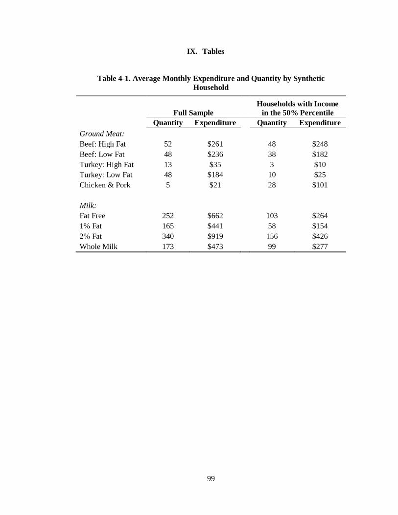
99

IX. Tables

Table 4-1. Average Monthly Expenditure and Quantity by Synthetic

Household

Full Sample

Households with Income

in the 50% Percentile

Quantity Expenditure

Quantity Expenditure

Ground Meat:

Beef: High Fat 52 $261

48 $248

Beef: Low Fat 48 $236

38 $182

Turkey: High Fat 13 $35

3 $10

Turkey: Low Fat 48 $184

10 $25

Chicken & Pork 5 $21

28 $101

Milk:

Fat Free 252 $662

103 $264

1% Fat 165 $441

58 $154

2% Fat 340 $919

156 $426

Whole Milk 173 $473 99 $277

100

Table 4-2(a). Summary Statistics of Sample: Ground Meat Category

Mean Std. Dev.

Budget Shares

Beef: High Fat 0.35 0.17

Beef: Low Fat 0.34 0.16

Turkey: High Fat 0.02 0.03

Turkey: Low Fat 0.29 0.20

Chicken & Pork 0.01 0.02

Monthly Expenditure on Category by

Synthetic HH $586 $501

Household size 2.57 0.16

Percentage of population that is black 9.8% 8.01

Annual Income per Synthetic HH $57,857 $8,193

Percentage of HH heads that are male 78% 4.32

101

Table 4-2(b). Summary Statistics of Sample: Milk Category

Mean Std. Dev.

Budget Shares

1% Fat Milk 0.16 0.13

2% Fat Milk 0.39 0.17

Whole Milk 0.22 0.16

Fat-free Milk 0.22 0.15

Monthly Expenditure on Category by

Synthetic HH $2,454 $2,316

Household size 2.48 0.24

Percentage of population that is black 8.7% 6.3

Annual Income per Synthetic HH $42,959 $22,978

Percentage of HH heads that are male 71% 10.21

102

Table 4-3. Habit Formation Parameter Estimates

φi Standard Errors

Ground Meat Beef: High Fat 0.496*** (0.0052)

Beef: Low Fat 0.484*** (0.0051)

Turkey: High Fat 0.553*** (0.0069)

Turkey: Low Fat 0.495*** (0.0051)

Chicken & Pork 0.375*** (0.0189)

Milk

1% Fat 0.060*** (0.0065)

2% Fat 0.067*** (0.0059)

Whole 0.073*** (0.0061)

Fat-free 0.069*** (0.0168)

*** p<0.01, **p<0.05, *p<0.1

103

Table 4-4. Long Run Unconditional Own and Cross-Price Elasticities

Ground Meat

Beef:

High Fat

Beef:

Low Fat

Turkey:

High Fat

Turkey:

Low Fat

Chicken

& Pork

Beef: High Fat -.899*** -.044*** -.005** -.064*** -.002**

Beef: Low Fat -.033*** -.727*** -.008*** -.222*** -0.005***

Turkey: High Fat -.010* .042*** -.968*** .038*** .023***

Turkey: Low Fat -.057*** -.209*** -.003 -.703*** .008***

Chicken & Pork .068 -.582*** -.056*** -.487*** -1.28***

Milk 1% Fat 2% Fat Whole Fat-free

1% Fat -0.732*** -.067*** -.1538*** -.065**

2% Fat -.056*** -.576*** -.219*** -.146***

Whole -.144*** -.203*** -.448*** .175***

Fat-free -.058*** -0.14*** .170*** -0.623***

*** p<0.01, **p<0.05, *p<0.1

104

REFERENCES

Adams, E. J., Grummer-Strawn, L., & Chavez, G. (2003). Food insecurity is associated

with increased risk of obesity in California women. The Journal of Nutrition, 133(4),

1070-1074.

Anderson, M. L., & Matsa, D. A. (2011). Are restaurants really supersizing

America? American Economic Journal: Applied Economics, 152-188.

Andreyeva, T., Luedicke, J., Henderson, K. E., & Tripp, A. S. (2012). Grocery store

beverage choices by participants in federal food assistance and nutrition

programs. American Journal of Preventive Medicine, 43(4), 411-418.

Astrup, A. (2005). The role of dietary fat in obesity. In Seminars in Vascular

Medicine (Vol. 5, No. 1, pp. 40-47).

Autor, D. H. (2003). Outsourcing at will: The contribution of unjust dismissal doctrine to

the growth of employment outsourcing. Journal of Labor Economics, 21(1), 1-42.

Basiotis, P. P., & Lino, M. (2003). Food insufficiency and prevalence of overweight

among adult women. Family Economics and Nutrition Review,15(2), 55.

Baum, C. L. (2011). The Effects of Food Stamps on Obesity. Southern Economic

Journal, 77(3), 623-651.

Beatty, T. K. M., and Tuttle, C. J. (2015). Expenditure response to in-kind transfers:

evidence from the Supplemental Nutrition Assistance Program. American Journal of

Agricultural Economics, 97(2), 390-404.

Becker, G. S., & Murphy, K. M. (1988). A theory of rational addiction. Journal of

Political Economy, 96(4), 675-700.

Binkley, J. K. (2008). Calorie and gram differences between meals at fast food and table

service restaurants. Applied Economic Perspectives and Policy,30(4), 750-763.

Biro, F. M., & Wien, M. (2010). Childhood obesity and adult morbidities. The American

Journal of Clinical Nutrition, 91(5), 1499S-1505S.

Bleich, S. N., Vine, S., & Wolfson, J. A. (2013). American adults eligible for the

Supplemental Nutritional Assistance Program consume more sugary beverages than

ineligible adults. Preventive Medicine, 57(6), 894-899.

Boonsaeng, T., Carpio, C. E., Zhen, C., & Okrent, A. M. (2012). The effect of

Supplemental Nutrition Assistance Program on food spending among low-income

households. In Selected Paper prepared for presentation at the Agricultural &

Applied Economics Association’s 2012 AAEA Annual Meeting, Seattle, Washington.

105

Bowman, Shanthy A., Steven L. Gortmaker, Cara B. Ebbeling, Mark A. Pereira, and

David S. Ludwig. (2004). Effects of fast-food consumption on energy intake and diet

quality among children in National Household Survey. Pediatrics 113(1): p. 112-18.

Bray, G. A., & Popkin, B. M. (1998). Dietary fat intake does affect obesity!. The

American Journal of Clinical Nutrition, 68(6), 1157-1173.

Bray, G. A., Paeratakul, S., & Popkin, B. M. (2004). Dietary fat and obesity: a review of

animal, clinical and epidemiological studies. Physiology & Behavior, 83(4), 549-555.

Bridging The Gap. State Sales Taxes on Soda, Bottled Water, and Snack Foods [Data

File]. Retrieved from

http://www.bridgingthegapresearch.org/research/sodasnack_taxes/

Briz, J., Ward, R., & De Felipe, I. (1998). Habit formation and demand system estimates

for fluid milk in Spain. The International Food and Agribusiness Management

Review, 1(4), 477-493.

Browning, M., & Collado, M. D. (2007). Habits and heterogeneity in demands: a panel

data analysis. Journal of Applied Econometrics, 22(3), 625-640.

Bruich, G. A. (2014). The effect of SNAP benefits on expenditures: New evidence from

scanner data and the November 2013 benefit cuts. Harvard University. Mimeograph,

September.

Bruijn, G. J., Kroeze, W., Oenema, A., & Brug, J. (2008). Saturated fat consumption and

the theory of planned behaviour: Exploring additive and interactive effects of habit

strength. Appetite, 51(2), 318-323.

Burgstahler, R., Gundersen, C., & Garasky, S. (2012). The Supplemental Nutrition

Assistance Program, financial stress, and childhood obesity. Agricultural and

Resource Economics Review, 41(1), 29.

Capps, O. (1989). Utilizing scanner data to estimate retail demand functions for meat

products. American Journal of Agricultural Economics, 71(3), 750-760.

Carrasco, R., Labeaga, J. M., & David López‐Salido, J. (2005). Consumption and habits:

Evidence from panel data. The Economic Journal, 115(500), 144-165.

Centers for Disease Control and Prevention. (2003). Self-reported concern about food

security associated with obesity--Washington, 1995-1999. MMWR. Morbidity and

Mortality Weekly Report, 52(35), 840.

Chen, X., H. M. Kaiser, and B. J. Rickard. (2015). "The Impacts of inclusive and

exclusive taxes on healthy eating: An experimental study." Food Policy 56:13-24.

Chen, Z., Yen, S. T., & Eastwood, D. B. (2005). Effects of food stamp participation on

body weight and obesity. American Journal of Agricultural Economics, 87(5), 1167-

1173.

http://www.bridgingthegapresearch.org/research/sodasnack_taxes/

106

Chetty, R., A. Looney, and K. Kroft. (2009). "Salience and taxation: Theory and

evidence." American Economic Review 99(4):1145-1177.

Chouinard, H. H., Davis, D. E., LaFrance, J. T., & Perloff, J. M. (2007). Fat taxes: big

money for small change. In Forum for Health Economics & Policy, 10(2), p. 2. De

Gruyter.

Currie, J., DellaVigna, S., Moretti, E., & Pathania, V. (2010). The effect of fast food

restaurants on obesity and weight gain. American Economic Journal: Economic

Policy, 32-63.

Dietz, W. H. (1995). Does hunger cause obesity?. Pediatrics, 95(5), 766-767.

Dinour, L. M., Bergen, D., & Yeh, M. C. (2007). The food insecurity–obesity paradox: a

review of the literature and the role food stamps may play. Journal of the American

Dietetic Association, 107(11), 1952-1961.

Dynan, K. E. (2000). Habit formation in consumer preferences: Evidence from panel

data. American Economic Review, 391-406.

Economic Research Service. (2013). Supplemental Nutrition Assistance Program (SNAP)

Data System [Data file]. Retrieved on April 19, 2016 from

http://www.ers.usda.gov/data-products/supplemental-nutrition-assistance-program-

(snap)-data-system/time-series-data.aspx

Fernandes, M. M. (2012). Effect of the Supplemental Nutrition Assistance Program

(SNAP) on frequency of beverage consumption among youth in the United

States. Journal of the Academy of Nutrition and Dietetics, 112(8), 1241-1246.

Fox, M. K., Hamilton, W., Lin, B. H. (2004). Effects of food assistance and nutrition

programs on nutrition and health. Food Assistance and Nutrition Research Report

(No. 19-3). United States Department of Agriculture, Economic Research Service.

Frongillo, E. A., Jr., Olson, C. M., Rauschenbach, B. S. & Kendall, A. (1997). Nutritional

consequences of food insecurity in a rural new york state county. Discussion Paper

no. 1120–97. Institute for Research on Poverty, University of Wisconsin, Madison,

WI.

Garasky, S., Mbwana, K., Romualdo, A., Tenaglio, A., and Roy M. (2016). Foods

Typically Purchased by SNAP Households. Prepared by IMPAQ International, LLC

for USDA, Food and Nutrition Service, November 2016.

Gibson, D. (2003). Food stamp program participation is positively related to obesity in

low income women. The Journal of Nutrition, 133(7), 2225-2231.

Golay, A., & Bobbioni, E. (1997). The role of dietary fat in obesity. International

Journal of Obesity and Related Metabolic Disorders: Journal of the International

Association for the Study of Obesity, 21, S2-11.

http://www.ers.usda.gov/data-products/supplemental-nutrition-assistance-program-(snap)-data-system/time-series-data.aspx

http://www.ers.usda.gov/data-products/supplemental-nutrition-assistance-program-(snap)-data-system/time-series-data.aspx

107

Gregory, C. A., & Coleman-Jensen, A. (2013). Do high food prices increase food

insecurity in the United States? Applied Economic Perspectives and Policy, 35(4),

679-707.

Heien, D., & Durham, C. (1991). A test of the habit formation hypothesis using

household data. The Review of Economics and Statistics, 189-199.

Hoynes, H. W., and Schanzenbach, D. W. (2009). Consumption responses to in-kind

transfer: Evidence from the introduction of the Food Stamp Program. American

Economic Journal: Applied Economics, 1(4), 109-139.

Khare, A., & Inman, J. J. (2006). Habitual behavior in American eating patterns: The role

of meal occasions. Journal of Consumer Research, 32(4), 567-575.

Laird, E., & Trippe, C. (2014). Programs conferring categorical eligibility for SNAP:

state policies and the number and characteristics of households affected. Submitted

to the US Department of Agriculture, Food and Nutrition Service. Washington, DC:

Mathematica Policy Research.

Leung, C. W., Ding, E. L., Catalano, P. J., Villamor, E., Rimm, E. B., & Willett, W. C.

(2012). Dietary intake and dietary quality of low-income adults in the Supplemental

Nutrition Assistance Program. The American Journal of Clinical Nutrition, ajcn-

040014.

Levi, J., Segal, L. M., St Laurent, R., Kohn, D., (2011). F as in fat: how obesity threatens

America’s future 2012. Retrieved March 16, 2017 from

http://www.tfah.org/assets/files/TFAH2011FasInFat10.pdf

Mancino, L., Todd, J., & Lin, B. H. (2009). Separating what we eat from where:

measuring the effect of food away from home on diet quality. Food Policy, 34(6),

557-562.

Meyerhoefer, C. D., & Pylypchuk, Y. (2008). Does participation in the Food Stamp

Program increase the prevalence of obesity and health care spending? American

Journal of Agricultural Economics, 90(2), 287-305.

Muellbauer, J., & Pashardes, P. (1992). Tests of dynamic specification and homogeneity

in a demand system. In Aggregation, Consumption and Trade (pp. 55-98). Springer

Netherlands.

Naik, N. Y., & Moore, M. J. (1996). Habit formation and intertemporal substitution in

individual food consumption. The Review of Economics and Statistics, 321-328.

National Institute of Health. (2012). Overweight and Obesity Statistics. National Institute

of Diabetes and Digestive and Kidney Diseases report. Retrieved from

http://www.niddk.nih.gov/health-information/health-statistics/Pages/overweight-

obesity-statistics.aspx

http://www.tfah.org/assets/files/TFAH2011FasInFat10.pdf

http://www.niddk.nih.gov/health-information/health-statistics/Pages/overweight-obesity-statistics.aspx

http://www.niddk.nih.gov/health-information/health-statistics/Pages/overweight-obesity-statistics.aspx

108

Nguyen, B. T., Shuval, K., Njike, V. Y., & Katz, D. L. (2014). The Supplemental

Nutrition Assistance Program and dietary quality among US adults: findings from a

nationally representative survey. In Mayo Clinic Proceedings, 89(9), pp. 1211-1219.

Ogden C. L., Lamb, M. M., Carroll M. D., Flegal K. M. (2010) Obesity and

socioeconomic status in adults: United States 1988–1994 and 2005–2008. NCHS data

brief no 50. Hyattsville, MD: National Center for Health Statistics. Retrieved March

16, 2017 from https://www.cdc.gov/nchs/products/databriefs/db50.htm

Olson, C. M. (1999). Nutrition and health outcomes associated with food insecurity and

hunger. The Journal of Nutrition, 129(2), 521S-524S.

Paeratakul, S., D. Ferdinand, C. Champagne, D. Ryan, and G. Bray. (2003). Fast food

consumption among U.S. adults and children: Dietary and nutrient intake profile.

Journal of the American Dietetic Association, 103(10): p. 1332-38, 2003

Ratcliffe, C., McKernan, S. M., & Zhang, S. (2011). How much does the Supplemental

Nutrition Assistance Program reduce food insecurity? American Journal of

Agricultural Economics, 93(4): 1082–1098.

Richards, T. J., Patterson, P. M., & Tegene, A. (2007). Obesity and nutrient consumption:

a rational addiction?. Contemporary Economic Policy, 25(3), 309-324.

Robinson, C. A., & Zheng, X. (2011). Household Food Stamp Program Participation and

Childhood Obesity. Journal of Agricultural and Resource Economics, 36(1), 1.

Rosinger, A., Herrick, K., Gahche, J., Park, S., Frank, S. (2017). QuickStats: Percentage

of total daily kilocalories consumed from sugar-sweetened beverages among children

and adults, by sex and income level — National Health and Nutrition Examination

Survey, United States. MMWR Morb Mortal Wkly Rep 2017; 66:181.

Serdula, M. K., Ivery, D., Coates, R. J., Freedman, D. S., Williamson, D. F., & Byers, T.

(1993). Do obese children become obese adults? A review of the

literature. Preventive medicine, 22(2), 167-177.

Smed, S., Jensen, J. D., & Denver, S. (2007). Socio-economic characteristics and the

effect of taxation as a health policy instrument. Food Policy, 32(5), 624-639.

Todd, J. E., Mancino, L., & Lin, B. H. (2010). The impact of food away from home on

adult diet quality. USDA-ERS Economic Research Report Paper, (90).

Todd, J. E., & Morrison, R. M. (2014). Less eating out, improved diets, and more family

meals in the wake of the great recession. Amber Waves, 1E.

Todd, J. E., & Ver Ploeg, M. (2014). Caloric beverage intake among adult Supplemental

Nutrition Assistance Program participants. American Journal of Public Health,

104(9), e80-e85.

https://www.cdc.gov/nchs/products/databriefs/db50.htm

109

Townsend, M. S., Peerson, J., Love, B., Achterberg, C., & Murphy, S. P. (2001). Food

insecurity is positively related to overweight in women. The Journal of Nutrition,

131(6), 1738-1745.

US Census Bureau. (2015). Current Population Survey, 2015 Annual Social and

Economic Supplement [Data file]. Retrieved from ftp://ftp2.census.gov/programs-

surveys/cps/techdocs/cpsmar15.pdf.

Watt, T. T., Appel, L., Roberts, K., Flores, B., & Morris, S. (2013). Sugar, stress, and the

supplemental nutrition assistance program: Early childhood obesity risks among a

clinic-based sample of low-income hispanics. Journal of Community Health, 38(3),

513-520.

Wilde, P. E., & Ranney, C. K. (2000). The monthly food stamp cycle: Shopping

frequency and food intake decisions in an endogenous switching regression

framework. American Journal of Agricultural Economics, 82(1), 200-213.

Yen, S. T., Andrews, M., Chen, Z., & Eastwood, D. B. (2008). Food Stamp Program

participation and food insecurity: An instrumental variables approach. American

Journal of Agricultural Economics, 90(1), 117-132.

Zhen, C., Wohlgenant, M. K., Karns, S., & Kaufman, P. (2011). Habit formation and

demand for sugar-sweetened beverages. American Journal of Agricultural

Economics, 93(1), 175-193.

Zheng, Y., E.W. McLaughlin, and H.M. Kaiser. (2013). Taxing food and beverages:

Theory, evidence, and policy. American Journal of Agricultural Economics

95(3):705-723.

ftp://ftp2.census.gov/programs-surveys/cps/techdocs/cpsmar15.pdf

ftp://ftp2.census.gov/programs-surveys/cps/techdocs/cpsmar15.pdf

110

VITA

SHAHEER BURNEY

EDUCATION

M.S., Economics, University of Kentucky, Lexington, KY Dec. 2014

M.B.A., University of Louisville, Louisville, KY Sept. 2011

B.A., Economics & Mathematics, Hanover College, Hanover, IN May 2010

PROFESSIONAL POSITIONS

Postdoctoral Fellow, Zwick Center for Food and Resource Policy, Department of

Agricultural and Resource Economics, University of Connecticut, Storrs, CT. May 2017

– Present

Graduate Research Assistant, Department of Agricultural Economics, University of

Kentucky, Lexington, KY. Aug. 2012 – Apr. 2017

Visiting Researcher, Department of Agricultural and Resource Economics, University of

California – Berkeley. Aug. 2015 to Dec. 2015

Research Assistant, University of Louisville, Department of Economics, Louisville, KY

Nov. 2011 – July 2012

THE ROLE OF SNAP AND HABIT FORMATION ON HOUSEHOLD ...

Documents

Transcript of THE ROLE OF SNAP AND HABIT FORMATION ON HOUSEHOLD ...