1  

The Role of the Atmosphere in the Provision of Ecosystem Services 1 

 2 

*Ellen J. Cooter1, Anne Rea1, Randy Bruins2, Donna Schwede1, Robin Dennis1 3 

 4 

1\ U.S. Environmental Protection Agency, National Exposure Research Laboratory, 5 

Research Triangle Park, North Carolina 6 

2\ U.S. Environmental Protection Agency, National Exposure Research Laboratory, 7 

Cincinnati, Ohio 8 

 9 

 10 

 11 

 12 

For Submission to 13 

Science of the Total Environment 14 

Special Issue Honoring Jerry Keeler 15 

 16 

 17 

 18 

*Corresponding author 19 

U.S. EPA National Exposure Research Lab 20 

Mail Drop E‐243‐02 21 

Research Triangle Park, North Carolina 22 

USA 23 

Cooter.ellen@epa.gov 24 

Phone:  919‐541‐1334; FAX: 919‐541‐1379   25 

2  

Abstract 26 

Solving the environmental problems that we are facing today requires holistic approaches 27 

to analysis and decision making that include social and economic aspects. The concept of 28 

ecosystem services, defined as the benefits people obtain from ecosystems, is one potential tool 29 

to perform such assessments. The objective of this paper is to demonstrate the need for an 30 

integrated approach that explicitly includes the contribution of atmospheric processes and 31 

functions to the quantification of air-ecosystem services. First, final and intermediate air-32 

ecosystem services are defined. Next, an ecological production function for clean and clear air is 33 

described, and its numerical counterpart (the Community Multiscale Air Quality Model) is 34 

introduced. An illustrative numerical example is developed that simulates potential changes in 35 

air-ecosystem services associated with the conversion of evergreen forest land in Mississippi, 36 

Alabama and Georgia to commercial crop land. This one-atmosphere approach captures a broad 37 

range of service increases and decreases. Results for the forest to cropland conversion scenario 38 

suggest that although such change could lead to increased biomass (food) production services, 39 

there could also be coincident, seasonally variable decreases in clean and clear air-ecosystem 40 

services (i.e., increased levels of ozone and particulate matter) associated with increased 41 

fertilizer application. Metrics that support the quantification of these regional air-ecosystem 42 

changes require regional ecosystem production functions that fully integrate biotic as well as 43 

abiotic components of terrestrial ecosystems, and do so on finer temporal scales than are used for 44 

the assessment of most ecosystem services. 45 

46 

47 

Keywords: ecosystem services; CMAQ; quantification of air-ecosystem services; air quality 48 

modeling; clean air services 49 

50 

3  

1.0 Introduction 51 

Solving the environmental problems that we are facing today requires holistic approaches 52 

to analysis and decision-making. Issues such as global climate change, land use change resulting 53 

from increasing human population, and long-term anthropogenic impacts on global 54 

biogeochemical cycles cannot be considered as isolated problems or individual research topics. 55 

To address the full implications of our decisions across local, national, and global scales and 56 

multiple human generations we must adopt a broad, systems perspective that incorporates social, 57 

environmental, and economic aspects. The U.S. National Research Council has referred to these 58 

as “the three pillars of sustainability” (National Research Council, 2011). 59 

Recently the concept of ecosystem services, defined as the benefits people obtain from 60 

ecosystems, has been used to show how humans benefit from the natural capital provided by the 61 

earth (MEA, 2005). Valuing the benefits we receive from nature, and identifying the 62 

beneficiaries, allows for a more complete assessment of the social, environmental, and economic 63 

impacts of a given management action or policy decision leading to maximum benefits 64 

(including benefits to human health) and fewer unintended consequences. For example, 65 

quantification of wetland value based on the ecosystem services it provides to the local 66 

community may inform decision makers when evaluating the utility of that wetland relative to 67 

the benefits of urban development. The value of services provided by the atmosphere has rarely 68 

been considered in detail (Thornes et al., 2010). In response, Thornes et al. (2010) provide 69 

initial estimates for 12 atmospheric services; a total value that ranges from 100 to 1000 times the 70 

2008 Gross World Product. These estimates are based on a value relative to Carbon Dioxide 71 

under the EUETS (European Union Emissions Trading Scheme), and value relative to 72 

compressed air. The authors note that additional research is needed to develop a more systematic 73 

4  

approach to the valuation of specific atmospheric services. Challenges to the development of 74 

such an approach include those encountered when valuing any natural resource (see, e.g., 75 

Randall, 1987), but also include the tendency to treat the atmosphere as a source of hazard as 76 

opposed to benefit, and an artificial distinction between atmospheric and ecosystem services. In 77 

reality, ecosystems comprise biotic and abiotic components that cannot exist independent of one 78 

another, and together provide beneficial services to humans. The term air-ecosystem service is 79 

used throughout this discussion to emphasize that the integrated, co-dependent nature of this 80 

relationship must be considered. We begin by defining what is meant by the term “air-ecosystem 81 

service.” This is followed by the exploration of a conceptual model detailing the tightly coupled 82 

nature of one specific air-ecosystem service; clean air. A crucial step towards the economic 83 

valuation of ecosystem services is the quantification of services using metrics that can be linked 84 

to economically valued benefits. A regional air quality model that quantitatively defines many 85 

aspects of the response of a tightly coupled atmosphere-biosphere system is used to illustrate 86 

connections between human behavior and preferences and the underlying ecological processes 87 

and functions leading to the production of clean air ecosystem services. This example is 88 

followed by a discussion of clean air-ecosystem services in the context of environmental 89 

economics and management. 90 

91 

2.0 Methodology 92 

93 

2.1 Defining and Classifying Air-Ecosystem Services 94 

Two recent views regarding air-ecosystem interactions are presented in Berkowicz (2010) 95 

and Thornes et al. (2010). Both discussions treat the atmosphere and its processes as linked 96 

5  

with, but external to, biological systems. However, these systems are, in fact tightly coupled, 97 

and failure to treat them as such in decision making can lead to unanticipated consequences. 98 

Pielke et al. (2007) provide examples of such consequences resulting from regional land-use and 99 

land-cover changes. Decreases in local temperature, increased cloud cover and, under some 100 

conditions, increased precipitation have been reported in response to the conversion of grassland 101 

to irrigated crop agriculture in the Great Plains of the U.S.; such changes can lead to greater 102 

biologic production in rainfed and irrigated systems. By contrast, observational studies of 103 

widespread tropical deforestation report rainfall decreases of 1 to 20% as the result of changes in 104 

evaporation, transpiration, surface albedo and aerodynamic roughness. These atmospheric 105 

interactions can exacerbate water quantity and quality problems resulting from altered surface 106 

runoff characteristics. Urbanization of natural landscapes restructures the local energy budget, 107 

leading to increased temperatures and modified diurnal temperature patterns, wind and humidity 108 

fields (Landsberg, 1981). These factors impact human health (e.g., heat- and air-quality related 109 

morbidity and mortality), local economies (e.g., energy, storage and transportation costs), and 110 

may further combine with anthropogenic changes in the aerosol environment to alter patterns of 111 

urban precipitation frequency and intensity (Shepherd and Burian, 2003). Studies such as these 112 

have led to a more holistic understanding of the tightly coupled interactions among the 113 

atmosphere, the biosphere and human society. We propose that same approach be applied to the 114 

quantification, valuation and sustainability of air-ecosystem services following the proposals of 115 

Constanza (2008) and Fisher et al. (2009), that any definition or classification of services should 116 

be context-dependent and should address issues of sustainability. 117 

A holistic, systems-based approach begins by recognizing that an ecosystem comprises 118 

both biotic and abiotic (e.g., air, water, land) components. Ecosystem services are, therefore, 119 

6  

outputs of ecological functions or processes of these interacting biotic and abiotic components 120 

that directly or indirectly contribute to social welfare or have the potential to do so in the future 121 

(USEPA, 2006c). Ecosystem services can be classified in many ways. The Millennium 122 

Ecosystem Assessment (MEA) defines and classifies ecosystem services into several categories: 123 

Ecosystem services are the benefits people obtain from ecosystems. 124 

These include provisioning services such as food, water, timber, and 125 

fiber; regulating services that affect climate, floods, disease, wastes, and 126 

water quality; cultural services that provide recreational, aesthetic, and 127 

spiritual benefits; and supporting services such as soil formation, 128 

photosynthesis, and nutrient cycling (MEA, 2005). 129 

While useful, this definition is somewhat ambiguous and does not facilitate explicit linkage 130 

between ecological assessment and the economic valuation of changes in these services. Most 131 

importantly, it lends itself to double counting of benefits (Fisher et al., 2009). To avoid these 132 

pitfalls, Boyd and Banzhaf (2007) propose that an effective classification scheme should 133 

distinguish between final ecosystem services, intermediate ecosystem services and benefits. 134 

Since this paper focuses on exploring the biophysical quantification of air-ecosystem services in 135 

preparation for benefits assessment and valuation, this expanded classification is more 136 

appropriate. A final ecosystem service is a component of nature, directly enjoyed, consumed, or 137 

used to yield human well-being. That is, final ecosystem services are outputs or end products of 138 

ecological processes that either directly result in human benefits or, when combined with human, 139 

social or built capital, produce human benefits. Fisher et al. (2009) expand this definition to 140 

include ecosystem organization or structure if they are consumed or utilized by humanity. An 141 

intermediate ecosystem service is a service that is necessary for the production of final ecosystem 142 

7  

services. For example, intermediate ecosystem services (endpoints) including habitat, 143 

biodiversity and clean water are necessary for the production of healthy recreational fish 144 

populations (final service). Benefits, however, do not accrue without the addition of roads, boat 145 

ramps, etc. to provide access to the service. 146 

A hierarchy of air-ecosystem services utilizing these definitions is presented in Figure 1. 147 

In this hierarchy, clean air and climate and weather are final air-ecosystem services. Information 148 

regarding beneficiaries, atmospheric metrics, linkages to biologic components as well as 149 

example benefits and valuation metrics are provided in Tables 1 and 2. Clear air (Table 1) 150 

focuses on issues of visibility with principal beneficiaries being the transportation and 151 

recreational sectors. Some metrics for these services include visual quality and range. Example 152 

benefits include reduced death/injury from accidents, improved delivery efficiency (e.g., can 153 

travel faster, fewer delays) and visitor viewing enjoyment (day and night). Clean air is closely 154 

related to clear air services, but in this case, beneficiaries include sensitive human and natural 155 

(e.g., vegetation, fish, wildlife, etc) subpopulations. Some metrics describing the quantity of 156 

clean air include hourly pollutant concentrations, air quality indices, the assimilative capacity of 157 

the atmosphere before unhealthy concentrations are experienced, and cumulative exposure 158 

metrics for humans, e.g. daily maximum 8 hr average ozone (MDA8), and for vegetation, e.g. 159 

W126 (USEPA, 2006a; USEPA, 2006c). Some metrics that quantify benefits derived from clean 160 

air for vegetation include appearance and biodiversity. Some metrics that quantify human 161 

benefits include reduced morbidity/mortality and hospital admissions in response to changes in 162 

pollutant concentration levels. 163 

Climate and weather is the third major class of final air-ecosystem service (Table 2). 164 

Some components of climate and weather that are directly enjoyed and, therefore, are final 165 

8  

services include a pleasant or livable environment and water quantity. The beneficiaries of a 166 

livable environment are the recreation sector, the general public and sensitive life-stages such as 167 

the very young or elderly. The quantity of pleasant environment directly experienced or enjoyed 168 

can be expressed through a number of human comfort indices that are a function of heat/cold, 169 

wind and humidity (see examples at. http://www.nws.noaa.gov/os/heat/index.shtml#heatindex 170 

and http://www.nws.noaa.gov/os/windchill/index.shtml ). Some metrics that quantify the benefits of 171 

a livable climate are measured in terms of reduced heat/cold related morbidity, mortality and 172 

hospital admissions. 173 

The final climate and weather service, water quantity, specifically applies to aspects of 174 

precipitation that are directly consumed or enjoyed such as maintenance of drinking water 175 

supplies and recreational activities requiring a specific volume or depth of water such as 176 

swimming, boating, snow skiing or snowmobiling. The beneficiaries are the general and 177 

recreating public. The service is measured in terms of precipitation depth or runoff volume. 178 

Such benefits are quantified by lake levels or the size of the recreational pool of a reservoir. 179 

In addition to final services, Figure 1 indicates that there also can be climate and weather 180 

services such as the provision of temperature, precipitation and radiation conditions that are 181 

conducive (intermediate) to the production of clean water and biomass production final services. 182 

For example, returning to the earlier example of the conversion of grassland to irrigated 183 

cropland, the atmosphere provides intermediate services in the form of surface temperature and 184 

precipitation towards the provision of the final service “crop biomass” which is consumed in the 185 

form of food. The coupled interaction of the biologic community response to irrigation (i.e., 186 

seasonal changes, albedo, leaf area, surface roughness and moisture flux, in addition to 187 

additional moisture flux from the irrigation itself) are credited with the temperature and 188 

9  

precipitation changes noted previously. Corn, an important food crop grown in the Great Plains, 189 

is particularly sensitive to high temperatures during flowering (anthesis). Any reduction from 190 

normal maximum daily temperatures at this critical crop stage can affect corn yield. Periodic 191 

increases in precipitation can result in reduced irrigation demand to stave-off yield losses 192 

associated with water stress. Table 3 contains selected examples in which climate and weather 193 

services are intermediate to the production of biomass and clean water final ecosystem services. 194 

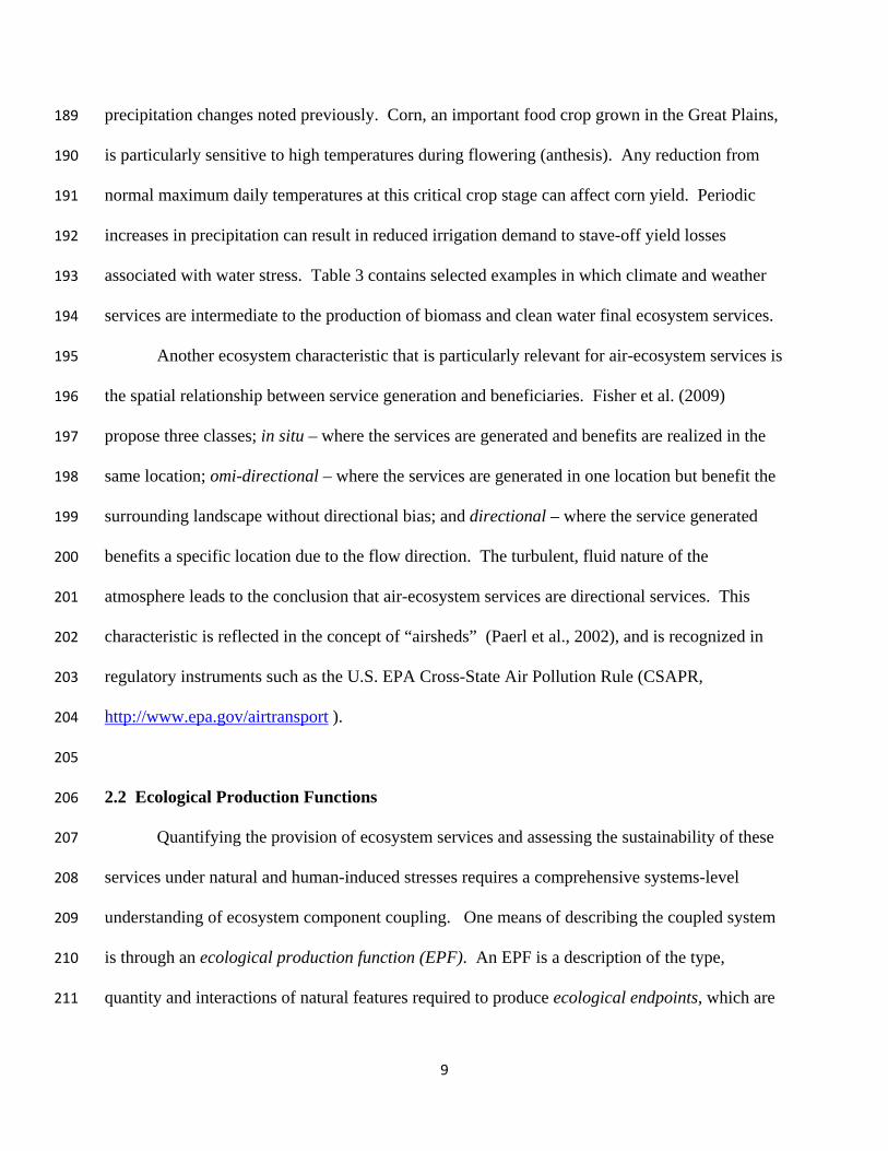
Another ecosystem characteristic that is particularly relevant for air-ecosystem services is 195 

the spatial relationship between service generation and beneficiaries. Fisher et al. (2009) 196 

propose three classes; in situ – where the services are generated and benefits are realized in the 197 

same location; omi-directional – where the services are generated in one location but benefit the 198 

surrounding landscape without directional bias; and directional – where the service generated 199 

benefits a specific location due to the flow direction. The turbulent, fluid nature of the 200 

atmosphere leads to the conclusion that air-ecosystem services are directional services. This 201 

characteristic is reflected in the concept of “airsheds” (Paerl et al., 2002), and is recognized in 202 

regulatory instruments such as the U.S. EPA Cross-State Air Pollution Rule (CSAPR, 203 

http://www.epa.gov/airtransport ). 204 

205 

2.2 Ecological Production Functions 206 

Quantifying the provision of ecosystem services and assessing the sustainability of these 207 

services under natural and human-induced stresses requires a comprehensive systems-level 208 

understanding of ecosystem component coupling. One means of describing the coupled system 209 

is through an ecological production function (EPF). An EPF is a description of the type, 210 

quantity and interactions of natural features required to produce ecological endpoints, which are 211 

10  

defined as any biophysical feature, quantity, or quality that requires little further translation to 212 

make clear its relevance to human well-being. Additionally, an EPF can be thought of as 213 

describing the relationship between intermediate services, final services and benefits (Ringold et 214 

al., 2009). Therefore, the outputs of EPFs, when combined with inputs that allow ecological 215 

goods or services to be used (e.g., roads or site accessibility) produce benefits (Wainger and 216 

Mazzotta, 2009; Wainger and Boyd, 2009). 217 

As an example, the biophysical characteristics of a coastal wetland (flooding regimes, 218 

salinity, nutrient concentrations, plant species abundance, predator and prey abundances, climate, 219 

etc.) can influence the abundance of a population of watchable wading shorebirds (the ecological 220 

endpoint). An EPF describing these complex relationships would be useful for estimating the 221 

potential of different coastal wetlands to provide bird-watching recreational services, if other 222 

inputs (e.g., boardwalks or kayak launch points) were also present. Moreover, the relevance to 223 

sustainability of such an EPF would be increased if, (a) its dependent variables or outputs (i.e., 224 

the species predicted) aligned well to birdwatchers’ preferences, (b) its independent variables or 225 

inputs (i.e., wetland characteristics) were feasibly measured, and (c) critical design factors for 226 

enhancing or restoring those characteristics, in cases where wetlands had been degraded or 227 

destroyed, were also incorporated into the EPF. There are several benefits and ecosystem 228 

services related to this example that are unidentified, unquantified, and unmonetized, ranging 229 

from clean water services and biodiversity to aesthetics and nonuse values (USEPA, 2006c). 230 

With these characteristics in mind, we describe an EPF for clean air-ecosystem services 231 

associated with clear and healthful air below. 232 

233 

2.3 A Conceptual Air-Ecosystem Service EPF 234 

11  

The tight coupling of biotic and abiotic ecosystem components required to produce the 235 

final air-ecosystem services of clean air and clear air that includes two-way feedbacks among the 236 

biosphere, atmosphere, weather and pollution is described conceptually in Figure 2. The primary 237 

processes involved in the provision of clean air services are the production (emission), 238 

transformation, dilution, and removal of harmful or potentially harmful (precursor) chemicals 239 

from the atmosphere. An EPF can be used to explore how differences in factors that affect these 240 

processes, such as land use, meteorology and emissions and interactions among these processes 241 

and factors can result in changes in the quantity of clean air, i.e., air quality experienced by 242 

humans. As in the previous example for wetlands, an EPF that is suited to addressing the 243 

sustainability of clean air services must be able to account for aspects of human and societal need 244 

or preference, as well as behaviors that can exacerbate or ameliorate threats to those services by 245 

affecting the magnitude of the underlying processes. An overview of processes that should be 246 

included in a clean air EPF follows. 247 

Our EPF (Figure 2) begins with the introduction into our system of upstream or boundary 248 

air containing some level of natural and anthropogenic chemical constituents (upper left). Most 249 

unhealthful atmospheric constituents are either emitted directly into the atmosphere as the result 250 

of economic and social activity, e.g., power production, vehicular traffic, or are produced as the 251 

result of complex reactions within the atmosphere itself. Some of these emissions are deposited 252 

or transformed into other species near their sources, while the remainder may be transported out 253 

of the immediate area to later combine with additional downstream sources. Air pollutant 254 

emissions come from anthropogenic sources as well as managed and natural ecosystems. In 255 

Figure 2, sulfur dioxide (SO2), carbon monoxide (CO), nitrogen oxide (NO) and many volatile 256 

organic chemicals (VOC’s) come primarily from anthropogenic sources, e.g., stationary sources 257 

12  

(power plants) and mobile sources (gasoline and diesel fueled vehicles). The majority of 258 

ammonia (NH3) emissions are due to livestock agriculture, but emission of NH3, NO and nitrous 259 

oxide (N2O), a powerful greenhouse gas, from agricultural soils represents a nexus of human 260 

activity (fertilizer application) and ecosystem function (nitrification and denitrification). 261 

Biogenic emissions from managed as well as natural sources are an important source of VOCs 262 

that can lead to the formation of secondary aerosols (haze) that can enhance (e.g., Blue 263 

Mountains of Australia and Smokey Mountains of the U.S.) or degrade (e.g., U.S. Grand 264 

Canyon) recreational viewing opportunities in natural areas(Geron et al., 1994; Lamb et al., 265 

1993). 266 

Interactions between the biosphere and atmospheric processes contribute to the 267 

production of atmospheric pollutants by natural and managed ecosystems. For instance, natural 268 

or man-altered land surfaces such as waterbodies, inundated wetlands and irrigated agricultural 269 

fields add large supplies of moisture (humidity) to the atmosphere through evapotranspiration. 270 

Moisture fluxes, combined with boundary layer mixing, can fuel the formation of clouds. 271 

Primary and secondary aerosols also play a key role in the formation of clouds, e.g., act as cloud 272 

nuclei, and can participate in cloud aqueous chemistry to form atmospheric acids. In addition, 273 

there are feedback effects of aerosols on radiative forcing. While these feedback effects are 274 

mainly important for climate applications, it is becoming evident that they have substantial 275 

effects on local meteorology and air quality in polluted regions (Jacobson et al., 1996; Wong et 276 

al., 2012). Production of oxides of nitrogen by lightning activity associated with convective 277 

clouds is recognized as an important pollutant source (DeCaria et al., 2005; Ott et al., 2007). 278 

While the presence of clouds may enhance some chemical transformation, many other important 279 

atmospheric chemical reactions such as those that produce ozone (O3) are photolytic, i.e. driven 280 

13  

by light energy and are inhibited by the presence of clouds. Isoprene, a VOC emitted by some 281 

vegetation species, is a precursor chemical for O3, particulate matter (PM) and formaldehyde 282 

formation. Monoterpenes, another class of biogenic VOC produced by vegetation, can be 283 

oxidized by O3, hydroxyl radical and nitrate radical to form products that readily partition into 284 

aerosols that can lead to haze and compromise visibility. Ammonia contributes to the formation 285 

of ammonium aerosol, which is a major constituent of fine particulate matter (PM2.5) and VOCs, 286 

and NO can react with nitrogen dioxide (NO2) to produce ozone and additional particulate 287 

matter. At sufficiently high levels, oxidized and reduced N species, O3 and PM2.5 are all 288 

detrimental to human health and well-being (McConnell et al., 2002; von Mutius, 2000; Wolfe 289 

and Patz, 2002). 290 

Chemicals in the atmosphere are vertically or horizontally mixed into more or less 291 

reactive environments to either increase or dilute ambient concentrations. Two drivers of 292 

boundary layer mixing that link directly with ecosystem structure and function are convective 293 

and roughness-driven mixing. Convective mixing is driven by the flux of heat from underlying 294 

surfaces. Ecosystem features that directly impact surface temperature (as illustrated by the 295 

temperature values along the bottom of Figure 2) include overall surface reflectivity ( e.g., snow 296 

cover vs. dark organic soils), and the heat capacity of the surface ( e.g., leaves vs. water vs. soil). 297 

Roughness-driven mixing results when the free movement of air across a landscape is impeded 298 

by obstacles extending above an underlying surface. Some ecosystem features that can 299 

contribute to roughness-driven mixing include landscapes with varying patterns of vegetation 300 

heights and densities, and the extent and orientation of vegetated or non-vegetated corridors. 301 

Thus, both horizontal and vertical ecosystem structure contributes to the provision of clean air 302 

service through mixing-driven transport, dilution and deposition. 303 

14  

The underlying ecological structure and function also influence the removal of potentially 304 

harmful pollutants from the air. Precipitation can act to cleanse the atmosphere of harmful 305 

pollutants through wet deposition, but pollutants also are removed from the atmosphere through 306 

particle deposition to underlying surfaces and plant uptake of gases. The rate at which gases are 307 

removed is a function of surface wetness, strength of downward mixing, stomatal and cuticular 308 

vegetation conductance and leaf area. Stomatal and cuticular conductance can vary widely 309 

across vegetation species. For example, maximum stomatal conductance is much higher in 310 

grasses (0.01 m/s) than a broadleaf deciduous forest (0.005 m/s) (Xiu and Pleim, 2001). Forests, 311 

however, can have up to twice the intercepting leaf area per unit area leading to greater pollutant 312 

removal, and so the specific type of vegetation and vegetation density both contribute to the air 313 

pollutant removal efficiency. The rate of atmospheric particle deposition depends primarily on 314 

the particle size distribution and turbulence. (Grantz et al., 2003) 315 

316 

3.0 Analytical Framework 317 

318 

3.1 CMAQ as an Ecological Production Function 319 

Since the coupled atmospheric and biosphere system is complex with competing and 320 

compensating sources and sinks of pollutants and processes, a numerical model is a useful tool to 321 

quantify and characterize clean air endpoints, thereby serving as an EPF. For this analysis, we 322 

applied the Community Multiscale Air Quality (CMAQ) model (Byun and Schere, 2006) version 323 

4.7.1 as a clean and clear air EPF. CMAQ employs a 3-dimensional Eulerian modeling approach 324 

to address air quality issues such as tropospheric O3, PM2.5, air toxics, visibility and acid and 325 

nutrient deposition. The system comprises a meteorological modeling system for the description 326 

15  

of atmospheric conditions, emission models for anthropogenic and natural emissions that are 327 

injected into the atmosphere, and a chemical-transport modeling system (CTM) to simulate 328 

chemical transformations and atmospheric fate and transport. CMAQ can be used for both 329 

retrospective studies as well as analysis of future scenarios, allowing the investigation of 330 

potential environmental outcomes regarding air quality management. 331 

The meteorological model used in this example, the Weather Research Forecast model 332 

(WRF) (Skamarock et al., 2008), contains Land Surface Models (LSMs) that provide an 333 

interface between atmospheric processes and processes at the terrestrial surface. Land surface 334 

models simulate biophysical processes, soil hydrology, and surface heat and moisture fluxes to 335 

provide feedback to the atmosphere that, as described previously, may alter cloud, precipitation, 336 

and local and regional circulation. While current LSMs focus on surface fluxes affecting 337 

atmospheric processes with little regard for hydrology, they are becoming more sophisticated 338 

and are moving towards including dynamic vegetation modules, multi-layer vegetation canopy 339 

modules, terrestrial carbon and nitrogen cycling, irrigation treatment, surface and groundwater 340 

hydrology, transient land cover change and land-use change. The P-X land surface model is 341 

used in the present example (Pleim and Xiu, 2003). 342 

Biogenic emissions are estimated within CMAQ using the Biogenic Emissions Inventory 343 

System (BEIS) version 3.09. BEIS estimates emission factors for NO and VOCs for a range of 344 

land use and land cover types (Guenther et al., 2000; Guenther et al., 1994). The emission 345 

factors are the flux-rate that each species emits under standard environmental conditions. BEIS 346 

makes these estimates using the Biogenic Emissions Landcover Database version 3 (BELD3) as 347 

input (Pierce et al., 1998). The BELD3 comprises 1 km x 1 km rectangular grid cells to which 348 

are assigned 230 different vegetation and land use types. Anthropogenic emissions are estimated 349 

16  

using emissions factors based on the 2005 U.S. EPA National Emissions Inventory (USEPA, 350 

2006b). 351 

The CMAQ model simulates horizontal and vertical chemical transport in the atmosphere 352 

including wet and dry deposition removal processes. Wet deposition is a function of the 353 

precipitation rate and cloud water concentration. Cloud water concentration is controlled by the 354 

scavenging ratio, which is calculated differently depending on whether the pollutant is absorbed 355 

into the cloud water and participates in the cloud water chemistry. Accumulation and coarse 356 

mode aerosols are assumed to have been the nucleation particles for cloud drop formation and 357 

are completely absorbed by the cloud and rain water. The Aitken mode aerosols are treated as 358 

interstitial aerosol and are slowly absorbed into the cloud/rain water. Dry deposition of gases 359 

and particles in CMAQ affects chemical species from the atmosphere as they adsorb to, absorb 360 

into or react with natural surfaces such as soil, water, vegetation and hardened surfaces such as 361 

roadways and structures. Deposition of gases such as O3, SO2, and N-species is a function of 362 

vegetation characteristics such as leaf area, canopy height, cuticular and stomatal resistance. 363 

Aerosol deposition is mainly dependent on particle size and microscale roughness characteristics 364 

of the surface. The size distribution of fine particles changes in response to deposition, 365 

coagulation between particles, growth by condensation from gas and/or vapor phase species, new 366 

particle production from vapor phase precursors, transport of particles and emision of new 367 

particles. Particle size is also affected by atmospheric moisture (humidity) conditions (Foley et 368 

al., 2010). 369 

370 

3.2 Application of the Analytical Tool 371 

17  

Numerical models such as CMAQ allow us to explore system-wide responses to possible 372 

future decisions. One scenario of interest involves the conversion of forested land to cropland to 373 

meet increased feedstock demand for biofuels and food to support a growing population. Using 374 

CMAQ as an EPF, we explore this scenario by constructing a land use data set in which 50% of 375 

the BELD3 evergreen forest area located in Mississippi, Alabama and Georgia is converted to 376 

rainfed cropland resulting in cropland increases ranging from 10 to 30% (Figure 3). The 377 

southeastern U.S. represents an area that is currently under-utilized (relative to the midwestern 378 

U.S.) with regards to cropland agriculture, and rainfall is usually sufficient to support rainfed 379 

crop agriculture enterprise. The cropland increase is assumed to be spread proportionally across 380 

the existing crop-species. The revised BELD3 data were used as input to both CMAQ and the 381 

meteorological model. In this scenario, biogenic emission changes will be the primary driver of 382 

air quality and ecosystem service change. Biogenic emissions are computed within the CMAQ 383 

model and so will respond to both the land use and meteorology changes. Ammonia emissions 384 

from nitrogen fertilizer applications and dust associated with tillage operations in the NEI are 385 

increased proportionally with the cropland area increase. All other anthropogenic emissions are 386 

assumed to be unchanged. The simulation is driven by 2006 WRF modeled weather for 387 

rectangular grid cells spanning 12km per side (144,000 ha). 388 

First, consider the response of local (grid cell) weather variables to the imposed land use 389 

change. Figure 4 shows differences between base (current land use) and new (revised land use) 390 

scenarios for WRF variables during July 29 through August 4, 2002. The proposed land use 391 

change results in small decreases in mean hourly surface temperature (Figure 4A), precipitation 392 

(Figure 4B) and boundary layer height (4C). There is a small increase in mean hourly 10m 393 

windspeed (Figure 4D). These responses are all in keeping with the prescribed land use change. 394 

18  

Selected CMAQ results for April are presented in Figure 5 as ratios of new to base land 395 

use condition. Mean hourly atmospheric NH3 concentrations (Figure 5A) exceed base 396 

concentrations by more than a factor of 6. NO (Figure 5B) and PM10 (Figure 5C) concentrations 397 

increase up to 20%, which reflects increased NEI fertilizer-related emissions and tillage-related 398 

dust. Nitrogen Oxide is an O3 precursor whose emissions are the product of microbial-mediated 399 

denitrification. These emissions are computed within CMAQ as a function of fertilized land area 400 

and meteorology. Increased atmospheric concentrations reflect the scenario’s greater 401 

agricultural land area. Total PM2.5 (Figure 5D) increases in response to increased NH3-related 402 

secondary particulate formation. Total (wet and dry, reduced and oxidized) N deposition (Figure 403 

5E) increases up to a factor of 3, and is driven primarily by the increased atmospheric NH3 404 

concentrations. 405 

Thus far we have focused on quantification of the environmental consequences of our 406 

land use change decision. Quantification of the economic and societal benefits (e.g. Table 1) that 407 

is needed to include sustainability in the decision making process requires relating these 408 

consequences to human and ecosystem health and well-being. One tool that facilitates such 409 

valuation is BenMap (http://www.epa.gov/air/benmap). BenMAP is a Windows-based computer 410 

program that uses a Geographic Information System (GIS)-based to estimate the health impacts 411 

and economic benefits occurring when populations experience changes in air quality. It requires 412 

input information regarding daily or monthly air pollution change, mortality effect, mortality 413 

incidence and exposed population. Results are presented in terms of mortality (number) or, with 414 

the introduction of the value of a statistical life, mortality value. Two additional exposure 415 

metrics for O3 are the daily maximum 8 hr average ozone (MDA8) and W126 metrics. The 416 

MDA8, which requires hourly air pollution concentrations aggregated to an 8hr metricis used in 417 

19  

acute epidemiological studies to link air pollutant exposure to health endpoints such as hospital 418 

admissions, morbidity and mortality, which contribute directly to tools such as BenMAP and are 419 

often used to support standard setting for human benefit analysis (Hubbell et al., 2009; Rothman, 420 

2002). For instance, the U.S. National Ambient Air Quality Standards (NAAQS) is based on the 421 

3yr running average of the annual fourth highest MDA8 average O3 concentration. Increased 422 

MDA8 may suggest decreased healthy air services at a location quantified as increased hospital 423 

admissions via an epidemiological model. There may also be economic consequences associated 424 

with an increase in the number of days that exceed NAAQS standards. 425 

The W126 is a cumulative metric used in the EPA Ozone Criteria Documents (USEPA, 426 

2006a; USEPA, 2006c) for relating vegetation productivity losses with O3 exposure. The W126 427 

metric retains the mid and lower-level O3 concentrations (40 ppb-65ppb), though it is weighted 428 

towards higher hourly average concentrations, i.e., greater than 65 ppb with maximum weight 429 

>100 ppb). The W126 can be used to quantify benefits or losses in agricultural productivity 430 

(biomass services) and associated estimated economic affects. Neither the MDA8 nor W126 431 

metric rely purely on temporal averages and require hourly EPF information, which is a higher 432 

temporal resolution than most current ecosystem service estimates. For example, clean air 433 

services related to soil or lake acidification are calculated at a yearly time step; e.g. Hornberger 434 

and Cosby, 1989). 435 

Returning to our land use change example, mean hourly O3 concentrations during April 436 

increase slightly (not shown) with the new land use scenario. This response reflects the large 437 

increase in NO and reduced deposition velocity (not shown), coupled with slight decreases in 438 

isoprene (Figure 5F). Ozone deposition velocity is driven primarily by stomatal conductance so 439 

that decreased O3 dry deposition velocity results from the replacement of higher stomatal 440 

20  

conductance and leaf area species (evergreen forest) with lower conductance, lower leaf area 441 

species (crops). Isoprene, another O3 precursor, declines in response to the shift from higher 442 

emitting species (evergreen forest with BEIS emission factor 70 gC/kg2-h) to lower emitting 443 

species (crops with BEIS emission factors less than 20 gC/kg2-h ). This decrease would be very 444 

much greater if oak species (BEIS emission factor 26250 gC/kg2-h) had been replaced with 445 

cropland. In spite of mean hourly increases, there is no significant change in April mean MDA8 446 

(Figure 5G). W126 (Figure 5H), on the other hand, increases 4 to 8%. The contrast between 447 

MDA8 and W126 O3 metrics suggests that simulated hourly O3 changes occur primarily in low 448 

to mid-level ranges (40 ppb-65 ppb) as opposed to higher values (greater than 100 ppb). 449 

In summary for April, a change in land cover from evergreen forest to managed 450 

agriculture could increase food and fiber service, but may also reduce healthful air final services 451 

associated with increased PM2.5 concentrations and clear air services associated with PM10. 452 

There is no apparent change in healthful air metrics associated with human exposure to O3 based 453 

on the MDA8 metric. Delivery of additional N to aquatic and terrestrial systems associated with 454 

a change in clean air services is a negative final service relative to biodiversity, or intermediate 455 

service in support of clean water. It may be a positive intermediate service relative to food and 456 

fiber production. The W126 metric indicates that clean air final services related to vegetative 457 

appearance and intermediate services related to food and fiber production may be reduced. 458 

Next, consider these same CMAQ results and clean and clear air metrics for July, 2006. 459 

There are larger areas of increased NH3 (Figure 6A) and NO (Figure 6B) concentrations in 460 

response to warmer July temperatures. Changes in PM10 (Figure 6C) are much smaller and more 461 

localized than those noted in April, commensurate with the timing being well beyond the peak of 462 

agricultural activity in this area. The spatial extent of July PM2.5 (Figure 6D) change is 463 

21  

somewhat reduced from Figure 4D, reflecting reduced secondary particle production under 464 

warmer temperature conditions. Daily maximum 8 hr average ozone concentrations (Figure 6G) 465 

and W126 values (Figure 6H) increase from 4 to 8% over base July values suggesting mean 466 

hourly increases occur throughout the distribution of hourly O3 values, including higher values. 467 

In summary, final ecosystem services during July, as measured by metrics for human 468 

health and vegetation O3 exposure, are reduced. Clean and clear air final services associated 469 

with PM2.5 and PM10 are reduced as well, but perhaps not to the extent noted in April. Final and 470 

intermediate clean air service changes associated with N deposition are likely to be greater 471 

during July than April and have greater geographic extent. 472 

473 

4.0 Discussion and Conclusions 474 

We have emphasized that the ecosystem services concept applied to air-ecosystem 475 

services includes consideration of social, environmental, and economic impacts including current 476 

and future human well-being. In the terminology of environmental economics, efforts to 477 

improve human well being by protecting the environment are efforts to address sources of 478 

market failure. That is, markets theoretically enable both producers and consumers to make only 479 

those transactions that improve, or at least do not reduce, their own well being and thus improve 480 

the overall well being of society, except when conditions exist that hinder market functioning. 481 

Market failure conditions occur when, for example, information about the benefits or disbenefits 482 

of traded goods or services is incomplete; when information is asymmetric (trading parties do not 483 

have access to the same information); when there are externalities (benefits or disbenefits accrue 484 

to individuals not party to the trade); or when goods have the characteristics of public goods 485 

22  

which are non-rival (i.e., use by one does not diminish availability to others) and non-excludable 486 

(not subject to control of an owner). 487 

Viewed in this framework, environmental research and monitoring have long been used 488 

to help address incomplete information about air pollutants, including their associated 489 

externalities (such as health and environmental impacts). Monitoring and air quality forecasts 490 

address information asymmetries by ensuring that polluters and the public have similar 491 

information about pollution levels and abatement costs. Science, policy and regulation have 492 

been used together to overcome the public-goods characteristics of final ecosystem services 493 

related to clean air by making the atmosphere’s regional assimilative capacity (which in the 494 

context of clean air may be considered an intermediate ecosystem service) both exclusive and 495 

rival. In this scheme, the issuance of carefully limited and tradable emission permits enables 496 

markets to regulate the opportunity to pollute, ensuring that more efficient producers will buy out 497 

the heavy emitters. Efforts are underway, though incomplete, to do the same for ecosystem 498 

services related to climate and weather at global scales through the establishment of carbon 499 

markets. Most of this has been accomplished without application of the ecosystem services 500 

concept to air pollution control; however, there are several benefits to be gained by introducing 501 

these concepts to this field. For instance, the science tools used for determining regional-scale or 502 

airshed assimilative capacity, e.g. the CMAQ model has, to date, focused mainly on an 503 

understanding of the physical-chemical processes regulating pollutant dynamics, while the 504 

representation of biospheric processes and interactions has been more limited. These relative 505 

deficiencies limit our ability to completely account for biospheric mediation of atmospheric 506 

pollutant assimilative capacity and, by extension, to use techniques of ecosystem conservation, 507 

management or restoration as a tool of air quality management. These limitations occur in two 508 

23  

main categories: detail in the spatiotemporal characterization of ecosystems themselves, and 509 

detail in the spatiotemporal characterization of emissions related to ecosystem processes. Some 510 

of these limitations are already being addressed by improvements to CMAQ, while others require 511 

additional data or model development. The importance of any given improvement will vary by 512 

pollutant species and mode of human and ecosystem exposure. Implementation of additional 513 

improvements depend both on USEPA priorities and air quality modeling community. 514 

515 

4.1 Improving the Representation of Biospheric Processes in CMAQ 516 

In describing ecosystems themselves, the 12 km x 12 km grid cell used to characterize the 517 

land surface in CMAQ, including that used in the present example (v4.7.1), is relatively coarse in 518 

comparison to spatial scales at which vegetative landscapes occur, so that important biological 519 

processes or ecosystem-atmospheric interactions may be inadequately accounted for. This can 520 

be addressed to some degree by running simulations at ever higher resolutions, e.g., 4km or 1km, 521 

and CMAQ 5.0 (2012 release) differentiates atmospheric deposition for specific land-cover types 522 

within the cell. These advances will improve the analysis of, e.g., urban or rural 523 

afforestation/deforestation scenarios as they affect goods such as pollutant assimilative capacity 524 

and subsequent production of food and fiber services. 525 

Within a vegetation type, geographic and seasonal changes in vegetation growth affect 526 

multiple processes at the biosphere-atmosphere interface, including pollutant removal. However, 527 

CMAQ provides only limited characterization of vegetation canopy structure variability. For 528 

instance, the canopy height of an evergreen forest in the Northeastern U.S. is assumed to be the 529 

same as that in the Pacific Northwest. In the future, remotely sensed data such as the NASA 530 

lidar-based Global Forest Heights data set (http://www.nasa.gov/topics/earth/features/forest-531 

24  

height-map.html) could be used to address this limitation. In addition, CMAQ now provides 532 

only weak characterization of seasonal vegetation changes, such as in leaf-area index estimation; 533 

future improvements could be made based on seasonal remote sensing data sets or by coupling 534 

CMAQ and a plant growth model. 535 

A second area in need of refinement is CMAQ’s representation of relationships between 536 

biological processes and emissions. An important limitation for the assessment of anthropogenic 537 

impacts on regional and global dynamics of both carbon and nitrogen is the current use of 538 

generic emission factors. The Biogenic Emissions Inventory System (BEIS) used by CMAQ 539 

apportions fixed, species-specific annual emission factors over the year as functions of factors 540 

such as LAI, temperature, radiation or precipitation. While these apportionment processes 541 

respond to changes in land cover, they currently are not sensitive to potential changes in 542 

vegetation management, and therefore do not support examination of differing crop management 543 

practices and climate conditions resulting changes in biogeochemical fluxes of chemically or 544 

radiatively species such as VOCs and N2O. 545 

CMAQ5.0 addresses some of these limitations by incorporating input and process 546 

parameterizations from the USDA Environmental Policy Integrated Climate (EPIC) 547 

biogeochemical and farm management model that simulates soil transformation dynamics of 548 

nitrogen. CMAQ5.0 then simulates dynamic bidirectional flux of NH3 between agroecosystems 549 

and the atmosphere (Cooter et al., 2012; Izaurralde et al., 2006; Williams et al., 1984; Williams 550 

et al., 2006). The Fertilizer Emission Scenario Tool for CMAQ (FEST-C), currently under 551 

development, provides the ability to compare crop management scenarios that differentially 552 

affect the soil environment, altering the need for nitrogen additions and associated losses as well 553 

as facilitating analysis of ecosystem variables such as soil carbon content that are not used 554 

25  

directly by CMAQ (Potter et al., 2006). Eventually we will be able to estimate the atmospheric 555 

ecosystem services that are provided when crop rotation (especially involving nitrogen-fixing 556 

crops), application timing, crop residue management (increasing soil organic matter), or other 557 

best management practices (BMPs) are used to reduce NH3 fertilizer application 558 

559 

4.2 Using Improved Atmosphere-Biosphere Modeling to Achieve More Sustainable 560 

Outcomes 561 

CMAQ5.0 enhancements as well as future enhancements will foster the exploration of 562 

system-wide societal adaptation to variable weather, economic conditions, future climate trends 563 

and climate extremes. As the potential for providing atmospheric ecosystem services through 564 

(land-based) ecosystem management is better understood and valued, policies can be designed to 565 

compensate these beneficial practices, resulting in more sustainable outcomes. Such modeling 566 

advances that focus on the atmosphere-biosphere interface open up additional possibilities for 567 

stimulating public or private actions and decisions that increase assimilative capacity and thus 568 

provide clean air services and, by extension, indirect air-ecosystem contributions to biomass 569 

production and clean water. The atmosphere remains non-rival and non-excludable, but just as 570 

opportunities to pollute the air can be made marketable through a tradable permits policy, the 571 

enhancement of land-based ecosystems can also be made marketable through mechanisms such 572 

as reverse auctions in which farmers bid to provide quality-rated conservation services for a 573 

given payment (Vukina et al., 2008). 574 

Many efforts are already being taken to better understand and compensate other societal 575 

benefits associated with ecological enhancement (such as benefits from improving water quality 576 

and wildlife habitat), and to incorporate this information into decision-making and policy. The 577 

26  

addition of atmospheric ecosystem services to this mix, appropriately categorized and analyzed, 578 

can further improve overall environmental management. For example, enhanced modeling will 579 

make clear the respective spatial distributions of landholders (e.g. Figure 3), who bear certain 580 

kinds of costs or benefits of land use change, and beneficiaries of atmospheric ecosystem 581 

services (e.g., Figures 4 through 6). 582 

While ecological implications for clean air services at regional scales may be just 583 

emerging, the importance of the atmosphere-biosphere nexus to climate and weather ecosystem 584 

services at the global scale is already well-established and the subject of intensive policy 585 

formation efforts related to deforestation (FAO, 2008; Gibbs et al., 2007). With further 586 

improvements in biogeochemical agro-ecosystem models enabling estimation of soil-carbon 587 

dynamics and soil microbially-mediated processes, e.g. denitrification, we may soon be able to 588 

improve climate and weather ecosystem services through improved management of agricultural 589 

soils, as well as through forest protection. 590 

Incorporation of sustainability into decision making via ecosystem services requires 591 

consideration of social, environmental and economic issues (National Research Council, 2011). 592 

This discussion has addressed sustainability of the quantity of ecosystem services in light of an 593 

economic and policy-driven land use conversion decision (i.e., increased regional agricultural 594 

income and national food security) using metrics that can link these changes to human and 595 

ecosystem benefits. We have demonstrated the importance of air-ecology interactions, and argue 596 

for integrated regional analyses that require ecosystem production function information at 597 

relatively fine temporal scales. This temporal component is important not only to link 598 

environmental results to human benefits but, as demonstrated by the land use change example, 599 

air-ecosystem services themselves are temporally dynamic, with presence or decline of services 600 

27  

dependent on seasonally-variable air-ecosystem interactions and patterns of human activity (e.g., 601 

tillage). A complete valuation analysis has not been performed, but by providing the higher 602 

resolution information needed to support a range of epidemiological models and existing 603 

valuation tools such as BenMAP, we have established an explicit pathway to these valuation 604 

(benefits) endpoints. Provision of such integrated analyses will result in a more accurate full-605 

cost accounting of coupled air, water and terrestrial ecosystem services. 606 

607 

Acknowledgements: 608 

We dedicate this manuscript to the memory of Jerry Keeler, whose guidance and example taught 609 

many to go beyond their own expectations, to “think about things properly,” and to push the 610 

limits of current scientific perspectives with multi-meida and multi-pollutant approaches to solve 611 

environmental problems. The authors wish to thank Charles Chang, Lara Reynolds and Kathy 612 

Breheme of Computer Sciences Corporation (CSC) for their assistance in setting up and 613 

execution of the WRF and CMAQ simulations under U.S. EPA contract GS-35F-4381G Task 614 

Order 1522. We would like to acknowledge the helpful reviews, suggestions, and comments 615 

from two anonymous external peer reviewers. This paper has been reviewed in accordance with 616 

the U.S. Environmental Protection Agency’s peer and administrative review policies and 617 

approved for publication, but may not necessarily reflect official Agency policy. Mention of 618 

trade names or commercial products does not constitute endorsement or recommendation for use. 619 

28  

References 620 

Berkowicz SM. Perspectives on the Atmosphere's Role in Sustaining Ecosystem Services. In: Liotta PH, 621 Kepner WG, Lancaster JM, Mouat DA, editors. Achieving Environmental Security:  Ecosystem 622 Services and Human Welfare. 69. IOS Press, Amsterdam, 2010, pp. 73‐85. 623 

Boyd J, Banzhaf S. What are ecosystem services?  The need for standardiazed environmental accounting 624 units. Ecological Economics 2007; 63: 616‐626. 625 

Byun DW, Schere KL. Review of the governing equations, computational algorithms, and other 626 components of the models‐3 Community Multiscale Air Quality (CMAQ) modeling system. 627 Applied Mechanics Reviews 2006; 59: 51‐77. 628 

Constanza R. Ecosystem services:  multiple classification systems are needed. Biological Conservation 629 2008; 141: 350‐352. 630 

Cooter E, Bash J, Benson V, Ran L. Linking Agricultural Crop Management and Air Quality Models for 631 Regional to National‐Scale Nitrogen Assessments. Biogeochemistry Discussions 2012; 9: 6095‐632 6127. 633 

DeCaria AJ, Pickering KE, Stenchikov GL, Ott LE. Lightning‐generated NOx and its impact on tropospheric 634 ozone production:  A three‐dimensional modeling study of a STERAO‐A thunderstorm. Journal of 635 Geophysical Research 2005; 110: D14303. 636 

FAO. UN collaborative programme on reducing emissions from deforestation and forest degradation in 637 developing countries (UN‐REDD):  Framework document, Food and Agriculture Organization, UN 638 development Programme, UN Environmental Programme,Accessed: 12/05/2011, 639 http://www.un‐redd.org/Portals/15/documents/publications/UN‐640 REDD_FrameworkDocument.pdf, 2008. 641 

Fisher B, Turner RK, Morling P. Defining and classifying ecosystem services for decision making. 642 Ecological Economics 2009; 68: 643‐653. 643 

Foley KM, Roselle SJ, Appel KW, Bhave PV, Pleim JE, Otte TL, et al. Incremental testing of the Multiscale 644 Air Quality (CMAQ) modeling system version 4.7. Geoscientific Model Development 2010; 3: 645 205‐226. 646 

Geron CD, Guenther AB, Pierce TE. An improved model for estimating emissions of volatile organic 647 comounds from forests in the eastern United States. Journal of Geophysical Research 1994; 648 99(D6): 12773‐12791. 649 

Gibbs HK, Brown S, Niles JO, Foley JA. Monitoring and estimating tropical forest carbon stocks:  making 650 REDD a reality. Environmental Research Letters 2007; 2: 045023. 651 

Grantz DA, Garner JHB, Johnson DW. Ecological effects of particulate matter. Environment International 652 2003; 29: 213‐239. 653 

Guenther A, Geron C, Pierce T, Lamb B, Harley P, Fall R. Natural emissions of non‐methane volatile 654 organic compounds, carbon monoxide and oxides of nitrogen from North America. Atmospheric 655 Environment 2000; 34: 2205‐2230. 656 

Guenther A, Zimmerman P, Wildermuth M. Natural volatile organic coumpound emissionr ate estimates 657 for U.S. woodland landscapes. Atmospheric Environment 1994; 28: 1197‐1210. 658 

Hornberger GM, Cosby BJ. Historical reconstructions and future forecasts of regional surface water 659 acidification in southern most Norway. Water Resources Research 1989; 25: 2009‐2018. 660 

Hubbell B, Fann N, Levy J. Methodological Considerations in Developing Local‐Scale Health Impact 661 Assessments:  Balancing National, Regional, and Local Data. Air Quality, Atmosphere & Health 662 2009; 2: 99‐110. 663 

29  

Izaurralde RC, Williams JR, McGill WG, Rosenberg NJ, Quiroga‐Jakas MC. Simulating soil C dynamics with 664 EPIC:  Model description and testing against long‐term data. Ecological Modelling 2006; 192: 665 362‐384. 666 

Jacobson MZ, Lu R, Turco RP, Toon OB. Development and application of a new air pollution modeling 667 system.  Part I:  Gas‐phase simulations. Atmospheric Environment 1996; 30B: 1939‐1963. 668 

Lamb B, Gay D, Westberg H, Pierce T. A biogenic hydrocarbon emission inventory for the USDA using 669 asimple forest canopy model. Atmospheric Environment Part A 1993; 27: 1673‐1690. 670 

Landsberg HE. The Urban Climate. Vol 28. NY: Academic Press, 1981. 671 McConnell R, Berhane K, Gilliland F, al. e. Asthma in exercising children exposed to ozone:  a cohort 672 

study. Lancet 2002; 359: 386‐391. 673 MEA. Ecosystems and Human Well‐Being:  Wetlands and Water.  Synthesis. Washington, DC: World 674 

Resources Instititue, 2005. 675 National Research Council. Sustainability in the U.S. EPA. Washington DC: National Academies Press, 676 

2011. 677 Ott LE, Pickering KE, Stenchikov GL, Huntreiser H, Schumann U. Effects of lightning NOx production 678 

during the 21 July European Lightning Nitrogen Oxides Project storm studied with a three‐679 dimensional cloud‐scale chemical transport model. Journal of Geophysical Research 2007; 112: 680 D05307. 681 

Paerl HW, Dennis RL, Whitall DR. Atmopsheric deposition of nitrogen:  Implciations for nutrient over‐682 enrichment of coastal waters. Estuaries 2002; 25: 677‐693. 683 

Pielke RS, Adegoke J, Beltran‐Przekurat A, al. e. An overview of regional land‐use and land‐cover impacts 684 on rainfall. Tellus 2007; 59B: 587‐601. 685 

Pierce T, Kinnee E, Geron C. Development of a 1‐km resolved vegetation cover database for regional air 686 quality modeling. American Meteorological Society's 23rd Conference on Agricultural and Forest 687 Meterology. American Meteorological Society, Albuquerque, NM, 1998. 688 

Pleim J, Xiu A. Development of a land surface model.  Part II:  Data assimilation. Journal of Applied 689 Meteorology 2003; 42: 1811‐1822. 690 

Potter S, Andrews S, Atwood J, Kellogg R, Lemunyon J, Norfleet L, et al. Model simulation of soil loss, and 691 change in soil organic carbon associated with crop production,United States Department of 692 Agriculture NRCS, Conservation Effects Assessment Project, GAO. Retrieved from 693 http://www.nrcs.udsda.gov/technical/nri/ceap/croplandreport/croplandreportapp.html, 2006. 694 

Randall A. Resource Economics:  An Economic Approach to Natural Resource and Environmental Policy, 695 2nd Edition. New York: John Wiley and Sons, 1987. 696 

Ringold PL, Boyd J, Landers D, Weber M. Report from the Workshop on Indicators of Final Ecosystem 697 Services for Streams. EPA/600/R‐09/137. U.S. EPA,, 2009, pp. 26pp. 698 

Rothman KJ. Epidemiology:  An Introduction. New York City: Oxford University Press, 2002. 699 Shepherd JM, Burian SJ. Detection of urban‐induced rainfall anomalies in a major coastal city. Earth 700 

Interactions. 7, 2003, pp. 17. 701 Skamarock WC, Klemp JB, Dudhia J, Gill DO, Barker DM, Duda MG, et al. A description of the advanced 702 

research WRF version 3. NCAR Tech. Note. NCAR/TN‐475_STR. National Center for Atmospheric 703 Research, Boulder, CO, 2008, pp. 113. 704 

Thornes J, Bloss W, Bouzarovski S, Cai X, Chapman L, Clark J, et al. Communicating the value of 705 atmospheric services. Meteorological Applications 2010; 17: 243‐250. 706 

USEPA. Air Quality Criteria for Ozone and Related Photochemical Oxidants (2006 Final),United States 707 Environmental Protection Agency, Office of Research and Development. Retrieved from 708 http://cfpub.epa.gov/ncea/cfm/recordisplay.cfm?deid=149923#Download, Accessed 709 08/16/2012, 2006a. 710 

30  

USEPA. Documentation for the final 2002 Nonpoint sector  (Feb06 version) National Emissions Inventory 711 for Criteria and Hazardous Air Pollutants,Agency USEP, USEPA. Retrieved from 712 ftp://ftp.epa.gov/EmisInventory/2002finalnei/documentation/nonpoint/2002nei_final_nonpoin713 t_documentation0206version.pdf, Accessed 08/16/2012, 2006b. 714 

USEPA. Ecological Benefits Assessment Strategic Plan, EPA‐240‐R‐06‐001,United States Environmental 715 Protection Agency, Office of the Administrator. Retrieved from 716 http://yosemite.epa.gov/ee/epa/eed.nsf/webpages/EcologBenefitsPlan.html, 2006c. 717 

von Mutius E. Current review of allergy and immunology. J. Allergy Clin Immun 2000; 105: 9‐19. 718 Vukina T, Zheng X, Marra M, Levy A. Do farmers value the environment?  Evidence from a conservation 719 

reserve program auction. International Journal of Industrial Organization 2008; 26: 1323‐1332. 720 Wainger L, Mazzotta MJ. Proposed framework for quantifying ecosystem services and their economic 721 

benefits. ESRP Working Paper, 2009. 722 Wainger LA, Boyd JW. Valuing ecosystem services. In: McLeod K, Leslie H, editors. Ecosystem‐Based 723 

Management for the Oceans Island Press, 2009. 724 Williams JR, Jones CA, Dyke PT. A modeling approach to determining the relationship between erosion 725 

and soil productivity. Trans. ASAE 1984; 27: 129‐144. 726 Williams JR, Wang E, Meinardus A, Harman WL, Siemers M, Atwood J. Epic Users Guide v0509, Temple, 727 

TX, Texas AgriLife Research and Extension Center,Accessed: 12/12/2011, 728 http://epicapex.brc.tamus.edu/downloads/user‐manuals, 2006. 729 

Wolfe AH, Patz JA. Reactive nitrogen and human health: acute and long‐term implication. Ambio 2002; 730 31: 120‐125. 731 

Wong DC, Pleim J, Mathur R, Binkowski F, Otte T, Gilliam R, et al. WRF‐CMAQ two‐way coupled system 732 with aerosol feedback:  software development and preliminary results. Geoscientific Model 733 Development 2012; 5: 299‐312. 734 

Xiu A, Pleim J. Development of a land surface model.  Part I:  Application in a mesoscale meteorological 735 model. Journal of Applied Meteorology 2001; 49: 192‐209. 736 

 737 

738 

739 

31  

Figure Captions. 740 

Figure 1.  Hierarchy of Air‐Ecosystem Services. 741 

Figure 2.  Conceptual diagram of an ecological production function for clean air services. Blue 742 

arrows indicate air movement or transport, yellow arrows indicate emissions, black arrows 743 

indicate transformation. 744 

Figure 3.  The fractional increase of agricultural land in each model grid cell resulting from a 745 

50% reduction in evergreen forest area in Mississippi, Alabama and Georgia. 746 

Figure 4.  Comparison of WRF weather with and without landuse change for July 29 through 747 

August 4, 2006.  Mean hourly difference in  A) temperature (K), B) precipitation (mm), C) 748 

boundary layer height (m) and D) 10 m wind speed (m/s)   All differences are computed as (new 749 

– base) land use scenario.   750 

Figure 5.  CMAQ simulation of April ratio of mean hourly A) NH3 concentrations, B) NO 751 

concentrations, C) PM10 concentrations, D) PM2.5 concentrations, E) total (wet +dry + reduced + 752 

oxidized) nitrogen deposition, F) isoprene concentration, G) daily maximum 8hr average ozone 753 

(MDA8) and H) W126.  All ratios are new/base land use. 754 

Figure 6.  CMAQ simulated July ratio of mean hourly A) NH3 concentrations, B) NO 755 

concentrations, C) PM10 concentrations, D) PM2.5 concentrations, E) total (wet +dry + reduced + 756 

oxidized) nitrogen deposition, F) Isoprene concentrations, G) daily maximum 8hr average ozone 757 

(MDA8) and  H) W126..  All ratios are new/base land use. 758 

 759