The Return of the European Wage Phillips Curve · important role. A Phillips curve specification,...

6

EUROPEAN ECONOMY

Economic and Financial Affairs

ISSN 2443-8022 (online)

EUROPEAN ECONOMY

The Return of the European Wage Phillips Curve

Fabrice Orlandi, Werner Roeger and Anna Thum-Thysen

DISCUSSION PAPER 085| SEPTEMBER 2018

European Economy Discussion Papers are written by the staff of the European Commission’s Directorate-General for Economic and Financial Affairs, or by experts working in association with them, to inform discussion on economic policy and to stimulate debate. The views expressed in this document are solely those of the author(s) and do not necessarily represent the official views neither of the European Commission nor of the European Central Bank. Authorised for publication by Mary Veronica Tovšak Pleterski, Director for Investment, Growth and Structural Reforms.

LEGAL NOTICE Neither the European Commission nor any person acting on behalf of the European Commission is responsible for the use that might be made of the information contained in this publication. This paper exists in English only and can be downloaded from https://ec.europa.eu/info/publications/economic-and-financial-affairs-publications_en. Luxembourg: Publications Office of the European Union, 2018 PDF ISBN 978-92-79-77422-5 ISSN 2443-8022 doi:10.2765/281195 KC-BD-18-012-EN-N

© European Union, 2018 Non-commercial reproduction is authorised provided the source is acknowledged. For any use or reproduction of material that is not under the EU copyright, permission must be sought directly from the copyright holders.

https://ec.europa.eu/info/publications/economic-and-financial-affairs-publications_en

http://data.europa.eu/doi/10.2765/xxxxx

European Commission Directorate-General for Economic and Financial Affairs

The Return of the European Wage Phillips Curve

Fabrice Orlandi, Werner Roeger and Anna Thum-Thysen

Abstract In this paper we compare the accelerationist Phillips curve to the New-Keynesian Wage Phillips curve in

Euro Area countries which went through major swings in the unemployment rate in recent years. We find

that the New-Keynesian wage Phillips curve signals cyclical fluctuations in unemployment more clearly

and yields less pro-cyclical estimates of the NAWRU in four crisis-hit EU member states (Greece, Spain,

Ireland and Portugal) than a traditional Phillips curve model, which may not treat price rigidities

adequately. Slightly augmenting the NKP model by allowing for real wage rigidities further improves the

extraction of a cyclical unemployment component. JEL Classification: E24, E31, E32.

Keywords: NAWRU, output gap, wage Phillips curve, New-Keynesian, Kalman filter.

Acknowledgements: We would like to thank Bela Szörfi, Erik Sonntag, the Output Gap Working

Group, participants of the Annual Congress of the European Economic Association in 2017 and

participants of Joint EPC - ECFIN - JRC Workshop "Assessment of the real time reliability of different

output gap calculation methods" in 2015 for very valuable comments.

Contact: Fabrice Orlandi, European Commission, Directorate-General for Economic and Financial

Affairs, [email protected]; Werner Roeger, European Commission, Directorate-General for

Economic and Financial Affairs, [email protected]; Anna Thum-Thysen, European

Commission, Directorate-General for Economic and Financial Affairs, [email protected].

EUROPEAN ECONOMY Discussion Paper 085

mailto:[email protected]

mailto:[email protected]

3

CONTENTS

1. Introduction ................................................................................................................................................ 5

2. The theoretical Phillips curve model .................................................................................................... 6

2.1 Extending Galí's (2011) New-Keynesian Phillips (NKP) wage Phillips curve .................................... 6

2.1.1 Introducing real wage rigidities ................................................................................................................. 9

2.2 Comparing the (traditional) Keynesian and the New Keynesian Phillips curve ......................... 10

3. Estimation of the New-Keynesian Phillips curve .......................................................................... 13

3.1. Data ........................................................................................................................................................ 13

3.2. Econometric Approach ....................................................................................................................... 13

4. Empirical results .................................................................................................................................. 14

5. Conclusion .......................................................................................................................................... 22

6. References .......................................................................................................................................... 23

7. Annex ................................................................................................................................................... 25

ANNEX A: UNEMPLOMENT RATES AND NAWRUS ACROSS EU MEMBER STATES ............................... 25

ANNEX B: DETAILED DERIVATION OF THE PHILLIPS CURVE ................................................................... 26

ANNEX C: BACKWARD SOLUTION FOR THE HYBRID PHILLIPS CURVE ................................................ 31

ANNEX D: COMPARISON WITH WAGE PHILLIPS CURVE DERIVED UNDER CALVO WAGE SETTING .... 33

ANNEX E: HP-FILTERED LABOUR PRODUCTIVITY GROWTH SERIES ....................................................... 34

ANNEX F: UNIT ROOT TESTS OF WAGE INDICATORS ............................................................................. 35

5

1. INTRODUCTION

Unemployment rates increased sharply in the EU in the wake of the crisis. The surge proved

particularly persistent and estimates of the non-cyclical part of unemployment (e.g. the NAWRU) rose

substantially, most notably in countries hard hit by the crisis, pointing to a lasting deterioration. These

estimates could be considered too high, reflecting an overestimation of structural determinants of

unemployment (see for instance Gerchert et al. 2015).

One reason behind this overestimation could be the need for a more adequate treatment of expected

price inflation in times of large labour market adjustment, when price rigidity effects tend to play an

important role. A Phillips curve specification, which could overcome this problem, is provided by Galí

(2011). Galí (2011) revives the theoretical relationship between unemployment and wage inflation by

deriving a Phillips curve based on a New-Keynesian model (NKP)1 with rational expectations and

wage rigidities. Both models do not explicitly consider price adjustment frictions, but they differ

concerning the assumptions they make about inflation expectations for wage setters. This paper argues

that the implicit assumptions about inflation expectations entering the traditional model could bias the

cyclical component of unemployment in a downward direction.

In contrast to the NKP model, the traditional Phillips curve model (TKP) is based on static or

adaptative expectations and associates a decline in the growth rate of nominal unit labour costs with a

positive unemployment gap, implicitly assuming that wage setters expect inflation to adjust quickly to

a fall in the growth rate of nominal wages. A (low but) constant nominal wage growth then indicates

that wage setters are intent on stabilising expected real wage growth, not displaying willingness to

further adjust real wages. Only a deceleration of nominal wage growth (or nominal unit labour costs)

signals such willingness. In contrast, the NKP uses real unit labour cost growth, assuming that wage

setters are well informed about current price inflation. When nominal wages fall strongly and prices

show some inertia, implications will differ across the two models and TKP assumptions may be

strongly violated. To assess this risk of overestimation of the NAWRU, especially during volatile

times, when relying on the TKP model, we examine whether an extended version of Galí's (2011)

NKP model yields a lower NAWRU for four EU member states which were hit substantially by the

economic crisis (Greece, Spain, Ireland and Portugal). We impose three extensions: (1) the NAWRU

is assumed to be time-varying to be able to depict fluctuations in wage mark ups in particular on

European labour markets, (2) we introduce adjustment costs based on Rotemberg (1982) instead of

staggered wage setting based on Calvo (1983)2 and (3) we introduce real wage rigidities. In practice

we derive a (restricted) reduced form representation of the New Keynesian Phillips curve with and

without real wage rigidity (see Blanchard and Galí (2007)), which allows us to analyse more clearly

which indicator the NKP suggests for identifying the unemployment gap.

While it is well known that the TKP suggests the first difference of wage/NULC growth as

unemployment gap indicator, we argue in this paper that the NKP is suggesting a variant of real unit

labour cost growth as indicator for the unemployment gap. The focus on the respective indicators

allows seeing more clearly the cyclical unemployment implications entailed by the two models.

In particular, we study two different scenarios for the NKP model, which we both compare to the TKP

model:

1 Note that the New-Keynesian Phillips curve model is already used in the commonly agreed methodology for

the calculation of the output gap. For more detailed references see Havik et al. (2014). 2 See Annex D for a comparison with Calvo pricing.

6

Scenario 1 (S1): Nominal wages are assumed to be sticky due to wage adjustment costs, where

workers or trade unions aim at adjusting the nominal wage to price inflation and the actual

change of labour productivity (baseline model).

Scenario 2 (S2): Workers adjust nominal wages in the short run to price inflation and to trend

productivity growth, instead of actual productivity growth as suggested by S1. This allows for

additional dynamics of the NKP Phillips curve, namely sluggish real wage adjustment (real

wage rigidity).

We concentrate our analysis on four EU member states which were hit comparably hard by the crisis,

namely Greece, Spain, Ireland and Portugal. In these countries the respective increases in both the

NAWRU and the unemployment rate were among the largest in the EU member states. In particular,

between 2008 and 2012 the unemployment rate in those countries increased within a range of 7

percentage points (Portugal) and 17 percentage points (Greece) (see Figure A.1 in Annex A).

Similarly, in these countries the NAWRU increased between 2008 and 2012 ranging from 3 to 4

percentage points (see Figure A.2).3 Notably, in Spain labour market developments were particularly

dramatic with a rapid surge in unemployment in the aftermath of the crisis reaching a peak of over

26% in 2013.

The paper is organised as follows: in section 2 we describe the underlying theoretical models. Section

3 explains the estimation method and discusses econometric issues. In section 4 we present our

empirical results and section 5 concludes.

2. THE THEORETICAL PHILLIPS CURVE MODEL

The wage Phillips curve stresses the existence of a link between short term unemployment fluctuations

(i.e. cyclical unemployment) and wage inflation, postulating, in the traditional setup, that the

acceleration or deceleration of unit labour cost is proportional to the unemployment gap. Using this

relationship a “non-accelerating wage rate of unemployment” (NAWRU) can be determined. The

precise functional form of the wage Phillips curve reflects a set of assumptions regarding the

functioning of the labour market and the treatment of expectations.

More specifically, the Phillips curve describes the dynamics of wages in disequilibrium. For that

purpose, certain adjustment frictions are introduced in the model. The most important adjustment

friction is nominal wage rigidity, traditionally introduced by assuming that workers are slow in

adjusting price inflation expectations. The specific choice made for such expectation schemes and

related details (e.g. timing assumption for the setting of wages) represent important aspects of the

implementation of the Phillips curve approach, as explained below.

2.1. EXTENDING GALÍ'S (2011) NEW-KEYNESIAN PHILLIPS (NKP) WAGE PHILLIPS CURVE

In this section we describe the model underlying the forward-looking wage Phillips-curve with

adjustment costs in a standard New-Keynesian framework based on Galí (2011). The detailed

derivation of the model is shown in Annex B. Note that there is a difference between the NKP shown

here and the standard NKP curve shown in the literature, which relates to the modelling of trend

unemployment fluctuations (NAWRU): In the model derived here trend unemployment (ut∗) is

3 Bulgaria and Cyprus also witnessed large deterioration of their labour market conditions during the crisis but data

availability is more limited in these countries, which also motivated our choice of the four abovementioned countries.

7

determined by exogenous mark up and benefit (reservation wage) fluctuations, while in the standard

NKP model, fluctuations in trend unemployment are determined by exogenous mark-up shocks. There

are also differences concerning the modelling of the dynamics of the unemployment gap. As will be

explained below, while in the standard NKP model the unemployment gap is proportional to the

marginal rate of substitution between consumption and leisure, in the NKP model derived here,

fluctuations of the unemployment gap could be modelled as persistent shocks to the wage equation

and the labour demand equation (to the extent in which these are not perceived by wage setters).

We consider a representative household whose members offer different types of labour, indexed by 𝑖. These variants of labour are imperfectly substitutable by firms in production. The elasticity of

substitution is denoted by the parameter 𝜃. Firms can combine these different variants via a CES

aggregator:

𝐿𝑡 = [∫ 𝐿𝑡(𝑖)𝜃−1

𝜃 𝑑𝑖1

0]

𝜃

𝜃−1

with 𝜃 > 1 (2.1)

This yields a demand for labour of type 𝑖 as:

𝐿𝑡(𝑖) = (𝑊𝑡(𝑖)

𝑊𝑡)−𝜃

𝐿𝑡 (2.2)

Household's intertemporal utility is a function of current and expected consumption and leisure:4

𝑉𝑡 = 𝐸𝑡 ∑ 𝛽𝑗

[

log(𝐶𝑡+𝑗) − 𝜒∫

((𝑊𝑡+𝑗(𝑖)

𝑊𝑡+𝑗)

−𝜃

𝐿𝑡+𝑗)

𝜂+1

𝜂+1𝑑𝑖

1

0

]

∞𝑗=0 (2.3)

Where 𝐸𝑡(. ) denotes expectations conditional on time t information. Households face a budget

constraint which is standard, apart from the fact that households bear wage adjustment costs which rise

to the square as wage growth deviates from aggregate inflation and aggregate productivity growth:

𝐵𝐶𝑡 ≡ 𝐵𝑡 + 𝐶𝑡 +𝛾

2∑[

𝑤𝑡(𝑖)

Π𝑡𝑤(𝑖)𝑡−1− 1]

2 𝑊𝑡𝐿𝑡

𝑃𝑡 = ∫

𝑊𝑡(𝑖)

𝑃𝑡𝐿𝑡(𝑖)𝑑𝑖

1

0+ (1 + 𝑟𝑡−1)𝐵𝑡−1 (2.4)

Where an important variable, which determines the adjustment of wages to the unemployment gap, is

the quadratic adjustment cost term:

4 For expositional simplicity we do not write the utility function in expectations.

8

𝐴𝑑𝑗𝐶𝑜𝑠𝑡𝑡 = [𝑤𝑡(𝑖)

Π𝑡𝑤(𝑖)𝑡−1− 1]

2 (2.4.a)

Where Π𝑡 denotes price inflation times trend growth in labour productivity.

Πt =𝑃𝑡

𝑃𝑡−1∗ (

𝑌𝐿𝑡

𝑌𝐿𝑡−1)𝑇

(2.4.b)

where 𝑃𝑡 , 𝑌𝐿𝑡 , 𝑌𝐿𝑡𝑇 are the price level, labour productivity and trend labour productivity respectively.

As mentioned above, nominal rigidities are introduced into this model by assuming that workers or

trade unions have a preference for adjusting nominal wages to the actual inflation rate and actual

(trend) growth rate of productivity. This adjustment is costly and is modelled by the adjustment cost

function above.

The households' optimisation problem posed by the model above yields the following wage setting

rule, where the real wage (𝑊𝑡𝑟) is equal to the marginal rate of substitution between leisure and

consumption, adjusted for a structural and cyclical mark up term

𝑊𝑡𝑟 =

(1+𝑚𝑢𝑝𝑡𝑤)𝜒𝐿𝑡

𝜂𝐶𝑡

(1−𝛾

(𝜃−1)(𝛽𝐸𝑡𝜓𝑡+1−𝜓𝑡))

(2.5)

As shown in Annex B one can derive the following version of the New Keynesian Phillips curve

which postulates a link between the unemployment gap (𝑢𝑡 − 𝑢𝑡∗) and real wage growth minus trend

productivity and where 𝜋𝑡𝑤 , 𝜋𝑡

𝑝, 𝑔𝑦𝑙𝑡

𝑇 are wage inflation, price inflation, and growth of the trend of

labour productivity respectively

𝜋𝑡𝑤 − 𝜋𝑡

𝑝− 𝑔𝑦𝑙𝑡

𝑇 = 𝛽(𝐸𝑡𝜋𝑡+1𝑤 − 𝐸𝑡𝜋𝑡+1

𝑝− 𝐸𝑡𝑔𝑦𝑙𝑡+1

𝑇 ) −(𝜃−1)

𝛾(𝑢𝑡 − 𝑢𝑡

∗) (2.6)

For ease of exposition we define the ratio between real wage inflation and trend productivity

𝜓𝑡 = 𝜋𝑡𝑤 − 𝜋𝑡


𝑇 (2.7)

And rewrite the NKP as follows

𝜓𝑡 = 𝛽𝐸𝑡𝜓𝑡+1 −(𝜃−1)


∗) (2.8)

9

In order to capture backward indexation, we can also write this equation as follows – yielding the

hybrid Phillips curve:

𝜓𝑡 = 𝛽𝑠𝑓𝐸𝑡𝜓𝑡+1 + (1 − 𝑠𝑓)𝜓𝑡−1 −(𝜃−1)


∗) (2.9)

In Annex C we show how to obtain a backward solution of equation (2.9) using the method of

undetermined coefficients and assuming the unemployment gap follows an AR(2) process:

𝜓𝑡 = 𝛽0𝜓𝑡−1 − 𝛽1(𝑢𝑡 − 𝑢𝑡∗) + 𝛽2(𝑢𝑡−1 − 𝑢𝑡−1

∗ ) (2.10)

– resulting from the specification of the adjustment cost function (2.4b). Notice that equation (2.10)

comes close to the wage Phillips curve proposed by Galí, in particular the Phillips curve is

characterised by the current and lagged unemployment gap. The presence of lagged unemployment

(with a positive sign) results from the hump shaped nature of the unemployment gap. The major

difference between the two formulations is that in our formulation current price inflation enters (as

well as productivity growth or its trend).

2.1.1. Introducing real wage rigidities

Blanchard and Galí (2007) argue that adding real wage rigidities in a New-Keynesian Phillips curve

model can capture the trade-off between stabilising inflation and stabilising the output gap, which the

baseline New-Keynesian model does not capture. Another advantage is that it increases inflation

inertia. As will be shown below, introducing real wage rigidity also helps to overcome an empirical

problem the NKP Phillips curve is confronted with, namely that wage inflation responds negatively to

the current period unemployment gap but positively to the lagged unemployment gap. This second

effect is mitigated by the presence of real wage rigidity. Following Blanchard and Galí we assume that

real wages exhibit a certain degree of inertia, determined by the parameter 𝜙.

𝑊𝑡𝑟 = [


𝜂𝐶𝑡

(1−𝛾

(𝜃−1)(𝛽𝐸𝑡𝜓𝑡+1−𝜓𝑡)

]

1−𝜙

[𝑊𝑡−1𝑟 (1 + 𝑔𝑌𝐿𝑇

𝑡)]𝜙 (2.5')

In Annex B we derive the forward-looking Phillips curve with real wage rigidities as:

𝜓𝑡 =𝛽

(1+(𝜃−1)

𝛾

𝜙

1−𝜙)𝐸𝑡𝜓𝑡+1 −

𝜂(𝜃−1)

𝛾(1+(𝜃−1)

𝛾

𝜙

1−𝜙)(𝑢𝑡 − 𝑢𝑡

∗) (2.8')

Similarly to the above we can write down the hybrid form (2.9') and determine the coefficients of the

backward solution (2.10') by the method of undetermined coefficients as:

10

𝜓𝑡 =𝛽

(1+(𝜃−1)

𝛾

𝜙

1−𝜙)𝑠𝑓𝐸𝑡𝜓𝑡+1 + (1 − 𝑠𝑓)𝜓𝑡−1 −

𝜂(𝜃−1)

𝛾(1+(𝜃−1)

𝛾

𝜙


∗) (2.9')

𝜓𝑡 = 𝛽0𝑟𝜓𝑡−1 − 𝛽1

𝑟(𝑢𝑡 − 𝑢𝑡∗) + 𝛽2

𝑟(𝑢𝑡−1 − 𝑢𝑡−1∗ ) (2.10')

with

𝜓𝑡 = 𝜋𝑡𝑤 − 𝜋𝑡


𝑇

This Phillips curve with real wage rigidities has exactly the same form as the Phillips curve with

nominal wage rigidities only. However, while in the case with nominal rigidities the discount factor 𝛽

is assumed to take a value smaller but close to one, the discount factor in the Phillips curve with real

wage rigidities is 𝛽𝑟 =𝛽

(1+(𝜃−1)

𝛾

𝜙

1−𝜙) and can take any value arbitrarily close to zero depending on the

parameters 𝜃, 𝛾 and most importantly 𝜙. Therefore, the coefficient on the unemployment gap in the

Phillips curve denoted as 𝛽2𝑟 =

𝛽𝑟𝑠𝑓𝛼2

1−𝛽𝑟𝑠𝑓𝛽0𝛽1 (see equation C.14c' in Annex C) also depends on the

parameters 𝜃, 𝛾 and 𝜙 and can take any positive value. Note that if real wage rigidities term 𝜙 moves

to its upper bound of one, the discount factor 𝛽𝑟and the coefficient 𝛽2𝑟 take values going towards 0.

2.2. COMPARING THE (TRADITIONAL) KEYNESIAN AND THE NEW KEYNESIAN PHILLIPS CURVE

In this section we highlight that different assumptions across the NKP and the TKP models imply that

these models rely on different labour cost indicators to identify labour market slack. In turn, this has

implications on the estimation of equilibrium unemployment rates and unemployment gaps.

The wage Phillips curve postulates a relationship between the expected real unit labour cost growth

rate and the unemployment gap. In the TKP model expected inflation is proxied using lagged growth

rate of nominal unit labour costs while productivity is commonly assumed to be known. This set up

yields the traditional “accelerationist” Phillips curve form that features a relationship between the

second difference of NULC and the unemployment gap. In the traditional Phillips curve literature

equilibrium unemployment rate is then defined as the rate consistent with a non-accelerating rate of

wage (or NULC) growth (NAWRU).

A particular timing assumption in the NKP model yields a fundamental difference with respect to the

TKP model. Wage contracts are set during period t, while assuming wage setters have access to

information about economic conditions during that period. In particular, the current price level (and

inflation) is assumed to be known. This implies that the NKP can rely on the actual rather than the

expected current real unit labour cost to identify the unemployment gap. Note that details of the model

still require agents to form expectations on inflation for t+1, as wage contracts formed in t extend to

the next period. In practice, expectations about inflation and productivity in period t+1 enter the wage

decisions, relying on rational expectations. The latter entails that the relationship between the labour

cost indicator and the unemployment gap features lags of those variables in the NKP model (see

Annex C for further details).

11

As the TKP and the NKP rely on different indicators to identify labour market slack, they may yield

different estimates of structural unemployment and the unemployment gap if those indicator post

different developments. The graph below compares the two indicators, showing broadly similar

developments in general but also highlighting occasions in which their pattern differs. During such

episodes, the assessment of degree of labour market slack may differ notably across the two models.

Focusing on the recent past, clear differences across the two indicators are discernible in all four

countries depicted. The real unit labour cost growth rate tended to signal more labour market slack in

the midst of the great financial crisis than the second difference of nominal unit labour cost. In

particular, the former posted a more protracted tendency to remain below the zero line. A particularly

large gap between the two indicators is observable in the case of Spain in the aftermath of the crisis.

Noteworthy, the second difference of nominal unit labour cost showed a clear tendency to revert

quickly and to the zero line and even turn decisively positive in the aftermath of the crisis. As such, it

pointed to a much quicker closing of the unemployment gap compared to the indicator used by the

NKP model. In a context of still high unemployment, such quick closing of the unemployment gap

entails a substantial increase in the level of the TKP-based structural unemployment estimates for

those countries.

Figure 2.1: Comparing the TKP and NKP indicators used to identify the unemployment gap

Source: AMECO database, Autumn 2015 vintage.

Note: ∆2𝑛𝑢𝑙𝑐 stands for second difference of nominal unit labour cost; ∆𝑟𝑢𝑙𝑐 stands for real unit labour cost growth.

12

What is causing the gap between those two indicators? In the context of the Phillips curve framework,

a key factor to bear in mind is the fact that the use of the second difference of nominal unit labour cost

in the TKP model results from the assumption that inflation can be well approximated by nominal unit

labour cost growth developments. The validity of this assumption is reviewed in the graph below.

Over the recent past, inflation and nominal unit labour cost growth have not moved in lockstep in the

countries depicted. This suggests that the fundamental assumption embedded in the TKP model was

not verified. In turn, this reveals a risk of bias when relying on this model to identify the

unemployment gap. Specifically, in the case of Ireland and Spain, wage setters that relied on nominal

unit labour cost to forecast inflation in the context of the TKP model tended to overestimate inflation

developments, around year 2009. The same is observed for Ireland and Portugal in the run up to the

crisis. In the context of the NKP model, such forecast error is avoided, as wage setters are assumed to

access current information about inflation.

In sum, divergences between inflation and nominal unit labour cost are an important factor driving the

gap between the indicators used by each model. Such divergences drive a different labour market slack

assessment across the two models, as evidenced in the next section.

Figure 2.2: Highlighting violation of underlying TKP assumption


Note: ∆𝑛𝑢𝑙𝑐 stands for nominal unit labour cost growth; 𝑖𝑛𝑓𝑙𝑎𝑡𝑖𝑜𝑛 stands for GDP deflator growth.

13

3. ESTIMATION OF THE NEW-KEYNESIAN PHILLIPS CURVE

By now, the empirics of the NKP spans a vast literature dating back to early seminal contributions by

Roberts (1995), Fuhrer and Moore (1995), Galí and Gertler (1999), Galí et al. (2001) and Sbordone

(2002). Early results (see Galí et al. (2001)) also pointed to a good fit for the euro area (even better

than for the US). NKP estimation however presents a number of challenges (e.g. Mavroeidis, 2005,

2006; Stock et al., 2002; Rudd and Whelan, 2005; Bardsen et al., 2004). Yet, Galí et al. (2005) provide

evidence of robustness of early results.

More recent contributions also tend to confirm empirical relevance of the NKP model for the EU (e.g.

Jondeau and Bihan (2005), Paloviita (2006), Rumler (2007), Hondroyiannis et al. (2008), Vogel

(2008), Tillmann (2009), Alstadheim (2013), Lopez-Perez (2016)). Noteworthy aspects of recent

results include signs of notable heterogeneity in the degree of price rigidity across countries (i.e.

Rumler (2007)), substantial change in NAIRU levels over time (i.e. Vogel (2008)) and notable

uncertainty of point estimates in NKP models (i.e. Tillmann).

Overall, while robustness is still assessed, the use of NKP for the EU is well documented. A recent

study illustrates well this state of affairs. Mazumder (2012) recognises that by now “a majority of

macroeconomists who have studied inflation dynamics in Europe argue that the NKP provides a good

way to describe changes in the price level from the 1970”. Yet, the author critiques the use of labour

income share as a proxy for real marginal cost.

The empirical work presented here contributes to this empirical literature by checking performance of

a particular form of the NKP model, namely the wage-NKP. The analysis also stresses the importance

of checking performance under unusual circumstances. In particular, the NKP appears to outperform

the TKP in crisis times.

3.1. DATA

We use data on the harmonised unemployment rate, wage inflation, consumer price inflation and

labour productivity growth from the AMECO database5 and the ECFIN European Forecast Autumn

20156. The sample reaches from 1963 to 2017. For the estimation of the NKP with real-wage rigidities

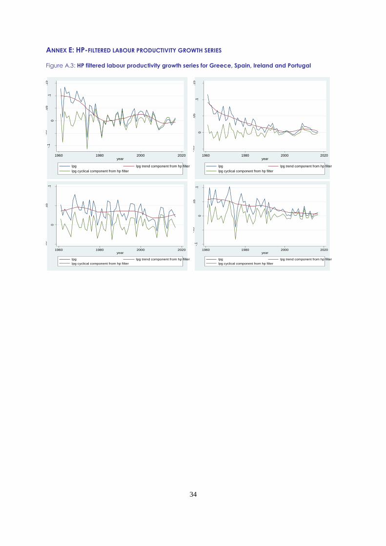
and wage adjustment based on trend labour productivity growth (S2), we employ a Hodrick-Prescott

filter to obtain trend labour productivity growth with a smoothing parameter of 100. Results are shown

in Figure A.3 in Annex E. The resulting series are used to compute the wage indicator in this scenario

and the Kalman filter approach is used to estimate the NAWRU.

3.2. ECONOMETRIC APPROACH

The NAWRU is determined by an unobserved component model, which is estimated by a bi-variate

Kalman filter using ECFIN's GAP software (Planas and Rossi 2009). This econometric model include

the Phillips curve specified in equation (2.16) and (2.16`) respectively as well as an equation that

assumes a second order auto-regressive process for the cyclical term of the unemployment rate (the

5 http://ec.europa.eu/economy_finance/db_indicators/ameco/index_en.htm

6 http://ec.europa.eu/economy_finance/eu/forecasts/index_en.htm

http://ec.europa.eu/economy_finance/db_indicators/ameco/index_en.htm

http://ec.europa.eu/economy_finance/eu/forecasts/index_en.htm

14

unemployment gap) and a second order random walk for the trend component (the NAWRU). The

econometric equation for the TKP7 and the NKP take the respective forms:

Δ𝜋𝑡𝑤 − Δ𝑔𝑦𝑙𝑡 = −𝛽(𝑢𝑡 − 𝑢𝑡

∗) + 휀𝑡𝑇𝐾𝑃𝐶 (3.1)

𝜋𝑡𝑤 − 𝜋𝑡

𝑝− 𝑔𝑦𝑙𝑡 = 𝛽0(𝜋𝑡−1

𝑤 − 𝜋𝑡−1𝑝

− 𝑔𝑦𝑙𝑡−1) − 𝛽1(𝑢𝑡 − 𝑢𝑡∗) + 𝛽2(𝑢𝑡−1 − 𝑢𝑡−1

∗ ) + 휀𝑡𝑁𝐾𝑃𝐶 (3.2)

The model for unemployment takes the form:

𝑢𝑡 = 𝑐𝑡 + 𝑛𝑡 (3.3)

𝑐𝑡 = 𝛿1𝑐𝑡−1 + 𝛿2𝑐𝑡−2 + 휀𝑡𝑐 (3.4)

𝑛𝑡 = 𝛾𝑡−1 + 𝑛𝑡−1 + 휀𝑡𝑛 (3.5)

𝛾𝑡−1 = 𝛾𝑡−2 + 휀𝑡𝛾 (3.6)

For a more detailed description of the estimation method of the NAWRU applied here see Havik et al.

(2014) and Planas and Rossi (2009).

4. EMPIRICAL RESULTS

In this section we compare NAWRU estimates based on the NKP model to those based on the TKP

model. For the NKP model we study both the baseline scenario (S1) and the scenario with real wage

rigidities (RWR) (S2). Key insights of this comparison are that the NKP model yields less pro-cyclical

NAWRU estimates during severe recessions and that the fit of the wage Phillips curve improves as

well as the significance of the link between labour market slack and labour cost developments when

relying on the NKP approach.

Figures 4.1–4.4 show that NAWRUs based on the NKP model are slightly less pro-cyclical than those

based on the TKP model, around the time of the recent crisis, in the case of Greece, Ireland and most

notably Spain. In the case of Portugal, it is less apparent that NKP-based NAWRUs are less pro-

cyclical. Nevertheless, for that country the NKP model appears to yield estimates for the NAWRU that

are, overall, smoother.

Tables at the bottom of Figures 4.1–4.4 show that the fit of the wage Phillips curve improves when

relying on the NKP model in all cases, except for Greece. Moreover, the t-statistic of the coefficient on

the unemployment gap (β1) is higher in absolute terms in the NKP model in all cases, suggesting that

this model identifies a stronger link between labour market slack and labour cost developments.

Adding real-wage rigidities to the NKP model, by allowing wages to adjust to trend rather than actual

labour productivity (i.e. scenario S2), the t-statistic on the β1 and the fit of the wage Phillips curve

further improves in all cases. In particular in Ireland, the results improve notably and the NAWRU

displays a less pro-cyclical pattern as recent declines in the labour cost indicator are better tracked by

the model than in the case of the TKP or the NKP without real wage rigidities. Noteworthy, the labour

7 For a derivation of the TKP, see for example Blanchard and Katz (1999).

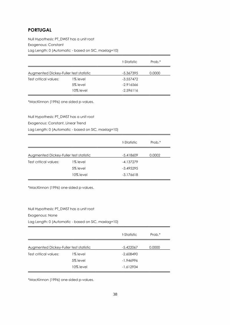
15

cost indicator in the NKP model with real wage rigidities may be non-stationary, as one of its

components is a trend variable. Annex F reports unit root test results which however indicate that the

Null hypothesis of a unit root can be rejected in all cases.

To build intuition, note that the NAWRU estimates based on the NKP and the TKP model differ when

nominal wages fall strongly while price development display some inertia, a situation which

characterised developments in Spain, for instance, in the aftermath of the crisis. Under such

circumstances, real unit labour cost growth (the NKP labour cost indicator) declines more strongly

(and persistently) than the change in the nominal unit labour cost (the TKP labour cost indicator). As

such, the NKP model identifies a larger (and more persistent) unemployment gap and posts a less pro-

cyclical NAWRU. To illustrate, note that in Spain, after 2009, the change in the nominal unit labour

cost rapidly reverted back to zero, while real unit labour cost growth posted a more protracted negative

dynamic, pointing at larger and more persistent slack in the Spanish labour market. In turn, the NKP

based NAWRU estimate for Spain reached 22% by 2015, compared to 26.4% for the TKP based

estimate.

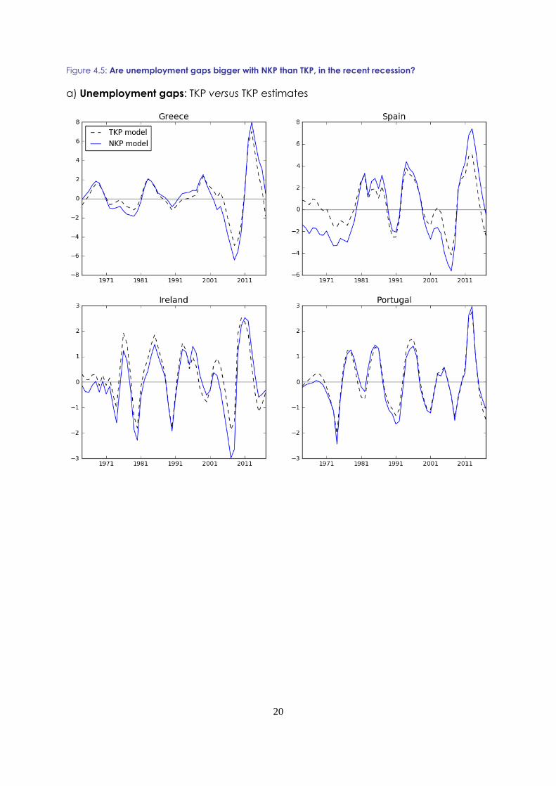
Figure 5 highlights comparison across the TKP and the NKP in terms of unemployment gap. As TKP

based NAWRUs tend to be excessively pro-cyclical in times of crisis, that model also yields narrower

unemployment gaps under such circumstances. This is the case for all countries, except Portugal. Yet

when adding the real wage rigidity to the NKP model (i.e. scenario S2) the same is also observed for

Portugal. The latter suggests that adding rigidities may further improve accuracy of trend-cycle

decomposition, especially in volatile times where such rigidities become more binding.

Overall, as the two labour cost indicators appear to diverge only occasionally, the choice of the model

bears consequences only during volatile times. In all countries, the two models tended to yield similar

NAWRUs before the crisis. This suggests the two labour cost indicators differ notably only in times of

large labour market adjustments. As such, the use of the NKP approach provides some insurance

against the risk of reporting upwardly biased NAWRU estimates in times of crisis while adding more

rigidities such as real wage rigidities, may provide additional robustness against, as results for Portugal

suggest.

In sum, evidence reported in this section suggests that, compared to the TKP, the NKP yields a better

fit for the wage Phillips curve and a stronger link between the labour slack and the labour cost

indicator and offers some insurance against risks of NAWRU over-estimation in times of crisis. These

results suggest that the NKP model (with real wage rigidities) provides a valuable alternative to the

commonly used TKP model for analysis of the labour market in terms of trend-cycle decomposition.

Note that to assess the merit of switching to the NKP model for real-time analysis would require

checking the degree to which its NAWRU estimates are prone to revisions. While the NKP appears to

be better at “getting the story right” than the TKP, if it were prone to larger NAWRU revisions than

the TKP this would undermine its use in real-time. Checking this is beyond the scope of this paper. It

would require assessing whether and at what horizon NKP based NAWRU estimates are more

unstable than TKP based ones. Whether the benefits the NKP model yields in terms of accuracy of the

trend-cycle decomposition are at the expense of relative stability of NAWRU estimates is an issue

worth investigating in future work to assess its use for real-time analysis.

16

Figure 4.1: NAWRU and fit of the Phillips curve—TKP versus NKP8

GREECE

Notes: Labour cost indicator across the models: (a) 2nd difference of NULC; (b) 1st difference of RULC; (c) 1st

difference of RULC computed using trend productivity.

TKP NKP NKP-RWR

Coefficient estimates

(t-statistics in brackets)

(**) if restricted

UB or LB if (upper or lower) bound reached

β1: -0.20

(-0.6052)

β1: -0.35

(-0.8696)

β2: 0.28 (**)

β1: -0.56

(-1.2354)

β2: 0.57

(1.2790)

R2 0.1263 0.1150 0.1223

8 Note that the variance bounds for Greece for the TKP model were taken from the Winter 2014 forecasting exercise as it was

the last exercise based on the TKP model.

17

Figure 4.2: NAWRU and fit of the Phillips curve—TKP versus NKP

SPAIN



TKP NKP NKP-RWR



(**) if restricted


β1: -0.29

(-1.7412)

β1: -0.36

(-2.1699)

β2: 0.19 (**)

β1: -0.28

(-2.3826)

β2: 0.00 (LB)

R2 0.1821 0.2268 0.2148

18


IRELAND



TKP NKP NKP-RWR



(**) if restricted


β1: -0.74

(-1.5215)

β1: -0.87

(-2.0743)

β2: 0.43 (**)

β1: -0.59

(-2.7605)

β2: 0.00 (LB)

R2 0.1527 0.1795 0.2426

19


PORTUGAL



TKP NKP NKP-RWR



(**) if restricted


β1:-0.89

(-1.4059)

β1:-1.37

(-1.9435)

β2: 0.74 (**)

β1: -1.64

(-2.3959)

β2: 0.79

(1.1623)

R2 0.0872 0.1874 0.1400

20

Figure 4.5: Are unemployment gaps bigger with NKP than TKP, in the recent recession?

a) Unemployment gaps: TKP versus TKP estimates

21

Figure 4.5 (continued)

b) Unemployment gaps: NKP/real wage rigidity versus TKP estimates

22

5. CONCLUSION

In this paper we argue that non-cyclical unemployment estimates based on a traditional

(accelerationist) Phillips curve risk being too pro-cyclical, due to inadequate treatment of price

expectations, an issue likely to matter particularly in times of large labour market adjustments, such as

around crisis episodes. In turn, we argue that the New-Keynesian Phillips curve provides a remedy, by

providing better treatment for price rigidities, which, as we show, can be inferred from theory.

To assess this empirically, we compare non-cyclical unemployment estimates based, respectively, on

the accelerationist Phillips curve and the New-Keynesian Wage Phillips curve. We provide estimates

for four crisis-hit EU member states (Greece, Spain, Ireland and Portugal) that underwent major

swings in the unemployment rate, in recent years. Our results confirm that the New-Keynesian Wage

Phillips curve yields less pro-cyclical estimates of the non-cyclical part of unemployment for those

countries during the crisis. The empirical fit also improves when using the New-Keynesian Wage

Phillips curve. Additionally, augmenting the New-Keynesian Wage Phillips curve to reflect the impact

of real wage rigidities further improves the fit, pointing at further improvement in the extraction of the

cyclical component of unemployment.

The practical interpretation of these results is that the change in nominal unit labour cost growth, the

indicator suggested by the accelerationist Phillips curve to identify the unemployment gap, provides a

poor signal in volatile times. Instead, the real unit labour cost growth, which is the indicator suggested

by the New-Keynesian Wage Phillips curve, is a better indicator of labour market slack, under such

circumstances.

Our analysis generally contributes to the vast literature documenting the empirical relevance the New-

Keynesian (Wage) Phillips curve, with particular focus on the euro area. This analysis points at the

importance of accounting properly for various rigidities that, in particular, drive price and wage

developments. In times of large labour market adjustment, adequately accounting for those aspects

appears key to support Phillips curve based trend-cycle decomposition of unemployment

developments. Evidence that accounting for real wage rigidities further improves results, confirm the

merit of seeking to model additional rigidities in frameworks that underpin empirical Phillips curve

specifications. Both theoretical and empirical results presented here suggest that nominal and real

wage rigidities are not the only sources of variation of the equilibrium unemployment rate. In

particular, our New-Keynesian Wage Phillips curve estimates remain noisy, pointing at the need to

further enrich the underlying model (e.g. labour demand frictions). Recalling the important theoretical

and empirical differences across alternative Phillips curve models, as highlighted in this paper, is also

warranted when debating the performance of model from a practical perspective.

From a policy perspective, the illustrated risk of reporting biased NAWRU estimates when relying on

traditional Phillips curve approaches is unsettling. Evidence suggests the bias would be most severe in

times of crisis, when accurate assessment is arguably most needed. In the EU context, NAWRU

estimates also feed into potential output calculations which, in turn, affect computation of cyclically-

adjusted fiscal variables used to underpin the EU fiscal surveillance framework. Hence, the reporting

of biased NAWRU estimates has far reaching implications from a policy perspective, pointing at the

merit of further investigating the apparent merit of relying on NKP models featuring all relevant

rigidities, rather than relying on the commonly used TKP approach.

23

6. REFERENCES

Alstadheim, R. (2013). How New Keynesian is the US Phillips curve? Working Paper

2013/25, Norges Bank.

Bardsen, G., Jansen, E. S., and Nymoen, R. (2004). Econometric evaluation of the new

keynesian phillips curve*. Oxford Bulletin of Economics and Statistics, 66:671-686.

Blanchard, O. and Galí, J. (2007): Real wage rigidities and the New-Keynesian model,

Journal of Money, Credit and Banking, 39: 35–65.

Blanchard, O. and Katz, L.F. (1999): Wage dynamics: reconciling theory and evidence,

American Economic Review 89, pp. 69-74.

Calvo, G. (1983): Staggered Contracts in a Utility-Maximizing Framework, Journal of

Monetary Economics 12, pp. 383–398.

Fuhrer, J. and Moore, G. (1995). Inflation persistence. The Quarterly Journal of Economics,

110(1):127-159.

Galí, J. (2011): The Return of the Wage-Phillips-curve, Journal of the European Economic

Association, 9(3):436–461.

Galí, J. and Gertler, M. (1999). Inflation dynamics: A structural econometric analysis. Journal

of Monetary Economics, 44(2):195-222.

Galí, J., Gertler, M., and Lopez-Salido, J. D. (2001). European inflation dynamics. European

Economic Review, 45(7):1237-1270.

Galí, J., Gertler, M., and David Lopez-Salido, J. (2005). Robustness of the estimates of the

hybrid New Keynesian Phillips curve. Journal of Monetary Economics, 52(6):1107-1118.

Gerchert, S., K. Rietzler and S. Tober (2015): The European Commission's new NAIRU:

Does it deliver?, Applied Economic Letters, 2015.

Havik, K., K. McMorrow, F. Orlandi, C. Planas, R. Raciborski, W. Roeger, A. Rossi, A.

Thum-Thysen and V. Vandermeulen (2014): The Production Function Methodology for

Calculating Potential Growth Rates and Output Gaps, European Economic Papers, Nr. 535.

Hondroyiannis, G., Swamy, P., and Tavlas, G. S. (2008). Inflation dynamics in the euro area

and in new EU members: Implications for monetary policy. Economic Modelling,

25(6):1116-1127.

Jondeau, E. and Bihan, H. L. (2005). Testing for the new Keynesian Phillips curve: additional

international evidence. Economic Modelling, 22(3):521-550.

López-Pérez, V. (2016). Do professional forecasters behave as if they believed in the new

keynesian phillips curve for the euro area? Empirica, pages 1-28.

24

Mavroeidis, S. (2005). Identification Issues in Forward-Looking Models Estimated by GMM,

with an Application to the Phillips Curve. Journal of Money, Credit and Banking, 37(3):421-

48.

Mavroeidis, S. (2006). Testing the New Keynesian Phillips Curve Without Assuming

Identification. Technical report.

Mazumder, S. (2012). European inflation and the new Keynesian Phillips curve. Southern

Economic Journal, 79(2):322-349.

Paloviita, M. (2006). Inflation Dynamics in the Euro Area and the Role of Expectations.

Empirical Economics, 31(4):847-860.

Planas, C. and A. Rossi (2009): Program GAP. Technical Description and User-manual, JRC

Scientific and Technical Research series – ISSN 1018-5593, Luxemburg.

Roberts, J. M. (1995). New Keynesian Economics and the Phillips Curve. Journal of Money,

Credit and Banking, 27(4):975-84.

Rotemberg, J. (1982): Sticky Prices in the United States, Journal of the Political Economy 90,

pp. 1187–1211.

Rudd, J. and Whelan, K. (2005). New tests of the new-Keynesian Phillips curve. Journal of

Monetary Economics, 52(6):1167-1181.

Rumler, F. (2007). Estimates of the open economy new Keynesian Phillips curve for euro area

countries. Open Economies Review, 18(4):427-451.

Sbordone, A. M. (2002). Prices and unit labour costs: a new test of price stickiness. Journal of

Monetary Economics, 49(2):265-292.

Stock, J. H., Wright, J. H., and Yogo, M. (2002). A Survey of Weak Instruments and Weak

Identification in Generalized Method of Moments. Journal of Business & Economic Statistics,

20(4):518-29.

Tillmann, P. (2009). The New Keynesian Phillips curve in Europe: does it fit or does it fail?

Empirical Economics, 37(3):463-473.

Vogel, L. (2008). The Relationship between the Hybrid New Keynesian Phillips Curve and

the NAIRU over Time. Macroeconomics and Finance Series 200803, Hamburg University,

Department Wirtschaft und Politik.

25

7. ANNEX

ANNEX A: UNEMPLOYMENT RATES AND NAWRUS ACROSS EU MEMBER STATES

Figure A.1: Percentage point change between 2008 and 2012 in the unemployment rate across EU

member states


Figure A.2: Percentage point change between 2008 and 2012 in the NAWRU across EU member states


26

ANNEX B: DETAILED DERIVATION OF THE PHILLIPS CURVE

Nominal rigidities

To solve the optimisation problem in section 2, define the Lagrangian as:

ℒ𝑡 ≡ 𝐸𝑡(∑ 𝛽𝑗𝑈𝑡+𝑗∞𝑗=0 − ∑ 𝛽𝑗𝜆𝑡+𝑗𝐵𝐶𝑡+𝑗

∞𝑗=0 ) (B.1)

The first order conditions are:

𝜕ℒ

𝜕𝐵𝑡= 0 ⟺ 𝜆𝑡 = 𝐸𝑡𝜆𝑡+1𝛽(1 + 𝑟𝑡) (B.2)

𝜕ℒ

𝜕𝐶𝑡= 0 ⟺ 𝑢𝐶𝑡

= 𝜆𝑡 =1

𝐶𝑡 (B.3)

𝜕ℒ

𝜕𝑤𝑡(𝑖)= 0 ⟺ 𝑢𝐿𝑡(𝑖)

(−𝜃)𝑊𝑡(𝑖)−𝜃−1 𝐿𝑡

𝑊𝑡−𝜃 + 𝜆𝑡

(1−𝜃)𝑊𝑡(𝑖)

𝑃𝑡

−𝜃 𝐿𝑡

𝑤𝑡−𝜃

− 𝜆𝑡𝛾 [𝑊𝑡(𝑖)

Π𝑡𝑊(𝑖)𝑡−1−

1]𝑤𝑡𝐿𝑡

𝑝𝑡(

1

Π𝑡𝑤(𝑖)𝑡−1) + 𝐸𝑡 (𝜆𝑡+1𝛽𝛾 [

𝑤𝑡+1(𝑖)

Π𝑡+1𝑤(𝑖)𝑡− 1]

𝑤𝑡+1𝐿𝑡+1

𝑝𝑡+1(

𝑤𝑡+1(𝑖)

Π𝑡+1(𝑤(𝑖)𝑡)2)) = 0

(B.4a)

Assume symmetry: 𝑊𝑡 = 𝑊𝑡(𝑖) and therefore 𝐿𝑡 = 𝐿𝑡(𝑖)

𝑢𝐿𝑡(−𝜃)

𝐿𝑡

𝑊𝑡+ 𝜆𝑡

(1−𝜃)𝐿𝑡

𝑃𝑡 − 𝜆𝑡𝛾 [

𝑊𝑡

Π𝑡𝑊𝑡−1− 1]

𝑊𝑡𝐿𝑡

𝑃𝑡(

1

Π𝑡𝑊𝑡−1) + 𝐸𝑡 (𝜆𝑡+1𝛽𝛾 [

𝑤𝑡+1

Π𝑡+1𝑤𝑡−

1]𝑤𝑡+1𝐿𝑡+1

𝑝𝑡+1(

𝑤𝑡+1

Π𝑡+1𝑤𝑡2)) = 0 (B.4.b)

Rearranging yields:9

−𝑢𝐿𝑡(−𝜃) =

𝜆𝑡𝑊𝑡

𝑃𝑡 ((1 − 𝜃) − 𝛾 [

𝑊𝑡

Π𝑡𝑊𝑡−1− 1] (

𝑊𝑡

Π𝑡𝑊𝑡−1) + 𝐸𝑡 (

𝛽𝜆𝑡+1

𝜆𝑡𝛾 [

𝑊𝑡+1

Π𝑡+1𝑊𝑡− 1] (

𝑊𝑡+1

Π𝑡+1𝑊𝑡 )))

(B.4.c)

Equation (B.4.c) is not linear in adjustment costs so we perform a first order Taylor

approximation of 𝛾 [𝑊𝑡

Π𝑡𝑊𝑡−1− 1] (

𝑊𝑡

Π𝑡𝑊𝑡−1) around the steady state.

To this purpose we define

Ψt =𝑊𝑡

Π𝑡𝑊𝑡−1 and consequently 𝑓(Ψ𝑡) = 𝛾(Ψ𝑡 − 1)Ψ𝑡

In the steady state we have

𝑊𝑡

Π𝑡𝑊𝑡−1=

𝑊𝑡+1

Π𝑡𝑊𝑡 = 1 and Π𝑡 = Π = 1 and consequently Ψ = 1

9 Assuming

𝑊𝑡+1𝐿𝑡+1

𝑃𝑡+1𝐿𝑡≈

𝑊𝑡

𝑃𝑡.

27

The Taylor approximation of 𝑓(Ψ𝑡) is

𝑓(Ψ𝑡) ≈ 𝑓(Ψ) + 𝑓′(Ψ)(Ψ𝑡 − Ψ)

with

𝑓′(Ψt) = 𝛾Ψ𝑡 + 𝛾(Ψt − 1) = 𝛾(2Ψt − 1) and 𝑓′(Ψ) = 𝛾

So

𝑓(Ψ𝑡) ≈ 𝛾(Ψ𝑡 − 1)

Then, using 𝑢𝐿𝑡= −χ𝐿𝑡

𝜂, equations (B.2-B.3) and the Taylor approximation above and

assuming a constant discount factor 𝛽 =1

1+𝑟𝑡 or no consumption fluctuations 𝐸𝑡

𝜆𝑡

𝜆𝑡+1 =

𝐸𝑡𝐶𝑡+1

𝐶𝑡= 1, we can rewrite equation (B.4.c) as

𝜒𝐿𝑡𝜂(−𝜃) =

1

𝐶𝑡

𝑊𝑡

𝑃𝑡 ((1 − 𝜃) − 𝛾(Ψ𝑡 − 1) + 𝛽𝛾(𝐸𝑡Ψ𝑡+1 − 1)) (B.4.d)

Simplifying and defining 𝜓𝑡 = Ψ𝑡 − 1, we can rewrite equation (2.8.e) as

𝜒𝐿𝑡𝜂(−𝜃) =

1

𝐶𝑡

𝑊𝑡

𝑃𝑡 ((1 − 𝜃) − 𝛾𝜓𝑡 + 𝛽𝛾𝐸𝑡𝜓𝑡+1)

Further, rearranging and defining (1 + 𝑚𝑢𝑝𝑡𝑤) =

𝜃

𝜃−1=

(−𝜃)

(1−𝜃) we can write

(−𝜃)𝜒𝐿𝑡𝜂𝐶𝑡

(1−𝜃)=

𝑊𝑡

𝑃𝑡(1 +

𝛾

(1−𝜃)(𝛽𝐸𝑡𝜓𝑡+1 − 𝜓𝑡))

(−𝜃)𝜒𝐿𝑡𝜂𝐶𝑡

(1−𝜃)=

𝑊𝑡

𝑃𝑡(1 −

𝛾

(𝜃−1)(𝛽𝐸𝑡𝜓𝑡+1 − 𝜓𝑡))

Define 𝑊𝑡𝑟 =

𝑊𝑡

𝑃𝑡 and rewrite

𝑊𝑡𝑟 =


𝜂𝐶𝑡

(1−𝛾


(B.4.d)

Or alternatively as labour supply equation

𝐿𝑡 = (𝑊𝑡

𝑟(1−𝛾


𝜒𝐶𝑡(1+𝑚𝑢𝑝𝑡𝑤)

)

1/𝜂

(B.4.e)

This relationship can also be used to determine the labour force, namely as the number of

workers which are indifferent between working and not working

𝐿𝐹𝑡 = (𝑊𝑡

𝑟

𝜒𝐶𝑡)1/𝜂

(B.5)

28

The cyclically adjusted employment rate (the employment rate in the absence of wage

adjustment costs) is given by

𝐿𝐶𝐴𝑡 = (𝑊𝑡

𝑟


)1/𝜂

(B.6)

And the cyclically adjusted unemployment rate is given by

𝐿𝐹𝑡

𝐿𝐶𝐴𝑡= (1 + 𝑢𝑡

∗) = (1 + 𝑚𝑢𝑝𝑡𝑤)

1

𝜂 (B.7)

The actual unemployment rate

𝐿𝐹𝑡

𝐿𝑡= (1 + 𝑢𝑡 ) = (

(1+𝑚𝑢𝑝𝑡𝑤)

(1−𝛾


)

1

𝜂

(B.8)10

Substituting equation (B.7) into (B.8) yields

(1 + 𝑢𝑡 ) = (1 + 𝑢𝑡∗) (

1

(1−𝛾


)

1

𝜂

(B.9)

1 −𝛾

(𝜃−1)(𝛽𝐸𝑡𝜓𝑡+1 − 𝜓𝑡) = [

(1+𝑢𝑡)

(1+𝑢𝑡∗)]−𝜂

Taking logs yields

−𝛾

(𝜃−1)(𝛽𝐸𝑡𝜓𝑡+1 − 𝜓𝑡) = −𝜂 ln [

(1+𝑢𝑡)

(1+𝑢𝑡∗)]

−𝛾

(𝜃−1)(𝛽𝐸𝑡𝜓𝑡+1 − 𝜓𝑡) = −𝜂(ln(1 + 𝑢𝑡) − ln(1 + 𝑢𝑡

∗))

−𝛾

(𝜃−1)(𝛽𝐸𝑡𝜓𝑡+1 − 𝜓𝑡) = −𝜂(𝑢𝑡 − 𝑢𝑡

∗)

𝜓𝑡 = 𝛽𝐸𝑡𝜓𝑡+1 −𝜂(𝜃−1)


∗) (B.10)

Real wage rigidities

Rewrite equation (B.4.e) by adding a term reflecting dependence on past real wages (real

wage rigidity) – in addition to labour and consumption, wages are adjusting sluggishly to past

real wages (corrected for the productivity growth trend) – as below. Note that in this section

we assume that 𝜓𝑡 = 𝜋𝑡𝑤 − 𝜋𝑡

𝑝 − 𝑔𝑦𝑙𝑡𝑇 .

𝑊𝑡𝑟 = [

𝜒𝐿𝑡𝜂𝐶𝑡(1+𝑚𝑢𝑝𝑡

𝑤)

(1−𝛾

(𝜃−1)(𝛽𝐸𝑡𝜓𝑡+1−𝜓𝑡)

]

1−𝜙

[𝑊𝑡−1𝑟 (1 + 𝑔𝑌𝐿𝑇

𝑡)]𝜙 (B.4.d')

10

In approximation around the steady state this expression can also be written as

𝐿𝐹𝑡

𝐿𝑡= (1 + 𝑢𝑡 ) = (

1

(1−𝛾

(𝜃−1)(𝛽𝐸𝑡𝜓𝑡+1−𝜓𝑡))(1−𝑚𝑢𝑝𝑡

𝑤))

1

𝜂

29

Rearranging and solving for 𝐿𝑡 yields

𝑊𝑡𝑟

11−𝜙

𝑊𝑡−1𝑟

−𝜙1−𝜙

(1 + 𝑔𝑌𝐿𝑇𝑡)

−𝜙

1−𝜙 =𝜒𝐿𝑡

𝜂𝐶𝑡(1+𝑚𝑢𝑝𝑡

𝑤)

(1−𝛾


𝐿𝑡 = [𝑊𝑡𝑟

11−𝜙

𝑊𝑡−1𝑟

−𝜙1−𝜙

(1 + 𝑔𝑌𝐿𝑇𝑡)

−𝜙

1−𝜙(1−

𝛾



]

1/𝜂

(B.4.e')

Divide equation (B.5) by (B.4e') to determine the unemployment rate as a function of those

who are unemployed due to frictions in the labour market and full employment under now

frictions:

𝐿𝐹𝑡

𝐿𝑡= (1 + 𝑢𝑡) =

[

𝑊𝑡𝑟

𝜒𝐶𝑡

𝑊𝑡𝑟

11−𝜙

𝑊𝑡−1𝑟

−𝜙1−𝜙

(1+𝑔𝑌𝐿𝑇𝑡)

−𝜙1−𝜙(1−

𝛾(𝜃−1)

(𝛽𝐸𝑡𝜓𝑡+1−𝜓𝑡))

𝜒𝐶𝑡(1+𝑚𝑢𝑝𝑡𝑤) ]

1/𝜂

𝐿𝐹𝑡

𝐿𝑡= [


𝑊𝑡𝑟

𝜙1−𝜙

𝑊𝑡−1𝑟

−𝜙1−𝜙

(1+𝑔𝑌𝐿𝑇𝑡)

−𝜙1−𝜙(1−

𝛾


]

1/𝜂

𝐿𝐹𝑡

𝐿𝑡=

[


[𝑊𝑡

𝑟

(1+𝑔𝑌𝐿𝑇𝑡)𝑊𝑡−1

𝑟 ]

𝜙1−𝜙

(1−𝛾

(𝜃−1)(𝛽𝐸𝑡𝜓𝑡+1−𝜓𝑡))]

1/𝜂

(B.8')

Where

𝑊𝑡𝑟

(1+𝑔𝑌𝐿𝑇𝑡)𝑊𝑡−1

𝑟 =

𝑊𝑡𝑃𝑡

(𝑊𝑡−1𝑃𝑡−1

)(𝑌𝐿𝑡

𝑌𝐿𝑡−1)𝑇 =

𝑊𝑡𝑃𝑡

(𝐿𝑡𝑌𝑡

)𝑇

(𝑊𝑡−1𝑃𝑡−1

)(𝐿𝑡−1𝑌𝑡−1

)𝑇 = 1 + (𝜋𝑡

𝑤 − 𝜋𝑡𝑝 − 𝑔𝑦𝑙𝑡

𝑇) = 1 + 𝜓𝑡

Using equation (B.7) we can write equation (B.8') as

(1+𝑢𝑡)

(1+𝑢𝑡∗)

= [1

[1+𝜓𝑡]𝜙

1−𝜙(1−𝛾


]

1/𝜂

(B.9')

1 −𝛾

(𝜃−1)(𝛽𝐸𝑡𝜓𝑡+1 − 𝜓𝑡) = [

(1+𝑢𝑡)

(1+𝑢𝑡∗)]−𝜂

1

[1+𝜓𝑡]𝜙

1−𝜙

1 −𝛾

(𝜃−1)(𝛽𝐸𝑡𝜓𝑡+1 − 𝜓𝑡) = [

(1+𝑢𝑡)

(1+𝑢𝑡∗)]−𝜂

1

[1+𝜓𝑡]𝜙

1−𝜙

Taking logs yields

−𝛾

(𝜃−1)(𝛽𝐸𝑡𝜓𝑡+1 − 𝜓𝑡) = −𝜂 ln [

(1+𝑢𝑡)

(1+𝑢𝑡∗)] + ln [[1 + 𝜓𝑡]

−𝜙

1−𝜙]

30

−𝛾

(𝜃−1)(𝛽𝐸𝑡𝜓𝑡+1 − 𝜓𝑡) = −𝜂(ln(1 + 𝑢𝑡) − ln(1 + 𝑢𝑡

∗)) −𝜙

1−𝜙ln(1 + 𝜓𝑡)

−𝛾

(𝜃−1)(𝛽𝐸𝑡𝜓𝑡+1 − 𝜓𝑡) = −𝜂(𝑢𝑡 − 𝑢𝑡

∗) −𝜙

1−𝜙𝜓𝑡

𝜓𝑡 = 𝛽𝐸𝑡𝜓𝑡+1 −(𝜃−1)

𝛾

𝜙

1−𝜙𝜓𝑡 −

𝜂(𝜃−1)


∗)

(1 +(𝜃−1)

𝛾

𝜙

1−𝜙)𝜓𝑡 = 𝛽𝐸𝑡𝜓𝑡+1 −

𝜂(𝜃−1)


∗)

Based on equation (B.9') we can rewrite the Phillips curve as

𝜓𝑡 =𝛽

(1+(𝜃−1)

𝛾

𝜙


𝜂(𝜃−1)

𝛾(1+(𝜃−1)

𝛾

𝜙


∗) (B.10')

31

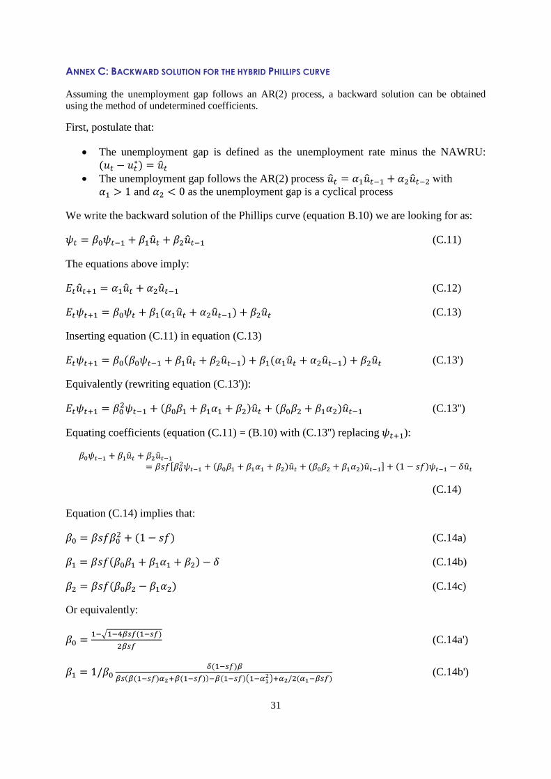
ANNEX C: BACKWARD SOLUTION FOR THE HYBRID PHILLIPS CURVE

Assuming the unemployment gap follows an AR(2) process, a backward solution can be obtained

using the method of undetermined coefficients.

First, postulate that:

The unemployment gap is defined as the unemployment rate minus the NAWRU:

(𝑢𝑡 − 𝑢𝑡∗) = �̂�𝑡

The unemployment gap follows the AR(2) process �̂�𝑡 = 𝛼1�̂�𝑡−1 + 𝛼2�̂�𝑡−2 with

𝛼1 > 1 and 𝛼2 < 0 as the unemployment gap is a cyclical process

We write the backward solution of the Phillips curve (equation B.10) we are looking for as:

𝜓𝑡 = 𝛽0𝜓𝑡−1 + 𝛽1�̂�𝑡 + 𝛽2�̂�𝑡−1 (C.11)

The equations above imply:

𝐸𝑡�̂�𝑡+1 = 𝛼1�̂�𝑡 + 𝛼2�̂�𝑡−1 (C.12)

𝐸𝑡𝜓𝑡+1 = 𝛽0𝜓𝑡 + 𝛽1(𝛼1�̂�𝑡 + 𝛼2�̂�𝑡−1) + 𝛽2�̂�𝑡 (C.13)

Inserting equation (C.11) in equation (C.13)

𝐸𝑡𝜓𝑡+1 = 𝛽0(𝛽0𝜓𝑡−1 + 𝛽1�̂�𝑡 + 𝛽2�̂�𝑡−1) + 𝛽1(𝛼1�̂�𝑡 + 𝛼2�̂�𝑡−1) + 𝛽2�̂�𝑡 (C.13')

Equivalently (rewriting equation (C.13')):

𝐸𝑡𝜓𝑡+1 = 𝛽02𝜓𝑡−1 + (𝛽0𝛽1 + 𝛽1𝛼1 + 𝛽2)�̂�𝑡 + (𝛽0𝛽2 + 𝛽1𝛼2)�̂�𝑡−1 (C.13'')

Equating coefficients (equation (C.11) = (B.10) with (C.13'') replacing 𝜓𝑡+1):

𝛽0𝜓𝑡−1 + 𝛽1�̂�𝑡 + 𝛽2�̂�𝑡−1

= 𝛽𝑠𝑓[𝛽02𝜓𝑡−1 + (𝛽0𝛽1 + 𝛽1𝛼1 + 𝛽2)�̂�𝑡 + (𝛽0𝛽2 + 𝛽1𝛼2)�̂�𝑡−1] + (1 − 𝑠𝑓)𝜓𝑡−1 − 𝛿�̂�𝑡

(C.14)

Equation (C.14) implies that:

𝛽0 = 𝛽𝑠𝑓𝛽02 + (1 − 𝑠𝑓) (C.14a)

𝛽1 = 𝛽𝑠𝑓(𝛽0𝛽1 + 𝛽1𝛼1 + 𝛽2) − 𝛿 (C.14b)

𝛽2 = 𝛽𝑠𝑓(𝛽0𝛽2 − 𝛽1𝛼2) (C.14c)

Or equivalently:

𝛽0 =1−√1−4𝛽𝑠𝑓(1−𝑠𝑓)

2𝛽𝑠𝑓 (C.14a')

𝛽1 = 1/𝛽0 𝛿(1−𝑠𝑓)𝛽

𝛽𝑠(𝛽(1−𝑠𝑓)𝛼2+𝛽(1−𝑠𝑓))−𝛽(1−𝑠𝑓)(1−𝛼12)+𝛼2/2(𝛼1−𝛽𝑠𝑓)

(C.14b')

32

𝛽2 =𝛽𝑠𝑓𝛼2

1−𝛽𝑠𝑓𝛽0𝛽1 (C.14c')

with 𝛼1 > 0 and 𝛼2 < 0

Note, from (C.14a) one can derive the share of forward looking wage setters from the estimate

of 𝛽0.

Note also that (C.14c') implies that the lagged unemployment gap has a positive effect on the

wage indicator in period t. This is due to the cyclicality of the unemployment gap. A negative

unemployment gap in t-1 is signalling a positive gap in t+1 and since wages are set in period t

with an expectation about cyclical conditions in t+1, a negative unemployment gap in t+1

predicts a wage increase in period t.

How does real wage rigidity modify the backward solution?

The wage Phillips curve with and without real wage rigidity differs essentially by the

coefficient of the wage expectation term. Without real wage rigidity this term is equal to the

discount factor and is constrained to a value slightly below 1.

𝜓𝑡 = 𝛽𝐸𝑡𝜓𝑡+1 −𝜂(𝜃−1)


∗) (C.15)

In contrast, with real wage rigidity, the coefficient in front of the wage expectation term can

become arbitrarily small as the degree of real wage rigidity becomes large (𝜙 → 1).

𝜓𝑡 =𝛽

(1+(𝜃−1)

𝛾

𝜙


𝜂(𝜃−1)

𝛾(1+(𝜃−1)

𝛾

𝜙


∗)

This relaxes the parameter constraint (C.14c') to

𝛽2 =𝛽∗𝑠𝑓𝛼2

1−𝛽𝑠𝑓𝛽0𝛽1 where 𝛽∗ =

𝛽

(1+(𝜃−1)

𝛾

𝜙

1−𝜙) (C.14c'')

And 𝛽∗ becomes a free parameter with 0 < 𝛽∗ < 1. Thus, real wage rigidity imposes the

constraint

𝛽2 > 0

on the backward solution.

33

ANNEX D: COMPARISON WITH WAGE PHILLIPS CURVE DERIVED UNDER CALVO WAGE SETTING

J. Galí (2011) presented a paper where he derived a wage Phillips curve in a Calvo wage

setting framework. The Calvo framework is attractive since it allows to microfound the wage

setting process in terms of (expected) contract length and specific wage indexation schemes

(for those wage setters which are not able to renegotiate wages in the current period).

Galí makes a number of assumptions, which need to be taken into account when comparing

his Phillips curve to ours. Galí assumes that, for workers that cannot optimise in the current

period, wages will only be indexed to average productivity growth. Moreover, he assumes a

constant NAWRU (for the US).

Otherwise, as shown in the equation below, he applies a standard wage indexation rule that

features inflation. That is, wages (for non-optimisers) are indexed to (a weighted average of)

inflation in the previous period and the average inflation (i.e. π̅):11

𝐸𝑡𝑤𝑡+𝑘 = 𝐸𝑡𝑤𝑡+𝑘−1 + 𝐸𝑡𝛾𝜋𝑡+𝑘−1 + (1 − 𝛾)�̅� + ∆𝑦𝑙̅̅ ̅̅̅ (D.1)

As shown below, this yields a similar specification as the one we obtained with quadratic

wage adjustment costs. Especially for γ close to one, the wage indicator based on the standard

Calvo model comes close to the growth rate of real unit labour cost.

∆𝑤𝑡 − 𝛾(𝜋𝑡−1) =1

1+𝑟𝑡𝐸𝑡(∆𝑤𝑡+1 − 𝛾𝜋𝑡) − 𝜆𝑤[𝑢𝑡 − 𝑢∗] (D.2)

That is, an identical model to ours can be obtained in the Galí’s set up by assuming the

following updating scheme:

𝐸𝑡𝑤𝑡+𝑘 = 𝐸𝑡𝑤𝑡+𝑘−1 + 𝐸𝑡(𝜋𝑡+𝑘 + ∆𝑦𝑙𝑡+𝑘) (D.3)

This would imply the following NKP specification in the Galí’s framework, which is closest

to ours (although our set up also relaxes the assumption of a constant NAWRU:

∆𝑤𝑡 − (𝜋𝑡 + 𝑦𝑙𝑡) =1

1+𝑟𝑡𝐸𝑡(∆𝑤𝑡+1 − (𝜋𝑡+1 + ∆𝑦𝑙𝑡+1)) − 𝜆𝑤[𝑢𝑡 − 𝑢∗] (D.4)

11

Note that in order to bring our set up closer to Galí´s model we assume same indexation scheme for labour

productivity.

34

ANNEX E: HP-FILTERED LABOUR PRODUCTIVITY GROWTH SERIES

Figure A.3: HP filtered labour productivity growth series for Greece, Spain, Ireland and Portugal

-.1-.0

5

0

.05

.1.1

5

1960 1980 2000 2020year

lpg lpg trend component from hp filterlpg cyclical component from hp filter

-.05

0

.05

.1.1

5

1960 1980 2000 2020year


-.05

0

.05

.1

1960 1980 2000 2020year


-.1-.0

5

0

.05

.1

1960 1980 2000 2020year


35

ANNEX F: UNIT ROOT TESTS OF WAGE INDICATORS

GREECE

Null Hypothesis: EL_DWST has a unit root

Exogenous: Constant

Lag Length: 1 (Automatic - based on SIC, maxlag=10)

t-Statistic Prob.*

Augmented Dickey-Fuller test statistic -5.658358 0.0000

Test critical values: 1% level -3.560019

5% level -2.917650

10% level -2.596689

*MacKinnon (1996) one-sided p-values.


Exogenous: Constant, Linear Trend


t-Statistic Prob.*



5% level -3.496960

10% level -3.177579



Exogenous: None


t-Statistic Prob.*



5% level -1.947119

10% level -1.612867


36

SPAIN Null Hypothesis: ES_DWST has a unit root Exogenous: Constant


t-Statistic Prob.*



5% level -2.916566

10% level -2.596116


Null Hypothesis: ES_DWST has a unit root



t-Statistic Prob.*



5% level -3.495295

10% level -3.176618


Null Hypothesis: ES_DWST has a unit root

Exogenous: None


t-Statistic Prob.*



5% level -1.946996

10% level -1.612934


37

IRELAND

Null Hypothesis: IE_DWST has a unit root

Exogenous: Constant


t-Statistic Prob.*



5% level -2.916566

10% level -2.596116





t-Statistic Prob.*



5% level -3.495295

10% level -3.176618



Exogenous: None


t-Statistic Prob.*



5% level -1.946996

10% level -1.612934


38

PORTUGAL

Null Hypothesis: PT_DWST has a unit root

Exogenous: Constant


t-Statistic Prob.*



5% level -2.916566

10% level -2.596116





t-Statistic Prob.*



5% level -3.495295

10% level -3.176618



Exogenous: None


t-Statistic Prob.*



5% level -1.946996

10% level -1.612934


EUROPEAN ECONOMY DISCUSSION PAPERS European Economy Discussion Papers can be accessed and downloaded free of charge from the following address: https://ec.europa.eu/info/publications/economic-and-financial-affairs-publications_en?field_eurovoc_taxonomy_target_id_selective=All&field_core_nal_countries_tid_selective=All&field_core_date_published_value[value][year]=All&field_core_tags_tid_i18n=22617. Titles published before July 2015 under the Economic Papers series can be accessed and downloaded free of charge from: http://ec.europa.eu/economy_finance/publications/economic_paper/index_en.htm.

https://ec.europa.eu/info/publications/economic-and-financial-affairs-publications_en?field_eurovoc_taxonomy_target_id_selective=All&field_core_nal_countries_tid_selective=All&field_core_date_published_value%5Bvalue%5D%5Byear%5D=All&field_core_tags_tid_i18n=22617



http://ec.europa.eu/economy_finance/publications/economic_paper/index_en.htm

GETTING IN TOUCH WITH THE EU In person All over the European Union there are hundreds of Europe Direct Information Centres. You can find the address of the centre nearest you at: http://europa.eu/contact. On the phone or by e-mail Europe Direct is a service that answers your questions about the European Union. You can contact this service:

• by freephone: 00 800 6 7 8 9 10 11 (certain operators may charge for these calls),

• at the following standard number: +32 22999696 or • by electronic mail via: http://europa.eu/contact.

FINDING INFORMATION ABOUT THE EU Online Information about the European Union in all the official languages of the EU is available on the Europa website at: http://europa.eu. EU Publications You can download or order free and priced EU publications from EU Bookshop at: http://publications.europa.eu/bookshop. Multiple copies of free publications may be obtained by contacting Europe Direct or your local information centre (see http://europa.eu/contact). EU law and related documents For access to legal information from the EU, including all EU law since 1951 in all the official language versions, go to EUR-Lex at: http://eur-lex.europa.eu. Open data from the EU The EU Open Data Portal (http://data.europa.eu/euodp/en/data) provides access to datasets from the EU. Data can be downloaded and reused for free, both for commercial and non-commercial purposes.

http://europa.eu/contact


http://europa.eu/

http://publications.europa.eu/bookshop


http://eur-lex.europa.eu/

http://data.europa.eu/euodp/en/data

The Return of the European Wage Phillips Curve · important role. A Phillips curve specification,...

Documents

Transcript of The Return of the European Wage Phillips Curve · important role. A Phillips curve specification,...