1

The New Keynesian Phillips curve: a critical assessment

Gabriel Aidar*

ABSTRACT

Two main versions of the Phillips curve can be found nowadays in the New Keynesian literature. The first, which is called the “triangular model” (Gordon, 1997), is based on a inertial component, a given (and exogeneous) long-run NAIRU and supply shocks. This version of the Phillips curve was dominant, until the mid nineties, and also present in the New Consensus Model (Blinder, 1997; Taylor, 2000). More recently, the second version, the so-called New Keynesian Phillips Curve, which includes a forward-looking expectations component and another based on deviations from the current markup of firms in relation to its optimum value, has become more dominant. This specification for the Phillips Curve belongs to the New Neoclassical Synthesis model (Goodfriend; King, 1997; Clarida; Galí; Gertler, 1999). This paper evaluates both these recent interpretations of the Phillips Curve through a simplified model aiming to clarify the central theoretical foundations of these models. It shows the very special assumptions that are required to generate a unique NAIRU in the New Consensus Model and a single long-run equilibrium rate of unemployment in the New Neoclassical Synthesis. In both versions, the long-run neutrality of money are seem to be subject to different serious theoretical problems and, in addition, the empirical evidence does not really corroborate their predictions relating to the tradeoff between inflation and unemployment in the long-run. From this critical assessment of the neoclassical approaches to the Phillips Curve, the paper concludes in favor of a return to older non-neoclassical interpretations of the non neutral long-run Phillips Curve.

* PhD candidate at the Federal University of Rio de Janeiro and economist at the Brazilian Development Bank. The author wishes to thank, but by no means implicate, Franklin Serrano (Federal University of Rio de Janeiro), Antonela Stirati (Roma Tre University), Fábio Freitas (Federal University of Rio de Janeiro) and Pedro Duarte (University of Sao Paulo) for helpful comments and suggestions.

2

1) Introduction

Phillips (1958) found and later named the curve that describes the negative

relationship between the rate of unemployment and the rate of change of nominal wages.

According to Palumbo (2008), his work was mainly interpreted as an empirical exercise by

the authors that followed the work done by Lipsey (1960) and Samuelson and Solow (1960).

These authors, who were part of the so-called Neoclassical Synthesis, gave a theoretical

explanation for the Phillips Curve (PC) based on an analysis of the labor market in terms of

supply and demand curves.

The neoclassical interpretation of the PC went further with the introduction of the

natural rate of unemployment and the Expectations Augmented Phillips Curve by Friedman

(1968) and Phelps (1967). In this context, the Monetarist School claimed that in the long-run

the PC become vertical and, hence, any attempt by the political economy of manipulating the

aggregate demand in order to reduce the unemployment rate below its natural level would

only cause an acceleration of the inflation rate. The New Classical “revolution”, with Lucas’s

defense of a vertical PC even in the short-run (Lucas, 1972), reinforced the view on the

impossibility of the government to explore the tradeoff between unemployment and inflation.

The “Keynesian” reaction, brought forward by the New Keynesian School in the

eighties and nineties, tried to restore the tradeoff between inflation and unemployment and the

non-neutrality of money in the short-run after Lucas criticized the “Keynesian” PC (Lucas,

1972). Nevertheless, this was done in the context of the long-run vertical PC based upon the

existence of a unique Non-Accelerating Rate of Unemployment (NAIRU). Gordon (1997)

called it the “triangular model”, once the inflation is explained by an inertial component, the

unemployment gap and supply shocks. This specification of the PC is the one used in the

simplified New Keynesian model known as the New Consensus Model (NCM) discussed, for

example, by Blinder (1997) and Taylor (2000).

Also in the nineties, it emerged inside the New Keynesian literature the so-called New

Neoclassical Synthesis (NSN) (Goodfriend & King, 1997), which tried to combine the NCM

and the microfoundations of the Real Business Cycle (RBC) School. In this new tradition, it is

found a specification of the PC (also called the New Keynesian Phillips Curve (NKPC)) that

claimed to have abandoned the relation between unemployment and inflation – replacing the

unemployment gap by a mark-up gap – and introduced a forward-looking expectation

component.

3

This paper will assess critically some of the theoretical foundations (or

microfoundations) of both New Keynesian versions of the PC. It tries to build a simple model

with the goal of showing which are the main features in both New Keynesian models that

generate a vertical PC and a unique equilibrium rate of unemployment (or NAIRU). It is then

argued that the evolution of these models consists of a constant effort to adapt its

microfoundations in order to combine the short-run non-neutrality and long-run neutrality of

money – through the existence of a single equilibrium rate of unemployment – and to react to

the theoretical and empirical puzzles faced by the New Keynesian models. Furthermore, the

article tries to demonstrate, based on the work previous done by Stirati (2001) and Serrano

(2007), that a unique equilibrium unemployment rate is not a trivial result for any model of

the Phillips Curve, as argued by Stockhammer (2008). More specifically, this result stems

from two assumptions: the exogeneity of the firms’ real markup and full incorporation of

expected and/or past inflation in the Phillips curve.

The paper is organized as follows. Section 2 presents a simple version of New

Keynesian model that tries to conciliate rational expectations with a PC similar to the

Friedman’s accelerationist version based on a unique NAIRU – the “triangular model”

(Gordon, 1997). It is shown how the firsts New Keynesians use the combination of nominal

rigidities and real rigidities in order to produce the same results of the Neoclassical Synthesis

in the context of rational expectations. It is also discussed some puzzling empirical evidence

to the “triangular model” and its New Keynesian reactions that discuss the validity of the

model based on a single NAIRU. Section 3 addresses the microfoundation of the NKPC and

its effort to build a model that is capable both to deal with the theoretical and empirical puzzle

of the NAIRU model and to generate an equilibrium rate of unemployment. Section 4

summarizes the criticisms to the NCM and NSN models and highlights the difficulty

confronted by the New Keynesian tradition of defending the neutrality of money in the long-

run, through a vertical PC, and the tradeoff between inflation and unemployment in the short-

run. Section 5 briefly concludes.

2) New Keynesian Economics and the Phillips Curve

Lipsey (1960) and Samuelson and Solow (1960) are responsible for what is called the

neoclassical interpretation of the PC (Palumbo, 2008). Before the neoclassical interpretation,

the PC was predominantly seen as an empirical relation between nominal wages and

4

unemployment. Moreover, the explanation for the relation between these two variables was

based on the idea that whenever the unemployment declined, workers’ bargaining power

strengthened and, then, nominal wages tended to grow even before the economy reached the

full employment. Lerner (1951), for example, argues that there exists a low full employment

level – which does not correspond to the full employment of labor – below which the decline

in unemployment can be inflationary. Additionally, there is a high full employment level –

which is the “real” full employment level – below which the PC becomes vertical and the

decline in unemployment provokes a hyperinflation. Indeed, these arguments can explain the

non-linearity in the estimated PC and are very similar to the explanation found in Phillips

(1958) that provides theoretical elements for his estimated PC. In short, this first approach

interpreted the PC as an institutional theory of nominal wage determination, which is based

on the bargaining power of the labor force (Palumbo, 2008).

Nonetheless, the relationship between nominal wages and unemployment, presented in

the first neoclassical interpretations of the PC (Lipsey, 1960; Samuelson; Solow, 1960), is

derived from an analysis of supply and demand forces in the labor market. In other words,

whenever the rate of unemployment is below (above) the equilibrium rate of unemployment –

which corresponds to the full employment – nominal wages tend to increase because of

excess demand (supply) for labor.

In particular, Samuelson and Solow (1960) are the first ones to substitute the nominal

wage rate of change for the price inflation. This interpretation of the PC was incorporated into

the IS-LM model and became part of the Neoclassical Synthesis model. Whereas the IS-LM

model dealt with the aggregate demand, the PC defined the aggregate supply and, hence,

defined the menu of choice between unemployment and inflation. Specifically, there is a

permanent tradeoff between inflation and unemployment that the political economy could

explore manipulating the aggregate demand.

Friedman (1968) and Phelps (1967) criticized the argument that the disequilibrium in

the labor market would provoke changes in the nominal wages. They claim that an excess

demand (supply) for labor actually cause an increase (decrease) in the real wages. In other

words, if workers only regard the nominal wage in case of disequilibrium between demand

and supply in the labor market, they will permanently suffer from “money illusion”.

Therefore, in order to take into account the real wage, the workers have to form their

expectations about future inflation, and this is a major change of the previous interpretation of

the PC (Friedman, 1968).

5

The expectations augmented PC is the innovation brought forward by the Monetarist

School. This formulation also highlights the role of the equilibrium rate of unemployment in

the labor market, which Friedan (Ibid) labels the Natural Rate of Unemployment (NRU) –

which corresponds to what Lerner (1951) called the high full employment position. On the

basis of a rhetorical argument, the author claims that the NRU is determined by the

“Walrasian system of general equilibrium” – hence implying no involuntary unemployment –

and this is the only equilibrium point where the economy will necessarily rest in the long-run.

According to his argument, in the short-run, the aggregate demand can be manipulated in

order to generate an actual rate of unemployment lower than the NRU. This is possible only

because workers may suffer from money illusion in the short-run and accept to work more

with an increase in their nominal wages. Nevertheless, to the extent that their expectations

about prices are adaptively corrected in the medium-term, the aggregate demand excess will

cause an inflation increase and the economy will be driven back to the NRU through the

traditional Keynes and Pigou effects. In brief, the actual unemployment rate, according to the

augmented PC, can solely differ from the NRU in case of non-adjusted expectations. As a

result, any attempt to stimulate the aggregate demand above its “natural” level will only

provoke an acceleration of inflation in the long-run moving along a vertical PC. To sum up,

this is how the Monetarist School postulates a vertical PC in the long-run and abandons the

permanent tradeoff between unemployment and inflation.

Lucas (1972, 1973, 1975) goes further with the Monetarist argument1 arguing that the

PC may be vertical even in the short-run. Introducing a model with rational expectations and,

more importantly, with an equilibrium theory of business cycle, Lucas (1973) presents a

model where wages and prices adjust automatically due to deviations of the output from its

natural level – which can be translated into the unemployment rate by the Okun’s law under

the hypothesis that productivity is constant. Consequently, price and wage flexibility ensure

that markets will always clear and the economy will be in equilibrium in every point of the

business cycle. In terms of the PC, Lucas (Ibid) replaces the backward-looking expectations

component from the Friedman’s accelerationist PC, with a forward-looking expectation

component – based on the rational expectations. This change implied in a vertical PC even in

the shor-run, i.e., there is no tradeoff between inflation and unemployment even in the short-

run. Furthermore, there is no involuntary unemployment according to this model, since the

unemployment rate always equals the NRU. Therefore, the neoclassical interpretation of the

1 The New Classical School is considered a “monetarism mark II” (Tobin, 1981).

6

PC, presented initially by the Neoclassical Synthesis, resulted ultimately in the complete

dismissal of any attempt to manipulate the aggregate demand in order to reduce the

unemployment rate2 (Palley, 2011).

In this context, the “Keynesian” resurgence in the eighties, led by the New Keynesian

School, challenged the New Classical models of price and wage flexibility. Mankiw (1990)

recognizes that the consensus on the Neoclassical Synthesis’s PC weakened for two reasons:

first for its empirical failure to explain the stagflation of the seventies; second for its lack of

microfoundations. Therefore the critics to the “Keynesian” PC raised by Lucas (1972, 1973,

1975)3, in particular the rational expectations argument, was promptly incorporated into the

microfounded New Keynesian models, such as Fischer (1977), Taylor (1979), Mankiw

(1985), Blanchard and Kyotaki (1987) and Ball and Romer (1990).

The three main “Keynesian” results of these models are the adoption of imperfect

competition, the persistence in the long-run of involuntary unemployment4 and, finally, the

non-neutrality of money in the short-run – or the tradeoff between inflation and

unemployment – due to price and wage rigidities (Romer, 1993). More specifically, markets

do not clear during the business cycle, due to nominal wage or price rigidities – generating

then the non-neutrality of money5. Additionally, the labor market does not clear in the long-

run, due to real wage rigidities. Therefore, “(…) price-setting behavior is the essence of

Keynesian economics (Gordon, 1990, p. 1136)”.

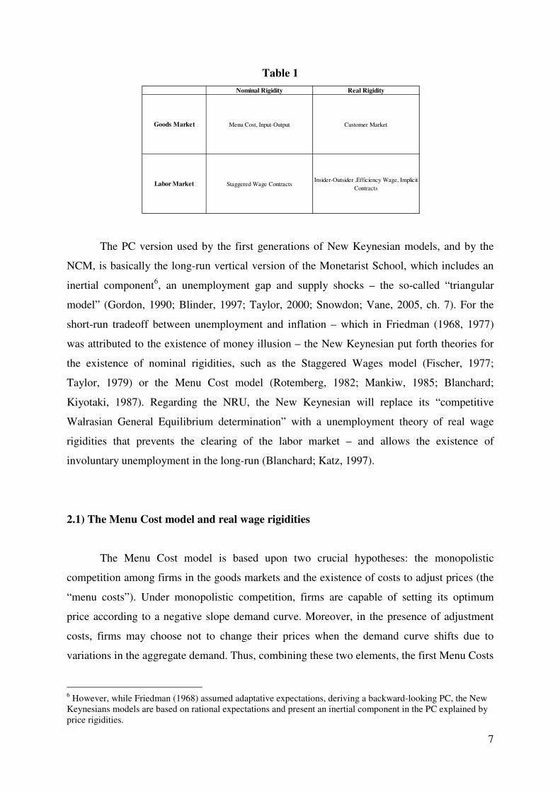
In order to grasp the different kind of rigidities presented in New Keynesian

microfounded models, table 1 represents the different classes of rigidities in terms of a four-

entry matrix: the two rows represent the rigidities in the goods market (price) and labor

market (wages); and the two columns show if there is a nominal or a real rigidity in each

market. The main New Keynesian models for each entry of the matrix are indicated according

to Gordon (Ibid):

2 Lucas (Ibid) accepts that only in the case of surprise, the monetary authority can succeed, in the short-term, in increasing the real output. For a discussion of the differences between the Monetarists and New Classical adjustments of prices and quantities, see Hoover (1984). 3 Of course this critic is part of a broader criticism to the “Keynesian” models made by Lucas (1976). 4 It is worth noting that involuntary unemployment in New Keynesian theory is associated with imperfections in the labor market that prevents its clearing (such as real wage rigidity). This involuntary unemployment definition, hence, is different from the one based on the principle of effective demand. 5 As in the Neoclassical Synthesis, the New Keynesian models assume nominal price or wage rigidity to prevent the Keyne’s and Pigou’s effects in the short-run and, thus, to allow for the non-neutrality of money.

7

Table 1

The PC version used by the first generations of New Keynesian models, and by the

NCM, is basically the long-run vertical version of the Monetarist School, which includes an

inertial component6, an unemployment gap and supply shocks – the so-called “triangular

model” (Gordon, 1990; Blinder, 1997; Taylor, 2000; Snowdon; Vane, 2005, ch. 7). For the

short-run tradeoff between unemployment and inflation – which in Friedman (1968, 1977)

was attributed to the existence of money illusion – the New Keynesian put forth theories for

the existence of nominal rigidities, such as the Staggered Wages model (Fischer, 1977;

Taylor, 1979) or the Menu Cost model (Rotemberg, 1982; Mankiw, 1985; Blanchard;

Kiyotaki, 1987). Regarding the NRU, the New Keynesian will replace its “competitive

Walrasian General Equilibrium determination” with a unemployment theory of real wage

rigidities that prevents the clearing of the labor market – and allows the existence of

involuntary unemployment in the long-run (Blanchard; Katz, 1997).

2.1) The Menu Cost model and real wage rigidities

The Menu Cost model is based upon two crucial hypotheses: the monopolistic

competition among firms in the goods markets and the existence of costs to adjust prices (the

“menu costs”). Under monopolistic competition, firms are capable of setting its optimum

price according to a negative slope demand curve. Moreover, in the presence of adjustment

costs, firms may choose not to change their prices when the demand curve shifts due to

variations in the aggregate demand. Thus, combining these two elements, the first Menu Costs

6 However, while Friedman (1968) assumed adaptative expectations, deriving a backward-looking PC, the New Keynesians models are based on rational expectations and present an inertial component in the PC explained by price rigidities.

Nominal Rigidity Real Rigidity

Goods Market Menu Cost, Input-Output Customer Market

Labor Market Staggered Wage ContractsInsider-Outsider ,Efficiency Wage, Implicit

Contracts

8

models were developed in the eighties (Rotemberg, 1982; Mankiw, 1985; Blanchard;

Kiyotaki, 1987) seeking to generate, in the short-run, price rigidity and the non-neutrality of

money.

Nevertheless, as it’s shown by Romer (1993, 2005), menu costs alone cannot be high

enough in order to compensate the firm’s profit loss of not adjusting prices. That occurs

because whenever the aggregate demand moves, causing a shift of the demand curve, the

firm’s costs – such as wages – also change increasing the firm’s profit losses of not adjusting

prices. Consequently, it is necessary, in order to generate price rigidity, that a real wage

rigidity be added to the Menu Cost model (Blanchard; Kiyotaki, 1987; Ball; Romer, 1990).

Thus, the firm’s costs also become rigid against changes in aggregate demand because real

wage rigidity, when combined with price rigidity, makes the nominal wage also rigid7. In

addition, the adoption of real wage rigidity, through New Keynesian unemployment theory8,

also helps to explain the persistence of involuntary unemployment in the long-run, once the

labor market fails to clear – giving a different meaning to the NRU (Carlin; Soskice, 1990, ch.

6; Blanchard; Katz, 1997).

In the simplified version of the Menu Cost model presented here, it is assumed that

labor is both homogeneous and the only factor of production. In addition, the marginal

productivity of labor is considered constant in order to simplify the analysis of the firm’s

marginal cost. So, according to the model, the economy is formed by N different sectors,

being each one of them monopolized by a single and homogeneous firm9. Additionally,

following Rotemberg (1982), each firm maximizes its objective function taking the price set

by the others as given, which turn the model into a partial equilibrium analysis. Equation (1)

summarizes the maximization problem faced by each one of the N firms:

�á� � = ��� ���

� ; �� − �� �() (1)

The first component on the right hand of the equation is the real revenue of the firm,

which is determined by its relative price ��� and from the quantity sold in the market . This

quantity, in turn, is negatively affected by the relative price and positively affected by the

aggregate demand �. The firm’s real costs are defined by the real wage �� and the quantity

7 It is worth noting that nominal wage rigidity is basically the same mechanism used by the Neoclassical Synthesis to demonstrate the non-neutrality of money in the short-term (Modigliani, 1944). 8 For a discussion of the New Keynesian unemployment theories, see Gordon (1990) and Romer (2005, ch. 9). 9 For a broader variety of imperfect competition, see Carlin and Soskice (2006, ch. 15)

9

of labor � employed in order to produce . Because the general price level is taken as given

by each firm, it can be equal to unity in (1). Therefore, the first order condition for this

problem is:

�∗ = � �

���� ���� (2)

Where �∗ is the optimum price set by each firm, � is the price-elasticity of demand

and MPL is the marginal productivity of labor. It’s worth noting that the price set by each

firms equals a mark-up over the labor unity cost, and the mark-up is a decreasing function of

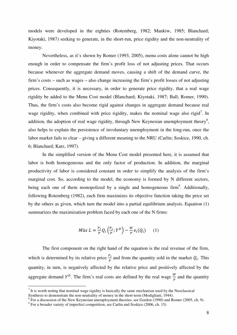
price-elasticity of demand. Figure 1 represents, now, what happens to each firm if the

aggregate demand decreases in terms of a partial equilibrium analysis under monopolistic

competition:

Figure 1

In Figure 1, MC and MR stands for, respectively, the marginal cost curve and the

marginal revenue curve. The marginal cost curve is flat because of our assumption that the

marginal productivity of labor is constant. So, a decrease in aggregate demand causes a shift

to the left of individual demand curve of each firm and its marginal revenue curve.

Conversely, the fall in aggregate demand, in terms of the labor market, provokes a reduction

in labor demand, decreasing real wages – which means that real wages are pro-cyclical in the

short-run –, and moves down the marginal cost curve. Therefore, the initial equilibrium point

to the firm shifts from A to C. Nevertheless, if there are price adjustment costs, the firm may

choose not to change its price and accepts a profit loss. In this case, the firm has to compare

the adjustment cost with the profit loss, which in Figure 1 corresponds to the areas I and II. As

it can be seen both in equation (2) and in Figure 1, the profit loss area is determined by the

price-elasticity of demand and by the change in wages. Romer (2005) points out that, under

10

several assumptions for the parameters determining the areas I and II, an extremely high

adjustment cost would be necessary to compensate the profit loss – given the fall in real

wages.

As a result, the Menu Cost model shows that it is necessary to combine real wage

rigidity with adjustment costs in order to generate price rigidity in the goods market. The need

for real wage rigidity was met by the unemployment theories developed by the New

Keynesian School in the eighties that pointed to the existence of imperfections in the labor

market. At the same time that these theories provided a theoretical argument for real wage

rigidity, they also explained the persistence of involuntary unemployment in the long-run.

Assuming now that real wages do not necessarily decrease when the aggregate

demand is reduced, or that they do not decrease as if there were no imperfections in the labor

market10, the marginal curve in Figure 1 does not move down. In this case, the profit loss of

not adjusting price only corresponds to the area I. If the adjustment cost is higher than this

new profit loss, the firm will have incentives to keep its price fixed for a given decrease in the

aggregate demand. Romer (Ibid) then shows that under these new circumstances a small menu

cost can be higher than the profit loss, and thus the model generates microfoundations of the

firm’s price rigidity.

2.2) The Menu Cost model and the PC

So far, the Menu Cost model has explained the existence of price rigidity that allows

the aggregate demand to affect the real output in the short-run. Additionally, the real wage

rigidity plays a crucial role in order to justify the existence of involuntary unemployment in

the long-run. Nevertheless, the passage from the partial equilibrium analysis to the general

equilibrium is not simple in the Menu Cost model. As it has been said, the model assumes that

firms maximize their objective functions for a given set of prices; otherwise they would not

face a stable individual demand curve and it would be impossible to determine the area

corresponding to the profit loss. Therefore, to move on to the PC derived from this model, it is

assumed that the aggregate supply of this economy is given by the average mark-up of the

firms 1 + � over the labor unit cost:

10 This could be explained, for example, by the efficiency wage theory, or the insider-outsider model (Romer, 2005, ch. 9)

11

� = (1 + � ) �!���!

(3)

Solving (3) for the real wage, the real wage paid by the firms is obtained:

�!�!

= ���(�"#!) (4)

Equation (4) is the price-setting curve that is similar to the labor demand curve in the

New Keynesian labor market. Carlin and Soskice (1990) points out that in the long-run, when

prices are flexible, the mark-up is anti-cyclical, because it is a negative function of the price-

elasticity of the individual demand curves. Nonetheless, they assume a decreasing marginal

productivity of labor, which, in the end, offsets the positive effect of reducing mark-ups over

the real wage. Hence, in the simplified version of the model, it is assumed a flat price-setting

curve. Equation (4) also shows that the real wage is given by an exogenous mark-up and by

labor productivity.

As previously noted, the New Keynesian model assumes that there are imperfections

in the labor market. These imperfections are associated with a wage curve, which replaces the

traditional labor supply curve of New Classical models (Lucas, 1975). These imperfections

may be associated to the fact that labor productivity is a function of real wages or to a strong

market power (or bargain power) of labor unions. Therefore, the wage curve is both flatter

and above the traditional labor supply curve, that is, there is wage rigidity and the real wage

equilibrium does not ensure the full employment of labor. Equation (5) shows the wage curve:

�!�!

= −$% + & (5)

In (5), % is the unemployment rate, $ is a positive parameter and & represents

institutional aspects that may affect the wage negotiation. Solving (4) and (5) for the

unemployment rate:

%' = () − ���!

)(�"#!) (6)

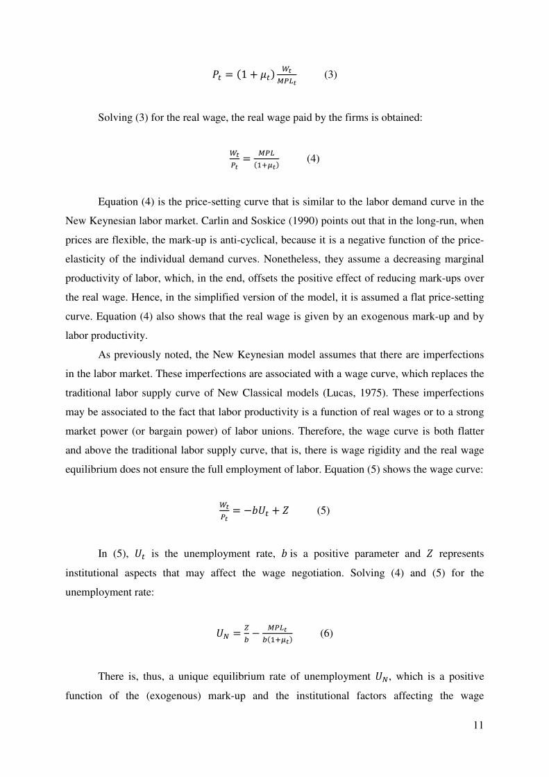
There is, thus, a unique equilibrium rate of unemployment %', which is a positive

function of the (exogenous) mark-up and the institutional factors affecting the wage

12

Source: Own elaboration

A

B

negotiation11. The New Keynesian equilibrium rate of unemployment is different from the

NRU presented by Friedman (1968), once it is explained by imperfections in the labor market

and allows the existence of involuntary unemployment (Carlin; Soskice, 1990, ch. 6;

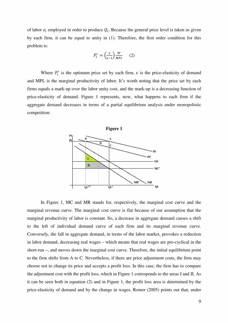
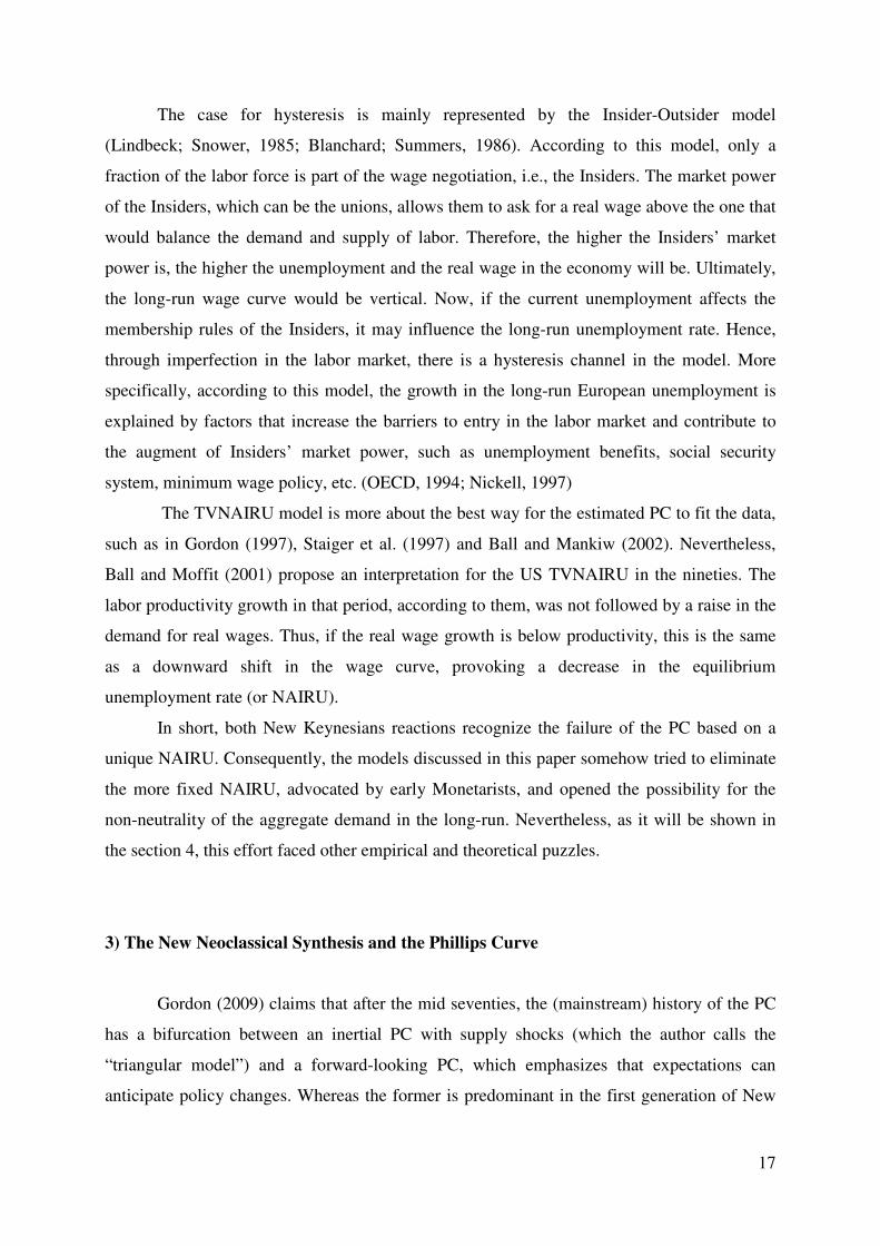
Blanchard; Katz, 1997). Figure 2 presents the New Keynesian labor market described by

equations (4) to (6):

Figure 2

�!�!

���!

(�"*!)

���!

(�"*!+,)

%' %′ %

From the initial equilibrium, given by point A, a negative shock of the aggregate

demand will affect the unemployment rate in the short-run, once firms in the Menu Cost

model have incentives to keep prices fixed reducing the real output of the economy. So, the

actual unemployment rate is %′. This is equivalent to a movement along a short-term PC –

where there is a tradeoff between unemployment and wage12 – and implies a mark-up

increase. It is important to mention that when prices are rigid and the productivity is given,

the actual mark-up is anti-cyclical and the real wages are pro-cyclical (corresponding to shifts

11 This result is in line with the New Keynesian defense of the main determinants of the unemployment rate in the long-run, such as union density, labor protection, unemployment benefits, etc. (Nickell, 1997; OECD, 1994). For a critique of these studies, see Stockhammer and Klar (2011) 12 It is worth noting that in this simple version of the model, real wage and price were considered fixed. The movement along involves price variation; this could be done if we consider that real wages are not fixed, but have only a weak response to aggregate demand changes

PS

WC

PS’

13

along the wage curve and a downward shift from the price-setting curve)13. Nevertheless, the

PC presented by the New Keynesians of the NCM is vertical in the long-run (Blinder, 1997;

Taylor, 2000), which means that the firms will eventually adjust prices and the economy will

move back to its “natural” equilibrium. The dynamic of price adjustment, however, is not

clear in the Menu Cost model. There is no explanation why firms will eventually start to

adjust price. Hence, the lack of an explanation of the PC inertial component, together with the

passage from partial to general equilibrium, poses some difficulties to a formal derivation of

the PC from the Menu Cost micro model: “Unfortunately the menu-cost model does not

translate into a Phillips curve (Carlin; Soskice, 2006, p. 634)”. Ball and Mankiw (1994) claim

that the Menu Cost model should be seen as a parable which captures the basic fact that firms

have the incentives not to adjust price in the short-run.

So, according to this parable, when the economy is in point B, from Figure 2, firms

will eventually (in the long-run) start to have incentives to reduce their prices, bringing back

the economy to the NRU through the Keyne’s and Pigou’s effect or by a response, in terms of

interest rates, of the monetary policy rule. Furthermore, the price adjustment initially slowed

(or blocked) by the existence of menu costs will be complete in the next period. In other

words, there is full inflation inertia in the NCM PC, which in Figure 2 will correspond to a

rapid shift upwards of the price-setting curve14. So, if a positive unemployment gap persists

over time through a recessive monetary or fiscal policy, the economy will face an accelerated

deflation in the long-run. Equation (6) shows the NCM PC with its full inertia component:

. = . �� − /(% − %') + 0 (6)

In (6), . stands for the current inflation, 0 represents supply shocks and / is a

parameter. Because in the NCM the supply shocks are random and zero on average over a

longer period, 0 equals zero in the long-run (Serrano, 2007). Equation (6) can be solved in

terms of the inflation rate resulting in:

∆. = −/(% − %') (7)

13 This is a very important result for the New Keynesian tradition, since the (old) empirical evidence of pro-cyclical real wages (Dunlop, 1938) challenged the literature that maintained Keynes’s first postulate, that is, the labor demand curve. 14 Since Carlin and Soskice (1990) assumes a flat price-setting curve, the long-run real wage is acyclical. In this case, the mark-up, under flexible prices, is anti-cyclical because it is assumed decreasing labor productivity.

14

As equation (7) shows, the NRU is the Non-Accelerating Rate of Unemployment

(NAIRU), the only equilibrium rate of unemployment compatible with stable inflation in the

long-run. This strong result depends on two factors. First, the fact that the mark-up is

exogenous to the real wage bargain in the labor market and, moreover, its variations are offset

by changes in labor productivity (which is the same of a given mark-up combined with fixed

labor productivity). For a given wage curve, this assumption is crucially for the determination

of a unique equilibrium rate of unemployment as it can be seen in Figure 2. Second, the full

inflation inertia assumption is responsible for making a positive unemployment gap in the

long-run a potential source of hyperinflation. Again, it should be observed that, the full inertia

component is not successfully derived from the Menu Cost model.

In summary, the first New Keynesians try to reconcile mainstream macroeconomics

after Monetarism and New Classicism with the “Keynesian” results of the Neoclassical

Synthesis, combining real wage rigidity with price rigidity. The simplified model stressed that

the combination of Menu Cost model and real wage rigidity generates price and nominal

wage rigidity. This result is crucial to restore, in the short-run, the non-neutrality of money,

even in the presence of rational expectations. Furthermore, it was also highlighted that

assuming full inertia in inflation and considering that the mark-up is exogenous to the real

wage bargain in the labor market, the vertical PC based on a single NAIRU is obtained.

Hence, the model combines short-run non-neutrality with long-run neutrality of money.

Indeed, according to the PC presented in the NCM, the persistence of an increase in aggregate

demand, which causes a negative unemployment gap over a longer period of time, will only

bring an accelerated inflation in the long-run.

Nevertheless, it was indicated that the Menu Cost model, associated to real wage

rigidity, was unable to generate the proper microfoundations to price adjustment in the long-

run. Moreover, as it will be shown in the next section, the New Keynesian model based on a

unique NAIRU was subject to empirical criticism because it failed to explain the low inflation

both in Europe and in the USA.

2.3) Some Puzzling Evidences to the NAIRU and its Reactions

Despite its wide adoption in simplified versions of the NCM, the New Keynesians do

not hold a unified view on the strictly vertical PC based upon a unique NAIRU. The empirical

evidence raised by the macroeconomic literature during the eighties and nineties show that the

15

Source: IMF World Economic Outlook

NAIRU model failed to explain the observed relationship between unemployment in some

European countries and in the US (Blanchard; Summers, 1986; Gordon, 1997; Stirati, 2001).

The reactions inside the New Keynesian literature varied from the adoption of the hysteresis

model (Lindbeck; Snower, 1985; Blanchard; Summers, 1986) to a modified version of the

NAIRU, the so-called Time-Varying NAIRU (TVNAIRU) (Gordon, 1997). In both cases, the

New Keynesians had to face the empirical evidence rejecting the validity of the main

argument in favor of the long-run neutrality of money, that is, the existence of a single

NAIRU over time.

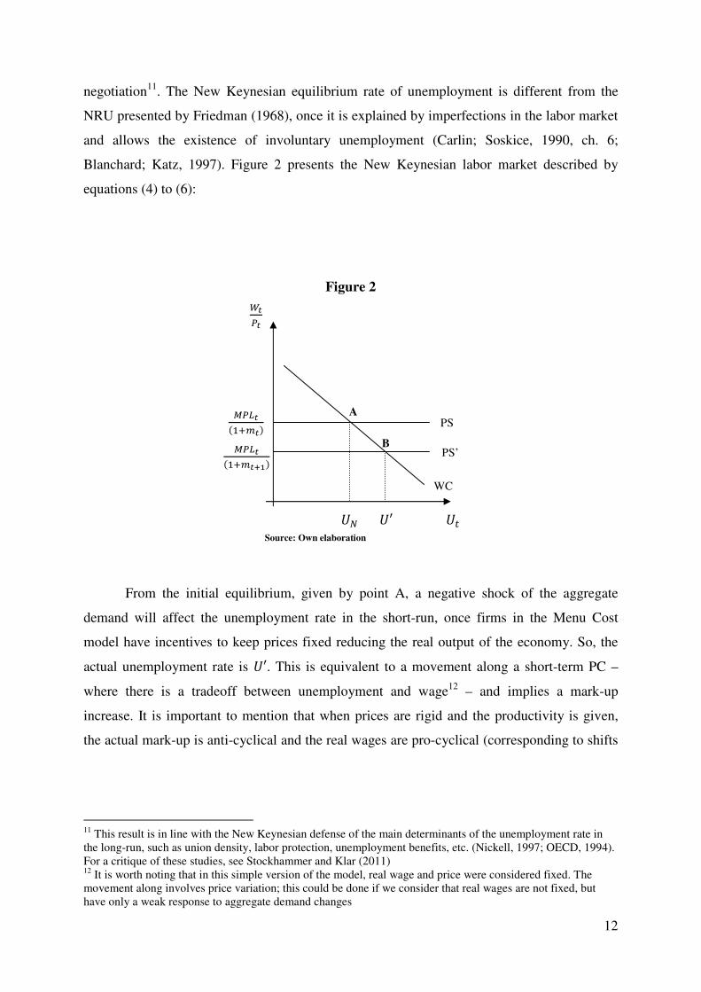
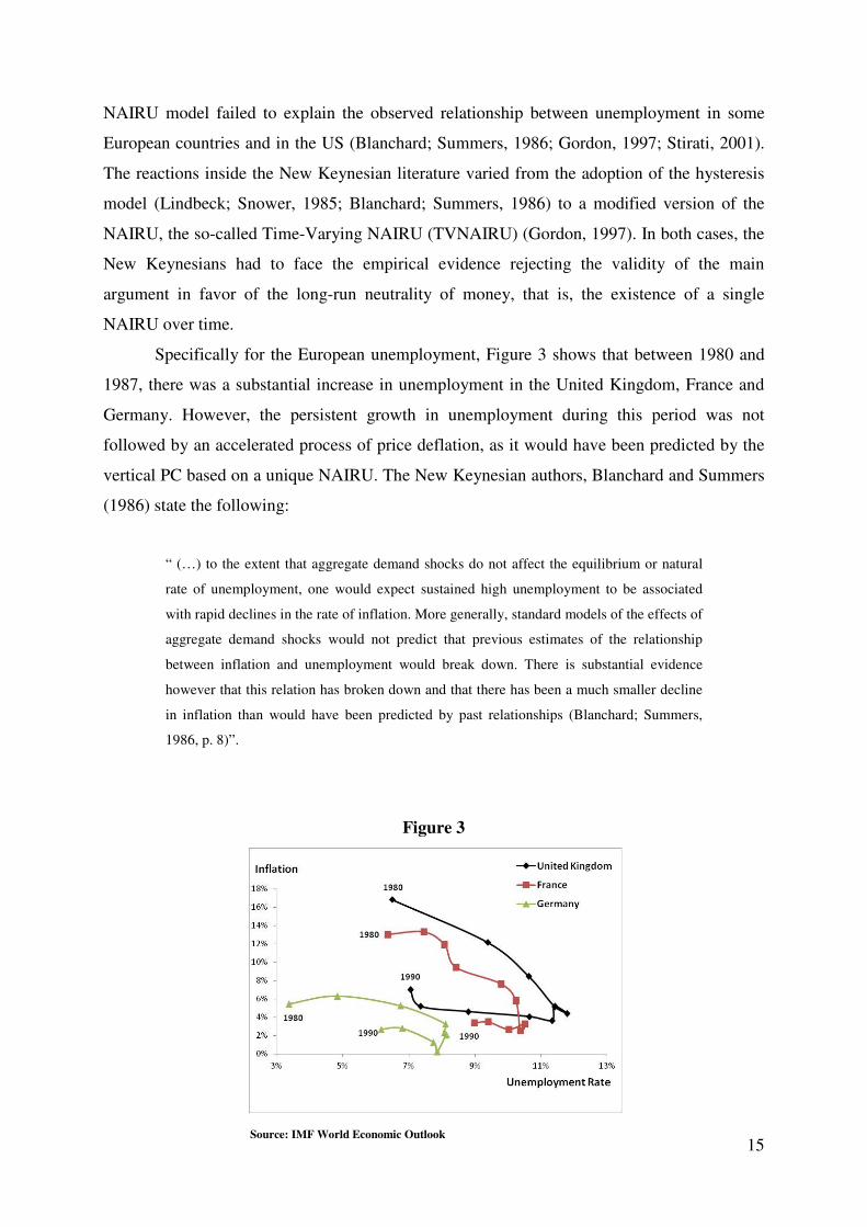
Specifically for the European unemployment, Figure 3 shows that between 1980 and

1987, there was a substantial increase in unemployment in the United Kingdom, France and

Germany. However, the persistent growth in unemployment during this period was not

followed by an accelerated process of price deflation, as it would have been predicted by the

vertical PC based on a unique NAIRU. The New Keynesian authors, Blanchard and Summers

(1986) state the following:

“ (…) to the extent that aggregate demand shocks do not affect the equilibrium or natural

rate of unemployment, one would expect sustained high unemployment to be associated

with rapid declines in the rate of inflation. More generally, standard models of the effects of

aggregate demand shocks would not predict that previous estimates of the relationship

between inflation and unemployment would break down. There is substantial evidence

however that this relation has broken down and that there has been a much smaller decline

in inflation than would have been predicted by past relationships (Blanchard; Summers,

1986, p. 8)”.

Figure 3

16

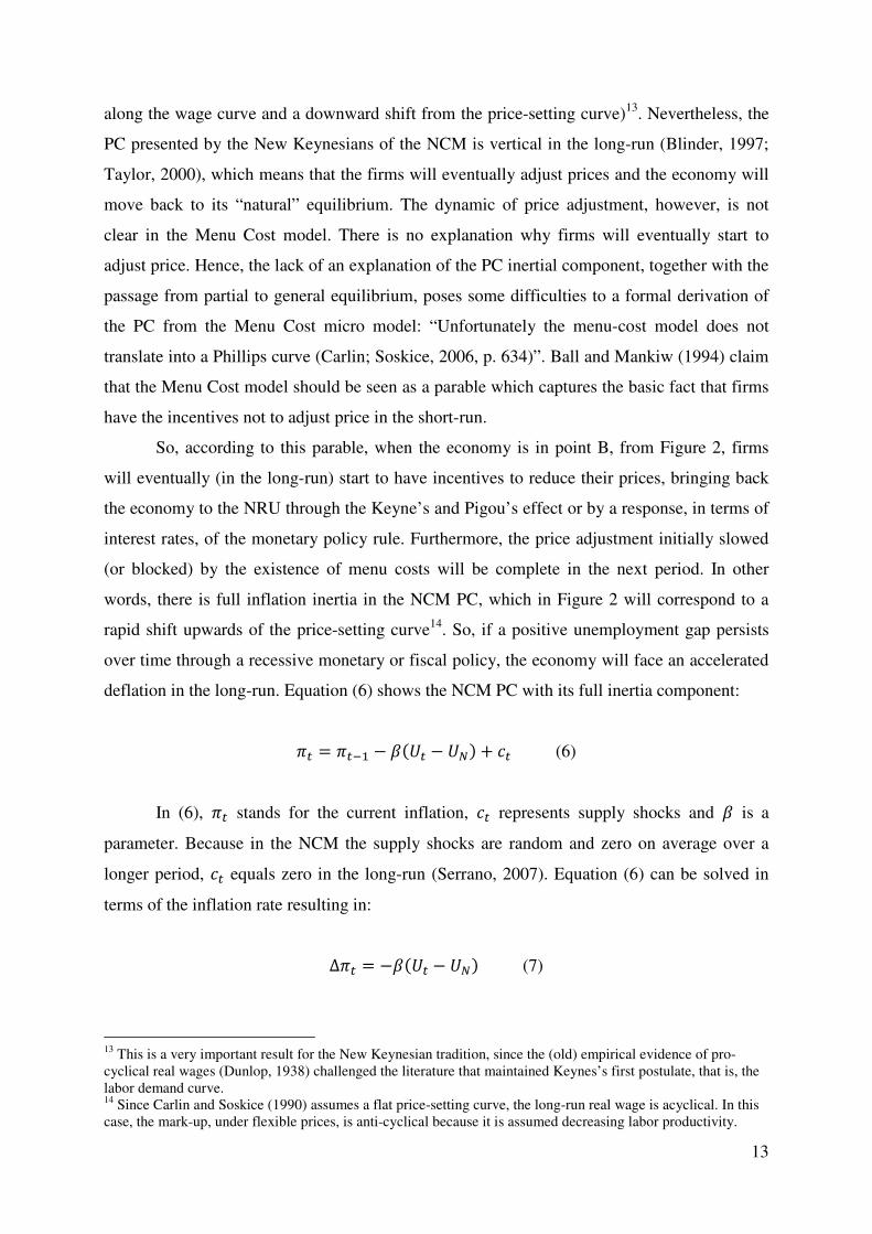
Source: IMF World Economic Outlook

Even the initial fall in prices, observed in the three countries, is strongly influenced by

the fall in the terms of trade of OECD countries during the eighties (Stirati, 2001). Therefore,

according to Figure 3, it seems that the PCs are moving and changing the terms of the tradeoff

between unemployment and inflation, without describing a vertical long-run PC.

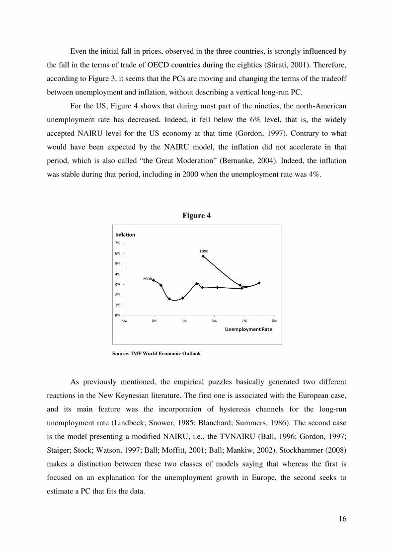
For the US, Figure 4 shows that during most part of the nineties, the north-American

unemployment rate has decreased. Indeed, it fell below the 6% level, that is, the widely

accepted NAIRU level for the US economy at that time (Gordon, 1997). Contrary to what

would have been expected by the NAIRU model, the inflation did not accelerate in that

period, which is also called “the Great Moderation” (Bernanke, 2004). Indeed, the inflation

was stable during that period, including in 2000 when the unemployment rate was 4%.

Figure 4

As previously mentioned, the empirical puzzles basically generated two different

reactions in the New Keynesian literature. The first one is associated with the European case,

and its main feature was the incorporation of hysteresis channels for the long-run

unemployment rate (Lindbeck; Snower, 1985; Blanchard; Summers, 1986). The second case

is the model presenting a modified NAIRU, i.e., the TVNAIRU (Ball, 1996; Gordon, 1997;

Staiger; Stock; Watson, 1997; Ball; Moffitt, 2001; Ball; Mankiw, 2002). Stockhammer (2008)

makes a distinction between these two classes of models saying that whereas the first is

focused on an explanation for the unemployment growth in Europe, the second seeks to

estimate a PC that fits the data.

17

The case for hysteresis is mainly represented by the Insider-Outsider model

(Lindbeck; Snower, 1985; Blanchard; Summers, 1986). According to this model, only a

fraction of the labor force is part of the wage negotiation, i.e., the Insiders. The market power

of the Insiders, which can be the unions, allows them to ask for a real wage above the one that

would balance the demand and supply of labor. Therefore, the higher the Insiders’ market

power is, the higher the unemployment and the real wage in the economy will be. Ultimately,

the long-run wage curve would be vertical. Now, if the current unemployment affects the

membership rules of the Insiders, it may influence the long-run unemployment rate. Hence,

through imperfection in the labor market, there is a hysteresis channel in the model. More

specifically, according to this model, the growth in the long-run European unemployment is

explained by factors that increase the barriers to entry in the labor market and contribute to

the augment of Insiders’ market power, such as unemployment benefits, social security

system, minimum wage policy, etc. (OECD, 1994; Nickell, 1997)

The TVNAIRU model is more about the best way for the estimated PC to fit the data,

such as in Gordon (1997), Staiger et al. (1997) and Ball and Mankiw (2002). Nevertheless,

Ball and Moffit (2001) propose an interpretation for the US TVNAIRU in the nineties. The

labor productivity growth in that period, according to them, was not followed by a raise in the

demand for real wages. Thus, if the real wage growth is below productivity, this is the same

as a downward shift in the wage curve, provoking a decrease in the equilibrium

unemployment rate (or NAIRU).

In short, both New Keynesians reactions recognize the failure of the PC based on a

unique NAIRU. Consequently, the models discussed in this paper somehow tried to eliminate

the more fixed NAIRU, advocated by early Monetarists, and opened the possibility for the

non-neutrality of the aggregate demand in the long-run. Nevertheless, as it will be shown in

the section 4, this effort faced other empirical and theoretical puzzles.

3) The New Neoclassical Synthesis and the Phillips Curve

Gordon (2009) claims that after the mid seventies, the (mainstream) history of the PC

has a bifurcation between an inertial PC with supply shocks (which the author calls the

“triangular model”) and a forward-looking PC, which emphasizes that expectations can

anticipate policy changes. Whereas the former is predominant in the first generation of New

18

Keynesian models – especially in the NCM –, the latter is the basis for the New Keynesian

Phillips Curve (NKPC) presented in the New Neoclassical Synthesis (NNS) models15.

The NNS model is actually very similar to the NCM. Both of them are basically

defined by the “3-equation model” (Carlin; Soskice, 2006, ch. 3), namely: an IS equation, a

PC and a monetary rule. However, their main differences are the theory behind these

equations and the specification of the PC. The NSN models combine the RBC modelling, i.e.,

the Dynamic Stochastic General Equilibrium (DSGE) model, with New Keynesian frictions,

such as price or wage rigidity. For this reason, the PC derived from this model has a different

specification that stresses the forward-looking expectations and a dynamic rule for price

setting.

The adoption of the RBC modelling implies a different approach to the business cycle.

In particular, the NNS basic models abandoned the New Keynesian idea of non-market

clearing. The seminal works from by RBC School are Kydland and Prescott (1982) and

Nelson and Plosser (1982). The latter estimated 14 economic series for the US to test the

existence of a unit root in each series. In particular, they confirmed the existence of a unit root

in the GDP and employment series, which implies that such series have a stochastic trend and

are not mean reversing. In other words, it is not possible to isolate the determinants of the

GDP cycle from the ones of the GDP trends. This is a problematic result for the New

Keynesianism since its models postulate the division between the cycle components (the

aggregate demand) and the trend components (aggregate supply). Therefore, the RBC answer

is to claim that both cycle and trend are determined by supply factors. The traditional RBC

model (Kydland; Prescott, 1982) presents a market clearing interpretation of the business

cycle. There is no room in this model for market disequilibrium, such as involuntary

unemployment, even in the short-run.

The cycles in the RBC tradition are then seen as optimal responses of representative

agents (with rational expectations) to random supply shocks. The inexistence of real rigidities,

such as in the New Keynesianism, allows an automatic market clearing. There is no

involuntary unemployment in NNS models, for the representative agent is always on his labor

supply curve16. On the other hand, the “Keynesian” side of this kind of model appears on the

existence of price rigidities that allow the non-neutrality of money in the short-run and are

combined with nominal wage flexibility. Hence, the cyclical changes in real wages that come

15 See, for example, Goodfriend and King (1997) and Clarida et al. (1999). 16 For an example of a NNS model with real rigidities and involuntary unemployment, see Blanchard et al. (2007)

19

with the pro-cyclical oscillations of aggregate demand and output, due to price rigidities, are

assumed to allow the labor supply to adjust the cyclical labor demand, preventing the changes

in aggregate demand and output from generating any involuntary unemployment. Goodfriend

and King (1997) introduce nominal rigidity through imperfect competition and the price

adjustment dynamics presented by Calvo (1983). His model provides a theoretical foundation

for price rigidity without using real rigidities, such as in the Menu Cost model, which,

conversely, failed to provide the PC inertial component with microfoundations.

It is also worth saying that DSGE models became prevailing in the macroeconomic

mainstream from the mid-nineties on. Woodford (2009) even points out that DSGE modelling

is the starting point to any academic debate in the field of macroeconomics. Consequently, the

DSGE framework and the NNS model are seen as a greater process of convergence in

macroeconomics. According to this view, any divergence in macroeconomics could be

disputed in terms of a DSGE model. Finally, one of the main precursors of the NNS

prescribes a general rule to write articles:

“A macroeconomic article today often follows strict, haiku-like rules. It starts from a

general equilibrium structure, in which individual maximize the expected present value of

utility, firms maximize their value, and markets clear. Then, it introduces a twist, be it an

imperfection or the closing of a particular set of markets, and works out the general

equilibrium implications. It then performs a numerical simulation based on calibration,

showing that the model performs well. It ends with a welfare assessment (Blanchard, 2009,

p. 225)”.

3.1) Calvo’s model and The New Keynesian Phillips Curve

The Calvo’s model is the starting point to derive the NKPC, which allows for the

existence of the tradeoff between wages and unemployment in the short-run (or the non-

neutrality of money). In this model, as well as in the Menu Cost model, there is an assumption

of monopolistic competition in the markets. Consequently, the optimum price set by the firm

is the same as equation (2) shows. Additionally, although firms have rational expectations

about the future, there are exogenous random effects that may prevent them from adjusting

price, and this is crucial to the model. As a result, firms do not have control over when they

will be able to adjust price and only a random fraction of the firms can adjust price in each

period. Thus the NNS model provides an explanation for price rigidity in the context of a

20

general equilibrium analysis without reference to real rigidities, which would prevent the

markets clearing.

A simplified version of this model is presented here in order to derive the NKPC,

based on Woodford (2003), Goodfriend (2004), Carlin and Soskice (2006, ch. 15) and

Wickens (2008). Considering, then, that labor is the only factor of production, its marginal

productivity is constant and the demand curves have constant elasticity, it follows,

consequently, equation (8) – which presents the optimum price set by the firms:

�∗ = � �2

�2��� ���� (8)

The only difference between equations (2) and (8) is the fact that in the latter the

firm’s mark-up is constant precisely because the price-elasticity of demand is constant

(Goodfriend, 2004). Therefore, there is an optimum mark-up desired by each firm.

Furthermore, this mark-up will be the one obtained by the firms when there is no price

rigidity. Rewriting equation (8) in order to stress the optimum (and exogenous) mark-up �∗:

�∗ = (1 + �∗) �

��� (9)

Nevertheless, in the Calvo’s model, only a random portion of the firms can adjust their

price in each period in order to attain the optimum mark-up. In addition, because firms have

forward-looking expectations, they adjust their prices aiming to minimize the distance

between their actual and optimum mark-up. If it is further considered that the general price

level is an average of the sector’s prices, it follows that:

34� = 534�∗ + (1 − 5)34� �� (10)

34� − 34� �� = 534�∗ − 534� �� (11)

. = 5.∗ (12)

In equations (10) to (12) 5 is the random fraction of firms that could adjust its prices

at the moment 6, �∗ is the optimum price when firms obtain their optimal mark-up and .∗ is

the optimal price inflation. If every firm could adjust price in each period, .∗ would be the

economy’s inflation rate. Since only a fraction 5 adjusts its price, the inflation is given by

21

5.∗. .∗, in turn, is a function of inflation expectations and the deviations from the optimum

mark-up. Therefore, this function is given by equation (13)

.∗ = 78"�9 . "� + $(� − �∗) (13)

In equation (31), 9 . "� stands for the expectations about future inflation, �∗ and �

are, respectively, the optimum and the actual mark-up; and 78"� and $ are positive

parameters. Under the Calvo’s model, the current mark-up may deviate from its optimum in

case firms are unable to adjust prices. Additionally, the NNS literature (Rotemberg;

Woodford, 1999) says that the actual mark-up is anti-cyclical, for in RBC models the real

wages are pro-cyclical – since this model presents a positive slope labor supply curve.

Accordingly, if in Calvo’s model prices are rigid, the aggregate demand affects the real output

and the level of employment in the short-run. For a given labor supply curve, firms have to

pay higher real wages in order to increase their production, which, in the case of constant

labor marginal productivity, results in an anti-cyclical mark-up. Therefore, whenever the

aggregate demand expands the economy above the equilibrium given by a flex price RBC

model, the actual mark-up falls below its optimum level. This gap makes the firms increase

their prices whenever possible. That is why the mark-up gap has a positive impact on .∗.

Substituting equation (13) with (12), it follows:

. = 578"�9 . "� + 5$(� − �∗) (14)

Equation (14) corresponds to the NKPC. Instead of an inertial component, this version

presents a forward-looking component, which can make the PC shift, anticipating policy

changes that affects the aggregate demand. Moreover, because the actual mark-up is anti-

cyclical, an excess aggregate demand is translated into a positive mark-up gap. This positive

gap causes an inflation pressure until the current mark-up reaches its optimum level. If

equation (14) is recursively solved, it follows:

. = 5$(� − �∗) + 5$ ∑ 9��(� − �∗);< "� (15)

Equation (15) stresses the fact that forward-looking expectations in this model means

that firms care about future deviations of their mark-up relative to its optimum level. In other

words, the actual inflation equals the sum of the current mark-up gap over the future expected

22

gaps. So, if the firms believe that in the future their mark-up will converge towards their

optimum level, 9 . "� in equation (14) declines, which reduces the inflation pressure of an

expansionary policy. Gordon (2009) highlights that this approach to the PC is influenced by

the tradition of the literature about policy’s credibility in order to control inflation, such as the

works by Kydland and Prescott (1977) and Sargent (1982). Indeed, Woodford (2003) and

Goodfriend and King (1997) emphasize the importance of policy’s credibility in order to

ensure that expected future mark-ups will converge to their the optimum level.

Equation (15) can be modified aiming to allow for the existence of some inertial

inflation. Clarida et al. (1999) propose the hybrid NKPC, which combines a forward-looking

component with an inertial component. The model can accommodate this result if it assumes

that the firms unable to adjust their prices optimally, in a given period, use a rule of a thumb

to fix their prices. In this sense, firms could choose any rule of thumb to adjust their price.

Clarida et al. (1999) assumes that firms choose to index their price to past inflation – however

it is not explained why firms do not choose other rules of thumb. Therefore, equations (15)

can be rewritten as follows:

. = 578"�9 . "� + 78��.8�� + 5$(� − �∗) (16)

The hybrid NKPC presented in (16) combines both the effects of forward-looking

expectations and the inflation inertia. Furthermore, if the sum of 578"� over 78�� equals unity,

a persistent positive mark-up gap will cause not just a rise in inflation, but also its acceleration

– which is very similar to the New Consensus PC with an inertial component (Serrano, 2007).

3.2) The Natural Rate of Unemployment in the NKPC

Besides its forward-looking term, the NKPC distinguishes itself from the New

Consensus PC by the use of the mark-up, an “explicit microfoundation”, as a source of

inflation pressure. Wickens (2008) mentions the empirical troubles which the first New

Keynesians had to face because they used the unemployment gap in the formal representation

of the PC. The author says:

“Later, in the 1990s, the evidence seemed to show that the natural rate of unemployment

varied as much as the actual rate of unemployment, thereby largely destroying any link

23

A

B

Source: Own elaboration

between inflation and unemployment. This led to the development of the New Keynesian

Phillips curve. This is closely related to the NAIRU model, but it has more explicit

microfoundations and does not depend on unemployment to provide the driving variable

linking the real economy to inflation (Wickens, 2008, p. 229)”.

Nevertheless, it is possible to show the existence of a unique long-run equilibrium rate

of unemployment (or a “natural rate of unemployment) behind the given optimum mark-up in

the NKPC. Actually, it can be shown that again the long-run non-neutrality of money is based

on a single equilibrium rate of unemployment.

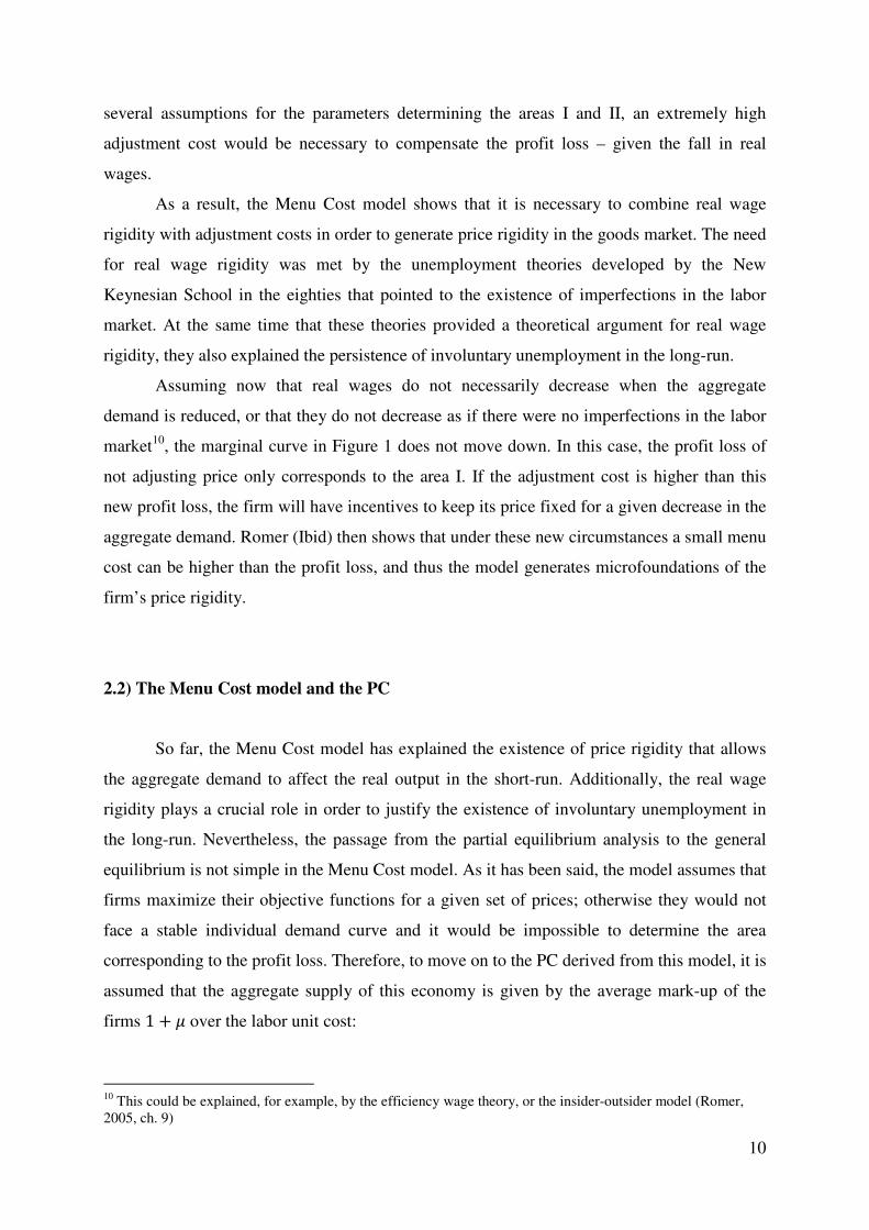
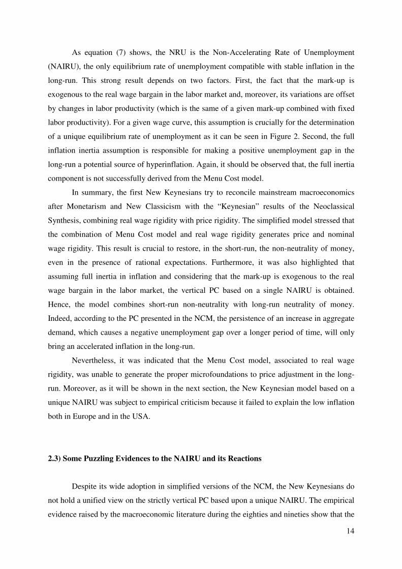
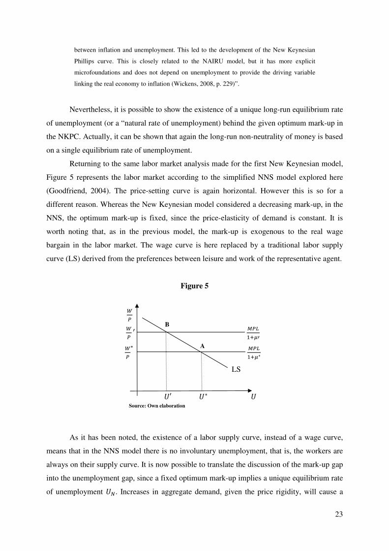
Returning to the same labor market analysis made for the first New Keynesian model,

Figure 5 represents the labor market according to the simplified NNS model explored here

(Goodfriend, 2004). The price-setting curve is again horizontal. However this is so for a

different reason. Whereas the New Keynesian model considered a decreasing mark-up, in the

NNS, the optimum mark-up is fixed, since the price-elasticity of demand is constant. It is

worth noting that, as in the previous model, the mark-up is exogenous to the real wage

bargain in the labor market. The wage curve is here replaced by a traditional labor supply

curve (LS) derived from the preferences between leisure and work of the representative agent.

Figure 5

��

�� ′ ���

�"#=

��

∗

����"#∗

LS

%′ %∗ %

As it has been noted, the existence of a labor supply curve, instead of a wage curve,

means that in the NNS model there is no involuntary unemployment, that is, the workers are

always on their supply curve. It is now possible to translate the discussion of the mark-up gap

into the unemployment gap, since a fixed optimum mark-up implies a unique equilibrium rate

of unemployment %'. Increases in aggregate demand, given the price rigidity, will cause a

24

fall in actual mark-up, which decreases from �∗ to �, because firms have to raise the real

wage in order to employ more workers. The unemployment rate decreases from %∗ to %′. This

lower mark-up, associated to a lower unemployment rate, will generate an inflation pressure

because firms want to increase their mark-ups. Therefore, the mark-up gap can be rewritten in

terms of an unemployment gap. Rewriting the hybrid NKPC with the unemployment gap,

follows equation (17), which is very similar to the New Consensus PC presented in (6).

. = 578"�9 . "� + 78��.8�� + 5$(%∗ − % ) (17)

Despite the innovations brought forward by the NNS model the NKPC is very close to

the New Consensus NAIRU model. If it is assumed that the sum of the parameters associated

with the forward-looking over the inertial component equals unity, the equilibrium

unemployment rate %∗ will have the same effect on the PC that the NAIRU had. Hence, the

single equilibrium unemployment rate is still present and implies the long-run neutrality of

money.

In short, it was argued that one of the factors that contributed to the incorporation of

the RBC modeling in the NNS was the empirical evidence of hysteresis in output and

employment. Therefore, cycles are only driven by supply elements, which implies that

workers are always on the supply labor curve. However, the NNS had also to be compatible

with the New Keynesian feature of short-run non-neutrality of money. In this context, Calvo’s

model was convenient, for it theoretically justified the existence of nominal price rigidity

without assuming real wage rigidity. Moreover, because the model assumes the full

incorporation of expected and inertial inflation, and a single optimal mark-up, it presents a

unique equilibrium rate of unemployment very similar to the NAIRU, implying the long-run

neutrality of money.

4) A Critical Assessment of the NCM’s PC and the NKPC: a summary

4.1) A Critical Assessment of the NAIRU

Section 2 showed some problematic aspects of the NAIRU model. It was emphasized

that the Menu Cost model, combining real wage rigidity and price rigidity, failed to provide

the required theoretical arguments to the inertial component of the PC. More specifically, the

25

model does not explain the price adjustment dynamics, i.e., the reason why and at what

intensity firms adjust their prices in the long-run. Indeed, it is not clear why the adjustment

costs in the course of time cease to be an impeditive to price adjustment. In this context,

Calvo (1983) seems to provide a clearer argument to price adjustment mechanism – which

may help to explain its broader acceptation in mainstream macroeconomics from the mid-

nineties on.

The lack of proper microfoundations to the inertial component in the PC is especially

problematic, since the full inertia assumption, presented in equation (6), is a central aspect of

the NAIRU model. Under full inertia, the unemployment gap causes the acceleration of

inflation and the long-run PC becomes vertical – resulting in the long-run neutrality of

money. The equilibrium unemployment becomes, then, the NAIRU. Nevertheless, full inertia

in the PC, as it has been stressed, is basically an assumption of the NCM, since the Menu Cost

model does not explain why partial inertial (only a part of past inflation being incorporated in

current inflation) is not a possible result of price rigidity in the short-run17.

A second critique that can be raised against the NCM refers to the NAIRU. According

to the discussion in section 2, empirical evidences demonstrated the failure of the PC based

upon a unique NAIRU to explain the behavior of unemployment and inflation both in Europe

and in the US. Indeed, it was not observed in both cases either a period of accelerated

deflation, when the unemployment rate was persistently below its natural level, or of

hyperinflation, when the unemployment rate in the US was below the historical limit of 4%.

The New Keynesian tradition addressed these empirical puzzles to the theory

abandoning the idea of a unique NAIRU, defending either the hysteresis approach or the

TVNAIRU model. The hysteresis argument is particularly problematic because in case the

unemployment rate presents strong hysteresis, the NAIRU loses its relevance in the model

(Gordon, 1989). Equations (18) and (19) illustrate this point:

% ' = >% �� + ? (18)

In the presence of hysteresis, the long-run unemployment rate % ' is explained by the

past unemployment rate plus a white noise ?. Strong hysteresis is defined if > equals unity. In

this case, substituting (18) in (7), the NCM long-run PC, equation (19) is obtained:

17 Gordon (1990) also mentions the Input-Output argument as an explanation for price rigidity and inflation inertia. However, this argument does not justify the adoption of full inertia instead of partial inertia.

26

∆. = −$(% − % ��) + $? (19)

It is not difficult to see that in this case the model, under the assumption of strong

hysteresis, does not exhibit a NAIRU anymore. The acceleration of inflation in (19) is a

function of the variation of the unemployment rate in time.

The only case where a NAIRU independent of time is maintained is when > is below

unity, i.e., in case of weak hysteresis. The evidence of weak hysteresis in the unemployment

rate is precisely the result found initially by Nelson and Plosser (1982) for the US economy,

that is, the absence of an unit root in its series. In this case, according to the New Keynesian

model, the actual unemployment converges to the equilibrium rate of unemployment that is

constant over time. Therefore, although at first the hysteresis and TVNAIRU models seemed

to allow for non-neutrality in the long-run, they are ultimately limited by a long-run constant

unemployment rate.

It is also important to highlight that the fact that the solution of a Time Varying

NAIRU, aiming to adapt the PC to the data, seems an average of the observed unemployment

rate in time. Galbraith (1997) points out that the New Keynesians are in disaccord about the

“true” value of the TVNAIRU. Consequently, if the NAIRU can be anything (in particular

different estimated averages of the unemployment rate series), it may not provide an

appropriate guide to macroeconomic policy.

Finally, the empirical literature initiated by Nelson and Plosser (1982), who tested for

the existence of a unit root in GDP series, proved that the New Keynesian distinction between

the non-neutrality of aggregate demand in the short-run and its neutrality in the long-run has

not been confirmed by the historical data. Although the evidence of weak hysteresis in the

unemployment rate allows for a stable level of the variable in the long-run – which is in

accord with the supply side economics in a longer period –, the stochastic trend found for the

GDP and employment level showed the impossibility of such a distinction (between demand

and supply factor) in these series18. Therefore, trend and cycle, according to the data, should

be explained in the same way, both by aggregate supply or both by aggregate demand

components (Libânio, 2009). In any case, this finding poses a problem to the distinction

between aggregate demand affecting output in the short-run and the supply side economics in

the long-run.

18 For a more recent discussion of this subject, as well as the New Keynesian reactions to Nelson and Plosser (1982), see Libânio (2009).

27

4.2) A Critical Assessment of the NKPC

The NNS seems to have solved two of the biggest problems of the first generations of

New Keynesian models. Firstly by introducing a RBC model, it gave an answer to the fact

that the economy has to be explained by the same factors both in the short and in the long-run.

Secondly, presenting an equilibrium theory of business cycle (without any real rigidity) and

introducing forward-looking expectations, the NNS tried to develop an alternative to the

NAIRU model – which has shown many empirical and theoretical problems.

However the NKPC is also subject to criticism. First, some authors in the New

Keynesian literature, who apparently are not included in the NNS, criticize the forward-

looking component both in the traditional NKPC and in the hybrid version. Eller and Gordon

(2003) and Fuhrer (1997) present empirical tests refuting the statistical significance of the

forward-looking component. According to these estimations, the PC with an inertial

component fits the data for the US economy better. Gordon (2009) also highlights the

implausibility of the forward-looking component. As shown in equation (15), the current

inflation could be totally explained by the sum of the actual over expected future deviations of

the mark-up (or the unemployment rate) in relation to its optimum level. Inflation, in this

case, is not correlated with supply shocks or with inflation inertia.

The second critique deals with the RBC modeling, more specifically, the RBC as an

equilibrium theory of business cycle. According to this model, there is no involuntary

unemployment in the economy, i.e., all the current unemployment is frictional or voluntary. In

this case, recessions are characterized by periods when workers are reluctant to accept the

current real wage and choose not to work. If this were true, the existent unemployment data

would have to be discarded, given that the high unemployment rate currently observed both in

Europe and in the US would be based on people looking for jobs at real wages higher than the

current real wage rather than at the current real wage. The unemployed are, thus, either lying

to the statistics office workers or misunderstand what it means to be “looking for work” in the

recent period. In brief, in the traditional NNS model, the actual high unemployment rates in

advanced countries have to be explained either by an increase in the equilibrium rate of

unemployment (caused by a change in productivity or workers’ preferences) or by the

misleading labor statistics – which does not seems to be the case19.

19 It could be mentioned a third critique made by Pivetti (2008), who criticizes the relationship between mark-up and nominal interest rate derived from the NNS model. According to the NNS model, if the monetary authority

28

5) Final Remarks

Through a simplified model, this article explored the recent evolution of the

neoclassical interpretation of the PC. It tried to show how this interpretation evolved from the

traditional Neoclassical Synthesis approach, in which there is a permanent tradeoff between

inflation and unemployment, into a vertical long-run PC centered on a unique equilibrium rate

of unemployment. More specifically, both the NCM and the NNS models helped to shift the

Neoclassical Synthesis approach, in which excess demand causes “demand-pull” inflation, to

a different approach, in which excess demand causes an acceleration of inflation (Serrano,

2007).

It was argued that the evolution of the New Keynesian microfoundations of the PC

consisted of an effort to react to the theoretical and empirical puzzles faced by the aggregate

models in order to generate both the short-run non-neutrality and long-run neutrality of

money. In particular, the article addressed the evolution from the first NAIRU model to the

NNS model through the analysis of the labor market and of price and wage rigidities in each

of the two models. Whereas the NAIRU model is based on the combination of the Menu Cost

model with real wage rigidity to justify the short-run non-neutrality, the NNS model uses the

Calvo’s model without real wage rigidity.

Regarding the long-run neutrality of money, the paper tried to demonstrate, in section

2, that the unique NAIRU is derived from two assumptions: the full incorporation of past

inflation and an decreasing exogenous mark-up combined with a decreasing marginal

productivity of labor. Additionally, section 3 showed that a unique equilibrium rate of

unemployment that does not accelerate inflation, very similar to the NAIRU, is also found in

the model. Basically, its existence depends on the assumption of a given unique optimum

mark-up and full incorporation of expected future inflation (and past inflation in the case of

the hybrid NKPC).

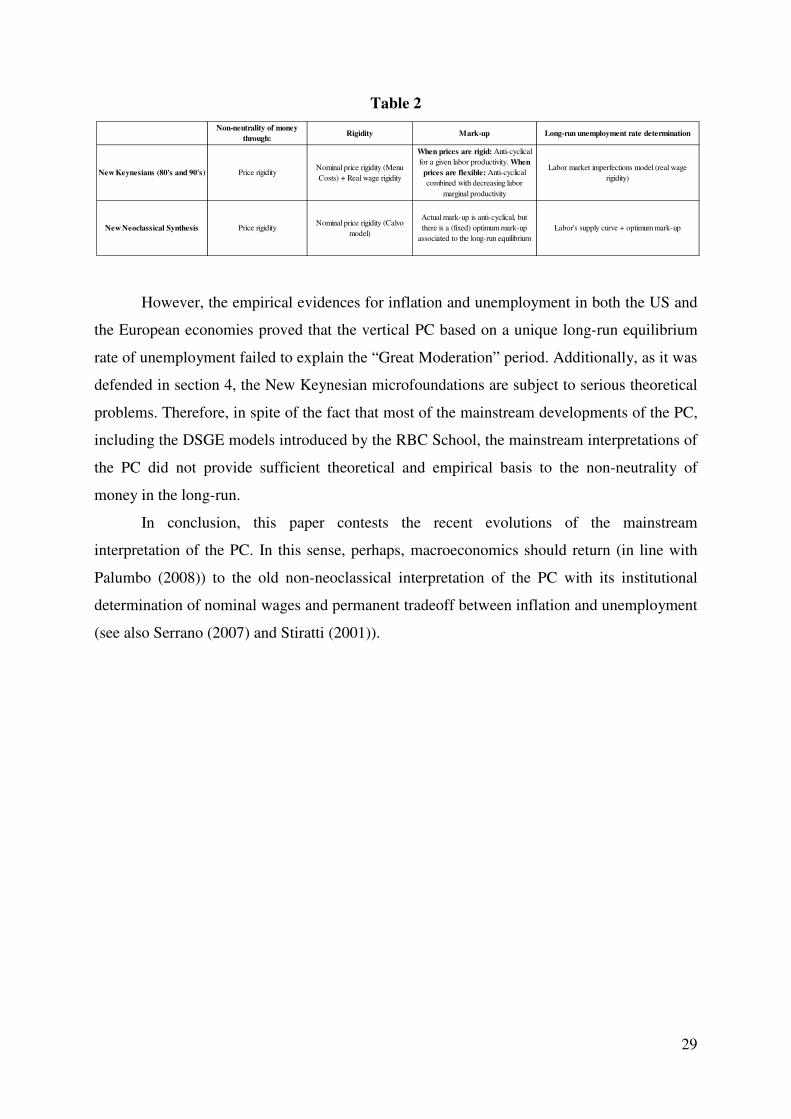
Table 2 below summarizes the basic elements from both the first New Keynesian

models and the NNS that characterizes an economy with a short-run tradeoff between

inflation and unemployment, but with a neutrality of money in the long-run.

increases the nominal interest rate, the aggregate demand and, thus, the output (and employment) will be reduced in the short-run. Consequently, real wages will also fall down and, given the price rigidity, the actual mark-ups will increase. Hence, there is a positive correlation, in the short-run, between nominal interest rate and mark-ups. However, as the economy has an optimum mark-up, Pivetti (Ibid) stresses that when firms become able to adjust price, they will reduce their prices (and their actual mark-up) in order to obtain the optimum mark-up, which is not influenced by the increase in the nominal interest rate. In brief, Pivetti (Ibid) criticizes the distributional neutrality of monetary policy in the NNS model.

29

Table 2

However, the empirical evidences for inflation and unemployment in both the US and

the European economies proved that the vertical PC based on a unique long-run equilibrium

rate of unemployment failed to explain the “Great Moderation” period. Additionally, as it was

defended in section 4, the New Keynesian microfoundations are subject to serious theoretical

problems. Therefore, in spite of the fact that most of the mainstream developments of the PC,

including the DSGE models introduced by the RBC School, the mainstream interpretations of

the PC did not provide sufficient theoretical and empirical basis to the non-neutrality of

money in the long-run.

In conclusion, this paper contests the recent evolutions of the mainstream

interpretation of the PC. In this sense, perhaps, macroeconomics should return (in line with

Palumbo (2008)) to the old non-neoclassical interpretation of the PC with its institutional

determination of nominal wages and permanent tradeoff between inflation and unemployment

(see also Serrano (2007) and Stiratti (2001)).

Non-neutrality of money

through:Rigidity Mark-up Long-run unemployment rate determination

New Keynesians (80's and 90's) Price rigidityNominal price rigidity (Menu Costs) + Real wage rigidity

When prices are rigid: Anti-cyclical for a given labor productivity. When

prices are flexible: Anti-cyclical combined with decreasing labor

marginal productivity

Labor market imperfections model (real wage rigidity)

New Neoclassical Synthesis Price rigidityNominal price rigidity (Calvo

model)

Actual mark-up is anti-cyclical, but there is a (fixed) optimum mark-up

associated to the long-run equilibriumLabor's supply curve + optimum mark-up

30

REFERENCES:

BALL, L. Disinflation and the Nairu: NBER Working Paper. [S.l.] National Bureau of Economic Research Cambridge, Mass., USA, 1996.

BALL, L.; MANKIW, N. G. A Sticky-Price Manifesto: NBER Working Paper. [S.l.] National Bureau of Economic Research Cambridge, Mass., USA, 1994.

BALL, L.; MANKIW, N. G. The NAIRU in Theory and Practice: NBER Working Paper. [S.l.] National Bureau of Economic Research Cambridge, Mass., USA, 2002.

BALL, L.; MOFFITT, R. A. Productivity Growth and the Phillips Curve: NBER Working Paper. [S.l.] National Bureau of Economic Research Cambridge, Mass., USA, 2001.

BALL, L.; ROMER, D. Real Rigidities and the Non-neutrality of Money. Review of

Economic Studies, v. 57, n. 2, p. 183–203, 1990.

BERNANKE, B. S. The Great Moderation: Remarks by Governor Ben S. Bernanke at the meetings of the Eastern Economic Association, Washington, DC February 20, 2004. Eastern

Economic Association, Washington, DC, v. 20, 2004.

BLANCHARD, O. The State of Macro. Annu. Rev. Econ, v. 1, p. 209–28, 2009.

BLANCHARD, O.; GALI, J. Real wage rigidities and the New Keynesian model. Journal of

Money, Credit and Banking, v. 39, p. 35–65, 2007.

BLANCHARD, O.; KATZ, L. F. What We Know and Do Not Know About the Natural Rate of Unemployment. The Journal of Economic Perspectives, v. 11, n. 1, p. 51–72, 1997.

BLANCHARD, O.; KIYOTAKI, N. Monopolistic Competition and the Effects of Aggregate Demand. The American Economic Review, p. 647–666, 1987.

BLANCHARD, O.; SUMMERS, L. H. Hysteresis and the European Unemployment Problem. NBER Macroeconomics Annual, p. 15–78, 1986.

BLINDER, A. S. Is There a Core of Practical Macroeconomics that We Should all Believe? The American Economic Review, v. 87, n. 2, p. 240–243, 1997.

CALVO, G. A. Staggered Prices in a Utility-Maximizing Framework. Journal of monetary

Economics, v. 12, n. 3, p. 383–398, 1983.

CARLIN, W.; SOSKICE, D. Macroeconomics and the Wage Bargain: A Modern

Approach to Employment, Inflation, and the Exchange Rate. [S.l.] Oxford University Press, USA, 1990.

CARLIN, W.; SOSKICE, D. Macroeconomics: Imperfections, Institutions and Policies. [S.l.] Oxford University Press, USA, 2006.

CLARIDA, R.; GALÍ, J.; GERTLER, M. The Science of Monetary Policy: A New Keynesian Perspective. Journal of Economic Literature, v. 37, p. 1661–1707, 1999.

DUNLOP, J. T. The Movement of Real and Money Wage Rates. The Economic Journal, v. 48, n. 191, p. 413–434, 1938.

ELLER, J. W.; GORDON, R. J. Nesting the New Keynesian Phillips Curve within the

mainstream model of US inflation dynamicsCEPR Conference: The Phillips curve revisited. Berlin: June. Anais...2003

FISCHER, S. Long-Term Contracts, Rational Expectations, and the Optimal Money Supply Rule. The Journal of Political Economy, p. 191–205, 1977.

31

FRIEDMAN, M. The Role of Monetary Policy. The American Economic Review, v. 58, n. 1, p. 1–17, 1968.

FRIEDMAN, M. Nobel lecture: Inflation and unemployment. The Journal of Political

Economy, p. 451–472, 1977.

FUHRER, J. C. The (Un)Importance of Forward-Looking Behavior in Price Specifications. Journal of Money, Credit and Banking, v. 29, n. 3, p. 338-350, 1997.

GALBRAITH, J. K. Time to Ditch the NAIRU. The Journal of Economic Perspectives, p. 93–108, 1997.

GOODFRIEND, M. Monetary Policy in the New Neoclassical Synthesis: A Primer. Federal

Reserve Bank of Richmond Economic Quarterly, v. 90, n. 3, p. 21, 2004.

GOODFRIEND, M.; KING, R. G. The New Neoclassical Synthesis and the Role of Monetary Policy. NBER Macroeconomics Annual. MIT Press, Cambridge and London, p. 231–83, 1997.

GORDON, R. J. Hysteresis in History: Was There Ever a Phillips Curve? The American

Economic Review, v. 79, n. 2, p. 220-225, 1989.

GORDON, R. J. What is New-Keynesian Economics? Journal of Economic Literature, v. 28, n. 3, p. 1115–1171, 1990.

GORDON, R. J. The Time-Varying NAIRU and its Implications for Economic Policy. Journal of Economic Perspectives, v. 11, n. 1, p. 11–32, 1997.

GORDON, R. J. The History of the Phillips Curve: Consensus and Bifurcation: NBER Working Paper. [S.l.] National Bureau of Economic Research Cambridge, Mass., USA, 2009.

HOOVER, K. D. Two Types of Monetarism. Journal of economic Literature, v. 22, n. 1, p. 58–76, 1984.

KRUGMAN, P. A Dark Age of Macroeconomics. New York Times, 2009.

KYDLAND, F. E.; PRESCOTT, E. C. Rules rather than discretion: The inconsistency of optimal plans. The Journal of Political Economy, p. 473–491, 1977.

KYDLAND, F. E.; PRESCOTT, E. C. Time to Build and Aggregate Fluctuations. Econometrica: Journal of the Econometric Society, p. 1345–1370, 1982.

LERNER, A. P. Economics of Employment. [S.l.] McGraw-Hill, 1951.

LIBÂNIO, G. A. Aggregate Demand and the Endogeneity of the Natural Rate of Growth: Evidence from Latin American Economies. Cambridge Journal of Economics, v. 33, n. 5, p. 967, 2009.

LINDBECK, A.; SNOWER, D. J. Explanations of Unemployment. Oxford Review of

Economic Policy, v. 1, n. 2, p. 34–59, 1985.

LIPSEY, R. G. The Relation Between Unemployment and the Rate of Change of Money Wage Rates in the United Kingdom, 1862-1957: A Further Analysis. Economica, v. 27, n. 105, p. 1–31, 1960.

LUCAS, R. E. Expectations and the Neutrality of Money. Journal of economic theory, v. 4, n. 2, p. 103–124, 1972.

LUCAS, R. E. Some International Evidence on Output-Inflation Tradeoffs. The American

Economic Review, v. 63, n. 3, p. 326–334, 1973.

32

LUCAS, R. E. An Equilibrium Model of the Business Cycle. The Journal of Political

Economy, p. 1113–1144, 1975.

LUCAS, R. E. Econometric Policy Evaluation: a CritiqueCarnegie-Rochester conference series on public policy. Anais...1976

MANKIW, N. G. Small Menu Costs and Large Business Cycles: A Macroeconomic Model of Monopoly. The Quarterly Journal of Economics, p. 529–537, 1985.

MANKIW, N. G. A Quick Refresher Course in Macroeconomics. Journal of Economic

Literature, v. 28, n. 4, p. 1645–1660, 1990.

MODIGLIANI, F. Liquidity Preference and the Theory of Interest and Money. Econometrica, Journal of the Econometric Society, p. 45–88, 1944.

NELSON, C. R.; PLOSSER, C. R. Trends and Random Walks in Macroeconmic Time Series: Some evidence and implications. Journal of monetary economics, v. 10, n. 2, p. 139–162, 1982.

NICKELL, S. Unemployment and Labor Market Rigidities: Europe versus North America. The Journal of Economic Perspectives, p. 55–74, 1997.

OECD. Jobs Study: Evidence and Explanations. Paris: OECD, 1994.

PALLEY, T. I. The Economics of the Phillips Curve: Formation of Inflation

Expectations versus Incorporation of Inflation Expectations: IMK Working Paper. [S.l: s.n.].

PALUMBO, A. Demand and Supply Forces versus Institutions in the Interpretations of

the Phillips curve. [S.l.] Dipartamento di Economia, Roma Tre, 2008.

PHELPS, E. S. Phillips Curves, Expectations of Inflation and Optimal Unemployment Over Time. Economica, v. 34, n. 135, p. 254–281, 1967.

PHILLIPS, A. W. The Relation Between Unemployment and the Rate of Change of Money Wage Rates in the United Kingdom, 1861–19571. Economica, v. 25, n. 100, p. 283–299, 1958.

PIVETTI, M. Interest and Inflation: Some Critical Notes on “The New Consensus

Monetary Policy Model”. Rio de Janeiro: Centro Celso Furtado, 2008.

ROMER, D. The New Keynesian Synthesis. The Journal of Economic Perspectives, v. 7, n. 1, p. 5–22, 1993.

ROMER, D. Advanced Macroeconomics. 3. ed. [S.l.] McGraw-Hill/Irwin, 2005.

ROTEMBERG, J. J. Monopolistic Price Adjustment and Aggregate Output. The Review of

Economic Studies, v. 49, n. 4, p. 517, 1982.

ROTEMBERG, J. J.; WOODFORD, M. The Cyclical Behavior of Prices and Costs: NBER Working Paper. [S.l.] National Bureau of Economic Research Cambridge, Mass., USA, 1999.

SAMUELSON, P. A.; SOLOW, R. M. Analytical Aspects of Anti-Inflation Policy. The

American Economic Review, v. 50, n. 2, p. 177-194, 1960.

SARGENT, T. J. The Ends of Four Big Inflations. [S.l.] University of Chicago Press, 1982.

SERRANO, F. Histéresis, Dinâmica Inflacionaria y el Supermultiplicador

SraffianoUNLU - Grupo Luján. Anais... In: SEMINÁRIOS SRAFFIANOS. Coléccion Teoría Económica, 2007

33

SNOWDON, B.; VANE, H. R. Modern Macroeconomics: Its Origins, Development And

Current State. [S.l.] Edward Elgar Pub, 2005.

STAIGER, D.; STOCK, J. H.; WATSON, M. W. The NAIRU, Unemployment and Monetary Policy. The Journal of Economic Perspectives, p. 33–49, 1997.

STIRATI, A. Inflation, Unemployment and Hysteresis: an Alternative View. Review of

Political Economy, v. 13, n. 4, p. 427–451, 2001.

STOCKHAMMER, E. Is the NAIRU Theory a Monetarist, New Keynesian, Post Keynesian or a Marxist Theory? Metroeconomica, v. 59, n. 3, p. 479–510, 2008.

STOCKHAMMER, E.; KLÄR, E. Capital Accumulation, Labour Market Institutions and Unemployment in the Medium Run. Cambridge Journal of Economics, v. 35, n. 2, p. 437, 2011.

TAYLOR, J. B. Staggered Wage Setting in a Macro Model. The American Economic

Review, v. 69, n. 2, p. 108–113, 1979.

TAYLOR, J. B. Teaching Modern Macroeconomics at the Principles Level. The American

Economic Review, v. 90, n. 2, p. 90–94, 2000.

TOBIN, J. The Monetarist Counter-Revolution Today - An Appraisal. The Economic

Journal, v. 91, n. 361, p. 29–42, 1981.

WICKENS, M. Macroeconomic Theory: A Dynamic General Equilibrium Approach. [S.l.] Princeton University Press, 2008.

WOODFORD, M. Interest and Prices: Foundations of a Theory of Monetary Policy. [S.l.] Princeton University Press, 2003.

WOODFORD, M. Convergence in Macroeconomics: Elements of the New Synthesis. American Economic Journal: Macroeconomics, v. 1, n. 1, p. 267–279, 2009.