öMmföäflsäafaäsflassflassflasffffffffffffffffffffffffffffffffffff

Discussion Papers

The Relevant Market for Production andWholesale of Electricity in the Nordic Countries:

An Econometric Study

Mikael JuseliusUniversity of Helsinki and HECER

and

Rune StenbackaSwedish School of Economics (Helsinki) and HECER

Discussion Paper No. 222May 2008

ISSN 1795-0562

HECER – Helsinki Center of Economic Research, P.O. Box 17 (Arkadiankatu 7), FI-00014University of Helsinki, FINLAND, Tel +358-9-191-28780, Fax +358-9-191-28781,E-mail info-hecer@helsinki.fi, Internet www.hecer.fi

HECERDiscussion Paper No. 222

The Relevant Market for Production andWholesale of Electricity in the Nordic Countries:An Econometric Study

Abstract

We apply cointegration analysis to hourly Nord Pool prices covering the period 2001-2007in order to empirically characterize the geographical dimension of the relevant market forproduction and wholesale of electricity. We reach the following econometric conclusions:(i) Finland, Sweden and Norway 3 unambiguously belong to the same relevant market, (ii)Denmark 2 belongs to this same market except for the subsample 2004-2007, (iii) Norway1 and Denmark 1 define separate markets on their own. We also find that the stochastictrends in Nord Pool prices originate in countries abundant in capacity for generating hydropower.

JEL Classification: L94, L40, C32

Keywords: Definition of Relevant Market, Geographical Relevant Market, Nord Pool,International Transmission Capacity, Price Areas, Cointegration

Mikael Juselius Rune Stenbacka

Department of Economics Department of EconomicsUniversity of Helsinki Swedish School of EconomicsP.O. Box 17 (Arkadiankatu 7) P.O. Box 47900014 University of Helsinki 00101 HelsinkiFINLAND FINLAND

e-mail: Mikael.Juselius@helsinki.fi e-mail: Rune.Stenbacka@hanken.fi

1 IntroductionTheoretical analysis in economics typically refers to the market as if its def-inition were self-evident. However, in antitrust cases much effort is investedin order to present a precise definition of the relevant market with respect toboth product dimensions and geographic dimensions. The implementationof competition law always requires that the relevant market is defined in asystematic and careful way. In this study we will present an econometricallyfounded analysis of how to define the relevant market with respect to pro-duction and wholesale of electricity in the Nordic countries with an emphasison the geographical dimension. We will adopt a Finnish perspective on thegeographical extension of the relevant market. Is the relevant market na-tional (Finnish) or does it incorporate additional price areas in Nord Pool?In particular, is the relevant market perhaps so extensive so as to capture allthe price areas, Finland, Sweden, Norway 1, Norway 2, Norway 3, Denmark 1and Denmark 2, in Nord Pool?1

In general, the standard approach in European competition law for howto define the relevant market is to apply the SSNIP-test (“Small but Sig-nificant Non-transitory Increase in Price”). The SSNIP-test essentially askswhether a customer would switch to a competitor if confronted with a smallbut significant non-transitory increase in price. Thereby the crucial questionwhen applying the SSNIP-test to Finland is to essentially ask the following:Could a hypothetical firm with sufficiently strong market power in Finlandprofitably impose a non-transitory 5-10 % price increase without being chal-lenged by competition from non-Finnish producers, for example, from NordPool producers located outside of Finland? In other words, would a buyerswitch to a non-Finnish supplier if a hypothetical Finnish monopolist wouldimpose a non-transitory 5-10 % price increase?

We initially restrict our analysis to the issue of whether Finland andSweden are part of the same relevant market for production and wholesale ofelectricity. For the national Finnish market to define its own relevant marketthe SSNIP-test requires a certain permanency or persistence if there is aFinnish price increase. Is it likely that failures of imports from Sweden todiscipline such a price increase exhibit such a persistency and predictabilityso as to qualify for the criterion of a non-transitory price increase in thelegal sense of the SSNIP-test? Of course, it is more demanding than thisto establish that Finland constitutes a separate national market. If we wereunable to establish that Finland and Sweden belong to the same relevant

1When presenting the data in subsection 4.1 we characterize these price areas moreprecisely.

1

market we would have to demonstrate that imports from no other countriesbelonging to Nord Pool, from Russia or from Estonia would not substitute forthe Swedish imports when a bottleneck for imports from Sweden is realized.2Such a substitution would seem likely unless it can be shown that bottlenecksfor the import from other Nordic countries, Russia and Estonia coincidewith bottlenecks for the imports from Sweden. Subsequently we extend ouranalysis to the whole Nord Pool area for the time period 2001-2007.

From a strictly theoretical point of view the relevant geographic mar-ket should be determined on the basis of estimates of cross elasticities ofdemand across different price areas as well as estimates on marginal costs.However, such an approach typically imposes too severe data restrictions forthe purpose of antitrust implementation. For that reason the literature hasdeveloped a number of empirical approaches to exploit time series proper-ties of area-specific prices as the basis for the definition of the geographicaldimension of the relevant market. Prominent examples in this respect in-clude Horowitz (1981), Slade (1986), Spiller and Huang (1986) and Uri andRifkin (1985). These empirical approaches capture the basic idea that arbi-trage will prevent prices in different price areas from moving independentlyof each other if these price areas belong to the same relevant market (see,Stigler and Sherwin (1985)).

Walls (1994) and Forni (2004) have econometrically interpreted the mar-ket definition as implying cointegration between prices within the same mar-ket. In this paper, we apply a similar cointegration approach to characterizingmarket delineation within a more general system framework. This is particu-larly valuable when there are more than two price areas, because potentiallyconflicting results from mutually pairwise tests can be avoided. Furthermore,our approach allows us to obtain a representation of the common stochastictrends, which may be informative for understanding the mechanisms under-lying common price movements (for example, access to hydro power). Inaddition, we test weak (long-run) exogeneity in order to explore whetherthe common stochastic trend originate in one particular area relative to theothers within the same relevant market.

The promotion of competition and efficiency in the European electricitymarkets has been a strong policy priority for the European Commission. Op-erational criteria for how to define a relevant market in a geographical senseserve as a precondition for economic assessments of the electricity industryno matter whether a merger case or a case focusing on potential abuse ofmarket dominance (Article 82) is evaluated. Thus, the operational criteria

2The design of Nord Pool implies that prices across areas are equalized if there are norestrictions (bottlenecks) in transmission capacity between areas.

2

for how to geographically define the relevant market servers as a crucial in-strument of competition policy (see, for example, Vandezande et al. (2006)).In its recent sector inquiry on the gas and electricity industries the Euro-pean Commission (2007) presents a detailed discussion of the market forproduction and wholesale of electricity in the Nordic countries. This sectorinquiry pays attention to the following factors as central when evaluatingwhether Finland and Sweden form an integrated market. (i) The correlationbetween the prices in Finland and Sweden. (ii) The similarity of Finnish andSwedish prices of the contracts for differences (CfD’s) in the forward markets.(iii) Nord Pool as an integrated market design for the Finnish and Swedishelectricity market. Relatedly, in the case Sydkraft/Graninge3 the EuropeanCommission’s market analysis reaches the following conclusion regarding thedefinition of the relevant geographic market: “. . . it is clear that Sweden hasonly constituted a separate geographic area during an insignificant periodof time in each of the last years. At the same time the price correlationbetween Sweden and Finland and Sweden and Denmark seems to imply thatthe generation /wholesale market is likely to be larger than Sweden” (see, §27 of the decision).

The geographical dimension of the relevant market for production andwholesale of electricity has also been subject to decisions on the nationallevel in the Nordic countries. In a decision concerning Sweden and dated 7May 2007 the Swedish Competition Authority concludes that the relevantmarket for production and wholesale of electricity is Nordic or at least largerthan the national market. Contrary to this view, in its evaluation in year 2006of the recent acquisition by Fortum Power and Heat Oy of E.ON Finland theFinnish Competition Authority seemed to suggested an intertemporal sepa-ration according to which the relevant market would be the national Finnishmarket under the phase when there are bottlenecks for the transmission ofelectricity between Finland and Sweden, whereas the relevant market wouldinclude both countries when such bottlenecks are not binding. However, thedefinition of the relevant market suggested by the Finnish Competition Au-thority was rejected by the Finnish Market Court in its ruling dated 14 March2008. According to the Market Court, the relevant geographical market areaconsists of at least Finland and Sweden.

This paper is organized as follows. In Section 2 we present our approachfor how to econometrically define the relevant market. The statistical modelis presented in Section 3. In Section 4 we apply cointegration analysis tohourly Nord Pool prices during the period 2001-2007 in order to empiricallycharacterize the geographical dimension of the relevant market for production

3Case No COMP/M.3268 (30.10.2003).

3

and wholesale of electricity. In Section 5 we evaluate the policy option of anintertemporal separation in the definition of the relevant market. Section 6concludes.

2 An Econometric Approach to Delineation ofMarkets

Within a market operating under conditions with competition the demandfaced by one firm is dependent on the prices set by the other firms. Thisinterconnectivity of demands implies that exogenous shocks, even if theyare firm-specific, trigger price reactions among all firms in the market. Inother words, prices in the same market internalize the same set of shocksand cannot, therefore, persistently deviate from (some) market equilibrium.Such deviations can survive only as a temporary phenomenon.

This property implies a high degree of correlation between the prices inareas belonging to the same relevant market. This high degree of correlationcan statistically be exploited to empirically characterize the relevant mar-ket from observed price data. However, prices in separate markets can alsodisplay a high degree of correlation due to, for instance, common exogenousfactors.4 Hence, a high degree of correlation between prices alone is notin general sufficient to delineate markets unless such common factors havebeen accounted for. In addition, there should be no significant deterministicdeviations between prices.5

In a non-stationary price environment, the condition placed on the evolve-ment of prices belonging to the same market is more stringent: The pricesmust share the same stochastic trends in the same relative proportions, i.e.they must be cointegrated. If they are not, arbitrarily large deviations be-tween the prices are possible in the long-run, a feature which is not consis-tent with equilibrium under conditions with interconnected demands. Bycontrast, even in the unlikely case where prices in separate markets sharethe same stochastic trends, there is no reason why the composition of thesetrends should be proportional. Hence, prices in separate markets will ingeneral not be cointegrated. Thus, in the non-stationary case cointegrationbetween prices serves as a substitute for taking exogenous common factors

4For example, consider the price of flight tickets and taxi fares in the face of an oil priceshock.

5There is no objective benchmark as to what constitutes a significant deterministicdeviation with respect to market delineation. For example, in some cases a significantdifference in the mean of the prices may be sufficient for them to belong to separatemarkets (e.g. homogeneous goods markets) while this may not be sufficient in other cases.

4

into account.Specifically, let pi,t be the price in area i and pj,t the price in area j. If

these areas define the same market in the sense above and prices are non-stationary we can represent the prices according to

pi,t = ci

t∑h=1

εh + c∗i (L)εi,t

pj,t = cj

t∑h=1

εh + c∗j(L)εj,t

where∑t

h=1 εh is the common stochastic trend,6 εi,t and εj,t are area-specificshocks, the parameters ci and cj are the loadings to this stochastic trend, andthe roots of the polynomials c∗i (z) and c∗j(z) are outside the unit circle. Thus,the prices must be cointegrated with cointegration vector β = (1, −ci/cj)

′.The requirement of cointegration does not, as such, imply that ci = cj. Forexample, if the products are not perfect substitutes the loadings may very welldiffer. However, if the products are perfect substitutes the price areas definethe same market if ci = cj and hence the cointegration vector β = (1, −1)′.Walls (1994) applies precisely this approach when characterizing the relevantgeographical market for the U.S. natural gas industry.7 For this homogeneousmarket he tests the more stringent pairwise condition that ci = cj to allareas in his sample. Importantly, he also proposes a less stringent marketdefinition by testing |(ci/cj) − 1| ≤ δ, for some δ ≥ 0. In this paper weadvocate the general view that cointegrated price series are a sufficient andnecessary condition for two areas to define the same market. The acceptabledeviation from unity in the proportion of the loadings is industry-specific anddetermined by the degree of substitutability between the products in termsof both the product characteristics and geographic barriers (for example,transportation costs).

Thus, in the non-stationary case, the issue of market delineation for ho-mogeneous goods can econometrically be decomposed into three separatequestions.

(i) Can we reject the hypothesis of cointegration between the prices, i.e.is there evidence that the prices have deviated from equilibrium in along-run perspective?

6The common stochastic trend can be interpreted as an aggregate of several structuralstochastic trends that enter the prices proportionally, with the relative proportion ci/cj .

7Related conditions for both product and geographical market delineation are testedin Horowitz (1981) and Forni (2004).

5

(ii) Can we reject the hypothesis of long-run homogeneity in cointegratedprices?

(iii) Are there significant deterministic differences between the prices?

If the answer to any of these questions is affirmative we must reject thehypothesis that the firms belong to the same relevant market. If, on theother hand, the answer to all questions is negative, we should conclude thatthe firms belong to the same relevant market.

On a fundamental level competition policy, like microeconomic policymore generally, targets structural market imperfections with long-run effects.Consistent with this general perspective the SSNIP-test specifies that the rel-evant market should be defined based on the ability of a hypothetical firmwith sufficiently strong market power to impose a price increase with a suf-ficient degree of permanency or persistence. The criterion of permanency orpersistence should reasonably be determined in light of the prevailing modeof competition so as to match industry-specific factors like the required timeto observe rivals’ prices, to implement price responses, and possibly also toconduct capacity adjustments. This means that the relevant market cannotbe too narrowly defined in an intertemporal sense so as to capture individualhours, minutes or seconds. Under all circumstances the time required forunconstrained competition to discipline a price set above a level consistentwith competition defines a lower bound for the horizon, shorter than whichan intertemporal definition of the relevant market would not be meaningful.Hence, the empirical condition that prices within a relevant market shouldbe cointegrated and homogeneous is consistent with the implications of be-longing to the same market according to the SSNIP-test.

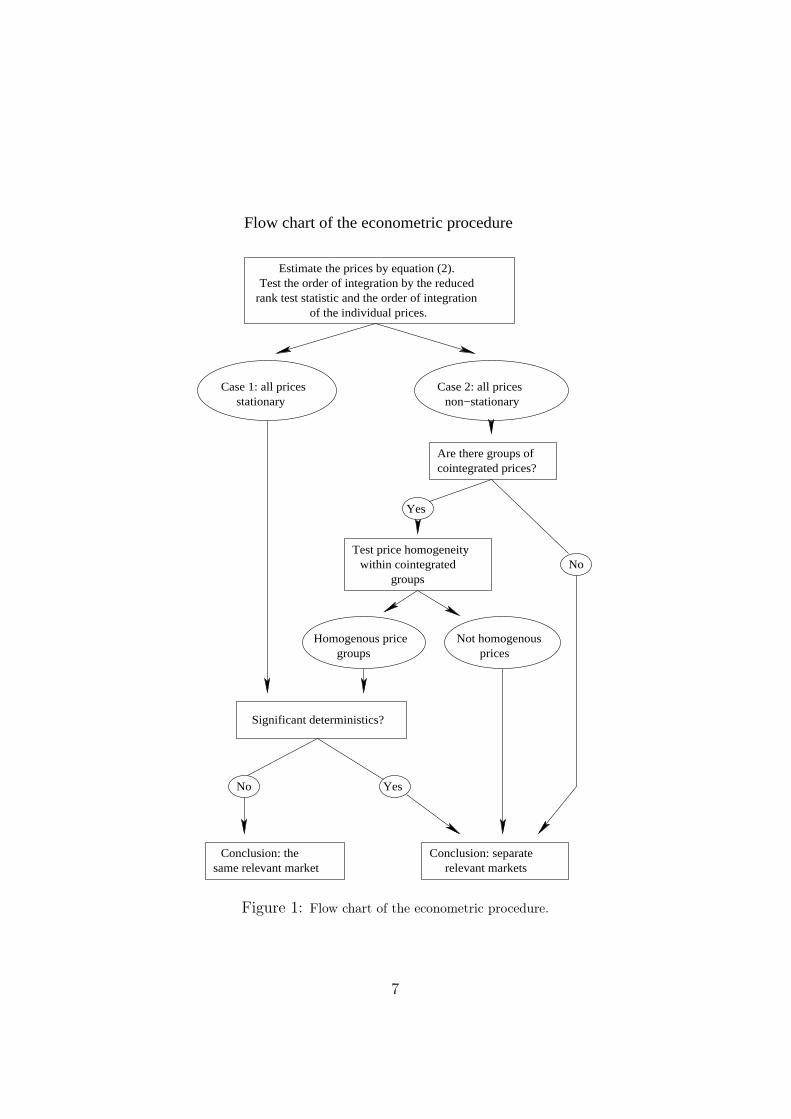
We can summarize our econometric procedure, whereby the relevant mar-ket is defined, in a logical sequence of steps. In the first step we determinewhether the price series are stationary or not since the statistical inferenceis crucially dependent on this property. If the prices are stationary andsignificantly correlated, we must control for possible common factors and in-vestigate their relative deterministic differences in order to decide if the areasbelong to the same market. On the other hand, if prices are non-stationary,mean reversion around their combined deterministic components can onlyoccur if they are cointegrated.8 Thus, only if the prices are cointegrated,homogeneous and do not differ significantly with respect to their determin-istic differences can we can conclude the firms belong to the same relevantmarket. Figure 1 summarizes this procedure. We apply this procedure to

8In the intermediate case where one price is stationary while the other is not, therecannot by definition be any mean reversion between the series. Thus, such a result would

6

Flow chart of the econometric procedure

Yes

same relevant marketConclusion: the

relevant marketsConclusion: separate

No

YesNo

Case 1: all pricesstationary non−stationary

Case 2: all prices

pricesgroupsNot homogenousHomogenous price

groupswithin cointegrated

Test price homogeneity

cointegrated prices?Are there groups of

rank test statistic and the order of integration

Estimate the prices by equation (2).

Significant deterministics?

Test the order of integration by the reduced

of the individual prices.

Figure 1: Flow chart of the econometric procedure.

7

characterize the relevant market for production and wholesale of electricityin the Nordic countries in Section 4.

3 The Statistical ModelThe implementation of the econometric approach outlined in the previoussection requires a statistical framework that can be used to analyze the inte-gration and cointegration properties of a vector of prices. A natural choiceis the vector auto-regressive (VAR) model in its error correcting form.

The p-dimensional VAR model with k lags is given by

Xt =k∑

i=1

AiXt−k + ΨDt + εt (1)

where Xt is a p-dimensional time series vector, Ai (i = 1, ..., k) and Ψ areparameter matrices, Dt is a p × f matrix that collects the deterministiccomponents, and εt ∼ Np(0, Σ). In our application Xt will be a vectorof prices from areas that potentially belong to the same market. If Xt ∼I(1) (integrated of the first order) it is convenient to transform (1) into itscorresponding error correction form

∆Xt =k−1∑i=1

Γi∆Xt−i + ΠXt−1 + ΨDt + εt (2)

where parameter matrices Γi and Π are functions of the Ai matrices. Theproperties of this model are extensively investigated in Johansen (1995).

Cointegration can be tested as a reduced rank hypothesis on the Π matrix.If the rank, r, of Π is equal to p we can conclude that Xt is stationary, i.e.Xt ∼ I(0). If 0 < r < p, then Xt ∼ I(1) is cointegrated with r cointegrationvectors and p− r common stochastic trends. In this case, Π = αβ′, where αand β are two (p × r) matrices of full column rank. The cointegration spaceis spanned by β′. If r = 0 then Xt ∼ I(1) and the process is not cointegrated.

An important special case of (2) is obtained when 0 < r < p and adeterministic linear trend is restricted to the cointegration space. The reasonfor restricting the linear trend is that (2) implies quadratic trends in Xt

otherwise. If the trend is restricted, ΠXt−1 in (2) can be written as αβ̃′X̃t−1,where β̃ = (β′, κ)′, κ is a r -dimensional vector, and X̃t−1 = (X ′

t−1, t)′.The test for the reduced rank of Π, known as the trace test, was developed

by Johansen (1991). The null hypothesis of the trace test is that the rank of

indicate that the price areas do not belong to the same relevant market.

8

Π is less or equal to r. Hence, the natural testing sequence from a statisticalpoint of view is to start by testing r = 0 and then successively increasing therank by one until the first non-rejection. The likelihood ratio test statistic(trace test) of the hypothesis that the cointegration rank is r or less is givenby

−2logQ(r) = −T

p∑i=r+1

log(1 − λi) (3)

where λi are the eigenvalues of a reduced rank regression and T is the samplesize. Thus, the test will reject if the eigenvalues corresponding to the p − rcommon stochastic trends are statistically far from unity.

Given Π = αβ′ , general linear hypotheses on β can be tested in the form

Hβ : β = (H1ϕ1, ..., Hrϕr) (4)

where Hi(p × (p − mi)) imposes mi restrictions on βi, and ϕi((p − mi) × 1)consists of p−mi freely varying parameters. The likelihood ratio test of thehypotheses is asymptotically χ2. Stationarity of an individual variable in Xt

can be tested by formulating Hi in such a way that one of the β-vectors is aunit vector.

The α-vectors can also be restricted in a similar way. Of special interestis the case where one or several rows in α consist of zeros. A variable witha zero row in α is said to be weakly exogenous. A weakly exogenous vari-able generates a common stochastic trend and is not affected by the otherstochastic trends in the system. In this sense, a weakly exogenous variablecan be viewed as a forcing variable in the long-run.

In our application it will sometimes be more convenient to obtain a rep-resentation of the p− r common stochastic trends rather than the stationaryrelations β when p > 2. The reason is that the common trends represen-tation contain the same statistical information as α and β, but relieves usfrom testing

(p2

)cointegrating combinations between the prices. Instead, the

cointegrating combinations can be directly read from the common trendsrepresentation.9 The inverse of (2), provided by the Granger-Johansen rep-resentation theorem is

Xt = C

t−1∑i=0

(εt + ΨDt) + C(L)(εt + ΨDt) + X0 (5)

where C = β⊥

(α′⊥

(I −

∑k−1i=1 Γi

)β⊥

)−1

α′⊥, C(L) is a stationary matrix

lag-polynomial with zeros outside the unit circle, X0 summarizes the initial9However, cointegration tests can be utilized when the common trends representation

yields ambiguous results.

9

condition, and α⊥ and β⊥ denotes the orthogonal complements to α and β.The is the common trends representation of Xt. The matrix α′

⊥ exhibits the

common stochastic trends, whereas β⊥

(α′⊥

(I −

∑k−1i=1 Γi

)β⊥

)−1

providesthe loadings of the common stochastic trends into each element of Xt.

4 Application to Nord Pool price dataIn this section we apply the econometric approach to price data from theNordic market for production and wholesale of electricity, Nord Pool. WithinNord Pool wholesale prices of electricity are perfectly equalized among firmswithin a given price area. Therefore, rather than considering the prices ofindividual firms we investigate the relevant market delineation among Nordicprice areas instead. We begin by investigating if the price areas Finland andSweden belong to the same relevant market. We then extend the analysis tocover all price areas of Nord Pool.

4.1 Data, Frequency and Aggregation

The data consists of hourly observations on prices from the following NordPool price areas: Finland, Sweden, Norway 1, Norway 2, Norway 3, Den-mark 1, and Denmark 2. In the terminology used by Nord Pool, Norway 1refers to South-Norway (the Oslo area), Norway 2 to mid-Norway (the Trond-heim area), Norway 3 to North-Norway (the Tromsö area), Denmark 1 toEast-Denmark (the Copenhagen area) and Denmark 2 to West-Denmark (theOdense-area). Due to the almost complete correlation between Norway 2 andNorway 3, we only consider Norway 3 in the analysis in order to avoid se-vere multicollinearity problems.10 The price observations cover the period2001:01:01:00-2007:12:31:23, which means that the sample consists of 61337observations in total. Figures 2 and 3 depict the area-specific prices (ag-gregated to a weekly frequency to facilitate the exposure). Table 1 presentsdescriptive evidence on price convergence between Finnish and Swedish pricesduring the period 2001-2007. The correlation coefficient between Finnish andSwedish prices exceeds 0.96 for all years except 2005 and 2006. The meanof the price difference in the original hourly data, P FIN

t − P SWEt , is -0.140

and the corresponding t-value is 5.71. Furthermore, the median of the pricedifference is zero.

The large number of observations causes two particular econometric prob-lems, one computational and the other statistical in nature. The first problem

10Moreover, price data on Norway 2 is only available from 2003:07:23:00 onwards.

10

2001 2002 2003 2004 2005 2006 2007 2008

25

50

75

100 Weekly Finnish Prices

2001 2002 2003 2004 2005 2006 2007 2008

25

50

75

100 Weekly Swedish Prices

2001 2002 2003 2004 2005 2006 2007 2008

50

100Weekly Norwegian Area 3 Prices

Figure 2: Weekly price aggregates for Nord Pool price areas Finland, Sweden, andNorway 3.

Finnish and Swedish Prices: Correlation and Price Differences2001 2002 2003 2004 2005∗) 2006 2007

Corr(P FINt , P SWE

t ) 0.998 0.967 0.984 0.970 0.783 0.852 0.988P FIN

t 22.84 27.27 35.30 27.68 30.53 48.57 30.01P SWE

t 22.86 27.61 36.49 28.08 29.76 48.12 30.26P FIN

t − P SWEt -0.02 -0.34 -1.18 -0.40 0.77 0.45 -0.25

Table 1: Finnish vs Swedish area prices (in Euro). *) A two hour price spike at 8.12.2005which is fully due to Svenska Kraftnät’s operation is removed from the data.

11

2001 2002 2003 2004 2005 2006 2007 2008

50

100 Weekly Norwegian Area 1 Prices

2001 2002 2003 2004 2005 2006 2007 2008

25

50

75Weekly Danish Area 1 Prices

2001 2002 2003 2004 2005 2006 2007 2008

25

50

75

100 Weekly Danish Area 2 Prices

Figure 3: Weekly price aggregates for Nord Pool price areas Norway 1, Denmark 1 andDenmark 2.

arises as the computational power of modern PCs is simply not sufficient tocalculate the trace test statistic for a well-specified model of the hourly data.The second problem is that the large number of observations associated withthe hourly frequency increases the power of virtually all statistical tests (seefor example Otero and Smith (2000)). Of particular concern in this contextis that the increase in power associated with the hourly frequency wouldtend to create a bias towards the conclusion that the price areas belong tothe same relevant market. In this study we are particularly concerned witherrors of type I, i.e. we want to avoid defining the market too broadly. Fur-thermore, with hourly observations it is difficult to account for all exogenousevents that cause symmetric additive outliers in the price series. Such out-liers can cause an additional bias towards cointegration or even stationarity(see Bohn Nielsen (2004) and Franses and Haldrup (1994), among others).

From a statistical point of view temporal aggregation reduces the powerof the tests and makes the problem with outliers manageable. The reasonis that averaging over periods preserves the integration and cointegrationproperties of the data while reducing the total sample size T (see Marcellino,1999). Thus, we will mainly operate with daily aggregates of the price datain this paper. However, we conduct robustness checks with both weekly and

12

2005

100

200

300 Hourly Finnish Prices

2005

25

50

75

100

125Daily Finnish Prices

2005

25

50

75

100 Weekly Finnish Prices

2005

20

40

60

Monthly Finnish Prices

Figure 4: Hourly, Daily, Weekly, and Monthly aggregates of Finnish prices.

monthly frequencies. Moreover, to the extent that results are obtainable withhourly observations these essentially coincide with the results based on dailyobservations.

The number of observations for each price area at the daily frequency is2556. Figure 4 shows Finnish area prices at different frequencies of aggrega-tion (hourly, daily, weekly and monthly). While the aggregation, of course,reduces the short-term volatility, the long-run stochastic trend is invariantto aggregation, as Figure 4 graphically supports.

4.2 Tests with Finnish and Swedish Prices

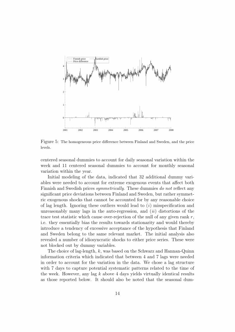
We begin by applying our procedure to Finnish and Swedish prices. Figure 5presents a graphical exposition of the daily electricity prices (logarithms) inFinland and Sweden for the period 2001-2007 as well as the homogeneousprice difference pFIN

t − pSWEt . This figure shows a very high correlation

between the prices in Finland and Sweden. In fact, the correlation is so highthat for most of the time it is optically impossible to distinguish the Finnishprice from the Swedish price.

The (logs of) Finnish and Swedish prices, pFINt and pSWE

t , are modeledby (2), where a trend is restricted to the cointegration space. We add 6

13

2001 2002 2003 2004 2005 2006 2007 2008

0

1

2

3

4

Finnish price Price difference

Swedish price

Figure 5: The homogeneous price difference between Finland and Sweden, and the pricelevels.

centered seasonal dummies to account for daily seasonal variation within theweek and 11 centered seasonal dummies to account for monthly seasonalvariation within the year.

Initial modeling of the data, indicated that 32 additional dummy vari-ables were needed to account for extreme exogenous events that affect bothFinnish and Swedish prices symmetrically. These dummies do not reflect anysignificant price deviations between Finland and Sweden, but rather symmet-ric exogenous shocks that cannot be accounted for by any reasonable choiceof lag length. Ignoring these outliers would lead to (i) misspecification andunreasonably many lags in the auto-regression, and (ii) distortions of thetrace test statistic which cause over-rejection of the null of any given rank r,i.e. they essentially bias the results towards stationarity and would therebyintroduce a tendency of excessive acceptance of the hypothesis that Finlandand Sweden belong to the same relevant market. The initial analysis alsorevealed a number of idiosyncratic shocks to either price series. These werenot blocked out by dummy variables.

The choice of lag-length, k, was based on the Schwarz and Hannan-Quinninformation criteria which indicated that between 4 and 7 lags were neededin order to account for the variation in the data. We chose a lag structurewith 7 days to capture potential systematic patterns related to the time ofthe week. However, any lag k above 4 days yields virtually identical resultsas those reported below. It should also be noted that the seasonal dum-

14

Reduced rank hypothesis, Xt = (pFINt , pSWE

t )′

Sample r = 0 r = 1λi Tr Tr95 p-val λi Tr Tr95 p-val

Full sample, 01-07 0.055 153.04 25.73 0.000 0.003 9.34 12.45 0.164Half sample, 04-07 0.056 88.74 25.73 0.000 0.003 4.67 12.45 0.649Year 01 0.098 56.17 25.73 0.000 0.052 19.09 12.45 0.003Year 02 0.081 38.97 25.73 0.000 0.024 8.86 12.45 0.194Year 03 0.097 58.92 25.73 0.000 0.061 22.49 12.45 0.001Year 04 0.069 33.93 25.73 0.003 0.023 8.31 12.45 0.234Year 05 0.097 50.48 25.73 0.000 0.038 13.97 12.45 0.026Year 06 0.079 33.93 25.73 0.003 0.013 4.68 12.45 0.648Year 07 0.061 31.00 25.73 0.009 0.024 8.56 12.45 0.215

Table 2: The reduced rank test statistic for daily Finnish and Swedish prices. In thetable, λi are the eigenvalues from the reduced rank regression, Tr is the trace test statistic,Tr95 is the 95%-quantiles of the trace distribution, and p-val is the probability valuesassociated with the null hypothesis of the given rank in the columns. Bold values indicateinsignificant results at a 1% significance level.

mies accounting for monthly variation were all insignificant, and thereforeexcluded.

With these choices, we tested the model for long-run structural stability.11There were some indications of a structural shift in the middle of year 2003.For this reason, we consider both the full sample (2001-2007), and the latterhalf of the sample (2004-2007). In addition, we consider each year separatelyas a robustness check.12

4.2.1 Cointegration tests on Finnish and Swedish prices

Table 2 reports the rank test statistic for the different samples. Since weare worried about errors of type I, we choose to conduct the test at the1% significance level. Table 2 reveals that r = 0 is rejected in all samples(although, in year 2007 we are close to non-rejection). Moreover, apart fromthe relatively stable years 2001 and 2003, we cannot reject the null hypothesisof r = 1. These results suggest that there is one common stochastic trend in

11The tests of structural include constancy tests for the coefficient estimates of the iden-tified cointegration space, constancy of the log-likelihood, and constancy of the canonicalcorrelations λi, among others. These tests are described in Hansen and Johansen (1999).

12It should be noted that a year is in general a very short period within which toinvestigate the long-run properties of time series, i.e. integration and cointegration. Thus,results may differ to some extent from year to year.

15

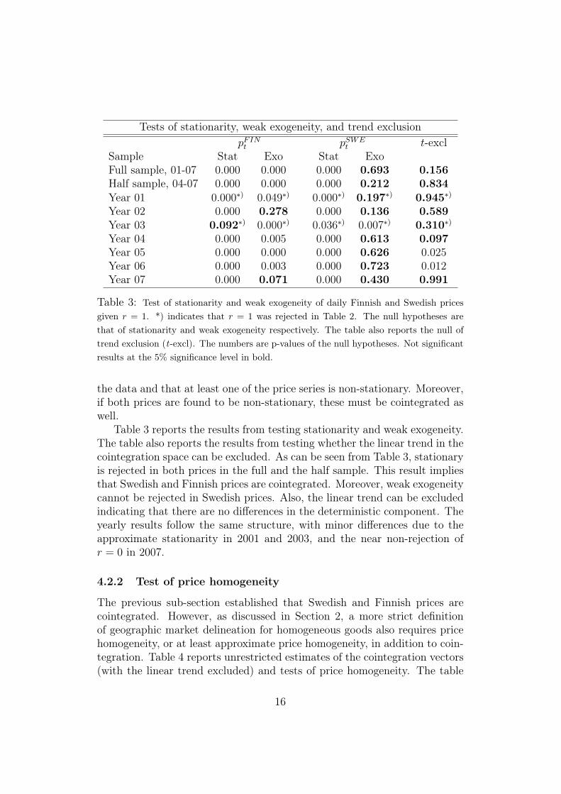
Tests of stationarity, weak exogeneity, and trend exclusionpFIN

t pSWEt t-excl

Sample Stat Exo Stat ExoFull sample, 01-07 0.000 0.000 0.000 0.693 0.156Half sample, 04-07 0.000 0.000 0.000 0.212 0.834Year 01 0.000∗) 0.049∗) 0.000∗) 0.197∗) 0.945∗)

Year 02 0.000 0.278 0.000 0.136 0.589Year 03 0.092∗) 0.000∗) 0.036∗) 0.007∗) 0.310∗)

Year 04 0.000 0.005 0.000 0.613 0.097Year 05 0.000 0.000 0.000 0.626 0.025Year 06 0.000 0.003 0.000 0.723 0.012Year 07 0.000 0.071 0.000 0.430 0.991

Table 3: Test of stationarity and weak exogeneity of daily Finnish and Swedish pricesgiven r = 1. *) indicates that r = 1 was rejected in Table 2. The null hypotheses arethat of stationarity and weak exogeneity respectively. The table also reports the null oftrend exclusion (t-excl). The numbers are p-values of the null hypotheses. Not significantresults at the 5% significance level in bold.

the data and that at least one of the price series is non-stationary. Moreover,if both prices are found to be non-stationary, these must be cointegrated aswell.

Table 3 reports the results from testing stationarity and weak exogeneity.The table also reports the results from testing whether the linear trend in thecointegration space can be excluded. As can be seen from Table 3, stationaryis rejected in both prices in the full and the half sample. This result impliesthat Swedish and Finnish prices are cointegrated. Moreover, weak exogeneitycannot be rejected in Swedish prices. Also, the linear trend can be excludedindicating that there are no differences in the deterministic component. Theyearly results follow the same structure, with minor differences due to theapproximate stationarity in 2001 and 2003, and the near non-rejection ofr = 0 in 2007.

4.2.2 Test of price homogeneity

The previous sub-section established that Swedish and Finnish prices arecointegrated. However, as discussed in Section 2, a more strict definitionof geographic market delineation for homogeneous goods also requires pricehomogeneity, or at least approximate price homogeneity, in addition to coin-tegration. Table 4 reports unrestricted estimates of the cointegration vectors(with the linear trend excluded) and tests of price homogeneity. The table

16

Unrestricted estimates and test of price homogeneitySample Unrestricted estimates test of pFIN

χ2(df) p-valFull sample, 01-07 pFIN

t − 0.97(−102.35)

· P SWE χ2(1) = 7.26 0.007

Half sample, 04-07 pFINt − 0.99

(−75.17)· P SWE χ2(1) = 0.14 0.706

Year 01∗) pFINt − 0.97

(−137.65)· P SWE χ2(1) = 7.21 0.007

Year 02 pFINt − 0.90

(−45.64)· P SWE χ2(1) = 12.84 0.000

Year 03∗) pFINt − 0.74

(−15.77)· P SWE χ2(1) = 8.99 0.003

Year 04 pFINt − 0.89

(−23.75)· P SWE χ2(1) = 4.10 0.043

Year 05 pFINt − 1.07

(−17.69)· P SWE χ2(1) = 0.73 0.391

Year 06 pFINt − 0.96

(−24.99)· P SWE χ2(1) = 0.90 0.342

Year 07 pFINt − 0.95

(−76.65)· P SWE χ2(1) = 9.39 0.002

Table 4: Unrestricted estimates of the cointegration vector between Finnish and Swedishprices in each sample (the linear trend is excluded), given r = 1. *) indicates that r = 1 wasrejected in Table 2. The numbers in parenthesis are t-values. The last two columns testhomogeneity between the prices. Bold values indicate non-rejection at the 5% significancelevel.

reveals that there is a tendency for Swedish prices to be somewhat higherthan the Finnish prices. Furthermore, we note that price homogeneity can-not be rejected in the half sample (2004-2007) and that the prices are neverfar from homogeneity in any of the other samples.

4.2.3 Conclusions

Our econometric test, conducted in line with the procedure summarized inFigure 1, justify the following conclusions.

1. Finnish and Swedish prices are integrated (of the first order).

2. Finnish and Swedish prices are cointegrated and nearly homogeneous.

3. The deterministic linear trend in the price difference is insignificant.

Consequently, our econometric test supports the view that Finland and Swe-den constitute the same relevant market for production and wholesale of

17

electricity. Furthermore, Swedish prices are (long-run) weakly exogenous in-dicating that in a structural sense the Swedish price area acts as a priceleader relative to the Finnish area. The Swedish prices tend to be somewhatmore volatile (in the long run) than the Finnish prices.

4.2.4 Robustness

We conducted the reduced rank test statistic on weekly (365 observations)and monthly aggregates (84 observations). We consistently found that r = 0was rejected, whereas r = 1 could not be rejected. Moreover, we foundthat Swedish prices where weakly exogenous in the lower frequencies as well.Overall, these results are consistent with the results associated with the dailyfrequency.

We also obtained some results of interest for the hourly frequency. Therank test statistic was not computationally available for a well-specifiedmodel of the hourly data (including sufficient lags and dummies for sym-metric outliers etc.). However, auxiliary information such as the roots of thecompanion matrix and the t-values of the α-matrix support r = 1 in thehourly sample as well. Conditional on this choice of rank (r = 1), we againfound that Swedish prices were weakly exogenous with respect to Finnishprices. In addition, we calculated the half-lives implied by the estimatedspeed of the equilibrium adjustment of Finnish prices (first α coefficient).These indicated that an average equilibrium shock to the price differencedissipates in slightly less than four hours. Overall, the results associatedwith hourly data are consistent with the conclusions reported for daily data.

4.3 Is the Relevant Market More Extensive than Fin-land and Sweden?

So far our analysis has been restricted to Finland and Sweden. However,Nord Pool defines an integrated market design for a significantly larger areacomprising price areas Norway 1, Norway 2, Norway 3, Denmark 1 and Den-mark 2, in addition to Finland and Sweden. We now extend our analysis towhole Nord Pool area.

On the Nord Pool level we report the results from the full sample (2001-2007) and the latter half sample (2004-2007). We do not report individualyears, but emphasize that the yearly samples follow similar patterns. In ad-dition, we also report the results from the full sample excluding the year2007 (i.e. the sample 2001-2006). The reason is that the hydro reservoirlevel in Norway 1 was close to the maximum level during 2007, thereby in-ducing an extremely high supply of electricity generated by hydro power in

18

0 5 10 15 20 25 30 35 40 45 50

30

40

50

60

70

80

90Average 1990−2000 2007

Figure 6: Norway 1 (South Norway) hydro reservoir content (% of full) in year 2007compared with a historical average (1990-2000).

order to avoid wastes (see Figure 6). This production exceeded the exporttransmission capacity of Norway 1, thereby leading, by necessity, to substan-tially lower prices in Norway 1 compared to the other Nord Pool areas, inparticular during the latter half of 2007 (see Figure 7). It turns out thatthe price deviation in 2007 was sufficiently large and persistent to induce acharacterization of Norway 1 as a separate relevant market whenever 2007 isin the sample, as is discussed below. Thus, by excluding 2007 from the fullsample we can assess the effect of this particular year on the overall results.As before, we label the logarithms of the prices in the different areas as pFIN

t ,pSWE

t , pNOR1t , pNOR3

t , pDK1t and pDK2

t respectively.On the Nord Pool level the prices were modeled by (2), where a trend

was included in the cointegration space and identical seasonal dummies wereadded as before. In a similar fashion as before, 33 dummy variables wereadded to account for extreme exogenous events that affected at least twoor more areas symmetrically. As earlier, at least four lags were needed toaccount for the variation in the data. Following our procedure for the analysisof Finland and Sweden we selected the lag structure with k = 7.

19

2001 2002 2003 2004 2005 2006 2007 2008

−1

0

1

2Difference of Finnish and Norwegian Area 1 Prices

2001 2002 2003 2004 2005 2006 2007 2008

−1

0

1

2 Difference of Finnish and Norwegian Area 3 Prices

Figure 7: The homogeneous price difference between Finland and Norway area 1 (uppergraph), and between Finland and Norway area 3 (lower graph).

4.3.1 Cointegration tests on Nord Pool prices

The reduced rank hypothesis is reported in Table 5. Table 5 indicates that therank in the full sample is five, independently of whether 2007 is excluded ornot. This implies that all non-stationary Nord Pool prices are cointegrated,because they share the same stochastic trend. Hence, the non-stationaryarea-specific prices cannot evolve independently of each other. In other wordsthese price areas impose competitive discipline on each other. The table alsoshows that the rank is four in the half sample. Given that the area-specific

Reduced rank hypothesis, Xt = (pFINt , pSWE

t , pNOR1t , pNOR1

t , pDK1t , pDK1

t )′

r = 0 r = 1 r = 2 r = 3 r = 4 r = 5Full sample, 01-07 0.000 0.000 0.000 0.000 0.003 0.47Half sample, 04-07 0.000 0.000 0.000 0.000 0.187 0.734Full sample, 01-06 0.000 0.000 0.000 0.000 0.000 0.682

Table 5: The reduced rank test statistic for Nord Pool prices. The numbers are p-valuesof the null hypothesis of the ranks given in the columns. Not significant results at the 1%significance level in bold.

20

Tests of stationarity and weak exogeneitySample r Test pFIN

t pSWEt pNOR1

t pNOR3t pDK1

t pDK2t

Full sample, 01-07 5 Stat 0.000 0.000 0.000 0.000 0.000 0.000Exo 0.000 0.000 0.004 0.532 0.000 0.000

Half sample, 04-07 4 Stat 0.000 0.000 0.000 0.000 0.000 0.000Exo 0.000 0.000 0.197 0.316 0.000 0.000

Full sample, 01-06 5 Stat 0.000 0.000 0.000 0.000 0.000 0.000Exo 0.000 0.000 0.112 0.014 0.000 0.000

Table 6: Test of stationarity and weak exogeneity of daily Nord Pool prices given r = 1.The null hypotheses are that of stationarity and weak exogeneity respectively and thenumbers are p-values of the null hypotheses. Not significant results at the 5% significancelevel in bold.

prices are non-stationary, the case with a rank r = 4 would facilitate aninterpretation according to which Nord Pool can be decomposed into at leasttwo separate relevant markets. We demonstrate below that the additionalunit-root originates in the extreme conditions in Norway 1 during 2007.

Table 6 reports the results of testing stationarity and weak exogeneity onall area-specific prices in the samples. Table 6 shows that stationarity can berejected for all area-specific prices, regardless of sample (the time horizon) orchoice of rank. Thus, for the full samples 2001-2007 and 2001-2006 the pricesin all Nord Pool areas are cointegrated. Furthermore, in the half sample theNord Pool area prices can potentially be divided into three groups accordingto whether they exclusively share one of the two stochastic trends or whetherthey contain both trends. Interestingly, pNOR3

t is weakly exogenous in the fullsample when 2007 is included, whereas pNOR1

t is weakly exogenous when 2007is excluded. Both pNOR1

t and pNOR3t are weakly exogenous is the half sample.

These results suggest that Norway 1 acts as the price leader under normalconditions, like those prevailing when year 2007 is excluded. However, duringthe abnormal year 2007, when the export transmission capacity of Norway 1was exceeded, the role of price leader was taken over by Norway 3. Under allcircumstances, the two Norwegian areas serve as price leaders relative to allother price areas in Nord Pool. Moreover, exclusion of the restricted lineartrend could not be rejected regardless of the sample or the choice of rank.

4.3.2 Tests of price homogeneity

The system approach adopted in this paper allows for simultaneous tests ofprice homogeneity between two or more Nord Pool price areas. It seemsnatural to begin by conducting pairwise tests and subsequently to extend

21

Stochastic trends and their loadingsFull sample, 01-07 Half Sample, 04-07 Full sample, 01-06

r = 5 r = 4 r = 5∑ti=1 εNOR3

i

∑ti=1 εNOR3

i

∑ti=1 εNOR1

i

∑ti=1 εNOR1

i

pFINt 0.523

(4.250)0.469(6.568)

0.020(0.793)

0.381(4.969)

pSWEt 0.544

(4.250)0.485(6.709)

0.010(0.388)

0.403(4.969)

pNO1t 0.729

(4.250)−0.182(−1.243)

0.768(14.530)

0.436(4.969)

pNO3t 0.566

(4.250)0.489(6.487)

0.028(1.027)

0413(4.969)

pDK1t 0.335

(4.250)0.221(4.288)

0.116(6.239)

0.191(4.969)

pDK2t 0.489

(4.250)0.381(6.214)

0.039(1.770)

0.355(4.969)

Table 7: Loadings to the stochastic trends in the Norwegian prices. The numbers inparenthesis are t-values.

the tests by successively adding more areas. Much effort can be saved byinvestigating the loadings of the common stochastic trends (see equation(5)) prior to formally testing price homogeneity, since price pairs that arevery far from homogeneity are easily detected that way.

Given the weak exogeneity results we know that the common stochas-tic trends, α′

⊥∑t

i=1 εi, consist of the two Norwegian prices. Labeling theseas

∑ti=1 εNOR1

i and∑t

i=1 εNOR3i respectively, Table 7 reports the loadings to

each trend. Table 7 reveals that, in the full sample 2001-2007, prices in theNord Pool areas Finland, Sweden, Norway 3 and Denmark 2 have similarloadings. For instance the relative loading between Finland and Sweden iscFIN/cSWE = 0.523/0.544 = 0.96 (see Section 2). Denmark 2 and Norway 3have the smallest relative loading, cDK2/cNO3 = 0.85, which is rather farfrom unity. Norway 1 and Denmark 1 each have significantly different load-ings from the rest. Based on these observations, we only report the testsof price homogeneity within the subset {pFIN

t , pSWEt , pNO3

t , pDK2t }.13 The

upper part of Table 8 reports pairwise tests of price homogeneity. As canbe seen from the table, none of the pairwise tests were rejected, althoughsome price pairs came close to rejection. The lower part of Table 8 reportsthe test of price homogeneity between three or more prices within the subset{pFIN

t , pSWEt , pNO3

t , pDK2t }. The only non-rejections occur for the subsets

{pFINt , pNO3

t , pDK2t } and {pSWE

t , pNO3t , pDK2

t }. However, the other subsets of13The homogeneity tests for other price pairs or groups were rejected. The detailed

results are available upon request.

22

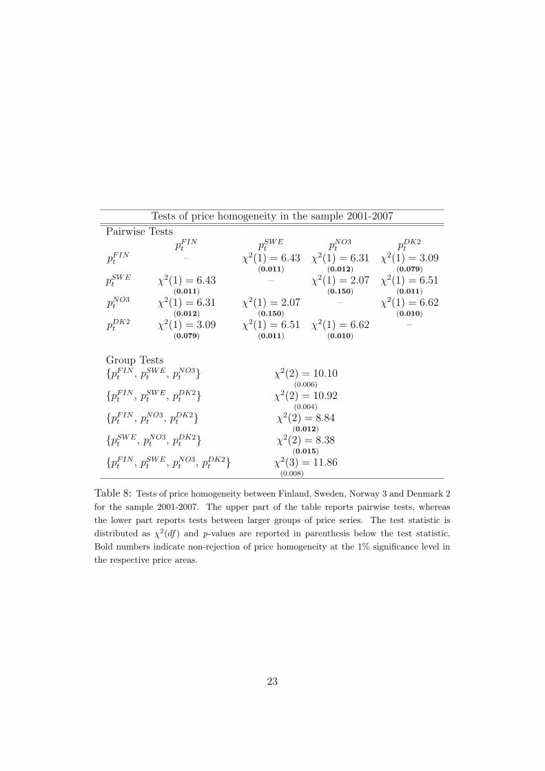
Tests of price homogeneity in the sample 2001-2007Pairwise Tests

pFINt pSWE

t pNO3t pDK2

t

pFINt – χ2(1) = 6.43

(0.011)

χ2(1) = 6.31(0.012)

χ2(1) = 3.09(0.079)

pSWEt χ2(1) = 6.43

(0.011)

– χ2(1) = 2.07(0.150)

χ2(1) = 6.51(0.011)

pNO3t χ2(1) = 6.31

(0.012)

χ2(1) = 2.07(0.150)

– χ2(1) = 6.62(0.010)

pDK2t χ2(1) = 3.09

(0.079)

χ2(1) = 6.51(0.011)

χ2(1) = 6.62(0.010)

–

Group Tests{pFIN

t , pSWEt , pNO3

t } χ2(2) = 10.10(0.006)

{pFINt , pSWE

t , pDK2t } χ2(2) = 10.92

(0.004)

{pFINt , pNO3

t , pDK2t } χ2(2) = 8.84

(0.012)

{pSWEt , pNO3

t , pDK2t } χ2(2) = 8.38

(0.015)

{pFINt , pSWE

t , pNO3t , pDK2

t } χ2(3) =(0.008)

11.86

Table 8: Tests of price homogeneity between Finland, Sweden, Norway 3 and Denmark 2for the sample 2001-2007. The upper part of the table reports pairwise tests, whereasthe lower part reports tests between larger groups of price series. The test statistic isdistributed as χ2(df) and p-values are reported in parenthesis below the test statistic.Bold numbers indicate non-rejection of price homogeneity at the 1% significance level inthe respective price areas.

23

Tests of price homogeneity in the sample 2001-2006

{pFINt , pSWE

t , pNO1t } χ2(2) = 15.78

(0.000)

{pSWEt , pNO3

t , pDK2t } χ2(2) = 6.86

(0.033)

{pFINt , pSWE

t , pNO3t } χ2(2) = 7.31

(0.026)

{pNO1t , pNO3

t , pDK2t } χ2(2) = 19.90

(0.000)

{pFINt , pSWE

t , pDK2t } χ2(2) = 8.87

(0.012)

{pFINt , pSWE

t , pNO1t , pNO3

t } χ2(3) = 19.19(0.000)

{pFINt , pNO1

t , pNO3t } χ2(2) = 18.19

(0.000)

{pFINt , pSWE

t , pNO1t , pDK2

t } χ2(3) = 16.61(0.001)

{pFINt , pNO1

t , pDK2t } χ2(2) = 16.57

(0.000)

{pFINt , pSWE

t , pNO3t , pDK2

t } χ2(3) = 9.03(0.029)

{pFINt , pNO3

t , pDK2t } χ2(2) = 6.98

(0.031)

{pFINt , pNO1

t , pNO3t , pDK2

t } χ2(3) = 20.05(0.000)

{pSWEt , pNO1

t , pNO3t } χ2(2) = 14.79

(0.001)

{pSWEt , pNO1

t , pNO3t , pDK2

t } χ2(3) = 20.32(0.000)

{pSWEt , pNO1

t , pDK2t } χ2(2) = 14.87

(0.001)

{pFINt , pSWE

t , pNO1t , pNO3

t , pDK2t } χ2(4) = 21.34

(0.000)

Table 9: Tests of price homogeneity between Finland, Sweden, Norway 1, Norway 3and Denmark 2 for the sample 2001-2006. The test statistic is distributed as χ2(df) andp-values are reported in parenthesis below the test statistic. Bold numbers indicate non-rejection of price homogeneity at the 1% significance level in the respective price areas.

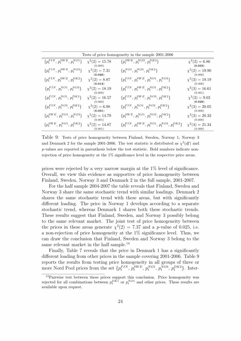
prices were rejected by a very narrow margin at the 1% level of significance.Overall, we view this evidence as supportive of price homogeneity betweenFinland, Sweden, Norway 3 and Denmark 2 in the full sample, 2001-2007.

For the half sample 2004-2007 the table reveals that Finland, Sweden andNorway 3 share the same stochastic trend with similar loadings. Denmark 2shares the same stochastic trend with these areas, but with significantlydifferent loading. The price in Norway 1 develops according to a separatestochastic trend, whereas Denmark 1 shares both these stochastic trends.These results suggest that Finland, Sweden, and Norway 3 possibly belongto the same relevant market. The joint test of price homogeneity betweenthe prices in these areas generate χ2(2) = 7.37 and a p-value of 0.025, i.e.a non-rejection of price homogeneity at the 1% significance level. Thus, wecan draw the conclusion that Finland, Sweden and Norway 3 belong to thesame relevant market in the half sample.14

Finally, Table 7 reveals that the price in Denmark 1 has a significantlydifferent loading from other prices in the sample covering 2001-2006. Table 9reports the results from testing price homogeneity in all groups of three ormore Nord Pool prices from the set {pFIN

t , pSWEt , pNO1

t , pNO3t , pDK2

t }. Inter-14Pairwise test between these prices support this conclusion. Price homogeneity was

rejected for all combinations between pDK1t or pNO1

t and other prices. These results areavailable upon request.

24

estingly, Table 9 reveals that price homogeneity cannot be rejected in anysuch group which excludes the price in Norway 1. On the other hand, pricehomogeneity is always rejected in all groups containing the price in Norway 1.Thus, we have reasons to draw the conclusion that Nord Pool price areas Fin-land, Sweden, Norway 3 and Denmark 2 belong to the same relevant marketin the sample 2001-2006.

In light of data there seems to be a strong relationship between NordPool system prices and deviations of the Nordic (mostly Norwegian) hydroreservoir levels compared with the norm of the year. More precisely, strongreductions in the deviation of the reservoir level relative to norm seem to havedriven the visible incidents of price increases since 2001. Due to restrictionsin transmission capacity between price areas, this price effect is stronger inareas with a higher proportion of hydro generated power.15 This patternis clearly visible in Table 7, where the relative loadings to the stochastictrends are highest for the Norwegian areas, followed successively by Sweden,Finland, and Denmark. This also seems to explain the instances and patternsof deviations from complete price homogeneity. Interestingly, these resultsbear resemblance to the result obtained by Walls (1994) for the U.S. naturalgas industry.

4.3.3 Conclusions

Our econometric test on the whole Nord Pool level, conducted in line withthe procedure in Section 4.2, justify the following conclusions.16

1. All area-specific prices are non-stationary.

2. The area-specific prices are cointegrated with cointegration rank 5 inthe samples 2001-2007 and 2001-2006, whereas is cointegration rank is4 in the sample 2004-2007.

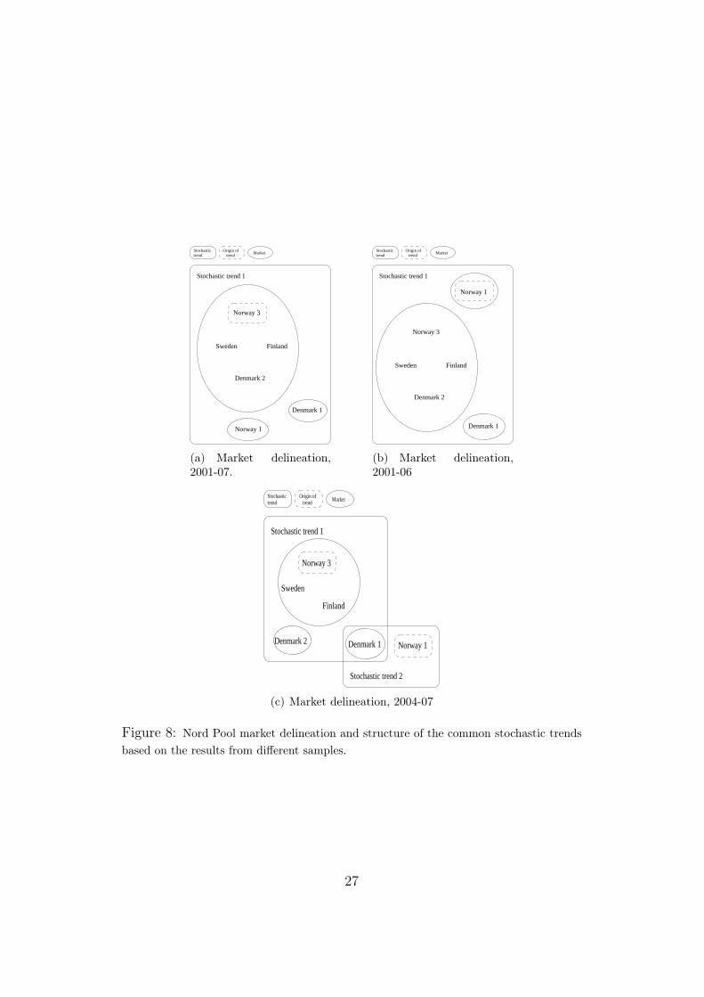
3. During time horizons 2001-2007, as well as 2001-2006, the prices in theNord Pool areas Finland, Sweden, Norway 3, and Denmark 2 share thesame stochastic trends with the same loadings. We draw the unambigu-ous conclusion that the Nord Pool areas Finland, Sweden Norway 3,and Denmark 2 belong to the same relevant market during these peri-ods.

15Hydro power constitutes 98% of the electricity capacity in Norway, 48% in Sweden,18% in Finland, and 0% in Denmark at the end of 2006 (see Nordel annual report andNord Pool).

16As before, we conducted sensitivity analysis with respect to the reduced rank teststatistic on weekly and monthly frequencies. The results where similar to those obtainedon the daily frequency.

25

4. Areas Norway 1 and Denmark 1 define separate markets on their ownduring the periods 2001-2007 and 2001-2006.

5. During the time horizon 2004-2007 the prices areas Finland, Sweden,and Norway 3 belong to the same relevant market. Areas Norway 1,Denmark 1, and Denmark 2 define separate markets on their own.

6. There is a clear tendency that the price areas rich in hydro power serveas price leaders relative to other areas in the same relevant market. Re-strictions in international transmission capacity tend to generate higherprice volatility in these areas relative to the other areas. During normalhydro power conditions (the period 2001-2006), the stochastic trend inprices originates in price area Norway 1. However, if we include theyear 2007 this role is taken over by price area Norway 3.

Figure 8 depicts the decomposition of Nord Pool price areas into differentrelevant markets consistent with the econometric evidence. The figure alsoillustrates the structure of the common stochastic trends in each sample.This market decomposition is reported for the different time horizons 2001-2007, 2004-2007 or 2001-2006. The figure shows that Finland, Sweden, andNorway 3, unambiguously belong to the same relevant market regardless ofthe time horizon. Denmark 2 belongs to this same market in the samples2001-2007 and 2001-2006, but defines its own market in the sample 2004-2007. Norway 1 and Denmark 1 always define their own separate markets.

5 Bottlenecks in the Transmission Capacity be-tween Finland and Sweden

We now return to a detailed investigation of bottlenecks in the transmissioncapacity between Finland and Sweden. During a small proportion of hourswith price differences the international transmission capacity has been insuf-ficient to induce price equalization between Finland and Sweden. Figure 5presents a graphical representation of the frequency by which such price dif-ferences are realized. We refer to such states of nature simply as bottlenecks.Table 10 presents a descriptive yearly account of the number and proportionof hours when there has been a bottleneck in the international transmis-sion capacity between Finland and Sweden. We can observe that during theperiod 2001-2007 there has been a price difference between Finland and Swe-den during 11,47 % of the hours. When there has been a bottleneck in the

26

Norway 3

trendOrigin of

trendMarket

Norway 1

Denmark 1

Stochastic trend 1

Denmark 2

Sweden Finland

Stochastic

(a) Market delineation,2001-07.

Stochastic trend 1

Denmark 1

Stochastictrend

Origin oftrend

Market

Norway 1

Norway 3

Sweden Finland

Denmark 2

(b) Market delineation,2001-06

Stochastic trend 1

Denmark 2

Finland

Sweden

Norway 3

Stochastic trend 2

Stochastictrend

Origin oftrend

Market

Norway 1Denmark 1

(c) Market delineation, 2004-07

Figure 8: Nord Pool market delineation and structure of the common stochastic trendsbased on the results from different samples.

27

Bottleneck Statistics (hours)

2001 2002 2003 2004 2005 2006 2007 2001-2007#{PFIN

t > PSWEt } 30 262 0 0 739 227 44 1301

#{PFINt < PSWE

t } 66 177 2561 2092 77 375 385 5733#{PFIN

t 6= PSWEt } 96 439 2561 2092 816 602 429 7035

#{PFINt = PSWE

t } 8663 8320 6198 6691 7943 8157 8330 54302T 8759 8759 8759 8783 8759 8759 8759 61337

#{P F INt >P SW E

t }T 0.34% 2.99% 0.00% 0.00% 8.44% 2.59% 0.50% 2.12%

#{P F INt <P SW E

t }T 0.75% 2.02% 29.24% 23.82% 0.88% 4.28% 4.40% 9.35%

#{P F INt 6=P SW E

t }T 1.09% 5.01% 29.24% 23.82% 9.32% 6.87% 4.90% 11.47%

#{P F INt =P SW E

t }T 98.91% 94.99% 70.76% 76.18% 90.68% 93.13% 95.10% 88.53%

Table 10: Bottleneck statistics between Finland and Sweden. #{·} denotes the numberof the set and T is the total sample size.

transmission capacity between Finland and Sweden the price difference haspredominantly, during 9,35 % of the hours, been to the advantage of buyersin the Finnish market.

With a definition of the relevant market as national it would, from atheoretical point of view, be logically inconsistent to refer to structural com-petition problems during phases of bottlenecks in the transmission of elec-tricity between Finland and Sweden. The presence of bottlenecks in thetransmission of electricity between Finland and Sweden is an issue, whichis, in principle, unrelated to whether the Finnish market performs well asa national market given the constraints imposed by the Finnish productiontechnology. Bottlenecks in the transmission of electricity between Finlandand Sweden constrain the ability to efficiently exploit the joint supply in thetwo countries, but this does not imply any type of abuse of market power orany other types of strategically induced distortions in the Finnish nationalmarket. Such bottlenecks just mean that consumers are restricted to thenational sources available for electricity generation, and these might not al-ways be able to match the efficiency of the sources available in the othercountry. By logical necessity arguments identifying the bottlenecks of elec-tricity transmission between Finland and Sweden as the core of potentialstructural competition problems imply that the underlying relevant marketis larger than the Finnish national market and incorporate at least Finlandand Sweden. This inconsistency could potentially be reconciled by introduc-ing an intertemporal separation of the relevant market into two phases: thephase when there is no congestion for the transmission of electricity betweenFinland and Sweden and the phase when there is congestion of intercon-

28

nections between these countries.17 In most markets such an intertemporalseparation could not easily be conducted, but the remarkable transparencyof the Nord Pool market for electricity with prices determined regularly andwith high frequency, i.e. every hour, might at least theoretically make suchan intertemporal separation possible. Apparently, the idea behind such anintertemporal separation could then be that the behavior of a potentiallydominant firm in Finland would not be constrained by the competitive dy-namics of the Swedish market during those hours when there is congestionof interconnections.

When evaluating the existing bottleneck statistics the crucial questionis the following: Has the incidence of the fairly infrequent bottlenecks hadany significant price effects? In light of the cointegration analysis conductedin the previous section we can conclude that the incidence of infrequentbottlenecks has induced no such persistent price effects so as to justify aview of Finland and Sweden as defining separate relevant markets. On thecontrary, the cointegration analysis generated evidence in strong support ofFinland and Sweden belonging to the same relevant market even though oureconometric model was designed so as to create a bias in favor of the inferencesupporting separate relevant markets.

Based on hourly area-specific prices one can draw some further descriptiveconclusions regarding the nature of the bottlenecks. The duration of bottle-necks has predominantly been very short, typically one hour or at most a fewconsecutive hours. There is no significant relationship between the hour ofthe day or the weekday and the incidence of a bottleneck. Furthermore, thereis no evidence that the bottlenecks would occur more frequently during thewinter months with the yearly regular peak in demand. As a matter of fact, ifthe winter period is defined as December-March the average frequency of bot-tlenecks is 0,7 % (9,9 %) during the winter months 2001-2005 in associationwith those bottlenecks when the Finnish (Swedish) price exceeds the Swedish(Finnish) price.18 Thus, available data does not support the view with bot-tlenecks emerging as a demand-driven phenomenon. Instead the variations inhydro inflow and the complexity associated with the intertemporal reservoirmanagement together with other stochastic disturbances in the power gener-ation seem to be the primary explanations for the emergence of bottlenecks.Overall, in light of the detailed bottleneck statistics it does not seem crediblethat the states with bottlenecks emerge in a way which is predictable to the

17As pointed out in our introduction, such an intertemporal separation has been sug-gested by the Finnish Competition Authority.

18This should be compared with the yearly frequency of of bottlenecks reported inTable 10. The average frequency of bottlenecks with the Finnish (Swedish) price exceedingthe Swedish (Finnish) price during 2001-2005 was 2,3 % (11,3 %).

29

market participants. Furthermore, these states are typically not of such aduration so as to have antitrust implications.

An intertemporal separation in the definition of the relevant market wouldhave far-reaching consequences for the implementation of competition lawand for competition policy more generally. The same argument in supportof an intertemporal separation of the definition of the relevant market couldthen be applied in all markets characterized by the combination of demandfluctuations and capacity constraints. Such a policy would easily give incen-tives for firms to establish excess capacity so as to avoid the risk of beingaccused of abusing a dominant position in a phase where a bottleneck is re-alized, i.e. a phase where demand exceeds the available capacity. For thatreason such a competition policy would induce distortions with excess ca-pacity and thereby not promote efficient investments. In this respect suchan intertemporal separation of the electricity market into an hour-by-hourmarket would most likely counteract the overall goal of competition policyas a structural microeconomic policy tool with the objective of promotingefficiency in the long run.

6 Concluding CommentsIn this study we applied cointegration analysis to daily aggregates of hourlyprice observations during the period 2001-2007 in the Nord Pool price areaswith the objective of empirically characterizing the geographical dimension ofthe relevant market for production and wholesale of electricity in the Nordiccountries. We initially established econometrically that Finland and Swe-den belong to the same relevant market by demonstrating that Finnish andSwedish area prices are cointegrated and homogeneous. We subsequently ex-tended our analysis to the whole Nord Pool area and were able to establisheconometrically that the price areas Finland, Sweden and Norway 3 unam-biguously belong to the same relevant market. Furthermore, we found thatthe price area Denmark 2 belongs to this same market when evaluated overthe periods 2001-2007 or 2001-2006, but defines its own market over the pe-riod 2004-2007. Norway 1 and Denmark 1 define separate relevant marketson their own for each of the time periods studied. We also found a cleartendency that the price areas rich in hydro power serve as price leaders rela-tive to other areas in the same relevant market. During normal hydro powerconditions (the period 2001-2006), the stochastic trend in prices originates inprice area Norway 1. However, if we include the year 2007 this role is takenover by price area Norway 3.

We presented detailed hourly statistics of bottlenecks in the international

30

transmission capacity between Finland and Sweden in order to evaluate thecompetition policy option of an intertemporal separation in the definition ofthe relevant market into two phases depending on whether restrictions in theinternational transmission capacity prevents the operation of competition.We argued that such an intertemporal separation of the electricity marketinto an hour-by-hour market would most likely counteract the overall goalof competition policy as a structural microeconomic policy tool with the ob-jective of promoting efficiency in the long run. And, under all circumstancesin light of the econometric evidence such an intertemporal separation of therelevant markets is not consistent with the persistency requirements imposedby the SSNIP-test.

The frequency for the emergence of bottlenecks in the transmission ofelectricity between countries is largely determined by the capacity of inter-connections between these countries. A proper structural assessment of therelevant market should not be restricted to past and present market perfor-mance, but it should also take the likely and foreseeable future developmentof the relevant industry into account. In particular, the significance of theproblem with bottlenecks should also be evaluated in light of existing com-mitments and plans for future capacity expansions of the interconnectionsbetween countries.

The transmission system operators in the Nordic countries (Denmark,Finland, Iceland, Norway and Sweden) manage and coordinate the invest-ments into capacity of transmission of electricity between the Nordic coun-tries within the framework of NORDEL. The export capacity from Sweden toother Nordic countries is in total 8010 MW, out of which 2230 MW towardsFinland. Similarly, the interconnection capacity from Finland to other Nordiccountries is 1930 MW, out of which 1830 MW is an export connection to Swe-den. The total export and import capacities for Sweden are fairly equal, 9210MW and 9470 MW, respectively. For Finland the total existing capacity forimport, 4240 MW, substantially exceeds the capacity for export, 2280 MW.Furthermore, total Nordic capacity for imports from other countries (Russia,Estonia, Poland and Germany) is 4710 MW, whereas the interconnection ca-pacity for Nordic electricity export to the same non-Nordic countries is 3550MW. In light of these capacities together with planned investments to furtherimprove the interconnections between national markets we can conclude thateffort is made in order to control the incidence of bottlenecks. Borensteinet al. (2000) present an interesting and relevant theoretical analysis, designedprimarily with the Californian market in mind, of the transmission capacitynecessary for two local markets to achieve the benefits of competition withinthe framework of an integrated market. It is also an overall goal of Europeanenergy policy to promote an expansion of international interconnections in

31

order to support a development in a direction towards the development withthe ultimate goal of creating a European market for production and whole-sale of electricity. Of course, the likely transformation towards a unifiedEuropean market for production and wholesale of electricity will successivelyenlarge the relevant market towards a European level.

Discussions of international interconnection capacity are easily biased to-wards a view according to which higher interconnection capacity always gen-erates benefits. However, it should be kept in mind that it is not sociallyoptimal to establish such an extensive interconnection capacity that the prob-ability for the emergence of a bottleneck would be reduced to zero. As al-ways, the socially optimal capacity is determined by the condition that theexpected marginal social benefit of an additional incremental unit of capac-ity is equal to its marginal social cost. Our characterization of the relevantmarkets within the framework of Nord Pool identifies those price areas forwhich an extended transmission capacity might have particularly high bene-fits. From an overall Nordic perspective high export transmission capacitiesfrom Norway seem particularly valuable in light of our study.

ReferencesBohn Nielsen, H., 2004. Cointegration analysis in the presence of outliers.

Econometrics Journal 7, 249–271.

Borenstein, S., Bushnell, J., Stoft, S., 2000. The competitive effects of trans-mission capacity in a deregulated electricity industry. The RAND Journalof Economics 31, 294–325.

Forni, M., 2004. Using Stationarity Tests in Antitrust Market Definition.American Law and Economics Review 6, 441–464.

Franses, P., Haldrup, N., 1994. The Effects of Additive Outliers on Tests forUnit Roots and Cointegration. Journal of Business & Economic Statistics12 (4), 471–478.

Hansen, H., Johansen, S., 1999. Some tests for parameter constancy in coin-tegrated VAR-models. Econometrics Journal 2 (2), 306–333.

Horowitz, I., 1981. Market Definition in Antitrust Analysis: A Regression-Based Analysis. Southern Economic Journal 48, 1–16.

Johansen, S., 1991. Estimation and Hypothesis Testing of Cointegration Vec-tors in Gaussian Vector Autoregressive Models. Econometrica 59, 1551–1580.

32

Johansen, S., 1995. Likelihood-Based Inference in Cointegrated Vector Auto-Regressive Models. Oxford University Press.

Marcellino, M., 1999. Some Consequences of Temporal Aggregation in Em-pirical Analysis. Journal of Business & Economic Statistics 17 (1), 129–136.

Otero, J., Smith, J., 2000. Testing for cointegration: power versus frequencyof observation - further Monte Carlo results. Economics Letters 67, 5–9.

Slade, M., 1986. Exogeneity Tests of Market Boundaries Applied toPetroleum Products. The Journal of Industrial Economics 34, 291–303.

Spiller, P., Huang, C., 1986. On the Extent of the Market: Wholesale Gaso-line in the Northeastern United States. The Journal of Industrial Eco-nomics 35, 131–145.

Stigler, G., Sherwin, R., 1985. The Extent of the Market. Journal of Law andEconomics 28, 555–585.

Uri, N., Rifkin, E., 1985. Geographic Markets, Causality and Railroad Dereg-ulation. The Review of Economics and Statistics 67, 422–428.

Vandezande, L., Meeus, L., Delvaux, B., Van Calster, G., Belmans, R., 2006.Evaluation of Economic Merger Control Techniques Applied to the Euro-pean Electricity Sector. The Electricity Journal 19, 49–56.

Walls, D., 1994. A Cointegration Rank Test of Market Linkages with anApplication to the U.S. Natural Gas Industry. Review of Industrial Orga-nization 9, 181–191.

33