öMmföäflsäafaäsflassflassflas ffffffffffffffffffffffffffffffffffff

Discussion Papers

Long-Run Relationships Between Labor and Capital: Indirect Evidence on the Elasticity of

Substitution

Mikael Juselius Swedish School of Economics, and RUESG, University of

Helsinki, and HECER

Discussion Paper No. 57 April 2005

ISSN 1795-0562

HECER – Helsinki Center of Economic Research, P.O. Box 17 (Arkadiankatu 7), FI-00014 University of Helsinki, FINLAND, Tel +358-9-191-28780, Fax +358-9-191-28781, E-mail info-hecer@helsinki.fi, Internet www.hecer.fi

HECER Discussion Paper No. 57

Long-Run Relationships Between Labor and Capital: Indirect Evidence on the Elasticity of Substitution* Abstract This paper suggests an indirect method for making inference on the parameter region of the elasticity of substitution between capital and labor. The idea is to investigate if the observed behavior of the data is consistent with theoretical relationships that depend on the particular parameter region of the elasticity of substitution. The advantage of this approach is that it allows for more data oriented modeling. Long-run empirical relationships, consistent with a modeling approach for the economy that assumes a CES production function with an elasticity of substitution above one, are established using Finnish manufacturing data JEL Classification: C32, E23, E24, E25, O30, O52. Keywords: Cointegration, Elasticity of Substitution, Production Function, VAR-Model, Labor Markets. Mikael Juselius Department of Economics P.O. Box 17 (Arkadiankatu 7) FI-00014 University of Helsinki FINLAND e-mail: mikael.juselius@helsinki.fi * I gratefully acknowledge the financial support provided by the Yrjö Jahnsson Foundation and the Research Unit on Economic Structures and Growth (University of Helsinki) to carry out this work. I also wish to thank Rune Stenbacka, Erkki Koskela, Heikki Kauppi, Staffan Ringbom and Katarina Juselius for numerous valuable comments and suggestions. I bear sole responsibility for all remaining errors and omissions.

1 Introduction

There has recently been a renewed interest in the functional form of the aggre-gate production function. This development has partly been due to the empiricalobservation that factor shares have not remained constant (see for example Ben-tolila and Saint-Paul (2003)) casting doubts on the validity of the popular Cobb-Douglas specification. More importantly, the revival of growth theory during thelast decade (see Quah (1996) and Solow (1994)) makes the issue topical sinceother functional specifications can lead to different and richer theoretical results.For instance, assuming a more general CES (Constant Elasticity of Substitution)technology allows for endogenous growth (see for instance Jones and Manuelli(1990)) for some parameter values and multiple stable equilibrium configurationswith respect to the labor share for others (see Azariadis (1996)). Also, in a recentpaper Kauppi et al. (2004) establish relationships between capital and labor mar-ket variables by assuming a CES production function coupled with imperfectionsin both labor and product markets.

With CES production functions, the theoretical nature of many models aredependent on the parameter value of the elasticity of substitution1. Attempts atestimating this elasticity for the CES specification have been the focus of someprevious empirical studies. The predominant approach is to estimate economicfirst order conditions directly and then derive estimates of the substitution elas-ticity from the estimated parameters. The seminal contribution in this respect isArrow et al. (1961). Recent contributions are provided by Duffy and Papageor-giou (2000), Chirinko et al. (2004), Klump et al. (2004) and Antras (2004). Inthe study by Duffy and Papageorgiou (2000) a time panel of 82 countries over 28years is used to estimate a CES specification. They find that a CES productionfunction with an elasticity of substitution above one fits the data quite well forthe most developed countries in their sample (including Finland). They do not,however, address the time series problems of the data2. Chirinko et al. (2004)use an extensive time panel containing data on 1860 US firms over 20 years.They are concerned with the potential time series problems of the data. Theirsolution is splitting the period, taking averages over the sub periods and finallydifferencing, essentially collapsing the time dimension. By this technique theyobtain estimates of the elasticity of substitution at around 0.40. Klump et al.(2004) estimate a supply side system using non-linear estimation techniques forUS time series data. They estimate the substitution elasticity at around 0.60.Antras (2004) follows the approach set forth by Berndt (1976) using time seriesdata from the US private sector to estimate the elasticity of substitution. He

1The Cobb-Douglas functional form is a special case of the CES function corresponding tothe case where the elasticity of substitution is equal to one, as is well known. Whether theelasticity of substitution is above or below unity is of special theoretical interest.

2Another problem with using a panel of countries is that it requires strong assumptions onthe similarities of the countries in sample.

1

finds that this parameter is well below unity if one allows for biased technologicalprogress. He also investigates the time series properties of the data and find non-stationarity and cointegration but does not analyze these problems any further.Ripatti and Vilmunen (2001) estimate first order conditions, based on a CESspecification, on Finnish data using non-linear cointegration techniques. Theyfind an elasticity of substitution well below one, but are forced to make somestrong assumptions on the processes of the unobservables in order to obtain theirresults. As a consequence they implicitly restrict the number of common trendsand hence the number of cointegration vectors. Furthermore, their results arederived under the assumption of perfectly competitive capital and labor marketsalthough they allow for monopolistic competition in the product market.

Overall, the evidence on the elasticity of substitution from previous stud-ies is mixed, with estimated values both above and below one3. Klump et al.(2004) suggest that the reasons for these disparities can be attributed to differ-ences in data construction, different a’ priori assumptions about the nature oftechnological change and differences in the methods applied in estimating the pa-rameters of the CES functions. In addition, it seems likely that the technologicalparameters differ substantially across countries (for instance as consequences ofdifferent stages of development and country level specialization in more advancedeconomies). In this case country-specific estimates should be the preferred alter-native. At the macro level this is only possible in a time series framework. How-ever, most estimation strategies based on first order conditions are restrictive inthe sense that it becomes difficult to model non-stationary data in a persuasiveway.

This paper suggests an indirect way of making empirical inference on theparameter region of the elasticity of substitution. The idea is to investigate ifthe observed behavior of the data is consistent with theoretical relationships thatdepend on the particular parameter region of the elasticity of substitution. Thisapproach is applied to Finnish manufacturing time series data. The advantageof this approach is that it is flexible enough to allow for a more data orientedmodeling approach while retaining a firm connection to economic theory4. Thedrawback, however, is that precise parameter estimates cannot be obtained.

To this end, a theoretical relationship between wages and the capital-laborshare and a relationship between the unemployment rate and the interest rate,derived by Kauppi et al. (2004), will be utilized. They show that the nature ofthese relationships depends crucially on the elasticity of substitution. Further-more, the relationships vanish in the Cobb-Douglas case, i.e in the case when the

3An excellent review of the findings in previous studies that estimate the elasticity of sub-stitution is provided in Klump et al. (2004).

4For example, the time series properties of the data can be handled in a convincing way. Fur-thermore, economic theory usually describe long-run (equilibrium) behavior but is silent aboutthe short-run. The present approach makes it possible to model both within a cointegrationframework.

2

elasticity of substitution is one. In particular, the relationship between wages andthe capital-labor share is negative (positive) when the elasticity of substitutionis below (above) one, while the relationship between the unemployment rate andthe interest rate is positive (negative) when the elasticity of substitution is above(below) one. The intuition for these relationships is that the capital stock actsas a strategic commitment device with respect to wage formation and therebyaffecting unemployment. Thus, if it is possible to establish similar long-run5

relationships empirically, it would be consistent with the CES production func-tion (and inconsistent with a Cobb-Douglas technology). Moreover, the natureof the relationships allow us to make predictions on the parameter values of theelasticity of substitution6.

The statistical workhorse utilized in this paper is the cointegrated VAR (Vec-tor Auto-Regression) model (see Johansen (1995)). This model is particularlywell suited since it does not require assumptions on causality and it allows fornon-stationarity in the data and hence for distinguishing between long-run eco-nomic relationships and (i.e. cointegration) and short-run adjustments (see Engleand Granger (1987)). Furthermore, the estimates also provide insights into theprocesses that determine the variables at hand, which is of interest in itself.

The cointegrated VAR model is estimated on quarterly Finnish manufactur-ing data (using an information set that captures the main features of the modelin Kauppi et al. (2004)) over the years 1980:1-2001:4. I find a positive long-run relationship between manufacturing wages and the capital-labor ratio and anegative long-run relationship between the unemployment rate and the interestrate. These results have two implications. First, the Cobb-Douglas productionfunction specification seems to be inappropriate for the case of Finland. As analternative, the CES specification coupled with imperfections in both productand labor markets is more consistent with the observed behavior of the data.Second, the nature of these relationships is broadly consistent with an elasticityof substitution above one. Furthermore, utilizing the methods proposed by Ar-row et al. (1961), I also obtain a crude estimate of the elasticity of substitutionequal to 1.39. Estimates of the processes determining the changes in the manu-facturing output, hours worked in manufacturing, long-term interest rates, andprice inflation are also obtained as byproducts of the analysis.

The paper is organized in the following manner. In section 2 some propertiesof the CES aggregate production function and the most relevant results fromKauppi et al. (2004) are discussed. Section 3 provides a short summary of themain properties of the cointegrated VAR model. Section 4 is concerned with thestatistical analysis of the data. The empirical results are then discussed in section

5The relationship in Kauppi et al. (2004) is derived in the presence of product and labormarket imperfections and should be viewed as describing “long-run” relationships. Hence, theempirical relationship should have the same property.

6Bentolila and Saint-Paul (2003) uses similar indirect arguments to make inference on theparameter value of the elasticity of substitution based on a fitted equation for the labor share.

3

5 and section 6 finally concludes.

2 The CES production function and relation-

ships dependent on the elasticity of substitu-

tion

This section presents two theoretical relationships that depend on the elasticityof substitution, as established in Kauppi et al. (2004). The first relationshipis between wages and the capital-labor share while the second is a relationshipbetween unemployment and the interest rate. These relationships can be utilizedto make empirical inference on the value of the elasticity of substitution. Therelationships are dependent on the assumption of a CES production functionand indeed on imperfections in both product and labor markets. We begin bydiscussing the CES production function and then turn to the results from Kauppiet al. (2004).

2.1 The CES production function

The concept of an aggregate production function is often a useful (theoretical)point of departure. Although this concept is somewhat problematic7, most au-thors assume that the economy’s production technology is represented by some(two factor) production function like

Y = AF (K, L) (1)

where Y is output, K is capital, L is labor and A captures technological progress8.The function F is usually assumed to be twice continuously differentiable and tosatisfy INADA conditions. Since its introduction by Solow (1956), the undoubt-edly most popular choice has been the Cobb-Douglas production function

Y = AKβL1−β (2)

where 0 < β < 1. The popularity of the Cobb-Douglas specification is probablymostly due to its analytical convenience rather than its empirical realism9. A

7The literature on aggregation suggests that the assumption of an aggregate productionfunction might be hard to justify. For a nice overview see Felipe and Fisher (2003).

8In (1) the technological progress is in the Hicks neutral form. However, allowing for biasedtechnological progress may be important in empirical investigations as noted in Antras (2004).

9The Cobb-Douglas functional form is usually motivated by the Kaldor’s ’stylized facts’, forinstance that factor shares have been largely constant (in fact, the Cobb-Douglas productionfunction implies absolutely constant factor shares). However, this is clearly not the case formany economies as demonstrated by Bentolila and Saint-Paul (2003). Also, allowing for biasedtechnological progress makes Kaldor’s ’stylized facts’ consistent with any production functionspecification Antras (2004).

4

considerably more general alternative is provided by the CES production function

Y = γ[βK

σ−1σ + (1− β)L

σ−1σ

] σσ−1 (3)

where σ is the elasticity of substitution and γ plays a similar role as A in (1)and β captures the functional distribution of income. (3) embeds the popularCobb-Douglas form as a special case when σ = 1. As noted in the introductionthis functional form allows for much richer theoretical results, for example incontexts of endogenous growth. Naturally, many other functional forms woulddo as well. However, as the theoretical literature has predominately focused onthe Cobb-Douglas or the CES function the same focus is maintained in this paper.

2.2 Relationships between capital and labor markets

Kauppi et al. (2004) analyze equilibrium wage formation, unemployment andinvestments under the assumptions of product market imperfections a la Dixitand Stiglitz (1977) and a ’right-to-manage’ union bargaining approach to labormarket imperfections. They generalize previous contributions by Blanchard andGiavazzi (2003) and Spector (2004) by assuming a CES production function whichallows them to study the role of investments. Under these assumptions theyestablish the following relationship between wages and the capital-labor share

∂wN

∂k

<=>

0 as

σ < 1σ = 1

1 < σ < s

(4)

where wN is the Nash bargaining solution of the wage rate, k is the capital-labor share (defined as K/L), σ is the elasticity of substitution from the CESproduction function and s > 1 is the elasticity of substitution between productsin a CES-utility function. Thus, s can be viewed as a measure of the degree ofproduct market competition. As can be seen from (4), the relationship betweenwages and the capital-labor share is negative if the the elasticity of substitution isless than one (i.e. gross complementary). In the Cobb-Douglas case, where σ = 1there is no relation between wages and the capital-labor share. If on the otherhand the elasticity of substitution is above one (gross substitutability) but lessthan the elasticity of product demand, the relationship is positive. The intuitionfor these relationships is that the capital stock acts as a strategic commitmentdevice, inducing wage moderation when σ < 1 while the opposite is true whenσ > s > 1. Kauppi et al. (2004) argue that the case where 1 < s < σ is unlikelyto be empirically relevant and hence disregard this particular case.

Kauppi et al. (2004) also establish another useful relationship. Since unem-ployment is positively related to the wage rate and capital is negatively relatedto the rate of interest, unemployment and the rate of interest are either posi-tively or negatively related as well, if the elasticity of substitution is different

5

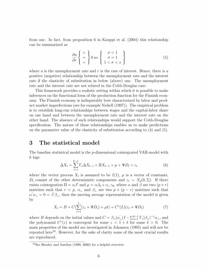
from one. In fact, from proposition 6 in Kauppi et al. (2004) this relationshipcan be summarized as

∂u

∂r

>=<

0 as

σ < 1σ = 1

1 < σ < s

(5)

where u is the unemployment rate and r is the rate of interest. Hence, there is apositive (negative) relationship between the unemployment rate and the interestrate if the elasticity of substitution in below (above) one. The unemploymentrate and the interest rate are not related in the Cobb-Douglas case.

This framework provides a realistic setting within which it is possible to makeinferences on the functional form of the production function for the Finnish econ-omy. The Finnish economy is indisputably best characterized by labor and prod-uct market imperfections (see for example Nickell (1997)). The empirical problemis to establish long-run relationships between wages and the capital-labor shareon one hand and between the unemployment rate and the interest rate on theother hand. The absence of such relationships would support the Cobb-Douglasspecification. The nature of these relationships enables us to make predictionson the parameter value of the elasticity of substitution according to (4) and (5).

3 The statistical model

The baseline statistical model is the p-dimensional cointegrated VAR-model withk lags

∆Xt =k−1∑i=1

Γi∆Xt−i + ΠXt−1 + µ+ ΨDt + εt (6)

where the vector process Xt is assumed to be I(1), µ is a vector of constants,Dt consist of the other deterministic components and εt ∼ Np(0,Σ). If thereexists cointegration Π = αβ′ and µ = αβ0 +α⊥γ0, where α and β are two (p× r)matrixes such that r < p, α⊥ and β⊥ are two p × (p − r) matrixes such thatα′α⊥ = 0 = β

′β⊥, then the moving average representation of the model is given

by

Xt = B + C(t∑

i=1

(εi + ΨDi) + µt) + C∗(L)(εt + ΨDt) (7)

where B depends on the initial values and C = β⊥(α′⊥(I−∑k−1

i=1 Γi)β⊥)−1α⊥, andthe polynomial C∗(z) is convergent for some z < 1 + δ for some δ > 0. Themain properties of the model are investigated in Johansen (1995) and will not berepeated here10. However, for the sake of clarity some of the most crucial resultsare reproduced.

10See Hendry and Juselius (1999, 2000) for a helpful overview.

6

3.1 Linear restrictions on the β-vectors

An important part of the analysis consists of testing linear restrictions on theβ-vectors with the aim of identifying a structure of empirically relevant relations.The restrictions can either be applied to all the cointegrating relations simulta-neously or to the individual vectors separately. Given Π = αβ

′Johansen and

Juselius (1990) show that the same restriction on all the vectors can be tested byformulating the null hypothesis

H0.1 : Π = αϕ′H ′, (8)

that is β = Hϕ, where H is a (p × s) with r ≤ s ≤ p matrix defining linearrestrictions on β. Restrictions on the individual vectors are formulated as

H0.2 :Π = αβ′

β = {H1ϕ1, ... , Hrϕr}(9)

where Hi is p×si, defining linear restrictions on the individual vectors. Johansen(1995) derives the LR-tests for testing the hypothesis in the form (8) and (9).

3.2 Linear restrictions on the α-matrix and weak exogene-ity

The α-vectors can also be restricted in a similar fashion as in the last section.Of special interest is the case where one or several rows in α consist of zeros. Avariable with a zero row in α is not affected by the long-run relationships and ishence treated as weakly exogenous. In this case one estimates

∆X1,t = A∆X2,t +k−1∑i=1

Γi∆Xt−i + αβ′Xt−1 + µ+ ψDt + εt (10)

where X1,t consist of the endogenous variables while X2,t consist of the weaklyexogenous variables and Xt = {X1,t, X2,t}. The dimension is now p− h, where his the number of exogenous variables, Hendry and Juselius (2000).

4 Empirical analysis

The data used in the analysis is Finnish quarterly manufacturing data span-ning over the years 1980:1-2001:4 (88 observations). In accordance with Kauppiet al. (2004), the process determining Finnish manufacturing production, wagesand unemployment is assumed to be described by the information set It ={wt, ut, ct, yt, lt, rt, ∆pt} where wt is real manufacturing wages (log(Wt/P

pt ),

where Wt is a index of manufacturing wages and P pt is the manufacturing pro-

ducer price index), ut is the manufacturing unemployment rate, ct is (the log

7

of) the real capital stock, yt is (the log of) real manufacturing output, lt is (thelog of) hours worked in manufacturing, rt is the nominal yield on government10 year bonds and ∆pt = ∆log(Pt) is the inflation rate. For future reference wealso define the capital labor share, kt, and the output labor share, qt, as the therestrictions kt = ct − lt and qt = yt − lt. The analysis of the long-run relationswas conducted using the computer package CATS in RATS while the short-runstructure was estimated using the computer package PC-Fiml.

4.1 Dynamic long-run relations

The long-run properties (i.e. cointegration relations) of the data were investigatedby estimating model (6) with Xt = [wt, ut, ct, yt, lt, rt, ∆pt]

′, k = 2 and a lineartrend restricted to the cointegration space. The reduced rank hypothesis (tracetest, see Johansen (1995)) is reported in table 1 and indicates that the choiceof rank should be 4 . However, note also that r = 3 is almost accepted at

Table 1: The reduced rank hypothesis. The λi are the eigenvalues correspondingto the estimates of the cointegration vectors.

Ho : r Trace Trace(95) λi

0 217.1 150.3 0.521 154.8 117.5 0.422 108.0 88.6 0.403 64.9 63.7 0.284 37.3 42.8 0.185 20.7 25.7 0.16

the 5% significance level. As a sensitivity precaution, the model was analyzedwith this choice of rank as well, but it did not alter the main results. Givenr = 4, the variables were tested for stationarity, long-run exclusion and weakexogeneity. Stationarity and long-run exclusion were rejected in all variableswhile the capital stock, ct, was found to be weakly exogenous (with LR value 2.91against χ2

0.95(4) = 9.49). This result is natural, since our empirical perspective islikely to be the medium run whereas capital is endogenous only in the long-runin Kauppi et al. (2004). Also, the literature on investment modeling suggeststhat the investment process is rather complicated (for a overview see Mairesseet al. (1999)). Thus, it seems unlikely that the information set used in this paperwould capture the essential features of this process.

Moving to a partial system, model (10) was estimated withX1,t = [wt, ut, yt, lt, rt, ∆pt]

′, X2,t = [ct], k = 2. Although the trace test isnot appropriate for a partial system, collateral evidence such as the roots of the

8

companion matrix and the t-values of the α matrix supported the previous choiceof r = 4, which consequently was imposed.

Given this choice of rank, some structural hypotheses of the form (9) weretested on the cointegration space. The null hypothesis is that a particular relationis in the cointegration space, i.e. that it is stationary. The results are reported intable 2 , where cij are positive constants corresponding to the j :th unrestricted

Table 2: Structural hypothesis on the estimated β-vectors.

Hypothesis w u y l r ∆p c t LR, χ2(df) p-value

H1 1 0 0 c11 c12 0 −c11 -c13 0.97(1) 0.33H2 0 1 c21 0 c22 c23 0 0 1.32(1) 0.25H3 0 0 0 0 1 0 −c32 c33 0.61(2) 0.74H4 0 0 −c41 1 0 0 0 c42 4.38(2) 0.11H5 0 0 −1 1 0 0 0 c52 12.69(3) 0.005H6 −c61 0 1 −1 0 0 0 0 4.62(3) 0.20

estimate of the parameter in the i :th relation (the signs of the estimated coeffi-cients are reported for clarity). Each vector is normalized on variables that areerror correcting11 (see table 5). The relation tested in the first hypothesis, H1,describes an error correcting mechanism for manufacturing wages (see equation(12) and table 5). The stationarity of this relation cannot be rejected (p-value0.33, i.e. the relation belongs to the cointegration space). This relation turns outto be important for making inferences about the functional form of the productionfunction and the value of the elasticity of substitution. Note that the coefficientson ct and lt are restricted to take the same value with opposite signs. Thus, wecan write this relation as, wt − c11(ct − lt) + c12rt or wt − c11kt + c12rt. Hence,kt enters this relation with a negative sign, which implies a positive relationshipbetween wt and kt. To see this, assume that we have initial equilibrium such thatthe relation in H1 holds exactly. If we now change kt by ∆kt the equilibrium errorwill be negative, and since the relation is error correcting in wages the changein the wage rate, ∆wt, will be positive (see equation (12) below). The relationalso imply a negative relationship between wages and the interest rate, by similarreasoning.

The relation in the second hypothesis, H2, is error correcting in unemploy-ment. The interesting feature of this relation is the positive coefficient on theinterest rate, which implies a negative relationship between unemployment and

11A variable is error correcting if the linear combination implied by a cointegrating vectorcontains the variable with a positive (negative) sign and enters the equation of the variablewith a negative (positive) sign. For example, if y − βx is a linear combination and ∆yt =−α(y − βx)t−1 then y is error correcting in y − βx.

9

the interest rate. Similarly, the relation in H2 also implies that the effects ofinflation and real output on unemployment are negative, which seems natural.The stationarity of the relation in H2 cannot be rejected (p-value 0.25).

The third relation, tested in H3, describes the interaction between the interestrate and the capital stock (adjusted by a trend). A higher demand for capitalwould ceteris paribus increase interest rates. The stationarity of the relationcannot be rejected.

The relation tested in H4 describes the interaction between manufacturingoutput and and the hour worked (the trend captures the fact that the laborshare of output has decreased during the last two decades). The stationarity ofthe relation cannot be rejected.

In H5 the relation in H4 is restricted so that output and labor input are oneto one, i.e. H5 test the stationarity of the output labor share, qt, around a trend.However, this relation is not stationary.

The relation in the last hypothesis, H6, is of interest since c61 correspondsto a direct estimate of the elasticity of substitution, σ, under the additionalassumption of perfect competition12 (which is hardly the case for Finland). Thestationarity of this relation cannot be rejected (but as it turns out, it cannot becombined with the other relations to span an identified cointegration space). Theestimate of c61 in H6 is 1.39, i.e. well above one, although this estimate shouldbe viewed with caution since it is only valid under prefect competition.

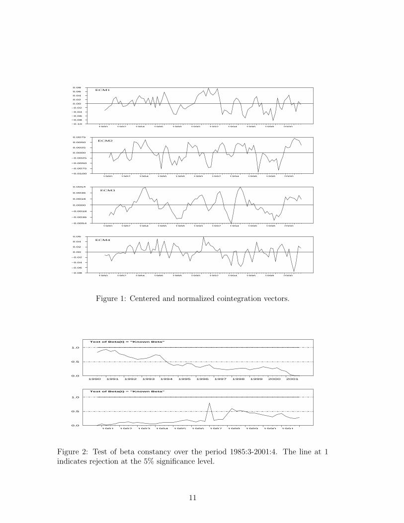
Finally, the hypothesis that the relations tested in the first four hypothesesjointly span the cointegration space cannot be rejected (p-value 0.09). The re-stricted estimates of the cointegration vectors are reported in table 3 and figure1 shows the centered and normalized linear combinations of the variables, β′1Xt,β′2Xt, β

′3Xt and β′4Xt labeled as ecm1, ecm2, ecm3 and ecm4 respectively. Note

that the vectors in table 3 span an identified system. The identified cointegrationspace was also tested for parameter constancy by a recursive test described inHansen and Johansen (1993). The results are reported in figure 2 where the recur-sions have been performed both forwards and backwards to cover the completeperiod. The tests indicate that the parameters of the identified cointegrationspace have been constant for the time period of the analysis13.

12Arrow et al. (1961) show that b in the regression qt = a + bwt + εt provides an estimate ofthe elasticity of substitution when labor and product markets are competitive. Taking the timeseries properties of the data into account, this would correspond to testing the stationarity ofthe relation in H4.

13The same is not true for the short-run parameters which have fluctuated in particularduring the late 80’s and the beginning of the 90’s when Finland experienced a strong boomfollowed by a deep recession. Thus, more care should be taken when interpreting the short-runeffects.

10

1980 1982 1984 1986 1988 1990 1992 1994 1996 1998 2000−0.10

−0.08

−0.06

−0.04

−0.02

0.00

0.02

0.04

0.06

0.08ECM1

1980 1982 1984 1986 1988 1990 1992 1994 1996 1998 2000−0.0100

−0.0075

−0.0050

−0.0025

0.0000

0.0025

0.0050

0.0075

ECM2

1980 1982 1984 1986 1988 1990 1992 1994 1996 1998 2000−0.0054

−0.0036

−0.0018

0.0000

0.0018

0.0036

0.0054

ECM3

1980 1982 1984 1986 1988 1990 1992 1994 1996 1998 2000−0.08

−0.06

−0.04

−0.02

0.00

0.02

0.04

0.06

ECM4

Figure 1: Centered and normalized cointegration vectors.

1990 1991 1992 1993 1994 1995 1996 1997 1998 1999 2000 20010.0

0.5

1.0

Test of Beta(t) = "Known Beta"

1981 1982 1983 1984 1985 1986 1987 1988 1989 1990 19910.0

0.5

1.0

Test of Beta(t) = "Known Beta"

Figure 2: Test of beta constancy over the period 1985:3-2001:4. The line at 1indicates rejection at the 5% significance level.

11

Table 3: Identified β-vectors (t-vales in brackets).

β1 β2 β3 β4

w 1 0 0 0

u 0 1 0 0

y 0 0.05 0 -0.81(12.69) (-18.32)

l 0.13 0 0 1(2.21)

r 6.72 0.84 1 0(4.83) (7.83)

∆p 0 0.74 0 0(12.28)

c -0.13 0 -0.05 0(-2.21) (-9.80)

t -0.01 0 0.001 0.01(-10.87) (15.95) (23.21)

4.2 The short-run structure of the model

The short run structure of the model was estimated by taking the long-run rela-tions as given from the previous section. The short-run structure was modeledby

∆X1,t = Γ1∆X2,t + Γ2∆Xt−1 + αECMt−1 + µ+ ΨDt + εt (11)

where X1,t contains the endogenous variables and X2,t the exogenous variable,Γ1 is a (6 × 1) matrix, Γ2 is a (6 × 7) matrix and α is a (6 × 4) matrix, ECMt

is a column vector with ecmi,t as elements and Dt includes sesonals and an un-restricted constant. Initial testing of zero restrictions on the parameters of thecomplete system by F-tests indicated that ∆wt−1, ∆ut−1, ∆yt and ∆lt could beexcluded (p-values 0.14, 0.32, 0.31 and 0.48 respectively). The system was thenre-estimated with these changes. The results from misspecification tests on theestimated residuals from the equations are reported in table 4 (the numbers arep-values). By and large, the model seems to fit the data quite well, although nor-mality is rejected in the unemployment equation. This is due to a large outlier inthe first quarter of 1987. However, modeling this outlier does not alter the resultssignificantly. There might also be a small problem with ARCH in the interestrate equation (the null of no ARCH is rejected at the 5% significance level butnot at the 1% level).

The result from imposing zero restrictions on the individual equations are

12

Table 4: Misspecification tests on the estimated residuals from each equation.The tests are described in Doornik and Hendry (2001). The normality test isderived under the null of normality. The null in the ARCH test is no conditionalheteroscedasticity and the null in the AR 1-5 test is no autocorrelation in thefirst 5 lags. Bold values indicate rejection at 5% significance.

Equ. “normality χ2” ARCH AR 1-5 correlation(obs/est)

∆w 0.20 0.79 0.10 0.76∆u 0.001 0.86 0.87 0.81∆y 0.23 0.24 0.10 0.96∆l 0.90 0.95 0.09 0.97∆r 0.49 0.02 0.38 0.70∆2p 0.08 0.83 0.76 0.84

reported in table 5. As noted in section 2, our primary interest is in the equationsdetermining the change in the real wages and the change in the unemploymentrate (equations 1 and 2 in table 5). Writing out these equations explicitly wehave

∆wt = −0.27(w + 6.72r − 0.13k)t−1 + 0.22(l − 0.81y + 0.01t)t−1 (12)

and

∆ut = −0.2∆ct − 0.31∆rt−1 + 0.09∆2pt−1 + 0.48(r − 0.05c+ 0.01t)t−1

−0.29(u+ 0.05y + 0.84r + 0.74∆p)t−1 (13)

where ecm1 and ecm4 in (12) and ecm2 and ecm3 in (13) are written out in full.

5 Interpretation of the results

5.1 The elasticity of substitution

Equation (12) describes the change in real manufacturing wages due to imbalancesin the long-run relationships ecm1 and ecm4. Note that only ecm1 is errorcorrecting in the wage equation (since wt does not appear in ecm4), so that theother variables, kt and rt, are determining the change in wages in that relation.Since the capital-labor share enter in ecm1, the long-run relationship between thereal wages and the capital-labor share is empirically established. This relationshipis consistent with σ 6= 1 in (3) and therefore inconsistent with the standard Cobb-Douglas production function. Furthermore, the coefficients in equation (12) implythat this relationship is positive. To see this consider a small positive increase

13

Table 5: The short-run structure of the model. Coefficients in boldface indicatesignificance at the 5% level of the deterministic components (lowest part of thetable).

Equ1 Equ2 Equ3 Equ4 Equ5 Equ6∆wt ∆ut ∆yt ∆lt ∆rt ∆2pt

∆ct – -0.20 4.71 2.25 – -0.39(-4.26) (4.18) (3.12) (-3.46)

∆ct−1 – – -6.74 – – –– (-6.27)

∆rt−1 – -0.31 – – -0.58 0.96(-2.29) (-6.58) (2.99)

∆2pt−1 – 0.09 – 1.35 – –(2.37) (2.33)

ecm1t−1 -0.27 – -0.33 – –(-4.34) (-4.40)

ecm2t−1 – -0.29 – -2.04 – -0.86(-5.55) (-3.01) (-7.08)

ecm3t−1 – 0.48 – – -0.26 0.54(5.25) (-5.20) (-2.48)

ecm4t−1 0.22 – 0.29 -0.78 -0.06(3.41) (3.00) (-8.33) (-4.87)

Constant 0.01 0.00 0.02 -0.01 -0.00 0.00Seasont 0.03 -0.00 -0.12 -0.11 -0.00 0.01Seasont−1 0.01 0.00 -0.08 -0.06 0.00 0.01Seasont−2 -0.01 0.00 -0.21 -0.21 0.00 0.00

14

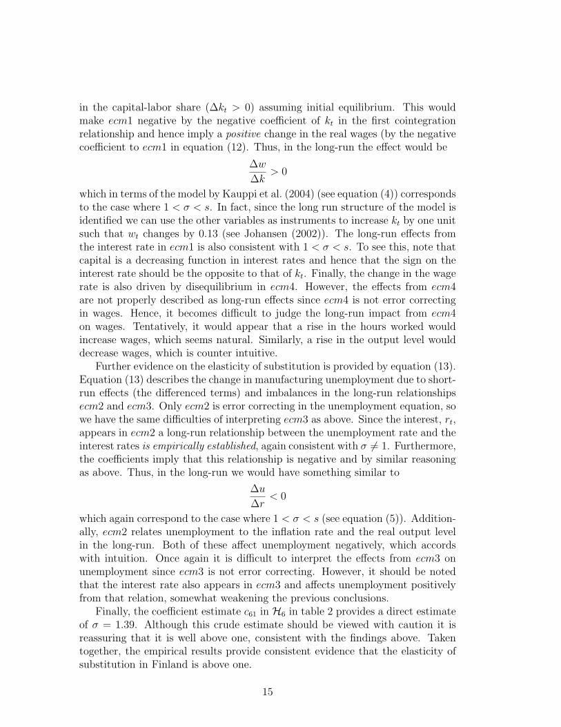
in the capital-labor share (∆kt > 0) assuming initial equilibrium. This wouldmake ecm1 negative by the negative coefficient of kt in the first cointegrationrelationship and hence imply a positive change in the real wages (by the negativecoefficient to ecm1 in equation (12). Thus, in the long-run the effect would be

∆w

∆k> 0

which in terms of the model by Kauppi et al. (2004) (see equation (4)) correspondsto the case where 1 < σ < s. In fact, since the long run structure of the model isidentified we can use the other variables as instruments to increase kt by one unitsuch that wt changes by 0.13 (see Johansen (2002)). The long-run effects fromthe interest rate in ecm1 is also consistent with 1 < σ < s. To see this, note thatcapital is a decreasing function in interest rates and hence that the sign on theinterest rate should be the opposite to that of kt. Finally, the change in the wagerate is also driven by disequilibrium in ecm4. However, the effects from ecm4are not properly described as long-run effects since ecm4 is not error correctingin wages. Hence, it becomes difficult to judge the long-run impact from ecm4on wages. Tentatively, it would appear that a rise in the hours worked wouldincrease wages, which seems natural. Similarly, a rise in the output level woulddecrease wages, which is counter intuitive.

Further evidence on the elasticity of substitution is provided by equation (13).Equation (13) describes the change in manufacturing unemployment due to short-run effects (the differenced terms) and imbalances in the long-run relationshipsecm2 and ecm3. Only ecm2 is error correcting in the unemployment equation, sowe have the same difficulties of interpreting ecm3 as above. Since the interest, rt,appears in ecm2 a long-run relationship between the unemployment rate and theinterest rates is empirically established, again consistent with σ 6= 1. Furthermore,the coefficients imply that this relationship is negative and by similar reasoningas above. Thus, in the long-run we would have something similar to

∆u

∆r< 0

which again correspond to the case where 1 < σ < s (see equation (5)). Addition-ally, ecm2 relates unemployment to the inflation rate and the real output levelin the long-run. Both of these affect unemployment negatively, which accordswith intuition. Once again it is difficult to interpret the effects from ecm3 onunemployment since ecm3 is not error correcting. However, it should be notedthat the interest rate also appears in ecm3 and affects unemployment positivelyfrom that relation, somewhat weakening the previous conclusions.

Finally, the coefficient estimate c61 in H6 in table 2 provides a direct estimateof σ = 1.39. Although this crude estimate should be viewed with caution it isreassuring that it is well above one, consistent with the findings above. Takentogether, the empirical results provide consistent evidence that the elasticity ofsubstitution in Finland is above one.

15

5.2 A brief discussion of the remaining equations of themodel

The remaining equations in table 5 are briefly discussed in this section. The focuswill be on the empirical consistency of the long-run effects in each of the remainingequations, i.e. on the error correcting equilibrium relations. Equation 3 explainsthe changes in manufacturing output where only ecm4 is error correcting. Theinterpretation from this equilibrium relationship is straightforward. An increasein the hours worked in manufacturing leads to a long-run increase in output(however, output increases slightly less than the initial increase in hours worked).Additional effects on the change in output stem from ecm1 and the short-runeffects.

Equation 4 explains the changes in hours worked in manufacturing. As withoutput, only ecm4 is error correcting in that equation and the effects are similar,i.e. increased output leads to more hours worked. Thus, there exists a two wayrelationship between the hours worked and the output. In addition, the hoursworked are affected by disequilibrium in ecm2 and other short-run effects.

Equation 5 explains the change in the long-term interest rate where onlyecm3 is error correcting. The effects from increased real capital is higher interestrates, which is somewhat counterintuitive. However, note that since capital isexogenous in the time frame of this analysis, this might a consequence of excesscapital demand on the interest rates in the medium term. Intuitively, when thereis a high demand for capital, interest rates start to increase.

Finally, equation 6 describes the change in inflation where only ecm2 is er-ror correcting. An increase in unemployment decreases inflation, which seemsnatural. However, increases in output or the interest rates appears to decreaseinflation, which is counter intuitive. In addition the change in inflation is alsoaffected by disequilibrium in ecm3 and ecm4 and by other short-run effects.

6 Conclusions

In this paper, an indirect method for making econometric inference on the pa-rameter region of the elasticity of substitution, utilizing functional relationshipsthat depend on this elasticity, was proposed. Compared with alternative meth-ods of estimating the elasticity, the present approach provides enough flexibilityto allow for more data oriented modeling while still retaining a firm connectionto economic theory. A positive long-run relationship between real manufacturingwages and the capital-labor share and a negative long-run relationship betweenthe unemployment rate and the interest rate were established by estimating acointegrated VAR-model on Finnish manufacturing data. These relationshipshave implications for the parameter region of the elasticity of substitution asdemonstrated in Kauppi et al. (2004). In particular, the results are consistent

16

with a modeling approach for the Finnish economy that uses a CES productiontechnology with an elasticity of substitution above one coupled with imperfec-tions in both product and labor markets. A rough estimate of the elasticity ofsubstitution equal to 1.39 was also obtained.

References

Antras, P., 2004. Is the U.S. Aggregate Production Function Cobb-Douglas? NewEstimates of the Elasticity of Substitution. Contributions to Macroeconomics4 (1).

Arrow, K., Chenery, H., Minhas, B., Solow, R., 1961. Capital-Labor Substitutionand Economic Efficiency. Review of Economics and Statistics 43, 225–250.

Azariadis, C., 1996. The Economics of Powerty Traps Part One: Complete mar-kets. Journal of Economic Growth (1), 449–486.

Bentolila, S., Saint-Paul, G., 2003. Explaining Movements in the Labor Share.Contributions to Macroeconomics 3 (1).

Berndt, E., 1976. Reconciling Altenative Estimates of the Elasticity of Substitu-tion. Review of Economics and Statistics 58 (1), 81–114.

Blanchard, O., Giavazzi, F., 2003. Macroeconomic Effects of Regulation andDeregulation in Goods and Labor Markets. Quarterly Journal of Economics, 879–907.

Chirinko, R., Fazzari, S., Meyer, A., 2004. That Elusive Elasticity: A Long-Panel Approach to Estimating the Capital-Labor Substitution Elasticity. CE-Sifo working paper 1240.

Dixit, A., Stiglitz, J., 1977. Monopolistic Competition and Optimum ProductDiversity. American Economic Review 67 (3), 297–308.

Doornik, J., Hendry, D., 2001. Empirical Econometric Modelling Using PcGive.London: Timberlake Consultants Press.

Duffy, J., Papageorgiou, C., Mar. 2000. A Cross-Country Empirical Investiga-tion of the Aggregate Production Function Specification. Journal of EconomicGrowth 5, 87–120.

Engle, R., Granger, C., Mar. 1987. Co-integration and Error Correction: Repre-sentation, Estimation and Testing. Econometrica 55 (2), 251–76.

Felipe, J., Fisher, F., May 2003. Aggregation in Production Functions: WhatApplied Economists should Know. Metroeconomica 54 (2), 208–263.

17

Hansen, H., Johansen, S., 1993. Recursive Estimation in Cointegrated VAR-models. Preprint 1993, No. 1, Institute of Mathematical Statistics, Universityof Copenhagen .

Hendry, D., Juselius, K., 1999. Explaining Cointegration Analysis: Part I. EnergyJournal 21 (1), 1–42.

Hendry, D., Juselius, K., 2000. Explaining Cointegration Analysis: Part II. En-ergy Journal forthcoming.

Johansen, S., 1995. Likelihood-based Inference in Cointegrated Vector Autore-gressive Models. Oxford University Press.

Johansen, S., 2002. The Interpretation of Cointegrating Coefficients in the Coin-tegrated Vector Autoregressive Model. Preprint .

Johansen, S., Juselius, K., 1990. Maximum Likelihood Estimation and Inferenceon Cointegration – With Applications to the Demand for Money. Oxford Bul-letin of Economics and Statistics 52 (2), 169–211.

Jones, L., Manuelli, R., 1990. A Convex Model of Equilibrium Growth: Theoryand Policy Implications. Journal of Political Economy 98.

Kauppi, H., Koskela, E., Stenbacka, R., Oct. 2004. Equilibrium Unemploy-ment and Capital Intensity Under Product and Labour Market Imperfections.Helsinki Center of Economic Research, Discussion Paper 24.

Klump, R., McAdam, P., Willman, A., Jun. 2004. Factor Substitution and FactorAugmenting Technical Progress in the US: A Normalized Supply-Side SystemApproach. ECB Working Paper Series 367.

Mairesse, J., Hall, B., Mulkay, B., 1999. Firm-Level investment in France and theUnited States: An Exploration of What We Have Learned in Twenty Years.Annales d’Economie et de Statistique (55-56), 27–67.

Nickell, S., 1997. Unemployment and Labor Market Rigidities: Europe versusNorth America. Journal of Economic Perspectives 11 (3), 55–74.

Quah, D., Jun. 1996. Empirics for Economic Growth and Convergence. EuropeanEconomic Review 40 (6), 1353–76.

Ripatti, A., Vilmunen, J., 2001. Declining Labour Share - Evidence of a Changein the Underlying Production Technology? Bank of Finland Discussion Papers(10).

Solow, R., Feb. 1956. A Contribution to the Theory of Economic Growth. Quar-terly Journal of Economics 70, 65–94.

18

Solow, R., 1994. Perspectives on Growth Theory. Journal of Economic Perspec-tives 8 (1), 45–54.

Spector, D., Feb. 2004. Competition and the Capital-Labor Conflict. EuropeanEconomic Review 48, 25–38.

19