The relationship between capital flows and current account:

volatility and causality

Selen Sarisoy Guerin∗

ECARES, Université Libre de Bruxelles

Abstract

This paper examines the relationship between net private capital inflows and the

current account in a set of industrial and developing countries. The first question asks

whether the cyclical volatility in current accounts can be explained by the volatility of

capital flows. The second question addresses the causal link between net capital

inflows and current account imbalances. There is evidence in our data that inflows do

cause current account imbalances in the developing countries. In contrast, the

evidence implies that inflows do not cause current account imbalances in the

industrial countries, nor does the inflow volatility affect current account volatility.

JEL classification: F32; F21

Keywords: Capital flows; Current Account; Unit root tests; Engle-Granger causality;

ECM

∗ Corresponding author. Tel.: +32 2650 4602 E-mail address: sguerin@ulb.ac.be

1

1. Introduction

This paper examines the relationship between net private capital inflows and

the current account in a set of industrial and developing countries. International

capital flows among industrial countries soared in the 1980s, and the flows from

industrial to developing countries resumed their pre-debt crisis levels in the 1990s.

This surge in international capital flows to developing countries coincided with

widening current account deficits in many of these countries. Running large current

account deficits also became common among industrial countries. Australia, New

Zealand, Portugal and the US have been running large current account deficits for the

most part of the 1990s. At the end of 2000, the US current account deficit reached to

$415.5 billion, equivalent to 4.5 percent of US GDP (IMF, 2001). The empirical

evidence suggests that inflows are increasingly used to finance current account

deficits in some developing countries, and reversals in current accounts are often

accompanied by reversals in international capital inflows1.

Theoretical models of capital flows and empirical evidence suggest that while

foreign capital can stimulate growth, smooth consumption, provide portfolio

diversification and productive efficiency, they also incur some costs2. Free flow of

capital possibly comes at the cost of increased contagion, monetary instability and a

1 Milesi-Ferretti and Razin (1996, 1998, 1999) study the probability of a crisis in the face of current account reversals, which are often associated with reversals in capital flows. 2 The theoretical benefits from capital flows were based on a benchmark of perfect capital mobility as was assumed in neoclassical trade and economic growth theories.

2

loss of independence on domestic policies3. Calvo et al. (1996) argue that widening

current account deficits is one of the less desirable macroeconomic effects of large

capital inflows to the debtor countries. In the first half of the 1990s, larger shares of

capital inflows were allocated to reserve accumulation in developing countries4.

Recent trends indicate that reserve accumulation is slowing as an increasing

proportion of capital flows is financing current account deficits (IMF, 2001).

Current account imbalances are not strictly a phenomenon of the 1990s.

Following the oil price shocks in the 1970s, there have been large swings in the

current account balances of most countries. Persistent current account deficits raised

concern over their sustainability. The empirical evidence suggested that while some

countries such as Ireland, Australia, Israel, Malaysia and South Korea were able to

sustain large current account deficits for many years, other countries such as Chile

and Mexico suffered severe losses5. Excessive current account deficits in crisis

countries were also a prevalent feature of the 1997 Asian crisis.

Large private capital inflows may affect the behaviour of the current account

through their effect on savings and investment. Current account imbalances are

caused by a mismatch between savings and investment. Periods of large capital

inflows are generally accompanied by increased rates of investment. If international

capital inflows are used to increase investment, assuming savings remain stable, this

may imply an increase in the current account deficit. When capital flows are reversed,

3 See, for example, Calvo et al. (1996), and Goldstein et al. (1994) for a discussion on trends in capital flows in 1990s and costs and benefits from them. 4 From 1990 to 1994, the share of capital flows that were accumulated in reserves was 59 percent in Asia and 35 percent in Latin America (Calvo et al. 1996). 5 See Milesi-Ferretti and Razin (1996).

3

there may be sharp reductions (or reversals) in the current account, as well as

macroeconomic costs6.

The first question addressed in this paper is whether cyclical volatility in net

inflows has any effect on current account volatility. Using panel fixed-effect

regression analysis, the volatility of the capital flows and the current account in a set

of industrial and developing countries are examined. The second question addressed is

whether capital flows cause current account imbalances. As a first step, cointegration

techniques are used to establish whether capital inflows and current account

imbalances are related. The direction of causality is then tested by standard Granger

causality tests and causality tests on ECM (error correction model). Finally,

cointegrating regressions are estimated between the current account imbalances and

net inflows.

The remainder of this paper is organized as follows. Section 2 provides the

theoretical and empirical background for the relationship between capital flows and

the current account. Section 3 examines the (unconditional) volatility of the current

account and the components of the capital account for individual countries. Section 4

presents the results of the panel fixed-effects data estimation. Section 5 addresses the

question whether capital flows cause current account imbalances by using

cointegration and causality tests, and estimates cointegrating regressions for the

countries where the causality runs from inflows to the current account. Section 6

concludes.

6 See Hutchison and Noy (2002) for output costs of sudden-stop crises, and see IMF (1999), Claessens et al.( 1995); Sarno and Taylor (1997); Bacchetta and Wincoop (1998) for volatility in capital flows.

4

2. Theoretical and Empirical Background

In a closed economy, the current account balance is zero, as savings must

equal investment. In open economies, however, domestic agents can borrow or lend in

international capital markets in the face of shocks to income and smooth consumption.

Savings can be allocated to accumulating domestic assets or foreign assets, and

investment can be financed by accumulating domestic assets or by issuing foreign

liabilities. The resultant current account deficit is the outcome of an intertemporal

decision of consumption and saving in an open economy with capital mobility, in the

tradition of Irving Fisher (Calvo et al. 1996).

Calvo et al. (1996) argue that the effect of capital inflows on the current

account can be derived from standard open economy models, such as Irving Fisher’s

model. In such a model, a fall in interest rate will induce income and substitution

effects, for debtor countries, which results in a consumption boom and a widening in

the current account deficit. For capital-importing countries, a decline in interest rates

reduces the present value of its debt and also makes further borrowing cheaper. Thus,

standard open economy models suggest that increased capital inflows are likely to be

accompanied by a rise in consumption and investment, and a widening in the current

account7. This effect of capital inflows is similar to the effect of a decrease in interest

rates.

These models imply that investment and saving, and ultimately the current

account balance, may depend on capital flows. It is also likely that the capital inflows

a country receives are endogenously determined by its macroeconomic fundamentals.

There are some studies such as the well-known study by Feldstein and Horioka (1980)

7 Calvo and Vegh (1993) offer an alternative approach with a focus on monetary economy with similar implications.

5

that derive conclusions on international capital mobility from theories on the current

account. Since widening current account deficits were usually accompanied with

increased investment and a fall the in rate of savings, this was accepted as a sign of

the high integration of capital markets. Feldstein and Horioka (1980) interpreted the

slope coefficient of a regression of investment on savings as a measure of

international capital mobility. The high correlation between investment and saving led

them to argue that there is less than perfect capital mobility.

The relationship between capital inflows and current account dynamics is

formalized by the consumption-smoothing theory. The consumption-smoothing

approach combines the assumptions of high capital mobility and permanent income

theory of consumption in a small, open economy to predict what capital flows would

be if agents behave in accordance with the permanent income theory. According to

this approach, a country’s current account will be in deficit whenever national cash

flow (i.e. GDP less investment less government spending), is expected to rise over

time. It will be in surplus whenever national cash flow is expected to fall. Ghosh and

Ostry (1995) argue that the intertemporal model of the current account therefore

provides a benchmark for judging what capital flows should be, given specific shocks

affecting economy.

In an empirical study, Ghosh and Ostry (1993) use the consumption-

smoothing model as a benchmark for calculating optimal capital flows, i.e. flows that

can smooth consumption in the face of shocks to the national cash flow. They

compare the actual series to the benchmark series and conclude that flows to the

developing countries were determined by economic fundamentals to a significant

degree. Ghosh and Ostry (1995), in another paper, calculate optimal current account

levels for a sample of forty-five developing countries, using a vector autoregression

6

analysis, and conclude that actual current account levels suggest consumption

smoothing, or high capital mobility.

Other empirical studies on the determinants of current account, such as

Calderon et al. (2002), Chinn and Prasad (2000), and Freund (2000) find that net

foreign assets have significant power in explaining the CA/GDP ratios in developing

and industrialized countries. Recent studies by Kraay and Ventura (2000, 2002)

introduce a new rule to assess the response of the current accounts in debtor and

creditor countries following a temporary income shock. The current account response,

they propose, equals the savings generated by the shock multiplied by the country’s

share of foreign assets in total assets. One important implication of this study is that

this new rule implies that favourable shocks lead to deficits in debtor countries and

surpluses in creditor countries. In the long-run, they find that countries invest a

marginal unit of wealth in domestic and foreign assets in the same proportion as their

initial portfolio, which implies that country portfolios are remarkably stable. In the

short-run, a marginal unit of saving is mostly invested in foreign assets.

A study by Bosworth and Collins (1999) examines the relationship between

capital flows to developing countries and the current account. They use a panel data

set that includes 58 developing countries over 17 years (1979-1995) to analyse the

effect of capital flows on investment and savings and the current account. They

conclude that a large proportion of capital flows to the developing countries over the

past two decades have been used to finance current account deficits. These resource

transfers were primarily used to finance investment, not to increase consumption.

When they examine different types of capital flows, they find that FDI has highly

beneficial effects on investment, whereas portfolio flows have no impact.

7

Lane and Milesi-Ferretti (2001) examine how net foreign asset positions affect

the behaviour of the trade balance. This relationship is tested in a panel data set that

includes 20 industrial and 38 developing countries for the sample period 1970-1998.

Their results from panel fixed-effect regressions conclude that there is a statistically

significant relationship between the (transfer adjusted) trade balance and the dynamics

of the net foreign assets position in both industrial and developing countries. Holding

fixed the fundamentals and short-run fluctuations from the long-run equilibrium, the

trade balance is negatively correlated to returns on the outstanding net foreign asset

position. This relationship is found to be stronger in developing countries than it is in

industrial countries.

Above, a number of papers that examine the relationship between current

account and capital flows are summarized. These theoretical and empirical studies

provide a rich background on which this paper aims to build on. The contribution of

this paper to the existent literature is in examining causal links between the volatility

of capital flows and the current account. The study by Fry et al. (1995), which

examines Granger causality between capital account and current account imbalances,

is the closest study to this chapter. They focus on FDI flows to 46 developing

countries and test whether such flows are autonomous or accommodating vis-à-vis the

current account and other capital flows. This paper extends on their study by

including industrial countries as well as a set of developing countries in the sample

and the data period covers the surge in international capital flows of the1990s. This

paper also differs from the study of Fry et al. (1995) since it combines the volatility of

capital flows with causality between capital flows and the current account.

8

3. Volatility

Recent trends of international capital flows to the developing countries

indicate that large capital flows that were directed to emerging markets were easily

reversible, suggesting that these flows were highly volatile. Sharp capital outflows

from and/or sudden cessation of foreign capital inflows (i.e. sudden stops) to

emerging markets have been commonly observed characteristics of several recent

financial crises. Such extreme volatility is often associated with severe consequences

for the economy. For example, a sudden reversal of foreign capital inflows may cause

a sharp drop in domestic investment, domestic production and employment

(Hutchinson and Noy, 2002)8. Besides the loss of output caused by sudden stops of

international capital flows, volatility of international capital flows creates instability

by introducing uncertainty to the economy. For this reason, economists concentrated

on the factors that may contribute to volatility in international capital flows.

One particular focus was based on analysing characteristics of different types

of capital flows. This approach was partly justified by the emergence of a new

combination of international capital flows that dominated the 1990s compared to the

1980s. First, the majority of capital flows in the 1990s to the developing countries

were private flows, contrary to the official flows of the 1980s. Second, portfolio

equity and foreign direct investment flows constituted the majority of private capital

flows to emerging markets, which were facilitated by the liberalization of emerging

market economies and technological developments. The increased reliance on

portfolio equity capital for foreign finance in these markets and the short-term nature

8 Recent theoretical literature emhpasizes the linkages between sudden stops and output losses (e.g. Aghion et al., 2001; Mendoza, 2001).

9

of these flows, compared to long-term commitment characteristic of direct

investment, also justified concerns on increased volatility.

The experience of the 1997 Asian crisis indicated that portfolio equity capital

flows have been highly volatile and have turned negative, while foreign direct

investment has remained stable (World Bank, 1999). Analysis of the volatility of

international capital flows in some studies (e.g. Turner, 1991) was based on Meade’s

distinction between ‘temporary’ and ‘continuing’ capital movements. Meade (1951)

described ‘temporary’ flows as short-term funds attracted by interest rate differentials.

This definition implied that capital pulled in by certain temporary factors was

reversible once the attraction disappeared. Turner (1991) found that for the period

1975-82, the elements of the capital account with greatest volatility were public sector

and short-term banking flows, in a sample of five industrial countries9. For the period

1983-89, Turner found that the volatility of bonds and equity investment was much

higher. In terms of hierarchy of volatility, direct investment flows have been among

the least volatile, whereas portfolio equity flows have been particularly volatile.

Osei et al. (2002) study the volatility of capital flows to a sample of 60

developing countries over the period 1970 to 1997. Their results indicate that

volatility has increased in the 1990s, relative to the 1980s, but not to the 1970s. A

study on the volatility of portfolio capital flows by Claessens et al. (1995) focus on

the speculative and unstable behaviour of portfolio capital flows, compared to direct

investment. Using time-series analysis, their results, perhaps surprisingly, indicate that

one cannot tell the difference between long-term and short-term flows in terms of

volatility. In a sample of ten industrial and developing countries, they find that long-

term flows are as volatile as short-term flows. Sarno and Taylor (1997) also analyse

9 The sample included the US, Japan, Germany, Canada and the UK.

10

the persistence of portfolio flows to a group of Latin American and Asian developing

countries. They conclude that portfolio flows to these countries over the sample

period (1988-92) may be regarded as entirely temporary.

These studies highlight the importance of the volatility of international capital

flows and its policy implications. The focus of this paper, however, is not based on

identifying the volatility of different types of capital flows. The issue that we seek to

address is the relationship between volatility of the current account and the volatility

of the capital account. It is often mentioned in the literature that one important feature

of the recent trends in capital flows to developing countries is that private equity and

bond flows as opposed to official capital flows are increasingly a crucial source of

large current account imbalances (e.g. Sarno and Taylor, 1997). This may have policy

implications in terms of the sustainability of recent current account deficits.

In this section, the balance-of-payments identity is used to analyse current and

capital account volatility. The balance-of-payments accounting relates current

account transactions to capital account transactions. Hence, any international

transaction requires two offsetting entries to the balance of payments: One entry on

the current account and the other entry on the capital account. In theory, the current

account and capital account should add up to zero, but almost always a discrepancy

item, called errors and omissions, is required as described below:

Balance of Payments = Current Account + Capital Account = 0, (1)

or

0 = Current Account + Inflows + Outflows + ∆Reserves + Errors10 (2)

10 We have included the capital account (a new item that records capital transfers and transactions related to the purchase and sale of used equipment) in the errors and omissions item.

11

The equation (2) is based on the balance of payments identity in the fifth

edition of IMF’s Balance of Payments Manual. By convention, the sources of foreign

exchange, such as exports and inflows are denoted as positive, and uses of foreign

exchange, such as imports and outflows, are denoted as negative. This identity

requires that a current account transaction can be offset by a capital account

transaction, via any of the components. Inflows do not always finance current account

deficits. They can be used to increase outflows and to build reserve assets. This

suggests that the volatility in international capital inflows need not always be

transferred one-for-one to the current account, if the inflows are channelled into

outflows or reserves11.

As a first step, we examine the unconditional volatility in the current account

and components of capital account. From equation (2), the variance of the current

account (CA) can be shown to be equal to the variance of the capital account (KA),

and its components:

var (CA) = var (KA) (3)

var(CA) = var (In) + var (Out) + var (∆Res) + var(Err)+ 2covar(In,Out)

+2covar(In, ∆Res) +2covar(In,Err) +2covar(Out, ∆Res)

+2covar(Out, Err) + 2covar(∆Res, Err) (4)

11 We refer to private outflows by the use of the word ‘outflows’. Reserve account, which can be categorized as public outflows is treated separately.

12

Equation (4) implies that the individual components of the capital account can

be more or less volatile than the current account. For example, capital inflows and

outflows can be highly volatile, as suggested by the empirical literature12. However, if

gross inflows are negatively correlated with gross outflows, the impact of net inflows

on the current account may be stabilizing. Conversely, net inflows can add to the

volatility in the current account, if net inflows are positively correlated with official

reserves13.

Tables 1a and 1b present results of the volatility analysis of the current

account and the components of the capital account for a set of industrial countries and

developing countries (See Appendix for the list of countries). The sample was

determined by data availability. The data for industrial countries cover all major

financial investors with the exception of Ireland and Greece. In terms of the data on

developing countries, the set of developing countries includes the major recipients of

international capital flows. The sample period differs for each country. The annual

data on the balance-of-payments statistics are taken from IMF’s International

Financial Statistics (2001) database. The current account and the components of the

capital account are all expressed as a percent of the GDP. The volatility of each series

is calculated as the standard deviations of the ratios. All variables are in 1996 constant

US$, deflated by the US GDP deflator. Both Tables 1a and 1b report results from HP

(100) filtered series that enable us to concentrate on the cyclical component of the

12 See Turner (1991) for an account of the volatility of different capital flows in the 1980s, and IMF (1999) for the volatility in capital flows in the 1990s. 13 The errors and omissions is an equilibrating item in the capital account, therefore it is endogenously determined.

13

series14. We chose to report results only from HP (100) series since this method helps

us concentrate on the cyclical volatility without loss of degrees of freedom and

valuable information on the long-run trends15.

There are clear differences between industrial and developing countries in our

sample. For the industrial countries, inflows and outflows are more volatile than the

current account, whereas for the developing countries outflows are more stable than

both inflows and the current account. This may suggest that inflows are mostly offset

by outflows in industrial countries. Although many developing countries started

liberalizing their capital accounts, restrictions such as capital controls imply that these

countries do not have fully open financial markets16. Even for industrial countries,

capital account liberalization came as late as the 1980s, where barriers were lowered

and controls were abolished. By the late 1980s, there were only six industrial

countries in the world with fully open financial markets: Canada, Germany,

Netherlands, Switzerland, UK and US.

The relatively high volatility of reserves in the developing countries, compared

to the industrial countries is another difference. During a surge period of capital

inflows, policymakers in emerging markets often intervened to limit the expansionary

consequences of capital inflows. Often, sterilization of capital inflows was the policy

tool used. This involved a swap of international reserves for public bonds or increased

reserve requirements. During the early 1990s in Chile, sterilization meant that over

14 Hodrick-Prescott filter is used in empirical studies to identify the business-cycle component of the macroeconomic time-series. HP filter minimizes the variance of the cyclical component subject to a penalty for the variation in the second difference of the growth component, where a smoothness parameter penalizes the variability in the growth component. Recently, the use of HP filter and the somewhat arbitrary choice of the smoothness parameter has been criticized (King and Rebelo, 1993; Harvey and Jaeger (1993); Baxter and King (1995); Guay and St-Amant (1997)). 15 Another alternative is first-differencing the series. The results are qualitatively similar to the results of HP (100) filtered series. 16 Johnston and Tamirisa (1998) show that controls on capital outflows are more prevalent than controls on inflows on all types of transactions, except in the case of FDI and real estate purchase.

14

three quarters of capital inflows (7 percent of GDP) went to international reserves

accumulation in the central bank every year (Caballero and Krishnamurthy, 2001).

Bosworth and Collins (1999) also show that for developing

countries, around one-third of capital inflows were channelled into reserves.

Aizenman and Marion (2002) argue that, following a crisis, countries that have

increased perceived sovereign risk will increase their demand for international

reserves, as was the case for East Asia after 199717. Today developing countries hold

60.4 percent of total global reserves.

4 Panel Data Analysis

In this section, the relationship between the current account and net capital

inflow volatility is examined in a panel fixed-effects regression framework. Panel data

analysis concentrates on the effect of (conditional) volatility of capital inflows on the

current account in industrial countries versus in developing countries. As the

examination of unconditional volatility for individual industrial and developing

countries suggests, these two country groups exhibit different dynamics in their

current and capital accounts. Pooling cross-country and time-series data often

produces more efficient results than examining time-series or cross-country alone

(Verbeek, 1999). While a panel fixed-effects estimator concentrates on within

variation (i.e. the dynamic response of the current account to net inflows volatility),

the country fixed-effects controls for unobserved heterogeneity. The previous section

suggests considerable cross-country heterogeneity in the current account and capital

17 Lane and Burke (2001) find that trade openness is by far the most important determinant of reserve holdings in cross-country sample of industrial and developing countries. Trade openness can proxy for vulnerability to external shocks.

15

account dynamics of both industrial and developing countries. In such a case, fixed-

effects panel regression should produce more efficient results compared to pooled

OLS estimation18.

4.1 Model

The volatility of current account is formulated as a function of the volatility of

net private inflows as follows:

V(CAit) = αi + β1 (V(Inflowi,t ))+ tt + εi t (5)

where:

V(CAit): volatility of CA to GDP ratio of country i at time t,

V(Inflowit): volatility of inflows to GDP ratio of country i at time t,

tt: year dummies.

The sample periods for annual data on current account and capital flows vary

for each country19. The volatility of the current account and capital inflows, measured

as standard deviations of respective variables, were calculated over 5-year non-

overlapping periods for the sample period 1970-200020. Both current account and net

inflows have been normalized by country size (i.e. dividing the respective variables

by the GDP of the country). Here we measure volatility of inflows and the current

18 Pooled OLS estimation models do not control for individual heterogeneity, therefore, run the risk of obtaining biased results (Baltagi, 1999). 19 We choose to use annual data instead of quarterly data since this allows us to work with a larger sample. 20 The last period includes 6 years and runs from 1995-2000.

16

account as the standard deviation around a detrended series. By removing the growth

component, we focus on the cyclical component.

In this model, the focus is on the effect of international capital flows on

current account. Net capital flows arise when there is a saving and investment

mismatch across countries, and therefore, it involves a transfer of real resources

through the current account. However, gross capital flows need not involve any

transfer of real resources since they may be offsetting across countries. For this

reason, net inflows, rather than gross flows, are used as the independent variable. The

positive values of this variable indicate net capital inflows, whereas negative values

indicate net outflows. For the current account, negative figures indicate a current

account deficit.

Overall, the relationship between current account and net inflows may differ

across the two groups depending on the relationship between net inflows and reserves.

The inflow volatility may be passed on for less than one-for-one, if the cyclical

fluctuations in reserves are offsetting net inflow volatility. If the reserve account has

sufficient independent volatility, the current account may be more volatile than net

inflows.

4.2 Descriptive Statistics on Panel Data

Before presenting results from panel fixed-effects estimation, we examine the

summary statistics for industrial and developing countries. Table 2a summarizes

descriptive statistics on the current account, net inflows, gross inflows and outflows,

and reserves for industrial countries. As the volatility analysis suggested, gross

inflows and outflows are nearly equally volatile. Large gross inflows accompanied by

large gross outflows have been one of the trends in international capital flows among

17

industrial countries. Figure (1) presents the time-series trends in gross inflows,

outflows and the current account balance for the industrial countries in our sample.

This graph indicates that gross inflows and outflows of industrial countries have

become highly correlated starting in the early 1980s, which coincides with capital

account liberalizations. Throughout the sample period the current account balances of

industrial countries have been stable.

Descriptive statistics for the same variables are summarized in Table 2b for

the developing countries. Gross inflows are more volatile than gross outflows for the

set of developing countries, as was reported in Table 1b. Figure (2) illustrates the

time-series evolution of gross inflows, outflows and the current account over a sample

period for the developing countries in our sample. One important difference from the

trend in industrial countries is that, gross inflows to the developing countries have

been more volatile than outflows, and constitute a larger ratio to country GDPs. While

gross inflows fluctuate over the years, the outflows have remained at a steady ratio to

GDP. Only in the 1990s, has there been an increase in the outflow to GDP ratios. This

suggests that net inflow volatility in developing countries is mostly due to gross

inflow volatility. The current account of the developing countries has also been more

volatile than the current account of industrial countries over the sample period

(Figures (1) and (2)).

4.3 Bivariate Relations in the Data

Examining bivariate relations between the volatility of current account and net

inflows, and between the volatility of net inflows and reserves can give us some idea

on the underlying trends in our data. Figures (3a) and (3c) illustrate the bivariate

relationship between the current account and net inflow volatility in the 1980s versus

18

the 1990s for the developing countries. Figures (3b) and (3d) provide a cross-section

comparison of these scatter plots with the relationship between reserves and net

inflow volatility in the 1980s versus the 1990s. As Figure (3a) suggests, in the 1980s,

developing countries with volatile net inflows also had volatile current accounts. For

the same period, the relationship between reserves and net inflows is also positive, but

stronger, as indicated by a steeper fitted regression line. Among the developing

countries, the ones with higher net inflow volatility also had more volatile reserve

accounts. In the 1990s, the relationship between current account and net inflows

seems as volatile as in the 1980s (Figure (3c)). Again, compared to volatility in

current account and net inflows in the 1990s, the relationship between reserves and

net inflow volatility is slightly stronger.

Figures (4a)-(4d) represent the same bivariate relationships for industrial

countries. In Figures (4a) and (4b), we find a positive relationship between current

account versus net inflows, and reserves versus net inflows in the 1980s. Among the

industrial countries, countries with more volatile net inflows also have more volatile

current accounts and reserve accounts. In the 1990s (Figure 4c), the relationship

between net inflow volatility and the current account is positive but it appears that the

relationship is now less strong. The relationship between reserve volatility and net

inflows, however, seems to have been stable over the two decades. In the 1990s, there

appears to be a strongly positive relationship between reserve and net inflow

volatility, whereas the relationship between current accounts and net inflows has

become weaker. The fitted regression line for the CA-inflows volatility (Figure 4c) is

flatter than the one for reserves-net inflows volatility (Figure 4d).

19

4.4 Results

Panel fixed-effects estimation results are reported in Table 3 in column (1) for

the industrial countries and in column (2) for the developing countries. In both

columns, CA volatility is regressed on inflow volatility. The regression model

includes year dummy variables to control for common global effects. A priori, as the

inflows volatility increases, current account volatility should also increase (i.e. β>0).

If the inflows are used to finance current account deficits, we expect to see a large

positive and significant β coefficient. A small positive, or statistically insignificant β,

may indicate that inflow volatility may be offset by other components of the capital

account (i.e. reserves).

The results of panel regressions on current account volatility do not indicate

that volatility in net inflows has any significant effect on the current account for the

industrial country sample (column (1) Table 3). Although there is no statistically

significant evidence in our data that net inflows have any effect on current account

volatility, this specification explains 42 percent of the variation in current account

volatility. This may indicate that unobserved heterogeneity accounts for most of the

explanatory power of this model.

The results for the developing countries from the panel fixed-effects

estimation are reported in column (2) of Table 3. The regression results indicate a

statistically significant relationship between net inflows and current account volatility.

When net inflow volatility increases by one unit, the current account volatility also

increases by 0.35 units. This specification explains 65 percent of the variation in

current account volatility.

4.5 Robustness Checks

20

4.5.1 Test on fixed-effects

The results of the fixed-effects panel regression indicate that the unobserved

heterogeneity in the data is soaking up some of the variation in the dependent

variable. The statistical significance of the fixed-effects (H0: αi = 0) is formally tested

by a Chow test. The fixed-effects model is the unrestricted model, and the OLS on the

pooled sample is the restricted model, where we obtain the unrestricted and restricted

residual sum of squares (URSS versus RRSS). For the industrial countries, the

observed F-statistics of moving from the restricted to the unrestricted model is 2.82

and is distributed as F(19, 83). The F-test rejects the null hypothesis that the fixed-

effects are all equal to zero at 1 percent significance level. This implies that the fixed

country effects have explanatory power21. The simple OLS regression on panel

data, which allows for cross-country variation as well as within variation, indicates

that volatility in net inflows has a statistically significant positive effect on the current

accounts of industrial countries (column (1) Table 4). Pooled OLS estimation models

do not control for individual heterogeneity, therefore, run the risk of obtaining biased

results (Baltagi, 1999). Also, the results of the Chow test indicate that there is

significant cross-country heterogeneity among the industrial countries.

The Chow test on the fixed-effects justifies the use of the fixed-effects model

over simple OLS on pooled data for the developing countries as well. The observed F-

statistics for the developing countries is 6.81 and distributed as F(18, 66). The F-test

rejects the hypothesis that all fixed country effects are equal to zero at 1 percent

significance level. The results of the simple OLS regressions are reported in Table 4.

21 This might lead to the question whether the data are, in cross-section dimension, poolable. However, we cannot test for this since we have 5 to 6 observations for each cross-section.

21

The OLS results also find a statistically significant and positive relation between net

inflows and current account for the developing countries (column (2) Table 4).

4.5.2 Outliers

The results for industrial countries are not robust to the exclusion of outliers

(New Zealand, Norway and Portugal) (column (1) Table 5)22. The volatility of net

inflows has a statistically significant and positive effect on current account volatility

when the outliers are excluded. The partial correlation coefficient of net inflow

volatility indicates that a unit increase in its volatility may induce an increase of 0.24

in current account volatility. The Wald coefficient test confirms that β is significantly

different than one. This may suggest that, for the industrial countries, net inflows may

be correlated with the reserve account.

The statistical significance of net inflow volatility is robust to the exclusion of

outliers for developing countries (Egypt, Korea and Malaysia23) (column (2) Table 5).

The economic significance of net inflow volatility improves only slightly to 0.37.

Without the outliers, this model explains 77 percent of the variation in current account

volatility.

Overall, the results indicate that there is evidence of a statistically significant

relationship between inflows and current account volatility for the industrial countries,

only when the outliers are excluded from the sample. For the developing countries the

economic significance of inflows on current account volatility is much less than one-

for-one. One unit increase in the volatility of inflows increases current account

22 The outliers are defined as residuals more than twice the standard error of the regression. 23 In Egypt reserves are highly volatile and net inflows and reserves are highly correlated. In Korea, both reserves and net inflows are highly correlated with the current account, reinforcing volatility in the current account. In Malaysia, both reserves and net inflows are highly volatile and not strongly correlated, indicating that reserves do not offset inflow volatility.

22

volatility by 0.37 units (Table 5). These results lead to another question: do inflows

affect reserves volatility?

4.6 Net Inflows and Reserves

The relationship between net inflow and reserves volatility is tested by a fixed-

effects model, similar to the one presented previously. On this occasion, however, the

dependent variable is reserve volatility. The reserve volatility is calculated as the

standard deviation of HP (100) filtered reserve series over non-overlapping 5-year

periods from 1970 to 2000. Table 6 reports results for the industrial countries in

column (1) and for the developing countries in column (2).

The results for the industrial countries indicate that the effect of net inflows on

reserve volatility is both economically and statistically significant. The coefficient for

inflow volatility indicates that one unit increase in the volatility of inflows leads to an

increase of 0.43 units in reserve volatility. This coefficient is much smaller (0.28),

however, when the outliers (New Zealand, Norway, Portugal and Switzerland) are

excluded from the sample (Table 7). This specification explains 63 percent of the

within variation in reserve volatility in our sample.

The results for the developing countries also suggest a statistically and

economically significant relationship between inflows and reserves. One unit increase

in net inflow volatility leads to an increase of 0.57 units in reserves volatility (Table

6). The statistical significance of net inflows is robust to the exclusion of outliers

(Egypt and Venezuela), however, the economic significance is lower (β1 = 0.49)

(Table 7). The net inflow volatility explains 56 percent of the within variation in

reserve volatility in the developing countries.

23

For the developing countries, the effect of net inflow volatility on current

account volatility is positive and significant. However, net inflows and current

account are less than perfectly correlated. This may be explained by the significant

impact of net inflows on reserve volatility. Precautionary motives for reserves

accumulation have been important for developing countries. For the industrial

countries, net inflow volatility also has a statistically significant effect on the within

variation in current account volatility. The economic impact of inflow volatility on

current account volatility is larger for the developing countries than it is for the

industrial countries in our sample. The impact of net inflow volatility on reserve

volatility is also larger for the developing countries than it is for industrial countries.

These results suggest that inflows to the developing countries have been used to

finance the current account deficits and to build international reserves, more so than in

industrial countries, reminiscent of results from Bosworth and Collins (1999).

5. Causality

In this section we address the question of whether net inflows cause current

account imbalances24. The first step in answering this question is to look for evidence

of a relationship between net inflows and the current account. In other words, as a

precursor to establishing causality between these two variables, we need to ask

whether inflows and current account imbalances are related. Once the relationship is

established, the second step is to test for the direction of causality. The method of

analysis involves three steps: first, a check on the stationarity of net inflows and

current account imbalances, then, tests of cointegration for non-stationary series, and

24 Unlike the previous section, the focus is on the question of causality between net inflows and current account imbalances. For this reason, the remainder of econometric analyses utilises non-filtered data.

24

finally tests of Granger causality and causality tests on error correction models

(ECM).

Unlike the previous section on panel data, our focus here is on individual

countries. The argument is that each country, industrial or developing, has country-

specific experiences, and examining individual countries may add to our

understanding of the dynamics of capital flows and the current account imbalances.

Although this section does not refer to the question of volatility directly, establishing

causal links may help explain the different experience of industrial countries

compared to developing countries. If the direction of causality for most industrial

countries is from current account to capital inflows, or bi-directional, the panel data

results present problems of endogeneity25.

5.1 Stationarity

The concept of stationarity is important in establishing a causal link between

time-series variables26. In models where a time-series variable is regressed on another

time-series variable, one may get very high R2 results, although there is no meaningful

relationship. This presents the problem of a spurious relationship between these two

variables, where the strong relationship is due to a common trend (Gujarati, 1995).

For this reason, the stationarity of current account imbalances (ratio to GDP) and net

inflows (ratio to GDP) was tested and the results are reported in Tables 8a and 8b.

When the error term is white noise, the OLS estimator is best linear unbiased

estimator, and when the two series are stationary, OLS estimation is valid.

25 The tests of panel causality are unapplicable to our data sets because of the shortness of the time-series dimension. Panel unit root and cointegration tests, as suggested by Kao (1999) have large size distortions when T is small (T is at maximum 6, and mostly less for the majority of the countries in our sample). 26 By stationarity, we refer to weak stationarity, i.e. constant mean, variance and autocovariance of the series.

25

Ultimately, we can test for causality between current account imbalances and

net inflows in those countries, where both series are either stationary, I(0), or

integrated of the same order, I(d). When the two series are found to be nonstationary

processes but are integrated of the same order, I(d), then even though the underlying

series are nonstationary, they can be cointegrated, if the residuals from the

cointegrating regression are I(0). When the two variables are cointegrated, they have a

long-run equilibrium relationship.

We examine stationarity in our data by employing Augmented Dickey Fuller

(ADF) tests of unit roots. Although ADF tests have been criticized for having low

power (especially in finite samples), they are the most commonly used unit root tests.

Assuming that the data generating processes for current account (ratio to GDP) and

net inflows (ratio to GDP) can be written as follows:

∆(Inflowt) = α + βInflowt-1 + λ1∆Inflowt-1 … λ p-1∆Inflowt-p+1+ ut (6)

∆(CAt) = µ + γCAt-1 + δ1 ∆CAt-1 ….. δp ∆CAt-p+1+ et (7)

then ADF tests,

Ho: β = 0, H1: β<0

Ho: γ = 0, H1: γ<0

The null hypothesis is that the series has unit root (i.e. nonstationary), against

the alternative hypothesis that the series is stationary. ADF tests involve parametric

corrections for higher-order correlation by assuming the series follows AR(p) process,

26

at which lag the error term is white noise27. The lag length of the ADF tests was

determined by using the general-to-specific methodology starting at a lag length of 3.

The model selection was based on the Akaike information criterion (AIC). Tables 8a

and 8b report results of ADF tests on current account to GDP (CA/GDP) and net

inflow to GDP (Inflow/GDP) ratios in columns (1) and (3). Columns (2) and (4)

report results of ADF tests for first-differenced series.

Among the industrial countries, both current account and inflow series are

stationary, I(0) processes for Canada, Japan, New Zealand, Spain, Sweden and UK.

For Austria, Belgium-Luxembourg, Iceland and US, both series are I(1). For those

industrial countries, where current account and inflow series are integrated of a

different order (i.e. Australia, Denmark, Finland, France, Germany, Italy,

Netherlands, Norway, Portugal and Switzerland), we cannot estimate economically

meaningful relationships. For the industrial countries, where net inflows and current

account imbalances are integrated of different order, a long-run steady-state

relationship does not exist. These two series may be diverging in time, violating the

condition of white noise error term, and invalidating the OLS estimator.

Among the developing countries, Argentina, Colombia, Egypt, Korea,

Malaysia, Morocco, Turkey and Venezuela have stationary processes for both current

account and net inflow series. Brazil and Singapore’s current account and net inflow

series are both I(1). Since the two series are integrated of a different order for Chile,

China, Costa Rica, India, Israel, Mexico, Philippines and Thailand, these countries are

left out of further analysis28.

27 Although ADF tests restricts the series to be an AR(p) process, ADF test remain valid even when the series is an MA process (Said and Dickey, 1984). For this reason, we prefer ADF tests over Phillips-Perron unit root tests. 28 The examination of the reserve account for these countries indicated I(0) prcesses, except for Costa Rica. For Chile, Israel, Mexico and Thailand, the CA series may have structural breaks.

27

5.2 Cointegration

In this section, the question of whether current account imbalances and net

inflows are related is addressed. If the two series are cointegrated, these series are said

to have a long-run equilibrium relationship. Cointegration was tested for those

countries where both series were found to be non-stationary and integrated of the

same order by two different tests. The first test procedure involves a two-step test

suggested by Engle-Granger (1987). The first step is to estimate a cointegrating

regression as equation (8):

CAt = α + βInflwt + ut (8)

The second step is to apply an ADF test on the residuals, ut, obtained from a

cointegrating regression as follows:

∆ût = ρût-1 + εt (9)

If the residuals are I(0), current account imbalances and net inflows are

cointegrated. In other words, current account imbalances and net inflows have a long-

run equilibrium relationship. Since the residuals are an estimate of the actual

population disturbances, the correct asymptotic critical values are computed by

Davidson and MacKinnon (1993), whereas the critical values for small sample sizes

are found in MacKinnon (1991).

Table 9a reports the test statistics in column (1) for the unit root test on the

estimated residuals for industrial countries. The lag lengths satisfy the criteria of

28

lowest AIC, and are reported in column (2). For most countries, the null of unit root is

rejected at 1 percent significance level. For the US, the ADF test statistic is significant

at 5 percent level. Among the developing countries, both for Brazil and Singapore, the

current account and net inflows have a long-run equilibrium relationship and this

relationship is statistically significant at 1 percent level (column (1) Table 9b). In

summary, for the countries that the unit root tests found both series non-stationary and

integrated I(1), the Engle-Granger test strongly suggests the presence of a long-run

equilibrium relationship.

The second test on cointegration involves a method developed by Johansen

(1991, 1995). The Johansen test is a vector autoregression (VAR) based cointegration

test, where the restrictions imposed by cointegration on the unrestricted VAR are

tested. The results from Johansen cointegration test on net inflows and current account

imbalances are reported in column (3) of Tables 9a and 9b. The test is carried out on

the same set of industrial and developing countries as the ones used in Engle-Granger

cointegration test. The same lag lengths are used in the VAR specification, as in the

Engle-Granger cointegrating regressions (column (2))29. The choice of VAR and

cointegration equation specifications is based on the lowest AIC, which invariably

indicated no deterministic trend in the data30. The cointegrating equation is assumed

to have a constant but no trend. The test statistic is λtrace, which is based on the

eigenvalues. The null hypothesis is of no cointegrating equations against the general

alternative of cointegration.

29 For the regressions where the Engle-Granger test suggest a lag length of zero, the Johansen test is carried out on the first lag. 30 The only exception is Singapore. The AIC is lowest when a linear deterministic trend is assumed in the data for this country. Johansen tests are performed by the Eviews econometrics package. This program offers five options: (1) no deterministic trend in data, no constant, no trend in the cointegrating equation (CE), (2) no deterministic trend in data, constant but no trend in CE, (3) linear deterministic trend, and constant in CE only, (4) linear deterministic trend, constant and trend in CE, (5) quadratic trend in data, linear trend in CE.

29

For the industrial countries, the calculated λtrace statistic is greater than the

critical value at 1 percent significance level for Austria and 5 percent significance

level for Iceland (column (3) Table 9a). The Johansen test statistic cannot reject the

null of no cointegrating equations for Belgium-Luxembourg and the US at the lag

lengths specified by the Engle-Granger test. However, there is evidence of

cointegration for both of these countries at lag length of 5 for Belgium-Luxembourg

and at 7 lags for the US. The Johansen test fails to reject the null of no cointegrating

equations for both Brazil and Singapore at the lag length specified by the Engle-

Granger test. For both of these countries, there is evidence of cointegration at 3 lags.

In summary, the Engle-Granger test finds cointegration between current account

imbalances and net inflows for all the countries in this sub-sample, whereas Johansen

test finds sporadic evidence of cointegration. Given that we are estimating a bivariate

relationship, the Engle-Granger test is more appropriate than the Johansen technique,

which is more data demanding.

5.3 Causality Tests

The results of unit root and cointegration tests prepared the background for

causality tests. For those countries with stationary series, the OLS is the best linear

unbiased estimate and the regression expresses an economically meaningful

relationship. In the case of countries, where current account imbalances and inflows

are cointegrated, the fully modified OLS proposed by Phillips-Hansen is the preferred

method of estimating the cointegrating relationship31. Before estimating the economic

significance of the cointegrating relations, we test for the direction of causality by

31 In finite samples, OLS can have a large bias when I(1) variables are used in the regression (Harris, 1995).

30

using two different methods. We use simple Granger causality tests to establish the

direction of causality for those countries where both series are stationary. For the

countries where current account and inflows are cointegrated, error correction

mechanism (ECM) is used to detect the direction of causality.

5.3.1 Granger Causality Test

The Granger causality test (1969) involves assessing whether, by introducing

lagged values of x, we can improve the explanatory power of the model that regresses

lagged values of y on current y.

CAt = α + β1CAt-1…+ βpCAt-p + γ1Inflowt-1 .. + γpInflowt-q (12)

Inflowt = µ + δ1Inflowt-1 .. + δt-p Inflowt-p + ε1CAt-1…+ ε pCAt-q (13)

The null hypothesis for the first equation is that inflows do not cause current

account imbalances, and for the second, it indicates that the current account does not

cause inflows. This hypothesis is tested by a Wald test, where the estimated F-

statistics are calculated for the joint significance of the coefficients:

γ1 = …...γq = 0 and ε1=….. ε q = 0

The results from the Granger causality tests are reported in Tables 10a and

10b. There are four possibilities. The direction of causation can be running from

inflows to current account imbalances (i.e. inflows cause current account imbalances),

31

or from current account imbalances to inflows. There can also be a feedback between

the two variables, or they can be independent. The lag lengths of the independent and

dependent variables in the model are chosen to minimize the AIC.

There is no evidence of net inflows causing current account imbalances in any

of the industrial countries (Table 10 a). In Japan, New Zealand and the UK, there is

evidence of current account imbalances causing net inflows. In Canada, Sweden and

Spain, these two variables are independent. In Argentina, Venezuela and Egypt, net

inflows cause current account imbalances (Table 10b). Only in Malaysia, do current

account imbalances cause net inflows. In Korea, the causation is bi-directional,

whereas for Colombia, Turkey and Morocco, the current account and net inflows are

independent.

5.3.2 Causality tests on Error Correction Models

For the countries that have current account and inflows series with I(1)

processes, cointegration tests suggest there is a statistically significant long-run

equilibrium relationship between these variables. In the short-run, there may be

disequilibrium. The error correction mechanism (ECM) incorporates the short-run

disequilibrium into the long-run behaviour of the current account and inflows, using

the error term as “equilibrium error” (Gujarati, 1995). Since all terms in the ECM

model are stationary, standard regression techniques are valid. Granger’s

representation theorem implies that if two variables are cointegrated, then there must

exist an ECM (and vice versa). The relationship between inflows and current account

can be formulated as an ECM model as follows:

∆CAt = α + θ (CAt-1 – ν -λInflow t-1) + ∑βp ∆CAt-p + ∑ γp ∆inflowt-p (14)

32

∆Inflowt = µ + ρ (CAt-1 – ν -λInflow t-1)+ ∑δt-p ∆Inflowt-p + ∑ε p ∆CAt-p (15)

The term in parenthesis is the error term estimated from the cointegrating

regression (i.e. error correction term), and it represents a short-run deviation from the

long-run equilibrium32. When the error correction terms are ignored, equations (14)

and (15) are Granger causality equations. In fact, if error correction terms are not

included when there is cointegration between the variables, then the model is

misspecified (Granger, 1988). We perform three different Granger causality tests. The

first test of causality is based on the significance of the error correction term, which

can be interpreted as long-run causality (Wald 1). The second test is an F-test on the

joint significance of the lagged independent variable, i.e. standard Granger causality

test (Wald 2). The final test involves testing for the joint significance of the error

correction terms and the lagged independent variables (Wald 3)33.

The ECM was estimated for four industrial countries: Austria, Belgium-

Luxembourg, Iceland and the US (Table 11a). For Austria, the error correction term is

statistically significant in both equations and both long-run causality tests (Wald 1)

are significant at 10 percent level. When CA is the dependent variable the error

correction term is negative, and when inflow/GDP is the dependent variable, the error

correction term is positive. There is also evidence that there is significant short-run

causality running from CA to inflows. The lagged independent variables have the

expected negative sign. When the inflows/GDP is the dependent variable, all three

Wald tests are significant, but since the error correction term is positive, it is

32 The choice of the dependent variable in the cointegration regression is arbitrary (Enders, 1995). 33 The lag length of the dependent and independent variables in the model are chosen to minimize the AIC.

33

ambiguous in Austria whether CA imbalances cause net inflows34. For Belgium-

Luxembourg and the US, the direction of causality is also from CA imbalances to net

inflows. Both Wald 1 tests are significant only when inflows/GDP is the dependent

variable. On the other hand, in Iceland, the causality runs from net inflows to CA. The

error correction term is the only statistically significant term and the Wald 1 test

suggests that it is significantly different than zero.

The causality tests involving the ECM model are reported for Brazil and

Singapore in Table 11b. For Brazil, the long-run causality test (Wald 1) is significant

when the dependent variable is the CA imbalance, and the error correction term is

significant. This suggests that net inflows cause current account imbalances in

Brazil35. For Singapore, the direction of causality is the opposite. Both the error

correction term and the lagged independent variables are significant when net inflow

is the dependent variable. The causality tests indicate that there is only evidence of

long-run causality from current account imbalances to inflows. For Singapore, the

sign of the lagged independent variable is positive, which is counter- intuitive36.

The results of standard Granger causality tests and ECM equations indicate

that the country experiences are varied. However, broadly, there is evidence in our

sample that net inflows cause current account imbalances in developing countries,

whereas in industrial countries there is no such evidence, except in Iceland. Among

the industrial countries, only in Iceland, net inflows cause current account imbalances.

In Argentina, Brazil, Egypt and Venezuela there is evidence of causality running from

net inflows to current account imbalances. Singapore, however, is similar to industrial

34 The negative and statistically significant lagged dependent variables for Austria also may indicate misspecification. 35 The lagged independent variable (Inflw) has a positive sign, contrary to expectations, but the Wald 2 test is not significant. 36 The positive and significant coefficient for the independent variable for Singapore can be the result of model misspecification.

34

countries, like the US, Belgium-Luxembourg, New Zealand and the UK, where its

causality runs from CA to net inflows.

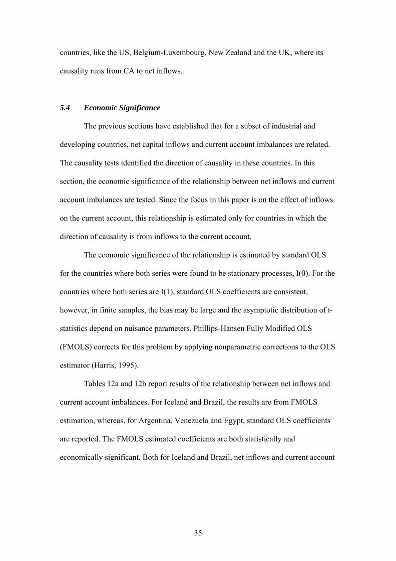
5.4 Economic Significance

The previous sections have established that for a subset of industrial and

developing countries, net capital inflows and current account imbalances are related.

The causality tests identified the direction of causality in these countries. In this

section, the economic significance of the relationship between net inflows and current

account imbalances are tested. Since the focus in this paper is on the effect of inflows

on the current account, this relationship is estimated only for countries in which the

direction of causality is from inflows to the current account.

The economic significance of the relationship is estimated by standard OLS

for the countries where both series were found to be stationary processes, I(0). For the

countries where both series are I(1), standard OLS coefficients are consistent,

however, in finite samples, the bias may be large and the asymptotic distribution of t-

statistics depend on nuisance parameters. Phillips-Hansen Fully Modified OLS

(FMOLS) corrects for this problem by applying nonparametric corrections to the OLS

estimator (Harris, 1995).

Tables 12a and 12b report results of the relationship between net inflows and

current account imbalances. For Iceland and Brazil, the results are from FMOLS

estimation, whereas, for Argentina, Venezuela and Egypt, standard OLS coefficients

are reported. The FMOLS estimated coefficients are both statistically and

economically significant. Both for Iceland and Brazil, net inflows and current account

35

imbalances are negatively correlated37. The standard OLS coefficients for Argentina,

Egypt and Venezuela are also negative, however, they are not statistically significant

at 10 percent significance level for Argentina and Egypt. For Venezuela the

coefficient for net inflows is economically significant, indicating that a unit increase

in net inflows causes a 1.16 unit current account deficit. The economic impact of net

inflows is also large in Iceland, but less than unity, where a unit increase in net

inflows causes 0.82 unit decrease in the current account imbalance. Compared to

Venezuela and Iceland, the economic impact of net inflows on the current account

imbalance in Brazil is moderate.

5.5 Summary

In summary, the cointegration and causality tests indicate that net inflows and

current account imbalances have a long-run steady-state relationship in a subset of

industrial and developing countries. The focus in this section was to answer the

question whether net inflows cause current account imbalances. Among the industrial

countries, there is evidence of causality running from net inflows to the current

account imbalance only in Iceland. Among the developing countries in our sample, in

Argentina, Brazil, Egypt and Venezuela net inflows cause current account imbalances.

Fry et al. (1995) also find evidence of capital account causing current account

imbalances in Argentina, Brazil and Venezuela for the period 1970-199238. Our

results indicate that the direction of the relationship in these countries remained stable

throughout the 1990s. Contrary to the results in this paper, Fry et al. (1995) show that

capital account and current account are independent in Egypt. The difference in

37 Both series are entered into the regression equation in levels. 38 The capital account in Claessens et al (1995) is equivalent to net inflows variable used in this study.

36

results may be based on the specific time periods captured. Most developing countries

progressively liberalized their capital account in the 1990s.

Fry et al. (1995) further investigate the predictability of the direction of

causality in their sample of 46 developing countries. They find that high levels of debt

(foreign and domestic) reduce the likelihood that capital account Granger-causes the

current account and increase the likelihood of no causality. This may explain our

results on Turkey, Morocco and Colombia. The existence of restrictions on capital

account payments reduces the likelihood of causality running from current account to

capital account. This may explain why in Singapore, and some industrial countries,

causality runs from current account to net inflows39. Overall, the balance-of-

payments regime of a country may define the causal relationship between its current

account and net inflows.

6. Conclusion

The relationship between international capital inflows and the current account

has been implied in the models of current account determination, and in the

‘sustainability’ literature, but this relationship has remained relatively unexplored.

This paper examined the relationship between net private capital inflows and the

current account in a set of industrial and developing countries. The aim of this paper

was to answer two specific questions regarding the relationship between net private

capital inflows and the current account. The first question asked whether the cyclical

volatility in current accounts could be explained by the volatility of capital flows. The

second question addressed the causal link between net capital inflows and current

account imbalances.

39 Singapore’s capital account is one of the most liberal among the developing countries.

37

The results indicate that country experiences vary. The evidence implies that

inflows do not cause current account imbalances in the industrial countries, nor does

the inflow volatility affect current account volatility. This may be explained due to the

fact that most industrial countries have liberalized capital accounts. Domestic markets

are open to foreign capital inflows and domestic agents are also free to invest abroad.

This may mean that in industrial countries, there are fewer barriers to borrowing and

lending internationally, compared to developing countries. Although, some

developing countries have undertaken structural reforms and liberalized their current

accounts, capital controls would have been prevalent for the most part of the time

period analysed. Such institutional barriers may be the reason why inflows cause

imbalances or volatility in the current account.

Another distinction between industrial and developing country current and

capital inflow dynamics may be based on their ability to borrow in the international

capital markets. Most industrial countries can borrow and lend freely, whereas most

developing countries are liquidity constrained. The ability to borrow in international

markets is restricted for developing countries, and mostly determined by foreign

investors’ willingness to lend. During an economic downturn, sudden reversals in

inflows can induce a liquidity crisis. This may explain the relationship between

volatility in inflows and current accounts in developing countries.

Finally, it is worth remembering the consumption-smoothing hypothesis of the

current account. The consumption-smoothing approach combines the assumptions of

high capital mobility and permanent income theory of consumption in a small, open

economy to predict what capital flows would be if agents behave in accordance with

the permanent income theory. According to this approach, a country’s current account

will be in deficit whenever national cash flow, is expected to rise over time. It will be

38

in surplus whenever national cash flow is expected to fall. One important implication

of this theory is that all countries are expected to behave the same under the same

circumstances. Our results indicate that the experience of the industrial and

developing countries are quite different. This may be closely linked to the fact that

developing countries are credit-constrained in contrast with industrial countries.

This paper shows that the behaviour of the capital inflows is different in

industrial countries compared to developing countries. This implies that comparative

research on the consumption smoothing effects of capital inflows in industrial versus

developing countries would be worthwhile.

Acknowledgements

This work was carried out as part of the PhD thesis of the author at Trinity College

Dublin. The author is grateful to Philip Lane for invaluable comments at various

stages of this work and to the participants of International Economics workshops in

Trinity College Dublin, Spring Meeting of Young Economists 2003 in Leuven for

useful discussions. The author acknowledges financial support from the Irish

Research Council for the Humanities and Social Sciences.

39

Appendix

List of Countries

Industrial Countries Developing Countries

Australia (AUS) Argentina (ARG)

Austria (AUT) Brazil (BRA)

Belgium-Luxembourg (BEL) Chile (CHL)

Canada (CAN) China (CHN)

Denmark (DEN) Colombia (COL)

Finland (FIN) Costa Rica (CRI)

France (FRA) Egypt (EGY)

Germany (GER) India (IND)

Iceland (ICE) Indonesia (IDN)

Italy (ITA) Israel (ISR)

Japan (JAP) Korea (KOR)

Netherlands (NET) Malaysia (MYS)

Norway (NOR) Mexico (MEX)

New Zealand (NZL) Morocco (MAR)

Portugal (PRT) Philippines (PHL)

Spain (ESP) Singapore (SGP)

Sweden (SWE) Thailand (THA)

Switzerland (SWI) Turkey (TUR)

United Kingdom (UK) Venezuela (VEN)

40

United States (US)

41

References

Aizenman, J., Marion, N., 2002. The High Demand for International Reserves in the

Far East: What is going on?. National Bureau of Economic Research, Working

Paper no.9266.

Bacchetta, P., Wincoop E., 1998. Capital Flows to Emerging Markets: Liberalization,

Overshooting and Volatility. National Bureau of Economic Research,

Working Paper no 6530.

Baltagi, B., 1999. Econometric Analysis of Panel Data. John Wiley and Sons Ltd.,

West Sussex.

Baxter, M., King, G., 1995. Measuring Business Cycles: Approximate Band-Pass

Filters for Economic Time Series. National Bureau of Economic Research,

Working Paper no.5022.

Bosworth, B., Collins, S., 1999. Capital Flows to Developing Economies:

Implications for Savings and Investment. Brookings Papers on Economic

Activity, 1.

Caballero, R., Krishnamurthy , A., 2001. International Liquidity Illusion: On the

Risks of Sterilization. National Bureau of Economic Research, Working Paper

no. 8141.

Calderon, C., Chong, A., Loayza, N., 2002. Determinants of Current Account Deficits

in Developing Countries, Latin American and Caribbean Economic

Association, conference proceedings.

Calvo, G., Leiderman, L., Reinhart, C., 1996. Inflows of Capital to Developing

Countries in the 1990s. Journal of Economic Perspectives, 10, 123-139,

Spring.

42

Calvo, G., Vegh, C., 1993. Exchange Rate Based Stabilization Under Imperfect

Credibility, In: Frisch, H., Worgotter, A., (Eds.), Open Economy

Macroeconomics, Basingstoke.

Chinn, M., Prasad, E. S., 2000. Medium-Term Determinants of Current Accounts in

Industrial and Developing Countries: An Empirical Exploration. IMF Working

Paper, no. 46.

Claessens, S., Dooley, M., Warner, A., 1995. Portfolio Capital Flows:Hor or Cold?.

The World Bank Economic Review, 9, 153-174.

Cochrane, J. H., 1988. How Big is the Random Walk in GNP?. The Journal of

Political Economy, 96, 5, 893-920.

Davidson, R., MacKinnon, J. G., 1993. Estimation and Inference in Econometrics,

Oxford University Press.

Enders, W., 1995. Applied Econometric Time Series, John Wiley and Sons, New

York.

Feldstein, M., Horioka, C., 1980. Domestic Saving and International Capital Flows.

Economic Journal, vol 90, 314-329.

Freund, C., 2000. Current Account Adjustment in Industrialized Countries.

International Finance Discussion Papers no. 692, Board of Governors of the

Federal Reserve System.

Fry, M., Claessens, S., Burridge, P., Blanchet, M., 1995. Foreign Direct Investment,

Other Capital Flows and Current Account Deficits: What causes what?. World

Bank Policy Research Working Paper no. 1527.

43

Ghosh, A., Ostry, J. D., 1993. Do Capital Flows Reflect Economic Fundamentals in

Developing Countries?. IMF Working Paper, 93/34.

Ghosh, A., Ostry, J. D., 1995. The Current Account in Developing Countries : A

Perspective from The Consumption Smoothing Approach. World Bank

Economic Review, no 9.

Goldstein, M., Mathieson, D. J., Lane, T., 1994. Determinants of Systemic

Consequences of International Capital Flows. International Capital Markets,

IMF.

Guay, A., St-Amant, P., 1997. Do the Hodrick-Prescott and Baxter-King Filters

Provide a Good Approximation of Business Cycles?. Center for Research on

Economic Fluctuations and Employment Working Paper no.53.

Gujarati, D. N., 1995. Basic Econometrics, McGraw Hill, Singapore.

Harris, R. I. D., 1995. Using Cointegration Analysis in Econometric Modelling,

Prentice Hall, London.

Harvey, A.C., Jaeger, A., 1993. Detrending, Stylized Facts and the Business Cycle.

Journal of Applied Econometrics, 8, 231-247.

Hutchison, M., Noy, I., 2002. Sudden Stops and the Mexican Wave: Currency Crises,

Capital Flow Reversals and Output Loss in Emerging Markets. 4th Conference

of the Analysis if International Capital Markets Research Training Network

proceedings, Dublin, December.

IMF, 1999. World Economic Outlook, October, pp.62-64.

Johnston, B., Tamirisa, N., 1998. Why Do Countries Use Capital Controls?, IMF

Working Paper, no.181.

King, R.G., Rebello, S., 1993. Low Frequency Filtering and Real Business Cycles.

Journal of Economic Dynamics and Control, 17, 207-231.

44

Kraay, A., Ventura, J., 2000. Current Accounts in Debtor and Creditor Countries.

Quarterly Journal of Economics, XCV (2000), 1137-1166.

Kraay, A., Ventura, J., 2002. Current Accounts in the Long and Short-Run. Latin

American and Caribbean Economic Association, meeting proceedings.

Kwiatkowski, D., Phillips, P.C., Schmidt, P., Shin, Y., 1992. Testing the Unit Root

Hypothesis of Stationarity Against the Alternative of a Unit Root. Journal of

Econometrics, 152-178.

Lane, P., Milesi-Ferretti, G.M., 2001. Long-Term Capital Movements. National

Bureau of Economic Research, Working Paper no 8366.

Lane, P., Burke, D., 2001. The Empirics of Foreign Reserves. Open Economies

Review, 12(4), October.

MacKinnon, J.G., 1991. Critical Values for CointegrationTests. In: Engle, R.F.,

Granger, C.W.J., (Eds.), Long-Run Economic Relationship: Readings in

Cointegration, Chapter 13, Oxford University Press.

Meade, J., 1951. The Balance of Payments, London, Oxford University Press.

Milesi-Ferretti, G., Razin, A., 1996a. Current Account Sustainability. Princeton

Essays in International Finance, no 81.

Milesi-Ferretti, G., Razin A., 1996b. Current Account Sustainability: Selected East

Asian and Latin American Experiences. National Bureau of Economic

Research, Working Paper no 5791.

Milesi-Ferretti, G., Razin, A., 1998. Sharp reductions in current account deficits; An

empirical analysis. European Economic Review, 42, 897-908.

45

Milesi-Ferretti, G., Razin, A., 1999. Current Account Reversals and Currency Crises;

Empirical Regularities. In: Krugman, P. (ed.), Currency Crises, University of

Chicago Press.

Osei, R., Morrisey, O., Lensink, R. 2000. The Volatility of Capital Inflows: Measures

and Trends for Developing Countries, CREDIT Research Paper 7836, 02/20.

Said, E., Dickey, D., 1984. Testing for Unit Roots in Autoregressive Moving Average

Model of Unknown Order. Biometrika, 71, 599-607.

Sarno, M., Taylor, L., 1997. Hot-Money, Accounting Labels and the Persistence of

Capital Flows to Developing Countries: An Empirical Investigation.

Discussion Paper, 7, Brunel University.

Turner, P., 1991. Capital Flows in the 1980s: A survey of major trends. Economic

Papers, no.30, Bank for International Settlements, Basle.

Verbeek, M., 1999. A Guide to Modern Econometrics, John and Wiley Sons.

World Bank, 1999, Global Development Finance, Ch 3, 47-67.

46

Table 1a Current Account Volatility – Industrial Countries Volatility CA Inflows Outflows Reserve Net

Inflows Year

Australia 0.012 0.013 0.007 0.013 0.012 1960-2000

Austria 0.012 0.023 0.024 0.010 0.012 1967-2000

BEL 0.011 0.209 0.210 0.007 0.012 1975-2000

Canada 0.012 0.017 0.014 0.006 0.012 1948-2000

Denmark 0.014 0.053 0.050 0.025 0.028 1975-2000

Finland 0.020 0.038 0.032 0.019 0.027 1975-2000

France 0.007 0.029 0.028 0.006 0.007 1975-2000

Germany 0.013 0.016 0.023 0.008 0.016 1971-2000

Iceland 0.021 0.026 0.012 0.010 0.013 1976-2000

Italy 0.015 0.020 0.020 0.013 0.024 1970-2000

Japan 0.010 0.016 0.016 0.006 0.010 1977-2000

Netherlands 0.014 0.042 0.037 0.007 0.016 1967-2000

New Zealand 0.031 0.023 0.017 0.023 0.022 1972-2000

Norway 0.037 0.034 0.033 0.026 0.032 1975-2000

Portugal 0.035 0.034 0.028 0.026 0.037 1975-2000

Spain 0.016 0.037 0.037 0.020 0.020 1975-2000

Sweden 0.013 0.047 0.031 0.017 0.026 1970-2000

Switzerland 0.014 0.061 0.071 0.019 0.024 1977-1999

UK 0.013 0.078 0.075 0.014 0.016 1970-2000

US 0.008 0.011 0.008 0.001 0.009 1970-2000

Notes: All variables are expressed as a ratio to GDP. The volatility measure is the standard deviation of HP(100) filtered series.

47

Table 1b Current Account Volatility – Developing Countries Volatility CA Inflows Outflows Reserve Net

Inflows Year

Argentina 0.020 0.033 0.011 0.031 0.031 1976-2000

Brazil 0.012 0.017 0.005 0.017 0.016 1975-2000

Chile 0.028 0.069 0.026 0.061 0.063 1975-2000

China 0.020 0.014 0.009 0.017 0.017 1982-2000

Colombia 0.029 0.021 0.007 0.018 0.021 1968-2000

Costa Rica 0.024 0.027 0.014 0.034 0.032 1977-1999

Egypt 0.026 0.049 0.020 0.055 0.059 1977-2000

India 0.006 0.006 0.004 0.008 0.005 1975-2000

Indonesia 0.020 0.027 0.001 0.015 0.037 1981-1999

Israel 0.030 0.029 0.022 0.031 0.029 1952-2000

Korea 0.040 0.032 0.011 0.024 0.028 1976-1999

Malaysia 0.061 0.047 0.025 0.048 0.055 1974-1999

Mexico 0.025 0.028 0.013 0.027 0.032 1979-2000

Morocco 0.027 0.043 0.005 0.019 0.043 1975-1999

Philippines 0.033 0.033 0.048 0.031 0.043 1977-2000

Singapore 0.031 0.108 0.103 0.022 0.048 1972-2000

Thailand 0.035 0.039 0.007 0.027 0.042 1975-2000

Turkey 0.015 0.022 0.010 0.011 0.019 1974-2000

Venezuela 0.069 0.032 0.020 0.044 0.035 1970-2000

Notes: All variables are expressed as a ratio to GDP. The volatility measure is the standard deviation of HP(100) filtered series.

48

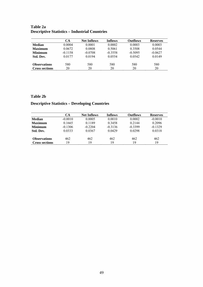
Table 2a Descriptive Statistics – Industrial Countries

CA Net Inflows Inflows Outflows Reserves Median 0.0004 0.0001 0.0002 0.0003 0.0003 Maximum 0.0672 0.0808 0.5061 0.3508 0.0544 Minimum -0.1158 -0.0708 -0.3558 -0.5095 -0.0627 Std. Dev. 0.0177 0.0194 0.0554 0.0542 0.0149

Observations 580 580 580 580 580 Cross sections 20 20 20 20 20 Table 2b

Descriptive Statistics – Developing Countries

CA Net Inflows Inflows Outflows Reserves

Median -0.0010 0.0005 0.0010 0.0002 -0.0010 Maximum 0.1665 0.1189 0.3458 0.2144 0.2096 Minimum -0.1306 -0.2204 -0.3136 -0.3399 -0.1329 Std. Dev. 0.0333 0.0367 0.0429 0.0298 0.0318

Observations 462 462 462 462 462 Cross sections 19 19 19 19 19

49

Table 3 Fixed-Effects Estimation on Current Account Volatility

Dependent Variable: (CA) volatility

(1) Industrial countries

(2) Developing countries

Net Inflow volatility 0.17

(1.38) 0.35

(5.13)*** N 109 91 Adj R2 0.42 0.65 s.e 0.008 0.01 *, **, and *** indicate statistical significance at 10, 5 and 1 percent level.

Table 4 OLS Panel Estimation on Current Account Volatility

Dependent Variable: (CA) volatility

(1) Industrial countries

(2) Developing countries

Net Inflow volatility 0.47

(4.74)*** 0.40

(3.77)*** N 109 91 Adj R2 0.27 0.21 s.e 0.01 0.02 *, **, and *** indicate statistical significance at 10, 5 and 1 percent level.

50

Table 5 Robustness Checks- Panel Fixed-Effects Estimation (Outliers excluded)

Dependent Variable: (CA) volatility

(1) Industrial countries

(2) Developing countries

Net Inflow volatility 0.20

(3.13)*** 0.37

(5.61)*** N 94 87 Adj R2 0.66 0.77 s.e 0.005 0.008

*, **, and *** indicate statistical significance at 10, 5 and 1 percent level.

Table 6 Fixed-Effects Estimation on Reserve Volatility

Dependent Variable:

(RES) volatility (1)

Industrial countries

(2) Developing countries

Net Inflow volatility 0.43

(3.41)*** 0.57

(4.05)*** N 109 91 Adj R2 0.49 0.55 s.e 0.007 0.01

51

Table 7 Robustness Checks- Panel Fixed-Effects Estimation (Outliers excluded)

Dependent Variable: (RES) volatility

(1) Industrial countries

(2) Developing countries

Net Inflow volatility 0.28

(4.03)*** 0.49

(3.84)*** N 105 89 Adj R2 0.63 0.56 s.e 0.005 0.01

*, **, and *** indicate statistical significance at 10, 5 and 1 percent level.

52

Table 8a Unit Root Tests (Augmented Dickey Fuller test) Sample: Industrial Countries

CA ∆CA Net Inflow ∆Net Inflow Period Australia -1.77 -5.37*** -3.30** 1960-2000 Austria -2.45 -6.16*** -1.76 -8.16*** 1967-2000 BEL -0.05 -3.51*** -0.42 -3.26*** 1975-2000 Canada -2.86* -3.68*** 1948-2000 Denmark -2.00** -1.13 -8.48*** 1975-2000 Finland -1.09 -3.72*** -3.11*** 1975-2000 France -1.78* -1.38 -5.59*** 1975-2000 Iceland -1.91 -5.88*** -2.04 -5.08*** 1976-2000 Germany -1.58 -4.25*** -2.19*** 1971-2000 Italy -2.79*** -2.38 -3.52*** 1970-2000 Japan -3.68** -4.11*** 1977-2000 Netherlands -2.55 -5.97*** -4.58*** 1967-2000 New Zealand -2.75* -2.22** 1972-2000 Norway -2.42 -3.62*** -3.10*** 1975-2000 Portugal -2.57 -4.28*** -3.17** 1975-2000 Spain -4.08*** -3.38** 1975-2000 Sweden -1.89* -2.98*** 1970-2000 Switzerland 2.28 -6.50*** -1.69 -1.36 1977-1999 UK -2.99** -2.51** 1970-2000 US 0.33 -3.90*** -1.27 -6.01*** 1970-2000 Table 8b Unit Root Tests (Augmented Dickey Fuller test) Sample: Developing Countries CA ∆CA Net Inflow ∆Net Inflow Period Argentina -4.10*** -2.36** 1976-2000 Brazil -1.43 -4.56*** -1.41 -4.85*** 1975-2000 Chile -0.75 -5.84*** -2.40** 1975-2000 China -2.55** -2.10 -4.67*** 1982-2000 Colombia -3.10** -2.67* 1968-2000 Costa Rica -1.48 -6.43*** -2.12** 1977-1999 Egypt -2.17** -3.01*** 1977-2000 India -3.53** -2.22 -7.45*** 1975-2000 Israel -2.00 -7.34*** -3.31** 1952-2000 Korea -2.06** -1.93* 1976-1999 Malaysia -2.57** -1.70* 1974-1999 Mexico -2.34 -2.54** -3.06** 1979-2000 Morocco -2.60** -3.60*** 1975-1999 Philippines -1.73* -1.29 -4.41*** 1977-2000 Singapore -0.40 -3.82*** -1.41 -5.29*** 1972-2000 Thailand -1.47 -4.52*** -1.86* 1975-2000 Turkey -1.84* -4.93*** 1974-2000 Venezuela -5.32*** -2.15** 1970-2000 Notes: All variables are expressed as a ratio to GDP. The lag length and the choice to include a constant or not are based on AIC. The test statistics (τ) are significant at 1 percent (***), 5 percent (**) and 10 percent (*).

53

54

Table 9a Engle-Granger and Johansen Cointegration Tests Cointegrating regression: CA = a + b(Inflw) Sample: Industrial Countries (1)

ADF Test Statistic

(2) Number of Lags

(3) λtrace

Austria -4.22*** 0 29.52*** Belgium-Luxembourg -3.79*** 0 13.36 Iceland -4.01*** 3 20.33** US -2.61** 1 9.80

Notes: All cointegrating models include a constant. ADF test includes no constant and no trend. Table 9b Engle-Granger and Johansen Cointegration Tests Cointegrating regression: CA = a + b(Inflw) Sample: Developing Countries (1)

ADF Test Statistic

(2) Number of Lags

(3) λtrace

Brazil -2.70*** 0 13.19 Singapore -3.37*** 2 14.96 Notes: All cointegrating models include a constant. ADF test includes no constant and no trend.

Table 10a Standard Granger Causality tests Sample: Industrial countries Y Yt-1 Yt-2 Yt-3 Xt-1 Xt-2 Xt-3 F-stat DecisionCanada CA

Net Inflows

0.59 (2.27)** 0.35 (1.30)

0.04(0.16) -0.07 (-0.27)

0.03 0.05

Independent

Japan CA Net Inflows

0.44 (1.77)* 0.02 (0.08)

-0.24 (-0.70)

-0.39 (-1.52) -1.05 (-2.56)**

0.51 (1.56)

2.31 3.68**

CA⇒Inflw

New Zealand

CA Net Inflows

0.56 (3.77)*** 0.58 (3.73)***

0.09(0.48) 0.26 (1.82)*

-0.29 (-1.52)

0.19 (1.03)

0.84 3.30***

CA⇒Inflw

Spain CA Net Inflows

0.87 (3.83)*** 0.26 (1.22)

-0.28 (-0.98)

-0.27 (-1.24)

-0.01 (-0.10) -0.21 (-0.77)

0.01 0.60

Independent

Sweden CA Net Inflows

0.77 (4.95)*** 0.51 (2.75)***

0.02(0.26) -0.06 (-0.22)

0.07 0.05

Independent

UK CA Net Inflows

0.57 (3.22)*** 0.06 (0.24)

-0.20(-1.26) -0.54 (-1.93)*

1.60 3.73***

CA⇒Inflw

55

Table 10b: Standard Granger Causality tests (Sample: Developing countries)

Y Yt-1 Yt-2 Yt-3 Xt-1 Xt-2 Xt-3 F-stat DecisionArgentina CA

Net Inflows

0.22 (1.42) 0.63 (3.27)***

-0.22 (-1.43)

0.06 (0.42)

-0.36 (-4.58)*** 0.35 (1.15)

20.96*** Inflw⇒CA 1.33

Colombia CA Net Inflows

0.34 (1.36) 0.55 (2.01)**

-0.55(-1.60) -0.19 (-0.84)

0.24 (1.66)

2.56 1.37

Independent

Egypt CA Net Inflows

-0.31 (-1.47) 0.39 (1.70)

-0.36(-3.98)*** -0.11 (-0.30)

-0.22 (-2.60)**

-0.23 (-2.58)**

8.81*** 0.09

Inflw⇒CA

Korea CA Net Inflows

-0.20 (-0.79) 1.09 (4.09)***

-1.24(-4.00)*** 0.39 (1.82)*

15.99*** CA⇔Inflw 3.31*

Malaysia CA Net Inflows

0.55 (1.99)* 0.28 (1.01)

-0.19 (-0.59)

-0.40 (-1.49)

-0.42 (-1.32) -0.46 (-1.81)*

1.74 3.28***

CA⇒Inflw

Morocco CA Net Inflows

0.51 (2.55)** 0.82 (3.26)***

-0.40 (-1.68)

0.19 (1.37)

-0.27 (-1.18) -0.10 (-0.48)

0.34 (1.56)

-0.32 (-2.48)**

2.15 0.23

Independent

Turkey CA Net Inflows

0.27 (1.04) 0.08 (0.33)

-0.29 (-1.30)

0.41 (1.97)*

0.33 (1.40) 0.47 (1.68)

1.97 2.83

Independent

Venezuela CA Net Inflows

0.05 (0.23) 0.67 (3.15)***

-0.20 (-0.95)

-0.30 (-1.61)

-0.75 (-1.85)* 0.16 (1.53)

3.42*** Inflw⇒CA 2.33

56

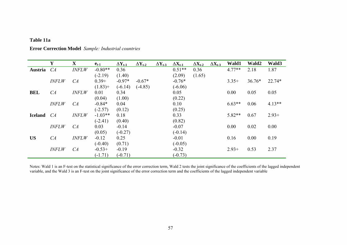
Table 11a

Error Correction Model Sample: Industrial countries

Y X et-1 ∆Yt-1 ∆Yt-2 ∆Yt-3 ∆Xt-1 ∆Xt-2 ∆Xt-3 Wald1 Wald2 Wald3Austria CA INFLW -0.80**

(-2.19) 0.36 (1.40)

0.51** 0.36 (2.09) (1.65)

4.77** 2.18 1.87

INFLW

CA 0.39+ (1.83)+

-0.97* (-6.14)

-0.67* (-4.85)

-0.76* (-6.06)

3.35+ 36.76* 22.74*

BEL CA INFLW 0.01 (0.04)

0.34 (1.00)

0.05(0.22)

0.00 0.05 0.05

INFLW CA -0.84* (-2.57)

0.04 (0.12)

0.10(0.25)

6.63** 0.06 4.13**

Iceland CA INFLW -1.03** (-2.41)

0.18 (0.40)

0.33(0.82)

5.82** 0.67 2.93+

INFLW CA 0.03 (0.05)

-0.14 (-0.27)

-0.07 (-0.14)

0.00 0.02 0.00

US CA INFLW -0.12 (-0.40)

0.25 (0.71)

-0.01 (-0.05)

0.16 0.00 0.19

INFLW CA -0.53+ (-1.71)

-0.19 (-0.71)

-0.32 (-0.73)

2.93+ 0.53 2.37

Notes: Wald 1 is an F-test on the statistical significance of the error correction term, Wald 2 tests the joint significance of the coefficients of the lagged independent variable, and the Wald 3 is an F-test on the joint significance of the error correction term and the coefficients of the lagged independent variable

57

58

Table 11b Error Correction Model Sample: Developing countries

Y X et-1 ∆Yt-1 ∆Yt-2 ∆Yt-3 ∆Xt-1 ∆Xt-2 ∆Xt-3 Wald1 Wald2 Wald3Brazil CA INFLW -0.60*

(-3.04) 0.22 (1.14)

0.08(0.39)

9.24* 0.15 6.56*

INFLW

CA 0.41 (1.19)

-0.35 (-1.44)

-0.18 (-0.82)

1.41 0.67 0.93

Singapore CA INFLW -0.20 (-1.58)

-0.19 (-1.09)

-0.02 0.17 (-0.12) (1.36)

2.51 1.39 2.03

INFLW CA -0.48* (-3.05)

0.20 (1.03)

0.62** 0.18 (2.57) (0.58)

9.31* 0.53 4.51*

Notes: Wald 1 is an F-test on the statistical significance of the error correction term, Wald 2 tests the joint significance of the coefficients of the lagged independent variable, and the Wald 3 is an F-test on the joint significance of the error correction term and the coefficients of the lagged independent variable

Table 12a Fully Modified OLS estimation CAt = α +β(Inflow)t

Note: Bartlett Weights, 2 lags, no trend. t-statistics in parantheses.

Country β Sample Period Iceland -0.82 (-8.89)*** 1977-2000 Brazil -0.55 (-4.91)*** 1975-2000

Significance levels at 1, 5 and 10 percent are indicated by ***, **, *. Table 12b OLS estimation CAt = α +β(Inflow)t

Country β R2 DW Sample PeriodArgentina -0.12 (-1.27) 0.28 1.87 1977-2000 Egypt -0.19 (-1.66) 0.51 1.98 1977-1999 Venezuela -1.16 (-3.68)*** 0.37 1.75 1970-2000 Note: Newey-West heteroskodasticity and autocorrelation consistent t-statistics in parantheses. Significance levels at 1, 5 and 10 percent are indicated by ***, **, *. AR(1) correction included.

59

60

Figure 1.1 CA, Inflows and Outflows : Industrial Countries

-0.3

-0.2

-0.1

0

0.1

0.2

0.3

1963

1966

1969

1972

1975

1978

1981

1984

1987

1990

1993

1996

1999

CA/GDP Outflows/GDP Inflows/GDP

Figure 1.2 CA, Inflows, Outlfows : Developing Countries

-0.08-0.06-0.04-0.02

00.020.040.060.080.1

0.12

1967

1969

1971

1973

1975

1977

1979

1981

1983

1985

1987

1989

1991

1993

1995

1997

1999

CA/GDP Inflows/GDP Outflows/GDP

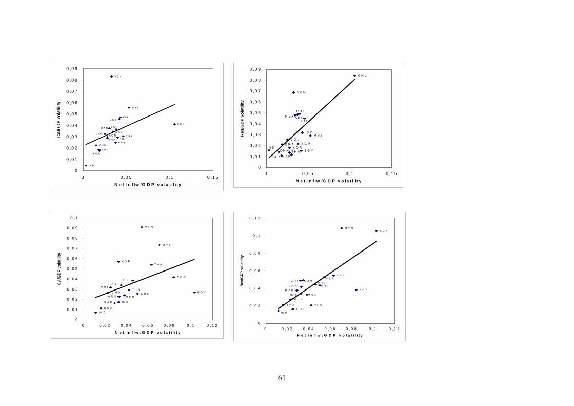
C H N

M A RT H A

T U R

E G YK O RIN D

B R A S G PC O L

M Y SIS R

A R GM E XC R I

P H L

V E N

C H L

0

0 ,0 1

0 ,0 2

0 ,0 3

0 ,0 4

0 ,0 5

0 ,0 6

0 ,0 7

0 ,0 8

0 ,0 9

0 0 ,0 5 0 ,1 0 ,1 5

N e t In f lw /G D P v o la t i l i t y

Res

/GD

P vo

latil

ity

B R AT U R

C R IP H LT H A

A R GC H N

C O L M E XK O R

S G PM A RC H L

E G YIS R

M Y S

V E N

IN D

0

0 ,0 1

0 ,0 2

0 ,0 3

0 ,0 4

0 ,0 5

0 ,0 6

0 ,0 7

0 ,0 8

0 ,0 9

0 0 ,0 5 0 ,1 0 ,1 5

N e t In f lw /G D P v o la t i l i t y

CA

/GD

P vo

latil

ity

C R I

K O R

T H A

C H LP H L

K O R

I S RM A R

B R A T U R

C H N

C O L

M E X

V E N

I N D

S G P

E G YM Y S

0

0 , 0 2

0 , 0 4

0 , 0 6

0 , 0 8

0 , 1

0 , 1 2

0 0 , 0 2 0 , 0 4 0 , 0 6 0 , 0 8 0 , 1 0 , 1 2

N e t I n f l w / G D P v o l a t i l i t y

Res

/GD

P vo

latil

ity

V E N

M Y S

K O RT H A

S G P

E G YC H L

IN D

M A R

B R A

T U R

P H L

C O L

M E X

C R I

C H N

IS R

A R G

0

0 , 0 1

0 , 0 2

0 , 0 3

0 , 0 4

0 , 0 5

0 , 0 6

0 , 0 7

0 , 0 8

0 , 0 9

0 , 1

0 0 , 0 2 0 , 0 4 0 , 0 6 0 , 0 8 0 , 1 0 , 1 2

N e t In f l w / G D P v o l a t i l i t y

CA

/GD

P vo

latil

ity

61

F ig u re 4 (B ): V o la tility in R e s e rv e s a n d In flo w s :

In d u s tr ia l C o u n tr ie s (1 9 8 0 s )

A U T

F IN

G E RN E TU KB E L

A U S

C A N

IT A

IC EN Z L S W IE S P

S W E

J A PF R A

U S

D E NN O R

P R T

0

0 .0 1

0 .0 2

0 .0 3

0 .0 4

0 .0 5

0 .0 6

0 0 .0 2 0 .0 4 0 .0 6 0 .0 8

N e t In flw /G D P vo la tility

Res

/GD

P vo

latil

ity

Figure 4 (D):

Volatility in Reserves and Inflows: Industrial Countries (1990s)

DENNOR

ESP FINPRT

SWENZL

ICE

USSWI

AUTAUS

GERITA

FRAUK

JAP NETCAN

BEL0

0.01

0.02

0.03

0.04

0.05

0.06

0 0.01 0.02 0.03 0.04 0.05 0.06Net Inflw/GDP volatility

Res

/GD

P vo

latil

ity

62

F i g u r e 4 ( C ) : V o l a t i l i t y i n C A a n d I n f l o w s : I n d u s t r i a l C o u n t r i e s ( 1 9 9 0 s )

I C E

N O R

P R T

A U T

N E T N Z L

F I NE S PD E N

S W E

U SF R A

U K

S W II T A G E R

J A PB E L

C A NA U S

0

0 . 0 1

0 . 0 2

0 . 0 3

0 . 0 4

0 . 0 5

0 . 0 6

0 0 . 0 1 0 . 0 2 0 . 0 3 0 . 0 4 0 . 0 5 0 . 0 6

N e t I n f l w / G D P v o l a t i l i t y

CA

/GD

P vo

latil

ity

Figure 4(A):Volatility in Current Account and Inflows:

Industrial Countries (1980s)

AUSBELFRA

CAN

GER

DENNETESP

SW E

JAP

ICE

AUT

UK

US

ITA FIN

SW I

NZL

NOR

PRT

0

0.01

0.02

0.03

0.04

0.05

0.06

0 0.01 0.02 0.03 0.04 0.05 0.06 0.07

Net Inflw/GDP volatility

CA

/GD

P vo

latil

ity

63