
Finite element analysis of ground deformation due to dike ...

The Reduced Basis Method for a Finite Deformation Problem
Lorenzo ZanonKaren Veroy-Grepl
Advisory Board MeetingRWTH Aachen University
July 12, 2011
Aachen Institute for Advanced Studyin Computational Engineering Science
AICES Progress since 2009
• Overview of the AICES project
• New Principal Investigators
• New Young Researchers
• New facilities
• Recent highlights
• Goals and schedule of Advisory Board meeting
Outline
2
• Excellence Initiative Graduate School
• First period Nov 2006–Oct 2012
• Annually 1 M! + overhead
• Proposed for 2013–2017
• Funded personnel growth:
Overview of the AICES Project
3
0
4
8
12
16
20
24
28
32
36
40
1 3 3 3 3 3 3
1 1 3 3 4 41
1 1 1 11
6
912
18 201
4
72
2
02/200712/2007
12/200812/2010
Service Team
Junior Research Group Leaders
Adjunct Professors
Doctoral Fellows
Master Students
Postdoctoral Research Associates
• Computational engineering science is maturing
• “Old” challenges are still here:• complexity increasing intricacy of analyzed systems• multiscale interacting scales considered at once• multiphysics interacting physical phenomena
• AICES concentrates on areas of synthesis:• model identification and discovery supported by
model-based experimental analysis (MEXA)• understanding scale interaction and scale integration• optimal design and operation of engineered systems
• Inspiration: Collaborative Research Center 540• established in 1999, continued until 2009• Marquardt: coordinator, 6 AICES PIs: project leads
Overview of AICES Academic Aims
SFB 540
4
3rd ECCOMAS Young Investigators Conference YIC2015July 21, 2015

Outline
1. Motivation2. The Reduced Basis Method3. Fundamental Equations in Elasticity4. Numerical Example: Finite Deformation5. Conclusion
Lorenzo Zanon

Part 1 - Motivation
Dimension reduction:PDE Description in a continuous setting of the physics of the problem:
I field variable: displacement, temperature, . . .I output of interest: flow-rate, mean quantity, heat flux, critical load, . . .
FE Highly accurate approximation:I high accuracy, truth solution;I offline dimension N = O(103), expensive computations.
RB Built upon FE, in a parametric context:I m.o.r. even for complex nonlinear models;I online dimension N = O(10);I drastic reduction of computation times:
I parameter identification / inverse problems;I control and optimization;I many-query / real-time context.
Lorenzo Zanon 1/21

Motivation
RB Method in the context of elasticity can be applied to:I the description of the nonlinear behavior of materials
in finite deformation regime. Possible future applications:I rubber-like materials;I biological tissues.
I the analysis of buckling structures characterized byparameter-dependent geometries
→ truss systems
Lorenzo Zanon 2/21

Motivation
State of the art:I Successful application of the RB Method to linearized elasticity;I Other model order reduction techniques for nonlinear elasticity→ Proper Orthogonal Decomposition, SVD-based approach:
+ Dealing with complex problems (viscoelasticity, plasticity, . . . );+ Processing results pre-obtained from existent softwares (FEAP)
with POD-related techniques (DEIM, substructuring);+ Good results in terms of CPU-ratio and precision w.r.t. FE;
− Lack of an efficient greedy procedure to select snapshots;− Parametric nature of the problem only partially exploited;− No clear offline-online distinction; always N -dependent problems.
I RB for nonlinear elasticity currently under investigation.
Lorenzo Zanon 3/21
A. Radermacher, S. Reese, POD-based model reduction for nonlinearbiomechanical analysis. Int. J. of Materials Engineering Innovation, 2013.

Outline
1. Motivation2. The Reduced Basis Method3. Fundamental Equations in Elasticity4. Numerical Example: Finite Deformation5. Conclusion
Lorenzo Zanon

Part 2 - The RB MethodI Weak-formulation of a parametrized boundary-value problem:
a(u(µ),v; µ) = f (v; µ) , ∀v ∈V ⊂ H1(Ω) ;
a(v,v; µ) : V ×V → R , f (v; µ) : V → R , bilinear resp. linear forms.I The parameters µ ∈D ⊂ Rd can be of geometric or physical nature;
With the RB method, the FE solution - dim. N = O(103) -is projected on a low-dimensional space - dim. N = O(10).
I Build up the RB space by taking snapshots at well-chosen parameters:
ZN = span(u(x; µ j)); j = 1, . . . ,Nmax= span(ζ j(x)); j = 1, . . . ,Nmax
I . . . selected through a greedy procedure:for N = 1, . . . ,Nmax
µ∗N = argmaxµ∈D train
∆uN−1(µ)e(u)N−1(µ)
⇒ ZN = ZN−1∪ spanu(µ∗N) .
Lorenzo Zanon 4/21
C. Prud’homme, D. V. Rovas, K. Veroy, L. Machiels, Y. Maday, A. T. Patera, and G. Turinici. Reliable real-time
solution of parametrized PDEs: Reduced-basis output bound methods. J. of Fluids Engineering, 2002.

The RB Method - Offline/OnlineWhy use the RB Method in a parametrized context?
I Offline phase: the FE-dependent quantities are computed and stored;I Online phase: the parameter-dependent low-dimensional system is
solved.
I Separability of the linear forms in the truth FE setting
a(w,v; µ) =Qa
∑q=1
Θq(µ)aq(w,v) ;
. . . maintained in the RB setting: a(vN ,wN ; µ) =Qa
∑q
Θq(µ)aq(vN ,wN) .
I Nonaffine problems: use interpolation techniques, e.g. EIM.For N ≤ Nmax, we obtain the RB approximation . . .
I of the solution: u(µ)≈ uN(µ) :=N
∑j=1
uN j(µ)ζ j;
I of an output of interest: s(µ)≈ sN(uN(µ)).
Lorenzo Zanon 5/21

Outline
1. Motivation2. The Reduced Basis Method3. Fundamental Equations in Elasticity4. Numerical Example: Finite Deformation5. Conclusion
Lorenzo Zanon

Part 3 - Fundamental Equations in Elasticity
Deformation of bodies with a defined shape:→ Elasticity: the original shape is recovered once the stress ceases its action.← yielding / plasticity / fracture / . . .
Equilibrium Equation: σϕ
i j, j +bϕ
i = 0 , in Ωϕ ⊂ Rd ;Momentum Equation: σ
ϕ
i j = (σϕ
i j )t , in Ωϕ ⊂ Rd ;
Dirichlet Conditions: ui = ui , on δΩϕ,D ⊂ Rd−1 ;Applied Traction: σ
ϕ
i j nϕ
j = T ϕ
i , on δΩϕ,T ⊂ Rd−1 ;
I Here:u : unknown displacement;σ := σ(u) : Cauchy stress matrix;b : volumetric forces vector;
I Superscript ϕ refers to thedeformed configuration . . .
σi j, j :=d
∑j=1
∂σi j
∂x j.
Lorenzo Zanon 6/21

Fundamental Equations in Elasticity
I Map to the initial configuration through the deformation tensor
Fi j := δi j +ui, j , J := detF .
I Define the Piola-Kirchoff tensors: P := σϕ JF−t , S := F−1P.I Choose the constitutive relation: here assume St. Venant model:
Si j = Ci jklEklGreen-Lagr. tensor: Ei j := 1
2 (ui, j +u j,i +uk,iuk, j) ;St. Venant tensor: Ci jkl := Λδi jδkl +M(δikδ jl +δilδ jk) .
I Obtain the fundamental equations in the Lagrangian setting:Equilibrium Equation: ((δik +ui,k)Sk j), j +bi = 0 , in Ω ;Momentum Equation: Si j = (Si j)
t , in Ω .
Lorenzo Zanon 7/21
P. Wriggers, Nonlinear Finite Element Methods. Springer, 2008.

Outline
1. Motivation2. The Reduced Basis Method3. Fundamental Equations in Elasticity4. Numerical Example: Finite Deformation5. Conclusion
Lorenzo Zanon

Part 4 - Finite Deformation
On . . .I a 2D rectangle [0,1]m× [0,0.2]m;I with physical parameters:
D = µ ≡ E ∈ [10,100] kN/m × ν = [0.15,0.40] ⊂ R2 ;
I on which a uniform traction is applied: Ti = (−8, 0) N/m, on x = 1;. . . the weak formulation of the finite deformation problem is represented by:
Find u(µ) ∈ Y ⊂ (H1(Ω))2 : 〈A (u(µ)),v〉= 〈 f ,v〉 , in ∀v ∈ Y :
〈A (u(µ)),v〉 :=∫
Ω
(FS)i jvi, j ; 〈 f ,v〉 :=∫
∂ΩTTivi .
Notice the nonlinear dependence on u:I linear: F := F(∇u; µ)
I quadratic: S := S(∇u,(∇u)2; µ)I cubic: FS := FS(∇u,(∇u)2,(∇u)3; µ)
Lorenzo Zanon 8/21
L. Zanon and K. Veroy-Grepl, The Reduced Basis Method applied to aFinite Deformation Problem in Elasticity. YIC GACM 2015 Proceedings.

Finite Deformation
How to solve the problem using Newton-Raphson+RB-EIM approximation?1. Recover linearity in the parameter: Apply EIM:
SFS
EIM≈ gM,EIM(x;u; µ) =
M
∑k=1
qk(x)ϕk(u(µ); µ) ;
2. Project onto a space with reduced dimension N = O(10): Train RB:
u(µ∗n )→ ZN = span(ζn), n = 1, . . . ,N ;
3. Solve the RB-EIM problem:
∀vN ∈ ZN , find δuN ∈ ZN :〈K M,EIM
N (uN)δuN ,vN〉= 〈G M,EIMN (uN),vN〉;
uN = uN +δuN .
where: K M,EIMN = Zt
N(KM,EIM
FE )ZN = ZtN(KFE(gM,EIM))ZN ;
. . . and the same for G EIMN .
Lorenzo Zanon 9/21

Finite Deformation - Empirical Interpolation Method (EIM)
How do we compute the EIM projection for a function g?
SFS
≡ g(x;u; µ)
EIM≈ gM,EIM(x; µ) =M
∑k=1
qk(x)ϕk(u(µ); µ) ;
1. Select the basis functions qm(x), m = 1, . . . ,M:I Greedy selection of snapshots: µ
∗ = arg maxµ∈D train
‖g(µ)−gm,EIM(µ)‖L∞,rel ;
I Orthogonalization: qm+1(x)⊥←− g(u(x; µ∗),x; µ∗) ;
2. Compute the coefficients:
I Linear system: Bmkϕk(µ) = g(x∗m; µ)
- B: interpolation matrix, LT- System always well-defined
I Interpolation points: gM,EIM(x∗m)!= g(x∗m) ; m = 1, . . . ,M.
Lorenzo Zanon 10/21
M. Barrault et al., An ‘empirical interpolation’ method: Application toEfficient RB Discretization of PDEs. C. R. Acad. Sci. Paris, 2004.
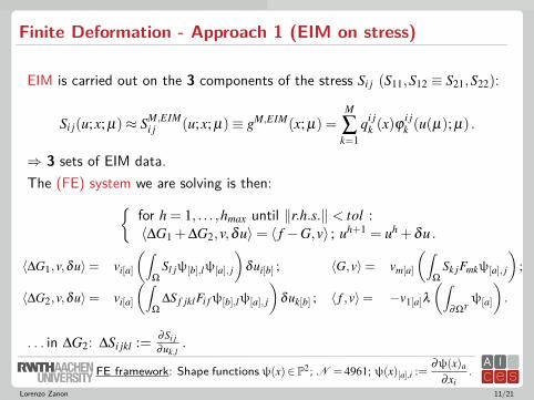
Finite Deformation - Approach 1 (EIM on stress)
EIM is carried out on the 3 components of the stress Si j (S11,S12 ≡ S21,S22):
Si j(u;x; µ)≈ SM,EIMi j (u;x; µ)≡ gM,EIM(x; µ) =
M
∑k=1
qi jk (x)ϕ
i jk (u(µ); µ) .
⇒ 3 sets of EIM data.The (FE) system we are solving is then:
for h = 1, . . . ,hmax until ‖r.h.s.‖ < tol :〈∆G1 +∆G2,v,δu〉= 〈 f −G,v〉 ; uh+1 = uh +δu .
〈∆G1,v,δu〉= vi[a]
(∫Ω
Sl jψ[b],lψ[a], j
)δui[b] ;
〈∆G2,v,δu〉= vi[a]
(∫Ω
∆S f jklFi fψ[b],lψ[a], j
)δuk[b] ;
〈G,v〉= vm[a]
(∫Ω
Sk jFmkψ[a], j
);
〈 f ,v〉= −v1[a]λ
(∫∂ΩT
ψ[a]
).
. . . in ∆G2: ∆Si jkl := ∂Si j∂uk,l
.
Lorenzo Zanon 11/21
FE framework: Shape functions ψ(x)∈P2; N = 4961; ψ(x)[a],i :=∂ψ(x)a
∂xi.

Finite Deformation - Approach 1 - EIM resultsEIM-Greedy on D train = µ = (E×ν)i, i = 1, . . . ,100 produces:
I Relative erroron the 3 stress components:
maxµ∈D train
‖SFEi j (µ)−SM,EIM
i j (µ)‖L∞,rel
M = 1, . . . ,Mmax; i j = 11,12,22.EIM dim. M
0 5 10 15 20 25
rel e
rro
r L
inf
10-8
10-7
10-6
10-5
10-4
10-3
10-2
10-1
100
EIM error Mmax=25
S11
S12
S22
I Interpolation points x∗mdistributed inside the domain:
Si j(u(x∗m; µ); µ) = SM,EIMi j (x∗m; µ);
m = 1, . . . ,Mmax; i j = 11,12,22.
0 0.2 0.4 0.6 0.8 10
0.02
0.04
0.06
0.08
0.1
0.12
0.14
0.16
0.18
0.2
S11
S12
S22
Lorenzo Zanon 12/21

Finite Deformation - Approach 1 - RB results
The RB-Greedy procedure, for M = 25:
for N = 1, . . . ,Nmax or ∆uRB−EIM < tolFor every µ ∈D train, find uRB−EIM
N :〈∆GRB−EIM
1 +∆GRB2 ,vRB
N ,δuRBN 〉= 〈 f RB−GRB,vRB
N 〉 , ∀vRBN ∈ ZRB
N ;
µ∗ = arg maxµ∈D train
∆uRB−EIM(N,µ) ; ZRBN+1 = ZRB
N ∪ζN+1 .
. . . introduces a relative error:
∆uRB−EIM(N,µ) := ‖uFE(µ)−uRB−EIMN (µ)‖rel
H1
I EIM applied only on ∆G1!I RB without EIM converges
almost 3 times faster;I No significant computational gain
with partial or pure RB!RB dim. N
2 5 8 11 14 17 20
Rel. E
rror
10-9
10-8
10-7
10-6
10-5
10-4
10-3
10-2
10-1
100
maxµ ∆ u
RB
maxµ ∆ u
RB-EIM
Lorenzo Zanon 13/21

Finite Deformation - Approach 1 - RB results
What error do we get from the EIM approximation of jacobian and residual?
Fixing M = Mmax:
maxµ∈D train
errG(N,µ) = ‖GRB(uRB
N (µ))−GRB−EIM(uRBN (µ))‖l1,rel ;
err∆G1(N,µ) = ‖∆GRB1 (uRB
N (µ))−∆GRB−EIM1 (uRB
N (µ))‖l1,rel ;
I The component ∆GRB−EIM1 is the
best-approximated . . .I . . . and can be utilized in the
RB-EIM-solve;I ∆GRB−EIM
2 (not in pic.), GRB−EIM arenot approximated well enough.
I Try a different approach . . .RB dim. N
2 5 8 11 14 17 20
Rel. E
rror
10-3
10-2
10-1
100
101
errG(N)
err∆G1(N)
Lorenzo Zanon 14/21

Finite Deformation - Approach 2 (EIM on (FS)nl)
EIM is carried out on the 4 components of the nonlinear part of (FS):
(FS)i j(x; µ) = (FS)lini j +(FS)nl
i j ≡ (FS)lini j +g(x;u; µ) :
(FS)lini j = (FS(u))lin
i j = (FS)linik uk, j(x; µ) ⇒ C×∇u
(FS)nli j = (FS(u))nl
i jEIM≈
M
∑k=1
qi jk (x)ϕ
i jk (u(µ); µ) ⇒ EIM approx.
⇒ 4 sets of EIM data.The (FE) system we are solving is then:
for h = 1, . . . ,hmax until ‖r.h.s.‖ < tol :〈∆Glin +∆Gnl ,v,δu〉= 〈 f −Glin−Gnl ,v〉 ; uh+1 = uh +δu .
〈∆Glin,v,δu〉= vi[a]
(∫Ω
∆(FS)lini jhkψ[b],kψ[a], j
)δuh[b] ;
〈∆Gnl ,v,δu〉= vi[a]
(∫Ω
∆(FS)nli jhkψ[b],kψ[a], j
)δuh[b] ;
〈Glin,v〉= vi[a]
(∫Ω
(FS)lini j ψ[a], j
);
〈Gnl ,v〉= vi[a]
(∫Ω
(FS)nli jψ[a], j
).
Lorenzo Zanon 15/21
A. Radermacher, POD-based model reduction in nonlinear solid mechan-ics. PhD thesis, RWTH Aachen University, 2014.

Finite Deformation - Approach 2 - EIM results
We can show that: ∆Gnl =∫
Ω
∆(FS)nli jhkψ[b],kψ[a], j
. . . is symmetric in both FE and EIM approximation⇔ the EIM data are independent of the component i j:
(FS)nl,M,EIMi j =
M
∑k=1
qAi jk (x)ϕA
i jk (u(µ); µ) .
maxi j=1,...,4
maxµ∈D train
‖(FS)nl,FEi j (µ)− (FS)nl,M,EIM
i j (µ)‖relL∞
I Convergence: ∼ 1.5 slower;I One set of EIM data;I About the same computational effort.
EIM dim. M0 10 20 30 40 50 60
Re
l. E
rro
r L
inf
10-14
10-12
10-10
10-8
10-6
10-4
10-2
100EIM error M
max=60
FS11
FS12
FS21
FS22
FSglob
Lorenzo Zanon 16/21

Finite Deformation - Approach 2 - RB results
The RB-Greedy procedure:
for N = 1, . . . ,Nmax or ∆uRB < tolFor every µ ∈D train, find uRB
N :〈∆GRB
lin +∆GRBnl ,v
RBN ,δuRB
N 〉= 〈 f RB−GRBlin −GRB
nl ,vRBN 〉 , ∀vRB
N ∈ ZRBN ;
µ∗ = arg maxµ∈D train
∆uRB(N,µ) ; ZRBN+1 = ZRB
N ∪ζN+1 .
. . . introduces a relative error:
∆uRB(N,µ) := ‖uFE(µ)−uRBN (µ)‖rel
H1 −→
I Pure RB convergence;I Without EIM still no computational gain!
RB dim. N
2 3 4 5 6 7 8 9 10 11 12 13
Rel. E
rror
H1
10-7
10-6
10-5
10-4
10-3
10-2
10-1
100
meanµ ∆ u
RB
maxµ ∆ u
RB
Lorenzo Zanon 17/21

Finite Deformation - Approach 2 - RB resultsWhat error do we get from the EIM approximation of jacobian and residual?
The error as a function of N and M:
maxµ∈D train
errGnl (N,M,µ) = ‖GRB
nl (uRBN (µ))−GRB−EIM,M
nl (uRBN (µ))‖l1,rel ;
err∆Gnl (N,M,µ) = ‖∆GRBnl (u
RBN (µ))−∆GRB−EIM,M
nl (uRBN (µ))‖l1,rel .
RB dim. N2 4 6 8 10
Rel. E
rror
l1
10-5
10-4
10-3
10-2 Error on the Residual
M = 10M = 20M = 30M = 40M = 50M = 60
maxµ errG
nl(N,M,µ)
RB dim. N2 4 6 8 10
Rel. E
rror
l1
10-4
10-3
10-2
10-1
100
101 Error on the Jacobian
M = 10M = 20M = 30M = 40M = 50M = 60
maxµ err∆ G
nl(N,M,µ)
With this approach, for M sufficiently large, we can approximateboth residual and jacobian . . .
Lorenzo Zanon 18/21

Finite Deformation - Approach 2 - RB resultsWhat error do we get from the EIM approximation of jacobian and residual?
For a fixed M = M∗ (min-max for best-performance):
maxµ∈D train
errGnl (N,M∗,µ) = ‖GRB
nl (uRBN (µ))−GRB−EIM,M∗
nl (uRBN (µ))‖l1,rel ;
err∆Gnl (N,M∗,µ) = ‖∆GRBnl (u
RBN (µ))−∆GRB−EIM,M∗
nl (uRBN (µ))‖l1,rel .
I The error on ∆Gnl is 1-3 o.o.m. biggerthan that on Gnl . . .
I . . . and increases with N!I Such an approximation of ∆Gnl
probably still not sufficient for anEIM-RB solve!
I Improvement w.r.t Approach 1.RB dim. N
2 4 6 8 10
Rel. E
rror
l1
10-5
10-4
10-3
10-2
10-1Error on Jacobian and Residual for best M
* = 50
maxµ err∆ G
nl(N,M*,µ)
maxµ errG
nl(N,M*,µ)
Lorenzo Zanon 19/21

Outline
1. Motivation2. The Reduced Basis Method3. Fundamental Equations in Elasticity4. Numerical Example: Finite Deformation5. Conclusion
Lorenzo Zanon

Part 5 - Summary and future work
We discussed:I overview of the RB Method;I application of the RB Method to finite deformation in elasticity.
Current and future work include:I further investigation on the RB-EIM finite deformation problem;I deriving error estimates for the RB approximation
in the finite deformation framework;I implementing the RB-EIM model for other hyperelastic laws (Neo-Hooke).
Lorenzo Zanon 20/21
Philippe G. Ciarlet, Mathematical Elasticity. Volume 1: Three Dimen-sional Elasticity. Elsevier, 2004.

Acknowledgements to:
I Karen Veroy-Grepl, Martin Grepl and RB team at AICES-RWTH Aachen;I Annika Radermacher and Stefanie Reese at IFAM-RWTH Aachen;I Garrett Christians (UROP Int. Project 2014);I David Knezevic and the libMesh support team.
Financial support from theDeutsche Forschungsgemeinschaft
through grant GSC 111is gratefully acknowledged
Lorenzo Zanon 21/21

Part 4 - Buckling Example - FE Eigenmodes
Physical eigenmodes resulting from a FE simulation on a column . . .
ξ1,2,3(µ) for a 2D column ξ1,2,3,4(µ) for a 3D column
Only the first eigenvalue λ1(µ) is the object of the RB approximation!
Lorenzo Zanon 22/21
L. Zanon and K. Veroy-Grepl. The reduced-basis method for an elasticbuckling problem. PAMM Proceedings, 2013.

Buckling Example - Truss Structure
. . . or a simple 2D truss structure.I Need to change the b.c., not the formulation;I Subdivision into 4 subdomains, more challenging affine decomposition;I In the online phase, RB allows for quick optimization.
Two-dim. parameter case:
t ≡ µ ∈D = [0.03125×0.2]2
H = 1m, mesh size = 0.02;
#D train = 17×17
#Donline = 18×18
Lorenzo Zanon 23/21
X. Guo, G. Cheng, K. Yamazaki, A new approach for the solution of singular optima in truss topology optimization
with stress and local buckling constraints. Struct. Multidisc. Optim. 2001.
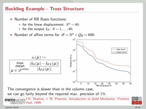
Buckling Example - Truss Structure
I Number of RB Basis functions:I for the linear displacement: Nu = 40;I for the output λN : N = 1, . . . ,40;
I Number of affine terms for B = Nu×QB = 600.
er(µ) :=max
meanµ ∈Donline
|λN(µ)−λFE(µ)||λFE(µ)|
5 10 15 20 25 30 35 4010
−6
10−4
10−2
100
102
RB Dimension N
Rela
tive E
rror
max error
mean error
The convergence is slower than in the column case,we can go fairly beyond the required max. precision of 1%.
Lorenzo Zanon 24/21
I.H. Shames, J. M. Pitarresi, Introduction to Solid Mechanics. PrenticeHall, 1999.

Buckling Example - Truss Structure
CPU Ratio FE vs. RB for the Eigenvalue Problem:
#Donline = 18×18
Nmax = 40
CPU ratio(N) =maxDonline tN(µ)maxDonline tFE(µ)
,
∀N = 1, . . . ,Nmax.
0 10 20 30 400
0.5
1
1.5
2
2.5
3
RB Dimension N
ma
x C
PU
ra
tio
(%
)
Extension to a 3D structure ⇒ More substantial computational gain.
Lorenzo Zanon 25/21
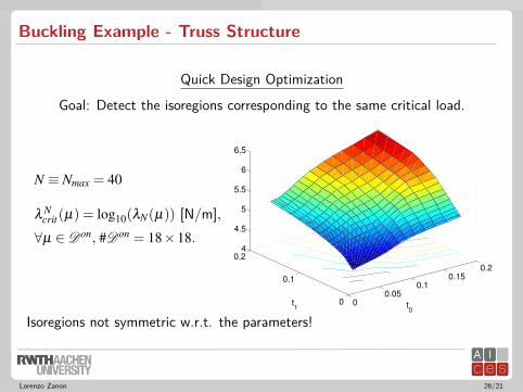
Buckling Example - Truss Structure
Quick Design Optimization
Goal: Detect the isoregions corresponding to the same critical load.
N ≡ Nmax = 40
λ Ncrit(µ) = log10(λN(µ)) [N/m],∀µ ∈Don, #Don = 18×18.
0
0.05
0.1
0.15
0.2
0
0.1
0.2
4
4.5
5
5.5
6
6.5
t0
t1
Isoregions not symmetric w.r.t. the parameters!
Lorenzo Zanon 26/21