On the Small and Finite Deformation Thermo-elasto...

European Journal of Computational Mechanics. Volume 15 – no 7-8/2006, pages 945 to 987

On the Small and Finite Deformation Thermo-elasto-viscoplasticity Theory for Strain Localization Problems: Algorithmic and Computational Aspects G. Z. Voyiadjis* — R. K. Abu Al-Rub* — A. N. Palazotto** * Department of Civil and Environmental Engineering, Louisiana State University, Baton Rouge, Louisiana 70803, USA [email protected] [email protected] ** Department of Aeronautics and Astronautics, Air Force Institute of Technology, WPAFB, OH 45433-7765, USA [email protected]

ABSTRACT. This work is focused on the numerical implementation of thermo-viscoplastic constitutive equations in small and finite strain contexts using FEM. A length scale parameter is introduced implicitly through viscosity in order to address strain localization in the (initial) boundary value problems. The mathematical structure of the infinitesimal viscoplasticity theory is concise and similar to that of the finite strain theory. These characteristics make the numerical implementation of this theory easy. The proposed numerical algorithms are implemented in such a way that the extension from the standard small strain FEM code to the finite strain analysis is straightforward. An extension to the viscoplastic range of the classical radial return algorithm for plasticity is developed. Numerical examples prove the excellent performance of the present framework in describing the strain localization problem.

KEYWORDS: Viscoplasticity; Finite Strain; Localization; Isotropic-Kinematic Hardening.

1. Introduction

Experimental observations of the plastic behavior of various materials reveal the existence of localization phenomena. This phenomenon is observed on a wide class of engineering materials including metals, concrete, rock, and soil, and is a characteristic feature of inelastic deformations. Strain localization is a notion describing a deformation mode, in which the whole deformation of a material structure occurs in one or more narrow bands, while the rest of the structure usually exhibits unloading. The width and direction of localization bands depend on the

946 European Journal of Computational Mechanics. Volume 15 – no 7-8/2006

material parameters, geometry, boundary conditions, loading distribution, and loading rate.

The strain localization behavior cannot be characterized using the classical inelasticity theory as it does not incorporate material length scales and consequently it cannot predict mesh-insensitivities. However, the developed elasto-viscoinelasticity theory (Perzyna, 1966) can be used for this purpose. Rate dependency (viscosity) allows the spatial difference operator in the governing equations to retain its ellipticity and the initial value problem (the Cauchy problem) is well-posed. Viscosity introduces implicitly a length-scale parameter into the dynamic initial-boundary value problem (e.g. Duszek-Perzyna and Perzyna, 1998; Dornowski and Perzyna, 2000), such that: vpcλ η= [1] where /c E ρ= denotes the velocity of the propagation of the elastic waves in the material, E is the Young’s modulus, ρ is the mass density, and vpη is the relaxation time for the mechanical disturbances which is directly related to the viscosity of the material. The proportionality factor λ depends on the particular initial-boundary value problem under consideration and may also depend on the microscopic properties of the material. Sluys (1992) has also demonstrated that this viscous length scale effect can be related to the spatial attenuation of waves that have real wave speeds in the softening regime.

Consequently, any rate dependence in the constitutive law combined with inertial effects introduces a length scale. This effect gives the possibility to obtain mesh-insensitive results (e.g. Needleman, 1988; Loret and Prevost, 1990; Prevost and Loret, 1990; Sluys, 1992; Wang et al., 1996, 1997, 1998; Duzek-Perzyna and Perzyna, 1998; Wang and Sluys, 2000; Dornowski and Perzyna, 2000, Glema et al., 2000). The rate-independent inelastic response is obtained as a limit case when the relaxation time is equal to zero, i.e. 0vpη = ; hence, the theory of viscoinelasticity offers the localization limiter (or regularization procedure) for the solution of dynamic initial-boundary value problems under different type of loadings. Furthermore, the size of the localized zones in which high strain gradients prevail and strain accumulation take place, is proportional to the length scale parameter , which is the distance the elastic wave travels in the characteristic time vpη (Sluys, 1992). Viscosity can thus be considered either as a regularization parameter (computational point of view), or as a micromechanical parameter to be determined from observed shear-band widths (physical point of view).

The purpose of this study is to demonstrate the regularization nature and significance of the viscoplasticity assumption in initial boundary value problems as a localization limiter, i.e. as means of preserving the well-posedness and discretization sensitivity in (initial) boundary value problems for strain softening media. Of particular interest are ill-posed (initial) boundary value problems in

Small and Finite Deformation Thermo-viscoplasticity for Strain Localization 947

elasto-viscoinelastic solids that lack solutions with continuous displacements. Therefore, attention is focused on materials with negative (strain softening) hardenings. However, it is imperative to emphasize that for multidimensional constitutive descriptions of plastic flow, finite deformation, strain softening and/or perfect plasticity/damage models are neither necessary nor sufficient for ill-posedness (Wang and Sluys, 2000).

It is worth to mention that there are several other approaches that can be used to preserve the well-posedness of the governing equations of the softening media. These approaches explicitly introduce material length scales into the constitutive equations. For example, non-local theory (Pijaudier-Cabot and Bazant, 1987; Bazant and Pijaudier-Cabot, 1988) and gradient-dependent theory (Aifantis, 1984) were used as localization limiters by many researchers (e.g. de Borst and Mühlhaus, 1992; de Borst and Pamin, 1996; Wang et al., 1998; Ramaswamy and Aravas, 1998a,b; Geers et al., 2000; Nedjar, 2001; Jirásek and Rolshoven, 2003; Voyiadjis et al., 2003, 2004; Abu Al-Rub and Voyiadjis, 2005). For a comprehensive review of these approaches consult Abu Al-Rub (2004). These approaches can be easily adapted to the proposed model, but the matter is beyond the scopes and the limits of the present paper (see e.g. Voyiadjis et al., 2003, 2004).

Unified update algorithms for thermo-elasto-viscoplastic constitutive equations for metals subjected to small or large deformations are developed. These constitutive equations were mathematically formulated based on the thermodynamic principles by Voyiadjis et al. (2004). Isotropic and kinematic hardenings are included in the constitutive frame. This paper focuses on the numerical part of these equations. Several computational frameworks are presented here for small-strain thermo-elasto-viscoplasticity and their direct and simple extension to finite deformations. The proposed unified integration algorithms are extensions of the classical rate-independent radial return scheme to the rate-dependent problems. Therefore, the same algorithms are able to integrate both elasto-plastic and elasto-viscoplastic models. These algorithms are very inexpensive and continuum and consistent tangent moduli can be obtained in closed forms. Furthermore, a trivially incrementally objective integration scheme is established for the rate constitutive relations. The proposed finite deformation scheme is based on hypoelastic stress-strain representations and the proposed elastic predictor/viscoplastic corrector algorithm allows for total uncoupling of geometrical and material nonlinearities. It is based on a geometrically, incrementally objective, elastic predictor, followed by a return mapping algorithm, on a frozen configuration that is totally identical to the return algorithm of the equivalent constitutive model in the small strain framework. As in the small strain model the total rate of deformation is viewed as the sum of the elastic and of the viscoplastic parts. The attributes that we strive for in this work are obtaining mesh objective results and ease of computer implementation. This computational framework has been implemented in ABAQUS and it has been used to simulate strain localization and material instability problems.

Along these lines, some authors were successful in achieving some of the above desirable objectives. See for example the works of Wang and Sluys (2000), Chaboche and Cailletaud (1996), Carosio et al. (2000), Heeres et al. (2002), Ponthot


(2002), Khoei et al. (2003), Lubarda et al. (2003), Lin and Brocks (2004), and Gomaa et al. (2004). Although all of the finite strain/viscoplastic laws proposed in these works can reduce automatically to the corresponding infinitesimal/plastic theories at small deformations and small strain rates, most of them have complicated mathematical forms and are not direct analogies of the small deformation and rate-independent theories. The complicated mathematical structures usually cause complicated procedures in numerical implementation. In this paper we are trying to overcome some of these numerical difficulties.

The outline of this paper is as follows: in Section 2 the recently proposed constitutive equations by Voyiadjis et al. (2004) for thermo-elasto-viscoplastic materials are recalled. Rate-dependent consistency condition is proposed for dynamic related problems in Section 3. The computational algorithms for implementing such an approach in the well-known finite element code ABAQUS (2003) are discussed thoroughly in this section. Closed form expressions for the continuum and consistent elasto-viscoplastic moduli are derived in Section 4. In Section 5, the extension of a small deformation material model to finite deformation problems is discussed. The updated Lagrangian formulation is adopted in the formulation of the kinematics. In Section 6, numerical examples of localization behavior are presented in order to show the validity of the proposed viscoplastic consistency and finite strain approaches.

2. Constitutive Equations

In this section, we outline a summary of the thermodynamically derived constitutive equations by Voyiadjis et al. (2004) neglecting the damage effect and the strain gradient effect. The following set of constitutive equations for thermo-elasto-viscoplastic continuum, will be integrated numerically in the subsequent sections.

Adapting the standard additive decomposition of strain rates ε into an elastic part eε and a plastic part pε , the stress rate can be written as ( ): vp= −σ ε εE [2] where ( ): stands for tensor contraction and E is the fourth-order elasticity tensor, which is temperature independent and can be given as ( )2 / 3ijkl ij kl ik jl ij klE K Gδ δ δ δ δ δ= + − [3] where K is the bulk-modulus, G is the shear-modulus, and δ is the Kronecker delta. The mechanical strain ε is equal to the total strain minus the thermal strain. The dynamic yield surface, f , is expressed as follows ( ) ( ) ( )3 1

2 : 1 ( ) ][1 ] 0[ ][ nvp myp mf R p T Tσ η= − − − + + − ≤τ τX X [4]


where τ is the deviatoric component of the Cauchy stress tensor σ (i.e.

13ij ij ij kkτ σ δ σ= − ), X is the back-stress tensor or the kinematic hardening

conjugate force, ypσ is the initial yield stress at the reference temperature oT T= ,

R is the isotropic hardening conjugate force, vpη is the viscoplasticity relaxation

time, 2 : / 3vp vpp = ε ε is the effective plastic strain, m is the strain-rate hardening exponent, mT is the melting temperature, and n is the temperature-softening exponent.

This criterion is a generalization of the classical von-Mises yield criterion of rate-independent materials to rate-dependent materials. The former can be simply recovered by imposing 0vpη = (no viscosity effect), so that one has the plasticity case 0f ≤ . Therefore, the admissible stress states are constrained to remain on or within the elastic domain, so that one has similar to rate-independent plasticity

0f ≤ . However, during the unloading process for rate dependent behavior, 0f < and for a particular strain-rate does not imply that the material is in the elastic domain, but it may also be in a viscoplastic state with a smaller strain-rate. The extended criterion given by Eq. [4] will play a crucial rule in the dynamic finite element formulation described hereafter. It also allows a generalization of the standard Kuhn-Tucker loading/unloading conditions: 0f ≤ , 0vpλ ≥ , 0vp fλ = , 0vp fλ = [5] where vpλ is the viscoplastic multiplier. The dynamic yield surface f can expand and shrink not only by softening or hardening effects, but also due to softening/hardening rate effects. Moreover, the right-hand-side of f defines the flow stress as a function of strain, strain-rate, and temperature and it converges to a great extent to the constitutive laws of Johnson and Cook (1985), Zerilli and Armstrong (1987), and Voyiadjis and Abed (2005).

It should be mentioned that the proposed rate- and temperature-dependent yield condition, Eq. [4], has a consistency condition (Kuhn-Tucker loading/unloading condition, Eq. [5]). This means that the stress remains on the yield surface, which is different from the well-known overstress laws of Perzyna (1966) and Duvant-Lions (1972). The proposed model has the advantage in comparison with the overstress models that it can be easily implemented in the classical rate-independent plasticity.

The kinematic hardening rule, X , that appears in Eq. [4] can be expressed using the Chaboche and Rousselier (1983) series, which was thermodynamically derived by Chaboche (1991), such that ( )

1

M kk =

= ∑X X [6]


where M being the number of desired kinematic hardening components, where each component is made to evolve independently using the Armstrong and Frederick (1966) rule and is given by 2( ) ( ) ( ) ( )

3k k vp k kC pγ= −εX X [7]

A more general kinematic hardening rule was derived thermodynamically by Voyiadjis and Abu Al-Rub (2003) in which Eq. (4) is a special case of that rule. The material constants ( )kC and ( )kγ ( 1, 2,...,k M= ), which can be identified based on the stress-strain data obtained from the half cycle of the uniaxial tension or compression experiments (Voyiadjis and Abu Al-Rub, 2003). The isotropic hardening rule, R, appears in Eq. [4] is evolved as follows [ ]R b Q R p= − [8] where b and Q are material constants. Eq. [8] was proposed by Chaboche (1991) and thermodynamically derived by Voyiadjis and Abu Al-Rub (2003) and coupled to damage evolution by Voyiadjis et al. (2003).

A local increase in temperature may influence the material behavior during deformation, which demands the inclusion of temperature in the constitutive modeling of the material. The thermomechanical heat balance equation for adiabatic conditions is expressed as follows: : :vp

pc T Rpρ = ϒ − −σ ε αX [9] where ρ is the material density, pc is the specific heat at constant pressure, ϒ is

the fraction of the viscoinelastic work rate converted to heat, and vp fλ= ∂ ∂α X is the flux variable associated with the kinematic hardening. We adapt an associated flow rule for the evolution of the viscoplastic strain as vp vpλ=ε N [10] where f= ∂ ∂σN is the gradient to the yield surface f , and is given by ( )3 2 /= − −τ τN X X [11] The evolution law in Eq. [8] can be used as an isotropic hardening law or isotropic softening law if the Q parameter, which characterizes the hardening/softening saturation level, is expressed as follows (Chaboche, 1991): ( ) ( )expM o MQ Q Q Q qp= + − − [12]


where MQ , oQ , and q are material constants. Figure 1 shows how Eq. [8] with the aid of the above expression can be used as a hardening or softening law. Therefore, the evolution of the state variable R allows the modeling of cyclic hardening or softening behavior.

3. Time Integration Procedure

In this section a new implicit stress integration algorithm is proposed based on the radial return method and backward Euler integration. The radial return in now extensively used in finite element codes for large-scale computations of elasto-plastic behavior (see Simo and Hughes (1998) and Belytschko et al. (2000) for a review of the many works that used this method). This integration algorithm is inexpensive and accurate. In addition, it allows the writing down of a closed-form expression for the consistent (algorithmic) tangent modulus. Use of this consistent modulus (and not the continuum modulus) for the establishment of the global tangent stiffness matrix is essential in preserving the quadratic rate of convergence in Newton-Raphson’s procedure required by implicit algorithms. In the following, we will extend the radial return algorithm of thermo-elasto-plasticity to thermo-elasto-viscoplasticity. This stress update algorithm treats the elasto-plastic and elasto-viscoplastic problem in a unified way. The algorithm is unified in a sense that the same routines are able to integrate both thermo-elasto-plastic and thermo-elasto-viscoplastic models by simply setting the viscosity parameter, vpη , to zero. Another unified approach was proposed by Chaboche and Cailletaud (1996) for integrating plasticity and viscoplasticity models.

(a) (b)

Figure 1. Behavior of the work-hardening-softening law Eq. [8]. (a) 1( ) ( )expM o MQ Q Q Q qp= − + − − , 2 ( ) ( )expM o MQ Q Q Q qp= + − , 3 0Q = , 4

( ) ( )expM o MQ Q Q Q qp= + − − , (b) ( ) ( )expM o MQ Q Q Q qp= + − − .


For the interval from step n to 1n + , the backward Euler method enables the proposed constitutive model in Section 2 to be discretized as follows:

( )13 11 1 1 1 12 1 ( / ) ][1 / ] 0[ ][ nmvp

n n n yp n n mf R p t T Tσ η+ + + + += − − + + Δ Δ − ≡τ X [13] where the evolution equations of the isotropic hardening, kinematic hardening, temperature, and viscoplastic strain are given by: ( )

1 11

M kn nk+ +=

= ∑X X [14] 2( ) ( ) ( ) ( ) ( )

1 13k k k vp k k

n n nC pγ+ += + Δ − ΔεX X X [15] [ ]1 1n n nR R b Q R p+ += + − Δ [16] : :vp

p n n nc T R pρ Δ = ϒ Δ − Δ − Δσ ε αX [17] 1

vp vpnλ +Δ = Δε N [18]

( )3 21 1 1 1 1/n n n n n+ + + + += − −τ τN X X [19] For J2-flow theory we can simply set vpp λΔ = Δ . If the variables at time nt (i.e. step n ), such as nσ , nε , nX , ( )k

nX , nT , nR , etc., are assumed to have been determined and the values of Δε and tΔ are given, then 1n+σ that satisfies the discretized constitutive equations can be solved. In the following, an elastic predictor-plastic corrector method (radial return mapping algorithm) is used. However, here we will extend this method to the time-dependent case. In the first step, the elastic predictor problem is solved with initial conditions that are the converged values of the previous time step while keeping irreversible variables frozen. This produces a trial elastic stress state trσ which, if outside the yield surface f is taken as the initial conditions for the solution of the viscoplastic corrector problem. The scope of this second step is to restore the consistency condition by returning back the trial stress to the generalized yield surface f .

3.1. Return mapping algorithm: radial return method

3.1.1 Elastic predictor

The elastic predictor can be tentatively obtained by assuming the entire strain increment Δε as elastic, such that 1 :tr

n n+ = + Δσ σ εE [20] For this tentative stress state, the yield criterion is given by:


( )13 1

1 12 1 ( / ) ][1 / ] 0[ ][ nmtr tr vpn n n yp n n mf R p t T Tσ η+ += − − + + Δ Δ − ≡τ X [21]

where ( )1

1 1 13 trtr tr trn n nσ σ+ + += − 1τ with 1 is the second-order identity tensor. If

1 0trnf + ≤ , yielding does not occur in this step, and then 1

trn+σ is accepted as 1n+σ .

This means that the response is elastic and the trial stress and the state variables become the final stress and state variables.

3.1.2 Viscoplastic corrector

If 1 0trnf + > , 1

trn+σ cannot be accepted as 1n+σ due to yielding. Then 1n+σ can be

written using Eq. [20] as follows: ( )1 1 1 1: :vp tr vp

n n n n+ + + += − = − Δσ ε ε σ εE E [22] where : vpΔεE is the plastic corrector.

3.1.3 Smoothing of the stress state at yield point

If the initial yield surface has been crossed during the initial trial stress increment, then a smoothing step is necessary to find the stress state at the yielding point. This is shown schematically in Figure 2. If 1

cnσ + denotes the stress state at the

point where the assumed stress path comes into contact with the initial yield surface, then we can write 1

c trn n β+ = + Δσ σ σ ; 0 1β≤ ≤ [23]

where :trΔ = Δσ εE is the trial stress increment and trβΔσ is the portion of the stress increment necessary to bring the trial stress state to the initial yield surface. In this, βΔε is the proportion of the strain increment at which the viscoplastic behavior is first encountered (i.e. when 0f = is reached). Now the condition

1( , , , ) 0cn n n nf X R Tσ + = leads to a quadratic equation for the determination of β .

However, a simple approximate value of β can be obtained by a linear interpolation in f (Nayak and Zeinkiewicz, 1972), that is 1/( )o of f fβ = − − [24] where ( , , , ) 0o n n n nf f X R Tσ= < and 1 1( , , , ) 0tr

n n n nf f X R Tσ += > . Due to the nonlinearity in the function f , however, 1 2( , , , ) 0c

n n n nf X R T fσ + = ≠ and a small departure from the yield surface is obtained. A more accurate estimate can be obtained from


1 2 1 1( ) :tr tr

o o n nf f f fβ + += − − − ΔσN [25] The portion of the strain increment for elastoplastic deformation is given by (1 )β− Δε and is used as the new given strain increment. Thus, the remaining portion of the trial stress increment beyond the contact stress can be calculated as (1 ) :β− ΔεE . We can then proceed to the next step in the following algorithmic development.

3.1.4 Nonlinear scalar equation

It is seen from Eq. [22] that 1n+σ can be readily obtained if vpΔε is found. For isotropic elasticity, with additive decomposition of total strain and associated flow, the problem can be reduced to solving a nonlinear scalar equation. Therefore, such an equation for the proposed model is sought in the following paragraphs thanks to the first attempts by Simo (see Simo and Hughes, 1998). It should also be mentioned that such a simplification is only possible in the particular case of isotropic elasticity and isotropic viscoplastic constitutive equations. Its immediate generalization to anisotropy was given by Chaboche and Cailletaud (1996), where the minimum number of equations to be solved iteratively is 6 (5 components of the vpΔε and the increment vpλΔ ). It can be noted that the extension to viscoplasticity (as well as to evolution equations containing thermal recovery effects) of a similar return mapping algorithm, has been already given by Chaboche and Cailletaud (1996).

Since the deviatoric part of the second term on the right of Eq. [22] is equal to 2 vpGΔε due to the assumption of elastic isotropy and plastic incompressibility, then using Eq. [18] the deviatoric expression of Eq. [22] becomes

33σ

11σ22σ of

oσ1f

1σ

(Initial yield surface)

(Updated yield surface)

cσtrσ

:trΔ = ΔEσ ε

trβΔσ ( )1 trβ− Δσ

Correction δσ

Figure 2. Stress smoothing algorithm for an initially plastic point.


1 1 12tr vp

n n nG λ+ + += − Δτ τ N [26] Combining Eq. [26] with Eq. [14] gives ( )

1 1 1 1 112 Mtr vp k

n n n n nkG λ+ + + + +=

− = − Δ − ∑τ τX N X [27] Eqs. [15] and [16] can be rewritten with the aid of Eq. [18] and vpp λΔ = Δ as follows ( )2( ) ( ) ( ) ( )

1 1 13k k k k vp

n n n nA C λ+ + += + ΔX X N [28] ( )1 1

vpn n nR B R bQ λ+ += + Δ [29]

where

1( ) ( )1 1k k vp

nA γ λ−

+ ⎡ ⎤= + Δ⎣ ⎦ , 1

1 1 vpnB b λ

−

+ ⎡ ⎤= + Δ⎣ ⎦ [30] Substituting Eq. [28] into Eq. [27] yields ( )2( ) ( ) ( )

1 1 1 1 131 12M Mtr k k k vp

n n n n n nk kA G C λ+ + + + += =

− = − − + Δ∑ ∑τ τX X N [31] The following equality can be easily obtained ( )2

3− = −S X S X N [32]

With the aid of the above equality, we can rewrite Eq. [31] as follows:

( ) ( )2 21 1 1 1 1 113 3

Mtr k k trn n n n n n nk

A+ + + + + +=− = − ∑τ τX N X N [33]

( )2 ( ) ( )1 13 1

2 M k k vpn nk

G A C λ+ +=− + Δ∑ N

Taking the tenor product of this equation with 1n+N such that 1 1tr

n n+ +=N N and

1 1: 1.5n n+ + =N N , we can then write Eq. [33] as follows ( )( ) ( ) ( ) ( )3 3

1 1 1 1 11 12 23M Mtr k k k k vp

n n n n n nk kA G A C λ+ + + + += =

− = − − + Δ∑ ∑τ τX X [34] Now, using the yield condition at the end of the increment, Eq. [13], we obtain the following expression ( )( ) ( )

1 1 113 [ ]Mtr k k vp

n n yp nkY G A C Rλ σ+ + +=

− + Δ = +∑ [35]

( )1111 ( / ) ][1 / ][ nmvp vp

n mt T Tη λ ++ Δ Δ −× where ( ) ( )3

1 1 112

Mtr tr k kn n n nk

Y A+ + +== − ∑τ X . This is the key equation for the numerical

method. It represents an algorithmic consistency condition for the considered


internal state variables. The increment for the kinematic hardening flux in Eq. [17] can be written as follows:

( )( ) ( )

( )1 1

32

kM Mk vp k

nkk kX p

Cγα α ε

= =

⎛ ⎞Δ = Δ = Δ − Δ⎜ ⎟

⎝ ⎠∑ ∑ [36]

Substituting the above equation together with Eqs. [15] and [18] into Eq. [17] yields ( )

( )3 ( ) ( )

( )2 1: :

kM k k vp

p n n n n n nkkc T R

Cγρ λ

=

⎛ ⎞Δ = ϒ − − − Δ⎜ ⎟

⎝ ⎠∑τ X N X X [37]

The corresponding temperature at 1nt + can be written as 1

vpn n nT T Z λ+ = + Δ [38]

( )

( )3 ( ) ( )

( )2 1

1 : :k

M k kkk

p

Z Rc C

γρ =

⎛ ⎞= ϒ − − −⎜ ⎟

⎝ ⎠∑τ X N X X [39]

Substituting Eqs. [29] and [38] into Eq. [35], a nonlinear scalar equation for vpλΔ is obtained. This is given as ( ) ( )( ) ( )

1 1 113 [ ]Mtr k k vp vp

n n yp n nkW Y G A C B R bQλ σ λ+ + +=

= − + Δ − + + Δ∑ [40]

111 ( ) ][1 ] 0[nvpvp

mvp n

m

T Zt T

λλη⎛ ⎞+ ΔΔ

+ − ≡⎜ ⎟Δ ⎝ ⎠×

where both ( )1

knA + and 1nB + are functions of vpλΔ (see Eq. [30]). Eq. [40] can be

solved using a local Newton-Raphson method with one variable in each successive iteration. The iterative procedure to find the zero value of ( )vpW W λ= Δ is then based on the relation ( ) ( )1 /vp vp vp vp

i i i iW Wλ λ λ λ+ ′Δ = Δ − Δ Δ [41] where W ′ is the gradient with respect to vp

iλΔ and is given as ( )

( )( ) ( ) ( )1 1

11 13

tr kM Mk k vp kn n

nvp vpk k

Y AW G A C Cλ

λ λ+ +

+= =

∂ ∂′ = − + − Δ∂Δ ∂Δ∑ ∑ [42]

( ) 1111 1 ( / ) ][1 ][ ][

nvpmvp vp vpn n

n nvpm

B T ZR bQ B bQ t

Tλ

λ η λλ

++

⎛ ⎞∂ + Δ+ Δ + + Δ Δ − ⎜ ⎟∂Δ ⎝ ⎠

−

( )111

1 ( / ) [1 ][ ]nvp

mvp vp vp nyp n nvp

m

T Zt B R bQ

Tmλ

η λ σ λλ +

⎛ ⎞+ Δ− Δ Δ + + Δ − ⎜ ⎟Δ ⎝ ⎠

( ) 111 1 ( / ) ] 0[ ][

nvpmvp vp vpn

yp n nvpmn

T ZnZ B R bQ tTT Z

λσ λ η λ

λ +

⎛ ⎞+ Δ+ + + Δ + Δ Δ ≡⎜ ⎟+ Δ ⎝ ⎠


where ( )

( )3 ( ) ( ) ( )1 1

1 1 12 1 1: /

tr kM Mtr k k k trn n

n n n n nvp vpk k

Y AA Y

λ λ+ +

+ + += =

⎡ ⎤∂ ∂= − −⎢ ⎥∂Δ ∂Δ⎣ ⎦

∑ ∑τ X X [43] ( )

( ) 2( ) ( )1 1k

k k vpnvp

A γ γ λλ

−+∂= − + Δ

∂Δ, ( ) 21 1 vpn

vp

Bb b λ

λ−+∂

= − + Δ∂Δ

[44] The iterations are ended when a desired accuracy in the yield function 1nf TOL+ ≤ falls to within a prescribed error tolerance TOL . The convergence is guaranteed because W is a convex function of vpλΔ . See Figure 3 for a geometric interpretation of the elastic predictor/plastic corrector algorithm in the deviatoric stress space.

It should be noted that for integration points that have already yielded in the previous increment (iteration), that is 0β = , and during the local (within the material algorithm) or global (within the finite element method) Newton-Raphson

33τ

11τ22τ

nf

nY

nX

1nf +

1n+X

1nY +

nτ

1trn+τ

11n+τ

1in+τ

11

in++τ

1n+τ

trΔτ

ΔX

Figure 3. Conceptual representation of the Elastic predictor/ viscoplasticcorrector algorithm.


iterative process, if the yield function f falls below the effective yield stress Y at the end of the previous increment (iteration), then that point is assumed to have unloaded elastically.

To complete the algorithmic procedure discussed above, there only remains to be computed an explicit expression for the tangent stiffness in order to accelerate the convergence of the finite element solution. In the following we will derive expression for the continuum or elastoplastic tangent modulus to be used if small time steps are used. Furthermore, an expression for the consistent or algorithmic stiffness modulus will be derived to be used for large time steps. In case of large time steps, the consistent tangent modulus may differ significantly from the continuum elastoplastic tangent. Therefore, for finite values of the step time size tΔ , use of the consistent tangent modulus is essential to preserve the quadratic rate of asymptotic convergence that characterizes the Newton-Raphson method (Simo and Hughes, 1998). Moreover, for programmable purposes it is easier to implement the continuum tangent stiffness as compared to the consistent tangent stiffness where for more involved yield conditions some derivatives can be extremely hard to compute if one uses the consistent tangent stiffness. Therefore, for the convenience of the reader both tangent moduli are presented here.

4. Thermo-elasto-viscoplastic Tangent Stiffness Moduli

4.1 Continuum tangent stiffness modulus

In the following, the continuum or elastoplastic tangent stiffness 1epn+ = Δ Δσ εD

will be derived for the above constitutive equations. For clarity we omit the subscript 1n + from the increment of a state variables ( ) 1n+

Δ in the following development since all the increments are provided at time step 1nt t += . The consistency condition, fΔ , can be written as 0

n n n n

f f f f p ff R TR p t T

∂ ∂ ∂ ∂ Δ ∂Δ ≡ Δ + Δ + Δ + + Δ =

∂ ∂ ∂ ∂Δ Δ ∂σ

σX

X [45]

Substituting Δσ , ΔX , RΔ , and TΔ from Eqs. [22], [15], [16], and [38], respectively, into the consistency condition, we can obtain a closed form expression for the viscoplasticity multiplier vpλΔ as 2 : /vp G HλΔ = ΔεN [46] where H is the hardening modulus and is given by ( ) ( ) 13 :n n n n

n n

f f fH G C b Q R ZR t p T

γ ∂ ∂ ∂= + − − − − −

∂ Δ ∂Δ ∂X N [47]

where


11[1 ( ) ][1 ( ) ]mvp nyp m

f p T TR

σ η∂= − + −

∂ [48]

11

1

1 ( ) [ ][1 ( ) ]mvp nyp m

f p R T Tp m t p

η σ∂= − + −

∂Δ Δ [49]

11( ) [ ][1 ( ) ]mn vp

m ypf n T T R pT T

σ η∂= + +

∂ [50]

and ( )

1

M kk

C C=

= ∑ , ( ) ( ) ( )1

M k kk

γ γ=

= ∑X X . The elasto-plastic tangent stiffness, epD , is defined by the rate of Eq. [22] along with Eqs. [18] and [46] such that:

2

1 1 1(4 / )epn n nG H+ + += − ⊗D E N N [51]

where ⊗ represents the dyadic tensor product. Eq. [47] shows how the relaxation time does affect the tangent operator. From Eqs. [47]-[50], the classical continuum tangent operator for elasto-plasticity can easily be recovered by setting 0vpη = (no viscosity effect).

4.2 Consistent (algorithmic) tangent stiffness modulus

In the following, the consistent or algorithmic tangent stiffness 1 d dalg

n+ = Δ Δσ εD is derived for the above proposed constitutive model. Differentiating Eqs. [18] and [22] gives ( )d : d d vpΔ = Δ − Δσ ε εE [52] 1d d dvp vp vp

nλ λ+Δ = Δ + Δε N N [53] ( )1d : d dn+= Δ − ΔτN XΖ [54] ( )3 2 /= − ⊗ −Z I τN N X [55] and I is the fourth-order unit tensor. Differentiating Eq. [46] with the aid of Eq. [54] yields ( )( )1 1

2d : d d : : dvpn n

GH

λ + +Δ = Δ − Δ Δ − Δτ ε εX NΖ [56] If dΔτ and dΔX can be expressed in terms of dΔε , the consistent tangent modulus can be easily obtained according to Eqs. [52]-[56]. Taking the deviatoric part of Eq. [52] and noting : d 2 dvp vpGΔ = Δε εE and the deviatoric part of dΔε is

: dd ΔI ε , the following equation can be derived ( )d 2 : d dd vpGΔ = Δ − ΔIτ ε ε [57]


where 13

d = − ⊗I I 1 1 , represents the deviatoric operation of a tensor. The differential of Eqs. [14] and [15], respectively, gives ( )

k=1d dM k= ∑X X [58]

( )2 2( ) ( ) ( ) ( ) ( ) ( )

13 3d d dk k k k vp k k vpn nA C A C+= + Δ + Δε εX X [59]

From Eq. [30]2, the differentials of ( )kA are obtained as

( )( )d d

kk vp

vp

AA λλ

∂= Δ

∂Δ [60]

where ( )k vpA λ∂ ∂Δ is given by Eq. [44]. However, since ( ) ( )d dk k= ΔX X we can write Eq. [58] as * *d d dvp vp

n CλΔ = Δ + ΔεX X [61] ( )

( )2* ( ) ( )31

kM k k vp

n nvpk

A Cλ=

∂= + Δ

∂Δ∑ εX X , 2* ( ) ( )13 1

M k knk

C A C+== ∑ [62]

Substituting Eqs. [57] and [61] into Eq. [56] produces

( ) ( )*1 1 1d 2 : : : d 2 : : dvp d vp

n n nh G G Cλ + + +⎡ ⎤Δ = Δ + Δ − + Δ Δ⎣ ⎦Z I Zε ε ε εN [63]

1*12 : :n nh H G

−

+⎡ ⎤= + Δ⎣ ⎦Zε X [64] Substituting Eqs. [54], [57], and [61] into Eq. [53] gives ( )1

1 1d 2 : : dvpn nG −

+ +Δ = ΔPε εΠ [65] where ( ) ( ) ( )* *

1 1 1 1 12 2 : :vp vpn n n n n nG C Gh λ λ+ + + + +

⎡ ⎤= + + Δ ⊗ − Δ + Δ⎣ ⎦I Z Z Zε N XΠ [66] ( ) ( )*

1 1 1 1 12 : : :d vpn n n n n nh G λ+ + + + += Δ + ⊗ − ΔP Z I Zε N N X [67]

Substituting Eq. [65] into Eq. [52] gives ( )2 1

1 1d 4 : : dn nG −+ +

⎡ ⎤Δ = − Δ⎣ ⎦Pσ εE Π [68]

Finally, an expression for the consistent tangent stiffness d dalg = Δ Δσ εD is derived as ( )2 1

1 1 14 :algn n nG −

+ + += − PD E Π [69]

For convenience, a step-by-step description of the algorithm discussed in Sections 3 and 4 is illustrated in the flow diagram presented in Figure 4. It is


noteworthy that assuming the material constants ( E , C , γ , etc) are temperature dependent makes the hypoelastic stress-strain relation in Eq. [2] is a valid elastic equation and its discretization in Eq. [20] is consistent with the choice and the main equations will not change except additional terms corresponding to the derivative of the material constants as a function of T will appear in the expressions of viscoplastic multiplier vpλΔ and tangent operators epD and algD .

nσ , nε , vp

nε , nX , ( )knX , nT , nR ; known

1n+Δε , tΔ ; given

1trn+σ

1 0trnf + ≥ NO 0vpλΔ = , 1 1

trn n+ +=σ σ ;

end

YES

Compute W and W ′ and solve for 1vpiλ +Δ by Newton-

Raphson method.

51 10nf

−+ ≤

NO

YES

1n+τ , ( )1

kn+X , 1n+X , 1n+N , 1nT + , 1nR +

1vpn+Δε

Successive substitution

1n+σ , ( )1

kn+X , 1n+X , 1nT + , 1nR +

epD or algD ; end

Figure 4. Flow chart of stress integration algorithm combining the successivesubstitution with the Newton-Raphson method.


5. Direct Extension to Finite Strain Hypoelasto-viscoplasticity

For small deformation problems, it is assumed that the difference between the reference configuration and the subsequent configuration is negligible. In this case the selection of stress and strain measures is unique. But for large strain problems, this difference cannot be neglected. The rigid rotation and the objectivity of material must be carefully treated in the constitutive formulation. The selection of stress and strain measures is no longer unique and the material time derivatives of the spatial stresses and strains are not objective. All these facts make the mathematical formulation and numerical analysis of finite strain viscoplasticity troublesome. In this section, an objective stress update algorithm is proposed for finite hypoelasto-viscoplasticity. The proposed procedure is implemented in such a way that the extension from the standard small strain FE code to the finite strain FE analysis is straightforward. The additional computational cost only includes some geometrical manipulations. The efficiency of the presented algorithm relies crucially on the total uncoupling between material and geometrical nonlinearities.

5.1 A corotational formulation

One of the major challenges while integrating the constitutive equations in finite deformation context is to achieve the incremental objectivity, i.e. to maintain correct rotational transformation properties all along a finite time step. However, when we applied time discretization procedures to objective rate constitutive equations, usually the objectivity is achieved in the limit of vanishing small time steps. In order to overcome this problem, a procedure that has now become very popular is first to rewrite the constitutive equations in a corotational moving frame. This corotational frame can be generated in the following way. Given a skew-symmetric tensor,

= −Ω Ω , (e.g. ω , the spin tensor =Ω ω , T=Ω R R , or the relative spin tenor T= −Ω ω RR ), we may generate a group of rotations ρ , by solving

=ρ Ω ρ with ( )nt t= = 1ρ [70] Now it is possible to generate a change of frame from the fixed Cartesian reference axes to the corresponding rotating axes (corotational axes). The Cauchy stress tensor σ can then be transformed by ρ as ˆ T=σ ρ σ ρ [71] Differentiating the above equation with respect to time, we obtain ( )ˆ T T ∇= − + =σ ρ σ Ω σ σ Ω ρ ρ σ ρ [72] where ∇σ is a corotational objective rate of the Cauchy stress. We can also write the rate of the backstress as


( )ˆ T T ∇= − + =ρ Ω Ω ρ ρ ρX X X X X [73]

In literature many objective rates are introduced, such as: Jaumann, Truesdell, and Green-Naghdi rates. From Eq. [72] we can obtain the Jaumann rate if =Ω ω , the Truesdell rate if T= −Ω ω RR , and the Gree-Naghdi rate if T=Ω R R . Moreover, Eq. [72] indicates that a somewhat complicated expression as an objective derivative becomes a rather simple time derivative under the appropriate change of coordinates. This suggests that the entire theory and implementation will take on canonically simpler forms if transformed to the ρ -system. For more details on this change of coordinates, see for example Simo and Hughes (1998). In the new reference frame, the evolution equations take the simpler form ( )ˆ ˆ ˆˆ ˆˆ : :e vp= = −σ E d E d d [74] The constitutive equations in Section 2 can still be used for finite deformations if no distinction between d (rate-of-deformation tensor) and ε (rate of small strain tensor), while the scalar quantities remain unchanged. The rate-of-deformation tensor in the unrotated frame can then be written as ˆ T= ρ ρd d , ˆ T= ρ ρX X , ˆ T= ρ ρN N , ( )ˆ T T= =ρ ρ ρ ρE E E [75] In order to complete the hypoelasto-viscoplastic constitutive equations in the context of finite deformation, the equations to integrate in the corotational frame are simply reduced to ( )ˆ ˆˆ : vp= −σ E d d [76] Assuming that the variables of the model at step n and the incremental displacement field 1n n+Δ = −u x x at load step 1n + are known, the trial elastic stress for a constant E can then be given by 1

ˆˆ ˆ :trn n t+ = + Δσ σ E d [77]

or, in the Cartesian frame, we can write the trial stress as follows ( )1 1 1 1 1 1

ˆˆ :tr tr T T Tn n n n n n n n nt+ + + + + += = + Δσ ρ σ ρ ρ ρ σ ρ ρE d [78]

Using the polar decomposition =F RU , we can write ( )1 1 1

2ˆ T T T− −= = +ρ ρ ρ ρd d R UU U U R [79]

Eq. [78] can then be simplified in the following way. Let us assume that the reference configuration is the configuration at time nt t= (update Lagrangian formulation). This implies that


n = 1ρ [80] Moreover, let us assume that ( ) ( )t t=ρ R [81] which implies that Eq. [79] reduces to ( )1 1 1

2ˆ − −= +d UU U U [82]

The use of the midpoint rule results in ( )1 1

2 2

1 1 12

ˆn n

t − −

+ +Δ = Δ + Δd UU U U [83]

where ΔU and 1

2n+

U in the above relation are

1n n+Δ = −U U U , ( )1

2

112 n nn ++

= +U U U [84] We can then express the trial elastic stress, Eq. [78], as follows ( )1 1

2 2

1 1 11 1 12 :tr T

n n n nn n− −

+ + ++ +

⎛ ⎞= + Δ + Δ⎜ ⎟⎝ ⎠

σ σR E UU U U R [85] In Eq. [85] we need to calculate the inverse of U . However, a simpler expression for the trial stress, which can be easily implemented using VUMAT or UMAT user material subroutines in the ABAQUS finite element code, can be obtained by adapting the following assumptions. Le us assume the following exponential map of

( )tU , such that (Simo and Hughes, 1998): ( ) ( )exp /nt t t t= − Δ⎡ ⎤⎣ ⎦U C [86] where C is a constant tensor to be determined. Upon time differentiation of Eq. [86] we obtain ( ) ( )exp /nt t t t

t= − Δ⎡ ⎤⎣ ⎦Δ

CU C [87] Substituting the above equation into Eq. [82], yields ˆ / t= Δd C [88] The tensor C is simply determined using the following compatibility conditions:

– in the reference configuration ( ), ntX : ( ) ( )expnt = =0 1U – in the current configuration ( )1, nt +x : ( ) ( )1 1expn nt + +=U C

From these two conditions, rewriting ( )1 1n nt + +=U U , it results in that


( )1 12

1 1 1 1 12 2ln ln ln Tn n n n n+ + + + += = =C U U F F [89]

which implies that C is the (incremental) natural strain tensor between the reference configuration and the current one. Hence, the trial elastic stress tensor in Eq. [78] can be evaluated by the following simpler expression than that in Eq. [85], such that ( )1 1 1 1:tr T

n n n n n+ + + += +σ σR E C R [90] The final mapped stress is given in Eq. [92]. In the above procedure, it is essential to realize that:

– =F RU are incremental tensors; it can be seen from Eq. [83] and Eq. [89] that the proposed procedure is trivially incrementally objective. In the case of rigid body motion, 1n n+ =U U and ˆ = 0d or ln = 0U , thus the stress tensor will be updated exactly by the relation 1

Tn n+ =σ σR R , whatever the amplitude of the

rotation; – the rotation tensor R is directly and exactly computed from the polar

decomposition and not from the (approximate) numerical integration of the rate equation =ρ Ω ρ over the time interval , 1[ ]n nt t + ;

– in the proposed procedure, R only needs to be evaluated once per time step. This is different from the schemes proposed in Simo and Hughes (1998), where it needs to be evaluated twice per time step;

– all kinematic quantities are based on the deformation gradient F over the considered time step, a quantity that is readily available in a nonlinear finite element code like ABAQUS.

For more details about the computation of the rotation tensor R and the logarithmic tensor C the reader is referred to Simo (1992) and Mahnken (2000). Now if ( )1, , , 0tr

n n n nf R T+ ≤σ X , the process is clearly elastic and the trial stress is in fact the final state. On the other hand, if ( )1, , , 0tr

n n n nf R T+ >σ X , the Kuhn-Tucker loading/unloading conditions are violated by the trial stress which now lies outside the generalized viscoplastic yield surface. Consistency, as shown in Section 3, is restored by a generalization of the radial return algorithm to rate-dependent problems. The viscoplastic corrector problem may then be rephrased as (the objective rates reduce to a simple time derivative due to the fact that the global configuration is held fixed): 1 1: : 2vp vp vp

n nt Gλ λ+ +Δ = − Δ = −Δ = − Δσ E d E N N [91] such that the elastic-predictor/viscoplastic corrector step yields the final stress as 1 1 12tr vp

n n nG λ+ + += − Δσ σ N [92]


Utilizing the above procedure, we can use the computational algorithm in Sections 3 and 4 in the finite deformation context such that no distinction is made between the rate-of-deformation tensor and the rate of small strain tensor and that the trial elastic stress is calculated using Eq. [90] or Eq. [85]. Therefore, once Eq. [40] is solved for

vpλΔ we can update the current stress in Eq. [92] and the other thermodynamic conjugate forces. Therefore, it should be emphasized that, with the exception of the nonlinear kinematic term d , the discretized constitutive equations are identical to those presented in Sections 3 and 4 for its small strain counterparts. Thus, the above procedure provides a material-independent prescription for extending small-strain updates into finite deformation range within the framework of a hypoelastic formulation (i.e. within the framework of additive decomposition of the rate-of-deformation tensors).

5.2 Finite deformation elasto-viscoplastic tangent moduli

Use of the consistent modulus, as opposed to the continuum modulus, is imperative in preserving the asymptotic rate of quadratic convergence in the Newton-Raphson method for the global finite element problem. The proposed finite deformation scheme indicates that a somewhat complicated expression for an objective derivative becomes a rather simple time derivative under the appropriate change of coordinates. Therefore, the expressions for the continuum tangent modulus and the consistent tangent modulus derived in Sections 4.1 and 4.2, respectively, can be used as they are in the proposed finite deformation context. However, conceptually (see Figure 5) for a graphical illustration, the continuum tangent operator epD is given by :ep∇ =σ D d [93]

0limep t t t+Δ

Δ →

−=

Δσ σ

xD

x, t t t+ΔΔ = −x x x [94]

whereas the consistent (algorithmic) tangent operator algD is given by d : dalg∇ =σ D d [95]

( 1) ( )

0lim

i ialg t t t t

++Δ +Δ

Δ →

−=

Δσ σ

xD

x [96]

where i is the iteration number and ( 1) ( )i i

t t t t+

+Δ +ΔΔ = −x x x [97] where all the values appearing in the continuum tangent operator are taken from equilibrated configurations, which is generally not the case for the consistent tangent operator. Therefore, it should be emphasized again that, with the exception of the nonlinear kinematic term d , the continuum or consistent tangent elasto-viscoplastic


operators are identical to its small strain counterparts presented in Eqs. [51] and [69], respectively. Thus, the above procedure provides a material-independent prescription for extending small-strain updates into finite deformation range within the framework of a hypoelastic formulation.

6. Numerical Examples

In this section, some numerical examples are presented to verify the implementation of the proposed viscoplasticity constitutive model using the commercial finite element program ABAQUS (2003). The algorithmic model presented in the previous section is coded as a UMAT user material subroutine of

tσ

tx

t t+Δσt t+Δx

Δ x

0limep t t t+Δ

Δ →

−=

Δσ σ

xD

x

(a)

tσtx

t t+Δσt t+Δx

Δ x

(1)t t+Δσ

( )it t+Δσ

( 1)it t

++Δσ

(1)t t+Δx

( )it t+Δx

( 1)it t

++Δx

( 1) ( )

0lim

i ialg t t t t

++Δ +Δ

Δ →

−=

ΔxD

xσ σ

(b)

Figure 5. Continuum and consistent tangent operators. Configurationsrepresented by a solid line have a physical meaning, while dotted linesrepresent non equilibrated configurations that only have a numericalexistence. (a) Continuum tangent operator, (b) consistent tangent operator.


ABAQUS/Standard (2003) and as a VUMAT user material subroutine of ABAQUS/Explicit (2003). ABAQUS/Standard is used for static as well as steady state dynamic problems and it uses implicit integration algorithms; while, ABAQUS/Explicit is mainly used for high transient dynamic problems and it uses explicit integration algorithms. For information about the way to implement material models in ABAQUS/Standard or ABAQUS/Explicit consult the reference manuals of ABAQUS (2003).

6.1 Uniaxial tension

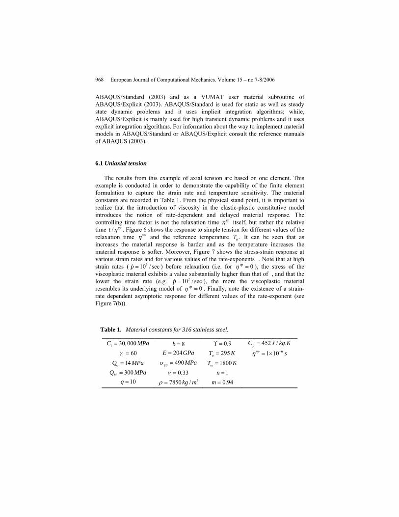
The results from this example of axial tension are based on one element. This example is conducted in order to demonstrate the capability of the finite element formulation to capture the strain rate and temperature sensitivity. The material constants are recorded in Table 1. From the physical stand point, it is important to realize that the introduction of viscosity in the elastic-plastic constitutive model introduces the notion of rate-dependent and delayed material response. The controlling time factor is not the relaxation time vpη itself, but rather the relative time / vpt η . Figure 6 shows the response to simple tension for different values of the relaxation time vpη and the reference temperature oT . It can be seen that as increases the material response is harder and as the temperature increases the material response is softer. Moreover, Figure 7 shows the stress-strain response at various strain rates and for various values of the rate-exponents . Note that at high strain rates ( 310 / secp = ) before relaxation (i.e. for 0vpη = ), the stress of the viscoplastic material exhibits a value substantially higher than that of , and that the lower the strain rate (e.g. 210 / secp = ), the more the viscoplastic material resembles its underlying model of 0vpη = . Finally, note the existence of a strain-rate dependent asymptotic response for different values of the rate-exponent (see Figure 7(b)).

Table 1. Material constants for 316 stainless steel.

1 30,000C MPa= 8b = 0.9ϒ = 452 / .pC J kg K=

1 60γ = 204E GPa= 295oT K= 61 10vp sη −= × 14oQ MPa= 490yp MPaσ = 1800mT K= 300MQ MPa= 0.33ν = 1n =

10q = 37850 /kg mρ = 0.94m =


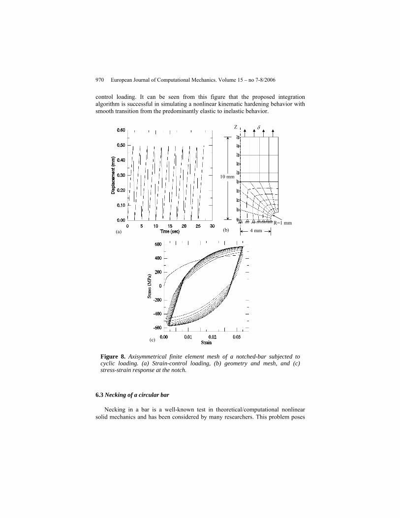
6.2 Cyclically loaded notched bar

This example is chosen to demonstrate the capabilities of the viscoplasticity kinematic hardening rule in simulation of cyclic loading and ratcheting. An axisymmetric notched bar subjected to uniaxial strain cycling with a non-zero mean strain is discussed (Figure 8(a)). The geometry and finite element mesh of the problem are shown in Figure 8(b), and a 2D axisymmetrical four-noded element mesh is employed. Due to symmetry a quarter of the notched bar is shown in Figure 8(b). Small deformation is assumed in this example. The material constants are listed in Table 1. Figure 8(c) shows the cyclic response at the notch due to a strain

vpη increases

vpη =0, 0.001, 0.005, 0.01 sec

T increases

T = 0, 300, 600, 900, 1200 K

(a) (b) Figure 6. Uniaxial tension behavior obtained (a) for increasing relaxation times

0,vpT η= = 0.001, 0.005, 0.01 sec, and (b) for increasing temperature 0T = ,300, 600, 900, 1200 K.

0secvpη =

310 / secp =

1 32 10 / secp =

210 / secp =

0.005secvpη =

(a)

m1 increases

m1 =2, 1, 0.5, 0.1

(b) Figure 7. Uniaxial stress-strain response (a) at various strain rates, and (b) atvarious strain-rate exponents.


control loading. It can be seen from this figure that the proposed integration algorithm is successful in simulating a nonlinear kinematic hardening behavior with smooth transition from the predominantly elastic to inelastic behavior.

6.3 Necking of a circular bar

Necking in a bar is a well-known test in theoretical/computational nonlinear solid mechanics and has been considered by many researchers. This problem poses

(a)

Z δ

10 mm

4 mm R=1 mm

(b)

(c)

Figure 8. Axisymmetrical finite element mesh of a notched-bar subjected tocyclic loading. (a) Strain-control loading, (b) geometry and mesh, and (c)stress-strain response at the notch.


the most severe test to a finite strain inelasticity formulation. Therefore, this problem is used to check the validity of the proposed finite strain approach. A circular bar, with a radius of 6.413mm and a length of 53.334mm, is subjected to uniaxial tension up to a total axial elongation of 10mm and a rate of loading of 0.2 m/s (Figure 9). For an ideal case of a perfect specimen, necking can start in any section of the specimen. In order to replace such a problem with multiple solutions by a problem with unique solution a geometric imperfection of 1% radius reduction is introduced to induce necking in the central part of the bar. The material parameters are listed in Table 2.

Table 2. Material properties for the necking of a circular bar.

1 193.8C MPa= 16.93b = 0.9ϒ = 452 / .pC J kg K=

1 0γ = 206.9E GPa= 0oT K= 0.0025vp sη = 265oQ MPa= 450yp MPaσ = 1800mT K=

0MQ MPa= 0.29ν = 1.0n = 0q = 37850 /kg mρ = 1.0m =

(b)

z

r

6.413 mm

6.350 mm

26.6

7 m

m

(a) Figure 9. Problem description of a necking of a circular bar. (a) The circularbar geometry, mesh, and boundary conditions. (b) Three dimensional shapecorresponding to quarter of the bar.


Four different meshes consisting of 50, 200, 400, and 800 four-noded elements with reduced integration, corresponding to one quarter of the specimen, are considered in order to assess the accuracy of the discretization [Figure 10(a)]. Their

(a)

(b) Figure 10. Necking of a circular bar. (a) Finite element meshes of 50, 200,400, and 800 elements, respectively. (b) Deformed patterns (the dashedlines represent the initial configuration).


corresponding initial and final deformed shapes are shown in Figure 10(b). The results in Figure 10(b) show that the proposed finite strain approach preserves the objectivity of the numerical results. Almost the same necking radius is observed for the four meshes. Figure 11 represents the history of the deformation for the 400 elements mesh corresponding to 2.5, 5, 7.5, and 10 mm of total elongation.

The contours of the effective plastic strain and the Cauchy stress components rrσ and zzσ for the four considered meshes are shown in Figures 12, 13, and 14,

respectively, after a total of 10 mm of axial elongation. It is shown that objective results are obtained for different meshes, which are almost independent of mesh refinement (i.e. minor mesh dependency is encountered).

In Figure 15(a) and 15(b) we examine the mesh sensitivity of the numerical results to subsequent mesh refinement. Figure 15(a) shows the ratio of the current radius ( R ) to the initial radius ( oR ) at the necking section versus the ratio of the axial elongation ( LΔ ) to the initial length ( L ) for the four meshes of 50, 200, 400, and 800 elements. Figure 15(b) shows the applied nominal stress versus the axial elongation. These figures corroborate the relative insensitivity of the numerical results to the mesh refinement.

Figure 11. Deformation history for the 400 elements mesh corresponding to 2.5,5, 7.5, and for 10 mm total elongation.


(a) (b)

(c) (d)

Figure 12. Contours of the effective viscoplastic strain for (a) 50 element mesh,(b) 200 element mesh, (c) 400 element mesh, and (d) 800 element mesh.


(a) (b)

(c) (d)

Figure 13. Contours of the Cauchy stress component in the radial direction rrσ(N/m2) of the (a) 50 element mesh, (b) 200 element mesh, (c) 400 element mesh,and (d) 800 element mesh.


(c) (d)

(a) (b)

Figure 14. Contours of the Cauchy stress component in the axial direction zzσ(N/m2) of the (a) 50 element mesh, (b) 200 element mesh, (c) 400 element mesh,and (d) 800 element mesh.


It is imperative to mention that with the use of the small strain algorithm, no global softening behavior is observed. With the contribution of geometrical nonlinearity, however, one observes the global softening at around 10% deformation, even though, locally, the material shows hardening behavior (see Figures 11 and 15). Moreover, the computation in this example is in the quasi-static range and, therefore, the viscosity only brings a characteristic time and no characteristic length.

0.75

0.8

0.85

0.9

0.95

1

0 0.05 0.1 0.15 0.2ΔL/Lo

R /

Ro

50 elements200 elements400 elements800 elements

(a)

50 elements

200, 400, 800 elements

0

500

1000

1500

0 2 4 6 8 10ΔL (mm)

Stre

ss (M

Pa)

50 elements200 elements400 elements800 elements

(b)

50 elements

200, 400, 800 elements

Figure 15. Necking of a circular bar. Numerical study of the sensitivity of thecalculation with respect to the mesh refinement. (a) Necking ratio versuselongation. (b) stress versus elongation.


It should be emphasized that in the work of Wang and Sluys (2000), their model showed that when necking takes place, the mesh dependence reappears despite the use of viscoplastic regularization. However, from Figure 15 no mesh sensitivity is encountered even at high strain levels. This also supports the efficiency of the proposed computational algorithm for finite strain problems.

6.4 Strip in tension-shear band problem

The role of the viscoplastic regularization in setting the character of the governing differential equations and in introducing a length scale is illustrated by considering shear band development in a simple plane strain strip subjected to low impact loading. The plastic deformation of polycrystalline solids incorporates microscopically localized deformation modes that can be precursors to shear localization. Localization of deformation into narrow bands of intense straining has been found to be an important and sometimes dominant deformation and fracture mode in metals, granular ceramics, polymers, and metallic glasses at high strains and strain rates. Once localization bands form, the strains inside them can become very large without contributing much to the overall deformation of the body.

Theoretically, for rate-independent solids localization is associated with loss of ellipticity of the equations governing incremental equilibrium. Furthermore, finite-element solutions exhibit inherent mesh dependence, and the minimum width of the band of localized deformation is given by the mesh spacing. This is clearly an undesirable state of affairs and stems from the character of the continuum equations. This drawback in the classical inelasticity arises from the fact that they do not posses any information about the size of the localization zone and, therefore, a length scale has to be incorporated. The numerical results deal with the finite deformation behavior and localization of uniaxially loaded rectangular specimens with clamped straight ends. Calculations are performed for plane strain conditions and by the aid of the viscoplasticity theory presented here that includes implicitly a material length scale. Therefore, viscoplastic models such as the one presented in this paper is well-suited for analyzing viscoplastic localization problems in solid mechanics.

Now let us consider a two-dimensional initial boundary value problem for a specimen of length 100 mm and width 20 mm. The bottom side of the specimen is fixed and the topside is movable. The loading is enforced by a velocity profile shown in Figure 16 that acts at the free end of the specimen. Four mesh discretizations of 8×25, 15×50, 25×70 and 30×100 meshes are used with eight-noded rectangular elements. The constitutive parameters used in the computation are listed in Table 1; however, a fundamental relaxation time of 0.01vpη = s is used. Time increments of the order 10-8 s are used in order to satisfy the stability criteria. The numerical analysis is performed in the environment of the finite element program ABAQUS/Explicit through the implementation of a VUMAT material subroutine. The simulation considered only the viscoplasticity behavior without damage.


The results presented below are focused on the distribution of the effective viscoplastic strain at the final state of localization. Figures 17 and 18 show clearly the localized regions of intense shear at the end of localization ( 700ft sμ= ). Note

(b)

tft

ot

oV

V

30 /oV m s=

700ft sμ=100ot sμ=

100a mm=20b mm=

V

a

b

(a) Figure 16. Strip under impact tensile loading. (a) Problem description, (b) Cauchystress as a function of the logarithmic plastic strain for 316L steel.

Figure 17. Study of mesh sensitivity. Deformation patterns for 8×25, 15×50,25×70 and 30×100 finite element discretizations.


that due to the inhomogeneity introduced by the clamped boundary conditions, no geometric imperfections are needed to initiate localized deformation modes. From Figures 17 and 18 we can easily observe the intense equivalent plastic strain distributions that show the width and the location of the shear band development. For other cases, not reported here, for large viscosity the plastic deformations are diffused over the whole specimen and the localization does not manifest itself.

Figure 18. Study of mesh sensitivity. Contour plots of the effective viscoplasticstrain for 8×25, 15×50, 25×70, 30×100 finite element discretizations.


The deformed configurations shown in Figure 17 indicate the formation of a neck and a pronounced shear band of almost a mesh independent band width for the four finite element discretizations. Moreover, Figure 18 shows that the magnitude and the distribution of the equivalent plastic strain are almost independent of the mesh refinement. Figure 19 shows the equivalent viscoplastic strain field along the horizontal axis of the specimen at the center of the shear band. It can be seen that the coarse mesh (8×25) gives a slightly different distribution of the equivalent viscoplastic strain; while, as we refine the mesh identical results are obtained. Figure 20 shows the evolution of the shear band at different loading times. From a numerical point of view, the viscosity helps in constraining the deformation process at the initial state of inelasticity while the local strain rate is very high. As the shear band is fully developed, the influence of viscosity decreases. Therefore, the prediction of the deformation process is more accurate and robust with a consistent viscoplastic tangent stiffness.

It is imperative to note that it is observed from results that are not reported here that with increasing viscosity, the probability at which the results becoming mesh independent is decreased. Also, for very high viscosity values no localization is observed, but necking behavior is observed. Moreover, as we increase the deformation to very high strain values, we observe initially the development of shear bands which is followed at a later stage by the evolution of a necking failure mode. Quadratic rate of convergence remains during the complete deformation process.

Figure 19. Equivalent viscoplastic strain along thewidth B for different finite element meshes.


105sect = 210sect =

350sect = 525sect =

Figure 20. Evolution of the equivalent viscoplastic strain for the 25x70 mesh.


7. Conclusions

A computational framework for the thermodynamically consistent thermo-elasto-viscoplastic constitutive equations proposed by Voyiadjis et al. (2004) has been presented. The proposed algorithms are simple extensions of the classical radial return scheme for rate-independent problems to rate-dependent problems. The proposed algorithm is unified in the sense that the same routines are able to integrate both elasto-plastic and elasto-viscoplastic models. The scheme is very inexpensive and the consistent tangent modulus can be obtained in a closed form. The proposed computational framework can be generalized to more involved criteria than the J2-flow plasticity criterion.

The infinitesimal thermo-viscoplastic equations and computational algorithms are adapted for finite deformations with little reformulation. Mathematically, the finite constitutive framework has a concise form similar to that of the infinitesimal thermo-viscoplasticity theory. This mathematical similarity leads to an advantage on the numerical side. In other words, this mathematical and computational framework can be easily coded in a FEM program with minor reformulation to include finite deformations. The proposed finite deformation scheme is based on a hypoelastic stress-strain representation and the proposed elastic predictor/viscoplastic corrector algorithm allows for total uncoupling of the geometrical and material nonlinearities. Therefore, the proposed procedure can be implemented independently of the material-specific details of the constitutive model.

It has been found that the relaxation time (viscosity) has the regularization effect on the description of the strain localization problem. The analysis of a circular bar, which exhibits a necking failure mode, and a plane strain strip under tension, which exhibits strain localization, show that the deformation patterns as well as the viscoplastic strain distribution is independent of the finite element size.

An important mechanical behavior accompanying finite plastic/viscoplastic deformations is the evolution of damage in the material. However, the present framework is restricted to infinitesimal/finite strain thermo-elasto-viscoplasticity. The mechanical response caused by material damage is not considered in this paper. However, the mathematical formulation by Voyiadjis et al. (2004) includes coupled thermo-elasto-viscoplastic and damage constitutive relations. The incorporation of damage effects should be an issue of interest and will appear in a forthcoming paper.

Acknowledgements

The authors acknowledge the financial support under grant number F33601-01-P-0343 provided by the Air Force Institute of Technology, WPAFB, Ohio. The authors also acknowledge the financial support under grant number M67854-03-M-6040 provided by the Marine Corps Systems Command, AFSS PGD, Quantico, Virginia. They thankfully acknowledge their appreciation to Howard "Skip" Bayes, Project Director.


References

Abu Al-Rub, R.K. and Voyiadjis, G.Z. (2005) “A Direct Finite Element Implementation of the Gradient-Dependent Theory,” Int. J. Numer. Meth. Engng, 63:603–629.

Abu Al-Rub, R.K. (2004) Material Length Scales in Gradient-Dependent Plasticity/Damage and Size Effects: Theory and Computation. Ph.D. Dissertation, Louisiana State University, Louisiana, USA.

Armstrong, P. J., and Frederick, C. O. (1966) “A Mathematical Representation of the Multiaxial Bauschinger Effect,” CEGB Report RD/B/N/731, Berkeley Laboratories, R&D Department, CA.

Aifantis, E.C. (1984) “On the Microstructural Origin of Certain Inelastic Models,” J. of Eng. Materials and Tech., 106: 326-330.

Bazant, Z.P. and Pijaudier-Cobot, G. (1988) “Nonlocal Continuum Damage, Localization Instability and Convergence,” Journal of Applied Mechanics, 55: 287-293.

Belytschko, T., Liu, W.K., and Moran, B. (2000) Nonlinear Finite Element for Continua and Structures, John Wiley & Sons Ltd., England.

Carosio, A., Willam, K., and Este, G. (2000) “On the Consistency of Viscoplastic Formulations,” Int. J. Solids Struct, 37: 7349-7369.

Chaboche, J.-L. and Rousselier G. (1983) “On the Plastic and Viscoplastic Constitutive Equations, Part I: Rules Developed with Internal Variable Concept. Part II: Application of Internal Variable Concepts to the 316 Stainless Steel,” ASME J. Pressure Vessel Tech., 105, 153-164.

Chaboche, J.-L. (1991) “Thermodynamically Based Viscoplastic Constitutive Equations: Theory Versus Experiment,” In: High Temperature Constitutive Modeling-Theory and Application, MD-Vol.26/ AMD-Vol. 121, ASME, pp. 207-226.

Chaboche, J.-L. and Cailletaud G. (1996) “Integration Methods for Complex Plastic Constitutive Equations,” Comput. Methods Appl. Mech. Engrg., 133, 125-155.

de Borst, R. and Mühlhaus, H.-B. (1992) “Gradient-Dependent Plasticity Formulation and Algorithmic Aspects,” Int. J. Numer. Methods Engrg., 35: 521-539.

de Borst, R. and Pamin, J. (1996) “Some Novel Developments in Finite Element Procedures for Gradient-Dependent Plasticity,” Int. J. Numer. Methods Engrg., 39: 2477-2505.

Dornowski, W. and Perzyna, P. (2000) “Localization Phenomena in Thermo-Viscoplastic Flow Processes Under Cyclic Dynamic Loadings,” Computer Assisted Mechanics and Engineering Sciences, 7: 117-160.

Duzek-Perzyna, M.K. and Perzyna, P. (1998) “Analysis of Anisotropy and Plastic Spin Effects on Localization Phenomena,” Archive of Applied Mechanics, 68: 352-374.

Duvaut, G. and Lions, J.L. (1972). Les Inequations en Mechanique et en Physique, Dunod, Paris.


Geers, M.G.D., Peerlings, R.H.J., Brekelmans, W.A.M., and de Borst, R. (2000) “Phenomenological Nonlocal Approaches Based on Implicit Gradient-Enhanced Damage,” Acta Mechanica, 144: 1-15.

Glema, A., Lodygowski, T., and Perzyna, P. (2000) “Interaction of Deformation Waves and Localization Phenomena in Inelastic Solids,” Comput. Methods Appl. Mech. Engrg., 183: 123-140.

Gomaa, S. and Sham, T.-L., and Krempl, E. (2004) “Finite Element Formulation for Finite Deformation, Isotropic Viscoplasticity Theory Based on Overstress (FVBO),” Int. J. Solids Struct., 41: 3607-3624.

Heers, O.M., Suiker, A.S.J., and de Borst, R. (2002) “A Comparison Between the Perzyna Viscoplastic Model and the Consistency Viscoplastic Model,” European Journal of Mechanics A/Solids, 21: 1-12.

Jirásek, M. and Rolshoven, S. (2003) “Comparison of Integral-Type Nonlocal Plasticity Models for Strain-Softening Materials,” International Journal of Engineering Science, 41: 1553-1602.

Johnson, G.R., and Cook H. W. (1985) “Fracture Characteristics of Three Metals Subjected to Various Strains, Strain Rates, Temperature and Pressures,” Engineering Fracture Mechanics, 21(1): 31-48.

Khoei, A.R., Bakhshiani, A., and Mofid, M. (2003) “An Implicit Algorithm for Hypoelasto-plastic and Hypoelasto-viscoplastic endochronic Theory in Finite Strain Isotropic-Kinematic Hardening Model,” Int. J. Solids Struct., 40: 3393-3423.

Lin, R.C. and Brocks, W. (2004) “On a Finite Strain Viscoplastic Theory Based on a New Internal Dissipation Inequality,” Int. J. Plasticity, 20: 1281-1311.

Loret, B. and Prevost, H. (1990) “Dynamics Strain Localization in Elasto-(Visco-)Plastic Solids, Part 1. General Formulation and One-Dimensional Examples,” Comput. Methods Appl. Mech. Engrg., 83: 247-273.

Lubarda, V.A., Benson, D. J., and Meyers, M. A. (2003) “Strain-Rate Effects in Rheological Models of Inelastic Response,” Int. J. Plasticity, 19: 1097-1118.

Mahnken, R. (2000) “A comprehensive Study of a Multiplicative Elastoplasticity Model Coupled to Damage Including Parameter Identification,” Computers and Structures, 74, 179-200.

Nayak, G.C., and Zienkiewicz, O.C. (1972) “Elasto-plastic Stress Analysis. A Generalization for Various Constitutive Relations Including Strain Softening,” Int. J. Numer. Methods Engrg., 5: 113-135.

Needleman, A. (1988) “Material Rate Dependent and Mesh Sensitivity in Localization Problems,” Comput. Methods Appl. Mech. Engrg., 67: 68-85.

Nedjar, B. (2001) “Elastoplastic-Damage Modeling Including the Gradient of Damage: Formulation and Computational Aspects,” Int. J. Solids Struct., 38: 5421-5451.

Perzyna, P. (1966) “Fundamental Problems Visco-plasticity,” In: Kuerti, H. (Ed.), Advances in Applied Mechaics, Academic Press, 9: 243-377.


Pijaudier-Cabot, T.G.P. and Bazant, Z.P. (1987) “Nonlocal Damage Theory,” ASCE Journal of Engineering Mechanics, 113: 1512-1533.

Prevost, H. and Loret, B. (1990) “Dynamics Strain Localization in Elasto-(Visco-)Plastic Solids, Part 2. Plane Strain Examples,” Comput. Methods Appl. Mech. Engrg., 83: 275-294.

Ponthot, J.P. (2002) “Unified Stress Update Algorithms for the Numerical Simulation of Large Deformation Elasto-plastic and elasto-viscoplastic Processes,” Int. J. Plasticity, 18: 91-126.

Ramaswamy, S. and Aravas, N. (1998a) “Finite Element Implementation of Gradient Plasticity Models. Part I: Gradient-Dependent Yield Functions,” Comput. Methods Appl. Mech. Engrg., 163: 11-32.

Ramaswamy, S. and Aravas, N. (1998b) “Finite Element Implementation of Gradient Plasticity Models. Part II: Gradient-Dependent Evolution Equations,” Comput. Methods Appl. Mech. Engrg., 163: 33-53.

Simo, J.C. (1992) “Algorithms for Static and Dynamic Multiplicative Plasticity that Preserves the Classical Return Mapping Schemes of the Infinitesimal Theory,” Comput. Methods Appl. Mech. Engrg., 99: 61-112.

Simo, J.C. and Hughes, T.J.R. (1998) Computational Inelasticity, Interdisciplinary Applied Mathematics, Springer, New York.

Sluys, L.J. (1992). Wave Propagation, Localization and Dispersion in Softening Solids, Ph.D. Thesis, Delft University of Technology, Netherlands.

Voyiadjis, G.Z., Abu Al-Rub, R.K., and Palazotto, A.N. (2003) “Non-Local Coupling of Viscoplasticity and Anisotropic Viscodamage for Impact Problems Using the Gradient Theory,” Archives of Mechanics, 55(1): 39-89.

Voyiadjis, G.Z. and Abu Al-Rub, R.K. (2003) “Thermodynamic Based Model for the Evolution Equation of the Backstress in Cyclic Plasticity,” Int. J. Plasticity, 19: 2121-2147.

Voyiadjis G.Z., Abu Al-Rub RK, Palazotto AN (2004) “Thermodynamic Formulations for Non-local Coupling of Viscoplasticity and Anisotropic Viscodamage for Dynamic Localization Problems Using Gradient Theory,” In. J. Plasticity, 20: 981-1038.

Voyiadjis, G.Z. and Abed, F.H. (2005)“Microstructural Based Models for BCC and FCC Metals with Temperature and Strain Rate Dependency,” Mechanics of Materials, 37: 355-378.

Wang, W.M., Sluys, L.J., and de Borst, R. (1996) “Interaction Between Material Length Scale and Imperfection size for Localization Phenomena in Viscoplastic Media,” European Journal of Mechanics, A/Solids, 15(3): 447-464.

Wang, W.M., Sluys, L.J., de Borst, R. (1997) “Viscoplasticity for Instabilities Due to Strain Softening and Strain-Rate Softening,” Int. J. Numer. Meth. Engng., 40: 3839-3864.

Wang, W.M., Askes, H., and Sluys, L.J. (1998) “Gradient Viscoplastic Modeling of Material Instabilities in Metals,” Metals and Materials-Korea, 4(3): 537-542.


Wang, W.M. and Sluys, L.J. (2000) “Formulation of an Implicit Algorithm for Finite Deformation Viscoplasticity,” Int. J. Solids Struct., 37 (48-50): 7329-7348.

Zerilli, F.J. and Armstrong, R.W. (1987) “Dislocation-Mechanics-Based Constitutive Relations for Material Dynamics Calculations,” Journal of Applied Physics, 61(5): 445-459.

On the Small and Finite Deformation Thermo-elasto...

Documents

Transcript of On the Small and Finite Deformation Thermo-elasto...