The Rebound Effect in Residential Electricity Use:

Evidence from a Propensity Score Matching Estimator

Kenichi Mizobuchi

Kenji Takeuchi

October 2016

Discussion Paper No.1639

GRADUATE SCHOOL OF ECONOMICS

KOBE UNIVERSITY

ROKKO, KOBE, JAPAN

1

The Rebound Effect in Residential Electricity Use:

Evidence from a Propensity Score Matching Estimator

Kenichi Mizobuchi*

Department of Economics, Matsuyama University

4-2, Bunkyo, Matsuyama, Ehime 790-8578 Japan

Kenji Takeuchi

Graduate School of Economics, Kobe University

2-1, Rokkodai, Nada, Hyogo 657-8501 Japan

Abstract

By combining the propensity score matching with the difference-in-differences method, we

examine the change in household electricity consumption that might be caused by the

replacement of air-conditioners. The result suggests that the replacement to energy-efficient

air-conditioners might decrease power consumption, especially in spring and summer.

Furthermore, based on our estimation result, we calculate the size of the rebound effect monthly.

The size of the rebound varies considerably with the seasons. We found positive rebound in

summer (8% to 22% in August) and winter (134% to 192% in December and January). On the

other hand, negative rebound, implying that the actual power-saving effect is greater than the

expected saving effect, was found in mild-climate seasons (–3% to –129%). The average size of

the rebound is positive and ranges between 45% and 58%.

Keywords: space cooling; space heating; rebound effect; propensity score matching;

difference-in-differences

JEL classification codes: C23; D12; Q41

* Corresponding author.

Tel: +81 89 925 7111; e-mail address: kmizobuc@cc.matsuyama-u.ac.jp

2

1. Introduction

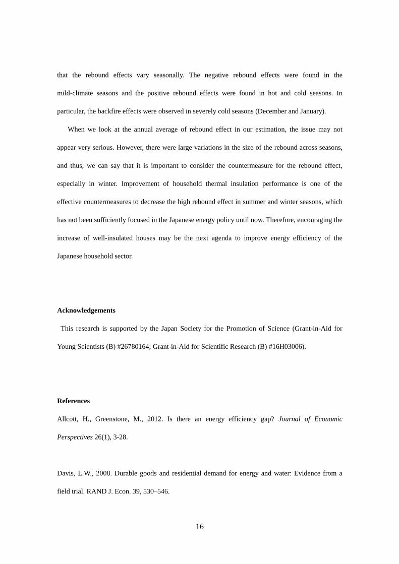
Energy efficiency of home appliances has improved considerably in the past few decades. For

example, there is a significant improvement (44.1%) in the energy efficiency of air-conditioners in

Japan between 1995 and 2015, as Figure 1 shows. Even though the change in the last decade was

modest (9.2% between 2005 and 2015), the technology is improving steadily towards lower

consumption of electricity.

// Figure 1 //

When households replace their electric appliances with new ones, one might expect power savings

as a result. Based on this expectation, policymakers often encourage the replacement of household

electric appliances with more energy-efficient ones by using policy instruments such as a subsidy

program. However, scholars have asserted that replacement to energy-efficient equipment may

induce additional energy consumption by the rebound effect: the gap between the expected saving

effect from the technological improvement and the actual saving after the energy-efficient

investment (Sorrell and Dimitropoulos, 2008). Allcott and Greenstone (2012) emphasized that the

results of many engineering or observable analyses of energy-efficient investment had been plagued

with this well-known bias.

Some studies examined the existence of the rebound effect based on the household energy

consumption (Dubin et al., 1986; Metcalf and Hassett, 1999; Davis, 2008; Davis et al., 2014). For

example, Dubin et al. (1986) analyzed the effect of an improvement in insulation on electricity

conservation by using data from 504 households in Florida. They found that the actual conservation

by insulation is 13% lower than engineering estimates for cooling and 8–12% lower for heating.

Metcalf and Hassett (1999) also analyzed the effect of improvement in insulation based on the

3

monthly electricity consumption data of the Residential Energy Conservation Survey. They also

pointed out the large gap between the estimated saving effect and the prediction based on

technological progress. Davis (2008) investigated the change in energy consumption of households

who received energy-efficient washing machines based on a field experiment. He compared the daily

power consumption of each household before and after the intervention. The results show a

significant power-saving effect after the households received a new washing machine. Moreover, the

estimated rebound effect of introducing an energy-efficient washing machine was negligible, since

the price elasticity was small. Davis et al. (2014) evaluated the effect of a large-scale program for

electric appliance replacement in Mexico, using data on 1.9 million households. They found that

replacement of refrigerators reduced electricity consumption by 8%, although this reduction was

only one-quarter of what they had expected ex ante. On the other hand, they found that households

that had replaced air-conditioners increased electricity consumption.

The methodology of the above-mentioned studies is based on the randomized control trial

(hereafter, RCT). However, social psychologists have pointed out that the RCT methodology can be

misleading, because it might invoke the Hawthorne effect. In particular, under the RCT, people

participating experiment may be conscious of being observed and this could affect their behavior.

For example, in an RCT for evaluating a given educational program, the stakeholders, namely the

school management representatives, teaching staff, parents, or guardians of the children, etc., will

visit the classroom under the experiment. The presence of these visitors may make the students of

the class conscious and thus motivate them to increase their efforts to study than usual. In this case, a

significant effect of the educational program may be erroneously found due to the Hawthorne effect,

even if there is no direct effect by the program.

This study examines the existence of the causality effect of power saving by replacement to

energy-efficient air-conditioners. We compare the monthly electricity consumption between two

4

household groups: the one that replaced their air-conditioners in the previous two years and the other

that did not do so. Since the allocation between the treatment group and the control group is not

random in our study, several socio-economic characteristics may affect the replacement behavior.

Thus, we employ the propensity score matching method to adjust the covariates (i.e., socioeconomic

characteristics) of treatment and control groups. Moreover, to control the effects of unobservable

factors, we combine the difference-in-differences method with the propensity score matching and

estimate the causality effect more rigorously.

This paper is organized as follows. Section 2 explains analytical methods of the propensity score

matching and the difference-in-differences method. In Section 3, the data used in empirical analysis

is described. Our study is based on a web-based questionnaire survey for Japanese households who

live in Kansai area. We use their monthly electricity consumption data for two years. Section 4

presents the results of our empirical analysis and discusses them. Section 5 is conclusion.

2. Empirical Methodology

This paper investigates the power-saving effect by replacing an air-conditioner with an

energy-efficient one. Here, a binary treatment indicator Di,t equals 1 if household i replaced the

air-conditioner with the energy-efficient one at time t and 0 otherwise. Letting Yi,t+1 (Di,t) be the

amount of electricity usage of household i at time t+1, the treatment effect of household i may then

be written as

)0()1(1,1,

titii

YY

Here, for each i, Yi,t+1(1) and Yi,t+1(0) are counterfactual, and only either of them is observable

(fundamental problem of causal inference). To resolve this problem, an average treatment effect on

the treated (hereafter, ATT) uses aggregate-level information, instead of individual behavioral data.

5

The ATT with regard to power-saving effect of replacing air-conditioners can be expressed as

]1/)0([]1/)1([]1/[ ,1,,1,, tititititiiATT DYEDYEDE . (1)

Here, if the assignment of the replacement of air-conditioners was random, we can replace the

second term of equation (1) ]1/)0([ ,1, titi DYE with ]0/)0([ ,1, titi DYE . That is, the mean

power consumption of households who did not replace would serve as the counterfactual outcome of

replacement households. In this case, the average treatment effect ATT would be identified.

However, if the assignment was not random, the estimates of ATT may suffer from a selection

bias. That is, observable and unobservable household characteristics, which affect the decision to

replace air-conditioners, also affect the electricity demand.

In the case of non-random assignment, the identification of ATT relies on two standard

assumptions. First is the conditional independence assumption (hereafter, CIA), which means that

conditional on the set of relevant covariates, the assignment of the treatment is independent of the

potential outcome.1 Second is the assumption of the common support. This assumption means that

households with the same covariates have a positive probability of being both treated and untreated.

In other words, each household has a positive probability of being in the treatment (replacement)

group and the control (non-replacement) group.

To establish a methodology that satisfies the above requirement for identification of ATT ,

Rosenbaum and Rubin (1983) proposed the propensity score matching methods (Heckman et al.,

1997, 1998b) and Heckman et al. (1998a) further developed this methodology. It employs a

household from the control group who has similar covariates with the household of the replacement

1 That is, although the assignment of treatment might be dependent on the observable covariates, if we control for

these covariates, we can think that the treatment was assigned almost randomly.

6

group as the counterfactual. The difference between the power consumption of the household in the

replacement group and that in the control group may then be attributed to the replacement of

air-conditioners. That is, matching mimics “randomization” by balancing the distributions of the

relevant covariates in the replacement group and the control group. Rosenbaum and Rubin (1983)

defined the probability of the treatment indicator variable that is conditional on the observable

covariates )( ii XDP as the propensity score. By matching each household between replacement

and control group based on the propensity score, we can maintain independence between the

decision of replacement (assignment) and the decision of power saving (potential outcome). The

ATT is estimated by calculating the difference of the power consumption between matched treatment

and control groups as follows:

)]/(,0/)0([)]/(,1/)1([{ ,,,1,,,,1, titititititititiCP

PSM

ATT XDPDYEXDPDYEE . (2)

Here, CP indicates the common support, which means an overlapping interval between the

propensity scores of replacement households and those of control group households.

Moreover, in a panel data setting, Heckman et al. (1997, 1998b) proposed combining the

propensity score matching with the difference-in-differences method (hereafter, DD). Their

DD-PSM estimator is defined as follows:

)]}/(,0/)0([)]/(,1/)1([{ ,,,1,,,,1, titititititititiCP XDPDYEXDPDYEEPSMDD

(3)

where 1,1,1, tititi YYY is the change in power consumption before and after the replacement.

The DD-PSM estimator can exclude the time-independent fixed effect. Heckman et al. (1997,

1998b) and Smith and Todd (2005) showed that the performance of the DD-PSM estimator is better

than that of the PSM estimator without the DD.

7

3. Data

By using an online survey, we asked households who live in Kansai area, which is comprised of

Osaka, Kyoto, Hyogo, Nara, Shiga, and Wakayama prefectures, on their status of electricity usage.2

Since the Japanese electricity retail market for households was not deregulated until April 2016,

most households in Kansai area purchased electricity from the Kansai Electric Power Co., Inc.

(KEPCO) in February and April 2015, when our survey was implemented. KEPCO provides their

customers online accessible data on their monthly electricity consumption for the past two-year

period. We requested the households to download and submit this data to us.3 We collected 733

households’ monthly electricity consumption and their responses to the survey questionnaire. Table 1

summarizes the descriptive statistics of the data.

// Table 1 //

This study regards households who switched to energy-efficient air-conditioners as the treatment

group and households who did not do so as the control group. Variables from April to January in

Table 1 are indicators of the treatment.4 The treatment is defined in terms of replacement status of

air-conditioners for the same month between 2013 and 2014. For example, April variable takes the

value of one if a household replace its air conditioner between May 2013 and March 2014.5 Thus,

2 The data collection was conducted by an online survey company. This company has their own registered

households and asked those who are living in Kansai area to participate to the survey. The participating households

are selected by first come first served basis, until the number reaches 800. 3 This data is provided in Microsoft Excel file format and includes not only the monthly electricity consumption but

also the date of meter reading, number of days of utilization, and the monthly electricity bill. 4 Since electricity consumption data is available only for two years and our survey has been implemented for two

months, data for February and March is available only for limited samples. Thus, we omitted these two months. 5 For example, a household who replaced air-conditioner in July 2013 is in the treatment group for April, May, and

June. The household is not in the treatment group for the months after July, since it uses new air-conditioner after July

2013.

8

the household recognized as the treatment by this variable uses old air conditioner in April 2013 and

new air conditioner in April 2014. Here, we also need to consider other factors than replacement that

might affect the household’s electricity consumption. For example, socio-economic variables such as

household income, number of household members, ownership and size of the house, and ownership

of the electric appliances. Temperature might be the most important factor that influences the usage

of the air-conditioners. Figure 2 shows monthly average outdoor temperature in FY2013 and

FY2014.6 There are considerable variations across months; the average temperature in the summer

of FY2013 is slightly higher than that of FY2014.

// Figure 2 //

Figure 3 and Figure 4 show the average electricity consumption (kWh/day) for each fiscal year

(FY2013 and FY2014) and each month (from April to January). The monthly electricity

consumption data provided by KEPCO does not include the amount of electricity consumption

generated by the home photovoltaic system. Thus, electricity consumption of households who have

photovoltaic system is underestimated in this data. Therefore, we exclude the households who install

the photovoltaic system with their houses from our dataset in Figure 3 and Figure 4, and also from

the analysis hereafter. For the treatment households, the FY2013 data is before the replacement and

the FY2014 data is after the replacement. Therefore, we can compare the monthly household

electricity consumption between two time points. There are two important findings from Figure 3

and Figure 4. First, power consumptions of treatment households are larger than those of control

group’s households in all months. This suggests that household characteristics significantly differ

6 The daily outdoor temperature data of many location of Japan is available from the Japan Meteorological Agency

(http://www.jma.go.jp/jma/indexe.html). Average temperature of nearest observatory is calculated based on

information of participants’ address and their days of electricity consumption for each month.

9

between the two groups. Second, the differences of power consumptions between the treatment and

control groups are smaller in FY2014 than that in FY2013. By testing the differences between two

years, we can confirm that the differences are statistically significant for April, July, August, and

September in 2013. On the other hand, the difference is statistically significant only for August in

2014. Although this might result from the replacement of the energy-efficient air-conditioners, more

rigorous statistical methodology is needed to investigate the causality effect.

// Figure 3 //

// Figure 4 //

4. Estimation results

4.1. Propensity score estimator

We begin by estimating the propensity score by using the probit model. We use a dummy variable

that takes one if the households replace the air conditioner and zero otherwise as the dependent

variable. The independent variables are variables related to home appliances (number of

air-conditioners, number of TV sets, number of refrigerators, frequency of dishwasher use, frequency

of cloth washer use, and frequency of electric kettle use), household characteristics (age of the

respondent, number of family members, number of children in elementary school age, number of

household member whose age is 65 and over, household income, marital status, whether they are

dual income family, home ownership, and whether they live in detached houses), and outdoor

temperature in 2013. Here, the outdoor temperature differs across months, and thus, we estimate the

propensity score month by month. Based on the monthly estimated propensity score, we conducted

three types of matching methods: NN matching, radius matching, and kernel matching. Generally,

10

there is a trade-off between bias and variance in each matching method. That is, if we reduce the

variance, the bias of estimate would increase (and vice versa). In the NN matching, the household in

the control group who has the value of propensity score nearest to that of the household in the

treatment group is selected as the partner of matching. However, in this method, if the value of the

propensity score of the control group household is far from that of the treatment group household,

the quality of matching decreases. To avoid this, the radius matching sets an upper limit on the value

of propensity score and targets all control households whose propensity scores fall within the certain

range. Kernel matching uses the kernel function and constructs the counterfactual dependent variable.

As this method targets almost all control group households, the size of variance is smaller than either

of the other two matching methods (in compensation, kernel matching results in the largest bias).

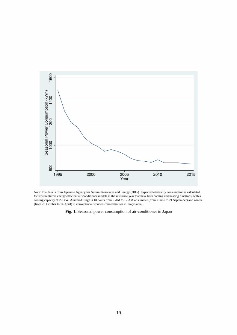
Table 2 shows the estimation results of the probit model for August 2013 and 2014.7 Before the

matching, there are many variables that have statistically significant coefficients: the numbers of

air-conditioners, TVs, and refrigerators; the frequency of using the washing machine; age;

singlehood; home ownership; size of the house; and detached house. On the other hand, no

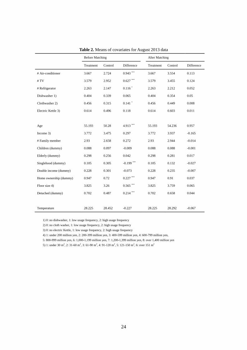
covariates have significant effect for the replacement after the matching. When we look at the result

of balance check of covariates, the sizes of mean bias are significantly diminished (Table 3). For

example, the size of mean bias of kernel matching for August is decreased from 29.9% to 4.8% by

the matching.

// Table 2 //

// Table 3 //

7 After matching, there are no statistical differences in the independent variables between the treatment and the

control groups in other months. Full estimation results are available upon requests.

11

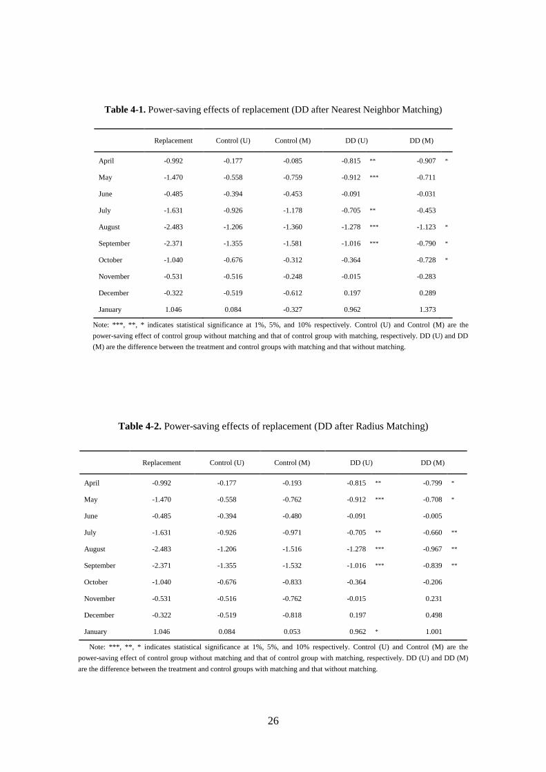
4.2. Estimation results by DD with matching

Table 4-1, 4-2, and 4-3 show the estimated power-saving effect based on the DD-PSM estimator

before and after propensity score matching for each matching method. The DD-PSM estimators

represent the difference in the change of average household electricity consumption (kWh/day) from

2013 to 2014 between treatment group and control group. Before matching, the estimators are

negative and statistically significant for April, May, July, August, and September. This result is

consistent with our expectation, since the household who replaced its air-conditioner with an

energy-efficient one can decrease its power consumption compared to the households who did not do

so. However, as we have seen in Table 2, some covariates had significant difference between

replacement and control group before matching, and these might affect the differences in electricity

consumption. To exclude the effect of these covariates, we conduct the propensity score matching.

The DD-PSM estimators after matching are shown in the right-hand side of Table 4. For NN

matching (Table 4-1), the DD-PSM estimators of April, August, September and October are negative

and significant. DD-PSM estimators of April, May, July, August and September are negative and

significant for radius and kernel matching methods. These results suggest that power-saving effects

of replacement in these months are statistically significant even after matching. Moreover, in most

cases, the sizes of DD-PSM estimators after matching are smaller than those before matching. This

means that the observable covariates have an effect on the results, and in such cases, the DD-PSM

estimator without matching would not adequately capture the treatment effect. From these estimation

results, we can confirm that the replacement of air-conditioners to energy-efficient ones would

contribute to the decrease of household power consumption especially in spring and summer

seasons.

// Table 4 //

12

4.3. The rebound effect

The analysis in subsection 4.2 suggests that the replacement of air-conditioners can decrease the

power consumption in spring and summer seasons. However, the power saving might be smaller

than the technologically expected level because of the influence of the rebound effect. On a monthly

average, our respondents had used their air-conditioners from 11.77 to 13.16 years. By using these

figures and the data on average electricity consumption by air-conditioners (Japanese Agency for

Natural Resources and Energy, 2015), we calculate the technological power-saving rate by replacing

the old air-conditioner with the new one.8 From this figure and the estimated ATT, we can calculate

the size of the rebound effect caused by replacing the air-conditioner.

Table 5 shows the sizes of the monthly estimated rebound effect. The values in the first column

are the estimated amount of electricity consumption from the air-conditioner usage by the

replacement household. Assuming that most households do not use air-conditioners in June, these

values are calculated by taking the difference between electricity consumption (kWh/day) in June

2013 and other months. There is great variability between seasons. The power consumption from

air-conditioner usage is large in August (6.50 kWh/day) and January (7.71 kWh/day), while these

values become small in the mild-climate seasons, such as October (1.88 kWh/day) and November

(1.11 kWh/day).

The monthly calculated size of the rebound effect is shown from the second to fourth columns in

Table 5. The rebound effect is calculated as follows:

8 The technological saving rate varies depending on the old air-conditioner and the new one that replaces it.

Therefore, we asked replacement households about the years in usage of their respective previous air-conditioners.

From this information, we identified the respective years of manufacture Based on the average power consumption

values of the air-conditioners that were manufactured in a given year, we estimated the power consumptions of the

previous air-conditioners. We also estimated the power consumptions of new air-conditioners by using the average

amount of power consumption of the air-conditioners that were manufactured in each year from the time of

replacement. From this information, we calculated the technological saving rate for each household that replaced its

air-conditioner.

13

(𝑅𝑒𝑏𝑜𝑢𝑛𝑑 𝐸𝑓𝑓𝑒𝑐𝑡) = {1 −(𝐴𝑐𝑡𝑢𝑎𝑙 𝑠𝑎𝑣𝑖𝑛𝑔 𝑟𝑎𝑡𝑒)

(𝑇𝑒𝑐ℎ𝑛𝑜𝑙𝑜𝑔𝑖𝑐𝑎𝑙 𝑠𝑎𝑣𝑖𝑛𝑔 𝑟𝑎𝑡𝑒)} × 100,

where the actual saving rate is calculated from the PSM-DD estimator (see Table 4) and the value of

electricity consumption of column 1 of Table 5, and the technological saving rate is calculated based

on the above method (see footnote 8).

Our results suggest that there are large variations in the rebound effect between seasons. The

rebound effect becomes positive in August, October, November, December, and January. On the

other hand, the rebound effect becomes negative in April, May, July, and September.

The negative rebound means that the electricity consumption is reduced more than

technologically expected. The result might be explained by the following reasons, the first of which

is climate. The seasons in which we found the negative rebound effect are of relatively mild climate,

such as April, May, July, and September. April and May are the spring season, and the outdoor

temperature of July and September is lower than that of August. Therefore, households might find it

easier to adopt electricity-saving measures. As Dubin et al. (1986) pointed out, the price elasticities

of the demand of cooling and heating vary according to the seasons.

The second reason is the additional function of new energy-efficient air-conditioners.

Manufacturers have introduced an additional function in recent models of air conditioners to

decrease their electricity consumption. For example, the auto power-saving mode can cut down

excess energy use automatically when the sensor perceives that there are no people in the room.

Moreover, the auto turnoff option stops the operation of air-conditioners automatically if the time of

power-saving operation continues for a given length of time. Furthermore, the auto-clean function

can clean dust on the filter automatically and makes energy-efficient operation possible. Since the

potential effect of these functions is not fully reflected in our calculation of technologically expected

14

electricity consumption, it is possible that the actual saving rate is greater than the technological

saving rate.

The third is the possibility of behavioral change of users by the provision of energy-saving

advices. Most remote control devices for the recent models of air-conditioners in Japan have a

function that shows the power-saving advices depend on the usage condition of the air-conditioner.

For example, if the room is receiving strong sunshine when an air-conditioner is working, the

message of recommendation to close a curtain is shown on the screen of remote control device.

Moreover, the amount of power consumption and estimated electricity bill based on the current

usage is indicated on the screen of remote control device and it may make the user aware of the

energy cost and encourage electricity-saving behavior. This information provision might lead to the

power-saving effect more than the theoretically expected levels.

// Table 5 //

On the other hand, we can consider two reasons for the positive rebound effect. The first is the

economic incentive. The replacement of air-conditioners might reduce the price of energy service

and lead to the increase in demand for this service (e.g., longer usage time, lower preset temperature

in summer, or higher preset temperature in winter). These additional demands may cancel out the

amount of power saving that was expected based on the technological progress (Sorrell and

Dimitropoulos, 2008). Again, the second reason is the climate. Dubin et al. (1986) showed that the

price elasticity of energy demand in winter is larger than that of summer. This means that the

rebound effect can be larger in winter. The results of our study also show that the size of the rebound

effect is large in winter season. Moreover, in winter season, the power consumption after the

replacement increases beyond the level before the replacement. This phenomenon is called the

15

“backfire effect.”

In summary, the results of our study suggest that the size of the rebound effect varies by the

season. We found that the weighted average of the rebound effect from April to January ranges from

45.1% to 58.5%. Based on the review of previous studies, Sorrell et al. (2009) summarized that the

size of the rebound effect of households in OECD countries was less than 30%. Therefore, the size

of rebound effect estimated in our study is larger than that in the previous studies.9

5. Conclusion

This study examined the causality effect from the replacement with energy-efficient

air-conditioners to decrease power consumption by comparing the replacement and non-replacement

household groups. Based on a questionnaire survey and monthly electricity consumption data in

2013 and 2014 of 733 participant households who live in Kansai area, we estimated the ATT of the

replacing air conditioners. We assumed the replacement households who replaced their

air-conditioners with the energy-efficient ones for the previous two years as the treatment group, and

the non-replacement households as the control group. From our empirical analyses, we confirmed

the significant ATT effect of the replacement, especially in summer and winter. We also showed that

the ATT with only the DD method would overestimate the ATT estimator. Moreover, ATT with only

the matching method might result in a biased ATT estimator because of the low robustness against

the unobservable factors. We estimated the rebound effect of replacing air-conditioners based on

both estimated ATT and the technological saving rate. The annual rebound effect estimated ranges

from 45.1% to 58.5%, which is slightly larger than the results of previous studies. We also confirmed

9 The rebound effect of our study targeted only the air-conditioner, while the target of Sorrell and Dimitropoulos

(2009) was households’ whole energy consumption. The difference of the size might come from this reason.

16

that the rebound effects vary seasonally. The negative rebound effects were found in the

mild-climate seasons and the positive rebound effects were found in hot and cold seasons. In

particular, the backfire effects were observed in severely cold seasons (December and January).

When we look at the annual average of rebound effect in our estimation, the issue may not

appear very serious. However, there were large variations in the size of the rebound across seasons,

and thus, we can say that it is important to consider the countermeasure for the rebound effect,

especially in winter. Improvement of household thermal insulation performance is one of the

effective countermeasures to decrease the high rebound effect in summer and winter seasons, which

has not been sufficiently focused in the Japanese energy policy until now. Therefore, encouraging the

increase of well-insulated houses may be the next agenda to improve energy efficiency of the

Japanese household sector.

Acknowledgements

This research is supported by the Japan Society for the Promotion of Science (Grant-in-Aid for

Young Scientists (B) #26780164; Grant-in-Aid for Scientific Research (B) #16H03006).

References

Allcott, H., Greenstone, M., 2012. Is there an energy efficiency gap? Journal of Economic

Perspectives 26(1), 3-28.

Davis, L.W., 2008. Durable goods and residential demand for energy and water: Evidence from a

field trial. RAND J. Econ. 39, 530–546.

17

Davis, L.W., Fuchs, A. Gertler, P., 2014. Cash for coolers: Evaluating a large-scale appliance

replacement program in Mexico. Am. Econ. J.-Econ. Polic. 6, 207–238.

Dubin, J.A., Miedema, A.K., Chandran, R.V., 1986. Price effects of energy-efficient technologies: A

study of residential demand for heating and cooling. RAND J. Econ. 17, 310–325.

EDMC. 2015. Handbook of Energy & Economic Statistics. The Institute of Energy Economics,

Quantitative Analysis Unit, Tokyo, Japan (in Japanese)

Heckman, J.J., Ichimura, H., Todd, P., 1997. Matching as an Econometric Evaluation Estimator:

Evidence from Evaluating a Job Training Program. Rev. Econ. Stud. 64, 605-654.

Heckman, J.J., Ichimura, H., Smith, J.A., Todd, P., 1998a. Characterizing Selection Bias Using

Experimental Data. Econometrica, 66, 1017-1098.

Heckman, J.J., Ichimura, H., Petra, T., 1998b. Matching as an Econometric Evaluation Estimator.

Rev. Econ. Stud. 65, 261-294.

Institute of Energy Economics, Japan. 2011. Introduction of reading way of energy and economic

data. Energy Conservation Center, Japan (in Japanese).

Japanese Agency for Natural Resources and Energy. 2015. Catalog of energy saving performance in

winter (in Japanese)

18

Joskow, P.L., Marron, D.B., 1992. What does a negawatt really cost? Evidence from utility

conservation programs. Energ. J. 13, 41–74.

Metcalf, G., Hasset, K. 1999. Measuring the energy savings from home improvement investments:

Evidence from monthly billing data. Rev. Econ. Stat. 81, 516–528.

Nishio, K., Ofuji, K., 2014. Ex-post analysis of electricity saving measures in the residential sector

in the summer of 2013. Research Report by the Central Research Institute of Electric Power Industry.

http://criepi.denken.or.jp/jp/kenkikaku/report/download/Hg1fH8WnHWLwtyvsL5Zr27KSkq1fp3Ea/

report.pdf (in Japanese).

Rosenbaum, P. R., Rubin, D.B., 1983. The Central Role of the Propensity Score in Observational

Studies for Causal Effects. Biometrika 70, 41–55.

Smith, J.A., Todd, P., 2005. Does Matching Overcome LaLonde’s Critique of Nonexperimental

Estimators? Journal of Econometrics, 125, 305-353.

Sorrell, S., Dimitropoulos, J., 2008. The rebound effect: Microeconomic definitions, limitations and

extensions. Ecol. Econ. 65, 636–649.

Sorrell, S., Dimitropoulos, J. and Sommerville, M. 2009. Empirical estimates of the direct rebound

effect: A review, Energy Policy, 37, 1356-1371

19

Note: The data is from Japanese Agency for Natural Resources and Energy (2015). Expected electricity consumption is calculated

for representative energy-efficient air-conditioner models in the reference year that have both cooling and heating functions, with a

cooling capacity of 2.8 kW. Assumed usage is 18 hours from 6 AM to 12 AM of summer (from 2 June to 21 September) and winter

(from 28 October to 14 April) in conventional wooden-framed houses in Tokyo area.

Fig. 1. Seasonal power consumption of air-conditioner in Japan

20

Fig. 2. Monthly Average Temperatures

21

Fig. 3. Average Power Consumption in FY2013

22

Fig. 4. Average Power Consumption in FY2014

23

Table 1. Descriptive statistics

Variable Obs. Mean Std.Dev Min Max

Treatment dummy

April 733 0.082 0.274 0 1

May 733 0.076 0.266 0 1

June 733 0.083 0.276 0 1

July 733 0.09 0.286 0 1

August 733 0.087 0.282 0 1

September 733 0.083 0.276 0 1

October 733 0.08 0.272 0 1

November 733 0.075 0.264 0 1

December 733 0.074 0.261 0 1

January 733 0.078 0.268 0 1

# Air-conditioner 733 2.894 1.737 0 9

# TV 733 3.022 1.195 1 8

# Refrigerator 733 2.171 0.47 1 5

Dishwasher 1) 733 0.375 0.653 0 2

Cloth washer 2) 733 0.345 0.605 0 2

Electric Kettle 3) 733 0.500 0.734 0 2

Age 733 50.327 10.559 20 69

Income 4) 733 3.557 1.741 1 8

# Family member 733 2.724 1.382 1 9

Children (dummy) 733 0.108 0.31 0 1

Elderly (dummy) 733 0.263 0.441 0 1

Singlehood (dummy) 733 0.28 0.449 0 1

Double income (dummy) 733 0.307 0.462 0 1

Home ownership (dummy) 733 0.75 0.433 0 1

Floor size 5) 733 3.375 1.372 1 6

Detached (dummy) 733 0.546 0.498 0 1

PV (dummy) 733 0.1 0.3 0 1

1) 0: no dishwasher, 1: low usage frequency, 2: high usage frequency

2) 0: no cloth washer, 1: low usage frequency, 2: high usage frequency

3) 0: no electric Kettle, 1: low usage frequency, 2: high usage frequency

4) 1: under 200 million yen, 2: 200-399 million yen, 3: 400-599 million yen, 4: 600-799 million yen,

5: 800-999 million yen, 6: 1,000-1,199 million yen, 7: 1,200-1,399 million yen, 8: over 1,400 million yen

5) 1: under 30 m2, 2: 31-60 m

2, 3: 61-90 m

2, 4: 91-120 m

2, 5: 121-150 m

2, 6: over 151 m

2

24

Table 2. Means of covariates for August 2013 data

Before Matching After Matching

Treatment Control Difference Treatment Control Difference

# Air-conditioner 3.667 2.724 0.943 *** 3.667 3.554 0.113

# TV 3.579 2.952 0.627 *** 3.579 3.455 0.124

# Refrigerator 2.263 2.147 0.116 * 2.263 2.212 0.052

Dishwasher 1) 0.404 0.339 0.065 0.404 0.354 0.05

Clothwasher 2) 0.456 0.315 0.141 * 0.456 0.449 0.008

Electric Kettle 3) 0.614 0.496 0.118 0.614 0.603 0.011

Age 55.193 50.28 4.913 *** 55.193 54.236 0.957

Income 3) 3.772 3.475 0.297 3.772 3.937 -0.165

# Family member 2.93 2.658 0.272 2.93 2.944 -0.014

Children (dummy) 0.088 0.097 -0.009 0.088 0.088 -0.001

Elderly (dummy) 0.298 0.256 0.042 0.298 0.281 0.017

Singlehood (dummy) 0.105 0.305 -0.199 *** 0.105 0.132 -0.027

Double income (dummy) 0.228 0.301 -0.073 0.228 0.235 -0.007

Home ownership (dummy) 0.947 0.72 0.227 *** 0.947 0.91 0.037

Floor size 4) 3.825 3.26 0.565 *** 3.825 3.759 0.065

Detached (dummy) 0.702 0.487 0.214 *** 0.702 0.658 0.044

Temperature 28.225 28.452 -0.227 28.225 28.292 -0.067

1) 0: no dishwasher, 1: low usage frequency, 2: high usage frequency

2) 0: no cloth washer, 1: low usage frequency, 2: high usage frequency

3) 0: no electric Kettle, 1: low usage frequency, 2: high usage frequency

4) 1: under 200 million yen, 2: 200-399 million yen, 3: 400-599 million yen, 4: 600-799 million yen,

5: 800-999 million yen, 6: 1,000-1,199 million yen, 7: 1,200-1,399 million yen, 8: over 1,400 million yen

5) 1: under 30 m2, 2: 31-60 m

2, 3: 61-90 m

2, 4: 91-120 m

2, 5: 121-150 m

2, 6: over 151 m

2

25

Table 3. Mean biases of covariates before and after matching (%)

Before matching NN matching Radius matching Kernel matching

April 31.0 9.9 5.1 4.7

May 26.7 9.7 3.3 3.2

June 27.5 9.5 3.2 3.1

July 27.5 11.1 5.4 5.0

August 29.9 11.1 5.3 4.8

September 29.9 5.4 4.9 4.7

October 28.5 10.9 4.7 4.3

November 26.4 12.9 5.1 4.6

December 24.8 11.7 5.2 4.7

January 22.1 11.9 6.9 5.3

26

Table 4-1. Power-saving effects of replacement (DD after Nearest Neighbor Matching)

Replacement Control (U) Control (M) DD (U) DD (M)

April -0.992 -0.177 -0.085 -0.815 ** -0.907 *

May -1.470 -0.558 -0.759 -0.912 *** -0.711

June -0.485 -0.394 -0.453 -0.091 -0.031

July -1.631 -0.926 -1.178 -0.705 ** -0.453

August -2.483 -1.206 -1.360 -1.278 *** -1.123 *

September -2.371 -1.355 -1.581 -1.016 *** -0.790 *

October -1.040 -0.676 -0.312 -0.364 -0.728 *

November -0.531 -0.516 -0.248 -0.015 -0.283

December -0.322 -0.519 -0.612 0.197 0.289

January 1.046 0.084 -0.327 0.962 1.373

Note: ***, **, * indicates statistical significance at 1%, 5%, and 10% respectively. Control (U) and Control (M) are the

power-saving effect of control group without matching and that of control group with matching, respectively. DD (U) and DD

(M) are the difference between the treatment and control groups with matching and that without matching.

Table 4-2. Power-saving effects of replacement (DD after Radius Matching)

Replacement Control (U) Control (M) DD (U) DD (M)

April -0.992 -0.177 -0.193 -0.815 ** -0.799 *

May -1.470 -0.558 -0.762 -0.912 *** -0.708 *

June -0.485 -0.394 -0.480 -0.091 -0.005

July -1.631 -0.926 -0.971 -0.705 ** -0.660 **

August -2.483 -1.206 -1.516 -1.278 *** -0.967 **

September -2.371 -1.355 -1.532 -1.016 *** -0.839 **

October -1.040 -0.676 -0.833 -0.364 -0.206

November -0.531 -0.516 -0.762 -0.015 0.231

December -0.322 -0.519 -0.818 0.197 0.498

January 1.046 0.084 0.053 0.962 * 1.001

Note: ***, **, * indicates statistical significance at 1%, 5%, and 10% respectively. Control (U) and Control (M) are the

power-saving effect of control group without matching and that of control group with matching, respectively. DD (U) and DD (M)

are the difference between the treatment and control groups with matching and that without matching.

27

Table 4-3. Power-saving effects of replacement (DD after Kernel Matching)

Replacement Control (U) Control (M) DD (U) DD (M)

April -0.992 -0.177 -0.206 -0.815 ** -0.786 *

May -1.470 -0.558 -0.768 -0.912 *** -0.702 *

June -0.485 -0.394 -0.470 -0.091 -0.014

July -1.631 -0.926 -0.991 -0.705 ** -0.640 **

August -2.483 -1.206 -1.533 -1.278 *** -0.951 **

September -2.371 -1.355 -1.526 -1.016 *** -0.845 **

October -1.040 -0.676 -0.843 -0.364 -0.197

November -0.531 -0.516 -0.784 -0.015 0.253

December -0.322 -0.519 -0.808 0.197 0.487

January 1.046 0.084 0.102 0.962 * 0.952

Note: ***, **, * indicates statistical significance at the 1%, 5%, and 10%, respectively. Control (U) and Control (M) are the

power-saving effects of control group without matching and that of control group with matching, respectively. DD (U) and DD (M)

are the differences between the treatment and control groups with matching and that without matching.

28

Table 5. Rebound effects of replacement of energy efficient air-conditioner

Month

Electricity use by

air-conditioner in

2013 (kWh/day)

Rebound effect (%)

NN Radius Kernel

April 4.04 -32.33 -16.58 -14.80

May 2.52 -70.72 -70.01 -68.45

June - - - -

July 1.61 -57.33 -129.22 -122.30

August 6.50 8.38 21.08 22.44

September 4.24 2.92 -3.10 -3.84

October 1.88 -93.68 45.06 47.69

November 1.11 -28.61 204.91 215.16

December 4.45 133.64 157.85 156.64

January 7.71 192.47 167.43 164.09

Annual

(April-January) 45.13 58.08 58.46